Embed Size (px)
Citation preview

POUR L'OBTENTION DU GRADE DE DOCTEUR ÈS SCIENCES
PAR
Maîtrise de physique, Université Paris VI, France
acceptée sur proposition du jury:
Prof. O. Martin, pésident du juryProf. B. Deveaud-Plédran, directeur de thèse
Prof. H. Brune, rapporteur Dr Le Si Dang, rapporteur Prof. J. Tignon, rapporteur
0D MICROCAVITY POLARITONS TRAPPING LIGHT-MATTER QUASIPARTICLES
Ounsi EL DAÏF
THÈSE NO 3815 (2007)
ÉCOLE POLYTECHNIQUE FÉDÉRALE DE LAUSANNE
PRÉSENTÉE LE 6 JUILLET 2007
À LA FACULTÉ DES SCIENCES DE BASE
Laboratoire d'optoélectronique quantique
SECTION DE PHYSIQUE
Suisse2007

2

Contents
Abstract/resume/moulakhas . . . . . . . . . . . . . . . . . . . . . 8
Introduction 15
I A new kind of structure 19
1 Framework 211.1 Elements of optical properties of semiconductors . . . . . . . 21
1.1.1 Band structure and excitons . . . . . . . . . . . . . . . 211.1.2 Excitons confined in a quantum well . . . . . . . . . . 23
1.2 Cavities: light confinement . . . . . . . . . . . . . . . . . . . 241.2.1 Bragg mirrors . . . . . . . . . . . . . . . . . . . . . . . 241.2.2 Microcavity . . . . . . . . . . . . . . . . . . . . . . . . 25
1.3 Strong coupling . . . . . . . . . . . . . . . . . . . . . . . . . . 271.3.1 Principles . . . . . . . . . . . . . . . . . . . . . . . . . 271.3.2 Lifetimes and spectral broadening . . . . . . . . . . . 291.3.3 Polariton nonlinearities . . . . . . . . . . . . . . . . . 301.3.4 Experimental signatures of strong-coupling . . . . . . 301.3.5 The strong to weak coupling transition . . . . . . . . . 32
1.4 The bosonic character of polaritons . . . . . . . . . . . . . . . 331.4.1 Validity of the bosonic nature of excitons . . . . . . . 331.4.2 Bose-Einstein condensation of polaritons . . . . . . . . 34
1.5 Confinement of 2D polaritons . . . . . . . . . . . . . . . . . . 351.5.1 Why? . . . . . . . . . . . . . . . . . . . . . . . . . . . 351.5.2 A state of the art of polariton confinement . . . . . . 351.5.3 And now... how? . . . . . . . . . . . . . . . . . . . . . 361.5.4 Orders of magnitude . . . . . . . . . . . . . . . . . . . 371.5.5 . . . . . . . . . . . . . . . . . . . . . . . . . . . . . . 39
2 Conception and fabrication of the sample 412.1 Preliminary . . . . . . . . . . . . . . . . . . . . . . . . . . . . 41
2.1.1 General idea . . . . . . . . . . . . . . . . . . . . . . . 412.1.2 Materials used . . . . . . . . . . . . . . . . . . . . . . 42
3

4 CONTENTS
2.1.3 Characteristics of local growth methods . . . . . . . . 432.1.4 The structure chosen . . . . . . . . . . . . . . . . . . . 442.1.5 Mesas . . . . . . . . . . . . . . . . . . . . . . . . . . . 452.1.6 In situ cleaning and regrowth . . . . . . . . . . . . . . 472.1.7 Simulation . . . . . . . . . . . . . . . . . . . . . . . . 47
2.2 Growth of a microcavity with embedded mesas . . . . . . . . 472.2.1 First growth and characterization . . . . . . . . . . . . 482.2.2 Photolithography . . . . . . . . . . . . . . . . . . . . . 502.2.3 Chemical etching . . . . . . . . . . . . . . . . . . . . . 522.2.4 Final sample . . . . . . . . . . . . . . . . . . . . . . . 54
2.3 Conclusion and improvement of the method . . . . . . . . . . 562.3.1 Step by step improvement . . . . . . . . . . . . . . . . 562.3.2 Conclusion: a satisfactory sample . . . . . . . . . . . . 57
II Physical studies 59
3 Zero and two dimensional strong-coupling regimes 613.1 Experimental considerations . . . . . . . . . . . . . . . . . . . 613.2 Characterization of the 2D cavities . . . . . . . . . . . . . . . 633.3 Strong-coupling regime in zero dimension . . . . . . . . . . . 66
3.3.1 Strong-coupling in small mesas . . . . . . . . . . . . . 663.3.2 The doublet: a lift of degeneracy . . . . . . . . . . . . 693.3.3 Larger mesas . . . . . . . . . . . . . . . . . . . . . . . 703.3.4 Comment on the linewidths and high Q-factors . . . . 71
3.4 Conclusion: a high quality confinement of strongly coupledquasiparticles . . . . . . . . . . . . . . . . . . . . . . . . . . . 72
4 Spectroscopy of polaritons in the real and reciprocal spaces 734.1 Spectroscopy . . . . . . . . . . . . . . . . . . . . . . . . . . . 73
4.1.1 Experimental setup . . . . . . . . . . . . . . . . . . . . 734.1.2 Reciprocal space spectroscopy . . . . . . . . . . . . . . 744.1.3 Real space spectroscopy . . . . . . . . . . . . . . . . . 784.1.4 Relaxation processes . . . . . . . . . . . . . . . . . . . 794.1.5 Theoretical description of confined polaritons . . . . . 804.1.6 Conclusion . . . . . . . . . . . . . . . . . . . . . . . . 83
4.2 2D images through resonant excitation . . . . . . . . . . . . . 844.2.1 Set-up . . . . . . . . . . . . . . . . . . . . . . . . . . . 844.2.2 Resonant Rayleigh scattering in 2D . . . . . . . . . . 854.2.3 Images of a 9 micron mesa . . . . . . . . . . . . . . . 864.2.4 Images of a 19 micron mesa . . . . . . . . . . . . . . . 884.2.5 Images of a 3 micron mesa . . . . . . . . . . . . . . . 904.2.6 Interpretation . . . . . . . . . . . . . . . . . . . . . . . 914.2.7 Conclusion . . . . . . . . . . . . . . . . . . . . . . . . 93

CONTENTS 5
5 Studies in the nonlinear regime 955.1 Motivation and general phenomenology of power studies . . . 95
5.1.1 General case . . . . . . . . . . . . . . . . . . . . . . . 955.1.2 Case of polaritons . . . . . . . . . . . . . . . . . . . . 96
5.2 Non-resonant excitation . . . . . . . . . . . . . . . . . . . . . 995.2.1 Regimes observed . . . . . . . . . . . . . . . . . . . . . 995.2.2 Weak coupling regime . . . . . . . . . . . . . . . . . . 1045.2.3 A lab for seeing nonlinear effects . . . . . . . . . . . . 107
5.3 Resonant excitation: parametric processes . . . . . . . . . . . 1095.3.1 Principles of parametric processes . . . . . . . . . . . 1095.3.2 Setup . . . . . . . . . . . . . . . . . . . . . . . . . . . 1105.3.3 Parametric processes in the 2D cavity . . . . . . . . . 1115.3.4 Parametric processes in a 9µm mesa . . . . . . . . . . 1145.3.5 Continuous wave pumping of a 9µm mesa . . . . . . . 1165.3.6 Resonant excitation of a 3µm mesa at zero detuning . 1185.3.7 Alternative points of view: signs of bistability? . . . . 120
5.4 Balance and conclusions . . . . . . . . . . . . . . . . . . . . . 1235.4.1 Balance of the observed phenomena . . . . . . . . . . 1235.4.2 Conclusion . . . . . . . . . . . . . . . . . . . . . . . . 124
III Perspectives and discussions 127
6 Applications 1296.1 Polariton single photon source . . . . . . . . . . . . . . . . . . 129
6.1.1 Principle . . . . . . . . . . . . . . . . . . . . . . . . . 1306.1.2 Potential advantages . . . . . . . . . . . . . . . . . . . 131
6.2 Twin photon source in the near infrared . . . . . . . . . . . . 1316.2.1 Existing devices and principle . . . . . . . . . . . . . . 1316.2.2 Feasibility with 0D polaritons: use of polariton para-
metric scattering . . . . . . . . . . . . . . . . . . . . . 1316.2.3 Advantages of 0D polaritons . . . . . . . . . . . . . . 132
6.3 Feasibility . . . . . . . . . . . . . . . . . . . . . . . . . . . . . 1336.3.1 Global warming! . . . . . . . . . . . . . . . . . . . . . 134
7 Experimental perspectives 1357.1 Perspectives on this sample . . . . . . . . . . . . . . . . . . . 135
7.1.1 Time-resolved studies . . . . . . . . . . . . . . . . . . 1367.1.2 Complete imaging of the confined modes . . . . . . . . 1377.1.3 Further nonlinear studies . . . . . . . . . . . . . . . . 137
7.2 The next generation of samples . . . . . . . . . . . . . . . . . 1377.2.1 A new sample structure . . . . . . . . . . . . . . . . . 1387.2.2 Improving fabrication methods . . . . . . . . . . . . . 139

6 CONTENTS
7.3 New trap shapes: from simple confinement to condensate in-terference . . . . . . . . . . . . . . . . . . . . . . . . . . . . . 1397.3.1 A new mask . . . . . . . . . . . . . . . . . . . . . . . . 1397.3.2 Multiple etchings: stairway to... ? . . . . . . . . . . . 1417.3.3 Electron-beam lithography . . . . . . . . . . . . . . . 141
7.4 And now... just do it? . . . . . . . . . . . . . . . . . . . . . . 142
8 Conclusion 143
Epilogue: Between applied and basic research 147
IV Appendices 151
A Theoretical description 153
B Clean room/Salle blanche 157B.1 Parameters used for photolithography . . . . . . . . . . . . . 157B.2 Recapitulatif des points critiques en salle blanche . . . . . . . 158B.3 Diffraction limit in the case of photolithography . . . . . . . . 159
C Various works 161C.1 Diploma works on 0D polaritons . . . . . . . . . . . . . . . . 161C.2 Quantum well and microcavity samples characterization . . . 162
Bibliography 162
CV 175
Acknowledgments/Reconnaissance 178

7

8 CONTENTS
Abstract
Polaritons are half-matter half-light quasiparticles, arising, in a two-dimensional semiconductor microcavity, from the strong-coupling betweenan exciton (an elementary electronic excitation of a crystal) and a photon.This thesis presents the fabrication of polariton confining structures, theircharacterization and the study of the linear and non-linear optical propertiesof the confined polaritons.
Thanks to their bosonic character, to their extremely light effective massand to the peculiar shape of their dispersion curve, polaritons were provento accumulate in their ground state to form a Bose-Einstein condensate ina CdTe based sample, at a high temperature of the order of 20 Kelvin.No such effect was observed in GaAs materials, who offer a less disorderedenvironment, where we developed a method to fabricate traps of any shapeand size. The latter should facilitate the condensation of polaritons bylowering the density thresholds, and allow us to manipulate the condensate.
Thanks to the strong-coupling regime, it is possible to confine polaritonseither through their photon or through their exciton part. We thus fab-ricated two-dimensional microcavities with local thickness variations, con-fining the cavity photon along its two free dimensions. We were able toperform this through high-quality molecular beam epitaxy (MBE) growth,accompanied by a controlled processing of the sample. We measured theanticrossing behaviors characteristic of the strong-coupling regime in zeroand two dimensions. As the confining structures have sizes of the order ofthe micron, we could image the confined polaritons’ wave functions in thereal and reciprocal (momentum) spaces, and tried to understand how thetransition between confined (0D) and extended (2D) polariton modes oc-curs. We also gave first evidences of the interaction between the two andzero-dimensional structures, and of the polariton trapping from one to theother.
We then studied the nonlinear optical properties of this new object,performing two different kinds of experiments:
1. a study of the response of the system to a non-resonant excitation, inorder to probe the formation of a condensed phase. Collective elec-tronic excitations were created, at energies far higher than the modeswhich are of interest for us. We observed the effect of high densitiesin the system and evidenced Coulomb interaction. We then observedthe cross-over from strong to weak-coupling regime, and the onset oflasing in the weakly coupled system.
2. a study of the response of the system to a resonant excitation in orderto probe parametric effects between the discrete states. In this con-

CONTENTS 9
figuration a number of polaritons are intentionally created in a givenstate. We observed various nonlinear behaviors as a function of thecreated population, which may be interpreted as effects of Coulombinteraction, or indications of bistable behaviors in the system. Wewere nevertheless not able to discriminate.
We give some potential applications in the field of single or correlatedphoton emission. Although industrial applications may not be in the short-term agenda, it should be possible to take advantages of this original type ofstructures for research and development applications. We finally give someexperimental perspectives, which may help deepen the observations shownand the interpretations proposed here, and should allow to work towardsthe fabrication of new samples, where BEC of polaritons is observed andcontrolled, as well as parametric oscillations between various confined states.
Keywords: polaritons; strong-coupling; microcavities; semiconductor quan-tum dots; excitons; photoluminescence; nonlinear optics; semiconductorlasers.

10 CONTENTS
Resume
Polaritons de microcavite a 0DPiegeage de quasi-particules matiere lumiere
Les polaritons sont des particules mixtes matiere lumiere, resultant, dansune microcavite semi-conductrice a deux dimensions, du couplage fort entreun exciton (l’excitation electronique elementaire d’un cristal) et un photon.Cette these presente la fabrication et la caracterisation de structures confi-nant les polaritons, ainsi que l’etude des proprietes optiques lineaires et nonlineaires des polaritons confines.
La condensation de Bose Einstein de polaritons –accumulation macro-scopique de population dans l’etat fondamental du systeme– a ete observeedans une microcavite basee sur du CdTe. Cette condensation a eu lieu a unetemperature elevee, avoisinant les 20 degres Kelvin. Elle a ete possible gracea la nature bosonique des polaritons ainsi qu’a leur petite masse effective,et enfin a la forme particuliere de leur courbe de dispersion. Les materiauxbases sur le GaAs offrent quant a eux une structure moins desordonnee,dans laquelle nous avons developpe une methode de fabrication de pieges den’importe quelle taille ou forme. Ces derniers devraient favoriser la conden-sation des polaritons (non-observees encore dans ces materiaux) en baissantles seuils en densite, et nous permettre de manipuler l’eventuel condensat.
Grace au couplage fort, il est possible de confiner les polaritons a traversl’une de leurs composantes: le photon ou l’exciton. Nous avons donc fabriquedes micro-cavites bidimensionnelles dans lesquelles nous avons localement in-troduit une legere variation d’epaisseur, permettant de confiner le photon dumode de cavite le long de ses deux dimensions libres. Nous avons realise cettestructure par epitaxie par jet moleculaire (MBE) de haute qualite, accom-pagnee d’un procede de modification de l’echantillon. Nous avons mesurela courbe d’anticroisement caracterisant le couplage fort pour les differentesstructures a zero et a deux dimensions presentes sur l’echantillon. Commeles pieges ont des tailles de l’ordre du micron, nous avons pu realiser optique-ment des images de la fonction d’onde des polaritons dans les espaces reelet reciproque (l’espace des impulsions). Nous avons essaye de comprendrecomment la transition entre un systeme a 0D et un systeme a 2D se fait.Nous avons de plus mis en evidence des interactions entre les polaritons 2Det 0D, ainsi que le mecanisme de piegeage des uns vers les autres.
Nous avons ensuite etudie les proprietes optiques non lineaires de cenouvel objet, a travers deux types d’experiences :
1. une etude de la reponse du systeme a une excitation non resonante,pour permettre l’eventuelle formation d’une phase condensee. Nousavons cree des excitations electroniques en grand nombre a des energiestres elevees par rapport aux energies des modes qui nous interessent.

CONTENTS 11
Nous avons pu observer des effets dus aux hautes densites atteintesdans le systeme, nous avons observe l’effet des interactions coulombi-ennes. Nous avons enfin observe le passage du couplage fort vers lecouplage faible, et le demarrage des oscillations laser (de type VCSEL)dans le systeme en couplage faible.
2. une etude de la reponse du systeme a une excitation resonante, poursonder les effets parametriques entre les etats discrets. Dans cette sit-uation des polaritons sont crees intentionnellement dans un etat. Nousavons observe plusieurs comportements non lineaires de l’emission enfonction de la population creee, qui peuvent etre interpretes commedes effets des interactions coulombiennes, ou comme des signes de com-portement bistable du systeme, sans reussir a distinguer l’interpretationla plus pertinente.
Nous avons propose des applications potentielles, basees sur la struc-ture developpee dans ce travail, pour l’emission de photons uniques oucorreles. Meme si ces applications ne sont pas encore realistes en termesindustriels, il serait possible d’utiliser ce type de structures pour la rechercheappliquee. Nous proposons enfin des perspectives experimentales qui pour-raient aider a approfondir nos observations et les interpretations que nousen avons proposees, et devraient permettre d’avancer dans la fabrication denouveaux echantillons, dans lesquels la condensation de Bose-Einstein despolaritons pourra etre observee et maıtrisee, et dans lesquels des oscillationsparametriques entre des modes confines pourraient avoir lieu.
Mots-cles : polaritons; couplage fort; microcavites; boıtes quantiques semi-conductrices; excitons; photoluminescence; optique non lineaire; lasers asemiconducteurs.

12 CONTENTS
من حالة ثنائية البعد إلى احلالة امللتقطة.
فيما بعد فقد قمنا بدراسة اخلواص الضوئية الالخطية لذلك املركب اجلديد بناء على نوعني مختلفني منالتجارب:- دراسة ملدى إستجابة النظام لإلثارة الالجتاوبية و ذلك بهدف سبر تشكل الطور املتكاثف. شكلنا١
إثارة إلكترونية متجمعة عند طاقات عالية جدا و هي غير متوافقة مع الطاقات التي تهمنا. بناء على هذهالتجربة فلقد الحظنا تأثير الكثافات العالية في اجلملة و الذب يثبت التفاعل املتبادل الكولومبي. منثم الحظنا إنتقال اجلملة من حالة الترابط القوي إلى حالة الترابط الضعيف من جهة و بروزها كمادة فعالة
لليزر في حالة الترابط الضعيف من جهة أخرى.- دراسة ملدى إستجابة اجلملة لإلثارة التجاوبية و ذلك لسبر األحداث البارامترية بني السويات املنفصلة٢
بفضل اإللتقاط. تنشأ حتريضيا في هذه احلالة اإلختبارية عدد من البوالريتونات في سوية معينة.الحظنا عدد من التصرفات الالخطية كتابع لإلسكان املتكون للبوالريتونات، و ميكن إن يعود هذا األمرإما إلى التأثير الكولومبي املتبادل أو إلى ثنائية احلالة في اجلملة (حالتي الترابط القوي و الضعيف). و
حتى اآلن ال ميكن التمييز بني احلالتني.
مت برهان و وصف اخلواص و الظواهر املرافقة إضافة إلى إعطاء بعض التطبيقات: فالتطبيقات الصناعية منهاليست في القريب املنظور، أما التطبيقات املحتملة فتتضمن إصدار الفوتونات األحادية و املترابطة التي ميكنإستخدامها في البحث العلمي و التطبيقي. خالصة لهذا البحث فقد قدمنا بعض املنظورات التي ممكن أن تقودإلى فهم أعمق للمالحظات التي بنيناها سابقا و لإلشارات و التفسيرات التي اقترحناها في هذا البحث. هذهالنتائج ستفتح هجال عمل هيتقبلي متعلق بتحضير عينات جديدة يظهر فيها تكاثف بوز- أينشتاين و
اإلهتزاز البارامتري بني سويات ملتقطة.
: بوالريتونات، ترابط قوي، فجوة ميكروية، أنصاف نواقل دو البعد صفر، أكسيتون،الكلمات األساسيةاصدار، البصريات الالخطية، لبزرات أنصاف النواقل.

CONTENTS 13
ملخصبوالريتونات فجوية ذو بعد صفر
إلتقاط شبه جزيئات أنصاف مادة و أنصاف ضوء
البوالريتونات هي أشباه جزيئات و توصف بأنها ذات طبيعة مزدوجة (أنصاف مادة و أنصاف ضوء) و هي تظهرمن الترابط القوي بني األكسيتون (ثنائية إلكترون ثقب) و الفوتون و ذلك في فجوة ميكروية ثنائية األبعاد و منأنصاف النواقل. هذا البحث هبني على دراستي. األولى تقدم إنتاج بنية محددة للبوالريتونات باإلضافة إلى
دراسة خواصها. أما الثانية فدراسة للخواص اخلطية والالخطية للبوالريتونات.
إن التوصيف البوزوني و الكتلة الفعالة اخلفيفة باإلضافة إلى الشكل املميز لتابع التشتت في هذا النوع من املوادبرهت على أنها العامل في التراكم في السوية األساسية. و هذا التي تشكل تكاثف بوز- أينشتاين في عينات
كلفن).٢٠ عند درجات احلرارة العالية (CdTeالكادميوم - تلوريوم
(التي لم تشهد ذلك التكاثف) مواد ذات ترتيب أكبر في محيطها. و بناءGaAsتقدم مادة الغاليوم - زرنيخ على هذا األمر فقد قمنا بتطوير طريقة جديدة لتصنيع لواقط أبرزت فعاليتها مهما شكلها أو قياسها. هذهاللواقط ينبغي أن تسهل تكاثف البوالريتونات عبر تخفيض كثافة حاجز العتبة سامحة لنا التحكم بهذا
التكاثف.
إن منطقة الترابط القوى متكن حصر البوالريتونات في جزئيها الفوتوني أو األكسيتوني. إللتقاط الفوتونالفجوي ضمن مساره ذو البعد الثنائي، قمنا بتصنيع فجوة ميكروية ثنائية األبعاد و ذات سماكة متغيرة ببعض
) وMBEاملواقع املحددة. إستطعنا تشكيل هذه الفجوة ذات اجلودة العالية عبر منو للبورات حسب طريقة ال(ذلك بترافق مع القدرة على التحكم بهندسة العينة املصنعة. إضافة إلى ذلك فقد قمنا بدراسة خواص الالتصالبفي الفضاء احلقيقي كما في فضاء اإلندفاع و هما مييزان منطقة الترابط القوي في العينة و ذلك في احلالتني: حالة
ثناائية البعد و حالة البعد صفر ، في اللواقط.
إن الكتلة الفعالة اخلفيفة للبوالريتونات تكفي إلعطاء البنية املحددة أبعادا مساوية للميكرومتر. األمر الذيمنحنا إمكانية تصوير التوابع املوجية للبوالريتونات املحصورة، و ذلك ضمن الفضائني احلقيقي و اإلندفاعي. وقد إقترحنا أيضا كيفية حدوث اإلنتقال من ثنائية األبعاد إلى البعد صفر. في نفس اإلطار و ألول مرة متكنا منتقدمي برهان يدل على التفاعل املتبادل بني اجلزيئات الثنائية األبعاد و ذوات البعد الصفر، إذ إن فعل اإللتقاط يتم

14 CONTENTS

Introduction
Most of the major advances in semiconductor physics and technology overthe last thirty years originated from quantum confinement of elementaryexcitations along one, two, or three spatial dimensions [Hess et al., 1994,Bimberg et al., 1999] and from the improvement of their coupling to theelectromagnetic field. Indeed confinement in semiconductor structures al-lows the study of various fundamental effects, ranging from the Purcell effect[Purcell, 1946] to full quantum confinement. Such confinement is also usedfor applications in many fields, ranging from optoelectronics to quantuminformation.
The various studies carried out in the past decades were focused on onehand on matter, through the confinement of excitonic resonance in quan-tum wells, quantum wires and quantum dots, and on the other hand onthe electromagnetic field’s environment, modified by optical confinement indifferent types of cavities. Additionally, since the mid-nineties, low dimen-sional devices have been designed in the strong coupling regime, yieldingthe observation of polaritons –eigenstates of semiconductor microcavities instrong coupling regime [Weisbuch et al., 1992]. Confinement can enhanceinteractions, and can modify the real and imaginary parts of the resonances’energies, or can allow new interaction processes.
In this context, quantum dots represent the model system since theyallow quasi-zero-dimensional confinement of electronic states and display adiscrete spectrum of energy levels. Quantum dots are usually generated bya process of spontaneous formation, resulting in a broad distribution of sizesand shapes [Bimberg et al., 1999]. This in turn limits the control over theenergy-level structure and makes single-dot applications a challenging task.In this framework, 0D strong-coupling involving single or a very few numberof particles is of high interest for the study of cavity quantum electrodynamiceffects in semiconductors.
Research on solid state systems has also been motivated, during the last50 years, by the ability to achieve Bose-Einstein condensation (BEC) at hightemperature. This effect involves a huge number of particles, that massivelyaccumulate into a single quantum state below a critical temperature, thusdisplaying macroscopic quantum properties. Bose-Einstein condensation ofmicrocavity polaritons was recently demonstrated in a CdTe based microcav-
15

16 CONTENTS
ity [Kasprzak et al., 2006]. These quasi-particles have the great advantageover excitons or electrons to exhibit a very light effective mass. BEC wasfavored by a confinement of the polaritons within small volumes [Kasprzaket al., 2006] in local defects of the microcavity (unintended in this case) anaspect confirmed by theoretical works (see in particular [Sarchi and Savona,2006]).
0D Polaritons confinement can be achieved either through their excitonicor photonic component. Recently, evidence for 0D polaritons has been givenwith single quantum dots in micropillars [Reithmaier et al., 2004], photonicnanocavities [Yoshie et al., 2004, Hennessy et al., 2007], or microdisks [Peteret al., 2005] and for a large number of excitations in micropillar structures[Bloch et al., 1998, Obert et al., 2004, Dasbach et al., 2001]. Here we considera novel system under the strong coupling regime, where 0D confinement isachieved through the photonic part of polaritons in high Q cavities. Ouroriginal structure contains mesas in the spacer layer of a semiconductormicrocavity, allowing confinement of the cavity photon whilst keeping thestrong coupling regime, creating thus confined polaritons. We performedspatial and spectral mapping of the polariton modes that allowed us todirectly observe their squared wave function. We also performed studiesunder the nonlinear regime, exciting, through their photon component, ahigh number of polaritons interacting through their excitonic component.
We will first present a general outline of this work and then pass ratherrapidly from the general to the direct context of polariton confinement. Wewill see at the end of chapter 1 how we decided to proceed in order to confinepolaritons.
In chapter 2 we will see this choice of procedure is not straightforward,and we will elaborate on the tools necessary to conceive and build high-quality microcavity structures with patterned mesas. We will follow thewhole process of the fabrication of the sample on which we focused in thiswork.
We will then characterize the structure we were able to build. In chapter3 we will ensure that the strong-coupling regime is present in the sample.Then in chapter 4, we will perform a spectroscopic study of the wave func-tions of the polaritons (resulting from the strong-coupling) in the real andreciprocal (momentum) spaces. We will see that this can also be done sur-prisingly efficiently without spectroscopic means.
After characterizing the sample, we will study its nonlinear properties.Chapter 5 consists of two different parts: the first one shows the response ofthe system to a non-resonant excitation, where collective electronic excita-tions were created at energies far higher than the modes which are of interestto us. The second part of the chapter shows the response of the system to aresonant excitation, where a number of polaritons are intentionally created

CONTENTS 17
in a desired state.We will present some potential applications in chapter 6, and some ex-
perimental perspectives on the sample studied herein or on new samples, inchapter 7.
We will then conclude in chapter 8, and, as concluding does not meanending, we will add some remarks on this research in an epilogue, not to beconsidered as part of this thesis work.
Finally, the last part (numbered part IV) of this manuscript will consistof several appendices. The first one deals with the theoretical description ofour system, The others will not necessarily be of high interest to the reader,but will be of high interest to my friends and successors, since they includemany useful details about the various tests and parameters used during thebuilding and characterization processes.

18 CONTENTS

Part I
A new kind of structure
19


Chapter 1
Framework
We will give, in this first chapter, some important tools necessary to under-stand the experiments presented in this work1. We will also make a briefoverview of the state of the art in strongly coupled semiconductor micro-cavities.
In the last part (1.5) of the chapter, we will more specifically introducethe context of this work, which aim is to confine polaritons along the threedimensions of space. We will develop what has been done by various groups,and we will discuss some preliminary issues, necessary to start the followingchapter about the conception and fabrication of the sample.
1.1 Elements of optical properties of semiconduc-tors
1.1.1 Band structure and excitons
The state of an atom is usually given by its electronic configuration. In acrystal, a macroscopic number of atoms is periodically stacked. In an idealcase, the eigenstates of such a system are given by the electronic configu-rations of the crystal. These electronic states are characterized by a bandstructure in the (E,~k) space, were E is the bands energy and ~k the wave vec-tor of the electrons. Between the various bands, some energy ranges (gaps)are forbidden to the electrons.
In most semiconductors, the valence band is completely filled with elec-trons and split in several subbands with different angular momentum. Whenthe maxima of the conduction and valence band are at the same k-vector,one speaks of a direct gap, when they show different k-vectors, one speaks
1Section 1.1 to 1.4 of this introductory chapter are based on the theoretical descrip-tion of polaritons performed by Vincenzo Savona [Savona et al., 1999], on the thesis ofJean-Philippe Karr [Karr, 2001], Stefan Kundermann [Kundermann, 2006], and MaximeRichard [Richard, 2004].
21

22 CHAPTER 1. FRAMEWORK
-10
-8
-6
-4
-2
0
2
E(k
)
-4 -2 0 2 4
k
Valence Band (J=1/2)
Valence Band (J=3/2)
Conduction Band (J=3/2)
gap
Figure 1.1: Band structure of a III-V semiconductor with a direct gap.
of an indirect gap. Without any excitation the valence band is filled withelectrons and the conduction band empty. When one simply mentions thegap, it is a reference to the energy gap between these two bands.
The dispersion curves E(k) can be approximated by parabola aroundk = 0, one can then identify the corresponding electrons to free particlesand associate to each curve an effective mass m∗ defined in the followingway:
E(k) = E(k = 0) +~2k2
2m∗ (1.1)
When an electron is excited from the valence band to the conductionband, it leaves behind a vacancy which is called a hole. Electrons andholes occupying the conduction or valence bands are attributed effectivemass m∗corresponding to the curvature of their dispersion curve. They arecalled, as a function of their spin, heavy holes (spin ±3/2) or light holes spin(±1/2).
Excitons
The optical properties of the crystal depend on the energy of the gap, Egap.The crystal can be optically excited by an electromagnetic wave, it willabsorb photons with energies higher than Egap. In this process a photonexcites an electron which passes from the valence band to the conductionband. A electron-hole pair is then created.
But the absorption spectrum of a semiconductor crystal shows also asharp peak at energies lower than the gap. This peak is due to the creationof an electron-hole pair bound by Coulomb interaction, called the exciton.The energy of this excitonic resonance is then given by:
EX(K) = Egap − Eb +~2K2
2mX(1.2)

1.1. ELEMENTS OF OPTICAL PROPERTIES OF SEMICONDUCTORS23
Where Eb is the binding energy of the exciton, ~K is its momentum andmX its effective mass, given by 1
mX= 1
m∗e
+ 1m∗
h. As there are two types of
holes, there are two types of excitons: the heavy and the light exciton, withdifferent energies2 and masses.
The exciton system is similar in a way to the hydrogen atom. Thehamiltonian is identical and the various exciton levels can also be labeled1s, 2s, 2p etc.
1.1.2 Excitons confined in a quantum well
By stacking semiconductor materials with different gap energies one canconfine excitons along one, two or three dimensions of space, creating quan-tum wells (planar structures), quantum wires (1D structure), or quantumdots (0D structures, sometimes referred as quantum boxes). As we workedon 2D structures, we will focus on the confinement of excitons along onespatial dimension, thus confinement towards two dimensions.
A quantum well is a 2D layer of a given semiconductor material stackedbetween two semiconductor materials with larger bandgaps, as shown onFig.1.2, thus creating an energy well. The confinement energy of the excitonsis, in a first approximation, given by the following expression of a particlein a 1D potential well with infinite barriers:
Econf =~2π2
2m∗L2(1.3)
where L is the width of the quantum well along the confinement direc-tion, we will choose this direction as the z direction of a usual cartesianframe.
z growth axis
E (eV)Gap energy
In0.05
Ga0.95
As
GaAs
GaAs
1.351 1.425
L
Figure 1.2: Energy profile of an InGaAs in GaAs Quantum Well at roomtemperature, from [Nahory et al., 1978] cited in [Palmer, 2001].
As the mass of the various heavy and light excitons (and the excitonswith various angular momentum) vary, the quantum well shows an energysplitting between these exciton.
2Although energies are often degenerate at k = 0, in particular in bulk GaAs.

24 CHAPTER 1. FRAMEWORK
One can apply this description to the material used in this study. As wewill see, our sample includes a quantum well consisting of an Indium gal-lium arsenide with 5% of indium (In0.05Ga0.95As) layer of L = 8nm width,stacked between bulk Gallium Arsenide (GaAs), whose band structure showsa higher energy gap than the one of InGaAs, see Fig.1.2.
1.2 Cavities: light confinement
The second element of the system we intend to study is an optical micro-cavity. The microcavity is a Fabry-Perot cavity entirely fabricated in solidstate, including the spacer between the two mirrors. The mirrors are dis-tributed Bragg reflectors (or Bragg mirrors), they have several importantadvantages: a very high reflectivity (on a certain range of wavelengths), thefact that they can be grown as the quantum well and in the same molecularbeam epitaxy (MBE) chamber, and the fact that, as they are interferentialmirrors, they do not heat under high powers as metallic mirrors. The cavityis designed in order to show a resonance at the energy of the quantum wellexciton energy.
1.2.1 Bragg mirrors
Bragg mirrors can be seen as a one-dimensional photonic crystal. Photoniccrystals are structures with a periodic refractive index, and this periodicity,as in the case of electronic crystals (the semiconductor we saw above), yieldsthe appearance of photonic gaps usually called stopband. The index period-icity can be compared to the potential periodicity in electronic crystals. Thecalculation which shows the appearance of this gap is really similar to theone performed in a usual crystal, and yields the appearance of energy gaps,using the Bloch theorem. The book of Joannopoulos [J.D.Joannopouloset al., 1995] shows clearly the analogy and the calculations.
In order to obtain the index periodic structure, pairs of layers of twodifferent natures are stacked. In our case they consist of ≈ 40 alternativelayers of AlAs and GaAs (so 20 pairs), having a refractive index of 3.526and 2.926 at ≈ 10K and at a wavelength around 835nm, as calculated withequations given in ref. [Adachi, 1990], the stopband is proportional to theindices’ ratio and has here a width of around 100nm in wavelength. Thecentral wavelength λ0 of the stopband is related to the optical thickness ofthe mirrors through the relation: λ0/4 = niei, with i = GaAs or AlAs, andei the physical thickness of each layer.
In order to probe this photonic gap and the photonic modes allowed inBragg mirror, one can simply perform a reflectivity experiment. Indeed thephotonic gap yields a very high reflectivity. One can see an example of thisstopband calculated through transfer matrix based simulations on Fig.1.3,the values taken correspond to the values we will concretely use later: 22.5

1.2. CAVITIES: LIGHT CONFINEMENT 25
0 500 1000 1500 2000 2500 30001
1.5
2
2.5
3
3.5
4
position (nm)
Re
fra
ctio
n in
de
x
Dielectric structure: light incident from left side (air)
1.25 1.3 1.35 1.4 1.45 1.5 1.55 1.6 1.65 1.70
0.2
0.4
0.6
0.8
1
Energy (eV)
Re
fle
ctivity
Figure 1.3: Upper figure: refractive index profile. The starting layer on theleft is air, and the last layer on the right is the substrate. Lower figure:Reflectivity spectrum.
pairs of 59.4 nm GaAs and 71.6 nm AlAs. We will focus further on thesecalculations in the next chapter.
1.2.2 Microcavity
Two Bragg mirrors are stacked to form an optical cavity around a GaAs layerof thickness l, called the cavity spacer. As the spacer index is lower thanthe index of the first mirror layer (AlAs), the cavity modes at the interfacebetween the cavity spacer and the first mirror layer show an antinode. Theresonance wavelengths of such a cavity are given by nGaAsl = lopt = N λN
2with N a positive integer and lopt the effective optical thickness of the cavity.
We chose to study what we will from now on call a λ-cavity, because wewill focus on the N = 2 cavity mode, which is given by lopt = λ2 = λ. Thismode is chosen to be resonant with the exciton’s wavelength: λN=2 = λX =λ.
The Bragg mirrors are designed in such a way that this same λ is thecentral wavelength of their stopband. λ is a resonance wavelength of thecavity and the electromagnetic field is thus admitted inside the cavity withthis wavelength. The reflectivity spectrum shows thus a dip, as one cansee on Fig.1.4. Again this reflectivity spectrum was simulated using theparameters of the sample which we will study in this work, as we will se inthe next chapter.

26 CHAPTER 1. FRAMEWORK
0 1000 2000 3000 4000 5000 60001
1.5
2
2.5
3
3.5
4
position (nm)R
efr
actio
n in
de
x
Dielectric structure: light incident from left side (air)
1.3 1.35 1.4 1.45 1.5 1.55 1.6 1.65 1.70
0.2
0.4
0.6
0.8
1
Energy (eV)
Re
fle
ctivity
Figure 1.4: Refractive index profile (upper figure) and reflectivity spectrum(lower figure) of a λ-cavity.
Dispersion of the cavity photon
There is a dependence of the cavity resonance on the angle of incidence of thefield with respect to normal incidence. The cavity imposes a quantization
Mirror
kyk
zk
Spacer
Mirror
!
kx
Figure 1.5: Sketch of the cavity, the incident wave vector and its componentson z and the plane of the cavity. θ is the angle of incidence.
of the wave vector in the growth direction, which we chose to be z, so letus write ~k in terms of its component kz along z and ~k|| = kx~x + ky~y (seeFig.1.5) in the plane parallel to the layers (x, y): ~k = ~k|| + ~kz. Thus one canwrite:
E =hc
nGaAsλ= ~ck/nGaAs = ~c(
√k2
z + k2||)/nGaAs (1.4)
one can deduce a dispersion relation
E(k||) =
√E2
z +~2c2k2
||
n2GaAs
(1.5)
This equation is parabolic-like around k|| = 0, thus one can again, as for

1.3. STRONG COUPLING 27
the exciton, attribute an effective mass to the cavity photon, deduced fromthe curvature of equation 1.5 at k|| = 0:
mphot =nGaAsh
λc(1.6)
Where λ is, as mentioned before, the cavity N = 2 resonance wavelengthat normal incidence. For a resonance wavelength of 800nm, equation 1.6yields a mass of mphot = 1.4 10−36kg. The photon dispersion curvaturearound k|| = 0 is thus 104 times bigger than the exciton’s curvature. Thisgives a mass of the order of 10−5 the free electron’s mass, or 10−4 theexciton’s mass.
Quality factor and Finesse
A cavity is an optical resonator. Resonators are characterized through twovalues measuring the time during which energy is stored compared to theloss rate. The quality factor is defined as follows: [Saleh and Teich, 1991]
Q =2π (stored energy)
energy loss per cycle=
ν0
δν(1.7)
where ν0 is the resonance considered and δν is its spectral linewidth.As one can see the quality factor depends on the considered mode (which
determines the energy stored in the resonator). The finesse is defined as afunction of the free spectral range νF and can be linked to the quality factoras follows:
F =νF
ν0Q (1.8)
The best quality factors in optical cavities can reach 108 in dielectricmicrospheres [Mie, 1908, Braginsky et al., 1989], where strong coupling witha single nanocrystal has recently been observed by LeThomas et al. [2006].
In semiconductor microcavities as presented here, the best quality factorsreach 20−30000 [Stanley et al., 1994, Daıf et al., 2006b, Sanvitto et al., 2005].
1.3 Strong coupling
1.3.1 Principles
It is known since the pioneering work of Purcell [Purcell, 1946], that a 2-levelatom placed at the antinode of a standing electromagnetic wave in a Fabry-Perot cavity, sees its emission probability enhanced. If the coupling betweenthe atom and the electromagnetic wave is sufficient, meaning that the energyexchange is faster than the coherence decay of each, the eigenmodes of thesystem are a superposition of the atomic excited state and the cavity mode(or cavity photon), this system is called the dressed atom.

28 CHAPTER 1. FRAMEWORK
The situation is similar for a quantum well embedded in a microcavity.When the coupling between the exciton and the cavity photon is sufficientlystrong, one observes new eigenmodes in the system called polaritons. Wewill rapidly see how these modes can be written.
The hamiltonian of the coupled exciton photon system reads as follows:
H0 =∑k||
Ec(k||)a†k||
ak|| +∑k||
EX(k||)b†k||
bk|| +∑k||
~ΩR(a†k||bk|| + b†k||ak||)
(1.9)where a†k|| , ak|| and b†k|| , bk|| are respectively the creation and annihilation
operators of photons and excitons with an in-plane vector ~k||, and ~ΩR isthe coupling energy. It depends on the overlap between the exciton’s andphoton’s wave functions, given by the design of the cavity.
The energies of the eigenstates of the hamiltonian 1.9 are:
E±(k||) =Ec(k||) + EX(k||)
2± 1
2
√(δk||)
2 + 4|~ΩR|2 (1.10)
whereδk|| = Ec(k||)− EX(k||) (1.11)
is the detuning between the cavity mode energy and the quantum well ex-citon energy. This quantity will often be used in the coming pages. Whensimply mentioning the detuning, we will from now on mean its value atk|| = 0: δk||=0.
In the absence of coupling (~ΩR = 0), the eigenstates of this system aresimply the uncoupled photon and exciton. Otherwise, the system is in a”strong coupling regime” and a splitting between EX(k = 0) and Ec(k = 0)occurs, the latter are not anymore the eigenstates of the system, the energiesavailable to the system are E+ and E−. The new eigenstates of the systemare the upper and lower polaritons. Fig.1.6 shows the polaritons’ dispersioncurves, compared to the uncoupled exciton and photon dispersion curves.
The polaritons’ operators are written as follows in the original photon-exciton basis: (
pk
qk
)=(
Xk Ck
−Ck Xk
)(bk
ak
)where p†k, pk and q†k, qk are the creation and annihilation operators for
the lower and upper polariton, respectively, and Xk and Ck are the Hopfieldcoefficients, introduced by Hopfield in 1958 [Hopfield, 1945-1946], they areequal to:
Xk|| =1√
1 + ( ~ΩRE−(k||)−Ec(k||)
)2, Ck|| =
1√1 + (E−(k||)−Ec(k||)
~ΩR)2
(1.12)
1.3. STRONG COUPLING 29
8
4
0
En
erg
y (
meV
)
-4 -2 0 2 4
k (1/!m)
15
10
5
0En
erg
y (
meV
)
-4 -2 0 2 4
k (1/!m)
12
8
4
0
En
erg
y (
meV
)
-4 -2 0 2 4
k (1/!m)
-2
0
2
En
erg
y (
meV
)
-4 -2 0 2 4
Detuning (meV)
EUP
ELP
Eexc
Ecav EUP
ELP
Eexc
Ecav EUP
ELP
Eexc
EcavEUP
ELP
Eexc
Ecav
EUP
ELP
Eexc
Ecav
(a)
(b) (d)(c)
12
8
4
0
En
erg
y (
meV
)
-4 -2 0 2 4
k (1/!m)
EUP
ELP
Eexc
Ecav
EUP
ELP
Eexc
EcavEUP
ELP
Eexc
Ecav
"R
"R
"R
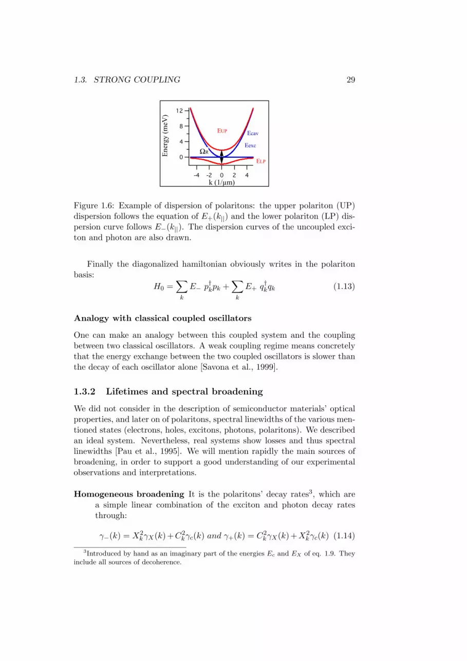
Figure 1.6: Example of dispersion of polaritons: the upper polariton (UP)dispersion follows the equation of E+(k||) and the lower polariton (LP) dis-persion curve follows E−(k||). The dispersion curves of the uncoupled exci-ton and photon are also drawn.
Finally the diagonalized hamiltonian obviously writes in the polaritonbasis:
H0 =∑
k
E− p†kpk +∑
k
E+ q†kqk (1.13)
Analogy with classical coupled oscillators
One can make an analogy between this coupled system and the couplingbetween two classical oscillators. A weak coupling regime means concretelythat the energy exchange between the two coupled oscillators is slower thanthe decay of each oscillator alone [Savona et al., 1999].
1.3.2 Lifetimes and spectral broadening
We did not consider in the description of semiconductor materials’ opticalproperties, and later on of polaritons, spectral linewidths of the various men-tioned states (electrons, holes, excitons, photons, polaritons). We describedan ideal system. Nevertheless, real systems show losses and thus spectrallinewidths [Pau et al., 1995]. We will mention rapidly the main sources ofbroadening, in order to support a good understanding of our experimentalobservations and interpretations.
Homogeneous broadening It is the polaritons’ decay rates3, which area simple linear combination of the exciton and photon decay ratesthrough:
γ−(k) = X2kγX(k)+C2
kγc(k) and γ+(k) = C2kγX(k)+X2
kγc(k) (1.14)
3Introduced by hand as an imaginary part of the energies Ec and EX of eq. 1.9. Theyinclude all sources of decoherence.

30 CHAPTER 1. FRAMEWORK
Inhomogeneous broadening It is due to both the quantum well andthe cavity disorder. The quantum well shows a static disorder [Zim-mermann, 1995, Savona, 2007] due to impurities or inhomogeneitiespresent in the growth process. The cavity mode is broadened due toroughness of the interfaces between the layers of the Bragg mirrors[Christmann et al., 2006].
1.3.3 Polariton nonlinearities
We have considered in the description of the system in section 1.3 only linear(first order) terms, this is valid at low densities, at higher densities, severalnonlinear phenomena can occur, the most relevant one in the frame of thiswork is the excitonic Coulomb interaction, which can yield the scattering oftwo excitons and can be written as follows: [Ciuti et al., 2003]
HX−X =12
∑k,k′,q
VX−Xb†k+qb†k′−qbkbk′ (1.15)
This term, if it becomes dominant, yields nonlinear effects, which we willrapidly mention here, we will come back on these effects in more detail inchapter 5 (nonlinear studies).
• Parametric luminescence [Ciuti et al., 2001], where collisions are themain population mean of given states k′ − q and k + q, its populationshows a nonlinear dependence on the initial population of states k, k′.
• Parametric oscillations, analog to the optical parametric oscillator[Savvidis et al., 2000, Stevenson et al., 2000, Ciuti et al., 2000], whichcan lead to giant parametric amplification [Saba et al., 2001] and allowcoherent control [Kundermann et al., 2003].
• A broadening of the exciton’s linewidth, yielding a broadening of thepolaritons linewidths through equation 1.14.
• A blueshift of the exciton’s resonance, and thus of the polariton res-onance, depending lineraly on the excitation intensity [Ciuti et al.,2001].
1.3.4 Experimental signatures of strong-coupling
In order to characterize experimentally the strong coupling regime, one needsto observe the splitting between the two upper and lower polaritons at res-onance between the exciton and the cavity photon. Several experiments arepossible, based on reflection or transmission of an incident electromagneticbeam, in order to probe the optical density of states, or based on photolu-minescence experiments. We will develop these methods in chapter 3.
1.3. STRONG COUPLING 31
In all the methods, spectra are taken on various positions of the cavity,and in case of strong coupling, two modes can be seen around the resonanceenergy instead of one degenerate. Nevertheless, this single observation couldbe attributed to many phenomena different than strong-coupling, as theobservation of light-hole exciton for example. The certainty of the strong-coupling regime can be brought only by an anticrossing behavior. Two kindsof behaviors can be observed (See Fig.1.7 for illustration):
8
4
0
Ener
gy (
meV
)
-4 -2 0 2 4
k (1/!m)
12
8
4
0
Ener
gy (
meV
)
-4 -2 0 2 4
k (1/!m)
12
8
4
0Ener
gy (
meV
)
-4 -2 0 2 4
k (1/!m)
-2
0
2
Ener
gy (
meV
)
-4 -2 0 2 4
Detuning (meV)
EUP
ELP
Eexc
Ecav EUP
ELP
Eexc
Ecav EUP
ELP
Eexc
EcavEUP
ELP
Eexc
Ecav
EUP
ELP
Eexc
Ecav
(a)
(b) (d)(c)
12
8
4
0Ener
gy (
meV
)
-4 -2 0 2 4
k (1/!m)
EUP
ELP
Eexc
Ecav
EUP
ELP
Eexc
EcavEUP
ELP
Eexc
Ecav
"R
"R
"R
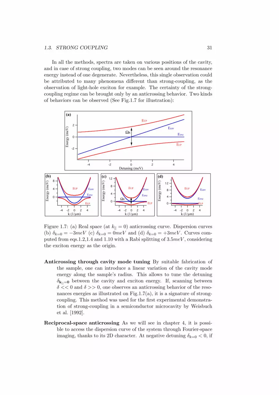
Figure 1.7: (a) Real space (at k|| = 0) anticrossing curve. Dispersion curves(b) δk=0 = −3meV (c) δk=0 = 0meV and (d) δk=0 = +3meV . Curves com-puted from eqs.1.2,1.4 and 1.10 with a Rabi splitting of 3.5meV , consideringthe exciton energy as the origin.
Anticrossing through cavity mode tuning By suitable fabrication ofthe sample, one can introduce a linear variation of the cavity modeenergy along the sample’s radius. This allows to tune the detuningδk||=0 between the cavity and exciton energy. If, scanning betweenδ << 0 and δ >> 0, one observes an anticrossing behavior of the reso-nances energies as illustrated on Fig.1.7(a), it is a signature of strong-coupling. This method was used for the first experimental demonstra-tion of strong-coupling in a semiconductor microcavity by Weisbuchet al. [1992].
Reciprocal-space anticrossing As we will see in chapter 4, it is possi-ble to access the dispersion curve of the system through Fourier-spaceimaging, thanks to its 2D character. At negative detuning δk=0 < 0, if

32 CHAPTER 1. FRAMEWORK
one observes an anticrossing behavior at a certain value of k > 0 andat the symmetrical value −k, see Fig.1.7(b), it is an anticrossing char-acteristic of strong-coupling. A non-parabolic dispersion for the lowerpolariton dispersion curve (Figs.1.7(b)-(d)) is another characteristicfeature of strong-coupling. This method was first experimentally usedfor a semiconductor microcavity in strong-coupling in 1994 by Houdreet al..
We will base our work on these two methods. We will use the first methodto demonstrate strong-coupling in our sample in chapter 3, and illus-trate it using the second method in chapter 4. Two other methods,that we will not use, are also possible:
Temperature tuning It is possible to tune the exciton’s energy throughtemperature tuning. This method is usually used when it is not possi-ble to vary the cavity mode’s energy, for the demonstration of strong-coupling of a single quantum dot with a cavity. This method was usedfor example in refs. [Peter et al., 2005, Reithmaier et al., 2004, Yoshieet al., 2004].
Time-resolved studies It is finally possible to demonstrate strong-couplingby directly observing in the time domain the energy exchange (theRabi oscillations) between the two polariton modes, this method wasfor example used in ref. [Norris et al., 1994].
1.3.5 The strong to weak coupling transition
The system shows strong-coupling for sufficient coupling strength ΩR. Whenwriting the total hamiltonian, including coupling terms4, the coupling strengthis replaced at resonance by the quantity
Ω′R =
√Ω2
R − (γc(k)− γX(k))2
which depends on the coupling strength and on the linewidths of the coupledoscillators [Savona et al., 1999]. This quantity is the vacuum Rabi splitting.It is the energy difference between the two polariton modes at resonancebetween the exciton and cavity photon.
Due to the finite lifetime5 of the cavity photon and of the exciton, a con-dition sine qua non for strong-coupling is that the energy exchange shouldbe faster than the decay rates, this can be written as follows:
ΩR > γX , γc (1.16)
4e.g. to phonons5In the exciton’s case, one should say coherence time, as it is shorter than the lifetime,
but it is the cavity photon lifetime which is the limiting parameter.

1.4. THE BOSONIC CHARACTER OF POLARITONS 33
One can now give some objective criteria for the recognition of the transi-tion6 from strong to weak coupling regimes. Starting from a strong-couplingregime situation, the strong-coupling can be lost for two reasons:
If γc and/or γX increase Concretely the most probable situation is anincrease of the exciton’s linewidth γX , due to various effects we willdescribe in section 1.4.
If ΩR decreases ΩR is the coupling strength between the excitons and the
photons. It depends on the exciton’s oscillator strength (ΩR ∝√
fS ).
The strong-coupling regime can be therefore lost by saturation of theexcitonic oscillator strength, in other terms by loss of the bosoniccharacter of excitons, and in even simpler terms, by loss of the excitonsin favor of electron-hole pairs. This happens at high densities, as shownby equation 1.18.
Experimentally, the way to interpret this is by a double inequality aderived from 1.16:
Ω′R > γ−, γ+ (1.17)
When the splitting between the polaritonic resonances is smaller than thelinewidth of each of the two modes, it is in practice nearly impossible todistinguish them anymore.
1.4 The bosonic character of polaritons
1.4.1 Validity of the bosonic nature of excitons
Excitons are bosons composed of fermions as can be an atom, with a big dif-ference regarding the binding energy. The latter is 13.6eV for the hydrogenatom and of the order of several meV for the excitons in III-V semiconduc-tors, so much lower. This means that excitons are fragile bosons!
As an exciton state is spread over a high number of electronic states ina crystal. Pauli’s exclusion principle does not forbid a big occupancy of anexciton state, as long as the system is at low density. At high densities,the occupation of the electronic states increases, Pauli’s exclusion principleapplies and makes it more and more difficult to create new excitons.
This can be summed up by writing the commutator of the exciton’screation and annihilation operators [Haug and Koch, 1990] (which shouldbe exactly equal to one for a perfect boson):
[b, b†] ∼ 1−O(na2B) (1.18)
6The use of the word transition should not lead the reader to understand phase tran-sition, as there is no order parameter build-up in this case, the transition is progressive.

34 CHAPTER 1. FRAMEWORK
where aB is the exciton’s Bohr radius. The critical density over whichthe exciton can not be considered as a boson anymore is thus ∼ 1/a2
B.In the case of an In0.05Ga0.95As in GaAs quantum well, the Bohr radiusis approximately aB ' 12nm [Grassi Alessi et al., 2000]. This yields acritical density n0 ∼ 7.1011cm−2, consistent with experimental values ofabout ∼ 1011cm−2.
This is a cause of loss of strong-coupling, as it leads to both featuresdescribed in section 1.3.5.
1.4.2 Bose-Einstein condensation of polaritons
The aim of the structure we are introducing in this work is to favor a Bose-Einstein condensation (BEC) of polaritons. Let us therefore have a shortlook at the properties of a polariton BEC phase.
Bosons can show a spectacular transition to a peculiar condensed phase:Bose-Einstein condensation. This condensation sees a macroscopic numberof bosons accumulate in the ground state of a system, a lot has been writtensince its prediction by Bose and Einstein [Bose, 1924, Einstein, 1924] till itsdiscovery in 1995 in ultracold atomic gases. In these systems temperaturesof the order of the nK need to be reached. In this sense, polaritons, as longas they can be considered as bosons (in the low density limit) are of greatinterest as they have a very small effective mass in comparison to the exciton(thanks to their photonic component), which theoretically should allow themto show a temperature of condensation higher than 0.1K [Kavokin et al.,2003].
The open character of the polariton system, due to their extremelyshort lifetime, questions however the thermodynamic equilibrium necessaryto reach condensation. It was demonstrated that despite this openness, itis possible to observe a thermodynamic equilibrium under certain densityconditions [Kasprzak et al., 2006], in the same reference, Kasprzak et al.unambiguously observe Bose-Einstein condensation. Three key points wereobserved and allowed them to infer BEC :
Accumulation of population in the ground level of the system supportedby an evaluation of its occupancy number, found to be macroscopic(>> 1).
Long-range order The mean correlation length jumped from ∼ 3µm (thede Broglie wavelength) to ∼ 13µm.
Thermodynamic equilibrium The distribution of population along stateshaving higher energies than the ground state was found to be a Boltz-mann distribution.
1.5. CONFINEMENT OF 2D POLARITONS 35
1.5 Confinement of 2D polaritons
Spatial trapping of polaritons, the main subject of this work, should favorBEC. We will now see in more detail the motivation of this trapping, andwhat is the method chosen to achieve it.
1.5.1 Why?
In order to obtain a condensed phase in semiconductors, the peculiar trapshape of the lower microcavity polariton dispersion curve has motivatedseveral relaxation experiments towards the bottom of this ”trap” [Richard,2004, Richard et al., 2005]. Nevertheless, when this work started, no polari-ton condensation was unambiguously demonstrated yet. And it appearedthat, along with the ”trapping” along the dispersion curve, spatial confine-ment of polaritons, yielding the apparition of discrete polariton states, wasneeded. Indeed confinement increases the density of polaritons per state,without increasing the global density of excitons per cm2. This should helpreaching the condensation threshold of more than one polariton per state,while avoiding the loss of the strong coupling regime and of the bosoniccharacter of polaritons.
Bose-Einstein condensation has now been observed in a cadmium tel-luride microcavity sample (II-VI semiconductor) [Kasprzak et al., 2006]. Itappears that spatial confinement on the micron scale, due to an importantphotonic disorder present in this kind of materials [Richard, 2004], alongwith the peculiar dispersion curve, was a key element that allowed conden-sation of polaritons.
Thanks to the light effective mass of polaritons, a lateral confinement onthe micron scale is sufficient to achieve quantization of the polariton states– a quite unique situation in a semiconductor artificial structure that makesfabrication, positioning and optical addressing much easier than for othernanostructured systems.
1.5.2 A state of the art of polariton confinement
Attempts to produce spatially confined polariton states, in the past, havebeen made by etching micropillars of a few µm in diameter from an initiallyplanar microcavity [Bloch et al., 1998],[Dasbach et al., 2001],[Gutbrod et al.,1998]. These structures have in general proved to be able of producinglateral confinement of polariton modes. However, they tend to display strongcoupling only in the limit of very small diameter [Bloch et al., 1998], typicallyin the 1-2 µm range. Sometimes the spectral signature of the upper polariton– needed as a proof of the formation of polaritons as normal modes of thelinear exciton-photon coupling – is absent, as in ref. [Dasbach et al., 2001].In this reference the linewidth of the confined lower polariton is rather high.

36 CHAPTER 1. FRAMEWORK
These two features are probably due to the fact that the confined mode,at such small mesa diameter sizes, are coupled to the free 3D continuumthrough the lateral walls of the pillar. Indeed the lateral wall of the mesa isdirectly in contact with air, and shows disorder, allowing the electromagneticwaves to scatter.
Gerard et al. studied the confinement energies of pillar microcavities in1996. Later on, in the same group, Lalanne et al. [2004] have studied thequality factor of pillar microcavities depending on their diameter [Lalanneet al., 2004], and have shown that a lower diameter limit exists, below whichthe Q-factor decreases very rapidly, again because of the interface roughness,that favors the coupling with the 3D continuum of electromagnetic modes.In their case it is at around 0.5µm but this limit depends on the materialand interface quality of the studied sample.
Added to the basic confinement, several nonlinear phenomena were ob-served in such pillar microcavities in strong-coupling regime. Parametricoscillations in 1D microcavities was observed in a unique kind of linear sam-ple by Dasbach et al. [2005]. Parametric oscillations and luminescence werereported in refs. [Dasbach et al., 2001, Bajoni et al., 2007].
For sake of exhaustivity, let us mention another way of confining polari-tons, through the electronic excitations’ confinement in quantum dot struc-tures, placed in micro or nanoresonators. These systems are not candidatesfor BEC, as only one polariton is created, but are of great interest for cavityquantum electrodynamics experiments. This was achieved by three groups[Peter et al., 2005, Reithmaier et al., 2004, Yoshie et al., 2004] a couple ofyears ago. The main problem of this technique is the difficulty to place eas-ily the quantum dot at an antinode of the cavity field. This was solved byBadolato et al. in 2005, who reported the observation of Purcell enhance-ment of the quantum dot emission through a suitable placement. This ledthem recently to the observation of strong-coupling regime between a singlequantum dot and a photonic crystal nanocavity [Hennessy et al., 2007].
1.5.3 And now... how?
The idea developed at the LOEQ for the lateral confinement of polaritonis inspired from the state of the art presented above, in the sense thatthe polaritons are to be confined through their photonic component. It ishowever different in the sense that the whole cavity is not etched. Theidea is simply to create locally, on the spacer layer of a usual 2D sample, athicker cavity, along several microns. This creates, locally, a slightly thickercavity, see Fig.1.8. As equation 1.4 shows, Ec(x) ∝ 1
l(x) , thus the thickercavity lowers the cavity photon energy, and finally, if the strong coupling ispreserved, the polariton energy.
We will simply call these local thickness variations mesas, these mesasact as traps for the cavity photons, and thus for the polaritons.

1.5. CONFINEMENT OF 2D POLARITONS 37
l=! l'=!'=!+"!
Mirror
Figure 1.8: Principle of cavity photon confinement: local variation of thecavity thickness.
This method shows a priori several advantages, which will mostly beconfirmed by the measurements presented in the next chapters.
Tunable trap depth The depth of the trap with respect to the surround-ing 2D cavity is tunable, as it is directly related to the physical depthof the mesa. We will see that it is sufficient to produce a mesa heightof the order of the nanometer.
No lateral losses The lateral interface is reduced to the minimum, as themesas show height of the order of the nm, and there are no accessiblestates out of the mesa at the suitable energies. Compared to themicropillar walls which height is ∝ µm, this reduces lateral losses,which are an important limitation to strong coupling [Obert et al.,2004].
Multidimensionality On the example shown on Fig.1.8, it is clear thatthe 2D and 0D structures coexist, one can thus imagine interactionbetween the corresponding polaritons. There is also in principle thepossibility of having 1D structures, coupled to neighboring structuresof any in-plane shape.
No size limitation As the surrounding environment is the 2D structure,there is no possibility of coupling with a continuum of external modes,and thus the lower size limitation shown in ref. [Lalanne et al., 2004]does not apply.
1.5.4 Orders of magnitude
In order to have a rough idea of the depth of our trap, we need to recallthe fact that we want the strong coupling regime to be present both inthe mesas and around, and we want to be near resonance, in order to beable to observe the degeneracy lifting. Which means that we would like theconfining potential V to be smaller than or of the order of the Rabi splitting

38 CHAPTER 1. FRAMEWORK
V . ΩR, 3.6meV in our case, equivalent to a cavity thickness variation of≈ 3nm.
In order to have a rough idea of the width to give to our trap, we calcu-late orders of magnitudes, simply considering the polariton as 2D particlesof mass m, confined in a cylindrical well. Leyronas and Combescot pub-lished a very useful paper [Leyronas and Combescot, 2001] giving analyticalexpressions for the bound states of quantum wells, wires and dotes. Weapplied the case of cylindrical wire confinement to our situation.
They sum up the problem through a dimensionless parameter ν definedas follows:
V =~2ν2
2mR2(1.19)
where V is the energy depth of the confining potential, m the mass of theconfined particles and R the radius of the cylinder.
To every given confinement depth V and width (radius R), one can at-tribute a ν through equation 1.19. Leyronas and Combescot give then ananalytical expression of a parameter α, which labels the confined levels,allowing to calculate their number and energies through the following equa-tion: E = ~2α2
2mR2 . As we are using this model to obtain a first idea, it isenough here to show the graphic results on figure 1.9.
!"#$% &'( )*% +#((,%( *%,-*) ,! !.!.!"." # -,/%0 +#((,%( #+%)1%%0 )1' !%2,"'034")'(! "#0 #55%#( #! *,-* '( $'13%5%03,0- '0 )*% "'060%2%0) %7)%0!,'08 )*% $#(-%( )*% "9)*% +%))%( )*% # ! ! #55('7,2#),'0 &'( )*% !#2% #: ;0 ')*%(1'(3!9 60,)% +#((,%(! %&&%")! #(% -',0- )' +% /%(< ,25'()#0)&'( !)('0-$< "'060%3 !<!)%2!: ='$$'1,0- >?: @AB9 1% #(% $%3 )' 2%#!4(% )*% 5#(),"$%
%0%(-,%! ,0 )*% !#2% 40,) #! #9 0#2%$<
$ ! !.!.!.!". ! # " !.".!.!". ".#
C')% )*#) &'( " ! D" )*% %0%(-< ,! "$'!% )' )*% )'5 '& )*%1%$$ 1*,$% &'( " ! #"! ,! "$'!% )' D !' )*#) )*% $%/%$ ,! 3%%5,0!,3% )*% 1%$$:=('2 )*% )(#0!"%03%0)#$ %?4#),'0 /%(,6%3 +< )*% /#(,'4!
%0%(-< $%/%$! '& )*%!% "'060%3 -%'2%)(,%! -,/%0 +%$'19 1%603 )*#) )*% 042+%( '& +'403 !)#)%! ,! "'0)('$$%3 +< )*%5'!,),'0 '& )*% 5#(#2%)%( # 1,)* (%!5%") )' # !%) '& /#$4%!#2,0 #) 1*,"* # +'403 !)#)% -%)! '4) '& )*% 1%$$9 ,:%: 3,!E#55%#(!: F "#(%&4$ !)43< '& )*,! )(#0!"%03%0)#$ %?4#),'0!*'1! )*#) )*% 5#(#2%)%( ! '& )*% +'403 !)#)% $%/%$! +%*#/%!#! !2#7!"A# #"A# 1*%0 # $ !" #03 #! #2,0 # $"#" #2,0#1*%0 # $ #2,0# G*% )*(%% 5#(#2%)%(! @#2,09 !2#79 $B '& )*%!%#!<25)')," +%*#/,'(! 3%5%03 '0 )*% -%'2%)(< '& )*%"'060%2%0) #03 )*% $%/%$ 403%( "'0!,3%(#),'0:
" ='( ?4#0)42 1%$$!9 )*% $%/%$! #(% "*#(#")%(,H%3 +< '0%?4#0)42 042+%( %9 1,)* % ! A" ." I"&" )*% "'((%!5'03E,0- 5#(#2%)%(! +%,0- #2,0 ! "% " A#%!." !2#7 ! %%!.#03 $ ! A#
" ='( "<$,03(,"#$ 1,(%!9 )*% $%/%$! #(% "*#(#")%(,H%3 +< )1'?4#0)42 042+%(! % #03 !! 1,)* ! ! D" A" ."&# ='( )*%@%9 !!B $%/%$!9 )*% 5#(#2%)%( ,! $ %?4#$ )' A!!45"!" A#")*% 5#(#2%)%( !2#7 ,! %?4#$ )' )*% %)* H%(' '"%#! '& )*%J%!!%$ &40"),'0 (! #03 )*% )*(%!*'$3 #2,0 &'( $%/%$
)* +,-./%012 3* 4/!5,16/7 8 9/:;< 9707, 4/!!=%;607;/%1 >>? @ABB>C DE>FDEGKI.
=,-: A: G*% %0%(-< 5#(#2%)%( ! #! 3%60%3 ,0 >?: @.B &'( )*% %)*+'403 !)#)%! '& # ?4#0)42 1%$$ #! '+)#,0%3 &('2 )*% %7#")%75(%!!,'0 '& >?: @ADB @!'$,3 $,0%B #03 &('2 )*% #0#$<),"#$%75(%!!,'0 >?: @LB @3#!*%3 $,0%B: G*% "'060%2%0) 5#(#2%)%( #3%5%03! '0 )*% +#((,%( *%,-*) # #03 *#$& 1,3)* " )*('4-* >?: @AB:
=,-: .: G*% %0%(-< 5#(#2%)%(! ! &'( )*% %)* $%/%$ '& )*%!! !)#)%! '&)*% "<$,03(,"#$ 1,(% "'060%2%0)9 #! -,/%0 +< )*% 042%(,"#$ (%!'$4E),'0 '& >?!: @MB #03 @A.B @!'$,3 $,0%B #03 +< )*% #55('7,2#)% #0#E$<),"#$ %75(%!!,'0! 3%34"%3 &('2 >?: @IB @3#!*%3 $,0%B: G*%*'(,H'0)#$ 3#!*%3 $,0%! "'((%!5'03 )' '"A#D ! .#LD" '"A#A ! I#NI" '"A#. !O#I" '".#D ! O#O." '".#A ! M#DA 1,)* '"%#! +%,0- )*% %)* H%(' '& )*% J%!!%$&40"),'0 (!: G*% "'060%2%0) 5#(#2%)%( # 3%5%03! '0 )*% +#((,%(*%,-*) #03 )*% "<$,03%( (#3,4! " )*('4-* >?: @AB: C')% )*#) )1'"4(/%! !"%#
!!. #03 !"%#A#!!D !)#() %#"* #) # ! '"%#A @1,)* 3,&&%(%0) !$'5%!B:
=,-: I: G*% %0%(-< 5#(#2%)%(! ! &'( )*% %)* $%/%$ '& )*% @:9 !B !)#)%!'& # !5*%(,"#$ 3') #! -,/%0 +< )*%042%(,"#$ (%!'$4),'0 '& >?!: @MB#03 @AOB '( >?: @AMB @!'$,3 $,0%B '( +< )*% #0#$<),"#$ %75(%!!,'03%34"%3 &('2 >?: @IB '( -,/%0 ,0 >?: @OB: G*% *'(,H'0)#$ 3#!*%3$,0%! "'((%!5'03 )' %!." %9 '"A#I!. ! L#LP" I%Q.9 '"A#O!. ! O#MK" '"A#M!. !K#PP 1,)* '"%#:#A!. +%,0- )*% %)* H%(' '& )*% J%!!%$ &40"),'0 (:#A!.#
G*% "'060%2%0) 5#(#2%)%( # 3%5%03! '0 )*% +#((,%( *%,-*) #033') (#3,4! )*('4-* >?: @AB: C')% )*#) &'( )*,! IR "'060%2%0)9 )*%"'060%2%0) 5#(#2%)%( *#! )' +% $#(-%( )*#0 %Q. &'( # +'403 !)#)% )'%7,!):
Figure 1.9: Energy and number of confined levels (labeled by α) as a functionof the confining potential (labeled by ν). Figure taken from [Leyronas andCombescot, 2001].
Numerical application
We will take indicative values in order to have a rough idea of the numberand energies of the confined states, taking into account that in the samplewhich we are presenting in this work the Rabi splitting is Ω = 3.6meV .

1.5. CONFINEMENT OF 2D POLARITONS 39
• If V = 1meV
– if R = 1µm one confined level of energy 0.1meV with respect tothe trap’s bottom energy.
– if R = 10µm four confined levels of energies of the order of ≈0.1meV .
• If V = 10meV
– if R = 1µm four or five confined levels of energies ranging between≈ 1− 10meV .
– if R = 10µm several tens of confined levels of energies startingfrom ≈ 1meV .
We tried several couples of (V,R), and compared to the results given byan even simpler model: a 1D infinite well, where the energies are given byEn = n2π2~2
2mR2 , n ∈ N. The latter gives similar results, with a factor of ≈ 5of difference on the energies. We finally chose to have in mind a potentialV ' 5meV with 3 < R < 20µm while fabricating the sample.
1.5.5
We will use, to talk about the confining structures we are studying, severalequivalent terms. Physically, as in a cavity the energy of the modes is inverseproportional to the cavity length, a confining structure is thicker, and is thusa mesa above the surface. These mesas, although they are thicker cavities,show lower energies, and, as we will try to show, trap the states we arestudying, they can thus also simply be called traps.
Now that we have given the main tools necessary to understand our stud-ies, let us first see how we were able to conceive and build such structures.

40 CHAPTER 1. FRAMEWORK

Chapter 2
Conception and fabricationof the sample
We will present in the following pages the method chosen to fulfill our aim,developed in the precedent chapter, of trapping polaritons through theirphotonic component. We will first give general elements about our samplegrowth and characterization apparatus, and we will then follow linearly thefabrication process which lead to the sample studied through this work.
2.1 Preliminary
Let us first see some key elements which allowed the sample fabrication tobe successful.
2.1.1 General idea
The idea is to create a usual 2D-semiconductor microcavity in strong cou-pling regime, with local thickness variations yielded by mesas on the spacerlayer. The latter would act as traps for the photon component of the po-laritons1.
As we saw in the precedent chapter, the height of these mesas is chosenof the order of the nm, in order to allow us to observe the strong-couplingregime both on and around the mesas. The mesas are expected to be popu-lated through relaxation of the usual 2D polaritons towards confined states.Their shapes are chosen with the same objective: circular shapes are plannedas the simplest trap shape, but also annular and star shapes are planned,with the idea to create corridors from the 2D zones towards the traps.
1The general idea was first developped by Thierry Guillet and Francois Morier-Genoudbefore my arrival, we worked together for several months and then the growth process andthe further developments of the techniques were performed by Francois Morier-Genoud(focused on the growth part) and myself (focused on the optical part). Nothing wouldhave been possible without this really fruitful, enlightening and joyful collaboration.
41

42CHAPTER 2. CONCEPTION AND FABRICATION OF THE SAMPLE
The samples are grown by Molecular Beam Epitaxy (MBE). The mesasare fabricated through selective chemical etchings of intermediate layers withcarefully chosen thicknesses. The technique of selective chemical etching forGaAs and AlAs was developed for example by LePore [1980]. The thicknesscontrol is ensured through a combination between high-quality calibratedMBE growth and characterization through white light reflectivity comparedto simulations. These processes will extensively be illustrated through thecase of our sample in section 2.2.
As the characterizations and etchings are done in the middle of thegrowth process (before the growth of the upper Bragg mirror of the cav-ity), one needs to control regrowth techniques. Regrowth is possible onclean surfaces of GaAs.
2.1.2 Materials used
Several semiconductor materials are usually used for growing microcavitysamples in strong coupling regime. In our institute, these are III-V materialsbased on arsenic allied with either indium, aluminum, or gallium. Ourbest quantum wells (in terms of luminescence intensity and linewidth) areInGaAs quantum wells, one can appreciate their extremely high quality inref. [Deveaud et al., 2005]. They also have the advantage of allowing usto work in transmission [Houdre et al., 1994] through the substrate, as theexciton’s energy is lower than the energy of GaAs absorption gap, which isshown on Fig.2.1. Generally, the rate of impurities plays also an importantrole in absorption, growth by molecular beam epitaxy (MBE) ensures alow impurity (≈ 1014impurities/cm3 [Ilegems, 1985]) concentration in ourmaterials.
Figure 2.1: Absorption profile of bulk GaAs. [Sturge, 1962]
Experimental data for GaAs based materials are mainly taken from areview performed by the Ioffe institute [Ioffe, 199X] and from measurementsperformed by Bosio et al. [1988].

2.1. PRELIMINARY 43
We chose to grow mirrors with thicknesses adapted to the exciton energyat low temperature. The mirrors were grown with AlxGa1−xAs alloys, whichindex varies at low temperatures as a function of temperature and energy.From ref. [Adachi, 1990] we write the dependence as follows:
n (AlxGa1−xAs) = −0.6 ∗ x (2.1)+
√((3.255 ∗ (1 + 4.5 ∗ 0.00001 ∗ T ))2 − 6.215 ∗ 0.133 ∗ E2)/(1− 0.133 ∗ E2)
with the temperature T in Kelvin and the energy E in meV.At room temperature empirical fitting of experimental curves given by
the Ioffe institute was performed and gives (with an energy E in eV)
• If (E > 1): n(AlxGa1−xAs) = 3.35− 0.6 ∗ x + 0.38 ∗ (E − 1)
• Else n(AlxGa1−xAs) = 3.35− .6 ∗ x
We chose binary alloys of GaAs/AlAs in order to ensure the largeststopband. It is an important security as we will etch mesas, and thus havedifferent cavity modes, whose resonance with the exciton should be separatedby small distances along the sample’s surface. Added to that, we couldensure better material and interface quality for binary alloys than for ternaryones.
2.1.3 Characteristics of local growth methods
Tuning resonances: the wedge
As mentioned available materials are gallium, indium and aluminum to beallied with arsenic. The sample holder is a 2inch− wafer holder, and samplesare commercial GaAs substrates. The samples are grown on 5cm−diametercircular wafers consisting of a substrate of industrial GaAs.
The flux of material which promotes the growth is not homogeneous.This yields a thickness inhomogeneity of around 20 − 30% on a two inch-substrate, it can be diminished by rotating the sample. In the case presentedhere, we reach with this technique a thickness gradient of around 4 − 5%along the sample’s radius. The gradient is present on all the grown layers,although it may change a little bit with the nature of the material, fromnow on we will simply call this effect the wedge.
To characterize this wedge for AlAs and GaAs we grew a sample consist-ing of a semi-cavity, it consists of one 15 AlAs/AlGaAs pair-DBR, a spacer,with no upper mirror but the GaAs/air interface (sample labeled 1479). Wethen performed reflectivity experiments along the sample’s wedge, and foreach measurement we performed Transfer Matrix simulations2 in order to
2The program used to simulate 2D AlGaAs structures, based on the transfer matrixmethod, was originally written by Cristiano Ciuti, we really thank him for his precioushelp. The program is shortly presented in section 2.1.7 in the next pages.

44CHAPTER 2. CONCEPTION AND FABRICATION OF THE SAMPLE
simulate its reflectivity. Fig.2.2 shows the thickness profile obtained alongthe radius. A value of 1 for GaAs (respectively AlAs) indicates that thesimulation works with the nominal thickness.
1.02
1.01
1.00
0.99
0.98
0.97
0.96
Thic
kness e
volu
tion (
* t
he n
om
inal th
ickness)
302520151050
Position (mm)
GaAs
AlAs
Position 28: Center
of the wafer
Figure 2.2: Thickness gradient for AlAs and GaAs along the sample’s radius.
The thickness decreases from the center to the border. The wedge isnot linear on the outer 5mm of the wafer, afterwards it seems linear till thecenter. There is a rotational symmetry around the center, it will allow usto have several different working samples with the same thickness3.
The zone where the wedge can be considered linear shows a thicknessvariation of around 3 − 4%, this percentage will later allow us to vary thecavity mode energy with respect to the exciton resonance by up to ≈ 30nm.This wedge value is similar to what was used in the first observation of aRabi-splitting in a semiconductor microcavity by Weisbuch et al. [1992], thesample was fairly similar to the one we will be dealing with here.
The exciton is indeed nearly not affected by the wedge: the QW con-finement energy depends on its thickness a as 1
a2 . If one writes the excitonconfinement energy as Eqw = α
a2 , one deduces dEqw = α (−2da)a3 , if a varies
of 1%, da = a100 and thus dEqw = α (−2)
100a2 = (−2/100)Eqw. The confinementenergy is of the order of the meV , it has to be added to the non-confinedexciton’s energy given by equation 1.2 (of the order of the eV ), this yields afinal variation of the order of 0.01% for the quantum well exciton along thesample.
2.1.4 The structure chosen
The structure which was designed for this work is described in detail onFig.2.3, it is a GaAs λ−cavity with an 8nm thickness embedded single quan-tum well. Namely it is composed of 22.5 pairs of GaAs/AlAs lower Braggmirror, a spacer composed of 3 different layers : 114.5nm of GaAs, 8nm
3The wafer is cleaved in several pieces of around 3 ∗ 15mm, which constitute each aworking sample.

2.1. PRELIMINARY 45
of InGaAs (with 4% In) and then 114.5nm of GaAs, then an upper Braggmirror of 21 pairs of GaAs/AlAs layers comes above.
Substrate
Nominal thickesses for one pair : GaAs 59.4 nmAlAs 71.6 nm
Spacer nominal thickesses GaAs 114.5 nmInGaAs 8 nmGaAs 114.5
22.5 pairs
21 pairs
Figure 2.3: Profile of the chosen structure.
Various tests were made before reaching the suitable sample, in particu-lar on quantum wells with various thicknesses and composition. We will seein the perspectives that these tests are still going on for further improve-ments of the linewidths and radiative intensities.
2.1.5 Mesas
The printing of the structure is done through a photolithography process.A mask is used to reproduce the pattern on the sample’s surface previouslycoated with a photoresist. A first mask was designed and fabricated byThierry Guillet and Francois Morier-Genoud. As described in the precedentpages the first trap shapes designed were discs, ring and star-like shapes werealso drawn. All these patterns were chosen to have between 5 and 20µmin diameter (See chapter 1 for detailed explanations), and are disposed intriangles every 150µm.
Finally, in order to be able to probe the height of these mesa, and thequality of the sample, both on the mesas and around, a zone of the mask wasdesigned with large 300µm squares where no confinement effect is expected,but where extended 2D polariton modes are expected, both on the mesasand outside. This allows us to use reflectivity techniques similar as what

46CHAPTER 2. CONCEPTION AND FABRICATION OF THE SAMPLE
was used to characterize the wedge, in order to characterize the thicknessstep. These four zones are sketched on Fig.2.4.
As opposed to what was planned, the discs drawn on the mask are notperfectly circular, but slightly oval-shaped. In fact all the shapes designedshow small asymmetries, due to an original asymmetry which was presenton the laser beam used to draw the mask itself.
(a)
(b)
300µm130µm
150µm 150µm
Figure 2.4: (a) Central zone of the mask. The mask is divided in threequarters, respectively filled with discs, rings, stars and large squares. (b)Photograph of the oval-shaped discs. a is the vertical diameter, b is thehorizontal diameter. The originally planned diameters were 5, 10 and 20µm.
As the mesas are intended to be etched at the spacer level, this pho-tolithography is performed on the spacer layer, before the growth of thesecond Bragg mirror. This needs to take the sample out of the MBE cham-ber to perform characterization, photolithography and etching processes,then the upper Bragg mirror is regrown on a surface which is not as cleanas if it had stayed in the chamber.

2.2. GROWTH OF A MICROCAVITY WITH EMBEDDED MESAS 47
2.1.6 In situ cleaning and regrowth
The MBE which was used to grow the studied sample allows4 an in situ hy-drogen plasma cleaning. This technique was progressively developed in thelast 20 years (see for example [Petit and Houzay, 1994]). It is thus possibleto clean the surface of the sample inside a chamber directly communicatingwith the growth chamber, hydrogen cleaning ensures a clean surface at theatomic scale. When the sample is clean, it is brought to the growth chamberunder ultrahigh vacuum, without being in contact with air. An immediatestart of a structure growth is made possible by the cleanness of the surface.
As we will see, this point is crucial in our case as we need to performregrowth without being able to grow first a buffer of GaAs, as one usuallydoes to with a commercial GaAs substrate.
2.1.7 Simulation
A program was written by Cristiano Ciuti in order to simulate the opticalresponse of a stack of AlxGa1−xAs layers, using the transfer matrix method.The program takes into account several important features:
• The temperature and energy dependance of the refractive index of thelayers (mentioned in section 2.1.2).
• The absorption due to GaAs at energies above its gap.
Accounting for the wedge Two variables fGaAs and fAlAs were usedas multiplying factors to the thicknesses of AlAs and GaAs layers. Thesefactors are automatically applied to all the layers, in case of an alloy acombination is applied depending on the proportion of Al: f = 1
2((1 −x)fGaAs + xfAlAs), x being this proportion (0 < x < 1).
When trying to adjust a simulation to an experimental reflectivity, theonly tunable parameters are these two factors, this allowed us for exampleto obtain an evaluation of the wedge shown on Fig.2.2.
Having given the main elements which characterize our growth possibil-ities and our methods, let us go now in detail through the growth processwhich led to the sample on which is based this whole work.
2.2 Growth of a microcavity with embedded mesas
We will focus now on the growth of the sample, labeled 1485, on which thiswork is based.
4In fact one should say allowed, as this MBE is now out of service, yielding a newchallenge for the growth of the next generation of samples: how to restart growth on aperfectly clean surface, we will deal with this issue in the perspectives.
48CHAPTER 2. CONCEPTION AND FABRICATION OF THE SAMPLE
2.2.1 First growth and characterization
Semi-cavity
The first step of the fabrication of the structure is the growth of a DBR(Distributed Bragg Reflector or Bragg Mirror) designed to show the center ofits stopband at the emission energy of the Quantum Well, already describedin section 2.1.2 (Materials). The DBR consists of 22.5 pairs of GaAs/AlAsλ/4 layers (with λ the central wavelength of the stopband), on a commercialGaAs substrate on which is first grown a buffer of GaAs. This DBR shows astopband which center is chosen to be resonant, at low temperature, with thefirst excitonic resonance (1s exciton) of a quantum well of In0.04Ga0.96Asembedded in GaAs. From now on, we will name this resonance λ, as thecavity length will be chosen according to this resonance.
The Quantum Well was previously tested separately, it has a width of80A and shows an exciton emission at 835nm (1.4848eV ) at low temperature(≈ 10K). The latter shows a small linewidth of 500µeV . A lot of testingwork was performed in order to reach this small linewidth, along with a highradiative efficiency. Some complementary information about QW emissionas a function of the various parameters (Fluxes in the MBE, temperature,thickness...) are given in student’s works mentioned in Appendix C.2.
Refractive index calculation at this temperature [Adachi, 1990] givesapproximate values of 3.526 for GaAs and 2.926 for AlAs5 and we deducethe optimal thickness for the mirror layers: 71.6nm for AlAs and 59.4nmfor GaAs.
The cavity spacer is also chosen to be resonant with the QW exciton. Aswe developed in the precedent chapter, it is chosen to be a λ−cavity. Thecavity thickness is l = λ/n ≈ 230nm. As the InGaAs QW has a very lowIndium proportion, we approximate it as GaAs in the thickness calculation.The spacer is thus made of twice ≈ 111nm of GaAs surrounding a 8nm-thickQW.
We will call this succession of one DBR and a cavity spacer embeddinga QW a semi-cavity.
Etchstops
This semi-cavity is covered by a series of layers which will be used for theetching of mesas, in the presented case these layers are, from top (air) tobottom (semi-cavity):
• GaAs 20 nm
• AlAs 6 monolayers, 1.8nm5We calculate the refractive index for GaAs according to equation 2.2 and then pass
to AlAs by adding a linear component depending on Aluminum proportion in AlGaAs:n(AlxGa1−xAs) = n(GaAs)− 0, 6x

2.2. GROWTH OF A MICROCAVITY WITH EMBEDDED MESAS 49
Substrate
Bragg mirror
Nominal thickesses for one pair :
GaAs 59.4 nm
AlAs 71.6 nm
Spacer nominal thickesses
GaAs 114.5 nm
In0.04Ga0.96As 8 nm
GaAs 114.5 nm
22.5 pairs
Etchstops
Air
Figure 2.5: First growth: semi-cavity, etchstop layers.
Figure 2.6: Upper figure: refractive index profile of the upper layers of thestructure shown on Fig.2.5. Lower figure: Simulated (red) and experimental(blue) reflectivity spectrum (as a function of the wavelength) of the samestructure. The fact that experimental data goes higher than one is due tochromaticism effects in the normalization: the mirror used to take the whitelight spectrum and the sample were not exactly in the same plane. And allthe characterizations had to be done on small zones (diameter < 100µm),because of the patterns present on the sample’s surface, which enhancedchromaticism.

50CHAPTER 2. CONCEPTION AND FABRICATION OF THE SAMPLE
• GaAs 8nm
• AlAs 6 monolayers, 1.8nm
• GaAs 4nm
• AlAs 6 monolayers, 1.8nm
These successive layers will allow mesas fabrication, as we will see it inthe next step (Chemical Etching). See Fig.2.5 for this whole first structure.
Characterization
This semi-cavity is then characterized by room temperature white light re-flectivity, and these reflectivities are compared to simulation done by thetransfer matrix program presented in section 2.1.7, the compared curvescan be seen on Fig.2.6.
These experiments allowed us to quantify the precision on the thicknessduring the growth, after a first calibration of the MBE, we were able toreach a precision of 1%.
As described before, the sample shows a wedge which allows to tune thecavity resonance by around 4% from the center of the wafer till its border.We place the nominal thickness on the center of the wafer, the nominalthickness gives thus the maximal thickness value.
2.2.2 Photolithography
In order to perform selective etching of the mesa structure, we first perform aphotolithography of the desired pattern on the semi-cavity described above.The patterns deposed on this sample are defined by the mask described insection 2.1.56.
We will now see the successive steps which lead to photolithography.These steps are illustrated on Fig.2.7).
1. Deposition on the whole semi-cavity sample (2-inches wafer) of a pho-toresist by spin-coating (Fig.2.7(b)).
2. UV exposition. The sample covered by photoresist is exposed toUV light through the chrome mask, which yields a modification ofthe chemical composition of the exposed photoresist, increasing itssolubility (Fig.2.7(c)).
3. Development. The exposed photoresist is then dissolved (Fig.2.7(d)).
6We have designed a new mask with new patterns, based on the results presented here,this new mask is described in details in the chapter giving future perspectives.

2.2. GROWTH OF A MICROCAVITY WITH EMBEDDED MESAS 51
(a) (b) (c) (d) (e) (f)
(g) (h) (i) (j) (k) (l)
Figure 2.7: All the steps of the photolithography and chemical etching pro-cess, which lead to mesas on the 1485 sample. Fig.(a) shows the sample asdescribed on Fig.2.5. As mentioned in the text the process could have beenstopped at step (j).
Several key issues need to be taken into account in this process7:
Spin-coating The key issue is the thickness of resist which will be de-posed. It can be controlled by the acceleration (mainly) and speed ofthe plate’s rotation, and by the duration of the rotation. To ensurethat small (< λ ≈ 1µm) and complex patterns are afterwards wellreproduced the resist layer must be as thin as possible. If it is toothick, these patterns will be modified by interference patterns due todiffraction during the exposition step. Fig.2.8(a) shows the case of atoo thick photoresist on the sample’s surface, after UV exposition, in-terference patterns appear, due to diffraction effect. Fig.2.8(b) showsa case where the photoresist thickness was suitable, and the shapeswell-reproduced.
UV exposition time The exposition time should be decreased with thethinness of resist. If the exposition is too long, small patterns candisappear. It lasts usually around one or two seconds.
7All the numerical parameters for photolithography are given in Appendix B.

52CHAPTER 2. CONCEPTION AND FABRICATION OF THE SAMPLE
Reminding about diffraction The Fresnel number F determines if thesystem studied is in a situation of near-field (Fresnel diffraction, F ≥ 1)or far-field (Fraunhoffer F << 1) diffraction. This number is given byF = a2/(λR) where a is a characteristic length of the diffracting object,R is the distance from the object to the screen (here it is the resistthickness), and λ is the light’s wavelength (≈ 400nm). We need to bein a situation of near-field diffraction in order to reproduced the shapesdesigned and not to observe interference patterns, so if a ' 2µm,R ≤ 8µm is needed. A profile measurement of the photoresist showedthat its height was ≈ 4µm in the case of this sample.
Development time The development time is a critical parameter, it shouldbe decreased if the exposition time was long. Over-development canerase the patterns, but under-development can yield the apparition ofinterference-like patterns (due to a non-homogeneous thickness of thephotoresist left on the surface). It lasts usually around 3 to 4 minutes.
(a)
(b)
Figure 2.8: Images of the photoresist on the sample: (a) blurred by inter-ference patterns (b) well deposed.
2.2.3 Chemical etching
Once the desired patterns are drawn with photoresist on the sample, thesample’s surface looks as shown on Fig.2.7(d), the selective chemical etchingprocess which will lead to the mesas can begin. Several successive chemicaletchings are performed.
1. As the sample’s upper layer (in contact with air or photoresist) is madeof GaAs, the sample is first dipped in a solution with a slightly basic pHof 7.05. This etches GaAs. The solution is H2O2 + NH+
4 (ammoniacdissolved in water) with a ratio of 100mL for 2mL. This solutionetches 100 monolayers of GaAs for a monolayer of AlAs (because of a

2.2. GROWTH OF A MICROCAVITY WITH EMBEDDED MESAS 53
kinetic of reaction difference), it does not etch the photoresist [Loganand Reinhart, 1973, LePore, 1980]. See Fig.2.7(e).
2. The photoresist is then cleaned (Fig.2.7(f)) by usual cleaning meth-ods (acetone and isopropanol in ultrasounds, then rinsing with cleanwater).
3. A second selective etching removes AlAs (and GaAs oxide due to thecontact with air) by dipping the sample in solution of chlorhydric acidHCl 30% (Fig.2.7(g)).
At this point we obtain a sample surface with mesas of 20nm-height,above 6 monolayers of AlAs, as seen on Fig.2.7(g).
4. This mesa is far higher than what is aimed at, in fact this first step isperformed as a check step, allowing to perform a first characterizationof the thicknesses, of the depth of the step (and so a check of theetching times). One can perform here a white light reflectivity andcompare it with simulations in order to check the absolute thicknessesand thus the height of the step. We performed reflectivity experimentsat room temperature. The step is deduced from the difference betweenthe cavity modes on and outside a mesa.
5. We then reproduce steps 1 and 3, this gives us a mesa of 8nm height(Fig.2.7(i)). One can here again characterize thicknesses through re-flectivity experiments.
6. We then reproduce steps 1 and 3, this gives us a mesa of 4nm height(Fig.2.7(j)) above 1.8nm of AlAs.
7. Then, in order to obtain a mesa made entirely of GaAs, we pass thesample under an ozone (O3, more oxidant than O2) atmosphere duringa given time in order to oxidize 4nm of GaAs (Fig.2.7(k)), and a lasttime in HCl to remove the AlAs and the GaAs oxide that was formed(Fig.2.7(l)).
It appears now that the last step is not necessary, indeed, as it can beseen by simulation, it is possible to work with mesas composed partly ofAlAs as represented on Fig.2.7(j)), the index difference simply has to betaken into account in order to calculate the trap depth.
The comparison between experimental reflectivity and transfer matrixsimulations showed a step of 6nm height, for the sample on which this de-scription is based (labeled 1485), so a little higher than expected, maybebecause the ozone step was mis-calibrated, but we do not know with cer-tainty.8
8Our first trial showed after the first etching (point 4) a step of 36nm, far too deep,due to a too long HCl etching, or a HCl solution too concentrated. The second trial gaveus the result presented here.
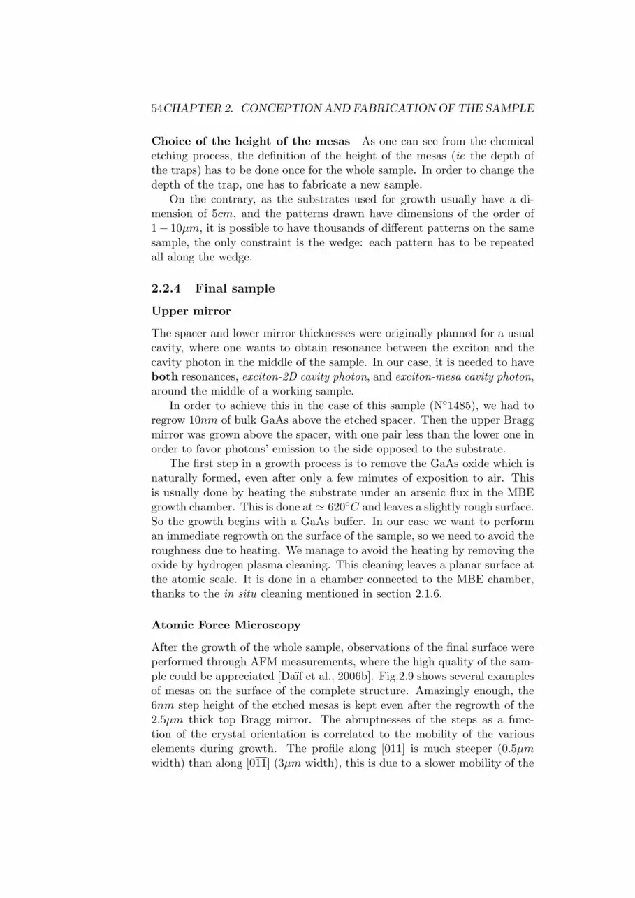
54CHAPTER 2. CONCEPTION AND FABRICATION OF THE SAMPLE
Choice of the height of the mesas As one can see from the chemicaletching process, the definition of the height of the mesas (ie the depth ofthe traps) has to be done once for the whole sample. In order to change thedepth of the trap, one has to fabricate a new sample.
On the contrary, as the substrates used for growth usually have a di-mension of 5cm, and the patterns drawn have dimensions of the order of1− 10µm, it is possible to have thousands of different patterns on the samesample, the only constraint is the wedge: each pattern has to be repeatedall along the wedge.
2.2.4 Final sample
Upper mirror
The spacer and lower mirror thicknesses were originally planned for a usualcavity, where one wants to obtain resonance between the exciton and thecavity photon in the middle of the sample. In our case, it is needed to haveboth resonances, exciton-2D cavity photon, and exciton-mesa cavity photon,around the middle of a working sample.
In order to achieve this in the case of this sample (N1485), we had toregrow 10nm of bulk GaAs above the etched spacer. Then the upper Braggmirror was grown above the spacer, with one pair less than the lower one inorder to favor photons’ emission to the side opposed to the substrate.
The first step in a growth process is to remove the GaAs oxide which isnaturally formed, even after only a few minutes of exposition to air. Thisis usually done by heating the substrate under an arsenic flux in the MBEgrowth chamber. This is done at' 620C and leaves a slightly rough surface.So the growth begins with a GaAs buffer. In our case we want to performan immediate regrowth on the surface of the sample, so we need to avoid theroughness due to heating. We manage to avoid the heating by removing theoxide by hydrogen plasma cleaning. This cleaning leaves a planar surface atthe atomic scale. It is done in a chamber connected to the MBE chamber,thanks to the in situ cleaning mentioned in section 2.1.6.
Atomic Force Microscopy
After the growth of the whole sample, observations of the final surface wereperformed through AFM measurements, where the high quality of the sam-ple could be appreciated [Daıf et al., 2006b]. Fig.2.9 shows several examplesof mesas on the surface of the complete structure. Amazingly enough, the6nm step height of the etched mesas is kept even after the regrowth of the2.5µm thick top Bragg mirror. The abruptnesses of the steps as a func-tion of the crystal orientation is correlated to the mobility of the variouselements during growth. The profile along [011] is much steeper (0.5µmwidth) than along [011] (3µm width), this is due to a slower mobility of the
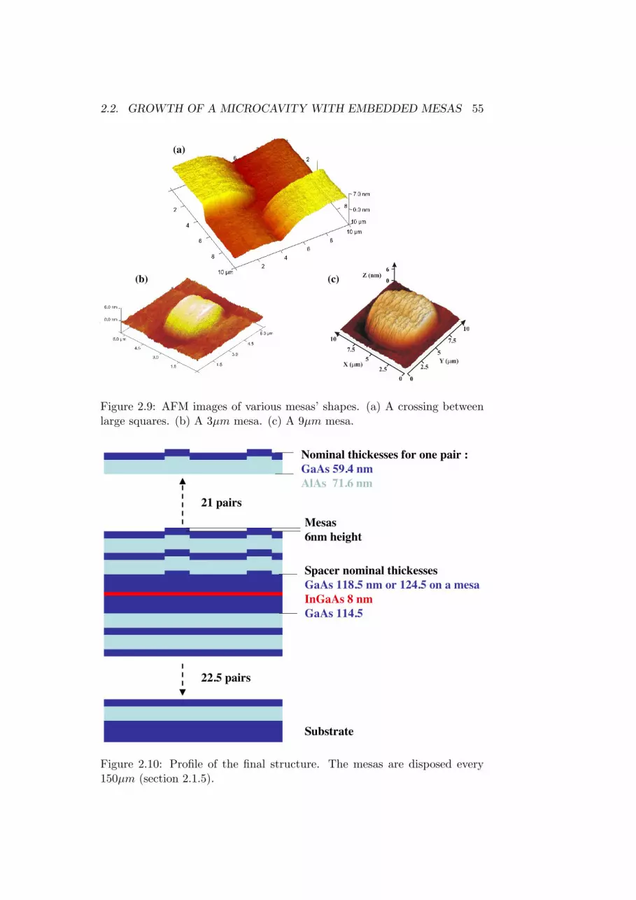
2.2. GROWTH OF A MICROCAVITY WITH EMBEDDED MESAS 55
(a)
(b) (c)
Figure 2.9: AFM images of various mesas’ shapes. (a) A crossing betweenlarge squares. (b) A 3µm mesa. (c) A 9µm mesa.
Substrate
Nominal thickesses for one pair :
GaAs 59.4 nm
AlAs 71.6 nm
Spacer nominal thickesses
GaAs 118.5 nm or 124.5 on a mesa
InGaAs 8 nm
GaAs 114.5
22.5 pairs
21 pairs
Mesas
6nm height
Figure 2.10: Profile of the final structure. The mesas are disposed every150µm (section 2.1.5).

56CHAPTER 2. CONCEPTION AND FABRICATION OF THE SAMPLE
atoms. This gives rise to a surface asymmetry along the different crystallineorientations, with a smoothing of the etched faces that increases propor-tionally to the overgrowth thickness, it is particularly visible on Fig.2.9(b),where the mesa had a diameter of 3µm at the spacer level.
As the cavity mode field extends only over the first pairs of the mirror(closest to the spacer layer [Savona et al., 1999]), the optical properties ofthe mesas will be weakly affected by this effect. Similar observations haverecently been reported for QDs embedded in similar mesas by ref [Lu et al.,2005], although the growth induced asymmetry seems to be much morepronounced, probably due to different growth conditions.
The step height measured by AFM corresponds to the height calculatedby transfer matrix simulations. We performed the transfer matrix simula-tions on and around mesas, and deduced the cavity mode energy on the 2zones, the difference between these 2 cavity modes gives the height of thestep. According to the AFM measurement on the top mirror of a 6nm step,we compute an energy difference of 9meV , in very good agreement with thephotoluminescence experiment results, as we will see in the next chapter.
The structure of the sample finally looks as shown on Fig.2.10.
2.3 Conclusion and improvement of the method
Let us see how some particular steps of the above described method couldbe improved, and conclude.
2.3.1 Step by step improvement
Lithography
As we saw in section 2.2.2, the optical method used to deposit the photore-sist pattern on the sample’s surface is subject to diffraction. Even if one canavoid some of these effects by making the photoresist layer as thin as pos-sible, this technique shows an intrinsic limitation because of the use of UVlight, which has a wavelength of the order of 0.4µm. Due to the diffractionlimit, it should not be possible to draw an object having a size smaller than≈ 2 ∗ a, a being the thickness of photoresist, so in the best case the smallestsize reachable is ≈ 0.5µm (the detailed calculation is performed in appendixB).
If one keeps this selective etching method, one possibility to overcomethe diffraction limit is the use of electron-beam lithography to deposit thepatterns on the sample’s surface. This method reaches a precision of theorder of 1− 10nm, far smaller than with UV photons.

2.3. CONCLUSION AND IMPROVEMENT OF THE METHOD 57
Use of AFM
One could imagine to use AFM at various steps of the growth and etchingprocess, instead of performing reflectivity measurements and simulations, inorder to check the etching process. This forces either to be able to performAFM measurements on a whole 2in wafer (not possible for us), or to performthe growth on small parts (but then attention has to be paid to the cleaningof the observed surfaces).
Nevertheless, if easily available, AFM will allow a faster characterizationof the step height, and will give an idea of the smoothness of the surface, ofthe steepness of the step...
Oxygen plasma
Instead of chemically etching the GaAs, one could pass it under oxygenplasma to oxide a given thickness, and then remove the oxide by simpleusual cleaning. This alternative method is only interesting if the calibrationof the oxidation time is better than the calibration of the chemical etchingtime.
2.3.2 Conclusion: a satisfactory sample
The method chosen to grow the sample allowed us to grow an original struc-ture. We will see in more detail in the next chapters its optical properties.We can nevertheless already say that, from a crystallographic point of view,it was a success. The surfaces show the smoothness of usual MBE grownGaAs structures, and the structures’ shapes were deposed as they were de-signed, and conserved along the regrowth process.

58CHAPTER 2. CONCEPTION AND FABRICATION OF THE SAMPLE

Part II
Physical studies
59


Chapter 3
Zero and two dimensionalstrong-coupling regimes
Our first aim after the realization of the sample is to characterize the cou-pling regime between the exciton and cavity photon modes. We will firsthave a look at the experimental methods we used, we will then see the resultsfor the 2D structure and finally for the 0D structure.
3.1 Experimental considerations
In order to observe the modes of the microcavity, several kinds of measure-ments are possible: reflectivity, transmission or luminescence measurementswill all give information.
Principles
White light reflectivity experiments consist of optically exciting the samplewith a wide range of energies, covering all the energies which are of interestin the frame of our study. The excitation is performed at extremely lowintensities, where no effect due to density is expected. The reflection ortransmission spectra are then studied and show the optical modes of thesystem. In particular, the photonic component of the polariton modes areobserved (as reflectivity dips or transmission peaks) in case of a microcavityshowing strong coupling regime.
Another possibility, as we are in presence of a system which shows energystates involving electronic excitations, is to populate the system at energieshigher than the energies of interest for us, namely the exciton and cavitymode energies. The excitation energy should be higher than the stopband’senergy, in order to efficiently couple to the system. The sample is pumped bya laser beam, showing low enough intensity not to induce nonlinearities. Thesystem relaxes then towards low energy states, and the latter (polaritons)
61

62CHAPTER 3. ZERO AND TWO DIMENSIONAL STRONG-COUPLING REGIMES
emit photons.
Spectrometer
Optical
filters
Sample
White light
F
D
•=F for laser excitation
•Sample conjugated with
the pinhole for white
light reflectivity
Cube
Lasers
Pinhole
500!m
Multimode
optical fibre
F
Gold mirror (if white
light illumination)
Diaphragm
Half reflecting
plate
Fiber holderFiber holder
Figure 3.1: Characterization setup. The sample’s plane is conjugated withthe pinhole for white light reflectivity, and placed at the focal length of thelens for a laser excitation. It is mounted on a submicron resolution 3D setof translations stages, the lenses, the cube and the pinhole are mounted on10µm resolution translation stages.
Experimental procedures
White light reflectivity The set-up used to perform such experimentsis shown on Fig.3.1. The source is a commercial white filament lamp, emit-ting with a black body spectrum at around 1500K. As the studied cavityshows patterns on its surface, the dimension of the shined surface must becontrolled carefully. The white light is focused on a pinhole which size ischosen to be 500µm and which acts as a secondary emitter. This allows usto choose the size of the excitation spot on the sample’s surface through agiven choice of the position of the pinhole-lens-sample ensemble. In orderto make a compromise between the patterns’ sizes (the squares are 300µmwide) and the unavoidable chromatic aberration, we chose the excitationspot to have a diameter of 100µm.
The lenses are achromatic lenses but given the wide range of wavelengthshined, chromatic aberrations are unavoidable. Hence, the spectrum illumi-
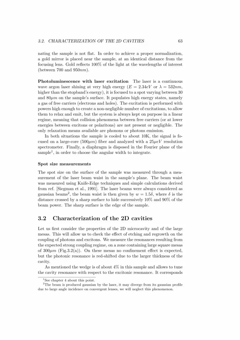
3.2. CHARACTERIZATION OF THE 2D CAVITIES 63
nating the sample is not flat. In order to achieve a proper normalization,a gold mirror is placed near the sample, at an identical distance from thefocusing lens. Gold reflects 100% of the light at the wavelengths of interest(between 700 and 950nm).
Photoluminescence with laser excitation The laser is a continuouswave argon laser shining at very high energy (E = 2.34eV or λ = 532nm,higher than the stopband’s energy), it is focused to a spot varying between 30and 80µm on the sample’s surface. It populates high energy states, namelya gas of free carriers (electrons and holes). The excitation is performed withpowers high enough to create a non-negligible number of excitations, to allowthem to relax and emit, but the system is always kept on purpose in a linearregime, meaning that collision phenomena between free carriers (or at lowerenergies between excitons or polaritons) are not present or negligible. Theonly relaxation means available are phonons or photons emission.
In both situations the sample is cooled to about 10K, the signal is fo-cused on a large-core (500µm) fiber and analyzed with a 25µeV resolutionspectrometer. Finally, a diaphragm is disposed in the Fourier plane of thesample1, in order to choose the angular width to integrate.
Spot size measurements
The spot size on the surface of the sample was measured through a mea-surement of the laser beam waist in the sample’s plane. The beam waistwas measured using Knife-Edge techniques and simple calculations derivedfrom ref. [Siegman et al., 1991]. The laser beams were always considered asgaussian beams2, the beam waist is then given by w = 1.5δ, where δ is thedistance crossed by a sharp surface to hide successively 10% and 90% of thebeam power. The sharp surface is the edge of the sample.
3.2 Characterization of the 2D cavities
Let us first consider the properties of the 2D microcavity and of the largemesas. This will allow us to check the effect of etching and regrowth on thecoupling of photons and excitons. We measure the resonances resulting fromthe expected strong coupling regime, on a zone containing large square mesasof 300µm (Fig.3.2(a)). On these mesas no confinement effect is expected,but the photonic resonance is red-shifted due to the larger thickness of thecavity.
As mentioned the wedge is of about 4% in this sample and allows to tunethe cavity resonance with respect to the excitonic resonance. It corresponds
1See chapter 4 about this point.2The beam is produced gaussian by the laser, it may diverge from its gaussian profile
due to large angle incidence on convergent lenses, we will neglect this phenomenon.

64CHAPTER 3. ZERO AND TWO DIMENSIONAL STRONG-COUPLING REGIMES
to an energy variation for the photonic resonance of about 50meV across thewhole sample. In the zone of interest this variation is about 2.4meV/mm.As we saw in the precedent chapter (section 2.1.3), the quantum well excitonis less affected by the wedge: its energy variation is below 3meV across thewhole sample.
300µm
6 nm
(a)
(b)
300µm
EX
Figure 3.2: (a) Pattern and thickness profile of a zone of squares. The entiremask was shown on Fig.2.4. The whole zone contains hundreds of squaredmesas. (b) Anticrossing curves obtained through reflectivity measurementsalong the wedge, successively on and outside squared mesas. The exciton’smean energy EX is indicated by a dashed line.
The spectral properties are studied through the two kinds of experimentspresented in the first section: photoluminescence and reflectivity. The mea-surements are performed every 300µm, alternatively on a mesa and betweentwo mesas. The profile of the surface is shown on Fig.3.2(a), where themesas are drawn in black, and the zones between mesas in grey.
The spectra show dips in the reflectivity stopband. The observed modesas a function of the position (and thus detuning between the exciton andphoton mode) are shown on Fig.3.2(b). Two anticrossing behaviors charac-teristic of a strong coupling regime can be seen. This is due to the presence oftwo cavity thicknesses showing two cavity modes: on the mesas and betweenmesas. The colors on the graph correspond to the colors on the pattern. Asexpected a mesa is higher physically but lower energetically.
In photoluminescence, the signal measured is a peak intensity at the

3.2. CHARACTERIZATION OF THE 2D CAVITIES 65
!E
!!
Figure 3.3: Anticrossing curves obtained through photoluminescence mea-surements. Arrows indicate the energy difference δE between the two cavitymodes and the Rabi splitting Ω.
modes of the cavity. We plotted the measured peaks’ energies as a functionof position on Fig.3.3. A similar double anticrossing behavior is measured.
Quantitative properties
We extracted the quantitative properties of the cavity from the PL spectra,considering that at such low temperatures (T ≤ 10K), the two reportedmethods show similar results. The microcavity shows a strong couplingregime and features a Rabi splitting energy of 3.5meV , and a full width athalf the maximum (FWHM) of γc = 220µeV for the cavity photon mode,corresponding to a quality factor of Q ' 7∗103, and of γX = 500µeV for thequantum well exciton. At resonance (δ = 0) the polariton linewidth is γLP '350µeV . These linewidths are slightly larger than reported in [Saba et al.,2000], which reports one of the best GaAs samples fabricated, and has avery similar structure. The latter shows γc = 100µeV , γX ' 150µeV . TheirRabi splitting is Ω = 3.6meV , in agreement with our present observations.
Cavity modes
The two cavity modes -on the mesas and around the mesas- are separatedby δE = 9meV . This can be measured through the difference betweenthe peaks far from resonance with the exciton, on Fig.3.3. This value ishence the energy depth of the trap formed by the mesas. According to ourtransfer matrix simulations, this energy difference corresponds to a thick-ness difference of 6nm between the two cavities, in agreement with the AFMmeasurements on the surface of the sample, and with the reflectivity mea-

66CHAPTER 3. ZERO AND TWO DIMENSIONAL STRONG-COUPLING REGIMES
surements performed at the surface of the spacer (after the chemical etching,see chapter 2).
The cavity mode shows the same linewidth on both domains. The twoanticrossings are identical, which guaranties that the etching process justshifts the cavity mode, and does not affect the quality factor.
3.3 Strong-coupling regime in zero dimension
We now focus on the effect of the confinement of the polaritons in circularmesas, through photoluminescence experiments3. The experimental con-ditions are similar to the ones described above, but the laser spot whichhas now a diameter of ' 17µm in order to enhance the mesa to 2D-cavityintensity ratio. These results were published in reference [Daıf et al., 2006b].
The spectra shown display both the mesa confined modes and the 2Dpolaritons of the planar cavity outside the mesa, displaced towards higherenergies. Let us note that the light emission from one single mesa is veryintense, which allowed us to perform all experiments on single mesas, wellbelow any nonlinear regime, in contrast to the case of pillar microcavities[Dasbach et al., 2001, Obert et al., 2004].
3.3.1 Strong-coupling in small mesas
The smallest circular mesas, where the confinement should be the strongest,have a diameter of 3µm, we will focus in this section on photoluminescence(PL) measurements performed on these mesas.
Photon confinement In order to probe first the confinement of the cavityphotons, we took spectra on mesas which cavity mode(s) is (are) expectedto be far from resonance with the exciton.
Fig.3.4(a) shows the spectrum of a mesa relatively far from resonance(the bottom of the photonic trap shows an energy 6meV smaller than the ex-citon energy). The lower polariton mode of the mesa is thus quasi-photonic.It is split into several peaks. For sake of clarity, we will first only considerthe ground level (G) and the first excited level (E1) (which is a doublet, wewill comment this further in the next section, 3.3.2) although more modesare visible. The quantized photonic peaks have a spectral width of about90µeV , a factor of two smaller than observed on the non-confined cavityphoton mode. The smallest value measured reached 70µeV , indicating aquality factor of Q ' 2.1 ∗ 104 for the confined photon modes (better thanfor the 2D photon modes, we will come back to this point in section 3.3.4).The energy of the confined ground level is 1.5meV above the energy of the
3Reflectivity experiments were carried out but given the small surface of the mesas,the signal to noise ratio was rather bad.
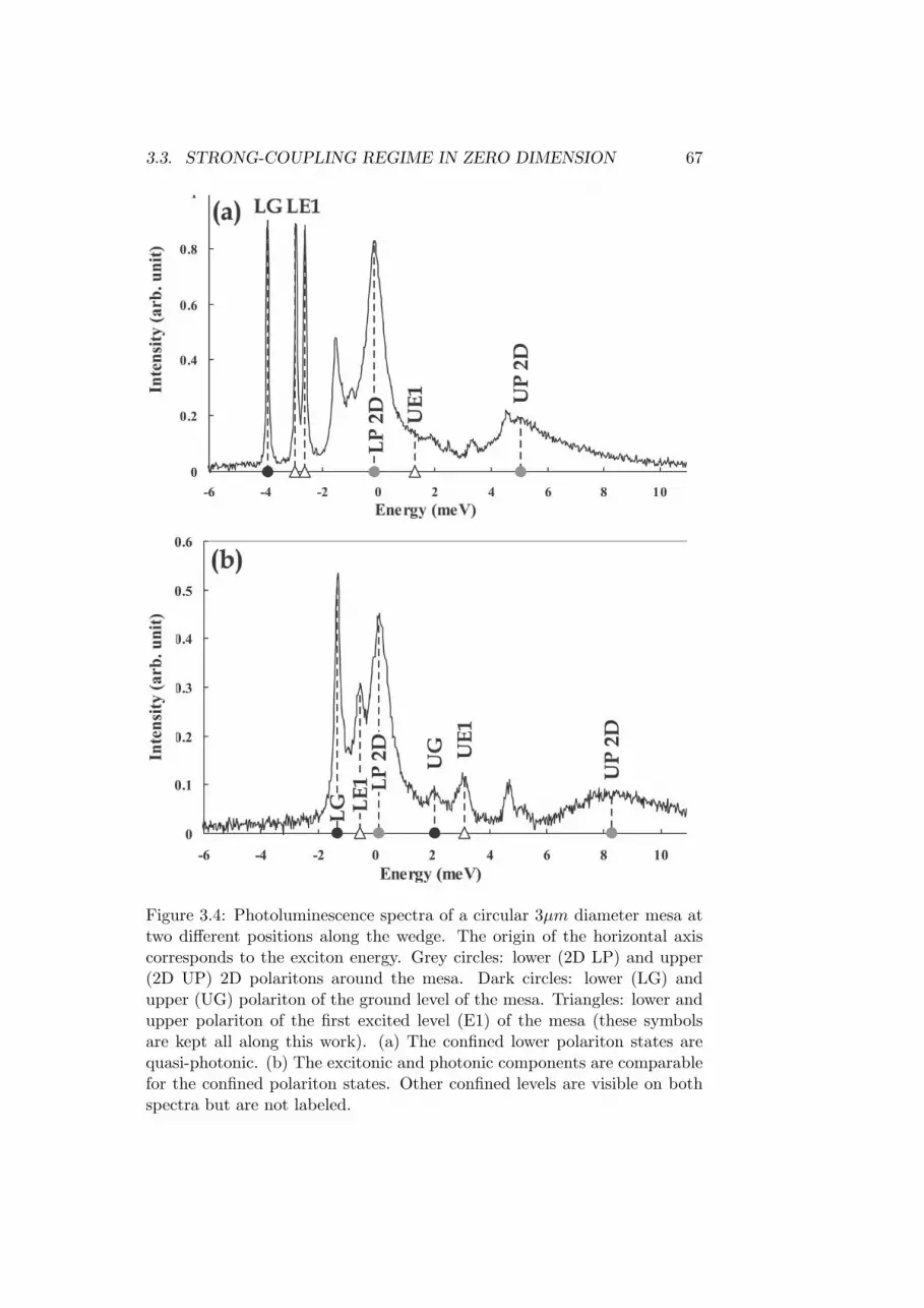
3.3. STRONG-COUPLING REGIME IN ZERO DIMENSION 67
where lower and upper polariton modes confined in thequantum box are nicely resolved. Despite the relatively largelinewidth of the 2D exciton, the high Q factor and thevery efficient relaxation to the quantum boxes allow one toobserve the confinement for both the lower and upperpolariton states.
In summary, we have reported the realization of a semi-conductor microcavity in strong coupling regime with em-bedded polariton quantum boxes. The trap consists of a mesain the spacer layer, obtained by a well controlled technique.Quantum confinement is resolved simultaneously for bothupper and lower polariton modes, and the anticrossing isresolved separately for all the quantized polaritons. Experi-mental and theoretical work on the dispersion of the quan-tized modes is being performed. The coexistence in the samesample of 2D and 0D polaritons, as well as the possibility tostudy a single quantum box, will allow original studies suchas resonant parametric scattering or trapping by spatial relax-ation. Wide possibilities in the transverse shape of the mesasalso open the way to the realization of various experimentalconfigurations for the bosonic polariton states, which energy,
wave function, and dimensionality can beengineered on demand.
The authors would like to acknowledge fruitful discus-sions with C. Ciuti, P. Lugan, M. Saba, and V. Savona. Theyare thankful for the strong financial support from the SwissNCCR research program Quantum Photonics.
1C. Weisbuch, M. Nishioka, A. Ishikawa, and Y. Arakawa, Phys. Rev. Lett.69, 3314 !1992".
2S. A. Moskalenko and D. W. Snoke, Bose-Einstein Condensation ofExcitons and Biexcitons and Coherent Nonlinear Optics with Excitons!Cambridge University Press, Cambridge, 2000".
3A. Kavokin, G. Malpuech, and F. P. Laussy, Phys. Lett. A 306, 187!2003".
4J. J. Baumberg, P. G. Savvidis, R. M. Stevenson, A. I. Tartakovskii, M. S.Skolnick, D. M. Whittaker, and J. S. Roberts, Phys. Rev. B 62, R16247!2000".
5M. Richard, J. Kasprzak, R. Romestain, R. André, and L. S. Dang, Phys.Rev. Lett. 94, 187401 !2005".
6J. P. Reithmaier, G. Sek, A. Löffler, C. Hoffmann, S. Kuhn,S. Reitzenstein, L. V. Keldysh, V. D. Kulakovskii, T. L. Reinecke, andA. Forchel, Nature !London" 432, 197 !2004".
7T. Yoshie, A. Scherer, J. Hendrickson, G. Khitrova, H. M. Gibbs,G. Rupper, C. Ell, O. B. Shchekin, and D. G. Deppe, Nature !London"432, 200 !2004".
8E. Peter, P. Senellart, D. Martrou, A. Lemaître, J. Hours, J.-M. Gérard, andJ. Bloch, Phys. Rev. Lett. 95, 067401 !2005".
9J. Bloch, F. Boeuf, J.-M. Gérard, B. Legrand, J.-Y. Marzin, R. Planel,V. Thierry-Mieg, and E. Costard, Physica E !Amsterdam" 2, 915 !1998".
10M. Obert, J. Renner, A. Forchel, G. Bacher, R. André, and D. L. S. Dang,Appl. Phys. Lett. 84, 1435 !2004".
11G. Dasbach, M. Schwab, and A. Forchel, Phys. Rev. B 64, 201309 !2001".12G. Dasbach, A. A. Dremin, M. Bayer, V. D. Kulakovskii, N. A. Gippius,
and A. Forchel, Phys. Rev. B 65, 245316 !2002".13R. P. Stanley, R. Houdré, U. Osterle, M. Gailhanou, and M. Ilegems, Appl.
Phys. Lett. 65, 15 !2004".14They have an elliptical shape with an absolute difference of about
0.75 !m between the small and the large axis. This asymmetry is given bythe pattern we designed on the photolithography mask.
FIG. 2. Photoluminescence spectra of a circular 3 !m diameter mesa at twodifferent positions: !a" x=1.04 and !b" x=4.42 !see Fig. 3". The origin of thehorizontal axis corresponds to the exciton’s energy. Grey circles: lower !2DLP" and upper !2D UP" 2D polaritons around the mesa. Dark circles: lower!LG" and upper !UG" polaritons of the ground level of the mesa. Triangles:lower and upper polaritons of the first excited level !E1" of the mesa. !a" LGand LE1 polariton states are quasiphotonic. !b" The excitonic and photoniccomponents are comparable for the confined polariton states. Other confinedlevels are visible on both spectra but are not labeled for sake of clarity.
FIG. 3. Energy of the photoluminescence peaks as a function of the spotposition along the wedge. Rabi splitting of 3.5 meV !3.35 meV" for the 2Dpolaritons !0D polaritons". !a" and !b" indicate the positions at which thespectra in Fig. 2 have been taken. Zero detuning for G !E1" around x=4.6 cm !x=3.05 cm".
061105-3 El Daïf et al. Appl. Phys. Lett. 88, 061105 !2006"
Downloaded 13 Feb 2006 to 128.178.175.4. Redistribution subject to AIP license or copyright, see http://apl.aip.org/apl/copyright.jsp
Figure 3.4: Photoluminescence spectra of a circular 3µm diameter mesa attwo different positions along the wedge. The origin of the horizontal axiscorresponds to the exciton energy. Grey circles: lower (2D LP) and upper(2D UP) 2D polaritons around the mesa. Dark circles: lower (LG) andupper (UG) polariton of the ground level of the mesa. Triangles: lower andupper polariton of the first excited level (E1) of the mesa (these symbolsare kept all along this work). (a) The confined lower polariton states arequasi-photonic. (b) The excitonic and photonic components are comparablefor the confined polariton states. Other confined levels are visible on bothspectra but are not labeled.

68CHAPTER 3. ZERO AND TWO DIMENSIONAL STRONG-COUPLING REGIMES
bottom of the trap (as measured on the large mesas at the same position onthe wedge).
Polariton confinement To probe the strong coupling in these mesas andthe polariton nature of the confined states, we systematically measured thespectra on mesas disposed along the wedge, so with different detunings withrespect to the exciton, the resulting curve is shown on Fig.3.5. On this setof measurements, we are always rather far from the position for which theexciton and 2D cavity mode are at resonance (We are at positions corre-sponding to 10mm < x < 15mm on Fig.3.2 and 3.3.). Hence, the 2D lowerpolariton mode stays near the exciton energy on the whole range of positionsshown in Fig.3.5.
Strong coupling is very nicely demonstrated for each confined state byan anticrossing behavior. They present a Rabi splitting of around 3.35meV ,it is identical for all the confined states, and fairly similar (though a slightlysmaller) than the 2D Rabi splitting of 3.5meV . Fig.3.4(b) displays thephotoluminescence spectrum very close to zero detuning in the trap, wherethe confined lower and upper polariton modes are resolved. Despite therelatively large linewidth of the 2D exciton, the high Q factor and the veryefficient relaxation to the traps allow to observe confinement for both thelower and upper polariton states.
Figure 3.5: Anticrossing for all confined states. Symbols of Fig.3.4 werekept. The exciton energy was chosen as the origin. The spectra on Fig.3.4were taken at: x = 1.04 (a) and x = 4.42 (b).

3.3. STRONG-COUPLING REGIME IN ZERO DIMENSION 69
Asymmetry of the anticrossing One can see that the anticrossingcurves are not symmetric with respect to the exciton energy: it was possibleto see the LP peaks at energies nearer to the exciton than the UP peaks.This is probably due to the broader linewidth of the upper polariton, and toa lower emission intensity, linked to its coupling with higher energy modes,and to its more numerous relaxation channels available (lower energy states).We will see a similar effect in the next section 3.3.2.
3.3.2 The doublet: a lift of degeneracy
As one can see on Fig.3.4 and 3.5, the confined first and second excited levelsappear as doublets on part of the measurements, this doublet is due to anasymmetry already present on the mask used for photolithography4. As weare in a 2-dimensional (x, y) system, the eigenstates Ex,y of the traps (herethe circular mesas) are linear combinations of eigenstates in each dimensionx or y of the plane:
• the ground state of the mesa is simply due to the combination betweenthe ground states in each dimension,
• the first excited state is due to a combination between the first excitedstate in one dimension x and the ground state in the other dimensiony, or the opposite combination of the ground x state and the excitedy state.
Therefore, if the two dimensions are different enough, it may lead toa splitting of the excited states due to both combinations. This splittingmust nevertheless not be considered as a polarization splitting, which isalso present (see for example [Sanvitto et al., 2005]) but which we did notobserve: when selecting a linear polarization in detection, we did not observeany significant sift of the peak energy.
One can see on Fig.3.5 that in certain conditions, it is not anymorepossible to see the splitting. Namely for the upper polariton of the confinedfirst excited state (triangles), and at positions above 2.75mm for the lowerpolariton’s first and second excited states. For all these situation the causeof the disappearance of the splitting is a spectral broadening of the modes.This broadening is due, for the lower polariton states, to their increasingexcitonic component when detuning is inscreased. As the exciton has aspectral linewidth of 500µeV , and the splitting is ≈ 300µeV , when the modeshows an excitonic Hopfield coefficient of more than 50%, its linewidth islarger than the splitting. For the upper polariton the main reason for thisbroadening is on one hand the coupling with the GaAs absorption band atslightly higher energy (' 1.52eV ) and on the other hand the numerous lowerenergy states towards which it can relax.
4described in the precedent chapter, section 2.1.5.

70CHAPTER 3. ZERO AND TWO DIMENSIONAL STRONG-COUPLING REGIMES
3.3.3 Larger mesas
We performed PL measurements in the same experimental conditions on9µm and 19µm-diameter mesas. As expected from traps with larger dimen-sions, the confined states energies get closer to each other with increasing thetrap size. It was thus not possible to follow the states’ energies as for thesmallest mesas, and perform anticrossing measurements. We neverthelessshow two PL spectra of 9µm mesas at two different exciton-photon detun-ings on Fig.3.6 and 3.7. The supposed positions of some modes are shownwith the same symbols used in the precedent figures.
Figure 3.6: PL of a 9µm mesa at very negative detuning for the confinedground state δ0D ' −5.5meV . The energies’ origin is chosen at the exciton’senergy.
Figure 3.7: PL of a 9µm mesa at a slight negative for the confined groundstate δ0D ' −2meV . The energies’ origin is chosen at the exciton’s energy.
One can see on Fig.3.6 the 2D polaritons, at rather high positive de-tuning, meaning that the upper polariton is mostly photon-like. The lat-ter is also very large spectrally, because of the combination of several fac-tors: its proximity with the GaAs absorption band at slightly higher energy

3.3. STRONG-COUPLING REGIME IN ZERO DIMENSION 71
(' 1.52eV ) and the numerous lower energy states towards which it can re-lax. Confined lower polariton states are on the opposite extremely sharpspectrally, with linewidths similar to what was observed for smaller mesas,around 80µeV . As a high number of confined modes is present, on canobserve on the same lower polariton the broadening of the peaks with in-creasing energy towards the exciton line.
On Fig.3.7 the ground mode of the mesa is closer to resonance with theexciton, and 2D polariton emission is on one hand dominated by the 0D LP(at the exciton energy) and on the other hand the photonic UP is at veryhigh energy. So only the signal due to the mesa is visible, and the peaks areclearly too wide to distinguish the quantization effect of confinement. Wewill see this point more in details when studying images.
3.3.4 Comment on the linewidths and high Q-factors
We mentioned in section 3.3.1 the fact that the confined cavity mode’slinewidth is smaller than that of the 2D, due to additional lateral confine-ment. One can be more precise by saying that this effect is a change in theinhomogeneous cavity mode linewidth, and that its homogeneous linewidthshould not be affected by the lateral confinement.
Two broadening factors in 2D are influenced by the confinement in themesas. These factors are in 2D:
• In case of a spatial detection with a resolution on a zone larger than≈ 10µm, inhomogeneous broadening due to disorder in the cavity[Savona, 2007].
• In case of a high spatial resolution in detection, resolution is lost inangle and thus in k−space. As the dispersion curve is parabolic-likearound normal incidence (~k|| = ~0), integrating PL on a large angularscale broadens the spectral linewidth.
In the present confinemed situation:
• The mesas studied have diameters of 3 and 9µm, they are thus notinfluenced by optical disorder. The fact that the 2D cavity feels thisdisorder does not affect the mesas’ modes, because their energy isdifferent from the 2D energy.
• PL signal coming from the confined modes shows no angular depen-dence of this energy. This means that there is no broadening of thepeak due to the angular loss of resolution.
Thanks to these two points, the linewidths measurement gets free fromtwo inhomogeneous optical broadening factors, and yields the observation ofa high Q-factor. The same results were obtained on photonic dots [Sanvitto

72CHAPTER 3. ZERO AND TWO DIMENSIONAL STRONG-COUPLING REGIMES
et al., 2005, Muller et al., 2006]. These dots were grown in similar ways,through a local thickness variation on the spacer of a 2D microcavity, andan improvement in the Q-factor was observed. The best Q-factor observedreached 30000.
As the confined polaritons linewidths is dominated by the radiative life-time, these values result in a polariton lifetime of ' 10ps yielded by theconfined photon lifetime. This is shorter than any other dephasing mecha-nism expected in this system at such low temperature and density.
3.4 Conclusion: a high quality confinement of stronglycoupled quasiparticles
The strong-coupling regime was demonstrated in all the available struc-tures: highly confining 0D structures and traditional 2D structures. Toour knowledge, this is the first time a single sample containing polaritons ofvarious dimensionality is realized. It is also the most non-ambiguous strong-coupling regime in 0D, with a high Rabi to linewidth ratio: Ω/γ ' 10 inthe 2D structures and ' 20 in the 0D structures. Several groups performedmicropillar-shaped microcavities showing strong-coupling regime between aquantum well excitons and confined photons, but either with difficulties toobserve a high Ω/γ ratio [Bloch et al., 1998], difficulties to observe the upperpolariton [Dasbach et al., 2001], or no mode splitting characteristic of theconfinement [Obert et al., 2004].
Another kind of 0D polaritons is being performed since a couple of yearsthrough another method: a confinement of electronic excitations in quantumdots [Peter et al., 2005, Reithmaier et al., 2004, Yoshie et al., 2004]. Thiskind of strong-coupling is different from what is described here, and theproblems and perspectives are also different. The difficulties are not asmuch in producing a high quality structure as they are in producing a highcoupling, through a suitable placing of the quantum dot inside the cavity,a problem for which a very clever solution was found by Badolato et al.,see Badolato et al. [2005]. This led them to a recent observation of thestrong-coupling regime between a single quantum dot and a photonic crystalnanocavity [Hennessy et al., 2007]. In these works perspectives are not on theside of collective effects, as the particle is by definition single, but towards thecontrol of single excitations in solid state, for various application (quantumcomputing, communication, cryptography) or fundamental studies.

Chapter 4
Spectroscopy of polaritons inthe real and reciprocal spaces
In order to fully characterize the confined polaritons, we imaged the po-lariton states’ photoluminescence (PL). Staying at excitation densities wellbelow any nonlinear threshold, we performed images in several configura-tions:
Spatially resolved spectroscopy Observation of the PL spectrum as afunction of one spatial dimension of the plane of the microcavity (x ory).
Angularly resolved spectroscopy Observation of the PL spectrum as afunction of one dimension of the reciprocal ( ~k||) space of the microcav-ity (kx or ky).
Two dimensional imaging 2D imaging either in real or reciprocal space.
4.1 Spectroscopy
4.1.1 Experimental setup
The experimental setup used to perform these various measurements isshown on Fig.4.1. It is designed to give an image of the surface of the sam-ple on the detector, in the real-space configuration, or of its Fourier plane,in the reciprocal space configuration, we will discuss further the notion ofFourier plane in the next paragraphs. The detectors are two CCD cameras:one imaging directly the two dimensions of the considered space (withoutspectral filtering), the other one is placed at the exit of a spectrometer,which selects one dimension and disperses it spectrally.
When imaging real space, the magnification is simply given by the ratiobetween the lens focusing on the CCD or spectrometer, and the microscopeobjective. As we worked with a microscope objective of NA 0.55 optimized
73

74CHAPTER 4. SPECTROSCOPY OF POLARITONS IN THE REAL AND RECIPROCAL SPACES
SpectrometerOptical filters
Microscope
objective
Sample
Held in
A cryostat
White light
Pellicule 4%
CCD with a 2D image
(real or reciprocal space)
•F=180mm for real space
imaging or
•d’ conjugated to d for
reciprocal space imagingFobj=4.5mm
E
xCube
d
Optical axis
Lasers
Lens
Focal length 80mm
Figure 4.1: Setup for imaging using non-resonant pumping.
for a magnification of 40, we chose the lens’s focal length to be 180mm,this yields a resolution limited by the diffraction of λ
2NA ' λ ' 0.8µm,and a scale of one pixel on the CCD array corresponding to 0.45µm on thesample’s surface.
The sample is held in a cold finger cryostat, cooled to ≈ 10K, andpumped (except for the last series of images) non-resonantly with an argonlaser, at very high energy (E = 2.34eV or λ = 532nm), the excitation spothas a diameter of ' 35µm.
Reflection Some images shown here were taken with a slightly differentset-up, where the excitation laser comes from the detection side. This im-poses to get rid of laser scattering with a spectral filter or a polarizer. Itdoes however not affect the image interpretation.
4.1.2 Reciprocal space spectroscopy
Principles
The space in which the eigenstates of the system are defined is the wavevector space. In order to see the wave function of the polaritons, it istherefore relevant to image the modes in this space. We will see in thissection how to access this space, through angle resolved measurements, andmeasure the dispersion curve of the polaritons.
Confined polaritons do not show the same dependency of the eigenstates:
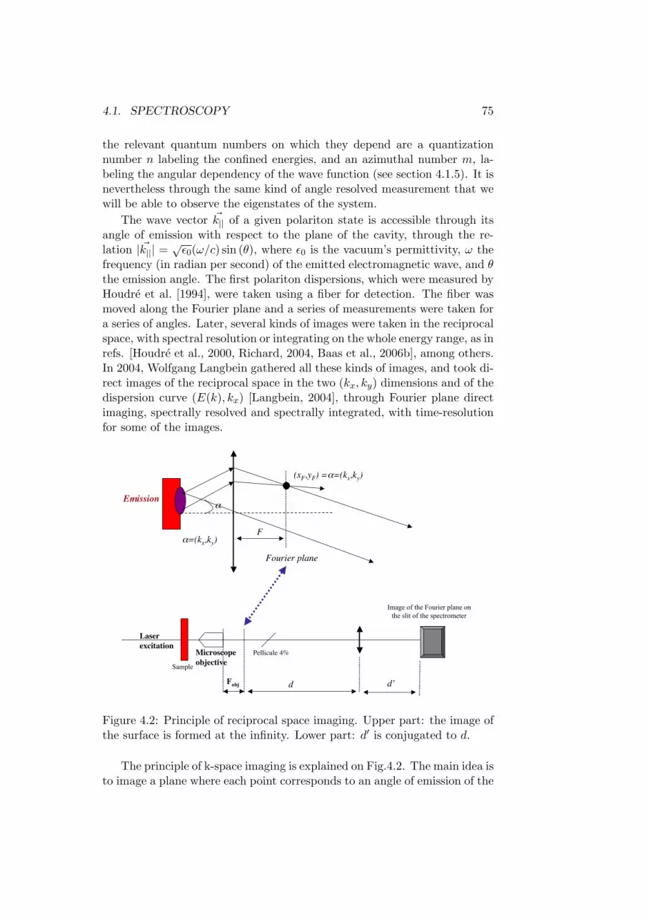
4.1. SPECTROSCOPY 75
the relevant quantum numbers on which they depend are a quantizationnumber n labeling the confined energies, and an azimuthal number m, la-beling the angular dependency of the wave function (see section 4.1.5). It isnevertheless through the same kind of angle resolved measurement that wewill be able to observe the eigenstates of the system.
The wave vector ~k|| of a given polariton state is accessible through itsangle of emission with respect to the plane of the cavity, through the re-lation | ~k||| =
√ε0(ω/c) sin (θ), where ε0 is the vacuum’s permittivity, ω the
frequency (in radian per second) of the emitted electromagnetic wave, and θthe emission angle. The first polariton dispersions, which were measured byHoudre et al. [1994], were taken using a fiber for detection. The fiber wasmoved along the Fourier plane and a series of measurements were taken fora series of angles. Later, several kinds of images were taken in the reciprocalspace, with spectral resolution or integrating on the whole energy range, as inrefs. [Houdre et al., 2000, Richard, 2004, Baas et al., 2006b], among others.In 2004, Wolfgang Langbein gathered all these kinds of images, and took di-rect images of the reciprocal space in the two (kx, ky) dimensions and of thedispersion curve (E(k), kx) [Langbein, 2004], through Fourier plane directimaging, spectrally resolved and spectrally integrated, with time-resolutionfor some of the images.
Image of the Fourier plane on
the slit of the spectrometer
Microscope
objectiveSample
Fobj
Pellicule 4%
d d’
Emission!
!=(kx,ky)
(xF,yF) =!=(kx,ky)
F
Fourier plane
Laser
excitation
Figure 4.2: Principle of reciprocal space imaging. Upper part: the image ofthe surface is formed at the infinity. Lower part: d′ is conjugated to d.
The principle of k-space imaging is explained on Fig.4.2. The main idea isto image a plane where each point corresponds to an angle of emission of the

76CHAPTER 4. SPECTROSCOPY OF POLARITONS IN THE REAL AND RECIPROCAL SPACES
cavity. Indeed, a parallel beam emitted by the sample is focused on a pointof the focal plane. This leads us to make the assumption that the emissionzone shows first-order phase coherence, otherwise the two mentioned beamswill simply see there intensities summed. More explanation about Fourieroptics for the same application can be found in the thesis of Maxime Richard[Richard, 2004] pp. 42 and following, and in references therein.
Results
Fig.4.3 shows dispersion curves for 3 mesa sizes at zero detuning for the 3µmmesa ground mode and slightly negative detunings for the 9µm and 19µmmesas. These images were taken by Reda Idrissi Kaitouni in collaborationwith Maxime Richard, and published in references [Kaitouni et al., 2006] and[Baas et al., 2006a]. They were taken in an experiment where excitation anddetection are situated on the same side of the sample, excitation is performedwith a 3µm spot. The dispersion of the extended polaritons (barely visiblein the 19µm mesa), is highlighted by dashed lines. We estimate a positivedetuning of 6.4meV between the extended 2D cavity mode and the exciton,it is hence a good approximation to consider the 2D lower polariton atthe exciton’s energy. The strongest PL signal appears on the three imagesbelow and above the 2D LP mode. In particular, on Fig.4.3(a), the 3µmmesa shows few discrete lines extending over broad angular regions, withenergy spacings in the meV range. Compared to the 3µm mesa, the 9µmmesa dispersion, shown on Fig.4.3(b) shows a larger number of more closelyspaced spectral lines, with a smaller angular spread. Finally, the 19µm mesadispersion, shown on Fig.4.3(c), shows a quasi-continuuous spectrum, whilethe angular extension is still smaller, approaching a 2D behavior.
Negative detuning Let us now see an example of dispersion we took atnegative detuning on Fig.4.4, the confined lower polariton is mostly photonicin this case. The 2D signal is here more intense than the 0D signal. Thecontrast has been enhanced by a factor of 50 for the confined lower polaritonto be visible. Relaxation is less efficient towards a photonic state.
One can see an unexpected signal at an energy of ≈ 1.50eV , this signal ischaracteristic of bulk GaAs polluted with carbon [Ilegems, 1985]. As thesemeasurements were taken in the usual transmission setup, the substrateis also excited by the laser. This peak is an indicator that the impurityconcentration has exceeded 1016impurities/cm3 (1), this is a reasonablenumber for commercial bulk GaAs. One can note the directionality of thisemission, centered around ~k|| = ~0, with secondary preferential axes at higherangles, we could not find any reason for this feature.
1As opposed to the high purity concentration of 1014impurities/cm3 reached for theGaAs grown by our MBE.

4.1. SPECTROSCOPY 77
88C
HA
PIT
RE
3.P
LD
EP
OLA
RIT
ON
S2D
&0D
!"!#$%&'(!)*
'+* ,&-
!./ / ./01-/
01-.
01-1
01-2
01--
013/
013.
0131
0132
013-
04//
+"$5!&'6!$#!!7*
'8* ,&..
!./ / ./
'9* ,&0.
!./ / ./
Fig. 3.5 – Photoluminescence d’une microcavité à plot dans l’espace réciproque pour des plots de 3, 9 et 19 µm dediamètre (de gauche à droite).Figure 4.3: Dispersion curves: Measured PL intensity (linear color scale fromblue to red) as a function of energy and emission angle for: (a) the 3µm, (b)the 9µm and (c) the 19µm mesa. Dashed lines: calculated dispersions ofthe extended polariton modes. These three experimental dispersion curvesare shown again on Fig.4.8 and compared with theory.
Angle (°)0 10 20
Ener
gy (
eV)
1020
1.480
1.485
1.490
1.475
30
x 50
1.500
1.495
1.505
Figure 4.4: Example of dispersion curve at negative detuning, for a 9µmmesa, in a transmission experiment. The angular window is not symmetricin order to allow the observation of large angles.

78CHAPTER 4. SPECTROSCOPY OF POLARITONS IN THE REAL AND RECIPROCAL SPACES
4.1.3 Real space spectroscopy
In order to perform real space spectroscopy, we simply image the surface ofthe sample on the entrance slit of the spectrometer, instead of the reciprocalspace, in order to see the density of polaritons in real space. In the case ofmesas, we are in presence of a confined system where the various states arediscrete in energy, thus the profile at a given energy is directly related to thepresence probability of the polariton at this energy, as a function of position.Similar images were taken for photonic dots in ref. [Lohmeyer et al., 2006].
Figure 4.5: Photoluminescence intensity as a function of energy and posi-tion for 3µm (a) and 19µm (b) diameter mesas. (a) For clarity, the intensityabove 1484.2 meV has been enhanced. The same symbols than in the prece-dent chapter are used to label the various states: grey circle for the 2Dpolaritons, black circle for the confined ground state, white triangle for theconfined first excited state, white rhombus for the confined second excitedstate. (b) The contrast is identical on the whole figure.
Fig.4.5(a) shows a spatially resolved spectrum of a 30µm long stripeof the sample surface (horizontal axis) containing a 3µm diameter mesa,non-resonantly excited through a 2µm diameter laser spot. The mesa isat a position along the wedge where the ground mode is at slight negativedetuning (δ ' −0.25meV ) with respect to the exciton. The stripe axis waschosen perpendicular to the wedge in order to prevent non-intrinsic sourcesof asymmetry. The luminescence emitted outside the mesa (delimited bythe dashed vertical lines) at 1483.8meV and 1490.5meV originates from the2D upper and lower polaritons at a positive detuning of δ = Ecav − Eexc '2ΩR. Note that the luminescence part of these modes situated inside the
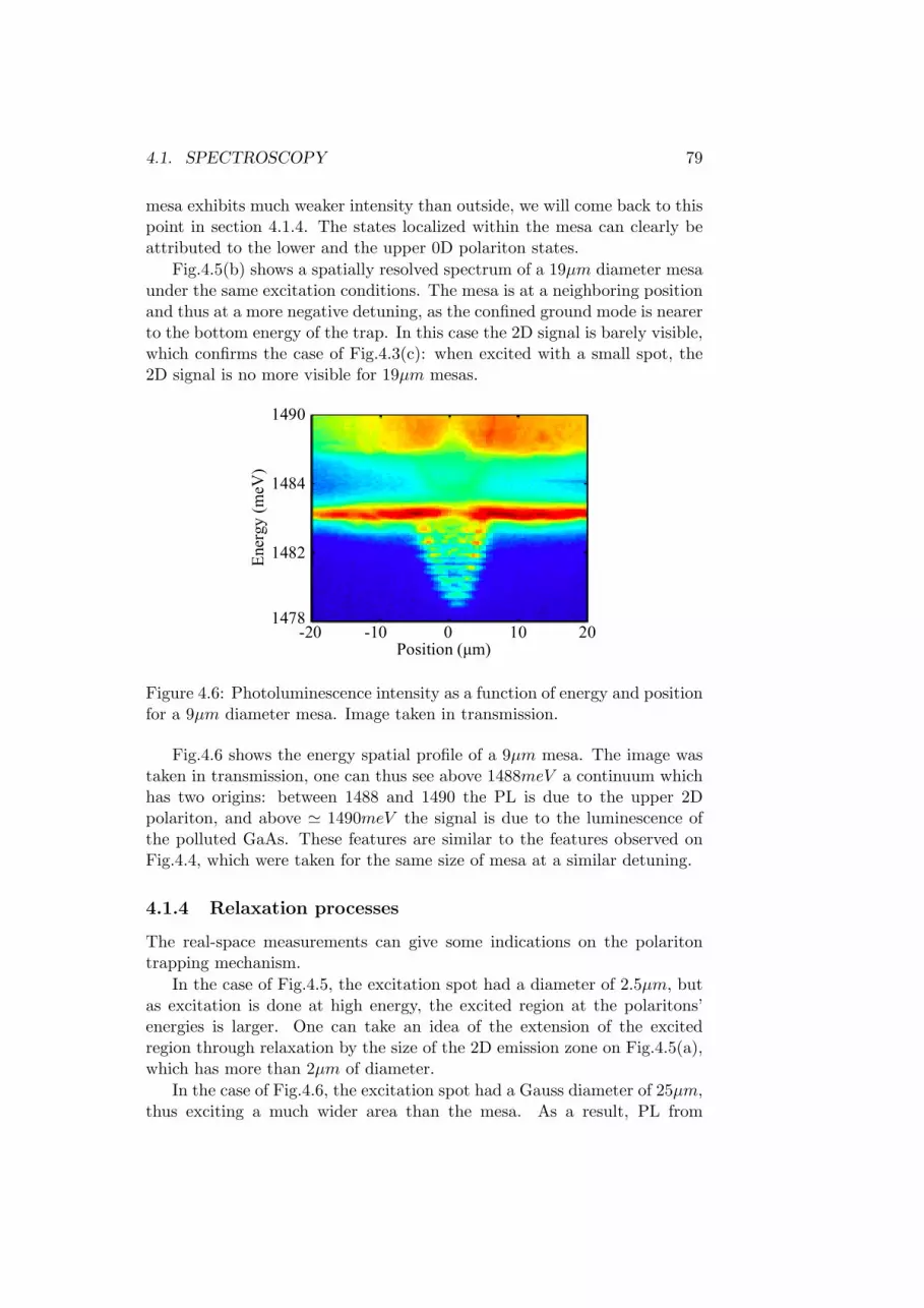
4.1. SPECTROSCOPY 79
mesa exhibits much weaker intensity than outside, we will come back to thispoint in section 4.1.4. The states localized within the mesa can clearly beattributed to the lower and the upper 0D polariton states.
Fig.4.5(b) shows a spatially resolved spectrum of a 19µm diameter mesaunder the same excitation conditions. The mesa is at a neighboring positionand thus at a more negative detuning, as the confined ground mode is nearerto the bottom energy of the trap. In this case the 2D signal is barely visible,which confirms the case of Fig.4.3(c): when excited with a small spot, the2D signal is no more visible for 19µm mesas.
Position (µm)0 10 20-10
1478
1482
1484
1490
Ener
gy
(m
eV)
-20
Figure 4.6: Photoluminescence intensity as a function of energy and positionfor a 9µm diameter mesa. Image taken in transmission.
Fig.4.6 shows the energy spatial profile of a 9µm mesa. The image wastaken in transmission, one can thus see above 1488meV a continuum whichhas two origins: between 1488 and 1490 the PL is due to the upper 2Dpolariton, and above ' 1490meV the signal is due to the luminescence ofthe polluted GaAs. These features are similar to the features observed onFig.4.4, which were taken for the same size of mesa at a similar detuning.
4.1.4 Relaxation processes
The real-space measurements can give some indications on the polaritontrapping mechanism.
In the case of Fig.4.5, the excitation spot had a diameter of 2.5µm, butas excitation is done at high energy, the excited region at the polaritons’energies is larger. One can take an idea of the extension of the excitedregion through relaxation by the size of the 2D emission zone on Fig.4.5(a),which has more than 2µm of diameter.
In the case of Fig.4.6, the excitation spot had a Gauss diameter of 25µm,thus exciting a much wider area than the mesa. As a result, PL from

80CHAPTER 4. SPECTROSCOPY OF POLARITONS IN THE REAL AND RECIPROCAL SPACES
the spatially-extended states is dominant. In general, however, confinedupper and lower polaritons are clearly visible in the three spectra. Andthey show a pattern which represents the spatial dependence of the squaredwave function of the polariton states. Some asymmetries can be seen, theyare probably due to the fact that the mesas are not perfectly circular. Wealso notice the irregular intensity pattern formed by the extended lowerpolariton branch, which is particularly evident in the 3 and 9µm spectra.The spatial fluctuations of the PL peak energy and the varying intensitysuggest the occurrence of weak spatial localization over a few tens of µm.This polariton localization is indeed expected in planar microcavities, dueto the intrinsic fluctuations of the cavity thickness produced in epitaxialgrowth (see ref. [Savona, 2007] and references therein).
2D-0D interaction... One can see on figures 4.5(a) and 4.6 that thesignal of the 2D polaritons is much weaker above the mesas. These intensity”holes” could be attributed to the efficient coupling between the 2D and 0Dpolariton states coexisting inside the mesa. In particular, the lower extendedpolariton (lower dashed line in Figs. 4.3) is almost fully exciton-like, witha vanishing photon component that results in a very long radiative lifetime.These states act as a reservoir from which polaritons relax into the confinedstates at lower energy. The relaxation can take place through interactionwith the thermal bath of phonons [Tassone et al., 1997], with free carriers,or via mutual polariton interaction [Porras et al., 2002].
...or a change in the density of states A competing interpretation is tosay that the density of 2D states decreases above the mesa. Simulations inreal space tend to validate this point of view, an example is shown on Fig.4.7,but it is not possible, from these measurements, do figure out whether thedecrease in PL intensity is more pronounced than the decrease in the densityof states... It is not possible with the present data to say which of twoprocesses is dominant.
4.1.5 Theoretical description of confined polaritons
In order to support the measured data, Pierre Lugan, Davide Sarchi andVincenzo Savona developed a theoretical model of trapped polaritons, pub-lished in refs. [Kaitouni et al., 2006, Lugan et al., 2006]. The model is basedon the re-writing in cylindrical coordinates of the 2D electromagnetic field,confined in circular mesas, and of the 2D free exciton wave function. We pro-vide the interested reader with a brief summary of this theory in appendixA. In this section we simply intend to compare the results of simulationsbased on this theory, to our experimental curves. One should mention thata theoretical article describing the case of cylindrical micropillar cavities waspublished by Panzarini and Andreani [1999], where the issue was different

4.1. SPECTROSCOPY 81
!30 !20 !10 0 10 20 30
1482
1484
1486
1488
1490
1492
1494
1496
radius (µm)
energ
y (
meV
)
Figure 4.7: Simulated spatial profile of the photon component of confinedand extended polaritons, in the case of a perfect circular mesa of 8.6µm indiameter. The modes shown are, from low to high energies: the confined LPground mode (blue), the confined LP fourth mode (red), an extended LPmode (green), the confined UP ground mode (magenta) and an extendedUP mode (clear blue).
as the leakage out of the cavity for small diameters had to be taken intoaccount.
Parameters used in the simulation The model described allows tosimulate the pattern of the measured spectra. For these simulations, circularmesas were assumed. The values of the diameter D and the detuning δbetween the 2D cavity mode and the exciton, used in the simulations, werefitted to the experimental data. For the 3, 9 and 19µm mesas these valuesare, respectively, D = 3.46, 8.6, and 20.0µm, and δ = 5.9, 6.8, and 7.1meV .For the remaining parameters, the nominal values of the sample were used.
Comparison Figs. 4.8 (d)-(f) display the simulated polariton spectraldensity for the three different mesas. Although the PL intensities in themeasured spectra (Figs. 4.8 (a)-(c)) account for the population of each state,it is not the case in the simulation as population densities are not taken intoaccount, and only the density of states are calculated. This implies thatit is not relevant to compare experimental and simulated intensities. Aslight discrepancy in the energies of the smallest mesa is probably due toits not perfectly circular shape. In general however, the model faithfullyreproduces both the energy position and angular extension of the variousspectral features.
We point out that the discrete modes in Fig.4.8(b) and (e), follow a pat-tern that mimicks the energy-momentum dispersion of 2-D polaritons. For

82CHAPTER 4. SPECTROSCOPY OF POLARITONS IN THE REAL AND RECIPROCAL SPACES
Gauss spot size was 25 !m, which excites an area largerthan the mesa and makes it possible to observe emission bothfrom spatially confined and extended states. As the distancebetween mesas is 125 !m, in each case a single mesa wasexcited.
III. PHOTOLUMINESCENCE MEASUREMENTS
When PL is measured from unprocessed regions far awayfrom the mesas, a typical spectrum of polaritons in a planarMC is observed. The measured vacuum field Rabi splitting is3.8 meV, with the extrapolated cavity-mode and excitonlinewidths being 200 and 500 !eV, respectively. Large pat-terned regions !250 !m"24 reveal a similar polariton disper-sion with a cavity mode energy 9 meV lower than in unproc-essed regions. This value is consistent with a "L=6 nmthickness variation from mesa to barrier, already pointed out.When the excitation spot is focused on one mesa, the PLspectrum shows discrete narrow lines, in addition to a weaksignature of the extended polariton states identical to thatmeasured in the unprocessed regions of the sample.
Real-space images give direct visual proof of polaritonconfinement. The deviations of the actual structure from aperfectly circular trap, however, result in confined states withslightly irregular shapes. Since only a narrow stripe is se-lected from the plane for imaging, the real-space informationmight not be directly comparable to the result of a model ofa perfectly circular trap. A more regular pattern is obtainedby measuring the amplitude of the polariton wave function inmomentum-space. We thus begin with the analysis ofmomentum-resolved spectra. As the polariton in-plane mo-mentum is related to the emission angle from the normalaxis, via the relation k=##0!$ /c"sin!%", we report directlythe angle-resolved spectral pattern. The measured patternsfor 3, 9, and 19 !m diameter mesas are displayed in Figs.2!a"–2!c". The dispersion of the extended polariton !barelyvisible in the 19 !m mesa" is highlighted by dashed lines.We estimate a positive detuning of 6.4 meV between theextended cavity mode and the exciton. The strongest spectralfeatures in the three images appear immediately below andabove the lower extended polariton mode. In particular, the3 !m mesa shows few discrete lines extending over broadangular regions, with energy spacings in the meV range. Thelinewidth of the lowest confined polariton level reaches70 !eV in this mesa, yielding a Q-factor as high as 21 000.This linewidth should be dominated by the polariton radia-tive rate, resulting in a polariton lifetime of 10 ps, stillshorter than any other dephasing mechanism expected in thissystem at low temperature and density. The fact that the con-fined polariton linewidth is smaller than one-half of thephoton-mode linewidth in the planar cavity suggests that thislatter is affected by some inhomogeneous broadening due tolong-range cavity thickness fluctuations. Compared to the3 !m mesa, the 9 !m one shows a larger number of moreclosely spaced spectral lines, with a smaller angular spread.Finally, in the 19 !m mesa these features approach a quasi-continuous spectrum, while the angular spread is stillsmaller.
Figures 3!a"–3!c" show three PL spectral patterns in real-space, for the 3, 9, and 19 !m mesa, respectively. These
spectra were obtained by excitation with a spot diameterlarger than the mesas. The spectrum for the 3 !m mesa inFig. 3!a" was taken at a detuning comparable to that of Fig.2!a", whereas for the two other mesas in Figs. 3!b" and 3!c"a detuning close to zero for the extended modes was chosen.Again, as for the momentum-space images, confined and ex-tended spectral features of both upper and lower polaritons
FIG. 2. !Color online" !Left" Measured polariton PL intensity!linear color scale from blue to red" as a function of energy andemission angle for the 3 !m !a", 9 !m !b", and 19 !m !c" mesa.For clarity, the intensity above 1485 meV is multiplied by a con-stant factor, as indicated. Dashed: dispersion of the extended polar-iton modes, computed from a coupled oscillator model. !Right" In-tensity plot of the simulated polariton spectral density for the 3 !m!d", 9 !m !e", and 19 !m !f" mesa !color log-scale, 4 decades fromblue to red".
ENGINEERING THE SPATIAL CONFINEMENT OF… PHYSICAL REVIEW B 74, 155311 !2006"
155311-3
Figure 4.8: Left-hand column: Measured polariton PL intensity (taken fromFig.4.3) as a function of energy and emission angle for: (a) the 3µm, (b) the9µm and (c) the 19µm mesa. Dashed: dispersion of the extended polaritonmodes, computed from a coupled oscillator model. Right-hand column:Intensity plot of the simulated polariton radiative spectrum for: (d) the3µm, (e) the 9µm and (f) the 19µm mesa (color log-scale, 4 decades fromblue to red). Figure taken from ref. [Kaitouni et al., 2006]. Courtesy ofVincenzo Savona.

4.1. SPECTROSCOPY 83
diameters larger than 20 µm, the simulation results in a spectrum practi-cally identical to that of 2D polaritons in a microcavity of thickness equalto that of the 2D cavity plus the mesa height.
4.1.6 Conclusion
We performed a spectroscopy of the confined and extended polaritons’ wavefunctions profile in photoluminescence, in the relevant configurations: en-ergy as a function of the reciprocal space and of the real space. The 0Dcharacter of the confined polaritons is confirmed by the angular width of theconfined states. The real space spectroscopy allowed us to directly probethe wave function profile with optical imaging, a quite unique situation insuch systems, allowed by the very low effective mass of polaritons.

84CHAPTER 4. SPECTROSCOPY OF POLARITONS IN THE REAL AND RECIPROCAL SPACES
4.2 2D images through resonant excitation
We saw, in the first part of this chapter, measurements of the eigenenergiesof the system we are studying as a function of one dimension of its reciprocalor real spaces. This allowed us to observe the wave function profile, but didnot allow us to observe in particular the potential effect of asymmetries of themesas. This needs a 2D imaging in both spaces. We performed such imagesthrough a quite unusual method we will develop in the first section, we willthen present the results2 and finally propose some possible interpretations.
4.2.1 Set-up
We excited resonantly (in angle and energy) at extremely low pump powera given state of the system. For this purpose we performed small changesin the set-up described in the precedent section, the present set-up is shownon Fig.4.9. Imaging is performed in transmission with respect to the laser.The excitation was performed with a TiSa continuous laser, focused to aspot of ' 35µm in diameter.
Spectrometer
Microscope
objective
White light
Pellicule 4%Cube
d
Optical axis
Photographic
objective
Lasers
Retroreflector:
Allows a change in
the excitation
angle
CCD with a 2D image
(real or reciprocal space)
Sample
Held in
A cryostat
Fobj=4.5mm
•F=180mm for real space
imaging
or
•d’ conjugated to d for
reciprocal space imaging
Figure 4.9: Setup for resonant excitation.
2Nota bene: as it is important that each image and its corresponding comments areseen on the same page, we will repeatedly insert page breaks till the end of this chapter.
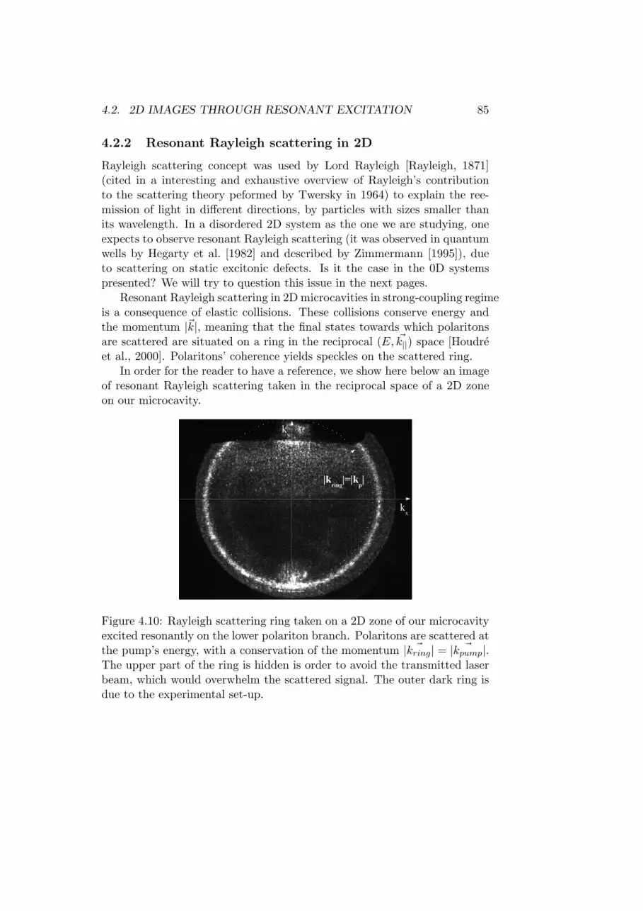
4.2. 2D IMAGES THROUGH RESONANT EXCITATION 85
4.2.2 Resonant Rayleigh scattering in 2D
Rayleigh scattering concept was used by Lord Rayleigh [Rayleigh, 1871](cited in a interesting and exhaustive overview of Rayleigh’s contributionto the scattering theory peformed by Twersky in 1964) to explain the ree-mission of light in different directions, by particles with sizes smaller thanits wavelength. In a disordered 2D system as the one we are studying, oneexpects to observe resonant Rayleigh scattering (it was observed in quantumwells by Hegarty et al. [1982] and described by Zimmermann [1995]), dueto scattering on static excitonic defects. Is it the case in the 0D systemspresented? We will try to question this issue in the next pages.
Resonant Rayleigh scattering in 2D microcavities in strong-coupling regimeis a consequence of elastic collisions. These collisions conserve energy andthe momentum |~k|, meaning that the final states towards which polaritonsare scattered are situated on a ring in the reciprocal (E, ~k||) space [Houdreet al., 2000]. Polaritons’ coherence yields speckles on the scattered ring.
In order for the reader to have a reference, we show here below an imageof resonant Rayleigh scattering taken in the reciprocal space of a 2D zoneon our microcavity.
ky
kx
|kring|=|k
p|
Figure 4.10: Rayleigh scattering ring taken on a 2D zone of our microcavityexcited resonantly on the lower polariton branch. Polaritons are scattered atthe pump’s energy, with a conservation of the momentum | ~kring| = | ~kpump|.The upper part of the ring is hidden is order to avoid the transmitted laserbeam, which would overwhelm the scattered signal. The outer dark ring isdue to the experimental set-up.

86CHAPTER 4. SPECTROSCOPY OF POLARITONS IN THE REAL AND RECIPROCAL SPACES
4.2.3 Images of a 9 micron mesa
In order to recall the spectrum of the 9µm mesa studied, its 2D and 0Dlower polaritons spatial and angular profiles are shown on Fig.4.11, througha non-resonant pumped PL experiment.
1.485
1.483En
erg
y (
eV
)
1.484
Position (µm) Angle (°)
0 10 20 30 40 50 60 70 80 90
35 45 55
-10 0 10
-10 0 10
35
45
55
10
0
-10
1.482
(a) (b)
(b)(a)
Ang
le (°)
Po
siti
on (
µm
)
Position (µm) Angle (°)
1.485
1.483Energ
y (
eV)
1.484
1.482
Angle (°)
-10 0 10
Figure 4.11: A 9µm-mesa. PL images of (a) the energy as a function of onespatial dimension, (b) the energy as a function of the angle. Only the lowerpolaritons are shown.
A specific angle-energy couple was chosen to excite resonantly a stateobserved on the dispersion curve. Nevertheless, the laser is probably notperfectly mode-matched with the excited mode, as the laser electromagneticmode can not be adapted to the polariton mode.
We pumped a 9µm mesa at δ0D ' 0 with an angle of 7 at 1.4831eV . Themeasured PL intensity is mostly emitted at the pumped energy, as can beseen on Fig.4.12, where the dispersion curve of the confined lower polaritonis shown when pumped resonant on the fourth confined LP state.
1.485
1.483En
erg
y (
eV
)
1.484
Position (µm) Angle (°)
0 10 20 30 40 50 60 70 80 90
35 45 55
-10 0 10
-10 0 10
35
45
55
10
0
-10
1.482
(a) (b)
(b)(a)
Ang
le (°)
Po
siti
on (
µm
)
Position (µm) Angle (°)
1.485
1.483Energ
y (
eV)
1.484
1.482
Angle (°)
-10 0 10
Figure 4.12: Lower polariton dispersion when pumped resonantly on thefourth confined LP state (third excited state). The pump energy is clearlyseen just above 1483meV thanks to laser scattering. But the transmittedlaser can not be seen as the reciprocal plane line imaged does not containthe incident laser beam. The latter does not hit the slit of the spectrometer.
We performed in this configuration 2D images in the real and reciprocalspaces, shown on Fig.4.13(a) and (b). One can see on both images 6 emis-sion lobes, periodically disposed in angle, though one is less intense. Theselobes are the maxima of the squared excited wave function in real and recip-rocal spaces, but so far one can not discriminate whether this wave functiondescribes an eigenstate of the system or a superposition of eigenstates, we

4.2. 2D IMAGES THROUGH RESONANT EXCITATION 87
will discuss this further at the end of the chapter.
1.485
1.483En
erg
y (
eV
)
1.484
Position (µm) Angle (°)
0 10 20 30 40 50 60 70 80 90
35 45 55
-10 0 10
-10 0 10
35
45
55
10
0
-10
1.482
(a) (b)
(b)(a)
Ang
le (°)
Po
siti
on (
µm
)
Position (µm) Angle (°)
1.485
1.483Energ
y (
eV)
1.484
1.482
Angle (°)
-10 0 10
Figure 4.13: A 9µm-mesas resonantly pumped with an angle of 7 at1.4831eV (as shown on Fig.4.12 and indicated by the dashed red lines onFig.4.11). (a) The 2 planar spatial dimension. (b) The 2 reciprocal spacedimensions, the laser beam incident direction is shown by a red circle.
It is remarkable that the laser can not be distinguished from the PLsignal. In particular on the reciprocal space images (Fig.4.13(b)), it wouldbe impossible to guess which reciprocal space point (kx, ky) is excited if itwas not indicated by the red circle.
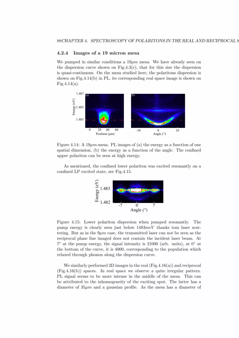
88CHAPTER 4. SPECTROSCOPY OF POLARITONS IN THE REAL AND RECIPROCAL SPACES
4.2.4 Images of a 19 micron mesa
We pumped in similar conditions a 19µm mesa. We have already seen onthe dispersion curve shown on Fig.4.3(c), that for this size the dispersionis quasi-continuous. On the mesa studied here, the polaritons dispersion isshown on Fig.4.14(b) in PL, its corresponding real space image is shown onFig.4.14(a).
1.483
1.485
1.487
En
ergy
(eV
)
-10 0 10Angle (°)
-7 0 7
Position (µm)
20 40 600
20 40
20
40
7
0
-7
(d)
(b)(a)
(b)
Ang
le (°)
Po
siti
on (
µm
)
Angle (°)
Position (µm)
-7 0 7Angle (°)
1.483
1.482En
erg
y (
eV)
Figure 4.14: A 19µm-mesa. PL images of (a) the energy as a function of onespatial dimension, (b) the energy as a function of the angle. The confinedupper polariton can be seen at high energy.
As mentioned, the confined lower polariton was excited resonantly on aconfined LP excited state, see Fig.4.15.
1.483
1.485
1.487
En
ergy
(eV
)
-10 0 10Angle (°)
-7 0 7
Position (µm)
20 40 600
20 40
20
40
7
0
-7
(d)
(b)(a)
(b)
Ang
le (°)
Po
siti
on (
µm
)
Angle (°)
Position (µm)
-7 0 7Angle (°)
1.483
1.482En
erg
y (
eV)
Figure 4.15: Lower polariton dispersion when pumped resonantly. Thepump energy is clearly seen just below 1483meV thanks tom laser scat-tering. But as in the 9µm case, the transmitted laser can not be seen as thereciprocal plane line imaged does not contain the incident laser beam. At7 at the pump energy, the signal intensity is 21000 (arb. units), at 0 atthe bottom of the curve, it is 4000, corresponding to the population whichrelaxed through phonon along the dispersion curve.
We similarly performed 2D images in the real (Fig.4.16(a)) and reciprocal(Fig.4.16(b)) spaces. In real space we observe a quite irregular pattern.PL signal seems to be more intense in the middle of the mesa. This canbe attributed to the inhomogeneity of the exciting spot. The latter has adiameter of 35µm and a gaussian profile. As the mesa has a diameter of

4.2. 2D IMAGES THROUGH RESONANT EXCITATION 89
1.483
1.485
1.487
En
ergy
(eV
)
-10 0 10Angle (°)
-7 0 7
Position (µm)
20 40 600
20 40
20
40
7
0
-7
(d)
(b)(a)
(b)
Ang
le (°)
Po
siti
on (
µm
)Angle (°)
Position (µm)
-7 0 7Angle (°)
1.483
1.482En
erg
y (
eV)
Figure 4.16: A 19µm-mesas resonantly pumped with an angle of 7 at1.4831eV (as shown on Fig.4.15 and indicated by the dashed red lines onFig.4.14). (a) The 2 planar spatial dimension. (b) The 2 reciprocal spacedimensions, the laser beam incident direction is shown by a red circle.
19µm, its surface can not be considered negligible compared to the spot’ssurface. We may therefore be exciting and observing a superposition ofstates showing a higher amplitude in the center of the mesa.
The 2D reciprocal space image (Fig.4.16(b)) is less regular and periodicthan in the 9µm diameter mesa case. We nevertheless observe a ring withintense regular patterns which are very different from the speckles observedon Fig.4.10. One can also see a rich signal at angles smaller than the pumpangle of 7. As there is no spectral filtering, it can be attributed to lowerenergy signal or to lobes of the excited confined state. Fig.4.15 shows thedispersion curve with the resonant excitation. It is difficult to discriminatebetween the two sources which probably both contribute to the signal...

90CHAPTER 4. SPECTROSCOPY OF POLARITONS IN THE REAL AND RECIPROCAL SPACES
4.2.5 Images of a 3 micron mesa
We also pumped the smallest mesas in similar conditions. Its lower polaritonenergy profile is shown. A technical problem of the pump laser made itimpossible to pump the first excited level of the mesa.
We thus pumped the ground level, as indicated by red dashed lines onFig.4.18(a) and (b), on a figure taken under non-resonant excitation.
834.6à836.4nm
1.483
1.485
Energ
y (
eV)
-10 0 10Angle (°)
-5 0 5
Position (µm)
0 5 10 15 20
7 10 13
7
10
13 -5
0
5
(a) (b)
(a) (d)
Ang
le (°)
Po
siti
on
(µ
m)
Angle (°)Position (µm)
(b)
Figure 4.17: A 3µm-mesa. PL images of (a) the energy as a function of onespatial dimension, (b) the energy as a function of the angle (or one reciprocalspace dimension). Only the lower polaritons are shown.
As expected this level simply shows a single lobe in both real and recip-rocal spaces, as shown on Fig.4.18.
834.6à836.4nm
1.483
1.485
Energ
y (
eV)
-10 0 10Angle (°)
-5 0 5
Position (µm)
0 5 10 15 20
7 10 13
7
10
13 -5
0
5
(a) (b)
(a) (d)
Ang
le (°)
Po
siti
on
(µ
m)
Angle (°)Position (µm)
(b)
Figure 4.18: A 3µm-mesas resonantly pumped with an angle of 7 at1.4827eV (as shown by the dashed red lines on Fig.4.17). (a) Energy asa function of one spatial dimension, (b) Energy as a function of the angle(or one reciprocal space dimension).
Here again one can note that it is absolutely impossible to distinguishthe laser beam from the mesa signal.

4.2. 2D IMAGES THROUGH RESONANT EXCITATION 91
4.2.6 Interpretation
Let us propose now an interpretation of our observations in 0D, and a linkbetween the 2D and 0D cases.
Rayleigh or not?
Let us first focus on the 9µm mesa. In both real and reciprocal spaces,resonant excitation of a given state allowed us to observe what seems to bea single state, without performing any spectral filtering.
This state has 6 lobes in both spaces, as Fig.4.13 shows, it is thereforelikely to be a state showing an azimuthal number m = 3. For a perfectcircular symmetry, the latter is degenerate into values ranging between mn =−3 and mn = +3. As we are not in a case of perfectly circular mesas, there iscertainly a lift of degeneracy between mn = ±1, ±2, and ±3, yielding energydifferences larger than the laser’s linewidth. These states show |2mn| lobes,thus we should be observing a state showing mn = ±3. Each of these singlequantum states probably see its lobes’ positions defined by the asymmetriesof system: crystalline axes, rough round interface of the mesa...
It is likely that we are exciting a linear combination of these two states,precisely the combination showing a lobe corresponding to the laser’s in-cidence angle. The mechanism through which we see this state is thus amode-matching mechanism, and not Rayleigh scattering. An experimentwhich will allow to validate this interpretation is be to turn the laser’s inci-dence on the same solid angle.
One could however be more general in the interpretation: the excitationis performed through a laser showing a certain profile in k-space, this profilecorresponds to a certain combination in the (n, m) space (see appendix Aabout the quantum numbers), and this combination does not necessarilyincludes states sharing the same quantum number n.
In order to check this possibility a theoretical calculations of the modesfor perfectly circular mesas of several diameters 8, 8.6 and 9µm is shownon Fig.4.19. As we already saw in chapter 2, the mesas are not perfectlycircular, but elliptic. Their energies are therefore a superposition of circularmesas’ energies. On Fig.4.19, the two lines at energies E and E′ are guide-to-the eye lines showing that several states (belonging to the same size or todifferent sizes) share very close energies. It is thus likely that a combinationincluding several (n, m) states is excited.
Broader mesa and transition to 2D Despite the fact that its dispersioncurve on Fig.4.14 is hard to differentiate from a 2D continuous dispersion,one can see that the 19µm mesa signal in reciprocal space, while excitedresonantly (Fig.4.15 and 4.16), shows a profile clearly different from the 2DRayleigh scattering shown on Fig.4.10. It seems to have 10 lobes, corre-

92CHAPTER 4. SPECTROSCOPY OF POLARITONS IN THE REAL AND RECIPROCAL SPACES
E'
EE
8µm 8.6µm 9.2µm
Figure 4.19: Energy of the modes in the (n, m) space. For each value of m,the states are labeled with an increasing number n with increasing energy.The fourth state in terms of growing energy for the 8.6µm mesa is indicatedby the black dashed line, the state showing m = 3 for the same mesa isindicated by the grey dashed line.
sponding to mn = ±5. So we are probably again exciting a combination ofstates showing the same energy, and this combination shows on of the lobesat the incidence angle of the laser, as in the 9µm case.
Increasing the mesa size brings more (n, m) states to be involved in thesuperposition of states necessary for the laser to couple into the system, theresulting superposition shows thus narrower angular lobes. Going towardsthe 2D limit, this superposition’s result is reduced to one lobe, and this lobe’sangular width is reduced when the number N of states involved increases. Itdefines the angular width of the transmitted laser, which is usually smallerthan the incident one.
And where is the Lord? It is difficult to figure out at which confine-ment diameter Rayleigh scattering begins to play a role. As one can seeon Fig.4.16, the emission pattern is not regular for a 19µm mesa, it is thuslikely that other states were populated, with neighboring energies, throughRayleigh scattering. But this mechanism does nevertheless not seem to bedominant, as th main pattern shows clear periodical lobes.
The latter case is to be opposed with the 2D case on Fig.4.10, whereRayleigh scattering clearly dominates and populates a whole ring in k-space,made of a high number of states.
Impact of disorder: Rayleigh scattering is related to disorder, that hastwo sources: cavity or exciton disorder.

4.2. 2D IMAGES THROUGH RESONANT EXCITATION 93
1. For small mesas with diameters . 10µm, confinement and quantiza-tion of the energies renders the states insensitive to photon disorder,which in addition is present on larger typical lengths (> 10µm). Whenincreasing the size of the mesa, the dispersion gets quasi-continuousand the diameter becomes larger to the typical size (≈ 10µm) of thephotonic disorder in a GaAs cavity. It is thus possible that this disor-der starts to play a minor role for the 19µm diameter mesa, while itplays an important role in the broadening of the linewidths in the 2Dstructure.
2. On the other hand, exciton disorder shows a typical size of the order of10−100nm. Collisions of polaritons on these static defect (that wouldbe Rayleigh scattering) can not play a role in this discrete system asno states towards which polariton could scatter are available. Again,when increasing the confinement size, states at similar energies thanthe pumped state appear, and Rayleigh scattering can play a role.
4.2.7 Conclusion
In conclusion we propose here an innovative spectroscopy technique throughresonant pumping. We directly observe the wave function of a superpositionof confined states and their Fourier transform. It is a quite unique situationat such scales in a quantum system, possible thanks to the exceptionallysmall mass of the polaritons.
We point out the question of the transition between two situations: aconfined situation where a single quantum state is excited, and a situa-tion where a continuum of states is available, and populated (excited) byRayleigh scattering. We proposed some possible answers, further experi-ments through variation of the excitation conditions, may give some moreclues to understand further and situate this transition.

94CHAPTER 4. SPECTROSCOPY OF POLARITONS IN THE REAL AND RECIPROCAL SPACES
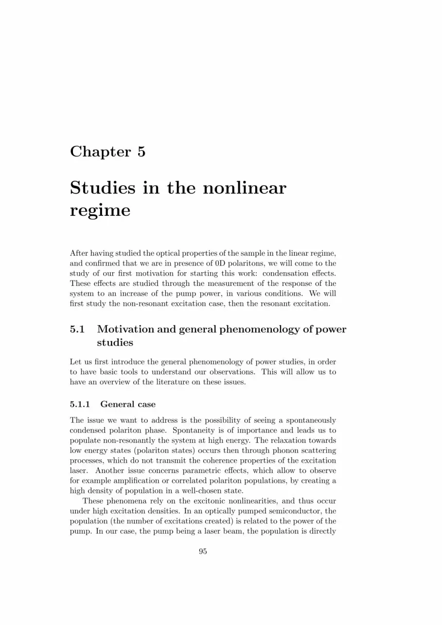
Chapter 5
Studies in the nonlinearregime
After having studied the optical properties of the sample in the linear regime,and confirmed that we are in presence of 0D polaritons, we will come to thestudy of our first motivation for starting this work: condensation effects.These effects are studied through the measurement of the response of thesystem to an increase of the pump power, in various conditions. We willfirst study the non-resonant excitation case, then the resonant excitation.
5.1 Motivation and general phenomenology of powerstudies
Let us first introduce the general phenomenology of power studies, in orderto have basic tools to understand our observations. This will allow us tohave an overview of the literature on these issues.
5.1.1 General case
The issue we want to address is the possibility of seeing a spontaneouslycondensed polariton phase. Spontaneity is of importance and leads us topopulate non-resonantly the system at high energy. The relaxation towardslow energy states (polariton states) occurs then through phonon scatteringprocesses, which do not transmit the coherence properties of the excitationlaser. Another issue concerns parametric effects, which allow to observefor example amplification or correlated polariton populations, by creating ahigh density of population in a well-chosen state.
These phenomena rely on the excitonic nonlinearities, and thus occurunder high excitation densities. In an optically pumped semiconductor, thepopulation (the number of excitations created) is related to the power of thepump. In our case, the pump being a laser beam, the population is directly
95

96 CHAPTER 5. STUDIES IN THE NONLINEAR REGIME
related to the power of this laser, depending on which sate is excited (itcan be a polariton state or a high energy state, creating unbound electron-hole pairs). The term population mean here population of total excitations(including free carriers, uncoupled -dark- excitons and polaritons).
So one can summarize as follows : we are performing a study of theresponse of the system to a variation of the pump power, which concretelymeans a study of a given state’s population (usually the ground state) asa function of the total population created (or the total number of ”excita-tions”).
A clear overview of the phenomenology of the nonlinear optical prop-erties of semiconductor systems (under a high excitation) can be found in[Klingshirn, 1995].
5.1.2 Case of polaritons
1. Non-resonant excitation
Polaritons are composite bosons, meaning that they can show stim-ulation effects, while they interact. This means that several regimes(linear and nonlinear) are expected while populating non-resonantlythe system at a high energy, see Fig.5.1 for an illustration. Each den-sity regime depends on the dominant mean of relaxation.
Energy
Non-resonant
excitation (Laser)
Studied level
Emitted Intensity = f(Laser Power): linear quadratic exponential (… linear )
Stimulation
phonons +collisions +stimulationDominant mean of relaxation:
Excitation power
Figure 5.1: Diagram of the various regimes that can be observed whilevarying the density of a quasi-bosonic system, in the case of a non-resonantexcitation.
Phonon relaxation In a very low density regime, the only relaxationprocess involves phonons, so relaxation rates do not depend ondensity, and the population of a given state (which energy is lower

5.1. MOTIVATION AND GENERAL PHENOMENOLOGY OF POWER STUDIES97
than the pump energy) will vary linearly with the pump power.It is an incoherent process. [Tassone et al., 1997]
Effect of Coulomb interaction Coulomb interaction enters into ac-count for excitons, yielding collisions between free carriers or highenergy excitons. If collisions are the dominant mean of relaxation,the relaxation rates depend on density, and a quadratic behaviorof the population as a function of the pump power is observed[Senellart et al., 2000].
Stimulation When, at a given energy level (most probably the groundlevel), the density of occupation exceeds 1 particle per state, thebosonic nature of the involved particles implies a stimulation ofthe transition by the population of the state. Meaning that thispopulation will depend exponentially on the pump power. [Porraset al., 2002]
Saturation At very high density, when the whole available amount ofpopulation created in the system is transfered to the stimulatedstate(s), or to a certain number of low-energy states (the stimu-lation regime may have not been reached), a linear evolution ofthe population as a function of the pump power reappears. It isindeed impossible to have more particles in the system than whatis created by the pump.
Weak coupling At high excitation densities, however not dependingon the regime, the strong exciton-photon coupling may be lost[Butte et al., 2002]. This will not affect the different regimes, thephenomenology described above is similar in strong and weakcoupling regimes, as it is driven by the excitons.
2. Resonant excitation
The term resonant excitation can be ambiguous, because one couldimagine exciting resonantly any electronic state of the system, whenusing this expression, we systematically mean ”resonant with a po-lariton state”, either 2D or 0D. In this case some differences can arisewith respect to the non-resonant case. The various regimes expectedare drawn on Fig.5.2.
The various density regimes still depend on the dominant mean ofrelaxation.
Phonon relaxation At very low densities, the only relaxation pro-cess involves phonons, exactly as in the precedent case.
Effect of Coulomb interaction The fermionic component of the ex-citons enter into account, yielding collisions between excitons to-wards a signal and an idler state. As mentioned in the theo-retical introduction, equation 1.15 yields a quadratic behavior of

98 CHAPTER 5. STUDIES IN THE NONLINEAR REGIME
Energy
Resonant excitation
(Laser)
Studied level
Stimulation
phonons +collisions +stimulationDominant mean of relaxation:
Excitation power
Emitted Intensity = f(Laser Power): linear quadratic exponential (… linear )
Figure 5.2: Diagram of the various regimes that can be observed whilevarying the density of a quasi-bosonic system. Non-resonant excitation.
the populated (signal and idler) states as a function of the ini-tial state population, and thus of the pump power. Usually thestudied state is a final state of the collision process. [Ciuti et al.,2001]
Stimulation When, in the final states of the collision process (usu-ally the studied state and its complementary with respect to thepumped state), the density of occupation exceeds 1 particle perstate, the bosonic character of the involved particles implies astimulation of the relaxation, and thus parametric oscillations[Savvidis et al., 2000, Stevenson et al., 2000, Ciuti et al., 2000].Meaning that this population will grow exponentially with thepump power.
Saturation At very high density, as in the non-resonant case, whenthe whole available amount of population created in the system istransfered to the stimulated states, a linear evolution of the pop-ulation as a function of the pump power reappears. A saturationof the absorption of the populated state is also possible.
Weak coupling At high densities the strong exciton-photon couplingmay be lost. As we are pumping in a polariton state, this willimply a loss of resonance between the pump and the pumpedstate, and may lead to optical bistability [Tredicucci et al., 1996].

5.2. NON-RESONANT EXCITATION 99
5.2 Non-resonant excitation
SpectroOptical filters
Microscope
objectiveSample
White light
Pellicule 4%
CCD with a 2D real space
image
•F=180mm or
•d’ conjugated to d for
reciprocal space imagingF=4.5mm
Cube
d
Optical axis
Lasers
Lens
Focal length 80mm
Figure 5.3: Set-up used to perform non-resonant excitation studies.
The set-up to pump non-resonantly the sample is shown on Fig.5.3,it allows to have energy dispersed images of one real or reciprocal spacedimension.
The sample was excited with different excitation conditions (laser energy,spot size), and at various detunings, we found no qualitative change in theresults depending on these parameters. Results in various conditions areshown.
5.2.1 Regimes observed
Let us study in details the case of the smallest mesas, where the modes arewell spectrally distinguishable. We will see several excitation conditions.
a - A 3µm mesa at zero detuning
The first example is a 3µm mesa at zero detuning for the ground confined po-lariton state, a photoluminescence spectrum in real space is shown on Fig.5.4(this spectrum was already shown and commented in chapter 4 Fig.4.5(a)).The mesa is excited with a continuous laser, showing a spot of ≈ 3µm at anenergy of 1.6eV (780nm, hence 0.12eV above the exciton energy), which cor-responds to the upper edge of the mirrors’ stopband. PL intensity, linewidth

100 CHAPTER 5. STUDIES IN THE NONLINEAR REGIME
En
erg
y (
meV
)
Position (µm)
Figure 5.4: PL intensity as a function of energy and position for a 3µm-diameter mesa. The same symbols than for the precedent chapters are usedto label the various states: grey circle for the 2D polaritons, black circle forthe confined ground state, white triangle for the confined first excited state,white rhombus for the confined second excited state.
and energy of the ground level of the confined LP are shown on Fig.5.5 as afunction of the laser power.
As we have mentioned before, the photoluminescence (PL) intensity is di-rectly related to the polariton population, through its photonic component.The first graph shown on Fig.5.5(a) is thus the angle and space-integratedPL intensity of the ground state (lowest energy level on Fig.5.4), in a Log-scale, as a function of the laser pump power. As one can see four regimesare clearly distinguishable: linear, quadratic, strongly nonlinear and linearagain. These regime fairly correspond to the phenomenology introduced atthe beginning of this chapter.
The question is now to determine what kind of particles we are address-ing. This means figuring out where the loss of the strong-coupling regimeoccurs. As this cross-over from strong to weak coupling is not a phase tran-sition, there is a wide density (or pump power) range where it is not clearwhether we are dealing with polaritons or not. Indeed the progressive exci-ton saturation diminishes progressively the oscillator strength and thus theRabi splitting. In order to determine the coupling regime, we have plotted

5.2. NON-RESONANT EXCITATION 101
two other types of data: energy and linewidth of the studied state. Twocriteria give lower and upper limits between which strong coupling is bro-ken1: one is the onset of the decrease of the linewidth, the other one is thecrossing between the PL peak and the uncoupled exciton line, these twoextreme criteria give a pump power range between 0.75 and 4mW for theloss of strong coupling. This ensures that the superlinear regime seen afterthe quadratic is in a state of weak coupling, it is the expression of laseroscillations (so we are in presence of an optically pumped VCSEL - VerticalCavity Surface Emitting Laser [Butte et al., 2002]), confirmed by the verysharp linewidth.
1See for more details section 1.4

102 CHAPTER 5. STUDIES IN THE NONLINEAR REGIME
103
104
105
106
107
108
109P
L in
tens
ity o
f the
0D
LP
gro
und
stat
e [a
rb. u
nits
]
121086420Pump Power [mW]
(a)
linear fit quadratic fit linear fit
2.0
1.5
1.0
0.5
0.0
Line
wid
th o
f the
0D
Low
er p
olar
iton
grou
nd s
tate
[meV
]
121086420Pump Power [mW]
(b)
1.4875
1.4870
1.4865
Ene
rgy
of th
e 0D
low
er p
olar
iton
(eV
)
121086420Pump Power [mW]
2D Exciton
(c)
Figure 5.5: (a) Photoluminescence intensity (semi-Log scale), (b) linewidthand (c) energy of the LP ground state of a 3µm mesa at zero detuning as afunction of the pump power. PL intensity was integrated angularly in orderto include all the emission of a given energy, corresponding to a given state,as we are in presence of a discrete spectrum.

5.2. NON-RESONANT EXCITATION 103
b - A 3µm mesa at negative detuning
We have performed the same kind of study in a different configuration: wechose a mesa where the ground photon level is at negative detuning withrespect to the exciton line energy (δ ≈ −7meV 2), and thus its excitoniccomponent is negligible. One would expect relaxation to be less efficient inthis configuration, and nonlinear thresholds to be higher.
The excitation is now done with a laser pumping at very high energy(2.43meV , it is a green Argon laser emitting at 512nm), with a spot ofabout 30µm in diameter.
Linear fit
Figure 5.6: PL intensity (semi-Log scale) and Linewidth of the ground levelof a 3µm mesa at negative detuning as a function of the pump power.
The behavior of the PL intensity, shown on Fig.5.6, is similar here to thebehavior observed at zero detuning, with two quantitative differences:
• An exponential behavior is clearly visible (it was barely visible onFig.5.5 between pump powers of 4.5 and 5mW .). This behavior is dueto a lasing in weak-coupling regime, we will see this further in section5.2.2.
2This means that the ground lower polariton state we are studying is at an energyequal to the uncoupled photon mode at the same position, strong coupling loss can thusnot be deduced from a an energy shift argument.

104 CHAPTER 5. STUDIES IN THE NONLINEAR REGIME
• The broadest linewidth reached is 100µeV (see Fig.5.6), to be com-pared to 2meV in the previous case ! This is the most visible effect ofthe difference in the excitonic components.
Occupation number We calculated the number of polaritons created inthe studied state at the quadratic threshold through a method inspired fromref. [Senellart et al., 2000]. As we integrate angularly the whole signal, wesimply measured the PL power emitted at the ground state energy at thethreshold, equal to approximately Pdetected ≈ 30nW . This power should bemultiplied by ' 2 in order to take into account the two sides of the cavity.
Nground state =Pdetectedτcav
C2E≈ 0.1polariton
where N is the number of polaritons in the state, τcav is the cavity photonlifetime, C is the Hopfield coefficient, and E is the energy of the state in Joule.The uncertainty is given by τcav = 10ps±5% and C2 can be considered equalto one (the error related to the error on the detuning which is around 5%)at such negative detuning. As one can see the uncertainty on this numberis around ≈ 10%, but nevertheless low enough to say that Nground state < 1.
Larger mesas
Identical studies were performed on larger mesas (9 and 19µm in diameter)and no qualitative difference was found.
5.2.2 Weak coupling regime
In order to check the onset of lasing in weak coupling regime on the wholesample, we performed in parallel 2 series of measurements along the sample’swedge, while pumping the mesas non-resonantly (with the same conditionsthan for the 3µm mesa at negative detuning), one well below the breaking ofthe strong coupling (in the linear regime) and one well above (in the lasingregime).
Each measurement is done exciting the system with a 30µm laser spot,far wider than the mesa, which means that both 0D and 2D signals areobservable. As we chose a position where the confined ground mode istuned around resonance with the exciton, the 2D cavity mode is positivelydetuned between δ ' +6meV and +8meV with respect to the exciton mode,thus the 2D-Lower polariton is exciton-like, this allows us to always havethe exciton signal on our spectrum, as a reference. At low excitation power,one sees on Fig.5.7 the usual anticrossing behavior between the 0D lowerpolariton and upper polariton (only the ground state is represented). Atvery high excitation power, only one mode can be seen, crossing the excitonline, it is the VCSEL lasing regime of the ground 0D cavity mode. One can

5.2. NON-RESONANT EXCITATION 105
note that this mode does not cross the exciton line precisely at the resonance(zero detuning) position. The latter is at a position x ' 10mm, where thesplitting between the 0D lower and upper polariton is the smallest. Thus,one can see that the energy of the lasing mode is slightly detuned towards lowenergies with respect to the uncoupled cavity mode. This may be attributedto the index refraction change at high excitation densities.
Stimulation in the weak coupling regime is characteristic of a VerticalCavity Surface Emitting Laser (VCSEL) [Butte et al., 2002], lasing is alsoconfirmed by the linewidths behavior on Fig.5.5(b) and Fig.5.6. This VCSELshows some peculiarities: it is optically pumped and lasing on a single mode(given by the 0D confinement). The single mode lasing could be of interestunder electrical injection [Hofmann et al., 2007], and the broad angularpattern of the ground mode indicates a behavior that recalls non-directionnallasing recently reported [van Vugt et al., 2006].
A beautiful succession of images3 on Fig.5.8 illustrates this progressiveloss of the strong-coupling regime, and then lasing on the ground photonmode. One can note on Figs.5.8(a) and (b) the intensity ”holes” in the 2Dupper and lower polariton signal we mentioned in chapter 4 section 4.1.4.
On Fig.5.8(e) the 0D uncoupled modes are clearly visible and severalconfined states are resolved. Finally on Fig.5.8(f) one can see the lasingregime on the ground confined photon state.
1.483
1.485
1.487
1.489
1.491
1.493
1.495
1.497
1.499
7.7 8.2 8.7 9.2 9.7 10.2 10.7
Position (mm)
En
ergy (
eV)
0D upper polariton 0D lower polariton 2D upper polariton
2D lower polariton 0D VCSEL laser
Figure 5.7: Anticrossing (at low pump power) and evolution of the VCSEL(high pump power) signal for the confined system. The 2D LP is at theexciton’s energy, as the 2D cavity shows strong positive detuning for thisrange of positions.
3Nicely designed and formatted by Gael Nardin.
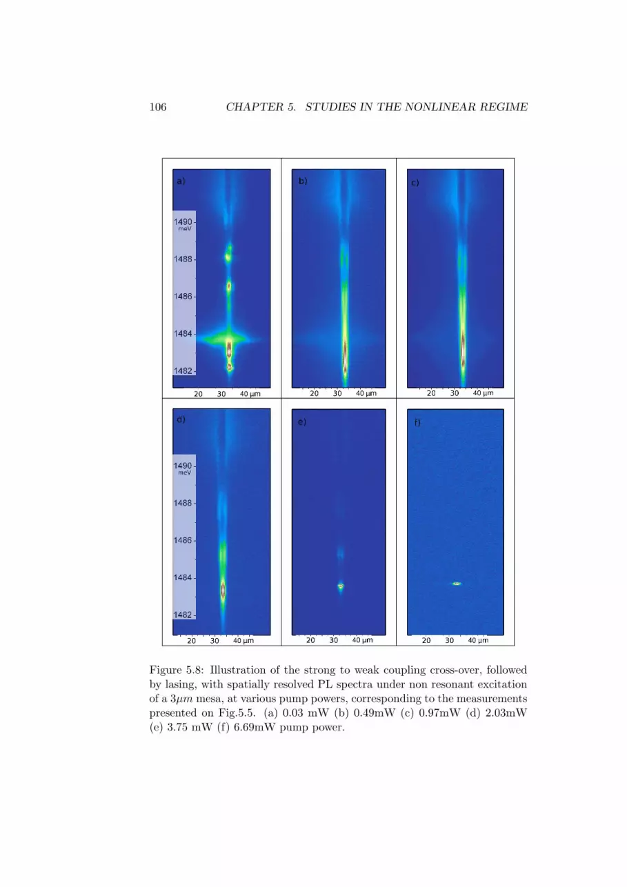
106 CHAPTER 5. STUDIES IN THE NONLINEAR REGIME
Figure 5.8: Illustration of the strong to weak coupling cross-over, followedby lasing, with spatially resolved PL spectra under non resonant excitationof a 3µm mesa, at various pump powers, corresponding to the measurementspresented on Fig.5.5. (a) 0.03 mW (b) 0.49mW (c) 0.97mW (d) 2.03mW(e) 3.75 mW (f) 6.69mW pump power.

5.2. NON-RESONANT EXCITATION 107
5.2.3 A lab for seeing nonlinear effects
We were able to observe successively and separately several kinds of be-haviors which can occur when increasing the density of quasi-bosons. Butthe nature of the studied particles changed during the study! Indeed thestimulation regime observed was in a situation of weak-coupling betweenexcitons and photons, this regime is representative of a photon condensedphase, a laser, where the active medium is the quantum well, and the cavitymodes are the confined mesa modes. The strong to weak-coupling regimetransition was observed through an increase of the excitation density, byexcitonic saturation and interaction. It is also possible to observe it througha variation of the temperature [Gutbrod et al., 1998].
Communicating vessels
An interesting point to mention is the comparative evolution of the confinedand 2D (or continuum) states. We could observe nonlinear behaviors onthe excited states of the mesa, similar to what was observed on the groundstate, although these behaviors appeared to be very unstable: the slightestperturbation in the experiment would drastically change the PL intensity,hence, it was not possible to draw their behavior on a large excitation powerrange. Moreover, in the same series of studies, we also observed nonlinearbehaviors of the 2D signal when increasing the pump, also accompanied bya strong-to-weak coupling regime transition.
Following these observations several interesting features should be men-tioned:
• The confined excited states show nonlinear thresholds similar to whatobserved for the ground level, at similar laser powers (though slightlyhigher). It is difficult to give precise values because of the instability ofthe system as soon as more than one state shows a nonlinear behavior.
• The 2D signal shows nonlinear behaviors at even higher thresholds(3-4 times higher). It shows a quadratic behavior, followed by anexponential in the weak coupling regime.
• When the 2D signal passes the transition from a quadratic to an expo-nential behavior, the 0D states show a change in their emission regimesimultaneously, but an opposite change, from what seems to be theonset of en exponential back to a quadratic regime. Fig.5.9 shows thisbehavior, it occurs in the weak coupling regime.
These measurements show that the 2D and 0D states share the samereservoir: when the 2D continuum states stimulate the relaxation towardsthem, the reservoir does not show sufficient population to allow the relax-ation stimulation towards the 0D states. The latter are then populated by

108 CHAPTER 5. STUDIES IN THE NONLINEAR REGIME
4.106
8.106
12.106
16.106
2.104
4.104
6.104
8.104
4.105
8.105
12.105
0
0
0
0D
gro
und s
tate
PL
inte
nsi
ty
0D
1st
exci
ted s
tate
PL
inte
nsi
ty
2D
PL
inte
nsi
ty
Figure 5.9: Upper graph: transition of the 2D signal towards a lasing regime.Lower two graphs: Falling of the mesa LP ground and first excited statesintensity, from a starting lasing regime (exponential) back to a quadraticregime. The quadratic fit was performed on the points taken before thetransition at 38mW . All scales are linear.
a process which stays present: Coulomb scattering in the pumped state (athigh energy).
In conclusion We observed a rich phenomenology of nonlinear effects.Moreover, spatial overlap of the 2D and 0D wave functions seems to besufficient to yield interaction. It is nevertheless difficult from this kind oftime-integrated measurement to obtain more information, and in particularto figure out if the 0D states populate each other. This would need time-resolved measurements of the population along one spatial axis, at givenenergies, in order to follow population and depopulation of the various states.This kind of measurements are being performed at the moment by TaofiqParaıso and Gael Nardin.

5.3. RESONANT EXCITATION: PARAMETRIC PROCESSES 109
5.3 Resonant excitation: parametric processes
The non-resonant excitation of the system creates free carriers contributingto the total density of population and thus to the strong-coupling loss. Res-onant excitation of the system creates only polaritons. It has lead to theobservation of several phenomena of interest as giant parametric amplifica-tion [Saba et al., 2001] or coherent control of polaritons [Kundermann et al.,2003] along with the varied phenomenology we introduced at the beginningof this chapter.
Resonant excitation concretely means excitation of the system througha polariton state. In order to excite selectively a given eigenstate, one needsto be able to observe these states. As they are defined in the wave vectors’basis, it is necessary to observe the reciprocal space of the sample in orderto be able to select which state to populate. As shown in chapter 4, thereciprocal space is accessible through angle resolved imaging and excitation.
5.3.1 Principles of parametric processes
We gave in section 5.1.2 the general phenomenology which can occur whileexciting resonantly a polariton system. Let us see more precisely the caseof the parametric oscillator. Since several years now parametric oscillations,a phenomenon similar to the optical parametric oscillator (OPO), was ob-served when pumping the system above a certain critical density: thanksto their excitonic content, polaritons can interact strongly, added to theirpeculiar dispersion shape, this allowed to observe polariton parametric scat-tering where two polaritons in a pump initial state (Ep, ~kp), scatters towardsone idler (Ei, ~ki) and one signal (Es, ~ks) states, along the LP dispersioncurve. These processes should respect energy and momentum conservation:2Ep = Es + Ei and 2 ~kp = ~ks + ~ki, see Fig.5.10.
Thanks to its non-parabolic shape, it is possible to find such states onthe lower dispersion branch, given that kp is larger than the inflection point[Langbein, 2004]. For one given pump state, the allowed couples of signalsand idlers are described by 8-shaped lines in the 2D reciprocal space, as wasobserved by Langbein [2004]. The most interesting pump state is at the so-called magic angle, for which the signal state corresponds to the bottom ofthe dispersion, that is the polariton ground state (E0,~k = ~0). This situationshows the smallest density threshold for parametric conversion [Savvidiset al., 2000, Stevenson et al., 2000, Ciuti et al., 2000], it is schematicallyshown on Fig.5.10.
As shown by Ciuti et al. [2001], the threshold for which parametric oscil-lations occur is the same than for the optical parametric oscillator (OPO).It is given by
∆kp,kp′ = √γ0γ2kp (5.1)

110 CHAPTER 5. STUDIES IN THE NONLINEAR REGIME
Idler
k
E
Pump
Signal
Figure 5.10: Diagram of the parametric scattering process when exciting atthe magic angle.
Where ∆kp,kp′ is the blueshift of the pump state, when this blueshift(due to the density increase) equals the linewidth because the scatteringrate equals the losses, the parametric oscillation starts. It is proportional tothe density of polaritons created in this state
∆kp,kp′ ∝ np (5.2)
SpectroOptical filters
Microscope
objectiveSample
White light
Pellicule 4%
CCD with a 2D real space
image
•F=180mm or
•d’ conjugated to d for
reciprocal space imagingF=4.5mm
Cube
d
Optical axis
Photograp
hic
objective
Lasers
Retroreflector:
Allows variation of
the excitation
angle
Figure 5.11: Set-up used to perform resonant excitation studies, the retro-reflector allows to change the angle of excitation both in the vertical andhorizontal dimensions, parallel to the cavity plane.
5.3.2 Setup
The set-up to pump resonantly the sample is shown on Fig.5.11, it allows tohave energy dispersed images of a dimension in real or reciprocal space, and
5.3. RESONANT EXCITATION: PARAMETRIC PROCESSES 111
to excite the system with a given angle. This means that we are creating apopulation of polaritons in a (nearly) single state, determined by the laser’senergy E and excitation angle.
The sample was excited with different excitation conditions (laser energy,spot size, continuous or pulsed), and at various detunings, but no qualitativechange was found to occur in the results depending on these parameters.
5.3.3 Parametric processes in the 2D cavity
Ep, kp
Ep, kp
Ei=2Ep, ki=2 kp
Es=0, ks=0
Ep, kp
Exchanged
quantity
(a)
1.486
1.490
1.494
1.482
En
erg
y (
eV)
Angle (°)
0-10 10
Figure 5.12: PL of the 2D polaritons in the reciprocal space: dispersioncurve. The pump laser energy and angle are indicated by a red disc.
In order to have an idea of the characteristics of this sample, comparedto other similar samples where parametric phenomena have been observed[Savvidis et al., 2000, Stevenson et al., 2000, Saba et al., 2001, Kundermannet al., 2003], we first performed a study of the 2D-polaritons’ behavior whenpumping resonantly at the so-called magic angle, as shown on Fig.5.12.
The excitation was chosen to be done with a pulsed laser, with pulselengths of 5ps, which means a linewidth of 1meV , this allows us to be inde-pendent from the blueshift of the polaritons (in particular the pumped state)dispersion curve with the increase of density. The dispersion is expected toshift energetically by the linewidth of the pumped polariton state ' 350µeVat the parametric oscillation threshold, small enough (< 0.5meV ) consider-ing the spectral linewidth of the laser. The laser spot size had a diameter

112 CHAPTER 5. STUDIES IN THE NONLINEAR REGIME
of ' 30µm and the sample was pumped at an angle of ' 8.
100x103
80
60
40
20
0
PL Inte
nsi
ty (
arb
.u.)
300250200150100500
Pump Power (µW)
Quadratic Fit
4
3
2
1
0
Energ
y s
hift
(% o
f th
e R
abi sp
litti
ng)
300250200150100500
Puissance laser
Linear fit
Figure 5.13: (a) PL Intensity of the bottom of the lower polariton dispersionas a function of the pump power. (b) Energy shift, the shift is by less thantwo linewidths, and keeps the energy far from the exciton line which is at1.487eV .
Results and interpretation
As seen on Fig.5.13, at low pump power, a linear behavior of the emissionpeak is observed, followed by a quadratic regime. After the latter, a linearregime appears, characteristic of the saturation in population of the system.
The quadratic behavior is due to a polariton polariton scattering belowthe parametric oscillation threshold, namely parametric luminescence, hav-ing the k = 0 state as the signal state. Fig.5.14 shows the evolution of the LPdispersion for various pump powers. Above the quadratic threshold, the sig-nal state is clearly dominant, but we were not able to observe the idler state.

5.3. RESONANT EXCITATION: PARAMETRIC PROCESSES 113
Pump Power 33µW 100µW 350µW
Ener
gy (
eV)
1.483
1.482
1.484
Angle (°)0 10-100 10-10 0 10-10
Figure 5.14: Evolution at various pump powers of the PL signal along theLP dispersion.
As it is at high wave vectors, its excitonic component is preponderant, sothe emitted intensity is weaker than for the k = 0 state. Another factor dueto this excitonic component is that it may relax by interaction with phononsand high k (non-radiative) excitons [Savona and Piermarocchi, 1997].
Nevertheless this state exists and certainly emits enough to be detectedwith a more sensitive apparatus as single-photon sensitive photodiodes. Cor-relation measurements could be made to show that photons emitted by thesignal ks and idler ki states are intensity-correlated (one photon is emittedin the idler state means that one photon is emitted simultaneously in thesignal state) [Karr et al., 2004]. But as no exponential behavior is observedbefore saturation, we can deduce the absence of stimulation and of para-metric oscillation, thus we do not expect any phase relation between signaland idler photons.
Threshold comparison
We saw in section 5.3.1 that the parametric oscillation density thresholddepends on the spectral linewidths of the polariton states. In order to try tofigure out why we did not observe any parametric scattering in this sample,let us compare the linewidths in various experiments: in the case of oursample (1.), the sample of Stevenson et al. [2000] (2.) and the sample ofKundermann et al. [2003] (3.). Let us assume that γ0 ' γkp ' γ2kp . Thelinewidths are:
1. ' 350µeV
2. ' 750µeV with three quantum wells and a Rabi splitting of ' 6meV
3. ' 100µeV with exactly the same structure and Rabi splitting thanours.
As we are not able to determine precisely the proportionality factor ofequation 5.2, we can assume that it is of the same order for similar structures,

114 CHAPTER 5. STUDIES IN THE NONLINEAR REGIME
but for the case (2.), as the number of quantum wells is multiplied by 3, theapparent saturation density is increased by a factor equal to this numberof quantum wells, as excitons in the various quantum wells do not interact,while the parametric oscillation threshold scales like the linewidth.
One can see that in case (2.) the threshold is twice higher than ours, butthe saturation density 3 times higher, so the threshold in term of excitationpower is twice lower. As for the case (3.), the threshold excitation powershould be in our case a little more than 3 times higher. These differencesare apparently significant enough to let a breaking of the strong-couplingappear before the parametric oscillation threshold, but after the parametricluminescence threshold.
5.3.4 Parametric processes in a 9µm mesa
En
erg
y (
eV)
1.482
1.483
(a) (b) (c)
Angle (°)0 1010
1.484
0 10100 1010
Non-resonantResonant
pump power 76µW
Resonant
pump power 280µW
Figure 5.15: (a) Dispersion in photoluminescence under non-resonant excita-tion of the 9µm-diameter mesa lower polariton at zero detuning, the whitesignal at high energy is the 2D lower polariton (at the exciton’s energy).The pump state and its potential signal below (respectively idler above) arecircled in red. (b) Resonant pumping with a spectrally broad laser. (c)Emission at the nonlinear threshold. Mentioned pump powers correspondto the experiment shown on Fig.5.16
We performed the same kind of experiment on 0D polaritons, in a firststep we will show the results for a 9µm-diameter mesa, as shown in theprecedent chapter, these mesas show a quantized quasi dispersion, the mesapresented in this section has a dispersion as shown on Fig.5.15(a). Theground state is at slightly negative detuning δ0D ' −0.25meV .
The excitation conditions are as described for the 2D-polaritons, theenergy linewidth of the pump laser allows here again to be independentfrom the possible shift of the pumped levels, as can be seen on Fig.5.15(b),the excitation angle is ' 10, and the central energy of the laser pulse is1483.3meV . One can see on the reciprocal space images (taken in PL whilepumping non-resonantly) that the confined states have lobes depending on

5.3. RESONANT EXCITATION: PARAMETRIC PROCESSES 115
0.20
0.18
0.16
0.14
0.12
0.10
0.08
0.06
Line
wid
th (
meV
)
4003002001000Laser Power (µW)
First excited level Ground level
1.48560
1.48555
1.48550
1.48545
1.48540
1.48535
1.48530
Peak
ene
rgy
(meV
)
4003002001000Laser power (µW)
First excited level Ground level
600x103
500
400
300
200
100
0
PL In
tens
ity o
f th
e 0D
gro
und
leve
l (ar
b.u.
)
4003002001000Laser Power (µW)
Quadratic fitLinear fit
(a)
(b)
(c)
0.08Rabi
0.02Rabi
Figure 5.16: (a) PL intensity of the lower polariton ground confined level asa function of the laser power. (b) Linewidth of the lower polariton groundconfined level (red squares), and first excited level (blue squares). (c) Energyshift of the lower polariton ground confined level (red squares), and firstexcited level (blue squares), the ratio of the largest shift over the Rabisplitting is given.

116 CHAPTER 5. STUDIES IN THE NONLINEAR REGIME
the angle of detection4, so at the angle which was chosen to populate thesystem shown on Fig.5.15, corresponds to a lobe. The energy chosen shows asignal-idler couple of states fulfilling the energy conservation with a precisionbetter than the linewidth: Eidler−Epump = 0.87meV and Epump−Esignal =0.90meV , where the signal state is the LP ground confined state. Thesevalues are smaller than the linewidth of the confined photon: 0.90− 0.87 =0.03meV < 0.1meV ' γ0D, and thus of the confined polariton.
Results
Results obtained are shown on Fig.5.16, as in the 2D case, three regimes aredistinguishable: linear, quadratic and linear again. We integrated the wholeangular extension of the 0D ground state, the signal shown on Fig.5.16(a) isthus directly proportional to the whole population of this state. A quadraticfit describes well the evolution between 60 and 260µW . We were easily ableto trace the evolution of the linewidth and energy of this state on Fig.5.16(b)and (c), there is indeed a small increase of the linewidth due to densityeffects. There is also for the same reason a slight blueshift of the resonanceenergy.
The quadratic regime can be attributed to parametric luminescence (po-lariton polariton scattering), as in the precedent case, the following linearregime can be attributed to a saturation in population, it may also be due toa loss of the strong-coupling regime, but as there is no significant blueshift,it is not possible to conclude with certainty. We will discuss further thisissue at the end of this chapter.
5.3.5 Continuous wave pumping of a 9µm mesa
0.065*!R
Figure 5.17: PL intensity (a) and energy (b) of the LP ground mode of a9µm mesa, as a function of the pump power, under continuous wave resonantpumping.
4These lobes correspond to the quantum number m.

5.3. RESONANT EXCITATION: PARAMETRIC PROCESSES 117
For sake of comparison, we performed the same kind of experiment un-der resonant continuous pumping, tuning the laser’s energy at every pumppower, in order to keep it resonant with the blueshifted pumped polaritonstate. As seen on Fig.5.17, we observed similar behaviors than in pulsedpumping, with 3 successive regimes: linear, quadratic and then linear again,and a very small shift of the resonance.
Thresholds
The nonlinear threshold appears at a pump density of 150W/cm2. Thisthreshold value allows us to calculate the number of polaritons created inthe pump state through a method inspired from ref. [Senellart et al., 2000].The first step is to calculate, from the pump density above, which poweris reaching the mesa, with its 9µm in diameter, from a 40µm spot. Thesecond step is, in reciprocal space, to take into account the fact that weare not in presence of a continuous dispersion curve. As one can see onFig.5.15, the pumped state (fourth energy level, starting from the lowest)has a certain angular width. We saw in chapter 4 that at a given energy,the degeneracy can not be easily evaluated. We will therefore consider thatthe quantized character of the energy dependence ensures us that we arepopulating one state having a ring angular profile. Nevertheless the state isnot homogeneously excited on all its angular extension. The laser excites alocalized zone within this ring, we calculated this zone to represent around11.5% of this zone in surface. This yields the following expression:
Npump =Plaserτcav
C2E∗ 11.5/100 ≈ 1000polaritons
where N is the number of polaritons in the state, Plaser is the laser powerimpinging on the mesa surface in Watt, τcav is the cavity photon lifetime,C is the Hopfield coefficient and E is the energy of the state in Joule. Withτcav = 10ps±5% and C2 = 1/2±20%. One should also to take into accounta coupling factor between the external laser field and the cavity internalelectromagnetic field, this factor could diminish the effective laser power ofone order of magnitude.
The final deduction reads then 50 < N < 1500 polaritons. Thus
Npolaritons in the pumped state >> 1
This number should imply a saturation or nonlinear behaviors, we will seethat several interpretations are possible for the pumped state behavior insection 5.3.7.
Excited states behavior
Thanks to the quantized character of the system, we were also able to studythe behavior of the first excited state of the 0D lower polariton. During the

118 CHAPTER 5. STUDIES IN THE NONLINEAR REGIME
fast quadratic increase of the ground state’s intensity, it becomes impossibleto distinguish the first excited state from the side of the ground state. It isnevertheless clear that both studied state show a blueshift. As the density ofpolariton per state did in principle not go beyond one (otherwise we wouldhave observed a stimulation effect), the blueshift shows that the confinedlevel are sensitive to the overall density of polariton in the mesa.
(a) (b)
2006juin2
En
erg
y (
eV)
1.483
1.482
1.484
Angle (°)0 10-10
0 10-10
Angle (°)0 10-10
Figure 5.18: Continuous wave resonant pumping of a 9µm mesa at1.48645eV , corresponding to the horizontal line on both figures, but at anangle not contained in the k−dimension shown. (a) Linear relaxation regime,the whole lower polariton curve below the pumping energy is visible. (b)Both the ground and first excited states are in a quadratic regime.
This explains the change of regime for excited states of the mesa whichwe observed, although we could not plot the PL intensity as a function of thepump laser power for these excited states, because they showed high fluctu-ations and instabilities. It was nevertheless possible to take two interestingimages of the dispersion curve, which can be seen on Fig.5.18(a) and (b).Fig.5.18(b) shows a situation where both the ground and first excited statesare in a quadratic regime, this is why the first excited state’s luminescencecan be seen and is not hidden by the ground state’s luminescence.
This situation is consistent with the observations reported in section 5.2.3where, as the system is non-resonantly pumped, the ground LP confined leveland the first excited level show several regimes.
5.3.6 Resonant excitation of a 3µm mesa at zero detuning
Similar studies were performed on the 3µm mesa studied in chapter 4, itsspectrum is shown on Fig.4.5(a). In the case shown here the excitation laserwas a continuous wave laser, the excitation was done in reflection. As thereare only three 0D confined lower polariton levels, we simply chose to excitethe middle one (so the first excited level), with a broad angular aperture of30.
The energy difference between the pumped mode (first excited) andthe ground mode (respectively the second excited) is 0.79meV (respectively

5.3. RESONANT EXCITATION: PARAMETRIC PROCESSES 119
0.89meV ). The energy matching is fulfilled with a precision approximatelytwice smaller than the polariton linewidth. We did not do any angular se-lection in the excitation, as there is a wide k−space delocalisation of theenergy. The resulting behavior is shown on Fig.5.19, it is qualitatively sim-ilar to what was observed for the ground state of the 9µm mesa studiedabove.
50x103
40
30
20
10
0PL inte
nsity o
f th
e 0
D L
P g
round s
tate
[arb
units]
1400120010008006004002000
Pump Power [!W]
Quadratic fit Linear fit
Figure 5.19: PL intensity of the lower polariton ground confined level as afunction of the laser power. A quadratic and a linear fit are shown.

120 CHAPTER 5. STUDIES IN THE NONLINEAR REGIME
5.3.7 Alternative points of view: signs of bistability?
One can see that the behavior of the ground state of the system as a functionof the pump power is fairly reproducible in the mesas, as can be seen onFigs. 5.19, 5.17 and 5.16. It consists of a linear behavior followed by aquadratic one, and then linear again. Although we gave an explanation tothe various regimes we observed, we did not expect to see a linear regimebefore any parametric oscillation behavior.
The fundamental reason may be related to the phase and energy-matchingconditions required to observe parametric conversion behaviors. We sawthat energy-matching conditions were always fairly fulfilled, but in a con-fined quantized level a small mismatch is unavoidable. One possibility, totry to improve these conditions fulfillment, is to tune temperature, but thestrong-coupling regime can not be guarantied any more after 30K becauseof the broadening of the exciton resonance. Rapid power studies at tem-peratures till 30K did not show any qualitatively different behavior. Onthe other hand, phase-matching conditions consist here in conditions on theconservation of the azimuthal m quantum number. It is however difficult todetermine with certainty whether these conditions are fulfilled or not. Wesaw in chapter 4 that we probably excite a superposition of modes, and canonly suppose (and hope!) that the suitable quantum number combinationis excited through this superposition.
We tried to adopt another point of view for the description of the collisionphenomena observed: we were able to fit the peculiar shapes of the groundstate intensity evolution by cubic polynomial expressions, by inverting thetwo axes of the plotted graphs. Fig.5.20 shows again the evolution of theemitted PL intensity of the ground state for a 9µm mesa in two cases studiedin this chapter, but with another point of view: the pump power is plottedas a function of the emitted PL intensity. A cubic fit was done and fits verywell the measurements.
20
15
10
5
0
Las
er p
ow
er (
mW
)
1.5x10⁶
1.00.50.0
Ground state PL (arb.u.)
400
300
200
100
0
Las
er p
ow
er (!
W)
600x103
5004003002001000
Ground state PL (arb.u.)
(a) (b)
Figure 5.20: Cubic fit of the pump power as a function of the ground statePL intensity for the case of (a)Fig. 5.16 and (b) 5.17. The fits are performedon the whole range of points taken.

5.3. RESONANT EXCITATION: PARAMETRIC PROCESSES 121
This dependence is characteristic of bistable phenomena: for a givenvalue of one of the fit parameters, a cubic dependence can show a hysteresiscycle, characteristic of bistable phenomena. Two different phenomena canbe concerned here:
Degenerate scattering
This dependence can be characteristic of a degenerate parametric oscillator,meaning that the polaritons scatter within a single state. The population ofthe considered state evolves in this case as follows, as demonstrated througha mean-field theory by A. Baas and his colleagues in ref. [Baas et al., 2004],and as detailed in his thesis [Baas, 2003]:
np(γ2p + (δp + αpnp)2) = 2γmC2
0Iin (5.3)
Where np is the mean number of polaritons in the considered state,γp = C2
0γC+X20γX is the linewidth of the polariton branch, δp is the detuning
of the laser with respect to the pumped polariton energy, and γm is thedissipation coefficient coefficient of the mirror through which the system isbeing pumped, this coefficient needs to be taken into account as the laseris not necessarily resonant. For certain values of δp, equation 5.3 shows ahysteresis characteristic of a bistability behavior which was observed in thereferences mentioned ([Baas et al., 2004] and [Baas, 2003]) of the emittedPL intensity versus the pump power (i.e. the mean number of polaritonsnp).
We tried to perform new series of measurements varying exclusively oneparameter: the pump power of a continuous wave laser. This experimentis similar to the one shown in section 5.3.5 but we did not tune the laser’senergy or any other parameter, trying to fix the parameter δp. The resultof this experiment is shown on Fig.5.21 in two configurations: on the firstgraph we performed the usual quadratic and linear fits, on the second graphwe draw, as opposed to usual, the pump power as a function of the groundlevel population, this shows a clear cubic dependence. However, we did notobserve any hysteresis or instability behavior. The variation of the variousparameters were always smooth. We tried to impose δp > 0, a situationwhich should show hysteresis, but were never able to observe any hysteresisnor to find the corresponding value in the fitting parameters.
This interpretation would mean that polaritons scatter coherently withinthe pumped state (where energy and phase-matching conditions are obvi-ously fulfilled) yielding a nonlinear dependence of the polariton field withIin. Polaritons then relax linearly through phonons towards the groundstate. The evolution of the ground state population is thus representativeof the evolution of the pumped state population.
This point of view suggests that we are in presence of a degenerateparametric oscillator in the pumped state. But this phenomenon, for positive

122 CHAPTER 5. STUDIES IN THE NONLINEAR REGIME
Quadratic fit
Linear fit
Cubic fit
(a)
(b)
Figure 5.21: Evolution of the ground state PL intensity of a 9µm mesa, seenin two different ways: on one graph the PL intensity is shown as a functionof the pump power, in the other graph it is the pump power which is seenas a function of the PL intensity.
values of δp, detuning of the laser energy with respect to the pumped stateenergy, should show a bistable behavior. However, despite several differentvalues of δp tried, we were not able to observe any bistability. Added tothat, we did not manage to fit in the same way the data taken for otherkinds of mesas, or for the 2D polaritons, neither to take new data whichwould show the same behavior. We will hence try to adopt again a differentpoint of view.
Bleaching of the strong-coupling regime
Tredicucci et al. [1996] suggests another phenomena yielding a bistable be-havior in the dependence of a polariton population with respect to a pump

5.4. BALANCE AND CONCLUSIONS 123
intensity: the bleaching of the strong coupling regime, while exciting reso-nantly a polariton state. The developed model uses the experimental pa-rameters of Norris et al. [1995] (an AlGaAs/AlAs cavity with five embeddedGaAs quantum wells). This may explain the apparent absence of loss ofstrong-coupling, despite the high pump powers reached: the system reachesan equilibrium between
• a blueshift of the LP resonance (due to the strong-coupling bleaching)decreasing the coupling efficiency between the laser and the polaritonresonance
• a redshift of the resonance back to the LP energy, when the laseris not efficiently coulped anymore, and thus does not create a highpopulation density in the system
These two phenomena of course reach an equilibrium corresponding tothe cubic dependence we observed. According to Tredicucci et al., bistabil-ity depends on a broadening factor directly related to the linewidth of theexciton resonance. If the latter is too large, no bistability is observed, butsimply a cubic behavior. We could therefore not tune this parameter, as weworked on one sample showing a given linewidth.
Future samples with various exciton linewidths may help us to discrim-inate between the various possible phenomena which one we observed.
5.4 Balance and conclusions
We performed many different studies, sharing all a same objective: the ob-servation of a massive redistribution of the polariton population towards asingle state. A phenomenon which would lead us towards condensation inthe case of non-resonant pumping, and which would open the way to para-metric oscillation and amplification in the case of a resonant pumping. Wedid not observe any of these phenomena, most probably because the non-linear thresholds were too high, compared to the strong-to-weak couplingthreshold. A solution to overcome this effect would be to increase the num-ber of quantum wells within the cavity, as we will see in chapter 7. Thiscould yield an increase of the strong-to-weak-coupling transition withoutaffecting the nonlinear threshold.
5.4.1 Balance of the observed phenomena
Let us recall and classify the diverse and rich phenomenology
1. Non-resonant excitation:
Phonons and collisions In any configuration we tried (size of themesa or detuning), we observed a relaxation towards the ground

124 CHAPTER 5. STUDIES IN THE NONLINEAR REGIME
state of the system through phonons at low densities and thencollisions, characterized by a quadratic dependence of the PL withrespect to the pump power.
Loss of the strong-coupling regime During the quadratic regime,we systematically observe a loss of the strong-coupling regime.
VCSEL This loss of strong-coupling is followed by a lasing regimecharacteristic of VCSEL.
2. Resonant excitation:
Nonlinearities We observed nonlinear behaviors (a quadratic increaseof the PL as a function of the pump) of the confined lower po-lariton, for any size of confinement.
Saturation This nonlinearity is followed by a linear behavior in thecase of 3 and 9µm mesas.
Bistability? We were able to fit the behavior of the pumped state ofthe 9µ mesa with a cubic fit. This kind of dependence can showhysteresis for certain values of the fitting parameter. This hys-teresis is a sign of optical bistability, either through a process ofdegenerate scattering in the pumped state, either through bleach-ing of the strong-coupling regime and loss of resonance with thelaser. We did not observe this, probably because of the impossi-bility to play on the suitable fitting parameter.
3. Interactions
Trapping mechanism We nevertheless could improve the understand-ing of the trapping mechanism: our observations of sections 5.2.3indeed tend to prove that the 2D and 0D polaritons share thesame reservoir.
Effective density We confirmed in section 5.3.5 that the confinedlevels are sensitive to the overall density of polaritons, althoughthey do not necessarily feel the same effective density, dependingon spatial overlaps of the wave functions.
5.4.2 Conclusion
It is the first time that these nonlinear phenomena are observed with con-fined 0D polaritons in a doubtless strong-coupling regime. In the precedentcases, it was not possible to observe directly the strong-coupling regime:either due to the temperature increase [Bajoni et al., 2007], yielding an in-crease of the linewidths; or due to the impossibility to measure the upperpolariton [Dasbach et al., 2001].

5.4. BALANCE AND CONCLUSIONS 125
The observations under resonant non-excitation are now well understood:the interplay between zero and two dimensional polaritons is promising forfurther relaxation studies.
Further studies would need to be done in order to discriminate betweenthe various interpretations we propose. Whatever the right interpretationproves to be, we already have clearly proven the occurence of nonlinearphenomena, and the potentiality to observe bistability phenomena.
This varied phenomenology is promising under resonant excitation bothfor applied (Fast switching using microcavities [Tredicucci et al., 1996], singlephoton emitters see [Deveaud-Pledran et al., 2006] and references therein)and fundamental (Study of optical bistabilities, of photon and polaritonblockade, of ultralow threshold lasers [Baas et al., 2004, Imamoglu et al.,1996, Verger et al., 2006]) physics.

126 CHAPTER 5. STUDIES IN THE NONLINEAR REGIME

Part III
Perspectives and discussions
127


Chapter 6
Applications
We propose in this section some potential applications based on the structureintroduced and developed in this thesis, we will discuss their feasibility anduse.
Based on this work, two patents were deposited, the first one about apolariton single photon source [Deveaud-Pledran et al., 2006], which theoret-ical description was developed in a paper by Verger et al. (C. Ciuti, coauthorof this paper, is coauthor of the patent), the second about a polariton twinphoton source [Daıf et al., 2006a], based on the idea of parametric scatteringin a confined polariton system1.
We will first describe rapidly the principles of these two patents, as theymay be potential starting points to applications based on the structure de-scribed in this work. We will then discuss their feasibility and more ingeneral the proximity of applications based on microcavity polaritons, ac-cording to the state of the art described all along this work, and in thereferences we could reach.
6.1 Polariton single photon source
Single photon sources are potentially important devices for quantum com-munications. Presently, the realization of single photon sources is based onthe attenuation of a laser beam, down to the level where the photons may bestatistically separated with a good probability. A wide range of improvedsingle photon sources has been proposed, mostly based on the use of theemission of a single quantum dot. The prominent publications in this fieldbeing the realization of an electrically driven single photon source [Yuanet al., 2002, Park et al., 2004]. Such sources offer the strong advantage ofcompactness, with the drawback of poor collection efficiency and a repeti-tion rate limited by the lifetime of the carrier pairs in the dot to about 100
1For more details the reader can refer to ref. [Verger et al., 2006] and references therein,and we recall that chapter 5 deals with issue.
129

130 CHAPTER 6. APPLICATIONS
MHz.
A device based on 0D polaritons could constitute a very efficient singlephoton source with a very high repetition rate. The collection efficiency mayin principle be made very close to 100% by proper tailoring of the parametersof the device, and the repetition rate may be improved by at least a factorof 100 to reach 10 GHz.
6.1.1 Principle
Given a 0D polariton trap as presented in this work, simple calculationsbased on the exciton nonlinear interactions show that when two polaritonsare present in the trap, the renormalized single-polariton energy is blueshifted by an amount comparable or even larger than its linewidth, pro-vided that the trap size is smaller than a critical value [Imamoglu et al.,1996, Verger et al., 2006]. For typical GaAs-like parameters, a blue shift ofthe order of 100µeV is computed for a trap lateral size of the order of onemicron [Verger et al., 2006]. Hence, the dynamics of a polariton trap witha size around or below 1 micron becomes strongly nonlinear already at thesingle polariton level, which explains in simple terms why the light emissionout of the polariton traps can be highly non-classical. In fact, the absorp-tion of a nearly resonant laser beam, with a frequency slightly red shiftedwith respect to the polariton ground mode (or resonant with it) is quantumblocked when the excited number of trapped polaritons exceeds one. Thisis analog to the photon blockade effect predicted for optical cavities con-taining atoms [Imamoglu et al., 1996]. The experimental set-up necessaryto produce such signal is sketched on Fig.6.1. In order to demonstrate thesingle photon nature of the emitted signal, one should add a second-ordercorrelation measurement set-up at the detection.
Laser
Spectral filter
Collecting lens
Detectors
Figure 6.1: Principle of the experimental set-up to be used to create single-photons on-demand.

6.2. TWIN PHOTON SOURCE IN THE NEAR INFRARED 131
6.1.2 Potential advantages
If the pump intensity is low enough, only one polariton can be excited in thepolariton trap. The polariton will then escape the trap within the radiativetime (around 10 ps) before another polariton can be re-injected inside thetrap. Excitation by a pulsed laser with a spectral width comparable orsmaller than the polariton linewidth will lead to the emission of single-photon pulses on demand out of the polariton traps. The repetition period,being limited only by the pulse duration, will be of the order of a few tens ofpicoseconds, i.e. a repetition rate more than 2 orders of magnitude higherthan in electronic quantum dot single-photon emitters. Moreover, unlikeself-assembled electronic quantum dots, the spatial position of polaritontraps can be fully controlled by the lithography (see chapter 2), paving theway to the realization of integrated arrays of single-photon emitters whoseexcitation and detection can be efficiently obtained through the use of opticalfibers.
6.2 Twin photon source in the near infrared
6.2.1 Existing devices and principle
A twin photon source presents two optical outputs in which the photons arestrongly correlated. If one photon is emitted through one of the two outputs,there is necessarily one corresponding photon at the other output. This typeof source is very interesting from a fundamental point of view, as it is basedon one of the main concepts of quantum mechanics: entanglement. From anapplied point of view, it is for example often used in quantum cryptographyexperiments or in quantum information protocols.
The twin sources usually used are optical parametric oscillators (OPO),which present very strong quantum correlations between the photons ofthe two outputs. They use parametric scattering to produce the quantumcorrelated emission.
A similar device was developed using parametric oscillation with a verylow pump intensity threshold, in a similar but original structure, thoughnot based on strong coupling: a triple cavity with embedded quantum wells[Diederichs and Tignon, 2005]. The peculiar shape of the dispersion of thetriple cavity allows to observe the pump, signal and idler states with similarintensities [Diederichs et al., 2006].
6.2.2 Feasibility with 0D polaritons: use of polariton para-metric scattering
The demonstration of polariton parametric oscillation in semiconductors hasbeen followed by many proposals for the measurement of quantum correla-tions between signal and idler modes. But they all come up against the same

132 CHAPTER 6. APPLICATIONS
problem, which is that signal and idler polariton modes have very differentphotonic components. This yields signal and idler radiative emissions thatare strongly detuned in intensity. In our case the signal and idler modes willhave similar photonic components, with a precision better than a few per-cents, the corresponding emissions thus will have almost the same intensity.A polariton trap can present a lot of discrete levels, therefore offering in thesame sample several sets of three levels for the parametric oscillation. Oncethe set chosen, the energy splitting between the three levels can be tuned inthe same sample, simply by changing the position of the excitation spot onthe sample in order to modify the exciton-cavity detuning.
The semiconductor device would present several advantages compared toan OPO: The structure is monolithic, the cavity doesn’t need to be alignedand the cavity thickness doesn’t need to be electronically controlled.
6.2.3 Advantages of 0D polaritons
It is possible to realize this in a semiconductor microcavity in strong couplingregime similar to the sample presented in this work. These zero dimensionalpolaritons can show several accessible levels, which positions depend onthe lateral size and depth of the trap. As we saw in chapter 2, a suitablecalibration allows to conceive a trap with precise depth and width. Westudied in chapters 3 and 4, the relation between the dimensions of thetraps and the number and spectral profile (in real and reciprocal spaces) ofthe confined states. We are now able to design a sample where three levelsare positioned in such a way that one is equally spectrally separated fromthe two others. This level will be the pump mode, and the two others thesignal and idler modes, for the parametric oscillation.
The experiment can be done in the continuous wave regime, producing inthis case quantum correlated beams, which entanglement can be evidencedby noise measurements [Karr et al., 2004] on the beam. This configurationcould be useful for protocols of quantum information with continuous vari-ables. It can also work in pulsed regime and produce few signal-idler pairsper pulse. As the polariton modes have the same photonic component, thesignal and idler emission have the same intensity and can be both attenu-ated in the same way without losing the correlation in order to have singlepairs.
Two different configurations have to be considered, depending on thepolarization of the pump. For a circularly polarized pump, the parametriceffect, that conserves the spin, will produce signal and idler pairs polarizedas the pump. This yields entanglement in intensity. For a linearly polarizedpump, signal and idler pairs will be totally unpolarized and the entanglementwill be in polarization. It can be detected as represented on Fig.6.22.
2Courtesy of Augustin Baas.

6.3. FEASIBILITY 133Twin photon source in the near infrared
3
Fig 2. Scheme of the experiment of entanglement in polarization. Two different configurations have to be considered, depending on the polarization of the pump. For a circularly polarized pump, the parametric effect, that conserves the spin, will produce signal and idler pairs polarized as the pump. This yields entanglement in intensity. For a linearly polarized pump, signal and idler pairs will be totally unpolarized and the entanglement will be in polarization. It can be detected as represented on Fig. 2.
Figure 6.2: Principle of the twin photon source.
This idea of using confined polaritons having similar photonic compo-nents is the basis of ref. [Bajoni et al., 2007] we mentioned in chapter 5.3.
6.3 Feasibility
At the moment, given the experimental conditions under which the presentedstructures show the suitable properties, it is not realistic to think aboutindustrial applications for the two ideas developed above. Nevertheless, therealization of these devices at low operating temperatures is feasible in thenear future. As we will see in the next chapter, it depends strongly onthe reliability of the samples’ source (so the MBE). As one understandsintuitively, a reliable source of samples is necessary in order to fabricateoriginal structures. This aspect is being worked on by Francois Morier-Genoud, Gael Nardin, and Taofiq Paraıso.
These devices could be used for various kinds of research, as a reliablesingle photon or correlated photon source. The latter is indeed needed forquantum communication and cryptography experiments, as well as a reliablecorrelated photon source3.
This potential opening is a concrete application for these proposals, asit is for the structure developed by Diederichs et al. [2006]. We wouldtend to propose that, as the mentioned researches are so far performed inan overwhelming majority by public laboratories, the application can not becalled industrial. This kind of knowledge is being published in open scientificjournals, and these proposals could also be published, in a near future, asan ensemble of useful proposals for experimentalists.
3The interested reader can have a look at the work performed in the group of appliedoptics (GAP) of the University of Geneva, cf. http://www.unige.ch/gap/welcome.html

134 CHAPTER 6. APPLICATIONS
6.3.1 Global warming!
Are industrial applications based on polaritons, and further on polaritonBEC, realistic? Several steps are now further needed for thinking aboutindustrial applications: the ease of high-quality sample production, and theon-demand production of room temperature strong-coupling under electricalinjection, followed by room-temperature BEC.
The strong-coupling at room temperature seems to be now establishedin nitride based materials [Christmann et al., 2006], although the ratio Ω/γ(which is an indicator of the coupling strength) needs to be improved. Sev-eral groups are working on strong-coupling under electrical injection. A veryrecent paper [Hofmann et al., 2007] reports the observation of a suitable exci-tonic emission in an InGaAs quantum well, that should allow strong-couplingto be observed under electrical injection for the first time.
Finally BEC was observed, but within a sample which is in principlereproducible, as the parameters of its growth were carefully chosen, butwhich at the moment no group is able to reproduce.
The convergence of these various parameters (quality, room-remperature,electrical injection, ease...) is necessary in order to think about furtherapplications. So industrial considerations are not surrealistic, it is simply abit early.

Chapter 7
Experimental perspectives
Now that we have discussed long-term perspectives, let us finish this workby discussing short term perspectives that our successors are already leadingor that could be the near future.
We will first have a look at what could be done on the present sample,in order to further understand relaxation mechanisms towards the trappedstates. We will then see how we could fabricate a new sample, through dif-ferent techniques. We will then see what interesting experiments could bedone with condensed phases, obtained either through spontaneous conden-sation or through parametric scattering. Indeed we designed a new mask,with new trap shapes, which could allow a wide variety of experiments inthe condensed regime, but also with a non-condensed fluid of polaritons.
7.1 Perspectives on this sample
We present in this work the achievement of a polariton trapping structure,on which we performed a large number of time-integrated studies. Severalaxes can be taken for the future work on this first achieved sample. Thefirst and most original one, compared to what was done so far, is to adda time-resolution to the set-up1, another interesting axis would be to tryto complete the imaging experiments presented in chapter 4, and finally tounderstand definitely the nonlinear behaviors observed in chapter 5, section5.3.
1Taofiq Paraıso and Gael Nardin (who are taking over with the confined polaritonsproject) and Sebastien Beaumont (who did a diploma work –master’s- with us), are per-forming, among others, time-resolved experiments.
135

136 CHAPTER 7. EXPERIMENTAL PERSPECTIVES
7.1.1 Time-resolved studies
Spectrally and time-resolved studies
First time-resolved images were already taken with spectral filtering. We willnot enter into the details of the set-up and of the streak-camera principle, themost important for us is to know what kind of images were taken: the streak-camera is placed after the spectrometer, takes from the latter a spectrallydispersed image of a real space line (E, x) and, disperses energy in time ata given position, usually chosen to be the center of a mesa. One can see theprinciple2 applied to a 9µm mesa on Fig.7.1.
1.482
1.484
1.486
1.488
En
erg
y (
eV)
1.482
1.484
En
erg
y (
eV)
0 400 800 1200 1600Time (ps)Position (µm)
0 10-10 2000
Figure 7.1: Principle of the streak camera applied to a 0D polariton signal:time dispersion of one band at a given position of the (E, x) space.
The preliminary results tend to confirm the interaction between 2D and0D polaritons, through different relaxation times. They also clearly showseveral relaxation times depending on the relaxation mean: through polari-ton scattering or phonons.
Next step: spectrally and spatially resolved time-resolved studies
In order to deepen the study, it will be interesting to see, at a given energy,the behavior along a whole spatial line. Figure 7.2 shows an example ofa line which could be selected and then dispersed in time. One could se-lect successively lines at relevant energies, including the 2D lower polaritonenergy, and reconstruct a 3D image (E, x, t).
Some work about the propagation of polaritons was performed by Ser-mage et al. [2001], they demonstrated that polaritons propagate in thewedge’s direction, and that this propagation depends on the detuning. Wewill thus be able to excite selectively the 2D states at a given distance fromthe mesa, and observe the trapping.
2I thank Sebastien Beaumont for the figures, see appendix C.1 for details on his diplomawork about these issues.

7.2. THE NEXT GENERATION OF SAMPLES 137
1.482
1.484
En
erg
y (
eV)
Position (µm)0 10-10
Figure 7.2: Selection of a line at a given energy.
7.1.2 Complete imaging of the confined modes
Following the observations presented in the last part of chapter 4, one couldperform complementary images in order to check the interpretations pro-posed. We already mentioned the possibility of turning the incidence angleof the laser on a given solid angle, in order to check the combination of statesresonantly excited.
One can also imagine performing a whole set of images, exciting res-onantly successively each energy level, in order to reconstruct the wholeconfined modes’ profile.
Finally, an interesting experiment will be to compare images taken inthe low density linear regime, to images taken in the nonlinear regime, inorder to see the behavior of the modes’ profile in the real and reciprocalspaces.
7.1.3 Further nonlinear studies
We saw that the various confined states show blueshifts of their peak en-ergy, and feel the overall density of polaritons (or excitations) created. Wehowever can not quantify the influence of this effect for each state.
Thus, when experiments are performed under resonant excitation, it islikely that the excited state shows a more important shift than the con-fined LP ground state. This can be checked by following the shift of theexcited state’s energy, while measuring the transmitted laser signal alongthe increase of its power. It could give clues about the strong-coupling loss.
7.2 The next generation of samples
In order to favor relaxation towards the ground state of the mesas, anda lowering of the parametric thresholds, we intend to build new samples

138 CHAPTER 7. EXPERIMENTAL PERSPECTIVES
with new structures. We will se in this section some proposals, and thenvarious possibilities ideas to improve fabrication method, radical changeswith respect to what we presented in chapter 2.
7.2.1 A new sample structure
In order to lower the thresholds and improve the strong-coupling in thesample, several possibilities exist: increasing the number of quantum wells,or improving the linewidths.
The number of quantum wells Let me cite Maxime in his Ph.D. thesis[Richard, 2004], with whom I agree on this point3:
The scientific community agrees on the fact that the difficulty toobtain a polariton condensate in GaAs microcavities, holds onthe too weak saturation density of the excitons. The stimula-tion threshold is indeed too much in the vicinity of this satura-tion density. There is however still hope to obtain a stimulationregime under non-resonant excitation with GaAs microcavities:[...]through the increase of the wells’ number in order to lowerthis density [...]
We are thus working on multiple well structures. In order for them tobe efficient, the wells must be placed at an antinode of the electromagneticfield so that they couple with the cavity mode.
Improving the linewidths Another important track is to work on thelinewidths, indeed we saw in chapter 5.3 that nonlinear parametric thresh-olds depend on the polariton linewidth, the latter depending on the excitonand cavity photon linewidths. In case of a non-resonant excitation, thereis no theoretical description of the dependence of the thresholds on thelinewidths, but one can intuitively imagine that the lower the losses are, thelower the thresholds will be.
We performed and are still performing many kinds of tests on these twoparameters, an overview of these tests is given in students’ works mentionedin appendix C.2.
3The original citation reads: La communaute scientifique s’accorde aujourd’hui a re-connaıtre que la difficulte a obtenir un condensat de polariton dans les microcavites GaAs,reside dans la trop faible densite de saturation de l’exciton dans ce materiau. Le seuil dedeclenchement des effets de stimulation se trouve en effet trop proche de la densite de satu-ration. Il reste cependant quelques espoirs d’obtenir le regime de stimulation en excitationnon-resonante avec les microcavites GaAs : outre la possibilite de multiplier le nombrede puits afin de faire baisser la densite de saturation apparente, une solution consiste adoper les puits quantiques avec des porteurs libres afin de fournir aux polaritons un canalde relaxation vers l’etat fondamental par collision polariton-electron (ou trou).

7.3. NEW TRAP SHAPES: FROM SIMPLE CONFINEMENT TO CONDENSATE INTERFERENCE139
7.2.2 Improving fabrication methods
We proposed at the end of chapter 2 several improvements to the method wechose to fabricate our sample. Let us now see completely new methods whichcould be used for the various steps of the fabrication, and their potentialadvantages, with respect to the present one.
Regrowth after GaAs evaporation
It is possible to consider performing a regrowth after the etching of the mesasabove the semi-cavity, without having cleaned the surface4, through GaAsevaporation. Two layers must be grown above the GaAs spacer: one layerof AlAs and above it one layer of GaAs. As gallium arsenide evaporatesat a lower temperature than aluminium arsenide, it is possible to heat thesample, inside the MBE growth chamber, and to evaporate the upper GaAslayer without influencing the AlAs layer. The sample’s surface would bethen composed entirely of highly smooth AlAs. And as we saw a smallnumber of AlAs monolayers influences in a negligible way the cavity mode.
Wafer bonding
Another possibility is to try to completely avoid regrowth. For this onecan think about wafer bonding. This technique consists in the bonding oftwo wafers of similar lattice parameters. A simple heating of the surfacesin contact will favor the creation of chemical bonds between the surfaceatoms. This needs of course atomically clean surfaces. Some tests are beingperformed, according to the sate of the art for GaAs based materials, thelatter can be found for example in [Faure, 2006].
7.3 New trap shapes: from simple confinement tocondensate interference
7.3.1 A new mask
The work presented here shows that trapping of polaritons in the 0D struc-ture is effective in the simple circular wells, thus no trick is needed to ac-company the polaritons towards the bottom of the trap. Given this ease oftrapping and the orders of magnitudes of sizes needed (widths of some mi-crons), we designed a new mask where a various range of phenomena couldbe observed. We will give a rapid overview of the traps shapes designed andof the planned study.
4One important point to take into account is that we do not have access anymore toan MBE showing in situ hydrogen cleaning, so this point has anyway to be overcome.

140 CHAPTER 7. EXPERIMENTAL PERSPECTIVES
Simple structures
As we confirmed the possibility of trapping on the micron range, we de-signed circular (resp. squared) traps with a wider range of sizes: diameters(resp. sides) ranging from 0.5µm to 5µm by steps of 0.5. The smallest sizesshould allow us, for a suitable energy depth of the trap, to observe polari-ton quantum blockade [Verger et al., 2006]. We also designed between 10and 50µm diameter mesas, in order to observe the whole transition from adiscrete distribution of states to a 2D continuum.
Coupled structures
We then designed coupled traps: mesas of diameter small enough and withseparating barriers allowing tunneling effect to occur. As the coupling be-tween two mesas is increased with a larger length of the sides facing eachother, we designed squared shapes added to the usual circles. In order tofavor even more the possibility of coupling, we designed rectangles of di-mensions Lx ∗Ly with Lx >> Ly so that one dimension yields quantizationwhile the other lets a continuous density of states. This allows on the onehand to increase the distance over which coupling can occur, as one can seeon Fig.7.3, and to increase the number of states involved.
c
D
c
Lx
Ly
d L
(a) (b)
Figure 7.3: Shapes for tunneling effect. tunnel dimensions are in theseranges: 0.3µm < (d, D) < 1µm. Confining dimensions: 0.5µm < c, Lx <20µm. Interaction dimension: L = 1− 5µm.
Using the model of Leyronas and Combescot [2001] -rapidly explainedin the first chapter (section 1.5)- and a simple evanescent wave model (onecan refer for example to the book of Cohen-Tannoudji et al.), one can obtainsome orders of magnitudes for trap and barrier sizes, given on Fig.7.3.
In case of the observation of a condensed phase in the coupled traps,it is possible to imagine observing Josephson effect, as was proposed forBose-Einstein Condensates [Giovanazzi et al., 2000].

7.3. NEW TRAP SHAPES: FROM SIMPLE CONFINEMENT TO CONDENSATE INTERFERENCE141
Various structures
One can imagine to create several condensates and to make them interact oreven to make them scatter. We designed various kinds of shapes to be readyfor any experimental funny idea... one will find a sample of these shapes onfigure 7.4.
Figure 7.4: Different structures for various phenomena: interference, prop-agation...
7.3.2 Multiple etchings: stairway to... ?
To perform even a wider range of shapes one can imagine having varioustrap depth (or mesa height!). This could allow for example a control ofthe reservoir: one could excite in a large trap on a weakly confined level,showing a controlled surface or angular distribution, in order to observe thepopulation relaxation in a small trap. For this, it is possible to design asuitable series of etchstops which will allow to perform the etching processtwice. The only difference between these two successive etching processesis the mask used to design the shapes of the mesas to be produced by theetching: the second mask should contain the first one. Figure 7.5 shows thethree main steps of such a process, which could theoretically be repeatedseveral times.
7.3.3 Electron-beam lithography
In order to be able to design small structures, it may be necessary to havea very good lithography resolution, we saw in the conclusion of chapter 2that this may be reached by electron beam lithography.
This technique does not require a prefabricated mask as optical lithog-raphy, the shapes to be drawn are introduced as a program included in theapparatus, this may facilitate the multiple etching through a precise locationof the shapes drawn on the surface of the sample with respect to its borders.

142 CHAPTER 7. EXPERIMENTAL PERSPECTIVES
(a) (b) (c)
Figure 7.5: (a) A semi-cavity sample with a multiple etchstop structureabove the spacer. (b) After a first chemical etching: a mesa recovered byexposed photoresist. (c) After a second chemical etching: a stairway.
7.4 And now... just do it?
Tests are being performed in order to fabricate a multiwell sample withconfined states. We now have a know-how of all the techniques mentionedabove, and enough tools to be confident about the techniques we still didnot try. The element which proved to be the key for success in this projectis a reliable sample source. Francois Morier-Genous is heroically working onthis, and from his success and fruitful collaboration with Gael and Tao willthe ultimate sample come out!

Chapter 8
Conclusion
Let us take a look at the main aspects of this work. Its first result wasthe successful development of a new kind of sample, where 2D polaritonsare trapped along their two free spatial dimensions, yielding 0D polaritons.We achieved successful control in each step of the fabrication process. Inparticular, we developed an original method of alternating between growth,characterization and simulation that proved to be very efficient and useful.It can also be applied to other means of fabrication.
We characterized these mesa structures which prove to show a cohab-itation of 0D and 2D polaritons, an unprecedented situation. Nonlinearbehaviors were observed by studying the response of the ground confinedpolariton state, under non-resonant and resonant excitation, with increas-ing power.
Under non-resonant excitation, we observed several regimes successively.We first measured a quadratic increase of the emission characteristic ofCoulomb scattering between the excitonic part of the polaritons. We werethen able to observe the transition from strong to weak coupling and thento the lasing regime, building thus an original kind of vertical cavity surfaceemitting laser (VCSEL).
We performed similar studies in which a given confined lower polaritonstate was excited at resonance. We observed again several nonlinear be-haviors as a function of pump power, without any apparent loss of strong-coupling. That may be understood as parametric effects due to Coulombinteraction, or indications of bistable behaviors in the system: we devel-oped both interpretations, without being able to discriminate unambigu-ously between the two. Both of them would indicate however a new kind ofnonlinearity in such 0D systems.
These studies also indicated that 0D and 2D polaritons share the samereservoir, although their wave functions do not spatially extend over thesame zones.
Direct imaging with different sets of spectral, spatial and momentum
143

144 CHAPTER 8. CONCLUSION
resolution allowed the observation of the wave functions of confined andextended polaritons. It also permitted the observation of wave functionbehavior in the regimes observed. This imaging proved to be a useful toolto help understand the observed phenomena
Present work is focused on a further understanding of the open questions,in particular the nature of the observed nonlinearities. Time-resolved studiesare on the way and may help choose between nonlinearities due to strong-coupling loss or to parametric effects.
The fabrication of a new sample is also under way. We tested new mul-tiple quantum well structures while performing the work presented in thisthesis, and these tests are still going on. Their aim is to favor a diminu-tion of nonlinear thresholds, along with a rise in the threshold for the lossof strong-coupling regime, in order to allow nonlinear phenomena, whetherunder resonant (yielding condensation) or non resonant excitation (yieldingparametric oscillations).
Along with the testing of new sample structures, we conceived and builta new mask with coupled structures patterns. Its use for the fabricationof new samples may allow the observation of parametric oscillations be-tween confined states of twin mesas, coupled through a tunneling effect.The creation of a condensed phase in a coupled structure, whether throughnon-resonant pumping (yielding BEC) or resonant pumping may allow theobservation of various phenomena, such as Josephson oscillations.
This work is a first step in a long-term project, which may proceed inseveral directions. Unfortunately we could not fulfill the aims which we as-signed ourselves: we did neither observe Bose-Einstein condensation (BEC)of polaritons, nor any clear evidence of parametric oscillations. However,research takes unexpected paths and a number of new open and interest-ing issues are raised here, in particular through the beautiful wave functionimages we were able to generate, and through the nonlinear studies.
The observation of nonlinear behaviors showed that the confined polari-tons are sensitive to the overall density of created polaritons. This giveshope concerning the feasibility of devices in the field of single or correlatedphoton emission, for research and development applications. It also opensthe way to the observation of parametric oscillations between confined statesof a mesa.
As one can see, we were able to produce a wide range of phenomena, fromthe most fundamental to the applied, in the structures that we presented.These studies, coupled with the multidimensional and high quality imagingdeveloped in this work, should lead to fascinating observations.

145

146 CHAPTER 8. CONCLUSION

Epilogue: Between appliedand basic research
The reading of chapters 4 and 5 of this work shows that several studies,showing original measurements and promising results, still have open in-terpretations. A striking example is the issue of the interpretation of theresonant nonlinear studies, we proposed in section 5.3.7 some interpretationsof the observed phenomena which compete with the interpretation chosenalong the presentation of the experimental results, without being able tillnow to discriminate.
Several questions arise from this observation. The first question is why:is there a reason for which we did not perform further studies in order tounderstand scattering mechanisms? If yes, is it possible to decide whether itwas justified or not? In general –and to decide whether these decisions werejustified- one needs to define the kind of research performed. It is expectablefor applied research not to be lead as basic research. In order to answer thesequestions, we will try to clarify first what were the objectives assigned to thepresent work, and then, given these objectives (or the absence of objectives!)to classify it.
Objectives of this research...
The LOEQ, as several laboratories working on the optical properties of semi-conductors –and in particular on excitons and polaritons- has been involvedin the quest for solid Bose-Einstein condensation (BEC) for many years.The project of trapping polaritons was started in this frame, with the clearobjective to observe BEC of polaritons through their trapping.
It is interesting to mention at this point, that since the works of Moskalenkoand Blatt in 1962 [Moskalenko, 1962, Blatt et al., 1962] who developed thetheory of BEC of excitons, all the excitons’ community is convinced thatBEC of excitons or one of their derivatives (confined excitons, indirect exci-tons, polaritons) is just a matter of time. Ironically, it is a matter of time inits many meanings, as the lifetime of excitons and then polaritons was one ofthe theoretical obstacles to condensation, along with many others (density,temperature...).
147

148 CHAPTER 8. CONCLUSION
We will not mention all the works which tried to observe this conden-sation, it is sufficient to mention that they were many. Lately a series ofworks was performed in a system of indirect excitons, which yielded manyinteresting publications [Butov et al., 2002, Lai et al., 2004].
A paper giving the definitive ensemble of proofs was published last yearjointly by my neighbors, friends and collaborators in the LOEQ, togetherwith the University of Grenoble, partly supported by theoreticians [Kasprzaket al., 2006]. This paper shows without any ambiguity, that the polaritonphase observed shows all key elements of a condensed phase, under certaindensity and temperature conditions. We saw these conditions in chapter1.4.2 at the beginning of the manuscript.
...and their influence on the daily work
The general direction of research in the labs in EPFL is given by the Profes-sors, who systematically lead a lab. It is also the case in the LOEQ, wherethis work took place. As all labs, these directions being given, a huge free-dom is let in the daily activities, and these directions need to be adoptedby the researchers (Ph. D. students, grower and post-docs in our case) inorder to be effective. This was the case: a real effort directed towards theobservation of BEC of polaritons was made, and finally reached its goal,although in an unexpected way.
While studying the optical properties of the sample presented in thiswork, we always had in mind that we aimed at observing a BEC-type behav-ior. This often yielded a first negative conclusion for a series of experiments,followed later by the discussion of the details of the results, sometimes afterthe passing to the next series. When it became clear that we would not ob-serve any condensation in the sample, attention was focused on the buildingof a new sample, so far unfortunately unsuccessfully. Optical studies couldreally go on only when external help (through diploma students first, andnow new Ph.D. students) arrived.
We can therefore wonder if we missed any important phenomenon, whilebeing focused on reaching this goal. It is of course difficult to say a poste-riori, especially because the study of solid states materials has always beenpolluted by the unavoidable disorder, and the difficulty to distinguish origi-nal disorder from known disorder! And it may be considered coherent withthe aims assigned to our research to let aside secondary results.
The various kinds of research: the eternal difficulty of classi-fication
In order to propose a classification of the various kinds of existing researches,without entering in too deep philosophical considerations, we will quotePierre Joliot, a French researcher in Bioenergetics. He proposes in his book

149
La recherche passionnement [Joliot, 2001], a classification of the variouskinds of research.
The original citation is in French1, it can be translated as follows2:
The goal of basic research, in all areas of science without excep-tion, is above all the advancement of knowledge. Such research[...] is only possible in an intellectually free environment. [...]The goal of end research, on the other hand, is to meet the spe-cific needs of society in areas where the available conceptual basisis still insufficient. It is therefore a type of hybrid research. Thisoffers the advancement of knowledge while at the same time re-maining focused on well-defined goals. One example is cancerresearch [...]. End research, because it is sometimes over ambi-tious or premature, has often led to failures that are particularlycostly to society. Finally, I define applied research as being oftechnological nature, whose objective is to transfer knowledgeacquired in either basic or end research to concrete applications.Generally speaking, this short-term research is based on previ-ously established concepts. [...]
And ours? Notion of orientated research
Taking the definition of Joliot, let us try to define what we are doing. As wesaid we do not search completely freely, having precise and pre-establishedaims in mind, on the other hand we are not working in close collaborationwith the industrial world, so we should be doing end research. This concept
1The whole French citations is as follows: L’objectif de la recherche fondamentale estavant tout le progres de la connaissance et cela dans tous les secteurs de la science sansexclusives. Une telle recherche, dont la vocation est essentiellement cognitive, ne peut etrepratiquee efficacement que dans un climat de liberte intellectuelle. Cette liberte concerneaussi bien les sujets de recherche que leur mode d’approche. L’objectif de la recherchefinalisee est au contraire de repondre a des besoins precis, exprimes par la societe dansdes domaines ou les bases conceptuelles disponibles sont encore insuffisantes. Il s’agit doncd’une forme de recherche hybride. Elle se propose a la fois de faire progresser la connais-sance tout en restant ciblee sur des objectifs bien definis. On peut citer comme exempleles recherches sur le cancer ou, dans l’actualite, les recherches sur le prion, responsable dela maladie de la ”vache folle”. Les processus par lesquels une proteine, en l’absence de toutmateriel genetique, peut presenter un caractere infectieux pose a la biologie des problemesentierement nouveaux sur le plan conceptuel. La recherche finalisee a souvent conduit, atravers des programmes ambitieux mais prematures, a des echecs particulierement couteuxpour la societe. Je definirai enfin la recherche appliquee comme une recherche de caracteretechnologique, se fixant pour objectif le transfert de connaissances acquises dans le cadred’une recherche fondamentale ou finalisee vers des applications concretes. Il s’agit doncgeneralement de recherches a court terme qui s’appuient sur des bases conceptuelles dejaetablies. Dans la mesure du possible, de telles recherches doivent etre menees en relationetroite avec le monde industriel, agroalimentaire ou medical susceptible de tirer parti desprogres technologiques realises.
2Translation by Carol Bonvin. Mille mercis !

150 CHAPTER 8. CONCLUSION
is nevertheless only partially satisfactory, as we are not really answering asociety demand... or one should restrict to the physicists society. So I wouldpropose that we are performing orientated basic research. This research isprobably growing in a situation where the number of research laboratoriesand scientific publications is continuously and nonlinearly increasing, andwhere each lab needs to try to build an identity and to situate itself.
For a starting researcher, it is necessary to understand this in order tobe able to get a realistic idea of his work. Indeed, on one hand, the latteris a simple link (chaınon) in the path towards a given goal, which did notbegin at his arrival, and will not finish at his departure. On the other handthe content of this link can change dramatically the content of the next linkand finally the possible reaching (or discovery of unreachability!) of the finalgoal. Being aware of these facts, one should at some point be able to figureout whether the assigned goal is reachable, or not, in order to constructivelylead research forward.

Part IV
Appendices
151


Appendix A
Theoretical description
In order to support the measured data, Pierre Lugan, Davide Sarchi andVincenzo Savona developed a theoretical model of trapped polaritons pub-lished in refs. [Kaitouni et al., 2006, Lugan et al., 2006]. We will try tosum it up in this appendix, presenting the useful tools to support our ex-periments. This section is inspired from the two references cited, we did notcontribute to the calculation, other than by cordial and sometimes intensediscussions!
For a shallow mesa of lateral extension larger than the optical wave-length, we can safely assume that the electromagnetic modes at in-planeposition ρρρ are locally equivalent to those of a planar microcavity: E(r) =E(ρρρ) exp(ikz(ρρρ)z) , where kz(ρρρ) is piecewise constant. For simplicity, here weassume a scalar electric field. Neglecting border effects at the mesa contour,Maxwell equations give
∇2ρE(ρρρ) +
(ω2
c2ε0 − k2
z(ρρρ))
E(ρρρ) = 0 , (A.1)
where ε0 is the background dielectric constant of the MC spacer layer. Out-side the mesa, the MC resonance is kz = 2π/λc. Inside the mesa we can re-late the offset ∆kz to the energy offset ∆ωc, as ∆kz =
√ε0∆ωc/c. Eq. (A.1)
is then solved in cylindrical coordinates, assuming a circular mesa of diame-ter D. The eigenmodes are therefore expressed as E(ρρρ) = Unm(ρ) exp(imφ),where n = 0, 1, . . . and m = −n, . . . , n are the radial and angular modenumbers respectively. The corresponding energy-momentum spectral func-tion are plotted in Fig.4.8 for a mesa of diameter D = 8.6µm, as an ex-ample. A discrete energy spectrum appears, whose modes show a flat ex-tended signature in momentum space, reflecting their spatial confinement.For energies above the 9 meV barrier, we find a continuum of states whoseenergy-momentum signature practically coincides with that of a planar MC.This result already suggests that the structure is able to confine photons inthe three spatial directions.
153

154 APPENDIX A. THEORETICAL DESCRIPTION
We similarly express the exciton center-of-mass wave function in termsof Bessel functions. These are the modes of a free particle, as the excitonmotion is not affected by the mesa structure. By introducing Bose operatorsAnm and Bnm for photon and exciton modes respectively, the linear exciton-photon Hamiltonian can be finally expressed in second quantization as
H =∑m
[∑n
~ω(ph)nm A†
nmAnm +∑
n
~ω(exc)nm B†
nmBnm
+
(∑nn′
~Ω(m)nn′
2A†
nmBn′m + h.c.
)], (A.2)
where ω(ph)mn and ω
(exc)mn are the eigenenergies of the photon and of the (free)
exciton modes. As required by symmetry, the angular number m is con-served in the coupling. The energies ~Ω(m)
nn′ are expressed in terms of theRabi splitting of the planar cavity ~ΩR and of exciton-photon overlap inte-grals. Here, the vacuum-field Rabi splitting of the planar MC is assumed asan input parameter.
For a planar geometry, momentum conservation implies a one-to-one cou-pling between exciton and photon modes. Here, on the contrary, no selectionrule on the radial quantum number n exists. For the numerical solution wetherefore choose to retain only a finite number of cavity modes Nc and exci-ton modes Nx for each value of m. The polariton operators obtained from thediagonalization of (A.2) are expressed as Pnm =
∑n′(Xn′
nmBn′m+Wn′nmAn′m).
Each polariton mode exhibits an angular emission pattern according to itsphoton component in momentum space, defined as Inm(k) = |〈k|P †
nm|0〉|2,that is easily computed from the model. By assuming for each mode alorentzian energy broadening, we can finally compute energy-momentumspectral function. In the discrete part of the spectrum, polariton modespresent a flat, broad energy-momentum signature, which corresponds to theFourier transform of spatially confined states. The continuous part of thespectrum, on the other hand, simply corresponds to the dispersion of freetwo-dimensional polaritons. These are the scattering states above the finiteenergy barriers of the potential well formed by the mesa. Correspondingly,the energy-momentum dispersion is well defined, with a negligible broad-ening in k-space. For the present detuning, the radiative spectrum of thelower extended polariton is weak, as these are almost fully exciton-like withvanishing photon fraction.
The angle-resolved PL spectra in Figs. 4.8 (a)-(c) show, as a generaltrend, a narrowing of the angular pattern at fixed energy and a decrease ofthe energy spacing as the mesa diameter increases. This trend is observedfor any value of the exciton-cavity detuning. Spatial confinement explainsin a natural way these observations. Indeed, confinement induces a discreteenergy spectrum and localization of the wave functions in real space, which

155
in turn produces flat extended features in reciprocal space. Moreover, thesespectra provide clear evidence for the coexistence of confined and extendedpolariton states in our patterned mesas.
The model described allows to simulate the shape of the measured spec-tra. For these simulations, circular mesas were assumed. The values of thediameter D and the detuning δ used in the simulations were fitted to theexperimental data. For the 3, 9 and 19 µm mesas we obtained, respectively,D = 3.46, 8.6, and 20.0 µm, and δ = 5.9, 6.8, and 7.1meV . For the re-maining parameters, the nominal values of the sample were used. Figs. 4.8(d)-(f) display the simulated polariton spectral density for the three differ-ent mesas. The relative spectral intensities in the measured PL are a directmark of the population of each state, whereas population densities are nottaken into account in the simulation which give only the density of states.This implies that it is not relevant to compare experimental and simulatedintensities. A slight discrepancy in the energies of the smallest mesa is prob-ably due to its not perfectly circular shape. In general however, the modelfaithfully reproduces both the energy position and angular extension of thevarious spectral features.
We point out that the discrete modes in Fig.4.8(b) and (e), follow a pat-tern that mimicks the energy-momentum dispersion of 2-D polaritons. Fordiameters larger than 20 µm, the simulation results in a spectrum practicallyidentical to that of 2D polaritons in a MC of thickness λc + ∆L.
For the interest of the reader, we give hereafter a figure (Fig.A.1) pub-lished in [Kaitouni et al., 2006], which shows for several confined (n, m)states the exciton content of the polariton, for a zone containing a mesa.One will notice that the exciton component of the 2D continuum is smallerabove the mesa, but is nevertheless not vanishing, this tends to confirm theassumption that, on real space images where no 2D signal is observed abovethe mesa, there is an efficient relaxation towards the confined states.
two polariton branches in the energy-momentum dispersion.For confined states, the discrete energy spectrum makes levelanticrossing more difficult to characterize. In the case of the9 and 19 !m mesas in Figs. 2!b" and 2!c", however, thediscrete levels form a pattern displaying a distinct level an-ticrossing at approximately 15°, with a vacuum field Rabisplitting close to the 3.8 meV measured for the extendedpolaritons. This is a clear proof of strong coupling. For the3 !m mesa, this feature is more difficult to characterize.However, we remark in Fig. 2!a" that the two levels at1482.5 and 1483 meV, thus below the bare exciton energy,display the same angular pattern as the two levels lyingabove the bare exciton energy at 1485.5 and 1486 meV. Thisclearly gives evidence to the fact that they are, respectively,lower and upper confined polariton states. This analysisproves that the strong coupling is preserved by spatial con-finement and the species emitting are indeed mixed exciton-photon modes.
The model described in the previous section allows one tosimulate the shape of the measured spectra. For these simu-lations, circular mesas were assumed. The values of the di-ameter D and the detuning " used in the simulations werefitted to the experimental data. For the 3, 9, and 19 !m mesawe obtained, respectively, D=3.46, 8.6, and 20.0 !m, and"=5.9, 6.8, and 7.1 meV. For the remaining parameters, thenominal values of the sample were used. Figures 2!d"–2!f"display the simulated polariton spectral density for the threedifferent mesas. We point out that the relative spectral inten-sities in the measured PL bear additional information on thepolariton state populations that cannot be accounted for inthe simulated spectral density. A slight discrepancy in theenergies of the smallest mesa is probably due to its not per-fectly circular shape. In general, however the model faith-fully reproduces both the energy position and angular exten-sion of the various spectral features. This is an additionalproof that the mesa structures are efficient traps for micro-cavity polaritons. Having used directly the nominal param-eters of the samples for the simulation further suggests thatthese structures operate in a very effective way as polaritontraps. Spurious effects, other than a slight deviation from aperfectly circular shape, are practically absent because, asopposite to micropillars, the fabrication technique is muchless invasive.
Better insight into the polariton confinement mechanismcan be gained from the real-space measurements, displayedin Figs. 3!a"–3!c" for the three mesas, respectively. Here theexcitation spot had a Gauss diameter of 25 !m, thus excitinga much wider area than the mesa. As a result, PL from thespatially extended states is dominant in the 9 and 19 !mmesas, while the larger positive detuning in the case of the3 !m mesa still allows a good relaxation to the trappedstates. In general, however, confined upper and lower polari-tons are clearly visible in the three spectra. Confined levelsof the lower polariton, in particular, show a pattern followingthe spatial dependence of the polariton wave function. Someof these spectral features are characterized by a markedasymmetry with respect to the left-right inversion that can bepartly understood in terms of the deviation of the mesa shapefrom a perfect cylinder. We also notice the irregular intensity
pattern formed by the extended lower polariton branch,which is particularly evident in the 9 and 19 !m spectra. Thespatial fluctuations of the PL peak-energy and the varyingintensity suggest the occurrence of weak spatial localizationover a few tens of !m. This polariton localization is indeedexpected in planar MCs, due to the intrinsic fluctuations ofthe cavity thickness produced in epitaxial growth.25
The measured spatial pattern can be simulated using themodel of the previous section. As an example, we plot in Fig.6 the square of the radial exciton wave functions for a fewlower polariton modes in the case of a 8.6-!m-diametermesa, as obtained from the simulation. This wave function isnormalized. It is very important to point out that the corre-sponding photon component !not shown" has practicallyidentical shape. This confirms that photon confinement issimply produced by the photonic structure, while the excitonconfinement follows from strong coupling into polaritonstates. For the first two confined modes, the wave function isnonzero only within the potential well. To extended polaritonmodes, instead, correspond exciton and photon wave func-tions extending over the barrier, as expected. A similar result!not shown" is found for upper polariton states. The curves inFig. 6 should be compared to the spatial pattern displayed inFig. 3!b" for the 9 !m mesa. Though only qualitative, thematch between theory and experiment is very satisfactory,particularly with respect to the shape of the extended modeshowing a smaller amplitude in correspondence of the mesa.
The intensity emitted from each polariton level is propor-tional to the corresponding polariton population.9 Figures2!a"–2!c" clearly show that the polariton population buildsup in the lowest lying energy levels if the excitation spot issmaller than the mesa diameter, indicating a rather effectiveenergy-relaxation mechanism towards the bottom of the trap.
FIG. 6. !Color online" Simulated squared wave functions of theexciton component as a function of radius, for three selected lowerpolariton states. Polar numbers !m ,n" are indicated. Thin curve:lower polariton confinement potential, computed from the photonand exciton potentials !this latter being the zero energy reference".The curves are offset by the corresponding eigenenergies.
KAITOUNI et al. PHYSICAL REVIEW B 74, 155311 !2006"
155311-6
Figure A.1: Simulated squared wave functions of the exciton component asa function of radius, for three selected lower polariton states. Polar numbers(m,n) are indicated. Thin curve: lower polariton confinement potential

156 APPENDIX A. THEORETICAL DESCRIPTION

Appendix B
Clean room/Salle blanche
We sum up here the main points developed during the work in the cleanroom, with photolithography. These points are not original but of particularrelevance for this work. One part is written in French, due my lack ofvocabulary in the clean-room domain.
B.1 Parameters used for photolithography
As developed in chapter 2, the mesas’ patterns are reproduced on the sur-face of the sample through photolithography. This technique requires aquartz mask where the pattern is drawn with a metallic material (in ourcase chrome).
Two masks are presented in this work, the first and oldest one is de-scribed in chapter 2 section 2.1.5. It is the one which was used for thesample studied in this thesis. The second one presented in chapter 7 section7.3.1, was drawn during the testing of new samples (which did not yield anyworking sample so far).
We consequently present two series of parameters which were used inthe clean room. The first one corresponds to the first mask, where isolatedshapes with sizes ranging from 3 to 19µm were drawn. It is mainly presentedfor the interest of the reader, as in the future it is only the second mask whichwill probably be used.
The second series are the result of the numerous tests1 performed inorder to reproduce with the highest fidelity possible, the large variety ofshapes present on the second mask. With sizes ranging from 0.5 to 50µm,and a new difficulty: shapes separated by 0.4 to 1µm.
I will directly list the parameters used for the various steps described inchapter 2 section 2.2.2.
1The interested Ph.D. or diploma student will find the detail of these tests in the greenbook (cahier vert) Salle blanche & caract echantillons, July 2005.
157

158 APPENDIX B. CLEAN ROOM/SALLE BLANCHE
Spin-coating 1st mask: Acceleration 2, during 40sec, at 5000rpm. Drying5min at 90
2nd mask: Acceleration 4, during 40sec, at 8000rpm. Drying 5minunder air (in the chemical hood) and 90 at 90.
UV exposition in the mask aligner 1st mask: 2sec
2nd mask: 1sec, hard contact
Development 1st mask: 1min 28sec
2nd mask: ≈ 4min
B.2 Recapitulatif des points critiques en salle blanche
Pour suivre, se referer au chapitre 2, partie 2.2 : le detail des etapes de lacroissance (Growth of a microcavity with embedded mesas) de l’echantillon1485.
Les figures de type interferences qui peuvent apparaıtre a la fin du pro-cessus de deposition du resist (soit la partie 2.2.2 sont plutot dues ausous-developpement (en solution, point 3 de la photolitho) qu’a unesurexposition aux UV (point 2 de la photolitho).
Pour etre sur d’etre en champ-proche lors de l’exposition aux UV(necessaire pour faire l’image reelle du masque sur la surface de l’echantillon,sinon on va se heurter a des effets type interferences diffraction qui vontcompletement modifier la forme des plots)
• Resist fin, donc lors du spin-coating -etape 1 de la photolitho-augmenter acceleration et rpm (rotations par minute)
• Resist sec, sinon ca fait des bourrelets. Donc laisser secher a l’airePUIS au chaud (cf les parametres ci-dessus pour du quantitatif)
• Utiliser hard-contact a l’aligneur de masque (Maski aligner, ouse fait l’exposition aux UV), bien plaquer l’echantillon contre lemasque (attention c’est fragile).
Nettoyage du masque Nettoyer le masque entierement avant chaque util-isation. Cf cahier de modes d’emplois pour la methode. Attention a:
• Attention la resine peut laisser des tracts, donc meme si on al’impression de ne pas avoir expose le masque autrment qu’enle emttant au contact de l’echantillon, faire le mega nettoyage achque utilisation.
• Nettoyer avec des gants en Nytrile. La vynil ou le latex laissentdes tracts a cause de l’utilisation de l’acetone.

B.3. DIFFRACTION LIMIT IN THE CASE OF PHOTOLITHOGRAPHY159
Photoresist (Resine photosensible)
• Attention il peut tres facilement etre poussiereux si le flacon estvieux ou mal range. S’il y a trop de saloperies sur l’echantillonapres plusieurs essais de spin-coating et malgre des nettoyages arepetition, les saloperies viennent certainement du photoresist.
• Donc: ne pas utiliser le fond du flacon. Eventuellement si pasd’autre source disponible, utiliser une seringue avec filtre. Onpeut aussi faire deux spin-coating de suite (en remettant du resist), ca peut aplanir la surface.
B.3 Diffraction limit in the case of photolithogra-phy
We propose here a very simple calculation in order to have an idea of theminimal size of the pattern which can be drawn on the sample’s surface,with a photolithography technique, described in chapter 2 section 2.2.2. Letus mention first that the photoresist thickness of 4µm described in the lattersection was measured with the first series of parameters. With the secondseries of parameters we evaluate from the absence of diffraction pattern thisthickness to be ≈ 0.5µm (this absence indicates that we are in a Fresnelconfiguration, see next section).
The diffraction limited angle of resolution of light incident is given byθ = 1.22 λ
D in radians, where θ is the angle shown on Fig.B.1, D is thediameter of the diffracting pattern on the mask.
Through the relation tan θ = ∆/l, where l is the photoresist thickness,this yields a minimal size on the sample’s surface of ∆ = l tan 1.22 λ
D . Giventhe photoresist refraction index of n = 1.7 at ≈ 800nm2.
If D = 0.4µm, l = 0.5µm and λ/n = 0.4µ/1.7 then on obtains a goodresult of ∆ ' 0.43µm.
Fresnel number
As we mentioned in section 2.2.2 of chapter 2, the Fresnel number F deter-mines if the system studied is in a situation of near-field (Fresnel diffraction,F ≥ 1) or far-field (Fraunhoffer F << 1) diffraction. Let us calculate thisnumber again in the case of small shapes with sizes down to 0.5µm.
This number is given by F = a2/(λR) where a is a characteristic lengthof the diffracting object, R is the distance from the object to the screen (hereit is the resist thickness), and λ is the light’s wavelength (≈ 400nm). Weneed to be in a situation of near-field diffraction in order to reproduced the
2As given by Shipley’s MICROPOSIT R© S1800 R© SERIES PHOTO RESISTS datasheet.

160 APPENDIX B. CLEAN ROOM/SALLE BLANCHE
Figure B.1: Diffraction process. D is the shape’s diameter on the mask, θ isthe diffraction limited angular resolution, l is the resist thickness, ∆ is thedeposited shape’s diameter on the sample’s surface.
shapes designed and not to observe interference patterns, so if a ' 0.5µm,R ≤ 0.5µm is needed.

Appendix C
Various works
Here is a short overview of the students works related to the subject of thisthesis, and which I supervised or co-supervised. Some of them will hopefullybe soon available on the lab’s website : loeq.epfl.ch
C.1 Diploma works on 0D polaritons
Spectroscopie dans l’espace reciproque de boıtes quantiquesa polaritons
Pierre Lugan, Feb 2005This work deals with the building of the reciprocal space imaging set-up.
Interactions entre polaritons de differentes dimensionalites
Jean-Philippe Brantut, Feb 2006
Linear and non-linear optics of 0D polaritons
Gael Nardin, Feb. 2006
These two works describe non-linear studies under non-resonant excita-tion, mainly of 3µm mesas, and also of 9µm mesas.
They performed preliminary studies through real-space imaging of twokinds: imaging of the confined modes with a spectral filter, and study ofthe confined modes emission as a function of the distance between a 2µmdiameter excitation spot and the mesa.
The three above mentioned works’ results are mostly included in thisthesis.
161

162 APPENDIX C. VARIOUS WORKS
Imagerie resolue en temps des polaritons 0D dans une micro-cavite semicondutrice
Sebastien Beaumont, Feb. 2007This work describes the building of the setup for time-resolved studies,
and gives preliminary results.Its results are mentioned in the perspectives chapter.
C.2 Quantum well and microcavity samples char-acterization
Shorter works have focused on the characterization of new samples, mainlyquantum well samples. They tried to show a relationship between the exci-ton linewidth, its luminescence intensity and the MBE growth parameters.They also studied multiple InGaAs wells structure (each well being similarto the one described in this thesis), showing that below 5nm of barrier acoupling occurs and shifts the peak towards low energies.
• Caracterisation par luminescence de boıtes quantiques a polaritonsdans des microcavites semiconductrices, Jean-Philippe Brantut, Juin2005.
• Microcavites et puits quantiques: caracteristion d’echantillons, SebastienBeaumont, Juin 2006.
• Experiences de photoluminescence sur des boıtes quantiques et dereflectiivite sur des microcavites, Christophe Hurni, Juin 2006.
These works were performed in close collaboration with F. Morier-Genoud.

Bibliography
S. Adachi. Properties of Gallium Arsenide. INSPEC, London, 1990.
A. Baas. Amplification parametrique et reduction de bruit quantique dansles microcavites semi-conductrices. Universite Pierre et Marie Curie, ParisVI, 2003.
A. Baas, J. Ph. Karr, H. Eleuch, and E. Giacobino. Optical bistabilityin semiconductor microcavities. Physical Review A (Atomic, Molecular,and Optical Physics), 69(2):023809, 2004. URL http://link.aps.org/abstract/PRA/v69/e023809.
A. Baas, O. El Daıf, M. Richard, J.-P. Brantut, G. Nardin, R. IdrissiKaitouni, T. Guillet, V. Savona, J. L. Staehli, F. Morier-Genoud, andB. Deveaud. Zero dimensional exciton-polaritons. physica status so-lidi (b), 243(10):2311–2316, 2006a. URL http://www3.interscience.wiley.com/cgi-bin/abstract/112700934/ABSTRACT.
A. Baas, J.-Ph. Karr, M. Romanelli, A. Bramati, and E. Giacobino. Quan-tum degeneracy of microcavity polaritons. Physical Review Letters, 96(17):176401, 2006b. URL http://link.aps.org/abstract/PRL/v96/e176401.
Antonio Badolato, Kevin Hennessy, Mete Atature, Jan Dreiser, EvelynHu, Pierre M. Petroff, and Atac Imamoglu. Deterministic Couplingof Single Quantum Dots to Single Nanocavity Modes. Science, 308(5725):1158–1161, 2005. doi: 10.1126/science.1109815. URL http://www.sciencemag.org/cgi/content/abstract/308/5725/1158.
D. Bajoni, E. Peter, P. Senellart, J. L. Smirr, I. Sagnes, A. Lemaitre, andJ. Bloch. Polariton parametric luminescence in a single micropillar. Ap-plied Physics Letters, 90(5):051107, 2007. URL http://link.aip.org/link/?APL/90/051107/1.
D. Bimberg, M. Grundmann, and N. N. Ledentsov. Quantum dot het-erostructures. Wiley, 1999.
163

164 BIBLIOGRAPHY
John M. Blatt, K. W. Boer, and Werner Brandt. Bose-einstein con-densation of excitons. Phys. Rev., 126(5):1691–1692, Jun 1962. doi:10.1103/PhysRev.126.1691.
J. Bloch, F. Boeuf, J. M. Gerard, B. Legrand, J. Y. Marzin, R. Planel,V. Thierry-Mieg, and E. Costard. Strong and weak coupling regime inpillar semiconductor microcavities. Physica E, 2:915–919, 1998.
Satyendra Nath Bose. Plancks gesetz und lichtquantenhypothese. Zeitschriftfur Physik, 26:178–181, 1924.
C. Bosio, J. L. Staehli, M. Guzzi, G. Burri, and R. A. Logan. Direct-energy-gap dependence on al concentration in alxga1−xas. Phys. Rev. B, 38(5):3263–3268, Aug 1988. doi: 10.1103/PhysRevB.38.3263.
V. B. Braginsky, M. L. Gorodetsky, and V. S. Ilchenko. Quality-factor andnonlinear optical properties of optical whispering-gallery modes. PhysicsLetters A, 137(7-8):393–397, May 1989.
L. V. Butov, A. C. Gossard, and D. S. Chemla. Macroscopically orderedstate in an exciton system. Nature, 418:751–754, 2002.
R. Butte, G. Delalleau, A. I. Tartakovskii, M. S. Skolnick, V. N. Astratov,J. J. Baumberg, G. Malpuech, A. Di Carlo, A. V. Kavokin, and J. S.Roberts. Transition from strong to weak coupling and the onset of lasingin semiconductor microcavities. Phys. Rev. B, 65(20):205310, Apr 2002.doi: 10.1103/PhysRevB.65.205310.
G. Christmann, R. Butte, E. Feltin, J.-F. Carlin, and N. Grandjean.Impact of inhomogeneous excitonic broadening on the strong exciton-photon coupling in quantum well nitride microcavities. Physical ReviewB (Condensed Matter and Materials Physics), 73(15):153305, 2006. URLhttp://link.aps.org/abstract/PRB/v73/e153305.
C. Ciuti, P. Schwendimann, B. Deveaud, and A. Quattropani. Theory of theangle-resonant polariton amplifier. Physical Review B (Condensed Matterand Materials Physics), 62(8):R4825–R4828, Aug 2000. doi: 10.1103/PhysRevB.62.R4825.
C. Ciuti, P. Schwendimann, and A. Quattropani. Theory of polariton para-metric interactions in semiconductor microcavities. Semiconductor Sci-ence and Technology, 18(10):S279–S293, 2003. URL http://stacks.iop.org/0268-1242/18/S279.
Cristiano Ciuti, Paolo Schwendimann, and Antonio Quattropani. Paramet-ric luminescence of microcavity polaritons. Phys. Rev. B, 63(4):041303,Jan 2001. doi: 10.1103/PhysRevB.63.041303.
BIBLIOGRAPHY 165
Claude Cohen-Tannoudji, Bernard Diu, and Franck Laloe. Mecanique quan-tique. Hermann, 2000.
O. El Daıf, A. Baas, B. Deveaud-Pledran, and F. Morier-Genoud. Nearinfrared twin photon source. Patent: (EP 06 001 889.2, filed 30.01.2006).,2006a.
O. El Daıf, A. Baas, T. Guillet, J.-P. Brantut, R. Idrissi Kaitouni, J. L.Staehli, F. Morier-Genoud, and B. Deveaud. Polariton quantum boxesin semiconductor microcavities. Applied Physics Letters, 88(6):061105,2006b. URL http://link.aip.org/link/?APL/88/061105/1.
G. Dasbach, M. Schwab, M. Bayer, and A. Forchel. Parametric polaritonscattering in microresonators with three-dimensional optical confinement.Physical Review B (Condensed Matter and Materials Physics), 64(20):201309, Oct 2001. doi: 10.1103/PhysRevB.64.201309.
G. Dasbach, C. Diederichs, J. Tignon, C. Ciuti, Ph. Roussignol, C. De-lalande, M. Bayer, and A. Forchel. Polarization inversion via paramet-ric scattering in quasi-one-dimensional microcavities. Physical Review B(Condensed Matter and Materials Physics), 71(16):161308, 2005. URLhttp://link.aps.org/abstract/PRB/v71/e161308.
B. Deveaud, L. Kappei, J. Berney, F. Morier-Genoud, M.T. Portella-Oberli,J. Szczytko, and C. Piermarocchi. Excitonic effects in the luminescenceof quantum wells. Chemical Physics, 318:104–117, Aug 2005.
B. Deveaud-Pledran, F. Morier-Genoud, and C. Ciuti. Micro-cavity for op-tical telecommunication device, comprises two bragg reflectors separatedby at least one semiconductor layer. Patent: (EP 05 011 604.5, filed30.05.2005 awarded 6.12.2006). US2007007507-A1, 2006.
C. Diederichs and J. Tignon. Design for a triply resonant vertical-emittingmicro-optical parametric oscillator. Applied Physics Letters, 87(25):251107, 2005. URL http://link.aip.org/link/?APL/87/251107/1.
C. Diederichs, J. Tignon, G. Dasbach, C. Ciuti, A. Lemaıtre, J. Bloch, Ph.Roussignol, and C. Delalande. Parametric oscillation in vertical triplemicrocavities. Nature, 440:904–907, Apr 2006. doi: 10.1038/nature04602.
A. Einstein. Quantentheorie des einatomigen idealen gases. Sitzungsber.Kgl. Preuss. Akad. Wiss., 1924.
Bruce Faure. Review of compound materials bonding and layer transfer foroptoelectronic applications. ECS Transactions, 3(6):293–304, 2006. URLhttp://link.aip.org/link/abstract/ECSTF8/v3/i6/p293/s1.

166 BIBLIOGRAPHY
J. M. Gerard, D. Barrier, J. Y. Marzin, R. Kuszelewicz, L. Manin,E. Costard, V. Thierry-Mieg, and T. Rivera. Quantum boxes as activeprobes for photonic microstructures: The pillar microcavity case. AppliedPhysics Letters, 69(4):449–451, 1996. URL http://link.aip.org/link/?APL/69/449/1.
S. Giovanazzi, A. Smerzi, and S. Fantoni. Josephson effects in dilute bose-einstein condensates. Phys. Rev. Lett., 84(20):4521–4524, May 2000. doi:10.1103/PhysRevLett.84.4521.
M. Grassi Alessi, F. Fragano, A. Patane, M. Capizzi, E. Runge, and R. Zim-mermann. Competition between radiative decay and energy relaxation ofcarriers in disordered inxga1−xas/gaas quantum wells. Phys. Rev. B, 61(16):10985–10993, Apr 2000. doi: 10.1103/PhysRevB.61.10985.
T. Gutbrod, M. Bayer, A. Forchel, J. P. Reithmaier, T. L. Reinecke,S. Rudin, and P. A. Knipp. Weak and strong coupling of photons andexcitons in photonic dots. Physical Review B (Condensed Matter and Ma-terials Physics), 57(16):9950–9956, Apr 1998. doi: 10.1103/PhysRevB.57.9950.
H. Haug and S. Koch. Quantum theory of the optical and electronic proper-ties of semiconductors. World Scientific, Singapore, 1990.
J. Hegarty, M. D. Sturge, C. Weisbuch, A. C. Gossard, and W. Wiegmann.Resonant rayleigh scattering from an inhomogeneously broadened transi-tion: A new probe of the homogeneous linewidth. Physical Review Letters,49(13):930–932, Sep 1982. doi: 10.1103/PhysRevLett.49.930.
Kevin Hennessy, Antonio Badolato, M. Winger, D. Gerace, Mete Atature,S. Gulde, S. Falt, Evelyn L. Hu, and Atac Imamoglu. Quantum natureof a strongly coupled single quantum dot-cavity system. Nature, 445:896–899, 2007. doi: 10.1038/nature05586.
H. F. Hess, E. Betzig, T. D. Harris, L. N. Pfeiffer, and K. W. West. Near-Field Spectroscopy of the Quantum Constituents of a Luminescent Sys-tem. Science, 264(5166):1740–1745, 1994. doi: 10.1126/science.264.5166.1740. URL http://www.sciencemag.org/cgi/content/abstract/264/5166/1740.
H. Hofmann, H. Scherer, S. Deubert, M. Kamp, and A. Forchel. Spectral andspatial single mode emission from a photonic crystal distributed feedbacklaser. Applied Physics Letters, 90(12):121135, 2007. URL http://link.aip.org/link/?APL/90/121135/1.
J. J. Hopfield. Theory of the contribution of excitons to the complex dielecticconstant of crystals. Physical Review, 112(5):1555–1567, 1945-1946.

BIBLIOGRAPHY 167
R. Houdre, C. Weisbuch, R. P. Stanley, U. Oesterle, P. Pellandini, andM. Ilegems. Measurement of cavity-polariton dispersion curve from angle-resolved photoluminescence experiments. Physical Review Letters, 73(15):2043–2046, Oct 1994. doi: 10.1103/PhysRevLett.73.2043.
R. Houdre, C. Weisbuch, R. P. Stanley, U. Oesterle, and M. Ilegems. Co-herence effects in light scattering of two-dimensional photonic disorderedsystems: Elastic scattering of cavity polaritons. Physical Review B (Con-densed Matter and Materials Physics), 61(20):R13333–R13336, May 2000.doi: 10.1103/PhysRevB.61.R13333.
Marc Ilegems. The technology and physics of Molecular Beam Epitaxy, pages83–138. Plenum, 1985.
A. Imamoglu, H. Schmidt, G. Woods, and M. Deutsch. Strongly interactingphotons in a nonlinear cavity. Physical Review Letters, 79(8):1467, 1996.
Ioffe. This page sums up optical propoerties of gaas based on the compilationof several publications. 199X. URL http://www.ioffe.rssi.ru/SVA/NSM/Semicond/GaAs/optic.html.
J.D.Joannopoulos, R.D.Mealde, and J.N.Winn. Photonic Crystals. Prince-ton University Press, 1995.
Pierre Joliot. La recherche passionnement. Editions Odile Jacob, 2001.
R. Idrissi Kaitouni, O. El Daıf, A. Baas, M. Richard, T. Paraiso, P. Lugan,T. Guillet, F. Morier-Genoud, J. D. Ganiere, J. L. Staehli, V. Savona, andB. Deveaud. Engineering the spatial confinement of exciton polaritons insemiconductors. Physical Review B (Condensed Matter and MaterialsPhysics), 74(15):155311, 2006. URL http://link.aps.org/abstract/PRB/v74/e155311.
J. Ph. Karr, A. Baas, R. Houdre, and E. Giacobino. Squeezing in semi-conductor microcavities in the strong-coupling regime. Physical ReviewA (Atomic, Molecular, and Optical Physics), 69(3):031802, 2004. URLhttp://link.aps.org/abstract/PRA/v69/e031802.
Jean-Philippe Karr. Effets non-lineaires et quantiques dans les microcavitessemi-conductrices. Ph.D. thesis, Universite Paris VI et Ecole normalesuperieure, 2001.
J. Kasprzak, M. Richard, S. Kundermann, A. Baas, P. Jeambrun, J. M. J.Keeling, F. M. Marchetti, M. H. Szymanska, R. Andre, J. L. Staehli,V. Savona, P. B. Littlewood, B. Deveaud, and Le Si Dang. Bose-einsteincondensation of exciton polaritons. Nature, 443:409–414, Sep 2006. doi:10.1038/nature05131.

168 BIBLIOGRAPHY
A. Kavokin, G. Malpuech, and F. P. Laussy. Polariton laser and polaritonsuperfluidity in microcavities. Physics Letters A, 306:187–199, Jan 2003.
C. F. Klingshirn. Semiconductor Optics. Springer, 1995.
S. Kundermann, M. Saba, C. Ciuti, T. Guillet, U. Oesterle, J. L. Staehli,and B. Deveaud. Coherent control of polariton parametric scatteringin semiconductor microcavities. Physical Review Letters, 91(10):107402,2003. URL http://link.aps.org/abstract/PRL/v91/e107402.
Stefan Kundermann. Coherence properties of microcavity polaritons: fromparametric scattering to Bose-Einstein condensation. Ph.D. Thesis,EPFL, Lausanne, 2006.
C. W. Lai, J. Zoch, A. C. Gossard, and D. S. Chemla. Phase Dia-gram of Degenerate Exciton Systems. Science, 303(5657):503–506, 2004.doi: 10.1126/science.1092691. URL http://www.sciencemag.org/cgi/content/abstract/303/5657/503.
Ph. Lalanne, J. P. Hugonin, and J. M. Gerard. Electromagnetic study of thequality factor of pillar microcavities in the small diameter limit. AppliedPhysics Letters, 84(23):4726, 2004. URL http://dx.doi.org/10.1063/1.1759375.
Wolfgang Langbein. Spontaneous parametric scattering of microcavity po-laritons in momentum space. Physical Review B (Condensed Matter andMaterials Physics), 70(20):205301, 2004. URL http://link.aps.org/abstract/PRB/v70/e205301.
J. J. LePore. An improved technique for selective etching of gaas andga1−xalxas. Journal of Applied Physics, 51(12):6441, 1980.
N. LeThomas, U. Woggon, O. Schops, M.V. Artemyev, M. Kazes, andU. Banin. Cavity qed with semiconductor nanocrystals. Nano Letters,6(3):557–561, 2006. ISSN 1530-6984. URL http://pubs3.acs.org/acs/journals/doilookup?in doi=10.1021/nl060003v.
X. Leyronas and M. Combescot. Quantum wells, wires and dots with finitebarrier: analytical expressions for the bound states. solid state communi-cations, 119:631–635, 2001.
R. A. Logan and F. K. Reinhart. Optical waveguides in gaas-algaas epitaxiallayers. Journal of Applied Physics, 44(9):4172, 1973.
H. Lohmeyer, K. Sebald, C. Kruse, R. Kroger, J. Gutowski, D. Hommel,J. Wiersig, N. Baer, and F. Jahnke. Confined optical modes in monolithicii-vi pillar microcavities. Applied Physics Letters, 88(5):051101, 2006.URL http://link.aip.org/link/?APL/88/051101/1.

BIBLIOGRAPHY 169
D. Lu, J. Ahn, S. Freisem, D. Gazula, and D. G. Deppe. Lens-shapedall-epitaxial quantum dot microcavity. Applied Physics Letters, 87(16):163105, 2005. URL http://link.aip.org/link/?APL/87/163105/1.
Pierre Lugan, Davide Sarchi, and Vincenzo Savona. Theory of trappedpolaritons in patterned microcavities. physica status solidi (c), 3(7):2428–2431, Jul 2006. URL http://www3.interscience.wiley.com/cgi-bin/abstract/112691345/ABSTRACT.
Gustav Mie. Beitrage zur optik truber medien, speziell kolloidaler met-allosungen. Annalen der Physik, 25(3):377–445, 1908.
S. A. Moskalenko. Reversible optico-hydrodynamic phenomena in a nonidealexciton gas (published in russian). Fiz. Tverd. Tela, 4:276, 1962.
Andreas Muller, Chih-Kang Shih, Jaemin Ahn, Dingyuan Lu, Deepa Gazula,and Dennis G. Deppe. High q (33 000) all-epitaxial microcavity for quan-tum dot vertical-cavity surface-emitting lasers and quantum light sources.Applied Physics Letters, 88(3):031107, 2006. URL http://link.aip.org/link/?APL/88/031107/1.
R. E. Nahory, M. A. Pollack, Jr. W. D. Johnston, and R. L. Barns.Band gap versus composition and demonstration of vegard’s law forin1−xgaxasyp1−y lattice matched to inp. Applied Physics Letters, 33(7):659–661, 1978. URL http://link.aip.org/link/?APL/33/659/1.
T. B. Norris, J.-K. Rhee, C.-Y. Sung, Y. Arakawa, M. Nishioka, and C. Weis-buch. Time-resolved vacuum rabi oscillations in a semiconductor quan-tum microcavity. Phys. Rev. B, 50(19):14663–14666, Nov 1994. doi:10.1103/PhysRevB.50.14663.
T. B. Norris, J. K. Rhee, D. S. Citrin, M. Nishioka, and Y. Arakawa. Coher-ent and incoherent dynamics of excitons in semiconductor microcavities.Nuovo cimento D, 17(11-12):1295–1303, Nov.-Dec. 1995.
M. Obert, J. Renner, A. Forchel, G. Bacher, R. Andre, and D. Le Si Dang.Nonlinear emission in ii–vi pillar microcavities: Strong versus weak cou-pling. Applied Physics Letters, 84(9):1435–1437, March 2004. doi:10.1063/1.1651646.
D. W. Palmer. Energy-gap values for ingaas. www.semiconductors.co.uk,2001.
Giovanna Panzarini and Lucio Claudio Andreani. Quantum theory of exci-ton polaritons in cylindrical semiconductor microcavities. Phys. Rev. B,60(24):16799–16806, Dec 1999. doi: 10.1103/PhysRevB.60.16799.

170 BIBLIOGRAPHY
H.G. Park, S. H. Kim, S. H. Kwon, Y. G. Ju, J. K. Yang, J. H. Baek, S. B.Kim, and Y. H. Lee. Electrically driven single-cell photonic crystal laser.Science, 305(5689):1444–1447, Sep 2004.
Stanley Pau, Gunnar Bjork, Joseph Jacobson, Hui Cao, and Yoshihisa Ya-mamoto. Microcavity exciton-polariton splitting in the linear regime.Phys. Rev. B, 51(20):14437–14447, May 1995. doi: 10.1103/PhysRevB.51.14437.
E. Peter, P. Senellart, D. Martrou, A. Lemaitre, J. Hours, J. M. Gerard, andJ. Bloch. Exciton-photon strong-coupling regime for a single quantum dotembedded in a microcavity. Physical Review Letters, 95(6):067401, 2005.URL http://link.aps.org/abstract/PRL/v95/e067401.
E. J. Petit and F. Houzay. Optimal surface cleaning of gaas (001) withatomic hydrogen. Journal of Vacuum Science and Technology B: Mi-croelectronics and Nanometer Structures, 12(2):547–550, 1994. URLhttp://link.aip.org/link/?JVB/12/547/1.
D. Porras, C. Ciuti, J. J. Baumberg, and C. Tejedor. Polariton dynamicsand bose-einstein condensation in semiconductor microcavities. PhysicalReview B (Condensed Matter and Materials Physics), 66(8):085304, Aug2002. doi: 10.1103/PhysRevB.66.085304.
E. M. Purcell. Spontaneous emission probabilities at radio frequencies. Phys-ical Review, 69:681, 1946.
Baron Lord Rayleigh, John William Strutt. On the light from the sky,its polarization and colour. Philosophical magazine, 41(107, 274):87–103,1871.
J. P. Reithmaier, G. Se ogonk, A. Loffler, C. Hofmann, S. Kuhn, S. Reitzen-stein, L. V. Keldysh, V. D. Kulakovskii, T. L. Reinecke, , and A. Forchel.Strong coupling in a single quantum dot–semiconductor microcavity sys-tem. Nature, 432:197–200, Nov 2004.
M. Richard. Quasi-condensation de polaritons sous excitation incoherentedans les microcavites II-VI a base de CdTe. Universite de Grenoble, 2004.
M. Richard, J. Kasprzak, R. Andre, R. Romestain, Le Si Dang, G. Malpuech,and A. Kavokin. Experimental evidence for nonequilibrium bose conden-sation of exciton polaritons. Physical Review B (Condensed Matter andMaterials Physics), 72:201301(R), Nov 2005.
M. Saba, F. Quochi, C. Ciuti, U. Oesterle, J. L. Staehli, B. Deveaud, G. Bon-giovanni, and A. Mura. Crossover from exciton to biexciton polaritons insemiconductor microcavities. Physical Review Letters, 85(2):385–388, Jul2000. doi: 10.1103/PhysRevLett.85.385.

BIBLIOGRAPHY 171
M. Saba, C. Ciuti, J. Bloch, V. Thierry-Mieg, R. Andre, Le Si Dang, S. Kun-dermann, A. Mura, G. Bongiovanni, J. L. Staehli, and B. Deveaud. High-temperature ultrafast polariton parametric amplification in semiconduc-tor microcavities. Nature, 414:731, Dec 2001.
Bahaa E. A. Saleh and Malvin Carl Teich. Fundamentals of photonics.Wiley-Intersience, 1991.
D. Sanvitto, A. Daraei, A. Tahraoui, M. Hopkinson, P. W. Fry, D. M. Whit-taker, and M. S. Skolnick. Observation of ultrahigh quality factor in asemiconductor microcavity. Applied Physics Letters, 86(19):191109, 2005.URL http://link.aip.org/link/?APL/86/191109/1.
D. Sarchi and V. Savona. Collective excitation kinetics in the condensation ofpolaritons. physica status solidi (b), 243(10):2317–2321, Aug 2006. ISSN0370-1972.
V. Savona and C. Piermarocchi. Microcavity polaritons: Homogeneous andinhomogeneous broadening in the strong coupling regime. physica statussolidi (a), 164(1):45–51, 1997. doi: 10.1002/1521-396X(199711)164:1〈45::AID-PSSA45〉3.0.CO;2-7.
V. Savona, C. Piermarocchi, A. Quattropani, P. Schwendimann, and F. Tas-sone. Optical properties of microcavity polaritons. Phase Transitions, 68:169–279, 1999.
Vincenzo Savona. Effect of interface disorder on quantum well excitons andmicrocavity polaritons. arXiv.org, pages cond–mat/0702179, Feb 2007.URL http://arxiv.org/abs/cond-mat/0702179.
P. G. Savvidis, J. J. Baumberg, R. M. Stevenson, M. S. Skolnick, D. M.Whittaker, and J. S. Roberts. Angle-resonant stimulated polaritonamplifier. Physical Review Letters, 84(7):1547–1550, Feb 2000. doi:10.1103/PhysRevLett.84.1547.
P. Senellart, J. Bloch, B. Sermage, and J. Y. Marzin. Microcavity polaritondepopulation as evidence for stimulated scattering. Physical Review B(Condensed Matter and Materials Physics), 62(24):R16263–R16266, Dec2000. doi: 10.1103/PhysRevB.62.R16263.
B. Sermage, G. Malpuech, A. V. Kavokin, and V. Thierry-Mieg. Polaritonacceleration in a microcavity wedge. Phys. Rev. B, 64(8):081303, Aug2001. doi: 10.1103/PhysRevB.64.081303.
Anthony E. Siegman, M. W. Sasnett, and Jr. T. F. Johnston. Choice of cliplevels for beam width measurements using knife-edge techniques. Journalof Quantum Electronics, 27(4):1098–1104, Apr 1991.

172 BIBLIOGRAPHY
RP. Stanley, R. Houdre, U. Oesterle, M. Gailhanou, and M. Ilegems. Ultra-high finesse microcavity with distributed bragg reflectors. Applied PhysicsLetters, 65(15):1883–1885, Oct 1994. doi: 10.1063/1.112877.
R. M. Stevenson, V. N. Astratov, M. S. Skolnick, D. M. Whittaker,M. Emam-Ismail, A. I. Tartakovskii, P. G. Savvidis, J. J. Baumberg, andJ. S. Roberts. Continuous wave observation of massive polariton redistri-bution by stimulated scattering in semiconductor microcavities. PhysicalReview Letters, 85(17):3680–3683, Oct 2000. doi: 10.1103/PhysRevLett.85.3680.
M. D. Sturge. Optical absorption of gallium arsenide between 0.6 and 2.75ev. Physical Review, 127(3):768–773, Aug 1962. doi: 10.1103/PhysRev.127.768.
F. Tassone, C. Piermarocchi, V. Savona, A. Quattropani, and P. Schwendi-mann. Bottleneck effects in the relaxation and photoluminescence of mi-crocavity polaritons. Physical Review B (Condensed Matter and MaterialsPhysics), 56(12):7554–7563, Sep 1997. doi: 10.1103/PhysRevB.56.7554.
Alessandro Tredicucci, Yong Chen, Vittorio Pellegrini, Marco Borger, andFranco Bassani. Optical bistability of semiconductor microcavities in thestrong-coupling regime. Phys. Rev. A, 54(4):3493–3498, Oct 1996. doi:10.1103/PhysRevA.54.3493.
Victor Twersky. Rayleigh scattering. Applied Optics, 3(10):1150–1162, Oct.1964.
Lambert K. van Vugt, Sven Ruhle, and Daniel Vanmaekelbergh.Phase-correlated nondirectional laser emission from the end facets ofa zno nanowire. Nano letters, 6(12):2707–2711, November 2006.URL http://pubs.acs.org/cgi-bin/abstract.cgi/nalefd/2006/6/i12/abs/nl0616227.html.
A. Verger, C. Ciuti, and I. Carusotto. Polariton quantum blockade in aphotonic dot. Phys. Rev. B, 73(19):193306, May 2006. doi: 10.1103/PhysRevB.73.193306.
C. Weisbuch, M. Nishioka, A. Ishikawa, and Y. Arakawa. Observation ofthe coupled exciton-photon mode splitting in a semiconductor quantummicrocavity. Physical Review Letters, 69(23):3314–3317, Dec 1992. doi:10.1103/PhysRevLett.69.3314.
T. Yoshie, A. Scherer, J. Hendrickson, G. Khitrova, H. M. Gibbs, G. Rupper,C. Ell, O. B. Shchekin, and D. G. Deppe. Vacuum rabi splitting with asingle quantum dot in a photonic crystal nanocavity. Nature, 432:200–203,Nov 2004.

BIBLIOGRAPHY 173
Z.L. Yuan, B. E. Kardynal, R. M. Stevenson, A. J. Shields, C. J. Lobo,K. Cooper, N. S. Beattie, D. A. Ritchie, and M. Pepper. Electricallydriven single-photon source. Science, 295(5552):102–105, Jan 2002.
Roland Zimmermann. Theory of resonant rayleigh scattering of excitons insemiconductor quantum wells. Il Nuovo Cimento D, 17(11-12):1801–1805,November 1995. doi: 10.1007/BF02457284. URL http://springerlink.com/content/x37w1u311810201p/.

174 BIBLIOGRAPHY
Academic Curriculum Vitae
Ounsi EL DAIF Born September the28th, 1979Rue de Lausanne 61,FrenchCH-1020 Renens,+41 76 433 32 [email protected]
Professional experience
Since May 2003 Ph. D. student at the Institut de photonique et d’electroniquequantiques (IPEQ) of the Ecole polytechnique federale de Lausanne(EPFL - Swiss Federal Institute of Technology, Lausanne).
• Full time researcher in semiconductor optics.
• Coordination of a project involving several research fields.
Since Ocotber 2003 EPFL Physics section, assistant teacher
• Thesis advisor for three Masters students during 5-month intern-ships.
• Teaching assistant in physics (awarded).
2001 - 2002 Research intern in Optics at the Physics Institute of Hum-bolt University, Berlin (NanoOptik Lab) during 6 months, and at thePhysics Department of the American University of Beirut (on ElectronParamagnetic Resonance techniques) during 2 months.
1999-2000 Journalist cofounder and co-editor of L’Avenir, EuroPresseMagazine,a Mediterranean bilingual (French and Arabic) cultural magazine basedin Lyon and distributed in Lyon, Paris and Marseilles.
1997 - 2002 Private and group instructor in maths, physics and chemistryat levels up to 2nd University year and professional trainees.
175

176 BIBLIOGRAPHY
Academic qualifications
Since 2003 Ph.D. in physics at EPFL, thesis director : Prof Benoıt Deveaud-Pledran, Institute of Quantum Electronics and Photonics (IPEQ).
2002 - 2003 Magistere Interuniversitaire de Physique at the Ecolenormale superieure (ENS) in Paris. Bachelor’s Degree in physics(July 2001), Master’s Degree in physics (December 2001), and 2ndyear of the Magistere (September 2002, with honors).
1997 - 2000 Preparatory classes for the French scientific schools (GrandesEcoles) in Lyon (Intensive courses of maths, physics and chemistry).
1996 - 1997 High school at the Lycee international in Lyon. Baccalaureat,science major, with honors.
Participation to conferences
July 2006 International Conference on Physics of Semicondutors (ICPS,Vienna).
Talk : Quantum confinement of microcavity polaritons.
February 2006 Swiss physical society meeting, Lausanne
Talk : Engineering the dimensionality of polaritons in semiconductormicrocavities.
September 2005 International Conference on Optics of Excitons in Con-fined Systems (OECS 9) and International Conference on SpontaneousCoherence in Excitonic Systems (ICSCE 2), Southampton
Talk (during the joint session) and Poster (ICSCE 2) : Polariton quan-tum boxes in semiconductor microcavities.
June 2005 Photon Mediated Phenomena Network Team Workshop, in Au-trans (France, organized by the University of Grenoble).
Invited talk : Polariton QDs in semiconductor microcavities.

BIBLIOGRAPHY 177
Publications
• Coherence properties of polaritons in semiconductor microcavitiesKundermann S, Guillet T, Saba M, Ciuti C, El Daif O, Staehli JL,Deveaud Bin Physica Status Solidi A-Applications and Materials Science 201 (3):381-388 Feb 2004
• Polariton quantum boxes in semiconductor microcavitiesEl Daif O, Baas A, Guillet T, Brantut JP, Kaitouni RI, Staehli JL,Morier-Genoud F, Deveaud Bin Applied Physics Letters 88 (6):061105 FEB 6 2006
• Engineering the spatial confinement of exciton polaritons in semicon-ductorsKaitouni RI, El Daif O, Baas A, Richard M, Paraiso T, Lugan P, Guil-let T, Morier-Genoud F, Ganiere JD, Staehli JL, Savona V, DeveaudBPHYSICAL REVIEW B 74 (15): Art. No. 155311 OCT 2006
• Zero dimensional exciton-polaritonsBaas A, El Daif O, Richard M, Brantut JP, Nardin G, Kaitouni RI,Guillet T, Savona V, Staehli JL, Morier-Genoud F, Deveaud BPHYSICA STATUS SOLIDI B-BASIC SOLID STATE PHYSICS 243(10): AUG 2006
• To be submitted: Nonlinear emission of trapped microcavity polaritons
• 0D microcavity polaritons. Trapping light-matter quasiparticlesPh.D. thesis: the present work will be published on the EPFL librarywebsite at this address: http://library.epfl.ch/theses/?nr=3815
Patent
Near infrared twin photon sourceO. El Daıf, A. Baas, B. Deveaud-Pledran and F. Morier-GenoudPatent: (EP 06 001 889.2, filed 30.01.2006).
Patent partly based on this work
Micro-cavity for optical telecommunication device, comprises two braggreflectors separated by at least one semiconductor layerB. Deveaud-Pledran, F. Morier-Genoud, and C. CiutiPatent: (EP 05 011 604.5, filed 30.05.2005 awarded 6.12.2006). US2007007507-A1, 2006.

178 BIBLIOGRAPHY
Scientific acknowledgments
This work is my contribution to the study of light-matter interaction, itdoes nevertheless of course not belong to me, and in particular would nothave been possible without the work of many of my colleagues and friends. Ihad the chance to work with extremely competent people, chronologically Iwould like to mention Thierry Guillet, who patiently translated the physicslanguage for me in the first months of my stay in Lausanne. He has at thesame time a wide view on physics and science and a very pragmatic viewon the necessary tools to understand it. Francois Morier-Genoud startedwith Thierry this project, and is still now working on it in the lab. He is anincredible cristallo-genitor, interested in the optical properties of the sampleshe grows, enough to have a very good understanding and participate in anydiscussion, but he is able to keep away from too many details, because heknows that he, on his side, has many details to keep in mind. The successfulcollaboration between Thierry and him, and then him and me, was the realclue to the birth of the mesas. After Thierry left, Augustin Baas joinedthe polariton group in the LOEQ, and we worked together for the threefollowing years. We spent many long sunny days in the lab’s darkness, andwe discovered together, on a sunny day (where we would have preferred tosay hi to the Lac Leman !) that our samples showed 0D confinement ofthe polaritons. Again with him I found someone with a wide and wise viewon physics, and in particular a theoretical and fundamental point of viewwhich impressed me a lot. In the last two years of my stay, Maxime Richardjoined the group for a post-doc, and enlightened us with his photographer’smagic. He was again a very competent physicist joining us, but also a superexperimentalist, who solved for us many imaging problems, was precious.
I would like to thank Benoıt Deveaud for being my thesis director. Heallowed me to work in his lab and trusted me through letting a huge freedomin research and in the daily work, I am really grateful to him for this andalso for what makes a lab’s life beautiful: the incredible joyful atmosphere!Along with being a visionary and a manager, Benoit is a great physicist, allthese ingredients together make the success he had so far and I wish himeven more.
Along with them many people contributed to this work, I would like tothank the Master’s students who made internships with me and whose workswere largely used in this writing: Pierre Lugan, Jean-Philippe Brantut,Gael Nardin, who is now starting a Ph.D. on this subject, and SebastienBeaumont. It was nice to work with all of them.
Taofiq Paraıso joined me one year ago to take over the subject, and wewere joined 6 months ago by Gael. I would like to thank them for the newlife they bring to this subject, it is really encouraging to see that the workdoes not stop, and that it is taken by motivated and competent guys. I reallywish them good luck, and hope they won’t hesitate to call me, wherever I

BIBLIOGRAPHY 179
will be, to ask me why their exciton line has not the right energy ... or todiscuss some deep questions about research!
The incredible office we are working (and living!) in, with its fridgesofa and bikes, had its own scientific and non-scientific life. Cristiano Ciutistayed in it for a couple of months, and this was enough for him to write aprogram we are still now using, his contribution was thus punctual but es-sential. I would like also to thank Stefan Kundermann, who was working onpolaritons, for the many discussions we had, and his successor KonstantinosLagoudakis, who is impressively taking the very complex experiment left byStefan. We stayed together with Andrea Feltrin having desks one in front ofthe other for three years, I must thank him for his patience: he always tookthe time to answer to my very basic (but existential) questions. I shouldalso mention Reda Idrissi Kaitouni, who stayed for a while in the office,we tried to work together on the sample I develop in this work, it was notalways easy, despite real efforts from both of us, it nevertheless finished byproducing beautiful images, and taught me a lot about research in general.
I would like also to thank the institute, starting by Jean-Louis Staehli,who helped me in many respects, and who read some pages of this work,and all the people who made and make the scientific and non-scientific lifeof the institute nice and enlightening : Samuel, Ferran, Nicolas, Pascale,Jean, Pablo et al..... And to wish good luck to the newcomers: Verena,Roland, Jelena... they all seem to have started pretty well! We really havea wonderful secretariat, I would like to thank Claire-Lyse, Suada and thecolleagues.
I was formed to research through many internships, I would thus liketo thank successively the American University of Beirut, and Profs. SamihIsber and Malek Tabbal, who welcomed me first. Then I went to Berlin,where I worked with Stephan Gotzinger, Prof. Benson, and shared theoffice with Valery Zwiller, now also Prof. in the Netherlands. He answeredmany questions even late at night and is the one who introduced me to theEPFL in Lausanne. In Lausanne I also started by an internship with thegroup of Romuald Houdre, whom I thank for the work he allowed me toperform.
I would like to thank the physics department of the Ecole normal superieurein Paris and in particular Jean-Michel Raimond and Pierre-Francois Co-hadon. And further in the past I would like to thank Marc Vincent, whomade me like physics in my first years of study in La Martiniere in Lyon.
This manuscript
I would like to particularly thank Augustin and Maxime who spent manyhours on this manuscript ! Thanks also to Francois, Gael, Taofiq, Konstanti-nos and Jean-Louis who also took part in the corrections and reading. ToCarol Bonvin who helped me with the French-to-English translation, Awos

180 BIBLIOGRAPHY
Al-Salman helped me with the English-to-Arabic, and to incredible Krystelwho took time to reread the Arabic (and discuss its content !).
Reconnaissance
Au-dela de la physique, mon sejour a Lausanne m’a plus largement permisde me former intellectuellement, je veux ici mentionner - sans forcementles nommer - celles et ceux qui m’ont permis d’avancer, de realiser quenous vivons dans une societe complexe mais comprehensible, et qu’il existedes valeurs simples comme la solidarite ou la justice sociale sur lesquelless’appuyer. J’ai eu la chance de voir ici en Suisse une societe riche en diversite,coloree de l’interieur et de l’exterieur. Je ne vais pas m’amuser a citer toutle monde, je m’excuse bien evidemment aupres de celles ou ceux que j’auraisoublie-e-s.
De maniere generale je voudrais remercier l’association attac suisse, quidans toute sa diversite, m’a offert une formation intellectuelle unique etlarge, trop d’actives et d’actifs sont passe-e-s pendant ces 4 annees pourpouvoir citer qui que ce soit, je ne peux que les saluer toutes et tous, dugroupe multis a la campagne AGCS, en passant par les differentes coordi-nations, du local au global. J’ai aussi participe a la genese d’un groupe auLiban, ca a ete tres formateur, et j’y ai rencontre des personnes extraordi-naires. Dans tous les cas de solides amities se sont formees et j’espere bienque nous allons continuer la aussi tres longtemps a cheminer cote a cote...Toutes ces rencontres m’ont y compris permis de poser progressivement unregard different de critique constructive sur la recherche.
Pour le plaisir de les citer ici je voudrais remercier les ami-e-s de lalibrairie Basta!, et plus loin de la librairie Avicenne (Beit Mouawieh, ma 2efamille parisienne), les copains et copines d’Ingenieurs du Monde (EPFL)et du Groupe regard critique (UNIL), qui apportent un peu de sel a lavie intellectuelle du campus. De l’Espace autogere, de la coordination desMarches europeennes contre la precarite, du comite d’organisation du Forumsocial mediteraneen de Barcelone, des coalitions antiguerre qui ont entreautres organise les manifs de l’ete 2006.
J’ai eu la chance de trouver de tres bons amis dans mes collegues deboulot et de bureau cites plus haut, nous avons partage des pause nutellamemorables, des matchs de foot et de volley, des pizzas au bureau, maisaussi des pizzas chez Imam, voila qui me permet de faire un clin d’oeil aurestaurant Anatolie (a Renens), tenu par le meilleur cuisinier de Lausanneet environs, qui aura contribue a la bonne marche de l’EPFL ces dernieresannees, vu le nombre de visites que nous lui avons rendues ! J’ai aussi eu lachance de rencontrer tout un tas de gens bien, que ce soit dans les couloirs del’EPFL, dans les rues de Lausanne ou je deambulais sans connaıtre personne
BIBLIOGRAPHY 181
les premiers mois de mon sejour, ou dans les meandres du militantismesuisse, je les salue toutes et tous. Parmi eux la communaute libanaise del’EPFL, avec qui nous avons partage beaucoup de moments de rires maisaussi quelques moments de larmes qui nous ont soudes. J’ai eu la chance d’yrencontrer un noyau d’ami-e-s avec qui j’ai en plus partage des conversationssur mille sujets differents (merci Pascale, qui m’a permis de rouler les r dansles couloirs du labo).
Beaucoup de gens droles, graves, intelligents, internationalistes ou na-tionalistes, de gauche ou pas du tout, anarchistes un peu ou beaucoup, par-fois communistes aussi, etudiants chomeurs chercheurs (d’emploi ? d’avenir?) actives actifs etc... m’ont offert un peu de leur temps et de leur energie,qu’ils et elles en soient remercie-e-s, je leur envois d’ici un salut fraternel.
Florence a fait bien plus que m’offrir de son temps, elle m’a supporte,soutenu, a eclaire les meandres de mes jours et nuits ces 3 dernieres annees.Je crois que je l’ai beaucoup fait rire de mon ignorance, et elle continue dem’impressionner chaque jour. Je ne saurai sans doute pas la remercier ala hauteur de ce qu’elle m’a apporte, disons que ces quelques lignes sontun debut.. J’en profite pour saluer et remercier les valaisan-ne-s, et enparticulier 5 jeunes de Veyras-sur-Sierre (dite Veyras-city) : ses 4 superbesenfants, Thaıs, Tristan, Baptiste et Noe, ainsi qu’Issam, qui m’ont beaucoupfait rire et ont pas mal mis d’ambiance dans un certain bureau de l’EPFL,peut-etre des futurs physiciens parmi eux.
Je voudrais remercier les ami-e-s (nouveaux et anciens) de Lyon et deParis, de m’avoir accueilli pour des week-ends salvateurs. Encore une foisbeaucoup de monde que je ne vais pas citer mais a qui je pense. J’ai lachance d’avoir deux amis d’enfance a Lyon, Luc et Fethi, ils suivent destrajectoires tres differentes de la mienne, mais ils font leur bout de cheminet je les admire pour leur perseverance et competences, et les remercie derepondre presque tout le temps au telephone quand je leur dis ”j’arrive”. Jesalue aussi ceux qui sont plus loin, que je ne vois que de temps en temps,mais qui sont pourtant bien la.
Et enfin je vais terminer par ma famille, je veux saluer et remercier mesparents, Elisabeth et Rachid, qui m’ont appris a lire, a parler, a vivre. J’aibeaucoup de chance de les avoir et suis tres fier d’eux, je ne le leur discertainement pas assez.
Je salue mes grands-meres Madi et Yasmine, qui ont grandement (memesi tres differemment) participe a mon education, ma tante Labibe toujourspresente, je pense a ceux qui sont partis, et je salue tout le monde, tantes,oncles, cousins, cousines, neveux, nieces et filleul... Elie et Antonio sont lesfreres que je n’ai pas eus, je les remercie pour leur presence et les eclatsde rire, et leur souhaite tout le beau qu’ils meritent. Maha, Rita, Maelle,cousins, cousines... Ma famille est grande et belle, je ne peux pas citer tout lemonde, je ne peux qu’envoyer des pensees, des saluts, et des remerciements!


