Thesis on Autonomous Robotic Vehicle

1

Simulation of obstacle detection

and speed control for

Autonomous Robotic Vehicle

By

Shaunak Agastya Vyas

2

CHAPTER 1. INTRODUCTION

1.1 ARV Overview

An Autonomous Robotic Vehicle (ARV) is an automotive system that takes its own decision of

Speed transition, Obstacle detection and avoidance, while driving itself from a predefined

source to a predefined destination without human guidance.[1]

ARV involves concepts of

- Sensors

- Image Processing

- Control System

- Robotics

- Engineering Mechanics

- Electric Drives

1.2 Objective

The main objective for an ARV is to drive from a Source to Destination through a straight,

single-coloured path having specific width, length and steady obstacles.

ARV is supposed to have the following capabilities:

Obstacle Detection and Avoidance

Intelligent Speed Control System (ISCS)

ISCS monitors the speed of ARV continuously according to the situation of obstacles.

It Increases the speed of ARV to its maximum till no obstacle is detected and reduces

the speed at the detection to zero. ISCS is to be implemented in ARV through PID

Control Method.

The fields of interest for this project are:

- Comparative Study of Sensors for obstacle detection

- Digital Image Processing algorithms for obstacle detection and avoidance

- Control System concepts of taking decisions and applying them through actions

- Concepts of Robotics and Engineering Mechanics along with Electric Drives

3

1.3 Project Plan

Time (month) Feb Mar Apr May Jun July

Task

Introductory study of ARV

Study of Technical Documents related to Image processing based Obstacle Detection and PID Control

Development of Algorithm for Obstacle Detection

Study and Implementation of PID Controller Based Speed Control of PMDC Motor in MATLAB (Simulink)

Experimental Calculation of PMDC Motor Parameters

Tuning of PID Controller for controlling the Motor through the Motor Parameters in MATLAB

MATLAB Simulink Based Implementation of Image Processing based Obstacle Detection

Preparation of Project Report

Table 1.1 Project Plan

4

CHAPTER 2. OBSTACLE DETECTION AND

AVOIDANCE

There are various methods of obstacle detection. Different sensors are available for the

detection of an object. They include InfraRed Sensor (Transmitter and Receiver), InfraRed

Beam based Sensor, sonar sensor etc. One more alternative is to use digital camera.

2.1 Sensors for Obstacle Detection

InfraRed Sensor (Transmitter and Receiver) based detection

This sensor consists an infrared LED and an infrared receiver. The function of the sensor

is to emit infrared light continuously and receive it after reflection from the object that

comes in its line. It has the capability of measuring the distance of the object from its point

of setup. The limitation of this sensor is that it is able to detect the obstacle, but it is very

inconvenient to avoid that obstacle using this sensor as it only works for a single line of

action (shown in figure 2.1)……..…………………………………………………………………

Figure 2.1 ARV with Infrared Transmitter and Receiver

5

Obstacle Detection through InfraRed Beam based Sensor

Figure 2.2 ARV with Infrared beam based sensor

Here, the sensor emits a beam of infrared light and detects an obstacle on the base of the

disturbance in the beam emitted by it (Figure 2.2). The limitation with this sensor is the same

as the previously mentioned Infrared Sensor. It only Detects an Obstacle. No distance

measurement is done in this case.

2.2 Image Processing based Obstacle Detection

Due to the above mentioned limitations, a digital camera is preferred to the other sensors. A

camera enhances the visibility of the vehicle. Also there are digital image processing

algorithms available which can help in avoidance of obstacle.

The roles of image processing in ARV are:

• Following the track

• Obstacle Detection

• Measuring distance of obstacle from ARV

• Synchronization with PID Control for Motors

2.2.1 Stereo Vision

If camera is used for obstacle detection, there can be more than one camera used for the

same purpose. For example, two cameras provide stereo vision. The measurement of the

distance between ARV and obstacle through stereo vision is explained in Figure 2.3.

6

Figure 2.3 Stereo Vision [2]

(b/z)=[(b + xl – xr) /(z – f)]…………………………………………………………………(1)

Z = f (b/d)………………………………………………………………………….(2)

Where d = xr – xl

As shown in the figure, ‘b’ is the baseline that defines the distance between the two cameras,

‘z’ is the distance and ‘f’ is the focal length of the camera.

The difference of xr and xl is the disparity of the two images. Equation (2) gives the distance

of the obstacle located at point P from Ol and Or as shown in the figure.

One of the negligible drawbacks of this method of stereo vision is that there are two cameras

required for detection which increases the programming complexity. So, an algorithm that

uses a monocular camera is proposed that uses a single camera for obstacle detection and

avoidance.[3]

7

2.2.2 Monocular Vision

Figure 2.4 Monocular Vision Based Obstacle Detection

An image can be considered as an array of pixels that are separated through particular

numbers of rows and columns.[8,9] There are two regions named “TopLine” and “BottomLine”

defined in the image.

When ARV with a camera drives itself on a path, the camera continuously takes images of the

path and sends them to the processor for analysis. As the ARV drives, it is obvious that the

obstacle (if it is on the track) will be seen first in the TopLine. At the point of Detection of

obstacle in the TopLine, the ARV will start decreasing its speed and will stop when the

obstacle is just about to cross the bottom line. At this moment, the distance of the obstacle

from the ARV is the focal length of the camera.

2.3 Proposed Method

Now the camera mounted on the ARV will rotate till 90 degrees left and right in steps from its

central position. It will measure the obstacle

shown in figure 2.5 A). Then the ARV will set its position towards the least angle

in the figure 2.5 B) and drive upto distance d/cos(theta2) [in this case]. Then it will get

the original track-line by turning at angle theta2 to the opposite direction to the previous taken

position-angle after the avoidance.

2.4 Digital Image Processing

An image may be defined as a two

(plane) coordinates, and th

intensity or gray level of the image at that point. When

all finite, discrete quantities, we call the

processing refers to processing digital images by means of a digital processor. Note that a

digital image is composed of a finite number of elements, each of which has a particular

location and value. These elements are referred to as picture elements, ima

and pixels. Pixel is the term most widely used to denote the elements of a digital image.

2.3 Proposed Method for Obstacle Avoidance

Figure 2.5 Proposed Method


central position. It will measure the obstacle-disappearance angles (theta1 and theta2 as

A). Then the ARV will set its position towards the least angle

) and drive upto distance d/cos(theta2) [in this case]. Then it will get

by turning at angle theta2 to the opposite direction to the previous taken

angle after the avoidance.

2.4 Digital Image Processing

An image may be defined as a two-dimensional function f(x,y), where x and

rdinates, and the amplitude of f at any pair of coordinates (x,y) is called the

intensity or gray level of the image at that point. When x, y, and the amplitude values of y

all finite, discrete quantities, we call the image a digital image. The field of digital image



location and value. These elements are referred to as picture elements, image elements, pels

and pixels. Pixel is the term most widely used to denote the elements of a digital image.

8


disappearance angles (theta1 and theta2 as

A). Then the ARV will set its position towards the least angle-line (theta2

) and drive upto distance d/cos(theta2) [in this case]. Then it will get back to

by turning at angle theta2 to the opposite direction to the previous taken

dimensional function f(x,y), where x and y are spatial

) is called the

y, and the amplitude values of y are

The field of digital image



ge elements, pels

and pixels. Pixel is the term most widely used to denote the elements of a digital image.[5]

9

2.5 Basic Relationships between Pixels

The proposed algorithm for obstacle detection describes “TopLine” and “BottomLine” as

explained before. The image of the track is single coloured. So the obstacle detection is done

on the basis of the disturbance in the pixels observed after the entry of obstacle in image.

2.5.1 Neighbours of a Pixel

A pixel p at coordinates {x, y) has four horizontal and vertical neighbours whose coordinates

are given by

(x + 1, y), (x - 1, y), (x, y + l), (x, y - 1)

This set of pixels, called the 4-neighbours of p, is denoted by N4(p). Each pixel is a unit

distance from (x, y), and some of the neighbours of p lie outside the digital image if {x, y) is on

the border of the image. The four diagonal neighbours of p have coordinates

(x + l, y + 1), (x+1, y - 1), (x - 1, y + 1), (x - l, y- 1)

And are denoted by ND(p). These points, together with the 4-neighbours, are called the 8-

neighbours of p, denoted by N8(p). As before, some of the points in ND(p) and N8(p) fall

outside the image if (x, y) is on the border of the image.[5]

2.5.2 Connectivity between Pixels

Connectivity between pixels is a fundamental concept that simplifies the definition of

numerous digital image concepts, such as regions and boundaries. To establish if two pixels

are connected, it must be determined if they are neighbours and if their gray levels satisfy a

specified criterion of similarity (say, if their gray levels are equal). For instance, in a binary

image with values 0 and 1, two pixels may be 4-neighbours, but they are said to be connected

only if they have the same value.[5]

2.5.3 Adjacency between Pixels

Let V be the set of gray-level values used to define adjacency. In a binary image, V={1} if we

are referring to adjacency of pixels with value 1. In a gray-scale image, the idea is the same,

but set V typically contains more elements. For example, in the adjacency of pixels with a

range of possible gray-level values 0 to 255, set V could be any subset of these 256 values.

(a) 4-adjacency- Two pixels p and q with values from V are 4-adjacent if q is in the set N4(p).

(b) 8-adjacency- Two pixels p and q with values from V are 8-adjacent if q is in the set N8(p)

(shown in Figure 2.6).

Figure 2.6 Pixels that are 8

A (digital) path (or curve) from pixel p with coordinates (x, y) to pixel q

a sequence of distinct pixels with coordinates

(x0, y0), (x1, y1),..., (xn, yn)

Where (x0, y0) = (x, y), (xn, yn) = (s, t), and pixels (xi, yi) and (x(i

<= i <= n. In this case, n is the length of the path. If

path.[5]

2.5.4 Region

Let S represent a subset of pixels in an image. Two pixels p and q are said to be connected in

S if there exists a path between them consisting entirely of pixels in S. For any pixel p in S,

the set of pixels that are connected to it in S is called a connected c

has one connected component, then set S is called a connected set.

Let R be a subset of pixels in an image. We ca

set. The boundary (also called border or contour) o

region that have one or more neighbou

2.2.2, the TopLine and BottomLine regions are defined through

in this section 2.5. The “disturbance” in the image after the “entry” of obstacle in the image is

detected based on the concept explained in the next section.

2.6 Algorithm for Obstacle Detection

Figure 2.7 Track Image without and with an obst

Figure 2.7 shows the path

that has just entered the TopLine.

TopLine. So the TopLine has been defined as a region here that consists of the top 10 rows

and all the columns of the track image.

As the track is single-colored (Gray here), all the TopLine region pixels have the same

intensity level. There are two

Figure 2.6 Pixels that are 8-adjacent [5]

A (digital) path (or curve) from pixel p with coordinates (x, y) to pixel q with coordinates (s, t) is

a sequence of distinct pixels with coordinates

(x1, y1),..., (xn, yn)

Where (x0, y0) = (x, y), (xn, yn) = (s, t), and pixels (xi, yi) and (x(i-1), y(i-1)) are

<= i <= n. In this case, n is the length of the path. If (x0, y0) = (xn, yn), the path is a

represent a subset of pixels in an image. Two pixels p and q are said to be connected in


the set of pixels that are connected to it in S is called a connected component of S. If it only

has one connected component, then set S is called a connected set.[7]

Let R be a subset of pixels in an image. We call R a region of the image if R is a

set. The boundary (also called border or contour) of a region R is the set of pixels in the

region that have one or more neighbours that are not in R. As explained before

, the TopLine and BottomLine regions are defined through all these concept

The “disturbance” in the image after the “entry” of obstacle in the image is

detected based on the concept explained in the next section.[5]

2.6 Algorithm for Obstacle Detection

Figure 2.7 Track Image without and with an obstacle

image without an obstacle and the path image with an obstacle

that has just entered the TopLine. Let us assume that the top 10 rows of the image define th

So the TopLine has been defined as a region here that consists of the top 10 rows

and all the columns of the track image.

colored (Gray here), all the TopLine region pixels have the same

There are two steps to be followed:

10

with coordinates (s, t) is

1)) are adjacent for 1

), the path is a closed

represent a subset of pixels in an image. Two pixels p and q are said to be connected in


omponent of S. If it only

ll R a region of the image if R is a connected

the set of pixels in the

As explained before in section

concepts explained

The “disturbance” in the image after the “entry” of obstacle in the image is

image with an obstacle

the image define the

So the TopLine has been defined as a region here that consists of the top 10 rows

colored (Gray here), all the TopLine region pixels have the same

11

Convert the path image to gray-scale.

Threshold the image with a threshold value that is sufficient to distinguish the

obstacle in the image.

The reason to convert the image to gray-scale is that it reduces the computation time of code,

because if it is an 8 bit image there will be 256×256×256 RGB levels while here in this case,

the gray-levels will be 256. This method of colour conversion is very useful in obstacle

detection.

For getting the proper threshold value, the path colour and all the possible gray-scaled

shades of the obstacles are the deciding factors. One limitation of this method is that if the

path colour is same as the obstacle colour (not even a single intensity level difference), then it

will be difficult to recognize that obstacle.

2.6.1 Thresholding and Region Growing based Image Segmentation

Image Thresholding sets the pixels in the image to one or zero.

(a) (b)

Figure 2.8 (a) Image (b) Thresholded image [6]

12

Figure 2.8 shows an image in left and the thresholded image with Threshold value 8 in right.

The TopLine and BottomLine of the path image are defined on this base. As the path colour is

uniform, the TopLine and BottomLine regions can be defined on the same threshold value

(the uniform intensity level of both the regions). When any obstacle enters the TopLine, the

uniformity of intensity level gets disturbed. At this time the connectivity and neighbourhood of

TopLine pixels are continuously checked and if any disturbance-recognition is achieved, a

“reduction-in-speed” signal is given to the PID Control Module of ARV immediately.

The number of rows between TopLine and BottomLine are known. The speed of the car is

also known at the time of obstacle detection. Now the PID parameters are set in such a way

that as soon as the obstacle is about to touch the bottommost row of the BottomLine, the ARV

Stops.

The BottomLine region is put under scan now because it contains the obstacle. The

procedure explained in section 2.3 is done for the obstacle avoidance.

13

CHAPTER 3. PID CONTROLLER BASED SPEED

CONTROL OF PMDC MOTOR

3.1 PID Controller Overview

PID stands for “proportional, integral, derivative.” These three terms describe the basic

elements of a PID controller. Each of these elements performs a different task and has a

different effect on the functioning of a system.

In a typical PID controller these elements are driven by a combination of the system

command and the feedback signal from the object that is being controlled (usually referred to

as the “plant”). Their outputs are added together to form the system output.[4]

Proportional

Proportional control is the easiest feedback control to implement, and simple proportional

control is probably the most common kind of control loop. A proportional controller is just the

error signal multiplied by a constant (proportional gain) and fed out to the drive. For small

gains, the motor goes to the correct target but it does so quite slowly. Increasing the gain

speeds up the response to a point. Beyond that point the motor starts out faster, but it

overshoots the target. In the end the system doesn’t settle out any quicker than it would have

with lower gain, but there is more overshoot. If the gain is kept increasing, a point is reached

where the system just oscillates around the target and never settles out- the system would be

unstable. The motor starts to overshoot with high gains because of the delay in motor

response.[12,13]

Integral

Integral control is used to add longterm precision to a control loop. It is almost always used in

conjunction with proportional control. Integral control by itself usually decreases stability or

destroys it altogether. The integrator state ‘remembers’ all that has gone on before which is

what allows the controller to cancel out any longterm errors in the output. This same memory

also contributes to instability- the controller is always responding too late, after the plant has

gotten up speed. To stabilise the system, one needs a little bit of the plant’s present value,

which can be obtained from a proportional term. Error over time is added up in integral

control, so the sampling time becomes important. Also an attention should be paid to the

range of the integrator to avoid windup. The rate that the integrator state changes is equal to

the average error multiplied by integrator gain multiplied by the sampling rate. If one has a

controller that needs to push the plant hard, the controller output will spend significant amount

of time outside the bounds of what the drive can actually accept. This condition is called

saturation. If a PI controller is used then all the time spent in saturation can cause the

integrator state to windup to very large values. When the plant reaches the target, the

integrator value is still very large. So the plant drives beyond the target while the integrator

unwinds and the process reverses. This situation can get so bad that the system never settles

out, but slowly oscillates around the target position. The easiest and most direct way to deal

with integrator windup is to limit the integrator state.

Differential (Derivative)

If a plant can’t be stabilised with proportional control, it can’t be stabilised with PI control.

Proportional control deals with the present behaviour of the plant and integral control deals

with the past behaviour of the plant. If one has

then this might be used to stabilise the plant. For this, a differentiator can be used. Differential

control is very powerful but it is also the most problematic of all the three control types. The

three problems that one is most likely going to experience are sampling irregularities, noise

and high frequency oscillations. The output of a differential element is proportional to the

position change divided by the sample time. If the position is changing at a co

the sample time varies from sample to sample, noise is generated on the differential term. So

the sampling interval has to be consistent to within 1% of the total at all times.

thumb for digital control systems is that the sampl

of the desired system settling time.

3.2 Motor Parameters


d the process reverses. This situation can get so bad that the system never settles


with integrator windup is to limit the integrator state.[12,13]

(Derivative)



with the past behaviour of the plant. If one has some element that predicts the plant behaviour



ems that one is most likely going to experience are sampling irregularities, noise


position change divided by the sample time. If the position is changing at a co


the sampling interval has to be consistent to within 1% of the total at all times.

thumb for digital control systems is that the sample time should be between 1/10

of the desired system settling time.[12,13]

3.2 Motor Parameters

Figure 3.1 Parameters of PMDC Motor

14


d the process reverses. This situation can get so bad that the system never settles




some element that predicts the plant behaviour



ems that one is most likely going to experience are sampling irregularities, noise


position change divided by the sample time. If the position is changing at a constant rate but


the sampling interval has to be consistent to within 1% of the total at all times. The rule of

e time should be between 1/10th and 1/100

th

15

Deciding Parameters for Speed Control of PMDC Motor are:

- moment of inertia of the rotor (J) kg.m2

- damping ratio of the mechanical system (b) Nms

- electromotive force constant (K=Ke=Kt) Nm/Amp

- electric resistance (R)ohm

- electric inductance (L) H

- input (V): Source Voltage

- output (theta-θ): position of shaft

3.3 Experimental Calculation of Motor Parameters

3.3.1 Electric Resistance & Inductance of Armature

The resistance and inductance can be directly measured using an Ohmmeter and

LCR meter respectively.

The alternate method is described below.

Resistance

- Armature is given dc supply from DC source.

- Increase the voltage gradually and note down the voltage and current readings.

- Armature resistance of the DC machine is calculated. Rdc = Vdc/Idc

Inductance

- Armature is given ac supply from AC source.

- Increase the voltage gradually and note down the voltage and current readings.

- Armature inductance of the DC machine is calculated. Z = Vac/Iac

- X = √(Z2 – Rdc

2)

- L = X/(2×pi×f)

-

3.3.2 Electromotive Force Constant

- Run the PMDC as a generator i.e. rotate the rotor with another prime mover at any

constant speed.

- Measure the DC voltage across the armature terminals.

- Electromotive Force Constant (K) = DC voltage/Speed (Speed is in rad/s)

16

3.3.3 Moment of Inertia

It is calculated by performing Retardation Test described as follows.

- Run the DC machine as DC motor and connect the output terminals of the tacho-

generator (which is coupled to the DC machine) to the CRO input terminals.

- Give supply to the armature of the DC machine and run it at its rated speed.

- Now switch off the supply of DC motor armature terminals.

- Observe the decay of the tacho-generator output voltage from some value to zero

and use it to calculate the moment of inertia of the machine.

For Example, Let us consider that at the time of switch off the speed was 2880 rpm and from

the above decay of back EMF the moment of inertia can be calculated by the following

formula:

�f&w = (2�/60)� × � × � × � ��

��………………………………………………….(3)

where, Pf&w = friction and windage losses

J = moment of inertia

N = Speed at which slope dN/dt will be taken

So, N = 2880 rpm at which Eb = 144V

We know that �� = � × �…………..……………………………………………………...(4)

And therefore, ��

��= � × (

��

��)……….…………………………………………………..(5)

From Equation(4) k = 144/2880

Therefore from Equation(5)

��/�� = (1/�) × (��/��) = 160 [dEb/dt = 20/2.5]

Now, From Equation(3),

Pf&w = 104.09 W

Therefore, 104.09 = (2π/60)2 × J × 2880 × 160

J = 0.0206 kg-m2

3.3.4 Damping Ratio of the Mechanical System

Damping Ratio of the mechanical system should be received from the manufacturer or some

standard value of the rating of the motor will do.

17

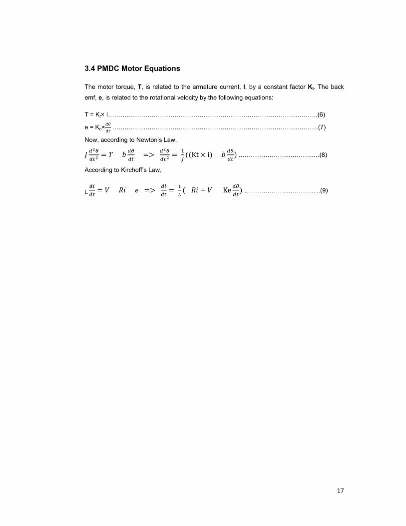
3.4 PMDC Motor Equations

The motor torque, T, is related to the armature current, I, by a constant factor Kt. The back

emf, e, is related to the rotational velocity by the following equations:

T = Kt× I………………………………………………………………………………………..(6)

e = Ke×��

�� ………………………………………………………………………………………(7)

Now, according to Newton’s Law,

��

��= � �

��

�� =>

��

��=

�

�((Kt × i) �

��

��) …………………………………(8)

According to Kirchoff’s Law,

L ��

��= � �� =>

��

��=

�

�( �� + � Ke

��

��) ……………………………....(9)

18

3.5 Simulation with MATLAB Simulink

Figure 3.2 Simulink Block for PID Control of PMDC Motor

Figure 3.2 shows the simulink block for Discrete PID Control of PMDC Motor with zero torque

disturbance. The description of discrete PID Control block is as shown in Figure 3.3.

19

Figure 3.3 PID Control Block

3.5.1 Tuning of Discrete PID Controller

Figure 3.4 Tuning of PID Controller

20

The tuning of a discrete PID Controller in MATLAB Simulink is done as shown in figure 3.4.

The PID Controller can be tuned according to the response time required [11].

3.5.2 Simulation Results

Horizontal X-axis -> time(sec)

Vertical Y-axis -> speed (rpm)

Figure 3.5 Simulation Result

3.5.3 Computed Parameters

Motor Parameters Taken:

- Ra =1 Ohm

- La=0.5 H

- k=0.01 Nm/Amp

- b=0.1 Nms

- J=0.01 kg.m2

Tuned PID Block Parameters:

- Kp =19

- Ki = 43

- Kd = -0.5

- N = 3.4

- Rise Time = 0.4 s

- Settling Time = 1.25 s

- Overshoot = 8.8%

21

CHAPTER 4. MATLAB SIMULINK BASED IMAGE

PROCESSING FOR OBSTACLE

DETECTION

4.1 MATLAB Simulink Model

Figure 4.1 MATLAB Simulink Model for Imgae Processing

Figure 4.1 shows the MATLAB Simulink Model for image processing. A video in “AVI” format

is used as an input. This video contains the information of path of ARV. The video is

converted to Gray scale through MATLAB Simulink block and saved. After that thresholding

operation is applied to the video. As per shown in Figure 4.2, the obstacle is segmented

through thresholding.

4.1.1 RGB to Gray-Scale Conversion

The image conversion from RGB to Gray-scale is done by two different techniques in

MATLAB Simulink. One method is to use the equation for the intensity levels as below:

GR = 0.2989×R + 0.5870×G + 0.1140×B……………………………………………..(10)

Where GR represents the calculated gray level.

22

Figure 4.2 RGB to Gray scale conversion through basic equation

Figure 4.2 shows RGB to Gray scale conversion through basic equation in MATLAB Simulink.

The “OUTPUT” shown in the figure is the final Gray scale converted Video file.

Figure 4.3 Gray Scale converted video frame

Figure 4.3 shows the gray scale converted frame of the video taken by the camera mounted

on ARV.

Other method to convert from RGB to gray scale is to use the built-in “RGB-to-intensity” block

of MATLAB Simulink.

Figure 4.4 RGB-to-intensity converter block

23

Figure 4.5 RGB to Gray scale conversion through built-in block

4.1.2 Thresholding

The next step to be done to the video frame is thresholding operation. The thresholding is

also done with two different techniques. In first technique, the threshold value of the image is

a constant value based on the colour intensity level of the path. The thresholding is done by

comparing the pixel intensity of the video frame with the set threshold value. The model for

implementation of the first method is shown in Figure 4.6.

Figure 4.6 Image Thresholding using constant threshold value

24

The other method for thresholding is to use a built-in “Autothreshold” block as shown in figure

4.7. The Autothreshold model also contains a “Trace Boundaries” block that traces the

boundaries of objects in a binary image BW, in which nonzero pixels belong to an object and

0 pixels constitute the background. Start Pts is a 2xN element matrix where each column

specifies the 0-based row and column coordinates of the initial point on the object boundary

and N is the number of objects. Pts is a 2M-by-N matrix, where M is the Maximum number of

boundary pixels for each object as specified in the mask. Pts holds the 0-based row and

column coordinates of the boundary pixels.

Figure 4.7 Image thresholding using Autothreshold block

Figure 4.8 Function Block Parameters of Autothreshold

4.2 Simulation Results

Figure 4.9 Simulation Result of Image Proces

Figure 4.9 shows the simulation r

are three images in the figure, out of which the rightmost figure shows the original video

frame, the leftmost figure shows the converted gray scaled video frame and the central figure

shows the thresholded video frame.

Figure 4.8 Function Block Parameters of Autothreshold block

4.2 Simulation Results

Simulation Result of Image Processing based obstacle detection

Figure 4.9 shows the simulation result of Image Processing based obstacle detection.


the leftmost figure shows the converted gray scaled video frame and the central figure

shows the thresholded video frame.

25

based obstacle detection

based obstacle detection. There


the leftmost figure shows the converted gray scaled video frame and the central figure

26

(a) (b)

Figure 4.10 (a) Output of First method of thresholding (Constant threshold value) (b) Output of

second method of thresholding (Autothreshold)

Figure 4.10 shows the output of both the thresholding methods applied on the video frame.

The obstacles in the video frame are of white colour. The black colour indicates the path.

27

CHAPTER 5. RESULTS

5.1 PID Controller Module

Motor Parameters Taken:

- Ra =1 Ohm

- La=0.5 H

- k=0.01 Nm/Amp

- b=0.1 Nms

- J=0.01 kg.m2

Tuned PID Block Parameters:

- Kp =19

- Ki = 43

- Kd = -0.5

- N = 3.4

- Rise Time = 0.4 s

- Settling Time = 1.25 s

- Overshoot = 8.8%

5.2 Video Processing Module

(a) (b)

Figure 5.1 (a) Output of First method of thresholding (Constant threshold value) (b) Output of

second method of thresholding (Autothreshold)

Figure 5.1 shows the individual output of both the thresholding methods applied on the video

frame. The obstacles in the video frame are of white colour. The black colour indicates the

path.

28

CHAPTER 6. CONCLUSION AND FUTURE SCOPE

6.1 Conclusion

The design of ARV gives optimum results when the path is straight, single-coloured and the

obstacles are steady. Digital Image Processing based obstacle detection adds more powerful

visibility for ARV than Infrared sensors. The threshoding and region based image

segmentation method gives proper obstacle detection required to drive ARV. By comparing

the two methods of thresholding, it is observed that the constant threshold value method is

more effective than the Autothreshold method if the path is single colored which is the

requirement of ARV. The tuning of a PID Control for PMDC Motor is complex but it can be

done very effectively with MATLAB Simulink if all the five required parameters of Motor

named- Armature Resistance, Armature Inductance, Damping Ratio of Mechanical System,

Electromotive Force Constant and Moment of Inertia are known.

6.2 Future Scope

The obstacle detection and speed control modules have been implemented in MATLAB

Simulink. The next steps to be implemented are:

- Simulation of Obstacle Avoidance Module (as per the proposed method in Section 2.3)

- Implementation of the synchronized Obstacle Detection, Speed Control and Obstacle

Avoidance Modules on TMS320DM6446 DVEVM (Refer Appendix A)

29

APPENDIX A: TMS320DM6446 DIGITAL MEDIA

SYSTEM ON CHIP

Features

- Hybrid SoC consisting of C6446 DSP and ARM926EJ-S GPP

- 513-, 594-MHz C6446 Clock Rates

- 256.5-, 297-MHz ARM926EJ-S Clock Rates

- Eight 32-Bit C6446 Instructions/Cycle

- 4752 C6446 MIPS

Advanced Very-Long-Instruction-Word (VLIW) TMS320C6446 DSP

Core and ARM926EJ-S Core

- Support for 32-bit and 16-bit(Thumb Mode) Instruction Sets for ARM Core

- DSP Instruction Extensions and Single Cycle MAC

- Endianness: Little Endian for ARM and DSP

C6446 L1/L2 Memory Architecture

- 32K-Byte L1P Program RAM/Cache (Direct Mapped)

- 80K-Byte L1D Data RAM/Cache (2-Way Set-Associative)

- 64K-Byte L2 Unified Mapped RAM/Cache (Flexible RAM/Cache Allocation)

ARM9 Memory Architecture

- 16K-Byte Instruction Cache

- 8K-Byte Data Cache

- 16K-Byte RAM

- 8K-Byte ROM

Video Processing Subsystem

Front End Provides:

- CCD and CMOS Imager Interface

- BT.601/BT.656 Digital YCbCr 4:2:2 (8-/16-Bit) Interface

- Preview Engine for Real-Time Image Processing

- Glueless Interface to Common Video Decoders

- Histogram Module

- Auto-Exposure, Auto-White Balance and Auto-Focus Module

- Resize Engine

Resize Images From 1/4x to 4x

Separate Horizontal/Vertical Control

30

Back End Provides:

- Hardware On-Screen Display (OSD)

- Four 54-MHz DACs for a Combination of

Composite NTSC/PAL Video

Luma/Chroma Separate Video (S-video)

Component (YPbPr or RGB) Video (Progressive)

- Digital Output

8-/16-bit YUV or up to 24-Bit RGB

HD Resolution

Up to 2 Video Windows

31

References

[1] Martin Buehler, Karl Lagnemma, Sanjiv Singh- “The DARPA Urban Challenge

Autonomous Vehicles in City Traffic”, Springer Publication, Pages 202-247

[2] Rostam Affendi Hamzah, Hasrul Nisham Rosly, Saad Hamid- “An Obstacle Detection

and Avoidance of A Mobile Robot with Stereo Vision Camera”, 2011 International

Conference on Electronic Devices, Systems and Applications (ICEDSA)

[3] Sumit Badal, Srivinas Ravela, Bruce Draper, Allen Hanson, “A Practical Obstacle

Detection and Avoidance System”, IEEE 1994, pp 97-104

[4] Su Whan Sung,Jietae Lee and In-Buem Lee, “Process Identification and PID Control”,

WILEY Publications, Pages 111-120

[5] Rafael C. Gonzalez, Richard E. Woods- “Digital Image Processing” Second Edition,

Pages 64-66, 567-624

[6] E. R. Davies – “Machine Vision- Theory, Algorithms and Practicalities” Second

Edition, Pages 79-85, 103-128, 437-440

[7] M. Anji Reddy, Y. Hari Shankar- “Textbook of Digital Image Processing”, BS

Publications, Pages 26-53

[8] Xitao Zhang, Yongwei Zhang- “An Obstacle Detection Method based on Machine

Vision”, IEEE 2010

[9] H. Hashimoto, T. Yamaura, M. Higashiguchi- “Detection of Obstacle from Monocular

Vision based on Histogram Matching Method”, IEEE 1996, pp 1047-1051

[10]“Control System Toolbox 9.1” [Online]. Available:

http://www.mathworks.in/help/toolbox/control/control_product_page.html,

July 25. 2012

[11] Dr. M. Meenakshi- “Microprocessor based PID Controller for Speed Control of DC

Motor”, IEEE Computer Society, International Conference on Emerging Trends in

Engineering and Technology, pp 960-965

[12] “PID Control Without Math” by Robert Lacoste, [Online]. Available:

http://itech.fgcu.edu/faculty/zalewski/CDA4170/files/PIDcontrol.pdf

July 25, 2012

[13] “PID Without a PhD” by Tim Wescott, [Online]. Available:

http://igor.chudov.com/manuals/Servo-Tuning/PID-without-a-PhD.pdf

July 25, 2012

32

Publications

1. Vyas Shaunak Agastya, Lovekumar D Thakker, Prof. Amit Patwardhan, “Simulation of

Obstacle Detection and Speed Control for Autonomous Robotic Vehicle”, International

Conference on Computational Vision and Robotics, Organized by IIMT Bhubaneswar,

August 2012 [ In Press ]