Embed Size (px)
DESCRIPTION
A remarkable theorem about definite integrals is that they can be calculated with antiderivatives.
Citation preview
..
Sec on 5.3Evalua ng Definite Integrals
V63.0121.011: Calculus IProfessor Ma hew Leingang
New York University
April 27, 2011

AnnouncementsI Today: 5.3I Thursday/Friday: Quiz on4.1–4.4
I Monday 5/2: 5.4I Wednesday 5/4: 5.5I Monday 5/9: Review andMovie Day!
I Thursday 5/12: FinalExam, 2:00–3:50pm

ObjectivesI Use the Evalua onTheorem to evaluatedefinite integrals.
I Write an deriva ves asindefinite integrals.
I Interpret definiteintegrals as “net change”of a func on over aninterval.
OutlineLast me: The Definite Integral
The definite integral as a limitProper es of the integral
Evalua ng Definite IntegralsExamples
The Integral as Net Change
Indefinite IntegralsMy first table of integrals
Compu ng Area with integrals

The definite integral as a limitDefini onIf f is a func on defined on [a, b], the definite integral of f from a tob is the number ∫ b
af(x) dx = lim
n→∞
n∑i=1
f(ci)∆x
where∆x =b− an
, and for each i, xi = a+ i∆x, and ci is a point in[xi−1, xi].

The definite integral as a limit
TheoremIf f is con nuous on [a, b] or if f has only finitely many jumpdiscon nui es, then f is integrable on [a, b]; that is, the definite
integral∫ b
af(x) dx exists and is the same for any choice of ci.
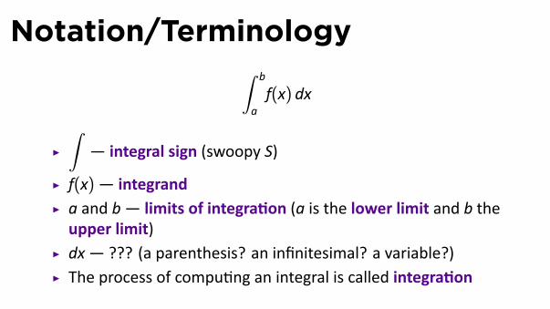
Notation/Terminology∫ b
af(x) dx
I
∫— integral sign (swoopy S)
I f(x)— integrandI a and b— limits of integra on (a is the lower limit and b theupper limit)
I dx— ??? (a parenthesis? an infinitesimal? a variable?)I The process of compu ng an integral is called integra on

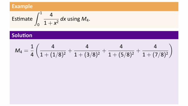
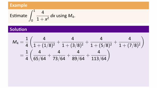
Example
Es mate∫ 1
0
41+ x2
dx usingM4.
Solu on

Example
Es mate∫ 1
0
41+ x2
dx usingM4.
Solu on
We have x0 = 0, x1 =14, x2 =
12, x3 =
34, x4 = 1.
So c1 =18, c2 =
38, c3 =
58, c4 =
78.
Example
Es mate∫ 1
0
41+ x2
dx usingM4.
Solu on
M4 =14
(4
1+ (1/8)2+
41+ (3/8)2
+4
1+ (5/8)2+
41+ (7/8)2
)
=14
(4
65/64+
473/64
+4
89/64+
4113/64
)=
6465
+6473
+6489
+64113
≈ 3.1468
Example
Es mate∫ 1
0
41+ x2
dx usingM4.
Solu on
M4 =14
(4
1+ (1/8)2+
41+ (3/8)2
+4
1+ (5/8)2+
41+ (7/8)2
)=
14
(4
65/64+
473/64
+4
89/64+
4113/64
)
=6465
+6473
+6489
+64113
≈ 3.1468

Example
Es mate∫ 1
0
41+ x2
dx usingM4.
Solu on
M4 =14
(4
1+ (1/8)2+
41+ (3/8)2
+4
1+ (5/8)2+
41+ (7/8)2
)=
14
(4
65/64+
473/64
+4
89/64+
4113/64
)=
6465
+6473
+6489
+64113
≈ 3.1468
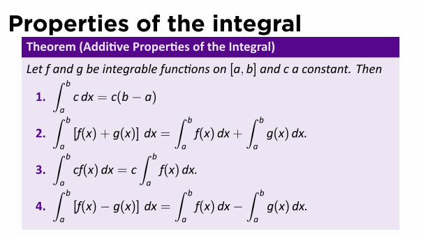
Properties of the integralTheorem (Addi ve Proper es of the Integral)
Let f and g be integrable func ons on [a, b] and c a constant. Then
1.∫ b
ac dx = c(b− a)
2.∫ b
a[f(x) + g(x)] dx =
∫ b
af(x) dx+
∫ b
ag(x) dx.
3.∫ b
acf(x) dx = c
∫ b
af(x) dx.
4.∫ b
a[f(x)− g(x)] dx =
∫ b
af(x) dx−
∫ b
ag(x) dx.

More Properties of the IntegralConven ons: ∫ a
bf(x) dx = −
∫ b
af(x) dx∫ a
af(x) dx = 0
This allows us to haveTheorem
5.∫ c
af(x) dx =
∫ b
af(x) dx+
∫ c
bf(x) dx for all a, b, and c.

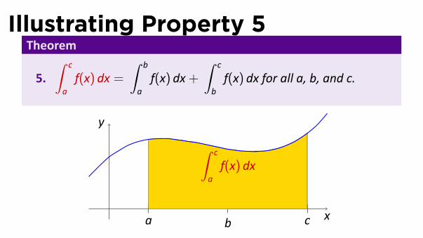
Illustrating Property 5Theorem
5.∫ c
af(x) dx =
∫ b
af(x) dx+
∫ c
bf(x) dx for all a, b, and c.
..x
.
y
..a
..b
..c

Illustrating Property 5Theorem
5.∫ c
af(x) dx =
∫ b
af(x) dx+
∫ c
bf(x) dx for all a, b, and c.
..x
.
y
..a
..b
..c
.
∫ b
af(x) dx

Illustrating Property 5Theorem
5.∫ c
af(x) dx =
∫ b
af(x) dx+
∫ c
bf(x) dx for all a, b, and c.
..x
.
y
..a
..b
..c
.
∫ b
af(x) dx
.
∫ c
bf(x) dx
Illustrating Property 5Theorem
5.∫ c
af(x) dx =
∫ b
af(x) dx+
∫ c
bf(x) dx for all a, b, and c.
..x
.
y
..a
..b
..c
.
∫ b
af(x) dx
.
∫ c
bf(x) dx
.
∫ c
af(x) dx

Illustrating Property 5Theorem
5.∫ c
af(x) dx =
∫ b
af(x) dx+
∫ c
bf(x) dx for all a, b, and c.
..x
.
y
..a..
b..
c

Illustrating Property 5Theorem
5.∫ c
af(x) dx =
∫ b
af(x) dx+
∫ c
bf(x) dx for all a, b, and c.
..x
.
y
..a..
b..
c.
∫ b
af(x) dx
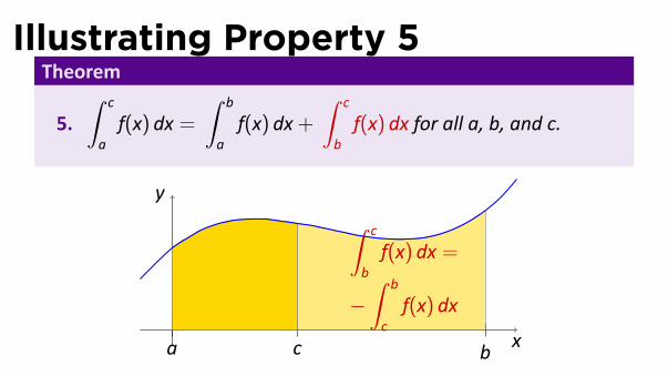
Illustrating Property 5Theorem
5.∫ c
af(x) dx =
∫ b
af(x) dx+
∫ c
bf(x) dx for all a, b, and c.
..x
.
y
..a..
b..
c.
∫ c
bf(x) dx =
−∫ b
cf(x) dx

Illustrating Property 5Theorem
5.∫ c
af(x) dx =
∫ b
af(x) dx+
∫ c
bf(x) dx for all a, b, and c.
..x
.
y
..a..
b..
c.
∫ c
bf(x) dx =
−∫ b
cf(x) dx
.
∫ c
af(x) dx

Definite Integrals We Know So FarI If the integral computes an areaand we know the area, we canuse that. For instance,∫ 1
0
√1− x2 dx =
π
4
I By brute force we computed∫ 1
0x2 dx =
13
∫ 1
0x3 dx =
14
..x
.
y

Comparison Properties of the IntegralTheoremLet f and g be integrable func ons on [a, b].
6. If f(x) ≥ 0 for all x in [a, b], then∫ b
af(x) dx ≥ 0
7. If f(x) ≥ g(x) for all x in [a, b], then∫ b
af(x) dx ≥
∫ b
ag(x) dx
8. If m ≤ f(x) ≤ M for all x in [a, b], then
m(b− a) ≤∫ b
af(x) dx ≤ M(b− a)

Comparison Properties of the IntegralTheoremLet f and g be integrable func ons on [a, b].
6. If f(x) ≥ 0 for all x in [a, b], then∫ b
af(x) dx ≥ 0
7. If f(x) ≥ g(x) for all x in [a, b], then∫ b
af(x) dx ≥
∫ b
ag(x) dx
8. If m ≤ f(x) ≤ M for all x in [a, b], then
m(b− a) ≤∫ b
af(x) dx ≤ M(b− a)

Comparison Properties of the IntegralTheoremLet f and g be integrable func ons on [a, b].
6. If f(x) ≥ 0 for all x in [a, b], then∫ b
af(x) dx ≥ 0
7. If f(x) ≥ g(x) for all x in [a, b], then∫ b
af(x) dx ≥
∫ b
ag(x) dx
8. If m ≤ f(x) ≤ M for all x in [a, b], then
m(b− a) ≤∫ b
af(x) dx ≤ M(b− a)

Comparison Properties of the IntegralTheoremLet f and g be integrable func ons on [a, b].
6. If f(x) ≥ 0 for all x in [a, b], then∫ b
af(x) dx ≥ 0
7. If f(x) ≥ g(x) for all x in [a, b], then∫ b
af(x) dx ≥
∫ b
ag(x) dx
8. If m ≤ f(x) ≤ M for all x in [a, b], then
m(b− a) ≤∫ b
af(x) dx ≤ M(b− a)
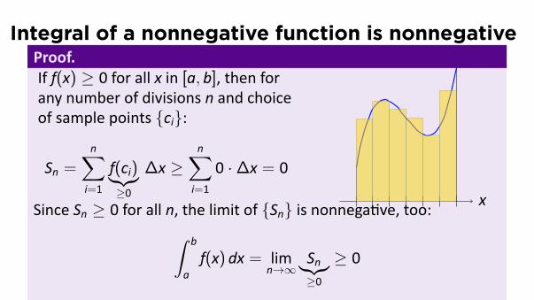
Integral of a nonnegative function is nonnegativeProof.If f(x) ≥ 0 for all x in [a, b], then forany number of divisions n and choiceof sample points {ci}:
Sn =n∑
i=1
f(ci)︸︷︷︸≥0
∆x ≥n∑
i=1
0 ·∆x = 0
.. x.......Since Sn ≥ 0 for all n, the limit of {Sn} is nonnega ve, too:∫ b
af(x) dx = lim
n→∞Sn︸︷︷︸≥0
≥ 0

The integral is “increasing”Proof.Let h(x) = f(x)− g(x). If f(x) ≥ g(x)for all x in [a, b], then h(x) ≥ 0 for allx in [a, b]. So by the previousproperty ∫ b
ah(x) dx ≥ 0 .. x.
f(x)
.
g(x)
.
h(x)
This means that∫ b
af(x) dx−
∫ b
ag(x) dx =
∫ b
a(f(x)− g(x)) dx =
∫ b
ah(x) dx ≥ 0
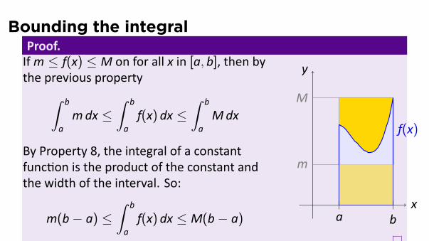
Bounding the integralProof.Ifm ≤ f(x) ≤ M on for all x in [a, b], then bythe previous property∫ b
amdx ≤
∫ b
af(x) dx ≤
∫ b
aMdx
By Property 8, the integral of a constantfunc on is the product of the constant andthe width of the interval. So:
m(b− a) ≤∫ b
af(x) dx ≤ M(b− a)
.. x.
y
.
M
.
f(x)
.
m
..a
..b

Example
Es mate∫ 2
1
1xdx using the comparison proper es.
Solu onSince
12≤ 1
x≤ 1
1for all x in [1, 2], we have
12· 1 ≤
∫ 2
1
1xdx ≤ 1 · 1

Example
Es mate∫ 2
1
1xdx using the comparison proper es.
Solu onSince
12≤ 1
x≤ 1
1for all x in [1, 2], we have
12· 1 ≤
∫ 2
1
1xdx ≤ 1 · 1

Ques on
Es mate∫ 2
1
1xdx with L2 and R2. Are your es mates overes mates?
Underes mates? Impossible to tell?
AnswerSince the integrand is decreasing,
Rn <
∫ 2
1
1xdx < Ln
for all n. So712
<
∫ 2
1
1xdx <
56.

Ques on
Es mate∫ 2
1
1xdx with L2 and R2. Are your es mates overes mates?
Underes mates? Impossible to tell?
AnswerSince the integrand is decreasing,
Rn <
∫ 2
1
1xdx < Ln
for all n. So712
<
∫ 2
1
1xdx <
56.

OutlineLast me: The Definite Integral
The definite integral as a limitProper es of the integral
Evalua ng Definite IntegralsExamples
The Integral as Net Change
Indefinite IntegralsMy first table of integrals
Compu ng Area with integrals
Socratic proofI The definite integral of velocitymeasures displacement (netdistance)
I The deriva ve of displacementis velocity
I So we can computedisplacement with the definiteintegral or the an deriva ve ofvelocity
I But any func on can be avelocity func on, so . . .
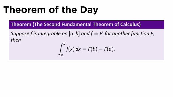
Theorem of the DayTheorem (The Second Fundamental Theorem of Calculus)
Suppose f is integrable on [a, b] and f = F′ for another func on F,then ∫ b
af(x) dx = F(b)− F(a).
NoteIn Sec on 5.3, this theorem is called “The Evalua on Theorem”.Nobody else in the world calls it that.

Theorem of the DayTheorem (The Second Fundamental Theorem of Calculus)
Suppose f is integrable on [a, b] and f = F′ for another func on F,then ∫ b
af(x) dx = F(b)− F(a).
NoteIn Sec on 5.3, this theorem is called “The Evalua on Theorem”.Nobody else in the world calls it that.

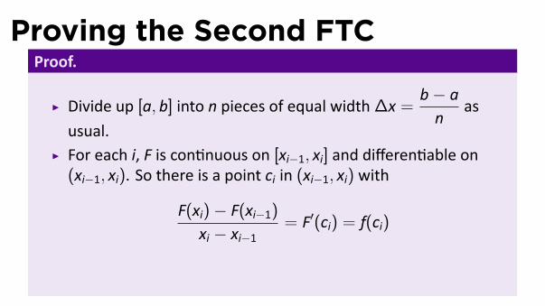
Proving the Second FTCProof.
I Divide up [a, b] into n pieces of equal width∆x =b− an
asusual.
Proving the Second FTCProof.
I Divide up [a, b] into n pieces of equal width∆x =b− an
asusual.
I For each i, F is con nuous on [xi−1, xi] and differen able on(xi−1, xi). So there is a point ci in (xi−1, xi) with
F(xi)− F(xi−1)
xi − xi−1= F′(ci) = f(ci)
= F(xi)− F(xi−1)
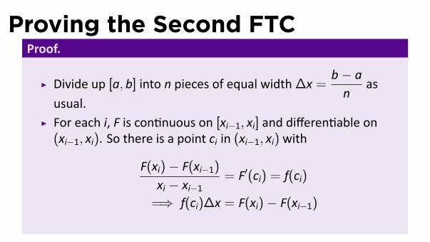
Proving the Second FTCProof.
I Divide up [a, b] into n pieces of equal width∆x =b− an
asusual.
I For each i, F is con nuous on [xi−1, xi] and differen able on(xi−1, xi). So there is a point ci in (xi−1, xi) with
F(xi)− F(xi−1)
xi − xi−1= F′(ci) = f(ci)
=⇒ f(ci)∆x = F(xi)− F(xi−1)

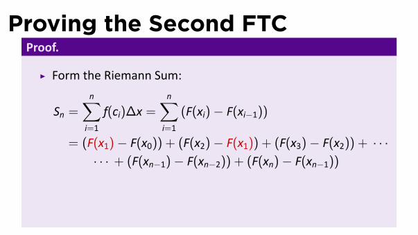
Proving the Second FTCProof.
I Form the Riemann Sum:
Sn =n∑
i=1
f(ci)∆x =n∑
i=1
(F(xi)− F(xi−1))
= (F(x1)− F(x0)) + (F(x2)− F(x1)) + (F(x3)− F(x2)) + · · ·· · · + (F(xn−1)− F(xn−2)) + (F(xn)− F(xn−1))
= F(xn)− F(x0) = F(b)− F(a)

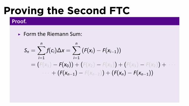
Proving the Second FTCProof.
I Form the Riemann Sum:
Sn =n∑
i=1
f(ci)∆x =n∑
i=1
(F(xi)− F(xi−1))
= (F(x1)− F(x0)) + (F(x2)− F(x1)) + (F(x3)− F(x2)) + · · ·· · · + (F(xn−1)− F(xn−2)) + (F(xn)− F(xn−1))
= F(xn)− F(x0) = F(b)− F(a)

Proving the Second FTCProof.
I Form the Riemann Sum:
Sn =n∑
i=1
f(ci)∆x =n∑
i=1
(F(xi)− F(xi−1))
= (F(x1)− F(x0)) + (F(x2)− F(x1)) + (F(x3)− F(x2)) + · · ·· · · + (F(xn−1)− F(xn−2)) + (F(xn)− F(xn−1))
= F(xn)− F(x0) = F(b)− F(a)
Proving the Second FTCProof.
I Form the Riemann Sum:
Sn =n∑
i=1
f(ci)∆x =n∑
i=1
(F(xi)− F(xi−1))
= (F(x1)− F(x0)) + (F(x2)− F(x1)) + (F(x3)− F(x2)) + · · ·· · · + (F(xn−1)− F(xn−2)) + (F(xn)− F(xn−1))
= F(xn)− F(x0) = F(b)− F(a)

Proving the Second FTCProof.
I Form the Riemann Sum:
Sn =n∑
i=1
f(ci)∆x =n∑
i=1
(F(xi)− F(xi−1))
= (F(x1)− F(x0)) + (F(x2)− F(x1)) + (F(x3)− F(x2)) + · · ·· · · + (F(xn−1)− F(xn−2)) + (F(xn)− F(xn−1))
= F(xn)− F(x0) = F(b)− F(a)

Proving the Second FTCProof.
I Form the Riemann Sum:
Sn =n∑
i=1
f(ci)∆x =n∑
i=1
(F(xi)− F(xi−1))
= (F(x1)− F(x0)) + (F(x2)− F(x1)) + (F(x3)− F(x2)) + · · ·· · · + (F(xn−1)− F(xn−2)) + (F(xn)− F(xn−1))
= F(xn)− F(x0) = F(b)− F(a)

Proving the Second FTCProof.
I Form the Riemann Sum:
Sn =n∑
i=1
f(ci)∆x =n∑
i=1
(F(xi)− F(xi−1))
= (F(x1)− F(x0)) + (F(x2)− F(x1)) + (F(x3)− F(x2)) + · · ·· · · + (F(xn−1)− F(xn−2)) + (F(xn)− F(xn−1))
= F(xn)− F(x0) = F(b)− F(a)

Proving the Second FTCProof.
I Form the Riemann Sum:
Sn =n∑
i=1
f(ci)∆x =n∑
i=1
(F(xi)− F(xi−1))
= (F(x1)− F(x0)) + (F(x2)− F(x1)) + (F(x3)− F(x2)) + · · ·· · · + (F(xn−1)− F(xn−2)) + (F(xn)− F(xn−1))
= F(xn)− F(x0) = F(b)− F(a)

Proving the Second FTCProof.
I Form the Riemann Sum:
Sn =n∑
i=1
f(ci)∆x =n∑
i=1
(F(xi)− F(xi−1))
= (F(x1)− F(x0)) + (F(x2)− F(x1)) + (F(x3)− F(x2)) + · · ·· · · + (F(xn−1)− F(xn−2)) + (F(xn)− F(xn−1))
= F(xn)− F(x0) = F(b)− F(a)

Proving the Second FTCProof.
I Form the Riemann Sum:
Sn =n∑
i=1
f(ci)∆x =n∑
i=1
(F(xi)− F(xi−1))
= (F(x1)− F(x0)) + (F(x2)− F(x1)) + (F(x3)− F(x2)) + · · ·· · · + (F(xn−1)− F(xn−2)) + (F(xn)− F(xn−1))
= F(xn)− F(x0) = F(b)− F(a)
Proving the Second FTCProof.
I Form the Riemann Sum:
Sn =n∑
i=1
f(ci)∆x =n∑
i=1
(F(xi)− F(xi−1))
= (F(x1)− F(x0)) + (F(x2)− F(x1)) + (F(x3)− F(x2)) + · · ·· · · + (F(xn−1)− F(xn−2)) + (F(xn)− F(xn−1))
= F(xn)− F(x0) = F(b)− F(a)

Proving the Second FTCProof.
I Form the Riemann Sum:
Sn =n∑
i=1
f(ci)∆x =n∑
i=1
(F(xi)− F(xi−1))
= (F(x1)− F(x0)) + (F(x2)− F(x1)) + (F(x3)− F(x2)) + · · ·· · · + (F(xn−1)− F(xn−2)) + (F(xn)− F(xn−1))
= F(xn)− F(x0) = F(b)− F(a)

Proving the Second FTCProof.
I Form the Riemann Sum:
Sn =n∑
i=1
f(ci)∆x =n∑
i=1
(F(xi)− F(xi−1))
= (F(x1)− F(x0)) + (F(x2)− F(x1)) + (F(x3)− F(x2)) + · · ·· · · + (F(xn−1)− F(xn−2)) + (F(xn)− F(xn−1))
= F(xn)− F(x0) = F(b)− F(a)

Proving the Second FTCProof.
I Form the Riemann Sum:
Sn =n∑
i=1
f(ci)∆x =n∑
i=1
(F(xi)− F(xi−1))
= (F(x1)− F(x0)) + (F(x2)− F(x1)) + (F(x3)− F(x2)) + · · ·· · · + (F(xn−1)− F(xn−2)) + (F(xn)− F(xn−1))
= F(xn)− F(x0) = F(b)− F(a)
Proving the Second FTCProof.
I We have shown for each n,
Sn = F(b)− F(a)
Which does not depend on n.
I So in the limit∫ b
af(x) dx = lim
n→∞Sn = lim
n→∞(F(b)− F(a)) = F(b)− F(a)

Proving the Second FTCProof.
I We have shown for each n,
Sn = F(b)− F(a)
Which does not depend on n.I So in the limit∫ b
af(x) dx = lim
n→∞Sn = lim
n→∞(F(b)− F(a)) = F(b)− F(a)

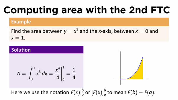
Computing area with the 2nd FTCExample
Find the area between y = x3 and the x-axis, between x = 0 andx = 1.
Solu on
A =
∫ 1
0x3 dx =
x4
4
∣∣∣∣10=
14
.
Here we use the nota on F(x)|ba or [F(x)]ba to mean F(b)− F(a).

Computing area with the 2nd FTCExample
Find the area between y = x3 and the x-axis, between x = 0 andx = 1.
Solu on
A =
∫ 1
0x3 dx =
x4
4
∣∣∣∣10=
14 .
Here we use the nota on F(x)|ba or [F(x)]ba to mean F(b)− F(a).
Computing area with the 2nd FTCExample
Find the area between y = x3 and the x-axis, between x = 0 andx = 1.
Solu on
A =
∫ 1
0x3 dx =
x4
4
∣∣∣∣10=
14 .
Here we use the nota on F(x)|ba or [F(x)]ba to mean F(b)− F(a).

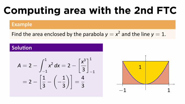
Computing area with the 2nd FTCExample
Find the area enclosed by the parabola y = x2 and the line y = 1.
Solu on
A = 2−∫ 1
−1x2 dx = 2−
[x3
3
]1−1
= 2−[13−
(−13
)]=
43 ...
−1..
1..
1

Computing area with the 2nd FTCExample
Find the area enclosed by the parabola y = x2 and the line y = 1.
Solu on
A = 2−∫ 1
−1x2 dx = 2−
[x3
3
]1−1
= 2−[13−
(−13
)]=
43
...−1
..1
..
1
Computing area with the 2nd FTCExample
Find the area enclosed by the parabola y = x2 and the line y = 1.
Solu on
A = 2−∫ 1
−1x2 dx = 2−
[x3
3
]1−1
= 2−[13−
(−13
)]=
43 ...
−1..
1..
1

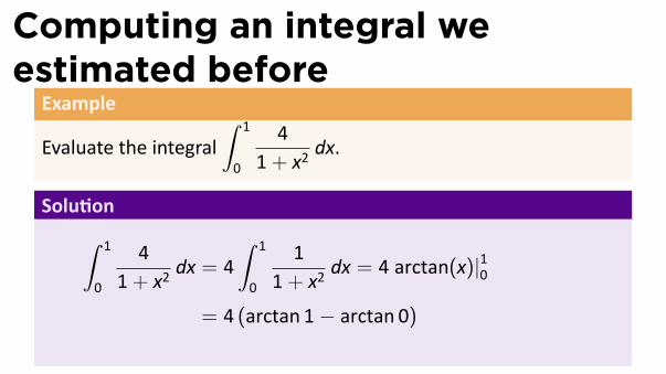
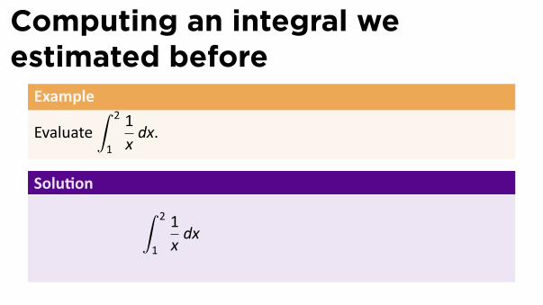
Computing an integral weestimated before
Example
Evaluate the integral∫ 1
0
41+ x2
dx.
Solu on∫ 1
0
41+ x2
dx = 4∫ 1
0
11+ x2
dx
= 4 arctan(x)|10
= 4 (arctan 1− arctan 0) = 4(π4− 0
)
= π

Example
Es mate∫ 1
0
41+ x2
dx usingM4.
Solu on
M4 =14
(4
1+ (1/8)2+
41+ (3/8)2
+4
1+ (5/8)2+
41+ (7/8)2
)=
14
(4
65/64+
473/64
+4
89/64+
4113/64
)=
6465
+6473
+6489
+64113
≈ 3.1468

Computing an integral weestimated before
Example
Evaluate the integral∫ 1
0
41+ x2
dx.
Solu on∫ 1
0
41+ x2
dx = 4∫ 1
0
11+ x2
dx
= 4 arctan(x)|10
= 4 (arctan 1− arctan 0) = 4(π4− 0
)
= π

Computing an integral weestimated before
Example
Evaluate the integral∫ 1
0
41+ x2
dx.
Solu on∫ 1
0
41+ x2
dx = 4∫ 1
0
11+ x2
dx = 4 arctan(x)|10
= 4 (arctan 1− arctan 0) = 4(π4− 0
)
= π
Computing an integral weestimated before
Example
Evaluate the integral∫ 1
0
41+ x2
dx.
Solu on∫ 1
0
41+ x2
dx = 4∫ 1
0
11+ x2
dx = 4 arctan(x)|10
= 4 (arctan 1− arctan 0)
= 4(π4− 0
)
= π

Computing an integral weestimated before
Example
Evaluate the integral∫ 1
0
41+ x2
dx.
Solu on∫ 1
0
41+ x2
dx = 4∫ 1
0
11+ x2
dx = 4 arctan(x)|10
= 4 (arctan 1− arctan 0) = 4(π4− 0
)
= π

Computing an integral weestimated before
Example
Evaluate the integral∫ 1
0
41+ x2
dx.
Solu on∫ 1
0
41+ x2
dx = 4∫ 1
0
11+ x2
dx = 4 arctan(x)|10
= 4 (arctan 1− arctan 0) = 4(π4− 0
)= π

Computing an integral weestimated before
Example
Evaluate∫ 2
1
1xdx.
Solu on ∫ 2
1
1xdx
= ln x|21 = ln 2− ln 1 = ln 2

Example
Es mate∫ 2
1
1xdx using the comparison proper es.
Solu onSince
12≤ 1
x≤ 1
1for all x in [1, 2], we have
12· 1 ≤
∫ 2
1
1xdx ≤ 1 · 1
Computing an integral weestimated before
Example
Evaluate∫ 2
1
1xdx.
Solu on ∫ 2
1
1xdx
= ln x|21 = ln 2− ln 1 = ln 2

Computing an integral weestimated before
Example
Evaluate∫ 2
1
1xdx.
Solu on ∫ 2
1
1xdx = ln x|21
= ln 2− ln 1 = ln 2

Computing an integral weestimated before
Example
Evaluate∫ 2
1
1xdx.
Solu on ∫ 2
1
1xdx = ln x|21 = ln 2− ln 1
= ln 2

Computing an integral weestimated before
Example
Evaluate∫ 2
1
1xdx.
Solu on ∫ 2
1
1xdx = ln x|21 = ln 2− ln 1 = ln 2

OutlineLast me: The Definite Integral
The definite integral as a limitProper es of the integral
Evalua ng Definite IntegralsExamples
The Integral as Net Change
Indefinite IntegralsMy first table of integrals
Compu ng Area with integrals
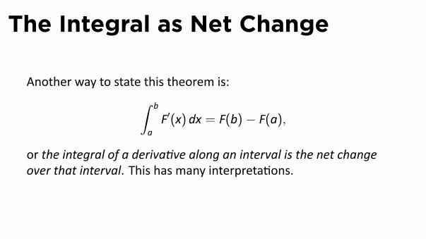
The Integral as Net Change
Another way to state this theorem is:∫ b
aF′(x) dx = F(b)− F(a),
or the integral of a deriva ve along an interval is the net changeover that interval. This has many interpreta ons.

The Integral as Net Change
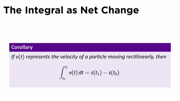
The Integral as Net Change
Corollary
If v(t) represents the velocity of a par cle moving rec linearly, then∫ t1
t0v(t) dt = s(t1)− s(t0).

The Integral as Net Change
Corollary
If MC(x) represents the marginal cost of making x units of a product,then
C(x) = C(0) +∫ x
0MC(q) dq.
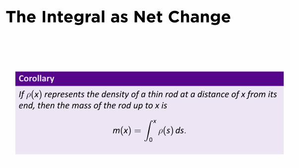
The Integral as Net Change
Corollary
If ρ(x) represents the density of a thin rod at a distance of x from itsend, then the mass of the rod up to x is
m(x) =∫ x
0ρ(s) ds.

OutlineLast me: The Definite Integral
The definite integral as a limitProper es of the integral
Evalua ng Definite IntegralsExamples
The Integral as Net Change
Indefinite IntegralsMy first table of integrals
Compu ng Area with integrals

A new notation for antiderivativesTo emphasize the rela onship between an differen a on andintegra on, we use the indefinite integral nota on∫
f(x) dx
for any func on whose deriva ve is f(x).
Thus∫x2 dx = 1
3x3 + C.

A new notation for antiderivativesTo emphasize the rela onship between an differen a on andintegra on, we use the indefinite integral nota on∫
f(x) dx
for any func on whose deriva ve is f(x). Thus∫x2 dx = 1
3x3 + C.

My first table of integrals..∫
[f(x) + g(x)] dx =∫
f(x) dx+∫
g(x) dx∫xn dx =
xn+1
n+ 1+ C (n ̸= −1)∫
ex dx = ex + C∫sin x dx = − cos x+ C∫cos x dx = sin x+ C∫sec2 x dx = tan x+ C∫
sec x tan x dx = sec x+ C∫1
1+ x2dx = arctan x+ C
∫cf(x) dx = c
∫f(x) dx∫
1xdx = ln |x|+ C∫
ax dx =ax
ln a+ C∫
csc2 x dx = − cot x+ C∫csc x cot x dx = − csc x+ C∫
1√1− x2
dx = arcsin x+ C

OutlineLast me: The Definite Integral
The definite integral as a limitProper es of the integral
Evalua ng Definite IntegralsExamples
The Integral as Net Change
Indefinite IntegralsMy first table of integrals
Compu ng Area with integrals

Computing Area with integrals
Example
Find the area of the region bounded by the lines x = 1, x = 4, thex-axis, and the curve y = ex.
Solu onThe answer is ∫ 4
1ex dx = ex|41 = e4 − e.

Computing Area with integrals
Example
Find the area of the region bounded by the lines x = 1, x = 4, thex-axis, and the curve y = ex.
Solu onThe answer is ∫ 4
1ex dx = ex|41 = e4 − e.

Computing Area with integralsExample
Find the area of the region bounded by the curve y = arcsin x, thex-axis, and the line x = 1.
Solu on
I Instead compute the area as
π
2−∫ π/2
0sin y dy =
π
2−[− cos x]π/20 =
π
2−1
..x
.
y
..1
..
π/2

Computing Area with integralsExample
Find the area of the region bounded by the curve y = arcsin x, thex-axis, and the line x = 1.
Solu on
I The answer is∫ 1
0arcsin x dx, but
we do not know an an deriva vefor arcsin.
I Instead compute the area as
π
2−∫ π/2
0sin y dy =
π
2−[− cos x]π/20 =
π
2−1
..x
.
y
..1
..
π/2

Computing Area with integralsExample
Find the area of the region bounded by the curve y = arcsin x, thex-axis, and the line x = 1.
Solu on
I Instead compute the area as
π
2−∫ π/2
0sin y dy
=π
2−[− cos x]π/20 =
π
2−1
..x
.
y
..1
..
π/2

Computing Area with integralsExample
Find the area of the region bounded by the curve y = arcsin x, thex-axis, and the line x = 1.
Solu on
I Instead compute the area as
π
2−∫ π/2
0sin y dy =
π
2−[− cos x]π/20
=π
2−1
..x
.
y
..1
..
π/2

Computing Area with integralsExample
Find the area of the region bounded by the curve y = arcsin x, thex-axis, and the line x = 1.
Solu on
I Instead compute the area as
π
2−∫ π/2
0sin y dy =
π
2−[− cos x]π/20 =
π
2−1
..x
.
y
..1
..
π/2

Example
Find the area between the graph of y = (x− 1)(x− 2), the x-axis,and the ver cal lines x = 0 and x = 3.
Solu on
.. x.
y
..1
..2
..3

Example
Find the area between the graph of y = (x− 1)(x− 2), the x-axis,and the ver cal lines x = 0 and x = 3.
Solu onNo ce the func ony = (x− 1)(x− 2) is posi ve on [0, 1)and (2, 3], and nega ve on (1, 2).
.. x.
y
..1
..2
..3
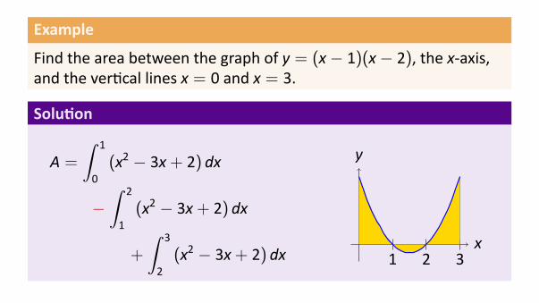
Example
Find the area between the graph of y = (x− 1)(x− 2), the x-axis,and the ver cal lines x = 0 and x = 3.
Solu on
A =
∫ 1
0(x2 − 3x+ 2) dx
−∫ 2
1(x2 − 3x+ 2) dx
+
∫ 3
2(x2 − 3x+ 2) dx
.. x.
y
..1
..2
..3
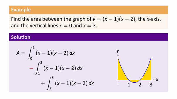
Example
Find the area between the graph of y = (x− 1)(x− 2), the x-axis,and the ver cal lines x = 0 and x = 3.
Solu on
A =
∫ 1
0(x− 1)(x− 2) dx
−∫ 2
1(x− 1)(x− 2) dx
+
∫ 3
2(x− 1)(x− 2) dx
.. x.
y
..1
..2
..3

Example
Find the area between the graph of y = (x− 1)(x− 2), the x-axis,and the ver cal lines x = 0 and x = 3.
Solu on
A =[13x
3 − 32x
2 + 2x]10
−[13x
3 − 32x
2 + 2x]21
+[13x
3 − 32x
2 + 2x]32
=116
.. x.
y
..1
..2
..3

Interpretation of “negative area”in motion
There is an analog in rectlinear mo on:
I
∫ t1
t0v(t) dt is net distance traveled.
I
∫ t1
t0|v(t)| dt is total distance traveled.

What about the constant?I It seems we forgot about the+C when we say for instance∫ 1
0x3 dx =
x4
4
∣∣∣∣10=
14− 0 =
14
I But no ce[x4
4+ C
]10=
(14+ C
)− (0+ C) =
14+ C− C =
14
no ma er what C is.I So in an differen a on for definite integrals, the constant isimmaterial.
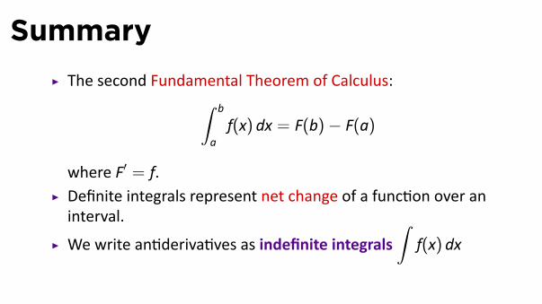
SummaryI The second Fundamental Theorem of Calculus:∫ b
af(x) dx = F(b)− F(a)
where F′ = f.I Definite integrals represent net change of a func on over aninterval.
I We write an deriva ves as indefinite integrals∫
f(x) dx