Geometry of Continuous-Time Markov Chains

Shuchang Zhang

Content

› Motivation

› Mathematical Background

› Geometric Flow of Markov Chain

› Conclusions

Motivation

Motivation

• Time reversible Markov chain (detailed balance) is known to havesymmetric probability flux and can be described by gradient system

• Symmetric flux contributes to the production of relative entropy,whereas skew-symmetric flux doesn’t

• Skew-symmetric flux playing a very important role as circulation intime evolution of chains is yet hardly understood

• Evolution of Markov chain can be characterized by differentialgeometry, which is a powerful and indispensable tool in dynamics

Mathematical Background

Alpha representation

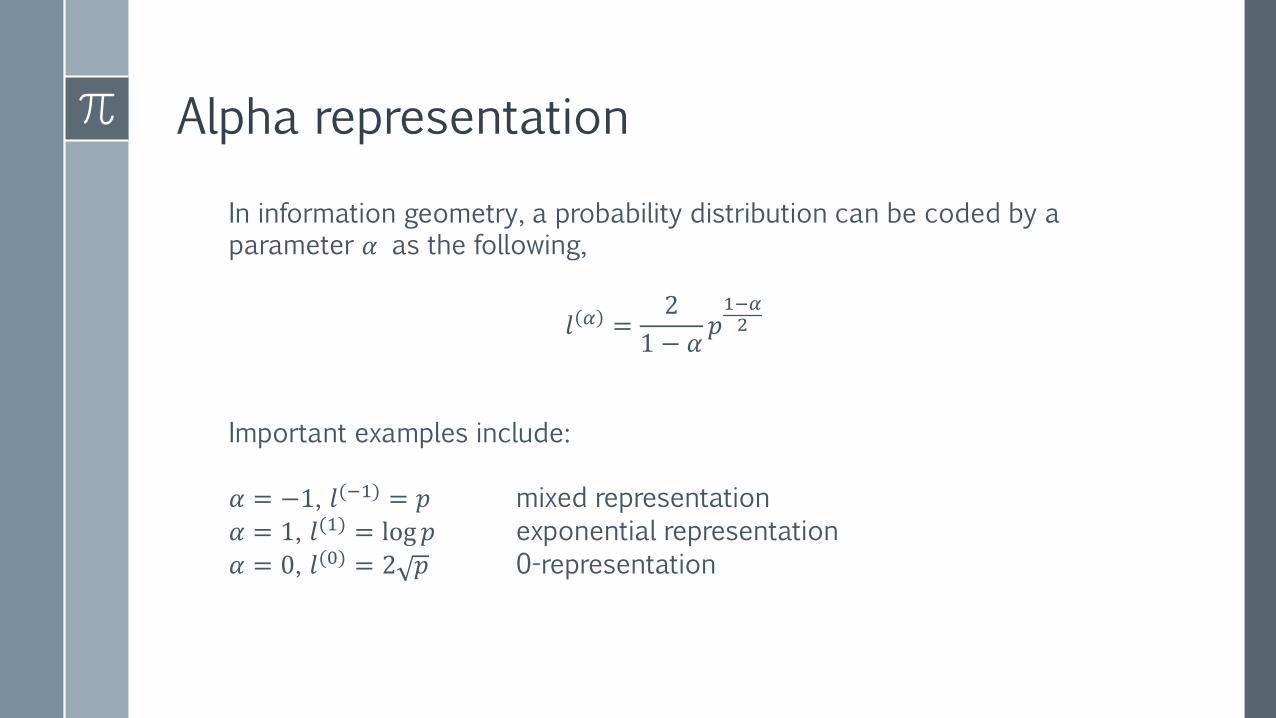
In information geometry, a probability distribution can be coded by a parameter 𝛼 as the following,

𝑙 𝛼 =2

1 − 𝛼𝑝1−𝛼2

Important examples include:

𝛼 = −1, 𝑙(−1) = 𝑝 mixed representation

𝛼 = 1, 𝑙(1) = log𝑝 exponential representation

𝛼 = 0, 𝑙(0) = 2 𝑝 0-representation

Alpha representation

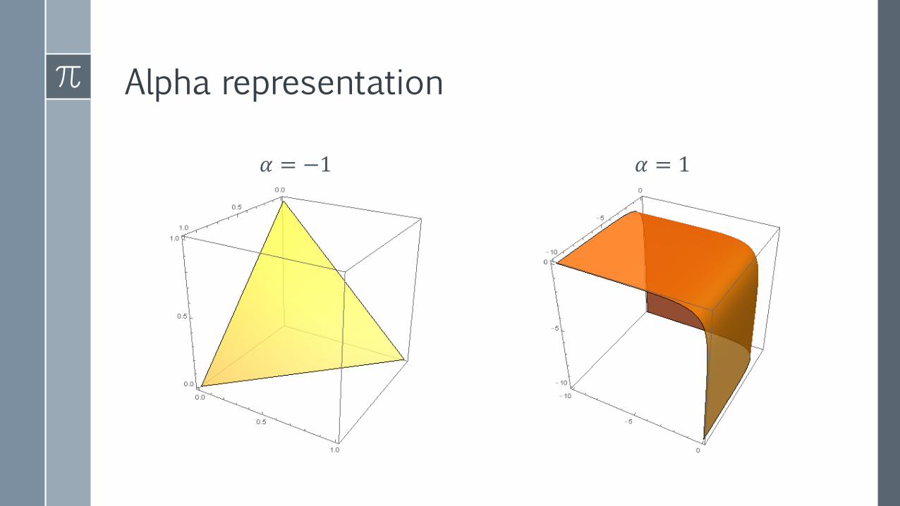
𝛼 = −1 𝛼 = 1

Alpha representation

𝛼 = −1 𝛼 = 0

Alpha representation

• Different representations are equipped with different geometric structures and restrict the dynamics of Markov chains on different manifolds.

• Particularly, 0-representation admits the flow of probability on the (hyper)sphere, which has radical symmetry.

Lie group of 𝑆𝑂𝑛

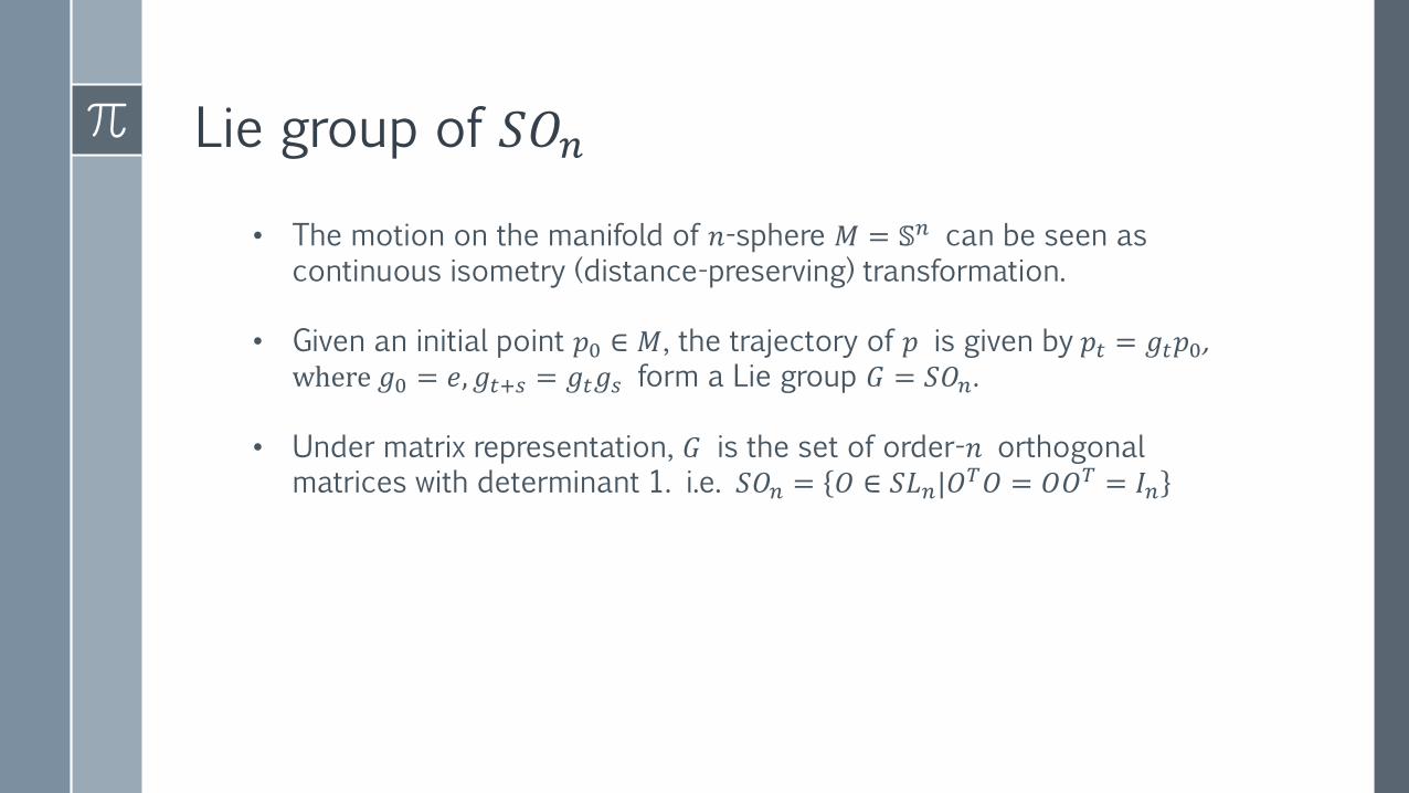
• The motion on the manifold of 𝑛-sphere 𝑀 = 𝕊𝑛 can be seen as continuous isometry (distance-preserving) transformation.

• Given an initial point 𝑝0 ∈ 𝑀, the trajectory of 𝑝 is given by 𝑝𝑡 = 𝑔𝑡𝑝0,where 𝑔0 = 𝑒, 𝑔𝑡+𝑠 = 𝑔𝑡𝑔𝑠 form a Lie group 𝐺 = 𝑆𝑂𝑛.

• Under matrix representation, 𝐺 is the set of order-𝑛 orthogonal matrices with determinant 1. i.e. 𝑆𝑂𝑛 = 𝑂 ∈ 𝑆𝐿𝑛|𝑂

𝑇𝑂 = 𝑂𝑂𝑇 = 𝐼𝑛

Lie algebra of 𝔰𝔬𝑛

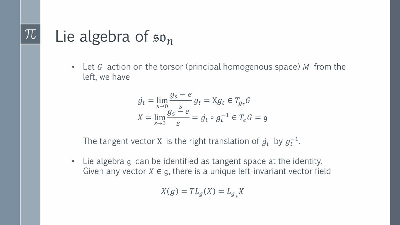
• Let 𝐺 action on the torsor (principal homogenous space) 𝑀 from the left, we have

ሶ𝑔𝑡 = lim𝑠→0

𝑔𝑠 − 𝑒

𝑠𝑔𝑡 = X𝑔𝑡 ∈ 𝑇𝑔𝑡𝐺

𝑋 = lim𝑠→0

𝑔s − 𝑒

𝑠= ሶ𝑔𝑡 ∘ 𝑔𝑡

−1 ∈ 𝑇𝑒𝐺 = 𝔤

The tangent vector X is the right translation of ሶ𝑔𝑡 by 𝑔𝑡−1.

• Lie algebra 𝔤 can be identified as tangent space at the identity. Given any vector 𝑋 ∈ 𝔤, there is a unique left-invariant vector field

𝑋 𝑔 = 𝑇𝐿𝑔 𝑋 = 𝐿𝑔∗𝑋

Lie algebra of 𝔰𝔬𝑛

• Note that for 𝑂𝑠 ∈ 𝑆𝑂𝑛 near the identity, we have

𝐼 = 𝑂𝑠𝑇𝑂𝑠 = 𝐼 + 𝑠Ω + 𝑜 𝑠

𝑇𝐼 + 𝑠Ω + 𝑜 𝑠 = 𝐼 + 𝑠 Ω + Ω𝑇 + 𝑜 𝑠

The matrix Lie algebra of 𝔰𝔬𝑛 is the set of skew-symmetric matrices, i.e. 𝔰𝔬𝑛 = 𝑇𝑒𝑆𝑂𝑛 = Ω ∈ 𝐺𝐿𝑛| Ω + Ω𝑇 = 0

• It can also be identified with vector space of dimension 𝑛(𝑛−1)

2

Adjoint and coadjoint representation of 𝔰𝔬𝑛

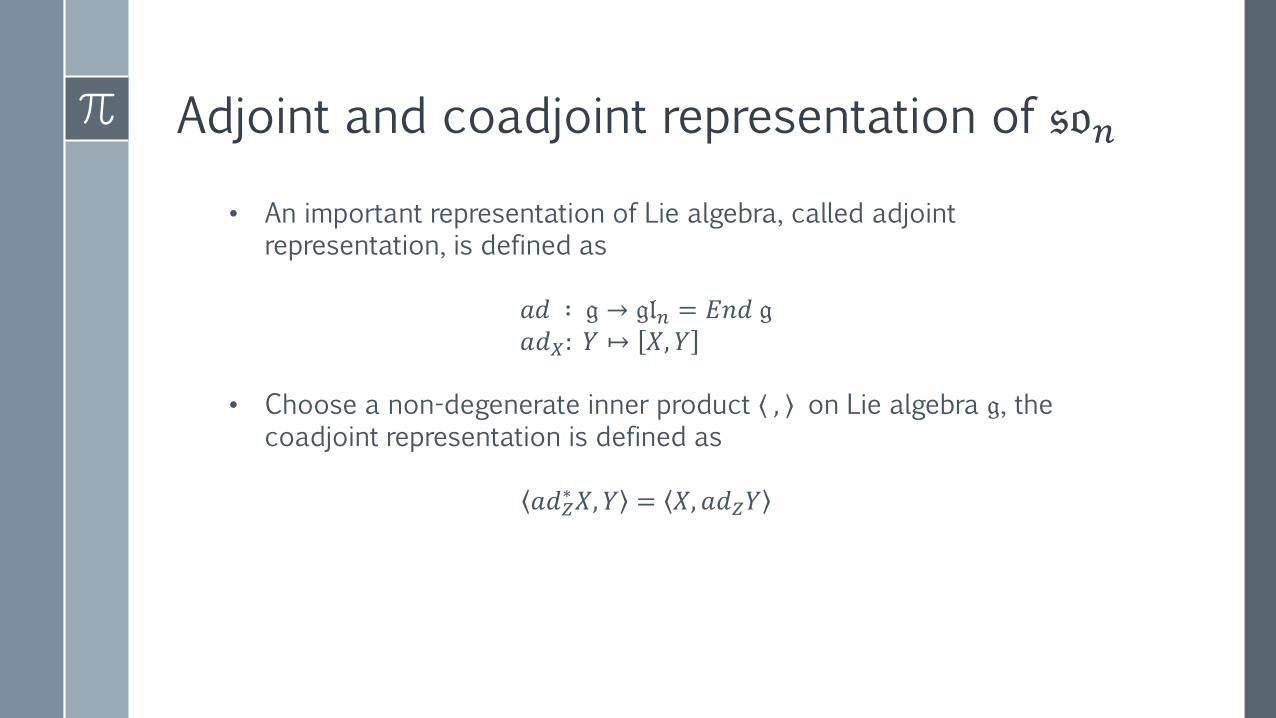
• An important representation of Lie algebra, called adjointrepresentation, is defined as

𝑎𝑑 ∶ 𝔤 → 𝔤𝔩𝑛 = 𝐸𝑛𝑑 𝔤𝑎𝑑𝑋: 𝑌 ↦ 𝑋, 𝑌

• Choose a non-degenerate inner product , on Lie algebra 𝔤, the coadjoint representation is defined as

𝑎𝑑𝑍∗𝑋, 𝑌 = 𝑋, 𝑎𝑑𝑍𝑌

Riemannian metric

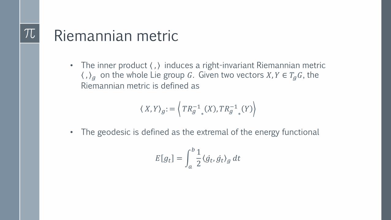
• The inner product , induces a right-invariant Riemannian metric , 𝑔 on the whole Lie group 𝐺. Given two vectors 𝑋, 𝑌 ∈ 𝑇𝑔𝐺, the

Riemannian metric is defined as

𝑋, 𝑌 𝑔: = 𝑇𝑅𝑔−1

∗𝑋 , 𝑇𝑅𝑔

−1∗𝑌

• The geodesic is defined as the extremal of the energy functional

𝐸 𝑔𝑡 = න𝑎

𝑏 1

2ሶ𝑔𝑡, ሶ𝑔𝑡 𝑔 𝑑𝑡

Geometric Flow of Markov Chain

0-representation of Markov chain

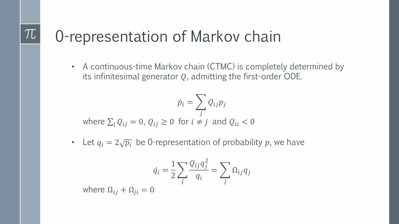
• A continuous-time Markov chain (CTMC) is completely determined by its infinitesimal generator 𝑄, admitting the first-order ODE.

ሶ𝑝𝑖 =

𝑗

𝑄𝑖𝑗𝑝𝑗

where σ𝑖𝑄𝑖𝑗 = 0, 𝑄𝑖𝑗 ≥ 0 for 𝑖 ≠ 𝑗 and 𝑄𝑖𝑖 < 0

• Let 𝑞𝑖 = 2 𝑝𝑖 be 0-representation of probability 𝑝, we have

ሶ𝑞𝑖 =1

2

𝑗

𝑄𝑖𝑗𝑞𝑗2

𝑞𝑖=

𝑗

Ω𝑖𝑗𝑞𝑗

where Ω𝑖𝑗 + Ω𝑗𝑖 = 0

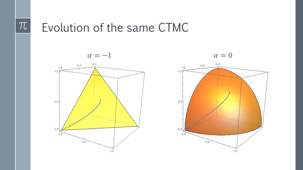
Evolution of the same CTMC

𝛼 = −1 𝛼 = 0

Geometric flow of CTMC

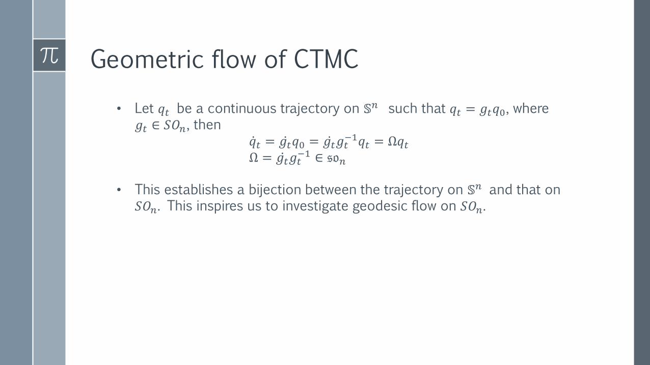
• Let 𝑞𝑡 be a continuous trajectory on 𝕊𝑛 such that 𝑞𝑡 = 𝑔𝑡𝑞0, where 𝑔𝑡 ∈ 𝑆𝑂𝑛, then

ሶ𝑞𝑡 = ሶ𝑔𝑡𝑞0 = ሶ𝑔𝑡𝑔𝑡−1𝑞𝑡 = Ω𝑞𝑡

Ω = ሶ𝑔𝑡𝑔𝑡−1 ∈ 𝔰𝔬𝑛

• This establishes a bijection between the trajectory on 𝕊𝑛 and that on 𝑆𝑂𝑛. This inspires us to investigate geodesic flow on 𝑆𝑂𝑛.

Geodesic flow on 𝑆𝑂𝑛

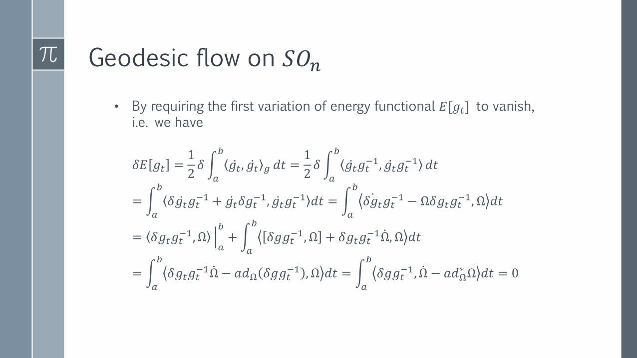
• By requiring the first variation of energy functional 𝐸[𝑔𝑡] to vanish, i.e. we have

𝛿𝐸 𝑔𝑡 =1

2𝛿 න

𝑎

𝑏

ሶ𝑔𝑡 , ሶ𝑔𝑡 𝑔 𝑑𝑡 =1

2𝛿 න

𝑎

𝑏

ሶ𝑔𝑡𝑔𝑡−1, ሶ𝑔𝑡𝑔𝑡

−1 𝑑𝑡

= න𝑎

𝑏

𝛿 ሶ𝑔𝑡𝑔𝑡−1 + ሶ𝑔𝑡𝛿𝑔𝑡

−1, ሶ𝑔𝑡𝑔𝑡−1 𝑑𝑡 = න

𝑎

𝑏ሶ𝛿𝑔𝑡𝑔𝑡

−1 − Ω𝛿𝑔𝑡𝑔𝑡−1, Ω 𝑑𝑡

= 𝛿𝑔𝑡𝑔𝑡−1, Ω ቚ

𝑎

𝑏+න

𝑎

𝑏

𝛿𝑔𝑔𝑡−1, Ω + 𝛿𝑔𝑡𝑔𝑡

−1 ሶΩ, Ω 𝑑𝑡

= න𝑎

𝑏

𝛿𝑔𝑡𝑔𝑡−1 ሶΩ − 𝑎𝑑Ω 𝛿𝑔𝑔𝑡

−1 , Ω 𝑑𝑡 = න𝑎

𝑏

𝛿𝑔𝑔𝑡−1, ሶΩ − 𝑎𝑑Ω

∗ Ω 𝑑𝑡 = 0

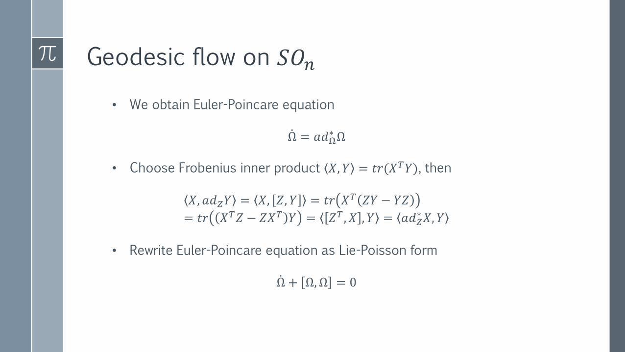
Geodesic flow on 𝑆𝑂𝑛

• We obtain Euler-Poincare equation

ሶΩ = 𝑎𝑑Ω∗ Ω

• Choose Frobenius inner product 𝑋, 𝑌 = 𝑡𝑟(𝑋𝑇𝑌), then

𝑋, 𝑎𝑑𝑍𝑌 = 𝑋, 𝑍, 𝑌 = 𝑡𝑟 𝑋𝑇 𝑍𝑌 − 𝑌𝑍

= 𝑡𝑟 𝑋𝑇𝑍 − 𝑍𝑋𝑇 𝑌 = 𝑍𝑇 , 𝑋 , 𝑌 = 𝑎𝑑𝑍∗𝑋, 𝑌

• Rewrite Euler-Poincare equation as Lie-Poisson form

ሶΩ + Ω, Ω = 0

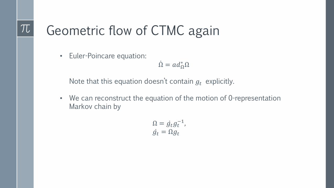
Geometric flow of CTMC again

• Euler-Poincare equation:ሶΩ = 𝑎𝑑Ω

∗ Ω

Note that this equation doesn’t contain 𝑔𝑡 explicitly.

• We can reconstruct the equation of the motion of 0-representation Markov chain by

Ω = ሶ𝑔𝑡𝑔𝑡−1,

ሶ𝑔𝑡 = Ω𝑔𝑡

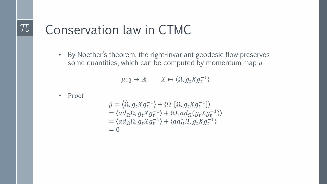
Conservation law in CTMC

• By Noether’s theorem, the right-invariant geodesic flow preserves some quantities, which can be computed by momentum map 𝜇

𝜇: 𝔤 → ℝ, 𝑋 ↦ Ω, 𝑔𝑡𝑋𝑔𝑡−1

• Proof

ሶ𝜇 = ሶΩ, 𝑔𝑡𝑋𝑔𝑡−1 + Ω, Ω, 𝑔𝑡𝑋𝑔𝑡

−1

= 𝑎𝑑ΩΩ, 𝑔𝑡𝑋𝑔𝑡−1 + Ω, 𝑎𝑑Ω 𝑔𝑡𝑋𝑔𝑡

−1

= 𝑎𝑑ΩΩ, 𝑔𝑡𝑋𝑔𝑡−1 + 𝑎𝑑Ω

∗ 𝛺, 𝑔𝑡𝑋𝑔𝑡−1

= 0

Conclusions

Conclusions

In summary, we give a geometric formulation of 0-representation CTMC. This view allows us to

• Investigate the dynamics on (hyper)sphere, from both intrinsic and extrinsic view

• Reduce the dimension of infinitesimal generator by half (from

𝑛(𝑛 − 1) to 𝑛 𝑛−1

2)

• The time evolution of Markov chains follows Euler-Poincare equation, whose trajectory is always geodesic flow

• Conservation quantities can be found

Further questions

There are many problems to be solved yet

• How to distinguish skew-symmetric flux from symmetric one in geometric view

• Geometric formulation of CTMC in other representations

• Find master equation of geodesic flows

• Etc..