Embed Size (px)
Citation preview

Case Study 1 Adaptive Phase 2 Design in post‐surgical painp g p g p
Proof‐of‐Concept & Dose‐Exploration Stage A Maximizing Dose‐Finding Design Stage B
Jim Bolognese, CytelEAST UGM22Oct201422Oct2014

OUTLINEOUTLINE
• Adaptive design based on customized clinicalAdaptive design based on customized clinical utility function
• Simulation results document performance• Simulation results document performance characteristicsR k• Remarks

Overall Summary• Phase 2 trial test drug versus placebo and active control for post surgery• Phase 2 trial test drug versus placebo and active control for post‐surgery
analgesia• Objectives: PoC + estimate dose regimen with optimal balance between
maximum efficacy and minimum intolerance• Maximizing adaptive dose‐finding design (Ivanova, 2009) chosen to yield
better quality information– fewer patients assigned to dose regimens which are ineffective or
intolerableintolerable• True potential efficacy and tolerability dose‐response (DR) curves were
constructed to span the range of potential DR curves• Clinical utility function defined to combine all of the efficacy and
t l bilit dtolerability dose‐response curves• Simulation study evaluated performance characteristics• Results indicate the maximizing design
– Has high probability to estimate the correct or nearest to correct dose– Has high probability to estimate the correct or nearest to correct dose with maximum clinical utility (i.e., “target dose”)
– Maximizes assignment of subjects to the target dose– Minimizes assignment of subject to doses remote from target dose

Illustration of Maximizing Design(Ivanova et al 2009)Current cohort Next cohort(Ivanova et al. 2009)
Doses 1 2 3 4 1 2 3 4Active pair
At given point of the study subjects are randomized to the levels of the
Active pairof levels
At given point of the study, subjects are randomized to the levels of the current dose pair and placebo only. The next pair is obtained by shifting the current pair according to the estimated slope.

Maximizing Design Update Rule based on Standarized Difference
)/1/1(ˆ)ˆˆ(
21 jj
nnT
)/1/1( 1 jj nn
Let dose j and j+1 constitute the current dose pair.1 Use isotonic (unimodal) regression or quadratic regression fitted locally1. Use isotonic (unimodal) regression or quadratic regression fitted locally
to estimate responses at all dose levels using all available data2. Compute T
i. If T > 0.3 then next dose pair (j+1,j+2), i.e. "move up“p (j ,j ), pii. If T < ‐0.3 then next dose pair ( j‐1, j), i.e. "move down“iii. Otherwise, next dose pair ( j, j+1), i.e. “stay”• If not possible to “move” dose pair, ( j=1 or j=K‐1), change pair’s
randomization probabilities from 1:1 to 2:1 (the extreme dose of the pair get twice more subjects)
M difi i f hi l (i l di diff ff f T) iblModification of this rule (including different cutoffs for T) are possible but logic is similar

Final Phase 2 Design Choice:2‐Stage adaptive PoC+Dose‐Findingg p g
• Stage A ‐ PoC: Initial Cohort of 150 patients randomized 1:1:1:1:1:1 to 1 of 4 Test Drug regimens; active control; placebo)
• Enrollment pause for ~1 month while Stage A data are analyzed• Stage B – Dose‐Finding: Maximizing Design for clinical utility; 2 starting
doses based on the analysis of Stage A– Patients randomized in ~10 successive weekly cohorts of
approximately 25 patients (depending on weekly enrollment rate)– Each successive Stage B cohort of ~25 will be randomized 4:8:8:5 to g
placebo, 2 doses of Test Drug, and active control, respectively– Expected to yield for final analysis ~
• 65 total placebo patients65 total placebo patients• 75 total active control patients• > 80‐100 patients on target dose

Potential utility outcomef hfor each Test Drug group
← Increasing Test Drug Tolerability
IncreasingTest Drug
AC<T~plc AC<T<plc AC~T<plc T<AC<plc
AC>T~plc 0
AC>T>plcgEfficacy↓
AC>T>plc
AC~T>plc
T>AC>plc 100
Utility ranges from 0‐100 higher is betterUtility ranges from 0‐100, higher is better
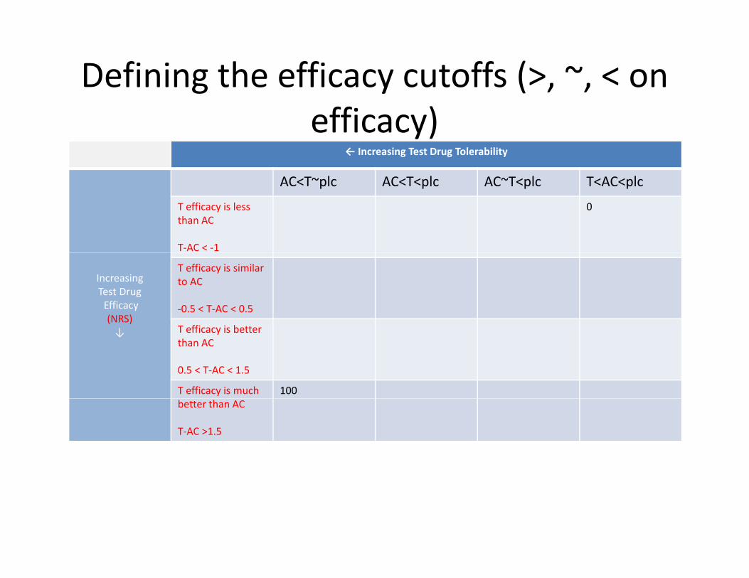
Defining the efficacy cutoffs (>, ~, < on ff )efficacy)
← Increasing Test Drug Tolerability
AC<T~plc AC<T<plc AC~T<plc T<AC<plcAC<T~plc AC<T<plc AC~T<plc T<AC<plc
T efficacy is less than AC
T‐AC < ‐1
0
IncreasingTest DrugEfficacy(NRS)
T efficacy is similar to AC
‐0.5 < T‐AC < 0.5
T ffi i b↓ T efficacy is better than AC
0.5 < T‐AC < 1.5
T efficacy is much 100better than AC
T‐AC >1.5

Defining the tolerability cutoffs( l b l )(>, ~, < on tolerability)
← Increasing Test Drug Tolerability (Relative prevalence of AE)
T has better T tolerability is a T tolerability is a T tolerability isT has better tolerability than AC
T‐AC < ‐20
T tolerability is a bit better than AC
‐20 < T‐AC < 0
T tolerability is a bit worse than AC
0 > T‐AC > 20
T tolerability isworse than AC
T‐AC > 20
T efficacy is less 0
IncreasingTest DrugEffi
T efficacy is less than AC
T‐AC < ‐1
0
T efficacy is similar ACEfficacy
(NRS)↓
to AC
‐0.5 < T‐AC < 0.5
T efficacy is better than AC
0.5 < T‐AC < 1.5
T efficacy is muchbetter than AC
100
T‐AC >1.5

Potential utility outcomefor each Test Drug group •Exact numbers not importantfor each Test Drug group •Exact numbers not important
•Determines “routing” of next patients•Gradients are more important
← Increasing Test Drug Tolerability (Relative prevalence of AE)
T has better tolerability than AC
T tolerability is a bit better than AC
20 T AC 0
T tolerability is a bit worse than AC
0 T AC 20
T tolerability isworse than AC
T AC 20T‐AC < ‐20
‐20 < T‐AC < 0 0 > T‐AC > 20 T‐AC > 20
T efficacy is less than AC
20 0 0 0
IncreasingTest DrugEfficacy(NRS)↓
T‐AC < ‐1
T efficacy is similar to AC
‐0.5 < T‐AC < 0.5
60 40 0 0
T efficacy is better than AC
0.5 < T‐AC < 1.5
80 50 40 0
T ffi i h 100 90 50 20T efficacy is muchbetter than AC
T‐AC >1.5
100 90 50 20

True Underlying Efficacy Dose‐Response Curves for simulation study (values are mean difference from active control in TWA0‐y (48hr change from baseline in 0‐10 NRS pain intensity ratings)
Efficacy DR CurvesEfficacy DR Curves
AC D1 D2 D3 D4 pbo
DRh1 0 0 0.5 0.9 1.1 ‐1.5
DRh2 0 ‐1 ‐0.5 0.5 1.1 ‐1.5
DRh3 0 ‐0.5 0 0.4 0.6 ‐1.5
DRh4 0 ‐1.5 ‐1 0 0.6 ‐1.5
DRm1 0 ‐1 ‐0.5 ‐0.2 0 ‐1.5
DRm2 0 ‐1.5 ‐1.1 ‐0.4 0 ‐1.5DRm2 0 1.5 1.1 0.4 0 1.5
DRm3 0 ‐1.5 ‐1.5 ‐1 0 ‐1.5
DRnull 0 ‐1.5 ‐1.5 ‐1.5 ‐1.5 ‐1.5

True Underlying Efficacy Dose‐Response Curves for simulation study (values are mean difference from active control in TWA0‐y (48hr change from baseline in 0‐10 NRS pain intensity ratings)

True Underlying Safety Dose‐Response Curves for simulation study (values are difference in AE rates between active control and Test Drug)(values are difference in AE rates between active control and Test Drug)
Safety DR Curves y
AC D1 D2 D3 D4 Pbo
DRh1 0 ‐0.05 0.1 0.17 0.21 ‐0.3
DRh2 0 ‐0.29 ‐0.1 0.1 0.21 ‐0.3
DRm1 0 ‐0.15 ‐0.01 0.07 0.1 ‐0.3
DR 2 0 0 3 0 2 0 03 0 1 0 3DRm2 0 ‐0.3 ‐0.2 0.03 0.1 ‐0.3
DRm3 0 ‐0.3 ‐0.3 ‐0.05 0.1 ‐0.3
DRl1 0 ‐0.25 ‐0.2 ‐0.1 ‐0.05 ‐0.3DRl1 0 0.25 0.2 0.1 0.05 0.3
DRl2 0 ‐0.3 ‐0.3 ‐0.2 ‐0.05 ‐0.3
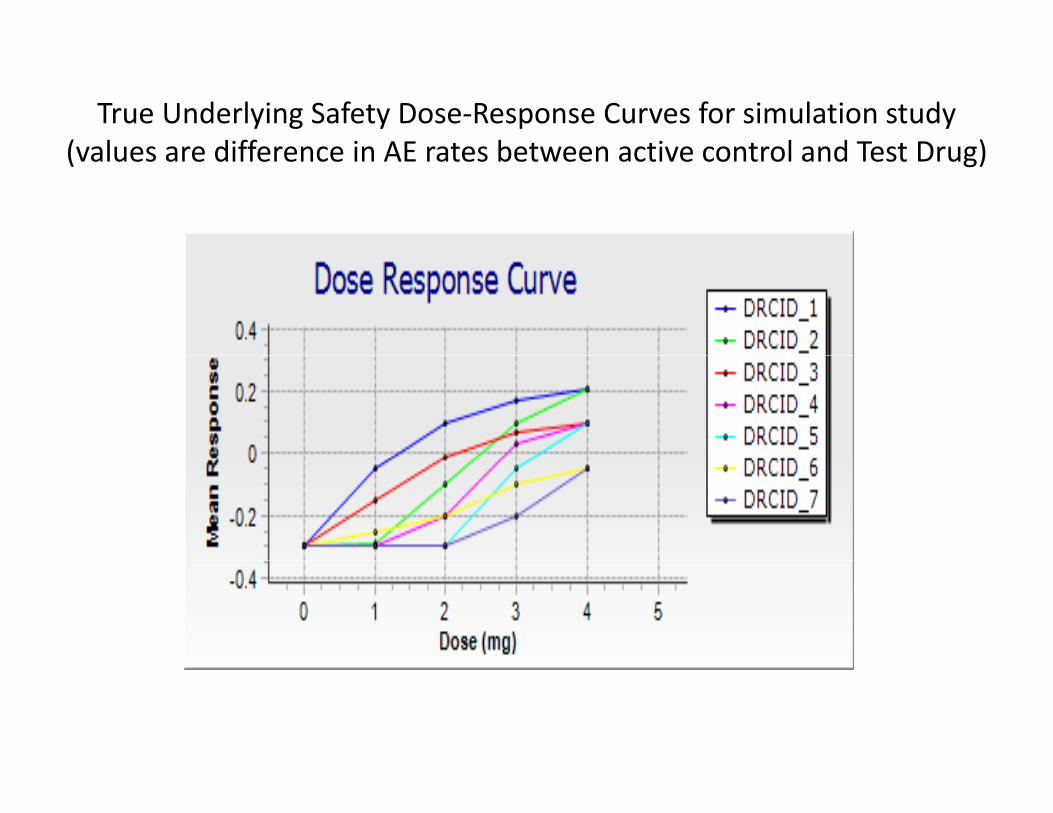
True Underlying Safety Dose‐Response Curves for simulation study (values are difference in AE rates between active control and Test Drug)(values are difference in AE rates between active control and Test Drug)
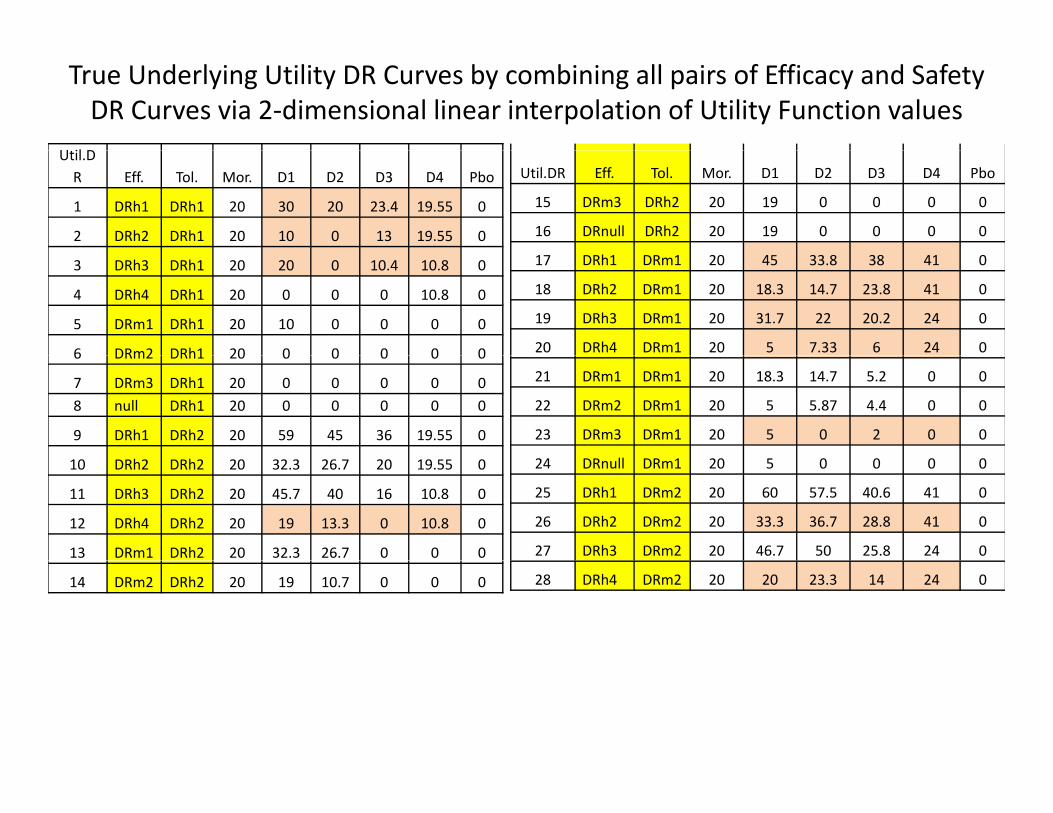
True Underlying Utility DR Curves by combining all pairs of Efficacy and Safety DR Curves via 2‐dimensional linear interpolation of Utility Function values
U il DUtil.DR Eff. Tol. Mor. D1 D2 D3 D4 Pbo
1 DRh1 DRh1 20 30 20 23.4 19.55 0
2 DRh2 DRh1 20 10 0 13 19.55 0
Util.DR Eff. Tol. Mor. D1 D2 D3 D4 Pbo
15 DRm3 DRh2 20 19 0 0 0 0
16 DRnull DRh2 20 19 0 0 0 0
3 DRh3 DRh1 20 20 0 10.4 10.8 0
4 DRh4 DRh1 20 0 0 0 10.8 0
5 DRm1 DRh1 20 10 0 0 0 0
6 DRm2 DRh1 20 0 0 0 0 0
17 DRh1 DRm1 20 45 33.8 38 41 0
18 DRh2 DRm1 20 18.3 14.7 23.8 41 0
19 DRh3 DRm1 20 31.7 22 20.2 24 0
20 DRh4 DRm1 20 5 7.33 6 24 06 DRm2 DRh1 20 0 0 0 0 0
7 DRm3 DRh1 20 0 0 0 0 08 null DRh1 20 0 0 0 0 0
9 DRh1 DRh2 20 59 45 36 19.55 0
21 DRm1 DRm1 20 18.3 14.7 5.2 0 0
22 DRm2 DRm1 20 5 5.87 4.4 0 0
23 DRm3 DRm1 20 5 0 2 0 0
ll10 DRh2 DRh2 20 32.3 26.7 20 19.55 0
11 DRh3 DRh2 20 45.7 40 16 10.8 0
12 DRh4 DRh2 20 19 13.3 0 10.8 0
13 DRm1 DRh2 20 32.3 26.7 0 0 0
24 DRnull DRm1 20 5 0 0 0 0
25 DRh1 DRm2 20 60 57.5 40.6 41 0
26 DRh2 DRm2 20 33.3 36.7 28.8 41 0
27 DRh3 DRm2 20 46.7 50 25.8 24 0
14 DRm2 DRh2 20 19 10.7 0 0 0 28 DRh4 DRm2 20 20 23.3 14 24 0

True Underlying Utility DR Curves by combining all pairs of Efficacy and Safety DR Curves via 2‐dimensional linear interpolation of Utility Function values
Util.DR Eff. Tol. Acntl D1 D2 D3 D4 Pbo
29 DRm1 DRm2 20 33.3 36.7 12.1 0 0
30 DRm2 DRm2 20 20 20.7 10.3 0 0
Util.DR Eff. Tol. Acntl D1 D2 D3 D4 Pbo
43 DRh3 DRl1 20 41.7 50 44 40.5 0
44 DRh4 DRl1 20 15 23.3 40 40.5 0
l31 DRm3 DRm2 20 20 10 4.67 0 0
32 DRnull DRm2 20 20 10 0 0 0
33 DRh1 DRm3 20 60 70 45.8 41 0
45 DRm1 DRl1 20 28.3 36.7 34.7 30 0
46 DRm2 DRl1 20 15 20.7 29.3 30 0
47 DRm3 DRl1 20 15 10 13.3 30 0
48 DR ll DRl1 20 15 10 0 0 034 DRh2 DRm3 20 33.3 46.7 38.8 41 0
35 DRh3 DRm3 20 46.7 60 37 24 0
36 DRh4 DRm3 20 20 33.3 30 24 0
48 DRnull DRl1 20 15 10 0 0 0
49 DRh1 DRl2 20 60 70 63.5 50.75 0
50 DRh2 DRl2 20 33.3 46.7 57.5 50.75 0
51 DRh3 DRl2 20 46.7 60 56 40.5 037 DRm1 DRm3 20 33.3 46.7 26 0 0
38 DRm2 DRm3 20 20 30.7 22 0 0
39 DRm3 DRm3 20 20 20 10 0 0
52 DRh4 DRl2 20 20 33.3 50 40.5 0
53 DRm1 DRl2 20 33.3 46.7 44.7 30 0
54 DRm2 DRl2 20 20 30.7 39.3 30 0
l40 DRnull DRm3 20 20 20 0 0 041 DRh1 DRl1 20 55 57.5 49 50.75 042 DRh2 DRl1 20 28.3 36.7 45 50.75 0
55 DRm3 DRl2 20 20 20 23.3 30 0
56 DRnull DRl2 20 20 20 10 0 0

True underlying utility functions for the simulation study(yellow highlighted value is maximum utility value for indicated DR curve
Representative set of utility DR curves to simulate
DR Curve pbo D1 D2 D3 D41 0 0 0 0 111 0 0 0 0 112 0 10 0 0 03 0 32 27 20 204 0 46 40 16 115 0 60 58 41 416 0 20 21 10 07 0 20 10 5 08 0 20 33 30 249 0 55 58 50 5010 0 28 37 45 5111 0 15 23 40 4112 0 20 33 50 4112 0 20 33 50 4113 0 20 31 39 3014 0 20 20 23 30

True underlying utility functions for h l dthe simulation study

Simulation Specifications• Stage A N=25 on pbo 4 doses Test Drug active control• Stage A N=25 on pbo, 4 doses Test Drug, active control
– Pause enrolment for Stage B starting dose selection• Stage B 10 cohorts N=25, maximizing design adaptationStage B 10 cohorts N 25, maximizing design adaptation
beginning with 4th Stage B cohort• Simulated 1000 times for each of 14 selected utility functions
– Normally distributed means per utility function– Conservatively assumed SD of a 0‐100 uniform distributionNO t ti t 0 100 l i t b ti i– NO truncation to 0‐100 scale – again to be conservative in order to preserve the assumed SD
– Therefore, actual design performance may be even betterTherefore, actual design performance may be even better than reported herein.
• Custom SAS program

Performance Characteristics Computed1000 i l ti h f 14 tilit DRacross 1000 simulations per each of 14 utility DR curves
• Average estimated target doseg g• Proportion of simulations in which the correct target dose was
estimated• Proportion of simulations in which the estimated target dose
was adjacent to the correct target dose• Average number of subjects assigned to each doseAverage number of subjects assigned to each dose
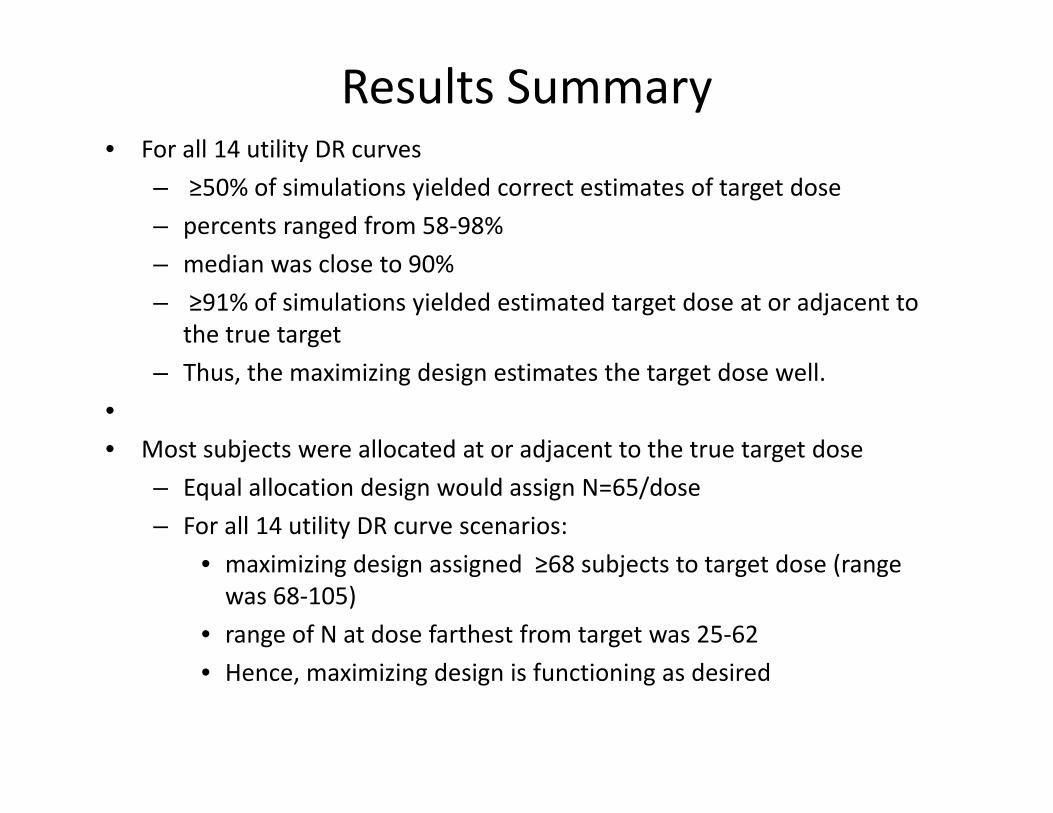
Results Summary• For all 14 utility DR curves• For all 14 utility DR curves
– ≥50% of simulations yielded correct estimates of target dose– percents ranged from 58‐98%– median was close to 90%– ≥91% of simulations yielded estimated target dose at or adjacent to
the true target– Thus, the maximizing design estimates the target dose well.
•• Most subjects were allocated at or adjacent to the true target dosej j g
– Equal allocation design would assign N=65/dose– For all 14 utility DR curve scenarios:
• maximizing design assigned ≥68 subjects to target dose (range• maximizing design assigned ≥68 subjects to target dose (range was 68‐105)
• range of N at dose farthest from target was 25‐62d f d d• Hence, maximizing design is functioning as desired

Performance characteristics of maximizing design (N=400)based on 1000 simulations of each utility DR curveT E ti t d % ti ti % ti ti % ti ti t
DR#
True Target Dose
Estimated Target Dose Average
% estimating exactly at True Target Dose
% estimating adjacent to True Target Dose
% estimating at or adjacent to True Target Dose
1 4 3.9 93 1 952 1 1.3 87 4 913 1 1.3 77 21 984 1 1.1 86 14 1005 1 1.4 58 42 1006 2 1.6 64 36 1007 1 1.0 96 3 998 2 2.3 74 25 989 2 1 9 72 24 969 2 1.9 72 24 9610 4 3.9 91 9 10011 4 3.6 59 41 10012 3 3 0 98 2 10012 3 3.0 98 2 10013 3 3.0 93 7 10014 4 3.7 86 6 92

Average N’s assigned to each dose across 1000 simulations for each utility DR curve
(yellow highlighted cells indicate TRUE target dose)(yellow highlighted cells indicate TRUE target dose)Average Number of Subjects Assigned to Each Dose
DR# D1 D2 D3 D41 30 32 100 982 86 91 44 393 82 89 48 414 91 97 39 335 73 82 57 486 68 87 62 437 98 101 32 298 41 71 89 599 53 68 77 629 53 68 77 6210 25 33 105 9711 25 45 105 8512 25 63 105 6712 25 63 105 6713 28 64 102 6614 31 37 99 93

Overall Summary• Phase 2 trial of Test Drug versus placebo and active control• Phase 2 trial of Test Drug versus placebo and active control• Objectives: PoC + estimate dose regimen with optimal balance between
maximum efficacy and minimum intolerance• Maximizing adaptive dose‐finding design (Ivanova, 2009) chosen to yield g p g g ( ) y
better quality information– fewer patients assigned to dose regimens which are ineffective or
intolerable• True potential efficacy and tolerability dose response (DR) curves were• True potential efficacy and tolerability dose‐response (DR) curves were
constructed to span the range of potential DR curves for Test Drug• Clinical utility function defined to combine all of the efficacy and
tolerability dose‐response curves• Simulation study evaluated performance characteristics• Results indicate the maximizing design
– Has high probability to estimate the correct or nearest to correct dose with maximum clinical utility (i e “target dose”)with maximum clinical utility (i.e., target dose )
– Maximizes assignment of subjects to the target dose– Minimizes assignment of subject to doses remote from target dose

Case Study 2Adaptive Dose‐Finding Designp g g
for 2‐drug Combination
Jim Bolognese, CytelEAST UGM22Oct201422Oct2014

Assumptions for Adaptive Design
K E d i t 0 3 i t Lik t S l Gl b l A t f R t• Key Endpoint: 0‐3 point Likert Scale Global Assessment of Response to Therapy (0=none; 1=some; 2=good; 3=excellent)– Since sample size is “large”, can use continuous endpoint stat methods
(i l di t ib ti )(i.e., assume normal distribution)• Typical for global assessments of response to therapy in arthritis and pain using Likert scale responses similar to above
– Prior data: mean difference between active & placebo 2.2 vs 1.6 (SD~0.9)• Suggests N=41/treatment group for 80% power (alpha=0.05, 1‐sided)
• Traditional Design would have 2 or 3 dose‐combinations plus placebo (N=123 to 164)
• Investigate Adaptive Dose‐finding Phase 2 trial design with Total N=135– 3 doses of 1st drug + 3 doses of 2nd drug (9 dose‐combinations) + placebo3 doses of 1 drug 3 doses of 2 drug (9 dose combinations) placebo– Ivanova(2012) Bayesian Isotonic 2‐dimensional design software (CytelSim
– in‐house tool) updated to accommodate 3x3 dose‐combinations

Overview of Adaptive Design
I iti l C h t N 46 (10 36 l b d 4/d bi ti )• Initial Cohort N=46 (10:36, placebo:drug, 4/dose‐combination)• 3 additional cohorts, each N=30 (7:23 pbo:drug), with doses assigned
adaptively• Extension of Adaptive Dose‐Finding Design (Ivanova, 2012)
– Optimizes dose‐assignments for Target Responses 0.5 and 1.0 (arbitrarily chosen, can be modified) different from placebo
– Assumes non‐decreasing response with increasing dose of each drug within each dose‐level of the other drug
– Models the dose‐response relationship via isotonic regression• Improves statistical efficiency compared to raw means
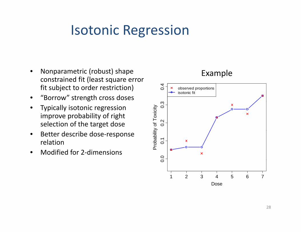
Isotonic Regression
• Nonparametric (robust) shape ExampleNonparametric (robust) shape constrained fit (least square error fit subject to order restriction)
• “Borrow” strength cross doses
0.4
observed proportionsisotonic fit
Example
• Typically isotonic regression improve probability of right selection of the target dose 0.
20.
3ty
of T
oxic
ity
• Better describe dose‐response relation
• Modified for 2‐dimensions0.
00.
1Pr
obab
ilit
1 2 3 4 5 6 7
0
Dose
28
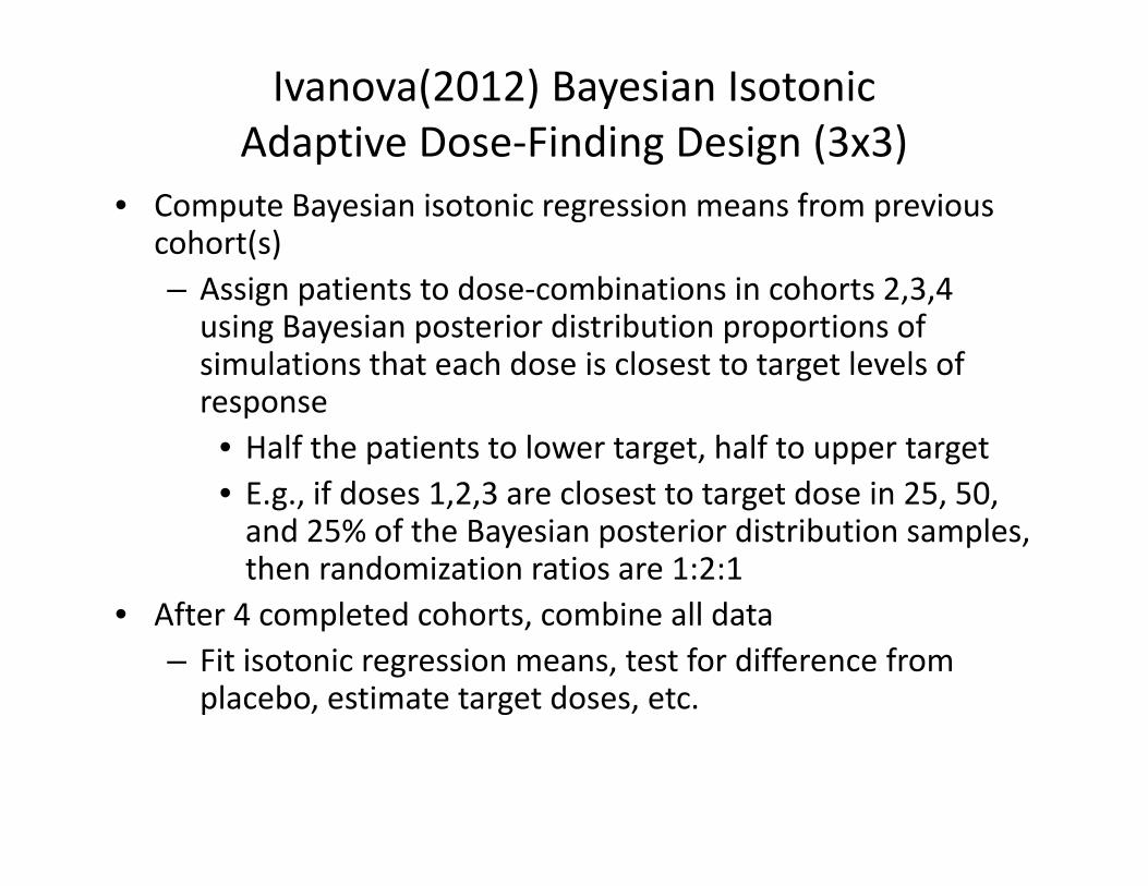
Ivanova(2012) Bayesian Isotonic Adaptive Dose‐Finding Design (3x3)p g g ( )
• Compute Bayesian isotonic regression means from previous cohort(s)– Assign patients to dose‐combinations in cohorts 2,3,4 using Bayesian posterior distribution proportions of simulations that each dose is closest to target levels of response
• Half the patients to lower target, half to upper target• E g if doses 1 2 3 are closest to target dose in 25 50E.g., if doses 1,2,3 are closest to target dose in 25, 50, and 25% of the Bayesian posterior distribution samples, then randomization ratios are 1:2:1
• After 4 completed cohorts combine all data• After 4 completed cohorts, combine all data– Fit isotonic regression means, test for difference from placebo, estimate target doses, etc.

Assess usefulness of Adaptive Dose‐Finding Design: Compare Performance Characteristics
Si l i l f h f h 2 i l d• Simulation results for each of the 2 potential dose‐response scenarios are summarized by the following performance characteristics, compared between adaptive and traditional non‐adaptive designs:– Power to yield statistically significant (alpha=0.05, 1‐sided) difference from placebodifference from placebo
– Average assigned sample size per dose– Probability of identifying the correct target doseProbability of identifying the correct target dose
• Multiple dose‐response scenarios chosen as examples of TRUE underlying DR curves to assess performance characteristics

Assumed True Underlying Dose‐Response Curvesfor Simulations
• “R” designates one drug• “d” designates 2nd drug "good" response (SD=0.9)
b 1 6 d1 d2 d3• R0d0 is placebo• R2d3 designates 2nd highest dose
of Drug R, 3rd highest dose of
pbo=1.6 d1 d2 d3R1 1.6 2.1 2.3R2 1.8 2.3 2.4g , g
Drug d, etc.• Pink Highlighted Cells indicate
doses with Target Levels of
R3 2.1 2.3 2.6
"zero" response (SD=0.9)gResponse (0.5 or 1.0 different from placebo)
zero response (SD 0.9)pbo=1.6 d1 d2 d3
R1 1.6 1.6 1.6R2 1 6 1 6 1 6R2 1.6 1.6 1.6R3 1.6 1.6 1.6

Additional Assumed True Underlying Dose‐Response Curves (Pink Highlighted Cells indicate doses with Target Levels of Response: 0.5 or 1.0
different from placebo)different from placebo)
“decreasing DR” (SD=0.9)pbo=1.6 D1 d2 D3
“constant2.1” (SD=0.9)pbo=1.6 d1 d2 d3
R1 2.6 2.35 2.1
R2 2.35 2.1 1.85
R3 2 1 1 85 1 6
R1 2.1 2.1 2.1
R2 2.1 2.1 2.1
R3 2 1 2 1 2 1 R3 2.1 1.85 1.6
“U‐shaped DR” (SD=0.9)
R3 2.1 2.1 2.1
“constant2.6” (SD=0.9)pbo=1.6 D1 d2 d3
R1 1.6 1.85 2.1
R2 1.85 2.6 1.85
pbo=1.6 d1 d2 d3R1 2.6 2.6 2.6
R2 2.6 2.6 2.6
R3 2.1 1.85 1.6R3 2.6 2.6 2.6

Additional Assumed True Underlying Dose‐Response Curves (Pink Highlighted Cells indicate doses with Target Levels of Response: 0.5 or 1.0
different from placebo)
“linear low DR” (SD=0.9)pbo=1.6 D1 d2 d3
“linear DR” (SD=0.9)pbo=1.6 d1 d2 d3
different from placebo)
R1 1.6 1.7 1.8
R2 1.7 1.8 2.1
R3 1 8 2 1 2 6
R1 1.6 1.85 2.1
R2 1.85 2.1 2.35
R3 2 1 2 35 2 6 R3 1.8 2.1 2.6
“asymmetric DR” (SD=0.9)
R3 2.1 2.35 2.6
“linear plateau DR” (SD=0.9)pbo=1.6 d1 d2 D3
R1 1.85 2.0 2.5
R2 1.9 2.1 2.6
pbo=1.6 d1 d2 d3R1 1.8 2.1 2.6
R2 2.1 2.6 2.6
R3 1.9 2.1 2.6R3 2.6 2.6 2.6

Additional Assumed True Underlying Dose‐Response Curves (Pink Highlighted Cells indicate doses with Target Levels of Response: 0.5 or 1.0
different from placebo)
Only 1active2.6 (SD=0.9)pbo=1.6 d1 d2 d3
Step Function (SD=0.9)pbo=1.6 d1 d2 d3
different from placebo)
R1 1.6 1.6 1.6
R2 2.2 2.2 2.2
R3 2 6 2 6 2 6
R1 1.6 1.6 1.6
R2 1.6 1.6 2.6
R3 1 6 2 6 2 6 R3 2.6 2.6 2.6
DR4 (SD=0.9)
R3 1.6 2.6 2.6
Only1 active2.8 (SD=0.9)pbo=1.6 d1 d2 d3
R1R2
pbo=1.6 d1 d2 d3R1 1.6 1.6 1.6
R2 2.2 2.2 2.2
R3R3 2.8 2.8 2.8

Assumed True Underlying Dose‐Response Curvesfor Simulations
• “R” designates one drug; “d” designates 2nd drug; R0d0 is placebo• R2d3 designates middle dose (2) of Drug R, highest dose (3) of Drug d• Pink Highlighted Cells indicate doses with Target Levels of Response (0 5 orPink Highlighted Cells indicate doses with Target Levels of Response (0.5 or
1.0 different from placebo)
3x3 format3x3 formatpbo=1.6 d1 d2 d3
R1 1.6 2.1 2.3R2 1 8 2 3 2 4R2 1.8 2.3 2.4R3 2.1 2.3 2.6
Linear Format R0d0 R1d1 R1d2 R1d3 R2d1 R2d2 R2d3 R3d1 R3d2 R3d3Increasing DR 1.6 1.6 2.1 2.3 1.8 2.3 2.4 2.1 2.3 2.6g

Assumed True Underlying Dose‐Response Curvesfor Simulations
• “R” designates one drug; “d” designates 2nd drug; R0d0 is placebo• R2d3 designates middle dose (2) of Drug R, highest dose (3) of Drug d• Pink Highlighted Cells indicate doses with Target Levels of Response (0 5 orPink Highlighted Cells indicate doses with Target Levels of Response (0.5 or
1.0 different from placebo)R0d0 R1d1 R1d2 R1d3 R2d1 R2d2 R2d3 R3d1 R3d2 R3d3
increasing 1.6 1.6 2.1 2.3 1.8 2.3 2.4 2.1 2.3 2.6increasing 1.6 1.6 2.1 2.3 1.8 2.3 2.4 2.1 2.3 2.6all2.1 1.6 2.1 2.1 2.1 2.1 2.1 2.1 2.1 2.1 2.1all2.6 1.6 2.6 2.6 2.6 2.6 2.6 2.6 2.6 2.6 2.6
null 1 6 1 6 1 6 1 6 1 6 1 6 1 6 1 6 1 6 1 6null 1.6 1.6 1.6 1.6 1.6 1.6 1.6 1.6 1.6 1.6
decreasing DR 1.6 2.6 2.35 2.1 2.35 2.1 1.85 2.1 1.85 1.6u-shaped DR 1.6 1.6 1.85 2.1 1.85 2.6 1.85 2.1 1.85 1.6
linear DR 1.6 1.6 1.85 2.1 1.85 2.1 2.35 2.1 2.35 2.6linear low DR 1.6 1.6 1.7 1.8 1.7 1.8 2.1 1.8 2.1 2.6linear plateau 1.6 1.8 2.1 2.6 2.1 2.6 2.6 2.6 2.6 2.6
DRasymmetric DR 1.6 1.85 2 2.5 1.9 2.1 2.6 1.9 2.1 2.6
Step Function 1.6 1.6 1.6 1.6 1.6 1.6 2.6 1.6 2.6 2.6

Number of patients assigned to each dose‐combinationAverage N per Dose‐Combination Group
TRUE DR Curve R0d0 R1d1 R1d2 R1d3 R2d1 R2d2 R2d3 R3d1 R3d2 R3d3increasing 31 10 13 13 11 11 11 12 12 13
all2.1 31 13 10 11 9 9 10 10 10 22all2.6 31 24 11 10 11 9 9 10 9 12
null 31 8 8 10 8 8 11 9 10 33decreasing DR 31 16 8 9 8 8 9 8 8 29decreasing DR 31 16 8 9 8 8 9 8 8 29
u-shaped DR 31 9 11 11 10 10 9 9 8 27linear DR 31 10 11 13 10 11 12 12 12 14
linear low DR 31 9 9 12 9 11 14 11 15 16Lin.plateauDR 31 13 14 13 13 11 9 11 9 11asymmetricDR 31 11 11 14 10 11 11 11 13 14
With this sample size, algorithm allocates fewer patients away from doses with target levels of response
asymmetricDR 31 11 11 14 10 11 11 11 13 14Step Function 31 8 9 13 9 13 15 13 14 11
levels of responseIn some cases, the isotonic smoothing results in increased allocation at some of the higher dose combinationsIn general, dose‐assignments are improved from equal allocation

Number of patients assigned to each dose‐combinationAverage N per Dose‐Combination Group
TRUE DR Curve R0d0 R1d1 R1d2 R1d3 R2d1 R2d2 R2d3 R3d1 R3d2 R3d3increasing 31 10 13 13 11 11 11 12 12 13
all2.1 31 13 10 11 9 9 10 10 10 22all2.6 31 24 11 10 11 9 9 10 9 12
null 31 8 8 10 8 8 11 9 10 33Only 1active2 6 31 9 9 13 13 12 13 13 10 12Only 1active2.6 31 9 9 13 13 12 13 13 10 12Only 1active2.8 31 9 10 13 14 12 15 13 9 10
linear DR 31 10 11 13 10 11 12 12 12 14linear low DR 31 9 9 12 9 11 14 11 15 16Lin.plateauDR 31 13 14 13 13 11 9 11 9 11asymmetricDR 31 11 11 14 10 11 11 11 13 14
With this sample size, algorithm allocates fewer patients away from doses with target levels of response
asymmetricDR 31 11 11 14 10 11 11 11 13 14Step Function 31 8 9 13 9 13 15 13 14 11
levels of responseIn some cases, the isotonic smoothing results in increased allocation at some of the higher dose combinationsIn general, dose‐assignments are improved from equal allocation

Performance CharacteristicsPower(%)
% at lower TGT*
%at/near lower TGT
% at upper TGT
% at/near upper TGT(%) lower TGT* lower TGT upper TGT upper TGT
increasing 79 50 1 38 84all2.1 66 19 47 92 98all2 6 98 94 99 23 44all2.6 98 94 99 23 44
null 5.0 93 98 99 100decreasing DR 21 24 100 04 13
h d DR 8 20 60 4 100u-shaped DR 8 20 60 4 100linear DR 78 65 100 41 93
linear low DR 74 48 95 61 99linear plateau DR 77 74 100 95 100
asymmetric DR 79 40 100 61 99Step Function 66 86 100 98 100
• Relatively high power for the monotonic dose‐response configurations
p 66 86 00 98 00* TGT = lowest dose combination with target level of response
• Moderate‐to‐high probability of estimating correct dose‐combination• Very low probability of identifying dose‐combination NOT at or near Target

Performance CharacteristicsPower(%)
% at lower TGT*
%at/near lower TGT
% at upper TGT
% at/near upper TGT(%) lower TGT* lower TGT upper TGT upper TGT
increasing 79 50 1 38 84all2.1 66 19 47 92 98all2 6 98 94 99 23 44all2.6 98 94 99 23 44
null 5.0 93 98 99 100Only 1active2.6 73 74 100 72 100Only 1active2.8 72 76 100 57 100
linear DR 78 65 100 41 93linear low DR 74 48 95 61 99
linear plateau DR 77 74 100 95 100asymmetric DR 79 40 100 61 99
Step Function 66 86 100 98 100
• Relatively high power for the monotonic dose‐response configurations
Step Function 66 86 100 98 100* TGT = lowest dose combination with target level of response
• Moderate‐to‐high probability of estimating correct dose‐combination• Very low probability of identifying dose‐combination NOT at or near Target
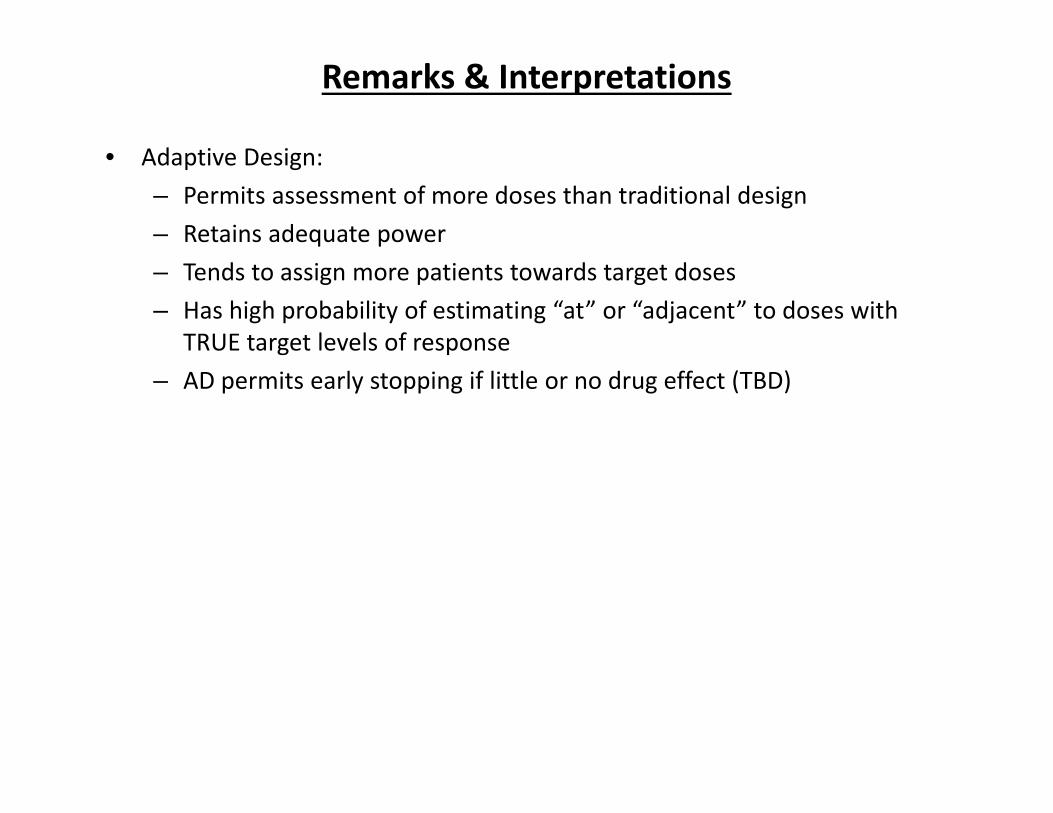
Remarks & Interpretations
Ad ti D i• Adaptive Design:– Permits assessment of more doses than traditional design– Retains adequate power– Tends to assign more patients towards target doses– Has high probability of estimating “at” or “adjacent” to doses with
TRUE target levels of response– AD permits early stopping if little or no drug effect (TBD)
Next Steps
• Identify design logistics (Enrolment rate, timing of end point observation, y g g ( , g p ,cohort sizes, number of adaptations, early stopping rules, other??)– To be addressed in draft protocol synopsis needed by end of summer
• Additional simulations to assess design improvements (after review of aboveAdditional simulations to assess design improvements (after review of above simulation summary):– size of initial cohort
total sample size– total sample size– early stopping for futility

C S d 3Case Study 3Adaptive Phase 2 Dose‐Finding Design
for Proof‐of‐Concept & Dose‐Explorationvia Linear Clinical Utility Function
Jim Bolognese, Cytel Inc.EAST UGM22Oct201422Oct2014
43

OUTLINEOUTLINE
• Adaptive design based on linear function ofAdaptive design based on linear function of efficacy + tolerability for clinical utility
• Simulation results of two design choices• Simulation results of two design choices document performance characteristics of each designdesign
44

Overall Summary• Phase 2 trial of test drug versus placebog p• Objectives: PoC + estimate dose regimen with optimal balance between
maximum efficacy and minimum intolerance• Maximizing adaptive dose‐finding design yields better quality informationMaximizing adaptive dose finding design yields better quality information
– fewer patients assigned to dose regimens which are ineffective or intolerable
– IVANOVA (2009)IVANOVA (2009)– Normal Dynamic Linear Model (NDLM, COMPASS User Manual, Cytel Inc.)
• True potential efficacy and tolerability dose‐response (DR) curves were constructed to span the range of potential DR curvesconstructed to span the range of potential DR curves
• Linear clinical utility function combines efficacy and tolerability dose‐response curves
• Simulation study evaluated performance characteristics• Simulation study evaluated performance characteristics• Results indicate the maximizing design
– Has high probability to estimate the correct or nearest to correct dose ith i li i l tilit (i “t t d ”)with maximum clinical utility (i.e., “target dose”)
– Maximizes assignment of subjects at or adjacent to the target dose– Minimizes assignment of subject to doses remote from target dose 45

Clinical Utility Function DefinitionCU ( ffi l b ) (BP ff t l b )• CU = (efficacy vs placebo) – (BP effect vs placebo)– Efficacy target difference from placebo = 4– BP target difference from placebo < 10mmHg– CU = w1*(EFF drug – EFF placebo)*(10/4)
– w2*(∆BP drug – ∆BP placebo)• Where w1=1.5 and w2=1, i.e., Efficacy effect is weighted 50% moreWhere w1 1.5 and w2 1, i.e., Efficacy effect is weighted 50% more than BP effect
– Examples• 1 5*(4 – 4)*(10/4) – (10 –10) = 0• 1.5 (4 – 4) (10/4) – (10 –10) = 0• 1.5*(4 – 4)*(10/4) – (10 –0) = ‐10• 1.5*(4 – 0)*(10/4) – (10 –10) = +15• 1.5*(4 – 0)*(10/4) – (10 –0) = +5
– Refer to accompanying spreadsheet for more detail and more examples
46

Efficacy and Tolerability TRUE DR CurvesEfficacy response
scenario placebo dose1 dose2 dose3 dose4 dose51:null 0 0 0 0 0 02:modest 0 0 1 2 3 43 d t 0 1 2 4 5 53:moderate 0 1 2 4 5 54:robust 0 1 4 5 5 5
BP response1:null 0 0 0 0 0 01:null 0 0 0 0 0 02:modest 0 0 5 10 15 203:moderate 0 5 10 20 30 40
47
3:moderate 0 5 10 20 30 404:robust 0 5 20 30 40 50

TRUE Clinical Utility DR Curves (SD=38)Scenario Combination Clinical Utility Values*Efficacy BP placebo dose1 dose2 dose3 dose4 dose51:null 1:null 0 0 0 0 0 01:null 2:modest 0 0 ‐5 ‐10 ‐15 ‐201:null 3:moderate 0 ‐5 ‐10 ‐20 ‐30 ‐401:null 3:moderate 0 ‐5 ‐10 ‐20 ‐30 ‐401:null 4:robust 0 ‐5 ‐20 ‐30 ‐40 ‐50
2:modest 1:null 0 0 3.75 7.5 11.25 152:modest 2:modest 0 0 ‐1.25 ‐2.5 ‐3.75 ‐52:modest 3:moderate 0 ‐5 ‐6.25 ‐12.5 ‐18.75 ‐252:modest 4:robust 0 ‐5 ‐16.25 ‐22.5 ‐28.75 ‐35
3:moderate 1:null 0 3.75 7.5 15 18.75 18.753:moderate 2:modest 0 3.75 2.5 5 3.75 ‐1.253:moderate 3:moderate 0 ‐1 25 ‐2 5 ‐5 ‐11 25 ‐21 253:moderate 3:moderate 0 ‐1.25 ‐2.5 ‐5 ‐11.25 ‐21.253:moderate 4:robust 0 ‐1.25 ‐12.5 ‐15 ‐21.25 ‐31.25
4:robust 1:null 0 3.75 15 18.75 18.75 18.75
48
4:robust 2:modest 0 3.75 10 8.75 3.75 ‐1.254:robust 3:moderate 0 ‐1.25 5 ‐1.25 ‐11.25 ‐21.254:robust 4:robust 0 ‐1.25 ‐5 ‐11.25 ‐21.25 ‐31.25

Assumptions for Adaptive Design for Clinical Utility
5 d f d (4 8 12 16 20 ) l l b• 5 doses of test drug (4,8,12,16,20mg) plus placebo– Total N=192
• 1st cohort N=24 (4:4:4:4:4:4)• 1 cohort N=24 (4:4:4:4:4:4)• 10 cohorts N=14, 7 on each of 2 doses adaptively assigned per maximizing design
– Adaptive Design permits early stopping for futility if Conditional Power < 10% after 1st 60 patients; not considered in initial simulationsin initial simulations
• Response Lag 2 weeks to permit 1 week observation and 1 week for collection and analysis of data to feed adaptation– Assumed 13/week enrolment over ~15 weeks to achieve N=192
49

Results of Simulated Maximizing Adaptive Design to Id tif D ith O ti l Cli i l UtilitIdentify Dose with Optimal Clinical Utility
• In general, the adaptive design migrates the assignment of i dj h d i h i li i lpatients at or adjacent to the dose with maximum clinical
utility• The design with a 2‐week lag in response works reasonablyThe design with a 2 week lag in response works reasonably
well at total N=192 for many circumstances, but there are some clinical utility function scenarios for which it does not (see e g scenario #12)(see, e.g., scenario #12)
• Increasing the sample size to nearly double overcomes the deficiency in the 2‐week lag.y g
50

Average sample size assigned by the adaptive design to each dose group (NOTE: non‐adaptive design would assign
approximately 32 per dose group)approximately 32 per dose group)Scenario Combination average sample size assigned by adaptive design Efficacy BP pbo D1 D2 D3 D4 D51:null 1:null 30 32 32 31 30 361:null 1:null 30 32 32 31 30 361:null 2:modest 30 57 38 30 18 171:null 3:moderate 30 78 34 21 14 131:null 4:robust 30 111 21 11 9 8
2:modest 1:null 30 13 21 37 39 502:modest 2:modest 30 23 31 49 31 252:modest 3:moderate 30 37 36 40 25 212:modest 4:robust 30 82 34 23 12 102:modest 4:robust 30 82 34 23 12 103:moderate 1:null 30 9 11 17 33 893:moderate 2:modest 30 15 19 30 37 593:moderate 3:moderate 30 22 23 28 34 533:moderate 4:robust 30 68 31 23 18 184:robust 1:null 30 9 13 25 49 644:robust 2:modest 30 11 23 40 47 394:robust 3:moderate 30 15 28 38 43 36
51
4:robust 3:moderate 30 15 28 38 43 364:robust 4:robust 30 45 45 33 22 14
yellow highlighted cells indicate dose with TRUE underlying maximum clinical utility

performance characteristics: Adaptive vs. NON‐adaptive designNDLM Adaptive Design NON‐Adaptive Design
Scenario Combination TRUE target dose
Average Estimated Target Dose
Percent of Simulations Estimating: Average
Estimated Target Dose
Percent of Simulations Estimating:
Efficacy BP at Target at/near Tgt at Target at/near Tgtll ll1:null 1:null 12 11.6 18 50 11.9 16 28
1:null 2:modest 4 5.5 75 90 5.9 69 751:null 3:moderate 4 4.1 98 100 4.3 94 981:null 4:robust 4 4.0 100 100 4.0 100 100
2:modest 1:null 12 16.1 28 60 16.4 24 402:modest 2:modest 12 11.7 57 88 12.0 49 612:modest 3:moderate 12 8.3 29 57 8.8 29 382:modest 4:robust 4 4.1 97 100 4.2 96 1003:moderate 1:null 20 19.5 90 99 19.4 86 1003:moderate 2:modest 20 17.5 58 83 17.6 60 773:moderate 3:moderate 20 16.6 56 76 16.4 54 703:moderate 4:robust 4 4.7 90 95 5.0 85 904:robust 1:null 16 18.2 37 100 18.4 30 484:robust 2:modest 16 15.4 46 96 15.6 42 584:robust 3:moderate 16 14.7 40 87 14.8 38 534:robust 4:robust 4 7.7 38 77 7.7 38 46
52

performance characteristics: Adaptive vs. NON‐adaptive design----------Maximizing Design------ -------------NDLM Design-----------Est Est
utility true max pct pct pct max pct pct pctDR max utility correct est correct utility correct est correct
curve utility dose estimates adjacent adjacent dose estimates adjacent adjacent1 3(12) 2.7 23 42 65 2.9 18 32 502 1( 4) 2.1 36 31 67 1.4 75 14 903 1( 4) 1.8 52 28 80 1.0 98 2 1004 1( 4) 1.3 83 10 92 1.0 100 0 1005 5(20) 3.2 18 26 44 4.0 28 32 606 3(12) 2.7 44 37 81 2.9 57 30 887 3(12) 2.4 39 34 73 2.1 29 28 578 1( 4) 1.7 55 23 78 1.0 97 3 1009 5(20) 4.3 68 13 81 4.9 90 9 9910 5(20) 3.4 31 18 49 4.4 58 24 8311 5(20) 3.1 24 19 43 4.1 56 20 7612 1( 4) 2.0 46 27 73 1.2 90 5 9513 5(20) 3.9 31 44 75 4.5 37 63 10014 4(16) 3.2 40 35 75 3.8 46 50 9615 4(16) 3.0 36 31 67 3.7 40 47 8716 2( 8) 2.2 38 51 88 1.9 38 38 77
53

Average Sample Sizes Assigned: Adaptive vs. NON‐adaptive design
DR ---Maximizing Design---- correct ------NDLM Design---------DR Maximizing Design correct NDLM Designcurve D1 D2 D3 D4 D5 Dmax* dose Dmax* D1 D2 D3 D4 D5
1 11 17 25 63 47 25 3 31 32 32 31 30 362 19 27 29 53 36 19 1 57 57 38 30 18 173 27 34 25 46 31 27 1 78 78 34 21 14 133 27 34 25 46 31 27 1 78 78 34 21 14 134 50 56 17 24 16 50 1 111 111 21 11 9 85 6 12 26 68 50 50 5 50 13 21 37 39 506 10 20 33 60 40 33 3 49 23 31 49 31 257 12 22 31 58 40 31 3 40 37 36 40 25 218 32 41 26 39 25 32 1 82 82 34 23 12 109 5 7 15 73 63 63 5 89 9 11 17 33 8910 6 10 21 70 56 56 5 59 15 19 30 37 5910 6 10 21 70 56 56 5 59 15 19 30 37 5911 9 13 21 67 52 52 5 53 22 23 28 34 5312 21 27 23 53 38 21 1 68 68 31 23 18 1813 4 7 26 73 53 53 5 64 9 13 25 49 6414 6 12 32 68 45 68 4 47 11 23 40 47 3915 7 13 32 67 44 67 4 43 15 28 38 43 3616 16 25 33 55 34 25 2 45 45 45 33 22 14
BOLD underlined values indicate doses with TRUE MAX Clin.Utility
54
y*Dmax indicates N assigned to dose with maximum clinical utility

Overall Summary• Phase 2 trial of test drug versus placebog p• Objectives: PoC + estimate dose regimen with optimal balance between
maximum efficacy and minimum intolerance• Maximizing adaptive dose‐finding design yields better quality informationMaximizing adaptive dose finding design yields better quality information
– fewer patients assigned to dose regimens which are ineffective or intolerable
– IVANOVA (2009)IVANOVA (2009)– Normal Dynamic Linear Model (NDLM, COMPASS User Manual, Cytel Inc.)
• True potential efficacy and tolerability dose‐response (DR) curves were constructed to span the range of potential DR curvesconstructed to span the range of potential DR curves
• Linear clinical utility function combines efficacy and tolerability dose‐response curves
• Simulation study evaluated performance characteristics• Simulation study evaluated performance characteristics• Results indicate the maximizing design
– Has high probability to estimate the correct or nearest to correct dose ith i li i l tilit (i “t t d ”)with maximum clinical utility (i.e., “target dose”)
– Maximizes assignment of subjects at or adjacent to the target dose– Minimizes assignment of subject to doses remote from target dose 55

Remarks & Potential Next Steps for Consideration• Maximizing Design via NDLM seems viable• Additional simulations could be conducted to assess if further
improvements can be made to:M dif l t t t 4/ k & l t 3 k– Modify enrolment rate to 4/week & lag to 3 weeks
– Sample Size (size of initial cohort, total N)– Utility Function Refinement ??Utility Function Refinement ??
56
References
• Ivanova A, Liu K, Snyder E, Snavely D. An adaptive design for identifying the dose with the best efficacy/tolerability profile with application to a crossover dose finding study Statistwith application to a crossover dose‐finding study. Statist. Med. 2009; 28:2941‐2951
• COMPASS V1.1 Users Manual, Cytel Inc., Cambridge, MA 2012• Ivanova A, Xiao C, Tymofyeyev Y. Two‐stage designs for Phase
2 dose‐finding trials. Statist. Med. 2012; 31:2872–2881