Solvent structure improves docking predictionin lectin–carbohydrate complexes

Diego F Gauto3,4, Ariel A Petruk4, Carlos P Modenutti2,Juan I Blanco2,4, Santiago Di Lella2,5, and MarceloA Martí1,2,4

2Departamento de Química Biológica, Facultad de Ciencias Exactas yNaturales; 3Departamento de Química Inorgánica, Analítica y Química Física;4Instituto de Química de los Materiales, Medio Ambiente y Energía(INQUIMAE), CONICET; and 5Instituto de Química Biológica - CienciasExactas y Naturales UBA/CONICET, Ciudad Universitaria, Pabellón 2,Buenos Aires C1428EHA, Argentina

Received on August 6, 2012; revised on October 10, 2012; accepted onOctober 10, 2012

Recognition and complex formation between proteins andcarbohydrates is a key issue in many important biologicalprocesses. Determination of the three-dimensional struc-ture of such complexes is thus most relevant, but particu-larly challenging because of their usually low bindingaffinity. In silico docking methods have a long-standingtradition in predicting protein–ligand complexes, andallow a potentially fast exploration of a number of possibleprotein–carbohydrate complex structures. However, deter-mining which of these predicted complexes represents thecorrect structure is not always straightforward.In this work, we present a modification of the scoring

function provided by AutoDock4, a widely used dockingsoftware, on the basis of analysis of the solvent structureadjacent to the protein surface, as derived from moleculardynamics simulations, that allows the definition and char-acterization of regions with higher water occupancy thanthe bulk solvent, called water sites. They mimic the inter-action held between the carbohydrate –OH groups and theprotein. We used this information for an improved dockingmethod in relation to its capacity to correctly predict theprotein–carbohydrate complexes for a number of testedproteins, whose ligands range in size from mono- to tetra-saccharide. Our results show that the presented method sig-nificantly improves the docking predictions. The resultingsolvent-structure-biased docking protocol, therefore,appears as a powerful tool for the design and optimizationof development of glycomimetic drugs, while providing newinsights into protein–carbohydrate interactions. Moreover,the achieved improvement also underscores the relevance

of the solvent structure to the protein carbohydrate recog-nition process.

Keywords: AutoDock4 / carbohydrate / complex / docking /galectins / hydration site / lectin / proteins / saccharide / solventstructure / water site

Introduction

Formation of protein–ligand complexes is one of the mostfundamental processes in biochemistry. For a given protein,identifying with high precision which ligands should bebound—and which should not—is thus a crucial requisite forthe accomplishment of a variety of tasks such as enzyme ca-talysis, cell communication, signaling, adhesion and differen-tiation. In a more applied field, the rational design of new andmore effective drugs also depends on our knowledge aboutthe specific protein–ligand complexes that can be established(Drews 2000; Feinberg et al. 2011; Loging et al. 2012). Inthis context, determination of the atomic resolution structurefor any given protein–ligand complex is of fundamental rele-vance to understanding and characterizing its interactions,with a potential strong impact in both basic and applied bio-chemistry (Fadda and Woods 2010; Powlesland et al. 2010).In silico strategies for predicting the structure of a given

protein–ligand (or protein–protein) complex are usually re-ferred as docking methods (Taylor et al. 2002; Brooijmansand Kuntz 2003; Leach et al. 2006; Englebienne andMoitessier 2009). Widely used in the last decade, they arecurrently an essential part of many protein biochemical char-acterization studies, and rational drug design programs(Amzel 1998; Shoichet et al. 2002; Barril and Javier Luque2012). The potential and reliability of any docking methodlies in its capability to correctly predict the complex structure,and therefore the interactions held between the units, takingas the starting point the protein and ligand structures separate-ly. Nevertheless, given the approximations involved in the the-oretical developments employed, results are not alwayssuccessfully achieved (Taylor et al. 2002; Kerzmann et al.2006, 2008; Leach et al. 2006; Nurisso et al. 2008; Agostinoet al. 2009; Englebienne and Moitessier 2009; Seco et al.2009; Feliu and Oliva 2010).Currently, there are several docking software packages

available (Goodsell et al. 1996; Morris et al. 1996;Brooijmans and Kuntz 2003; Li et al. 2003), and althoughseveral works have compared different docking programs and

1To whom correspondence should be addressed: e-mail: marcelo@qi.fcen.uba.ar; dgauto@qi.fcen.uba.ar

Glycobiology vol. 23 no. 2 pp. 241–258, 2013doi:10.1093/glycob/cws147Advance Access publication on October 22, 2012

© The Author 2012. Published by Oxford University Press. All rights reserved. For permissions, please e-mail: journals.permissions@oup.com 241

by guest on May 10, 2013

pdf.highwire.org

Dow

nloaded from

versions(Agostino et al. 2009, 2011; Mishra et al. 2012), thereis still no clear best choice. In particular, for sugar docking,the work by Mishra et al. (2012) showed that AutoDock3 per-forms better than version 4, Vina and DOCK (Moustakaset al. 2006; Trott and Olson 2010), but still yields many falsepositives. (Mishra et al. 2012; Agostino et al. 2009) on theother hand, showed that Glide (Friesner et al. 2004) andAutoDock4 (Morris et al. 1998) performed better, but theresults were strongly dependent on the particular ligand recep-tor pair. In any case, one of the most popular, widely usedand more important free under the GNU General PublicLicense, docking programs is AutoDock4. The method com-bines a genetic algorithm (Morris et al. 1998) to explore pos-sible binding conformations of the ligand and an empiricalfunction, including electrostatic, hydrophobic and solvationeffects, to compute the ligand-binding free energy (ΔGB), thusranking the resulting complex structure predictions (Goodsellet al. 1996; Huey et al. 2007).During the ligand-binding process, significant solvent re-

organization is produced along the contact surface. Severalworks in this area have shown that this reorganization contri-butes to the ligand binding free energy (Li and Lazaridis2003, 2005; Abel et al. 2008; Michel et al. 2009a, b;Luccarelli et al. 2010). From a structural viewpoint, and as aresult of the interactions held between the protein and thesolvent, water molecules are not placed randomly on themacromolecule surface, but instead tend to occupy specificpositions and orientations. The latter results in a well-definedsolvent structure associated with the protein surface, character-ized by regions of highly ordered water molecules (Li andLazaridis 2003; Di Lella et al. 2007; Gauto et al. 2009). Thisis especially evident in regions such as protein-active sites orligand-binding regions (Young et al. 2007), and together withthe fact that displacing these ordered water molecules hasbeen shown to improve and correlate with the experimentallydetermined binding free energy (Abel et al. 2008; Michelet al. 2009b) underscores the relevance of such well-definedsolvent structure (Li and Lazaridis 2003, 2005; Young et al.2007; de Beer et al. 2010).Carbohydrate-binding proteins are a large and diverse group

of biomolecules that harbors enzymes as well as noncatalyticmembers. Lectins, for example, are multivalent carbohydrate-binding proteins present in all living organisms displaying awide variety of biological activities, including cell recognition,communication and cell growth (Varki et al. 1999; Crockeret al. 2007; Dam and Brewer 2010). Some of them, like thewell-known and thoroughly studied galectins, have also recent-ly emerged as key components for the development of drugtargets in several diseases, including cancer (Hirabayashi 2004;Leffler et al. 2004; Rabinovich 2005; Kadirvelraj et al. 2008;Di Lella et al. 2011; Echeverria and Amzel 2011; Guardiaet al. 2011). In this context, understanding protein–carbohydrateinteractions with atomic resolution (i.e. determining the struc-ture of the corresponding complexes) is of fundamental import-ance in basic and applied glycobiology (Feinberg et al. 2001;Balzarini 2007; Banerji et al. 2007; Agostino et al. 2009, 2010,2011,; Ernst and Magnani 2009; Taylor and Drickamer 2009;Feng et al. 2010; Frank and Schloissnig 2010; Woods andTessier 2010; von der Lieth et al. 2011). A common, but

usually overlooked, feature of carbohydrates is the fact thattheir polar –OH groups quite frequently bind to hydrophilicpatches of the protein surface, resulting in significant solventdisplacement and reorganization (Li and Lazaridis 2003, 2005;Di Lella et al. 2007; Kadirvelraj et al. 2008; Gauto et al. 2009;Frank and Schloissnig 2010; Gauto et al. 2011; Saraboji et al.2012). Water molecules and carbohydrate –OH groups canparticipate in similar hydrogen bond networks when establish-ing contacts with protein surfaces. This has been recentlyevidenced and characterized by our group and others forseveral carbohydrate-binding sites (CBS) of a diverse set ofproteins (Di Lella et al. 2007; Gauto et al. 2009, 2011; Sarabojiet al. 2012). Therefore, it is expected that the correspondingsolvent structure would prove useful for the in silico predictionof protein–carbohydrate complex structures, with higher accur-acy than conventional docking methods.As a prerequisite for further calculations, we need to

provide a simple methodology to analyze and characterize thementioned solvent structure. In principle, interactions betweenwater molecules and a protein can be thoroughly studied bymeans of molecular dynamics (MD) simulations in an explicitwater environment. However, specialized methodologies arerequired to estimate accurately the structural and thermo-dynamic properties of the surface-bound water molecules (Liand Lazaridis 2003, 2005; Di Lella et al. 2007; Gauto et al.2009). One of the most potent methods for achieving this taskis based on the inhomogeneous fluid solvation theory (IFST)as developed by Li and Lazaridis (Li and Lazaridis 2003,2005). Using this methodology, we were recently able toshow that solvent structure and dynamics at protein surfacesinvolved in carbohydrate-binding proteins are very differentfrom those of the bulk solvent, allowing the identificationof the so-called WS or hydration sites. A WS corresponds toa definite region in the space adjacent to the protein surface,where the probability of finding a water molecule is signifi-cantly higher than that observed in the bulk solvent. A furtherthermodynamic and structural characterization can beachieved employing the IFST (Lazaridis 1998a, b; Di Lellaet al. 2007; Gauto et al. 2009).In the present work, we used the information provided by

the identification and characterization of the WS in the CBSof several carbohydrate-binding proteins, to modify thescoring function of the docking program AutoDock4(Goodsell et al. 1996; Morris et al. 1996; Huey et al. 2007;Morris et al. 2009), in order to perform the in silico predictionof their corresponding protein–ligand complex structures.To test the performance of the presented implementation, wechose six protein–carbohydrate complexes with known crystalstructures, whose ligands range in size from mono- to tetra-saccharide (as depicted in Scheme 1).The systems are: The carbohydrate-binding domains of a

large multimodular sialidase from Clostridium perfringes,belonging to the carbohydrate-binding modules number 32 and40, from now on referred to as carbohydrate-binding module32 (CBM32) and carbohydrate-binding module 40 (CBM40).Both modules display a β-sandwich fold with a singlemonosaccharide-binding site that binds Gal (β-D-galactose)and sialic acid (α-D-N-acetylneuraminic acid), respectively(Scheme 1A and B) (Boraston et al. 2007). These type of

DF Gauto et al.

242

by guest on May 10, 2013

pdf.highwire.org

Dow

nloaded from

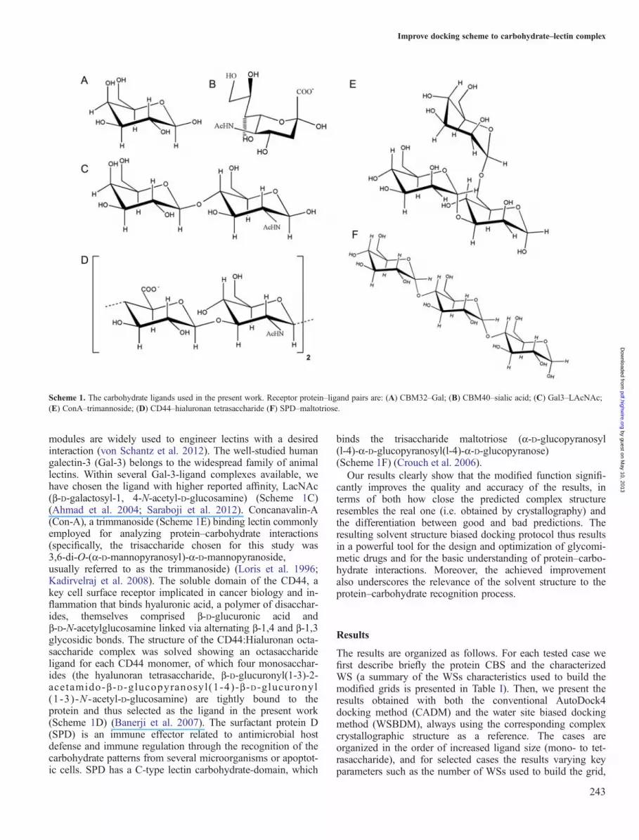
modules are widely used to engineer lectins with a desiredinteraction (von Schantz et al. 2012). The well-studied humangalectin-3 (Gal-3) belongs to the widespread family of animallectins. Within several Gal-3-ligand complexes available, wehave chosen the ligand with higher reported affinity, LacNAc(β-D-galactosyl-1, 4-N-acetyl-D-glucosamine) (Scheme 1C)(Ahmad et al. 2004; Saraboji et al. 2012). Concanavalin-A(Con-A), a trimmanoside (Scheme 1E) binding lectin commonlyemployed for analyzing protein–carbohydrate interactions(specifically, the trisaccharide chosen for this study was3,6-di-O-(α-D-mannopyranosyl)-α-D-mannopyranoside,usually referred to as the trimmanoside) (Loris et al. 1996;Kadirvelraj et al. 2008). The soluble domain of the CD44, akey cell surface receptor implicated in cancer biology and in-flammation that binds hyaluronic acid, a polymer of disacchar-ides, themselves comprised β-D-glucuronic acid andβ-D-N-acetylglucosamine linked via alternating β-1,4 and β-1,3glycosidic bonds. The structure of the CD44:Hialuronan octa-saccharide complex was solved showing an octasaccharideligand for each CD44 monomer, of which four monosacchar-ides (the hyalunoran tetrasaccharide, β-D-glucuronyl(1-3)-2-acetamido-β -D-glucopyranosyl(1-4)-β -D-glucuronyl(1-3)-N -acetyl-D-glucosamine) are tightly bound to theprotein and thus selected as the ligand in the present work(Scheme 1D) (Banerji et al. 2007). The surfactant protein D(SPD) is an immune effector related to antimicrobial hostdefense and immune regulation through the recognition of thecarbohydrate patterns from several microorganisms or apoptot-ic cells. SPD has a C-type lectin carbohydrate-domain, which

binds the trisaccharide maltotriose (α-D-glucopyranosyl(l-4)-α-D-glucopyranosyl(l-4)-α-D-glucopyranose)(Scheme 1F) (Crouch et al. 2006).Our results clearly show that the modified function signifi-

cantly improves the quality and accuracy of the results, interms of both how close the predicted complex structureresembles the real one (i.e. obtained by crystallography) andthe differentiation between good and bad predictions. Theresulting solvent structure biased docking protocol thus resultsin a powerful tool for the design and optimization of glycomi-metic drugs and for the basic understanding of protein–carbo-hydrate interactions. Moreover, the achieved improvementalso underscores the relevance of the solvent structure to theprotein–carbohydrate recognition process.

Results

The results are organized as follows. For each tested case wefirst describe briefly the protein CBS and the characterizedWS (a summary of the WSs characteristics used to build themodified grids is presented in Table I). Then, we present theresults obtained with both the conventional AutoDock4docking method (CADM) and the water site biased dockingmethod (WSBDM), always using the corresponding complexcrystallographic structure as a reference. The cases areorganized in the order of increased ligand size (mono- to tet-rasaccharide), and for selected cases the results varying keyparameters such as the number of WSs used to build the grid,

Scheme 1. The carbohydrate ligands used in the present work. Receptor protein–ligand pairs are: (A) CBM32–Gal; (B) CBM40–sialic acid; (C) Gal3–LAcNAc;(E) ConA–trimannoside; (D) CD44–hialuronan tetrasaccharide (F) SPD–maltotriose.

Improve docking scheme to carbohydrate–lectin complex

243

by guest on May 10, 2013

pdf.highwire.org

Dow

nloaded from

receptor structure and ligand size are presented and brieflydiscussed. At the beginning of the discussion, a final com-parative summary of all the obtained results is presented andthe results are analyzed.

Monosaccharide docking to CBM32 and CBM40 modulesWe begin our study by comparing the performance of theCADM and WSBDM for docking the lactose monosaccharideinto the CBS of the above described CBM32. This CBSharbors four WSs, as characterized in our previous work andshown in Table I, three of which (WS1, WS3 and WS4) aredisplaced by lactose upon binding. Figure 1 (left panel)shows the population vs. binding energy plots for lactosedocking to CBM32 crystal structure using the CADM. Theresults show that the method is incapable of correctly predict-ing the complex structure, since the lowest energy cluster isvery far from the reference structure. The highest Pop iscloser to the reference, but still clearly unacceptable(Figure 1C). Moreover, the docked configuration closest to thereference complex predicted structure has a root mean square

deviation (RMSD) of 2.9 Å and may be very difficult to iden-tify among other predictions.The results for the WSBDM using the four identified WSs

to build the grid are shown in Figure 1 right panel. Theresults are clearly better than those described above. Only twoclusters are found, which are very close in energy (differenceis only 0.2 kcal/mol, i.e. well below the method accuracy) andwith similar populations. However, the closest to the referencestructure, with only 1.1 Å RMSD, and therefore a very goodprediction as shown in Figure 1E, ranks second in both Popand ΔGB. The highest Pop predicted structure instead showsthe β-D-Gal slightly displaced and rotated ca. 60°, from thereference structure, as shown in Figure 1D. Similar results areobtained, when the receptor grid was built using a randomselected snapshot from the CBM32 ligand-free MD simula-tion (Supplementary data, Figure S1). Although for theWSBDM the correct structure still ranks second (and this timewith even lower population), it performs significantly betterthan the CADM.We now turn our attention to CBM40, presenting six well-

defined WS in its CBS region, as characterized in our previ-ous work and shown in Table I. The three sites with highestwater finding probability (WFP), WS1, WS3 and WS6 areall displaced by the ligand O8, C6 and the acid carboxylate,respectively. Figure 2 shows the population vs. bindingenergy plots for sialic acid docking to CBM40 crystal struc-ture using the CADM. The results show that the method ranksfirst the wrong complex structure (both in energy and popula-tion, with an RMSD of 4.7 Å compared with the reference),but correctly predicts the complex as the second best choice.The WSBDM, using all six sites to modify the grid, showsbetter results. The first energy ranking and highest populationcluster is now the best predicted complex, with an RMSD ofonly 0.9 Å. The predicted structure (shown in Supplementarydata, Figure S2) shows the sugar ring correctly placed andoriented, with its main side chain only slightly shifted. Itshould be noted, however, that its population is similar toclusters showing wrong predicted structures. As for CBM32,similar results are obtained using randomly selected snapshotsfrom the ligand-free protein MD simulation (data not shown).In summary, the results for monosaccharide docking to the

CBM modules show that the WSBDM significantly improvesthe docking predictions. However, the correct result is still notalways clearly standing apart in terms of predicted bindingenergy and population, compared with wrong predictions (i.e.false positives).

Galectin-3Gal-3 displays a CBS that usually hosts a disaccharide, whichcan be either lactose or N-acetyl-lactosamine. As analyzed inour previous work and shown in Table I, seven clear WS canbe identified in the CBS of Gal-3. Three WS are clearlyfound in the galactose (Gal) binding site, three in the GlcNAcbinding site and one more WS between both. The two WSdisplaying the highest WFP are clearly replaced each by onehydroxyl group O3 of the GlcNAc and O6 of Gal. All otherWS are also shown to be close to hydroxyl groups of theligand except for WS7, which is closer to the CH3 of theacetyl group. In the real case, it is very difficult to know

Table I. WS number and characteristics for each protein CBS

Protein WS WFP R90 Rmin

CBM32 1 18.9 1.6 1.52 2.4 4.4 2.53 6.2 2.1 0.94 11.5 1.7 1.2

CBM40 1 17.8 1.8 0.82 8.5 3.1 1.73 13.6 1.7 0.74 7.5 2.1 1.45 6.5 3.5 1.36 18.8 1.7 0.8

Galectin 3 1 7.0 2.2 1.62 9.1 1.5 0.43 4.1 3.3 1.84 18.5 1.5 0.35 7.0 2.4 1.36 2.3 2.9 0.87 6.6 4.1 2.3

Concanavalin A 1 7.7 2.9 1.52 8.8 2.8 1.23 12.8 1.9 1.44 2.1 1.4 1.55 7.2 3.9 0.96 9.3 2.2 1.57 9.8 3.1 1.18 20.3 1.6 0.79 16.9 2.1 0.6

10 3.4 2.5 2.9SPD 1 3.7 0.8 0.4

2 8.0 0.9 0.73 2.4 0.6 2.14 22.0 0.7 0.35 24.1 0.6 1.8

CD44 1 16.0 0.8 0.72 5.7 0.8 1.03 5.4 0.6 0.54 12.7 1.0 0.85 2.7 0.4 2.1

The table shows the protein name, Ws number and WFP in the first threecolumns, respectively, while in the last two columns the R90 and the Rmin

values are summarized for all WSs of the proteins.

DF Gauto et al.

244

by guest on May 10, 2013

pdf.highwire.org

Dow

nloaded from

which monosaccharide binds where. Therefore, even for amonosaccharide docking the whole CBS and its associatedWS could be used and analyzed. Keeping this in mind, wewill now compare the conventional and biased dockingmethods in their ability to correctly determine theGal-3-disaccharide complex. We begin the analysis by indi-vidually docking each monosaccharide (Gal and GlcNAc) tothe whole CBS of Gal-3.

Gal docking to Gal-3. The results for the docking of Gal toGal-3, with the CADM and WSBDM, and using the crystal

structure to build the corresponding receptor grid, are shownin Figure 3. The data from Figure 3A show that using theCADM a low-energy high-Pop (46%) is clearly identified(marked as an arrow) as having an RMSD of 3.3 Å withrespect to the reference complex structure. This is the closestprediction to the reference, and thus puts in evidence that theprediction is not very good. Using the WSBDM (Figure 3B),considering all the seven WS found in the CBS, the resultsare much better, and since the low-energy high-populationcluster is clearly apart from other predictions, it has a highpopulation (ca. 90%) and a very low RMSD against thereference structure. A closer look at the predicted structures

Fig. 1. Results for the docking of β-D-Gal to CBM32 using the complex X-ray structure as the receptor. Population vs. binding energy plots for the docking ofβ-D-Gal to CBM32 using the CADM (A) and the WSBDM (B). The values next to the dots represent the ligand heavy atom RMSD between the predictedcomplex structure and the reference complex structure (PDB ID 2v72). In the lower panel, we show structures for the predicted CBM32 β-D-Gal complexessuperimposed onto the reference structure. (C) The structure corresponding to the highest population CADM prediction with an RMSD of 3.5 Å. (D) The lowestenergy WSBDM prediction with an RMSD of 2.5 Å and (E) The second lowest energy WSBDM prediction with an RMSD of 1.1 Å. Predictions are shown asballs and sticks, while the reference ligand position is shown as sticks. Atom labels marked with an asterisk correspond to the predicted structures.

Fig. 2. Results for the docking of sialic acid to CBM40 using the protein complex X-ray structure. Population vs. binding energy plot for the docking of sialicacid to CBM40 using the CADM (A) and using the WSBDM (B). The values next to the dots represent the ligand heavy atom RMSD between the predictedcomplex structure and the reference complex structure PDB ID 2v73.

Improve docking scheme to carbohydrate–lectin complex

245

by guest on May 10, 2013

pdf.highwire.org

Dow

nloaded from

(Figure 3B and C) shows that for the CADM best predictionthe Gal ring is correctly positioned in the correspondingbinding site (and not in that of GlcNAc), but it appearsshifted and rotated about 180°; while the WSBDM-predictedcomplex shows a perfect match against the reference.In summary the results clearly show that WSBDM is capableof correctly predicting the Gal-3:Gal structure, whileCADM is not.

GlcNAc docking to Gal-3. The same calculations as describedabove for Gal were now performed but using GlcNAc as theligand. The results (shown in Supplementary data, Figure S3)for the CADM are not as good as those shown in the case ofGal. There is no clear low-energy high-population cluster.The highest population cluster (22%) is close to the lowestenergy one and it has an RMSD to the reference structure ofca. 5 Å. While the lowest RMSD cluster, that closest to thecorrect structure, is not easily recognizable. The results withthe WSBDM are slightly better but still not satisfactory.Although in this case two structures stand out, they showRMSDs of 3.8 and 5 Å with respect to the reference structure.So both methods fail to correctly dock GlcNAc inside Gal-3CBS. The reason for this failure possibly originates from thefact that GlcNAc tends to be docked closer or even inside the

Gal-binding site, as evidenced by an RMSD of ca. 2.5–2.6 Åobserved for the best clusters when the GAL in the X-raycomplex structure is used as the reference. This observationprompted us to test whether the docking of GlcNAc intoGal-3 could be improved, when Gal is already placed in itsbinding site. Thus, we performed the corresponding dockingsimulation with both methods and the additional restraintimposed by the GlcNAc–Gal glycosidic bond. Thecorresponding results, shown in Supplementary data,Figure S7, show that the CADM still fails to place theGlcNAc correctly. The WSBDM performs better, correctlyidentifying in this case the complex structure (RMSD of 1.0Å) as the highest population cluster, ranking second in energy(<0.5 kcal/mol difference to the best binding cluster).In summary, although GAL can be reasonably well docked

in the Gal monosaccharide binding site and the results slightlyimprove with the WSBDM including all WS, this is not thecase for GlcNAc. We now turn our attention to the resultsobtained using as ligand the whole N-acetyl-lactosaminedisaccharide.

Disaccharide (N-acetyl-lactosamine) docking to Gal-3. Theresults for docking of the disaccharide N-acetyl-lactosamineto Gal-3, with the CADM and WSBDM using all the seven

Fig. 3. Results for the docking of Gal to Gal-3 using the protein complex X-ray structure as the receptor. Population vs. energy plot for the docking of Gal toGal-3 CBS using the CADM (A) and the WSBDM (B). The values next to the dots represent the ligand heavy atom RMSD between the predicted complexstructure and the reference complex structure, PDB ID 1A3K. The lower panel shows the structures for the predicted Gal:Gal-3 complexes superimposed onto thereference structure. (C) The structure corresponding to the highest population CADM prediction with an RMSD of 3.3 Å and (D) The lowest energy WSBDMprediction with an RMSD of 1.1 Å. Predicted structures are shown as balls and sticks, while the reference ligand position is shown as sticks. Atom labels markedwith an asterisk correspond to the predicted structures.

DF Gauto et al.

246

by guest on May 10, 2013

pdf.highwire.org

Dow

nloaded from

WS and using either the crystal structure or a randomlyselected snapshot from the free protein MD simulation to buildthe corresponding receptor grid, are shown in Figure 4. Theresults clearly show that the CADM (Figure 4A, C and E) isincapable of docking the disaccharide, even if a re-docking isperformed (i.e. if the grid is built using the protein structurefrom the complex crystal). No clear cluster stands out, and thehighest population or lowest energy clusters show an RMSDof >5 Å compared with the reference system. Thesuperimposed structure (Figure 4E) shows that the CADMpredicted complex is shifted placing the GlcNAc over theGAL binding site. On the other hand, the WSBDM is clearlycapable of correctly fitting the ligand in place in both cases(Figure 4 B and D). Either with the crystal structure or with arandomly selected snapshot taken from the free protein MDsimulation, a complex structure stands out in the population vs.energy plot, showing a ligand heavy atom RMSD against thereference structure of <1 Å. The corresponding predictedstructure superimposed on the reference, shown in Figure 4F, isstriking because of its perfect fit. The WSBDM places bothsugar rings correctly, and even the N-acetyl side chain iscorrectly oriented.The excellent performance of the WSBDM using all the

seven WS shown above prompted us to analyze the impact onthe predicting capability of the method in relation to thenumber of WS chosen to be included to build the modifiedgrid. Based on our previous work, where it is shown that thereplaced WS are usually those with highest WFP and smallerR90 (Gauto et al. 2009), a clear rationale emerges for selectingthe WS to be used in the WSBDM. Figure 5 shows theresults for docking N-acetyl-lactosamine to Gal-3 CBS, in-cluding in the WSBDM one (corresponding to either WS4 orWS2 the two highest WFP regions) or two (WS2 and WS4)or three WS, corresponding to WS1, WS2 and WS4,respectively.The results show that when only one site is used the results

are highly dependent on which WS is used. For example,when only WS4 is used the highest population cluster(ranking second in terms of energy) is able to correctlypredict the complex structure (a RMSD with respect to thereference structure is only 0.5 Å). On the other hand, whenonly WS2 is used, the highest population and lowest energycluster does not correctly predict the complex structure. Thecorrect structure appears as the second highest population andwith higher energy than several other structures. Using bothWS the results improve, with a clear complex standing out(30% population and the lowest energy) and an RMSD withrespect to the reference structure of only 0.6 Å. Finally, usingthree WS the results are slightly, but not significantly, better.Therefore, it seems that at least one WS for each monosac-charide is needed, in order to allow significant improvementin prediction. In summary, for the present case the WSBDMsignificantly improves the prediction quality, and docking ofthe disaccharide seems to be a better strategy than docking ofeach monosaccharide independently.

Trimannoside docking to Con-ACon-A is a thoroughly studied lectin that binds a trimannosideligand (Loris et al. 1996; Kadirvelraj et al. 2008). As

described in our previous work(Gauto et al. 2009), and shownin Table I, eleven WS with high WFP can be identified in theligand-binding site. Three WS, namely WS7, WS8 and WS9,are replaced by the first mannose O5, O6 and O3, which alsoestablish a total four strong hidrogen bonds with the protein.The second mannose O2 clearly displaces WS1 and O4possibly displaces WS11. Finally, the third mannose O3 mustdisplace WS5, while O4 must displace WS6. On the basis ofthe previous results for disaccharide docking to Gal-3,we decided to dock directly the trimannoside. The resultsfor CADM and WSBDM for the docking of the3,6-di-O-(α-D-mannopyranosyl)-α-D-mannopyranoside (tri-mannoside) into ConA are shown in Figure 6.The results show that with the CADM the highest population

lowest energy cluster does not yield the correct result. TheRMSD to the reference complex is 6.9 Å. Only the secondpopulation ranked cluster, which also displays low bindingenergy values, predicts a close-to-correct structure, with anRMSD of ca. 3.4 Å. This structure, shown in Figure 6C, showsthe trimannoside considerable shifted and closer to the protein,although it is correctly oriented (each monosaccharide isclosest to its binding site). Again, the results are significantlyimproved with the WSBDM, the highest scoring lowest energycluster is clearly separated from other results and displaysan RMSD of only 1.1 Å with respect to the reference structure.As shown in Figure 6D, the structure is very similar to thecrystallographic one, with two mannoses perfectly in place andthe third only slightly shifted.As for Gal-3, we performed the same calculations using a

random selected snapshot from the MD simulation, instead ofthe crystallographic structure to build the grid. The resultsshown in Supplementary data, Figure S4, similarly show thatthe CADM is unable to correctly predict the complex struc-ture. The results for the WSBDM are better, but not as goodas those obtained with the crystal structure. Instead of a clearbest prediction, three cases stand out, two with lowest energyhaving fairly low RMSDs of roughly 2 Å. Visual inspectionof the predicted structures show that the trimannoside is none-theless very well positioned, and probably the slightly higherRMSD (compared with the results obtained with the crystallo-graphic structure) has partial contributions from the proteinmotions during the MD that do not allow a perfect alignmentbetween crystal structure and the MD selected snapshot, sincethey display a backbone RMSD of 2.1 Å.Again as for Gal-3, we used Con-A to analyze the relation

between the number of WS that are used to build theWSBDM grid and the accuracy of the results obtained. It isimportant to choose the WS in a straightforward way that isnot biased by our knowledge on the structure of the complex.The first choice, as previously mentioned, should be thoseWS having the highest WFP and lowest R90. However,for large CBS that bind tri and tetrasaccharides, selecting WSthat cover the whole CBS seems also a good choice. Thedata from our previous work and Table I show that the fiveWS with high WFP (ca. 10 times that of the bulk or more)are located in two groups, each at one extreme of the CBS.The first group harbors WS7, WS8 and WS9, while theother WS3 and WS6, respectively. Thus, we performedtrimmanoside-docking calculations using the WSBDM,

Improve docking scheme to carbohydrate–lectin complex

247

by guest on May 10, 2013

pdf.highwire.org

Dow

nloaded from

building the grid with one WS (selecting the best WS of eachgroup, i.e. WS8 or WS3) or with two WS (combining both ofthem) or with three WS (selecting the best WS of each group,WS3, WS8 and WS1) and also with the five highest WS. Theresults are shown in Figure 7.The results show that when only one WS is used the

method still could be able to correctly predict the complexstructure, but that the results are strongly dependent on whichWS is used. If only WS8 is used the best ranking complexdisplays a very low RMSD of 0.9 Å against the reference, butif only WS3 is used, the final results are not satisfactory. Theresults with two and three WS are clearly better than those

obtained with CADM, but when using two WS the bestcomplex has a higher RMSD against the reference, comparedwith the case where only WS8 was used to build the grid.With three WS, although the best binding energy result iswrong, the second-ranking cluster corresponds to the correctcomplex. Finally, when using the five highest scoring WS, theresults are very similar (even better in terms of RMSD) tothose obtained with all the WS, with the best ranking predic-tion clearly standing out and a very low RMSD against thereference of 2.1 Å. Altogether, these results suggest whenonly few WS are used, the predictions vary a lot. This is notunexpected, since not all WS are replaced by OH groups from

Fig. 4. Results for the docking of N-acetyl-lactosamine to Gal-3. Population vs. binding energy plots for the docking of N-acetyl-lactosamine to Gal-3 using theCADM to either the complex X-ray structure (A) or a randomly selected snapshot from the ligand-free MD simulation (C) and using the WSBDM to either thecomplex X-ray structure (B) or a randomly selected snapshot from the ligand-free MD simulation (D). The values next to the dots represent the ligand heavyatom RMSD between the predicted complex structure and the reference complex structure (PDB ID 1A3K). The lower panel shows the structures for thepredicted N-acetyl-lactosamine-Gal-3 complexes superimposed onto the reference structure. (E) The structure corresponding to the first-ranking CADMprediction with an RMSD of 4.6 Å and (F) The lowest energy WSBDM prediction with an RMSD of 0.5 Å. Predictions are shown as balls and sticks, while thereference ligand position is shown as sticks.

DF Gauto et al.

248

by guest on May 10, 2013

pdf.highwire.org

Dow

nloaded from

Fig. 5. Results for the docking of N-acetyl-lactosamine to Gal-3 using different number of WSs to build the receptor grid. Population vs. energy plot for thedockingd of N-acetyl-lactosamine to Gal-3 CBS using the WSBDM. Shown in (A) is the WSBDM grid built using just WS2, in (B), the WSBDM grid builtusing just WS4, in (C), the WSBDM grid built using WS2 and WS4 and in (D), the WSBDM grid built using WS1, WS2 and WS4. The values next to the dotsrepresent the ligand heavy atom RMSD between the predicted complex structure and the complex reference structure PDB ID 1A3K.

Fig. 6. Results for the docking of the trimannoside to ConA. Population vs. binding energy plots for the docking of the trimannoside to ConA using the CADM(A) and the WSBDM (B). The values next to the dots represent the ligand heavy atom RMSD between the predicted complex structure and the referencecomplex structure (PDB ID 1ONA). Structures for the predicted trimannoside-ConA complexes superimposed onto the reference structure. (C) The structurecorresponding to best (in terms of RMSD) CADM prediction with an RMSD of 3.4 Å and (D) Best ranking WSBDM prediction with an RMSD of 1.1 Å.Predictions are shown as balls and sticks, while the reference ligand position is shown as sticks.

Improve docking scheme to carbohydrate–lectin complex

249

by guest on May 10, 2013

pdf.highwire.org

Dow

nloaded from

the ligand. Thus, it seems to be a better choice to use manyWS and at least one for each monosaccharide.

Maltotriose docking to SPDAs another test case of trisaccharide binding, we selected theSPD protein. This protein has a C-type lectin carbohydrate-binding domain whose complex structure with its ligandmaltotriose has been structurally characterized(Crouch et al.2006), but where no previous information on the solventstructure in relation to the ligand is available. MD simulationsin explicit water of the uncomplexed protein allowed identifi-cation of five WS in the CBS (Table I), two of them showingvery high WFP. The results for the docking of maltotriose tothe SPD CBS using the CADM and WSBDM (shown as

Supplementary data, Figure S5) show that the CADM lowestenergy structure has an RMSD of 4.1 Å against the referencestructure, with only one of the three monosaccharides(number 3) correctly placed. Very close in energy and popula-tion to this structure is a second predicted complex which iscloser to the correct structure (RMSD of 1.8 Å), which placesall the three monomers correctly. The WSBDM, on theother hand, clearly ranks the closest to the reference structure(with an RMSD of 1.8 Å) first, and with a significant lowerenergy and a higher population than other predictions. Visualinspection of the predicted complex structure in relation to thereference clearly shows that all the three monosaccharides arecorrectly positioned and oriented in their respective bindingsites, with the third displaying a perfect match and the firstand the second slightly shifted. Clearly, the WSBDM allows

Fig. 7. Results for the docking of the trimannoside to ConA using different number of WS. Population vs. binding energy plots for the docking of thetrimannoside to ConA using the WSBDM. Shown in (A) is the grid built using solely WS3, in (B) the grid built using only WS8, in (C) the grid built usingWS3 and WS8 and in (D) the grid built using WS1, WS3 and WS8. Finally, shown in (E) is the grid built using WS3, WS6, WS7, WS8 and WS9. The valuesnext to the dots represent the ligand heavy atom RMSD between the predicted complex structure and the reference complex structure (PDB ID 1ONA).

DF Gauto et al.

250

by guest on May 10, 2013

pdf.highwire.org

Dow

nloaded from

correct prediction of the complex structure even when nodetailed knowledge and analysis of the WS is performed.

Tetrasaccharide docking to CD44As the final test case we selected CD44, a cell surface recep-tor that binds hyaluronic acid. The crystal structure of thecorresponding complex shows the carbohydrate recognitiondomain of CD44 bound to an octasaccharide. However, onlyfour monosaccharides are in contact with the protein andwere thus used for the docking calculations, resulting in thefollowing two repeating disaccharide subunit as ligand:β-D-glucuronic acid and β-D-N-acetylglucosamine, linked viaalternating β-1,4 and β-1,3 glycosidic bonds. Moreover, sinceboth the complex structure and ligand-free (apo) CBS struc-tures are available, we tested the variability of the resultsusing these two and several randomly selected snapshotsfrom the apo protein MD simulation to build the grids. Toperform the WSBDM calculations, as for the previous case,we first determined the solvent structure adjacent to theligand-binding site. The MD simulation of the apo proteinin explicit solvent shows that the CBS harbors five WS(as shown in Table I), two with very high WFP and twowith medium WFP (ca. 5 times that of the bulk). The resultsfor the docking of the hyaluronan tetrasaccharide on theCD44:HA8 complex crystal structure, CD44 apo proteincrystal structure and five randomly selected snapshots of

CD44 apo protein MD simulation, using the CADM and theWSBDM (using the five identified WS), are shown inFigure 8 and Supplementary data, Figure S6.The results for the CADM show that there is a moderate

variability in the quality of the results depending on whichstructure is used to perform the docking. Re-docking in thecomplex structure correctly allows identification of the correctcomplex (RMSD of only 1.0 Å) with the lowest energy andhighest population (ca. 40%), and also docking to some of theMD snapshots allows prediction of the correct structure.Interestingly, for the apo structure the lowest energy complexshows the ligand upside down (see Figure 8C) and an RMSDof 11.4 Å, the correct structure coming second. The results forother MD snapshots gave results that were in the range asthose presented and are thus not explicitly shown. TheWSBDM performs significantly better in all cases, yieldinghigher populations for the best ranked structure and lowerRMSDs values against the reference structure. Even for thedocking of the apo structure the WSBDM ranks the correctstructure first, although the upside down structure is second,and still displays a high population. The best ranked structureof the WSBDM as shown in Figure 8D has an almost perfectmatch with the reference, for the whole tetrasaccharide.In summary, the results for Con-A, SPD and CD44 show

that the WSBDM is capable of correctly predicting andclearly identifying the protein–carbohydrate complexes using

Fig. 8. Results for the docking of hyaluronan tetrasaccharide to CD44. Population vs. energy plot for the docking of the hyaluronan tetrasaccharide to CD44using the CADM (A) and the WSBDM (B) The values in parentheses represent the ligand heavy atom RMSD between the predicted complex structure and thecomplex reference structure PDB ID 2JCP. The lower panel shows the structures for the predicted hyaluronan tetrasacharide complexes superimposed onto thereference structure. (C) shows the structure corresponding to the best ranking CADM prediction with an RMSD of 11.4 Å and (D) The best ranking WSBDMprediction with an RMSD of 0.7 Å. Predictions are shown as balls and sticks, while the reference ligand position is shown as sticks.

Improve docking scheme to carbohydrate–lectin complex

251

by guest on May 10, 2013

pdf.highwire.org

Dow

nloaded from

three and even tetrasaccharides as ligands, a challenging taskgiven the ligand size and flexibility. The CADM, on the otherhand, is not always capable of predicting the correct complex,and the best structure is usually mixed with false positives.Concerning the use of different structures, the results showthat the CADM presents more variability in the results (com-pared with the biased method), and their quality stronglydepends on the receptor structure used to build the grid.WSBDM results are more homogeneous (i.e. less dependenton the selected receptor structure), especially concerning thebest ranking complex.

Discussion

The aim of the present work was to analyze whether the infor-mation of the solvent structure adjacent to the ligand-bindingsites of carbohydrate-binding proteins, as derived from expli-cit water MD simulation and described by the identificationand characterization of the WS, could be used to improve theperformance of molecular docking methods for the predictionof protein–carbohydrate complex structures. To achieve this,we compared the conventional docking method with the pres-ently developed and presented WS-biased method, in theircapacity to correctly predict the complex structures of five dif-ferent known protein–carbohydrate structures with ligandsranging in size from mono- to tetrasaccharide. Overall, weperformed over 30 different docking calculations varying thesize of the ligand, the receptor structure and the number ofWS used to bias the scoring function. An overall summaryand analysis of these results is presented below.

Overall analysis of the resultsSupplementaty data Table S1 shows a summary of the resultsobtained for both the CADM and WSBDM. For each dockingcalculation (characterized by the method, receptor, ligandstructure and WS used), the following parameters are shown:(i) the RMSD to the reference (i.e. crystal structure) of thebest ranked (lowest energy) complex, together with itsbinding energy and population and (ii) The predicted complexwith the lowest RMSD to the reference structure, together

with its ranking, binding energy and population. To analyzethe results, we performed the analysis shown in Figure 9A.First, we plotted the computed RMSD against the referencecomplex for the highest ranked (i.e. lowest energy) prediction,as predicted with the CADM (Black Columns) and WSBDM(Red column). Second, we plotted the RSMD for the predic-tion with the lowest RSMD among all predicted clusters, withCADM (Grey columns) and WSBDM (orange column).Results from Figure 9A show that there is a clear and sig-

nificant difference in predictive capacity between the twomethods. While the CADM first ranked (Black columns),almost always predicted structures that are completely wrong(with RMSD above 4 Å), the WSBDM first ranked predictedcomplexes (red columns) are close (between 2 and 3 Å) oreven very close (<1 Å) to the reference structure. Moreover,for most cases in the WSBDM, the complex that has thelowest RMSD value with respect to the crystallographic struc-ture used as the reference (i.e. the best predicted complex)usually ranked first (compare red and orange columns).Interestingly, comparison between the highest ranked and bestpredicted structure for the CADM shows big differences, butthe best predictions are in many cases close to those obtainedwith the WSBDM. Thus, the main difficulty of AutoDock4seems to be not the capacity for predicting the correctprotein–ligand complex structure, but correctly ranking differ-ent possibilities according to the predicted binding energy, afact that was also observed in others works (Agostino et al.2009, 2010, 2011; Feliu and Oliva 2010). This observation isconsistent with the general result of the present work, whichshows that by modifying the AutoDock4 scoring function thatdetermines the binding free energy, significant improvementin the results can be achieved.As a final analysis of the method predictive capacity in re-

lation with its precision, we measured the difference in thepredicted binding free energy (ΔΔGB) and in the cluster popu-lation (ΔPop) of the best complex (that with the lowestRMSD) and the best ranked of the remaining complexes.Thus, a negative ΔΔGB value implies that best obtainedcomplex has better binding energy than any other predictedcomplex, and the magnitude of ΔΔGB measures the differencein energy between the best obtained prediction and the first

Fig. 9. (A). For the docking calculations shown in Supplementary data, Table S1, The black column shows the RMSD of the highest ranked (i.e. lowest energy)prediction, and the gray column the lowest RMSD among all predicted clusters obtained with the CADM. The red column shows the RMSD of the highestranked (i.e. lowest energy) prediction, and the orange column the lowest RMSD among all predicted clusters obtained with the WSBDM. (B). ΔΔGB vs. ΔPopplot for the docking calculations performed with the CADM (Black dots) and WSBDM (Red dots). For the definition of ΔΔGB and ΔPop, see text.

DF Gauto et al.

252

by guest on May 10, 2013

pdf.highwire.org

Dow

nloaded from

false positive. On the other hand, a positive ΔΔGB means thatthe best complex has less binding energy than the firstranking complex, i.e. the best prediction is wrong. Similarly, apositive ΔPop means that the best prediction has a higher popu-lation compared with any other prediction, while a negativevalue in ΔPop means that the best prediction has a smallerpopulation compared with wrong predictions. The resultslocated in the upper-left corner of the plot correspond to thosecases where the best obtained complex is correctly ranked(has the lowest predicted ΔGB and highest Pop), and since aspreviously shown the method is usually capable of correctlydocking the ligand inside the CBS (RMSD of <1 Å to thereference structure), they correspond to successful calculations,in the sense that they would have yielded a correct predictionof the corresponding protein–carbohydrate complex. The result-ing ΔΔGB vs. ΔPop plot is shown in Figure 9B.A first glimpse on the plot undoubtedly shows that the

WSBDM performs significantly better than the CADM, withalmost all results falling in the upper left corner (groups Aand B). Only two WSBDM calculations fall in the lower rightcorner (group C), corresponding to the discussed case ofCBM32 using either the X-ray or an MD simulation structureto build the grid. A more detailed analysis of the WSBDMresults allows identification of a first group of results (groupA) where the correct results are predicted to have at least 1kcal/mol ΔΔGB and over 25% ΔPop, thus clearly standing outagainst wrong predictions. These results correspond to allre-docking calculations, i.e. using the receptor structure tobuild the grid taken from complex X-ray structure (except themonosaccharide-binding modules). Group B harbors most ofthe WSBDM results obtained when a structure taken from theMD simulation is used to build the grid, a result that is notunexpected. For this case the difference in binding energy andpopulation are smaller. The only results obtained with theCADM that fall in this group are those for CD44.

Effect of the ligand sizeWhen comparing altogether the results in relation to the ligandsize, correctly predicting monosaccharide binding seems to bemore difficult than larger ligands. This is evidenced in CBM32where even the WSBDM fails to rank the correct structurefirst, and in Gal-3 where docking of the disaccharide is clearlya better option than docking each monosaccharide separately.Also important, the results for the docking of the tri and tetra-saccharides are fairly accurate, with the predicted complexeshaving low RMSDs against the reference and with the rightcomplex always ranking first. Thus, the docking of largesugars seems to be a better idea than the docking of individualmonosaccharides. It should be noted, however, that this mightnot be always the case, especially as sugars become increasing-ly larger. The AutoDock4 genetic algorithm that explores pos-sible ligand configurations starts to fail when an increasingnumber of torsional degrees of freedom are included.Considering that each additional monosaccharide adds at leasttwo more torsional degrees of freedoms, for tetrasacharides oreven larger ligands docking separately smaller parts of thesugar (di or tri-saccharides) would be a better idea thandocking the whole polysaccharide.

Effect of the number and characteristic of the consideredWSConsidering the number of WS, the results show that the useof all identified WS seems to be a better choice than usingonly a few. And although it is possible to correctly predict thecomplex structure with only one WS, the results vary depend-ing on both the system and the WS choice. However, in orderto determine how many WS should be determined, character-ized and used to bias the docking method for a particularcase, a simple rule of thumb could be to use one or two WSper ligand monosaccharide subunit. However, it is importantto select them distributed along the whole CBS. Finally, itshould be noted that although selecting those WS havinghigher WFP seems a reasonable choice, the inclusion of otherWS with lower WFP does not significantly affect the predic-tions. This is not unexpected since the modified functionsalready scale the bias according to the WFP.

How should we use the WSBDM?Although the results presented in the present work arefocused on the performance of the modified docking protocol,use of the solvent structure information (i.e the definition andcharacteristics of the WS) derived from our previous work (DiLella et al. 2007; Gauto et al. 2009), except for the SPD andCD44 cases. We will briefly describe how to apply theWSBDM to a particular problem starting from the separatestructures of the receptor and ligand. The protocol has 4 steps.(i) determining the WS, (ii) selecting the WS to build the re-ceptor grid, (iii) performing the WSBDM and (iv) analyzingthe data. Scripts and programs to perform these tasks arefreely available under request.

(i) First, the receptor protein structure should be subjectedto explicit water MD simulations during 20–40 ns. Fromthis simulation, WS adjacent to the proteins CBS shouldbe determined and characterized using previouslydescribed protocol (Di Lella et al. 2007; Gauto et al.2009).

(ii) WS should be analyzed and those having significantWFP (usually higher than 5 times that of bulk solvent)should be selected. The selected WS should be well dis-tributed along the whole CBS. The number of WSshould be in the range of 1–2 per monosaccharide of theligand. Grids should be built onto different receptorstructures taken from the simulation, using if possibledifferent number of WS.

(iii) For each grid, 100–200 individual docking runs shouldbe performed and clustered, as described in methods.

(iv) To analyze the data, binding energy vs. population plotsshould be built looking for clusters clearly standing out,thus having significantly lower energy and higher popu-lation than other results (ΔΔGB > 1 kcal/mol andΔPop > 25%). If no cluster stands out, a different snap-shot or number of WS should be tried to build the grid.A trustable complex should appear best (or highly)ranked using several snapshots, and once found, itshould remain top scoring with an increasing numberWS used to build the modified grid.

Improve docking scheme to carbohydrate–lectin complex

253

by guest on May 10, 2013

pdf.highwire.org

Dow

nloaded from

As a final remark, it is important to discuss the computa-tional time required to use the WSBDM compared withthe CADM. Once the grid is built, performing the dockingcalculations itself takes the same amount of time to utilizeboth methods. However, while building the grid with theconventional method requires only having a structure for thereceptor, to build the WS biased grid, prior explicit water MDsimulation of the receptor protein needs to be performed andanalyzed. However, the computational time required toperform MD simulation is not extensive, requiring for themedium size proteins Gal-3, CBM30 or ConA, ca. 8 h foreach nanosecond on an 8 core cpu machine. Thus, using 32cores, where the amber code has been shown to scale linearly,it takes <1 week to perform over 50 ns MD simulation.In summary, analysis of the solvent structure adjacent to

the binding sites of carbohydrate-binding proteins, allows theidentification and characterization of specific regions of space,called WS, with a significantly higher probability of finding awater molecule compared with the bulk solvent. This informa-tion was used to modify the AutoDock4 scoring function,favoring those ligand conformations where the carbohydrate –OH groups match the position of the WS, resulting inthe development of a WSBDM. The method is capable ofcorrectly predicting the complex structures of several protein–carbohydrate complexes, with ligands ranging in size frommono- to tetrasaccharide. Altogether, the method performanceshows that it significantly outperforms the nonmodifiedAutoDock4 in both its accuracy, measured as the capacity topredict the complex structure close to the one obtained byX-ray crystallography, and its capacity to differentiate thecorrect complex among wrong predictions. The resultingsolvent structure biased docking protocol thus results in apowerful tool for the design and optimization of the develop-ment of glycomimetic drugs and for the basic understandingof protein carbohydrate complexes and their interactions.Moreover, the achieved improvement also underscores therelevance of the solvent structure to the protein carbohydraterecognition process.

Computational methodsSetup of the systems and MD parametersProtein coordinates were retrieved from the Protein DataBank, and the corresponding codes are: 1ONA for Con-A(Loris et al. 1996), 1A3K for Gal-3 (Seetharaman et al.1998), 2JCP for CD-44 (Banerji et al. 2007), 2GGU for SPD(Crouch et al. 2006) and 2V73 and 2V72 for the modulesCBM40 and CBM32 (Boraston et al. 2007), respectively.For each system, only one monomer corresponding to thecarbohydrate recognition domain harboring the CBS withoutthe carbohydrate ligand was simulated in order to determinethe solvent structure adjacent to the CBS. No MD simulationsof the protein–carbohydrate complexes were performed.Standard protonation states were assigned to titratable residues(Asp and Glu are negatively charged; Lys and Arg are posi-tively charged). Histidine protonation was assigned favoringformation of hydrogen bond in the crystal structure. Eachprotein was then solvated by a truncated octahedral box ofTIP3P waters, ensuring that the distance between the

biomolecule surface and the box limit was at least 10 Å. Eachsystem was first optimized using a conjugate gradient algo-rithm for 2000 steps, followed by 200 ps. long constantvolume MD equilibration during which the temperature of thesystem was slowly raised from 0 to 300 K. The heating wasfollowed by a 200 ps. long constant temperature and constantpressure MD simulation to equilibrate the system density.During these temperature and density equilibration processes,the protein backbone atoms were restrained by 1 kcal/mol/Åforce constant using a harmonic potential centered at eachatom starting position. No restraints were applied during thefollowing production simulations. For small mono- anddisaccharide-binding proteins (CB32, CBM40 and Gal-3), 20ns long production MD simulations were performed, while50 ns long production MD simulations were performed forthe systems harboring larger ligands (ConA, SPD and CD44).All simulations were performed with the amber package(Case et al. 2005) of programs using the ff99SB force field(Hornak et al. 2006) for all aminoacidic residues. No ligandswere included in the MD simulations. Pressure and tempera-ture were kept constant using the Berendesen barostat andthermostat (Berendsen et al. 1984), respectively, using theAmber default coupling parameters. All simulations were per-formed with periodic boundary conditions using the particlemesh Ewald summation method for long-range electrostaticinteractions. The SHAKE algorithm was applied to allhydrogen-containing bonds, allowing the use of a 2 fs. timestep. These explicit water MD simulations were used to defineand compute the WS properties.

Definition, identification and characterization of WSWSs correspond to specific space regions, adjacent to theprotein surface, where the probability of finding a water mol-ecule is significantly higher than that observed in the bulksolvent. As shown in our previous works (Di Lella et al.2007; Gauto et al. 2009, 2011), these regions can be readilyidentified by computing the probability of finding a watermolecule inside the correspondingly defined region during anexplicit solvent MD simulation. The region volume used toidentify the WS is arbitrarily set to 1 Å3, and the WS centercoordinates correspond to the average position of all the wateroxygen atoms that visit the WS along the simulation. In otherwords, a water molecule is considered as occupying that WSas soon as the distance between the position of its oxygenatom and the WS center is <0.6 Å. Once identified, for allputative WSs, we compute the following parameters: (i) WFP,corresponding to the probability of finding a water moleculein the region defined by the WS (using the arbitrary volumevalue of 1 Å3) and normalized with respect to that of the bulkwater which is considered to be the water density at the corre-sponding temperature and pressure values; thus, WFP is actu-ally used as a cut-off value to decide which putative WS areconsidered for further characterization. Only the WSs withWFPs of >2 are retained. (ii) R90, corresponding to the radiusthe WS, should have for a water molecule being found insideit 90% of the simulation time. This value is a measure of theWS dispersion, and is related to the mobility of the watermolecules inside the WS. (iii) Rmin, computed as the distancebetween the WS position and the nearest heavy atom of the

DF Gauto et al.

254

by guest on May 10, 2013

pdf.highwire.org

Dow

nloaded from

ligand in the superimposed structures of the free protein(where the WS have been identified) and the protein–ligandcomplex structure. Therefore, this parameter can be computedonly in cases where the protein–ligand complex structure ispreviously known (Gauto et al. 2009).

CADM and protocolTo perform conventional docking calculation, we used theAutoDock4.2 program (Morris et al. 2009). Briefly, the proto-col employed for docking calculations is as follows: Basedsolely on the protein receptor structure, the program firstbuilds an energy grid for each ligand atom type, where thenonbonded protein–ligand interactions (including electrostaticand van der Waals contributions) are computed. Thus, duringthe docking calculation, the ligand-binding energy estimatesare calculated for each ligand position/conformation directlywith the grid. Secondly, an initial set of ligand position/con-formations are placed on the grid, and for each one thebinding energy is computed. Bad conformations displayingpoor interaction energy are eliminated, while best conforma-tions are retained. New possible docking solutions are createdfrom these best binding structures, varying structural degreesof freedom. This Lamarckian type of genetic algorithm is con-tinued until the best conformation or pose is obtained, corre-sponding to a putative ligand–protein complex. Thisprocedure is called a docking run. Usually, for each protein–ligand pair hundreds of runs are performed and the results areclustered according to their resulting ligand position/conform-ation, leading to a population parameter value for each puta-tive complex structure (the population being the percentage oftimes an individual docking run results in a given bindingmode for the used grid) (Goodsell et al. 1996; Morris et al.1996; Huey et al. 2007; Morris et al. 2009). For the presentcalculation, we kept all genetic algorithm parameters of theconformational search at their default values (150 for initialpopulation size, 2.5 × 106 as the maximum number of energyevaluation, 2.7 × 104 as the maximum number of generations).For each protein–ligand pair we built the corresponding gridsthat represent the AutoDock4 scoring function using theligand-free protein structure, as provided either from the corre-sponding protein–ligand complex crystal structure (i.e. are-docking calculation or best case) or from a randomlyselected snapshot of the protein, taken from the explicit waterMD simulation. The grid size and position were chosen sothat they include the whole CBS. For this sake the grid centerwas placed in the geometric center of the CBS, computed asaverage coordinates (x, y and z) of all heavy atoms of all resi-dues that comprise the corresponding CBS. Residues thatcompose the CBS were defined as those residues with at leastone heavy atom closer than 5 Å from any heavy atomfrom the ligand in the corresponding protein–ligand complexreference structure. The grid size was then built extending 20(for the mono- and disaccharide-binding proteins) and 25 Å(for the tri- and tetrasaccharide-binding proteins) in each dir-ection. The chosen grid spacing was 0.375 Å. For each struc-ture 100 different docking runs were performed and theresults were clustered according to the ligand-heavy atomRMSD using a cut-off of 2.0, as computed by theAutoDock4.2 program.

WSBDM and protocolIn order to make use of the fact that carbohydrate –OHgroups tend to occupy or replace the position of tightly boundwaters, as characterized by the WSs on the protein surface,we modified the AutoDock4 energy function, adding an add-itional energy term for each carbohydrate–ligand oxygen (OAtype in AutoDock4′s atom type nomenclature) to the originalfunction, as described by Eq. (1).

DGMO ¼ DGAD

O � RTXN

i¼1

lnðWFPiÞ

e�ððx� xWS;iÞ2 þ ðy� yWS;iÞ2 þ ðz� zWS;iÞ2Þ1=2

R90;i

ð1Þ

where ΔGM corresponds to the resulting modified scoring func-tion, ΔGAD corresponds to the original function, WFPi is theabove-defined water-finding probability of the “ith” WS con-sidered, XWS, YWS and ZWS are the corresponding WS positioncoordinates, x, y and z are grid point coordinates and R90 is theabove-defined volume for the corresponding WS. Therefore,each WS considered provides an interaction energy betweenthe center of the WS position and every OA atom (i.e. anycarbohydrate oxygen), with a magnitude that is proportional tothe Ln(WFP) and an amplitude that is related to the WS sizecharacterized by the R90. The function is inspired in the factthat the likelihood that carbohydrate oxygen replaces the corre-sponding WS (measured by the Rmin value) correlates with theWFP and the R90, as shown in our previous work(Gauto et al.2009). A comparative energy map of the resulting function canbe shown in Figure 10 for Gal-3 CBS. The figure clearlyshows that conventional and biased energy grids are verysimilar at an isoenergetic value of −0.5 kcal/mol, although forlower energy values the WS-biased grid shows the presence ofenergy wells in the places of the best WSs, which are notpresent in the original grid.The WSBDM is then employed in the same manner as the

CADM but by introducing the biased function computed witha given number of WS and their corresponding parameterswhen creating the grid. For strict comparison purposes, allother docking parameters, such as grid size, position andnumber of docking runs, were the same as those used in theCADM. Thus, the computational time needed to perform adocking calculation with the WSBDM is exactly the same asthat required by the CADM once the modified grid is built.All characterized WS used to build the modified grids arepresented for each protein in Table I. The values of WFP, R90

and Rmin were computed as described previously.WS numbering is arbitrary. WFP corresponds to the prob-

ability of finding a water molecule in the region defined bythe WS and normalized with respect to that of the bulk water;R90 corresponds to the radius the WS should have for a watermolecule being found in its region 90% of the time. Rmin, iscomputed as the distance between the WS position and thenearest heavy atom of the ligand in the correspondingprotein–ligand complex structure. Data for CBM32, CBM40,Gal-3 and ConA have been already reported (Gauto et al.2009), while data for SPD and CD44 were computed in thepresent work.

Improve docking scheme to carbohydrate–lectin complex

255

by guest on May 10, 2013

pdf.highwire.org

Dow

nloaded from

Data analysisResults comparing the CADM and the WSBDM were ana-lyzed in terms of their capability to correctly predict theprotein–carbohydrate complex. Two issues were considered:First, how close to the reference complex structure the methoddocks the corresponding ligand, thus resulting in a measure ofthe method accuracy; secondly, what the method capability isto distinguish the right complex from wrong predictions, aparameter that may be thought of as the method precision. Inorder to determine the accuracy of the prediction, we com-puted the ligand heavy atoms RMSD of each predictedcomplex using the CADM or the WSBDM, with respect tothe position of the ligand in the corresponding complexcrystal structure. For the cases where the receptor structure istaken from the crystal structure of the complex (i.e. are-docking calculation) no prior structural alignment of thereceptor structure to the reference is needed, while for thosecases where the docking was performed on a MD snapshot,the predicted complex structure was first structurally alignedto the reference complex structure considering the proteinCBS heavy atoms.

To analyze the method precision, it is important to remem-ber that for each predicted complex the AutoDock4 (Goodsellet al. 1996; Morris et al. 1996, 2009) software yields twoparameters, namely the predicted binding energy (ΔGB) andthe Pop. The ΔGB is defined as the free energy differencefor the binding process. Therefore, the more negative (largerabsolute) values correspond to better binding conformations.%Pop is the percentage of individual docking runs thatresulted in the same binding mode for a particular receptorstructure (that defines the grid) ligand pair. The predictedcomplexes are ranked according to the predicted ΔGB.However, several times, low population clusters appear closeand have even lower (i.e. better) binding energies than higherpopulation clusters which resemble more closely the realcomplex. Therefore, both parameters should be taken intoaccount in order to have a reliable prediction. In other words,an optimal result should give a high population and lowbinding energy cluster, which significantly differs in bothparameters from the others. As will be shown in the resultssection, this can be easily analyzed by plotting population vs.binding energy for all obtained predicted complexes in thegiven docking calculation.

Fig. 10. Conventional and WS-biased interaction energy grids for the ligand Oxygen atoms in Gal-3 CBS. Ligand oxygen atom interaction energy grids drawn asisosurfaces with energy values of −0.5, −1.0 and −1.5 kcal/mol in top, middle and bottom panels, respectively. Grids corresponding to the CADM and WSBDMare shown in left and right panels, respectively. The CBS corresponds to Gal-3. WS used to compute the biased grid are shown as small yellow spheres in theright panel.

DF Gauto et al.

256

by guest on May 10, 2013

pdf.highwire.org

Dow

nloaded from

Supplementary data

Scripts and programs to determine and compute WS proper-ties and to modify the AutoDock4 grid are freely availableunder request. Supplementary data for this article is availableonline at http:// glycob.oxfordjournals.org/.

Funding

This work was supported by PICT-2010-416, UBACyT2010-2012 and Bunge y Born to M.A.M. D.F.G. and C.M.are fellowships from CONICET.

Acknowledgements

S.D.L. and M.A.M. are staff members of CONICET.Computer power was provided by Centro de Computación deAlto Rendimiento (C.E.C.A.R.) at the FCEN-UBA and by thecluster MCG PME No 2006-01581 at the UniversidadNacional de Córdoba.

Conflict of interest

None declared.

Abbreviations

CADM, conventional AutoDock4 docking method; CBM32,carbohydrate-binding module 32; CBM40, carbohydrate-binding module 40; CBS, carbohydrate-binding sites; Con-A,concanavalin-A; Gal, galactose; Gal-3, galectin-3; galactose,β-D-galactose; GlcNAc, N-acetylglucosamine; hialuronantetrasaccharide, β-D-glucuronyl(1-3)-2-acetamido-β-D-gluco-pyranosyl(1-4)-β-D-glucuronyl(1-3)-N-acetyl-β-D-glucosa-mine; IFST, inhomogeneous fluid solvation theory; LAcNAcor N-acetyl-lactosamine, β-D-galactosyl-1,4-N-acetyl-D-glu-cosamine; maltotriose, α-D-glucopyranosyl(l-4)-α-D-glucopyra-nosyl(l-4)-α-D-glucopyranose; MD, molecular dynamics; Pop,cluster population; RMSD, root mean square deviation; sialicacid, α-D-N-acetylneuraminic acid; SPD, surfactant protein D;trimmanoside, 3,6-di-O-(α-D-mannopyranosyl)-α-D- manno-pyranoside; WFP, water finding probability; WS, water sites;WSBDM, water site biased docking method; WSs, water sites.

References

Abel R, Young T, Farid R, Berne BJ, Friesner RA. 2008. Role of the active-site solvent in the thermodynamics of factor xa ligand binding. J Am ChemSoc. 130:2817–2831.

Agostino M, Jene C, Boyle T, Ramsland PA, Yuriev E. 2009. Moleculardocking of carbohydrate ligands to antibodies: Structural validation againstcrystal structures. J Chem Inf Model. 49:2749–2760.

Agostino M, Sandrin MS, Thompson PE, Yuriev E, Ramsland PA. 2010.Identification of preferred carbohydrate binding modes in xenoreactive anti-bodies by combining conformational filters and binding site maps.Glycobiology. 20:724–735.

Agostino M, Yuriev E, Ramsland PA. 2011. A computational approach forexploring carbohydrate recognition by lectins in innate immunity. FrontImmunol. 2:23.

Ahmad N, Gabius HJ, Sabesan S, Oscarson S, Brewer CF. 2004.Thermodynamic binding studies of bivalent oligosaccharides to galectin-1,galectin-3, and the carbohydrate recognition domain of galectin-3.Glycobiology. 14:817–825.

Amzel LM. 1998. Structure-based drug design. Curr Opin Biotechnol.9:366–369.

Balzarini J. 2007. Targeting the glycans of glycoproteins: A novel paradigmfor antiviral therapy. Nat Rev Microbiol. 5:583–597.

Banerji S, Wright AJ, Noble M, Mahoney DJ, Campbell ID, Day AJ, JacksonDG. 2007. Structures of the cd44-hyaluronan complex provide insight into afundamental carbohydrate-protein interaction. Nat Struct Mol Biol. 14:234–239.

Barril X, Javier Luque F. 2012. Molecular simulation methods in drug discov-ery: A prospective outlook. J Comput-Aided Mol Des. 26:81–86.

Berendsen HJC, Postma JPM, van Gunsteren WF, DiNola A, Haak JR. 1984.Molecular dynamics with coupling to an external bath. J Chem Phys.81:3684–3690.

Boraston AB, Ficko-Blean E, Healey M. 2007. Carbohydrate recognition by alarge sialidase toxin from clostridium perfringens†. Biochemistry.46:11352–11360.

Brooijmans N, Kuntz ID. 2003. Molecular recognition and docking algo-rithms. Annu Rev Biophys Biomol Struct. 32:335–373.

Case DA, Cheatham TE, 3rd, Darden T, Gohlke H, Luo R, Merz KM, Jr,Onufriev A, Simmerling C, Wang B, Woods RJ. 2005. The amber biomo-lecular simulation programs. J Comput Chem. 26:1668–1688.

Crocker PR, Paulson JC, Varki A. 2007. Siglecs and their roles in theimmune system. Nat Rev Immunol. 7:255–266.

Crouch E, McDonald B, Smith K, Cafarella T, Seaton B, Head J. 2006.Contributions of phenylalanine 335 to ligand recognition by human surfac-tant protein d: Ring interactions with sp-d ligands. J Biol Chem.281:18008–18014.

Dam TK, Brewer CF. 2010. Lectins as pattern recognition molecules: Theeffects of epitope density in innate immunity. Glycobiology. 20:270–279.

de Beer SB, Vermeulen NP, Oostenbrink C. 2010. The role of water mole-cules in computational drug design. Curr Top Med Chem. 10:55–66.

Di Lella S, Marti MA, Alvarez RM, Estrin DA, Ricci JC. 2007.Characterization of the galectin-1 carbohydrate recognition domain interms of solvent occupancy. J Phys Chem B. 111:7360–7366.

Di Lella S, Sundblad V, Cerliani JP, Guardia CM, Estrin DA, Vasta GR,Rabinovich GA. 2011. When galectins recognize glycans: From biochemis-try to physiology and back again. Biochemistry. 50:7842–7857.

Drews J. 2000. Drug discovery: A historical perspective. Science.287:1960–1964.

Echeverria I, Amzel LM. 2011. Disaccharide binding to galectin-1: Freeenergy calculations and molecular recognition mechanism. Biophys J.100:2283–2292.

Englebienne P, Moitessier N. 2009. Docking ligands into flexible and solvatedmacromolecules. 5. Force-field-based prediction of binding affinities ofligands to proteins. J Chem Inf Model. 49:2564–2571.

Ernst B, Magnani JL. 2009. From carbohydrate leads to glycomimetic drugs.Nat Rev Drug Discovery. 8:661–677.

Fadda E, Woods RJ. 2010. Molecular simulations of carbohydrates andprotein-carbohydrate interactions: Motivation, issues and prospects. DrugDiscov Today. 15:596–609.

Feinberg H, Mitchell DA, Drickamer K, Weis WI. 2001. Structural basis forselective recognition of oligosaccharides by dc-sign and dc-signr. Science.294:2163–2166.

Feinberg H, Taylor ME, Razi N, McBride R, Knirel YA, Graham SA,Drickamer K, Weis WI. 2011. Structural basis for langerin recognition ofdiverse pathogen and mammalian glycans through a single binding site.J Mol Biol. 405:1027–1039.

Feliu E, Oliva B. 2010. How different from random are docking predictionswhen ranked by scoring functions? Proteins. 78:3376–3385.

Feng L, Sun H, Zhang Y, Li DF, Wang DC. 2010. Structural insights into therecognition mechanism between an antitumor galectin AAL and theThomsen-Friedenreich antigen. FASEB J. 24:3861–3868.

Frank M, Schloissnig S. 2010. Bioinformatics and molecular modeling inglycobiology. Cell Mol Life Sci. 67:2749–2772.

Friesner RA, Banks JL, Murphy RB, Halgren TA, Klicic JJ, Mainz DT,Repasky MP, Knoll EH, Shelley M, Perry JK, et al. 2004. Glide: A newapproach for rapid, accurate docking and scoring. 1. Method and assess-ment of docking accuracy. J Med Chem. 47:1739–1749.

Gauto DF, Di Lella S, Estrin DA, Monaco HL, Marti MA. 2011. Structuralbasis for ligand recognition in a mushroom lectin: Solvent structure as spe-cificity predictor. Carbohydr Res. 346:939–948.

Gauto DF, Di Lella S, Guardia CM, Estrin DA, Marti MA. 2009.Carbohydrate-binding proteins: Dissecting ligand structures through solventenvironment occupancy. J Phys Chem B. 113:8717–8724.

Improve docking scheme to carbohydrate–lectin complex

257

by guest on May 10, 2013

pdf.highwire.org

Dow

nloaded from

Goodsell DS, Morris GM, Olson AJ. 1996. Automated docking of flexibleligands: Applications of AutoDock. J Mol Recognit. 9:1–5.

Guardia CM, Gauto DF, Di Lella S, Rabinovich GA, Marti MA, Estrin DA.2011. An integrated computational analysis of the structure, dynamics, andligand binding interactions of the human galectin network. J Chem InfModel. 51:1918–1930.

Hirabayashi J. 2004. Lectin-based structural glycomics: Glycoproteomics andglycan profiling. Glycoconj J. 21:35–40.

Hornak V, Abel R, Okur A, Strockbine B, Roitberg A, Simmerling C. 2006.Comparison of multiple amber force fields and development of improvedprotein backbone parameters. Proteins. 65:712–725.

Huey R, Morris GM, Olson AJ, Goodsell DS. 2007. A semiempirical free energyforce field with charge-based desolvation. J Comput Chem. 28:1145–1152.

Kadirvelraj R, Foley BL, Dyekjaer JD, Woods RJ. 2008. Involvement ofwater in carbohydrate-protein binding: Concanavalin a revisited. J AmChem Soc. 130:16933–16942.

Kerzmann A, Fuhrmann J, Kohlbacher O, Neumann D. 2008. Balldock/slick:A new method for protein-carbohydrate docking. J Chem Inf Model.48:1616–1625.

Kerzmann A, Neumann D, Kohlbacher O. 2006. Slick—Scoring and energyfunctions for protein-carbohydrate interactions. J Chem Inf Model.46:1635–1642.

Lazaridis T. 1998a. Inhomogeneous fluid approach to solvationthermodynamics. 1. Theory. J Phys Chem B. 102:3531–3541.

Lazaridis T. 1998b. Inhomogeneous fluid approach to solvation thermody-namics. 2. Applications to simple fluids. J Phys Chem B. 102:3542–3550.

Leach AR, Shoichet BK, Peishoff CE. 2006. Prediction of protein-ligand interac-tions. Docking and scoring: Successes and gaps. J Med Chem. 49:5851–5855.

Leffler H, Carlsson S, Hedlund M, Qian Y, Poirier F. 2004. Introduction togalectins. Glycoconj J. 19:433–440.

Li L, Chen R, Weng Z. 2003. Rdock: Refinement of rigid-body proteindocking predictions. Proteins. 53:693–707.

Li Z, Lazaridis T. 2003. Thermodynamic contributions of the ordered watermolecule in hiv-1 protease. J Am Chem Soc. 125:6636–6637.

Li Z, Lazaridis T. 2005. The effect of water displacement on binding thermo-dynamics: Concanavalin a. J Phys Chem B. 109:662–670.

Loging W, Rodriguez-Esteban R, Hill J, Freeman T, Miglietta J. 2012.Cheminformatic/bioinformatic analysis of large corporate databases:Application to drug repurposing. Drug Discov Today Ther Strateg. 8:109–116.

Loris R, Maes D, Poortmans F, Wyns L, Bouckaert J. 1996. A structure ofthe complex between concanavalin a and methyl-3,6-di-o-(alpha-d-manno-pyranosyl)-alpha-d-mannopyranoside reveals two binding modes. J BiolChem. 271:30614–30618.

Luccarelli J, Michel J, Tirado-Rives J, Jorgensen WL. 2010. Effects of waterplacement on predictions of binding affinities for p38α map kinase inhibi-tors. J Chem Theory Comput. 6:3850–3856.

Michel J, Tirado-Rives J, Jorgensen WL. 2009a. Energetics of displacingwater molecules from protein binding sites: Consequences for ligandoptimization. J Am Chem Soc. 131:15403–15411.

Michel J, Tirado-Rives J, Jorgensen WL. 2009b. Prediction of the watercontent in protein binding sites. J Phys Chem B. 113:13337–13346.

Mishra SK, Adam J, Wimmerova M, Koca J. 2012. In silico mutagenesisand docking study of ralstonia solanacearum rsl lectin: Performance of dockingsoftware to predict saccharide binding. J Chem Inf Model. 52:1250–1261.

Morris GM, Goodsell DS, Halliday RS, Huey R, Hart WE, Belew RK, OlsonAJ. 1998. Automated docking using a lamarckian genetic algorithm

and an empirical binding free energy function. J Comput Chem.19:1639–1662.

Morris GM, Goodsell DS, Huey R, Olson AJ. 1996. Distributed automateddocking of flexible ligands to proteins: Parallel applications of AutoDock2.4. J Comput Aided Mol Des. 10:293–304.

Morris GM, Huey R, Lindstrom W, Sanner MF, Belew RK, Goodsell DS,Olson AJ. 2009. AutoDock4 and autodocktools4: Automated docking withselective receptor flexibility. J Comput Chem. 30:2785–2791.

Moustakas DT, Lang PT, Pegg S, Pettersen E, Kuntz ID, Brooijmans N,Rizzo RC. 2006. Development and validation of a modular, extensibledocking program: Dock 5. J Comput Aided Mol Des. 20:601–619.

Nurisso A, Kozmon S, Imberty A. 2008. Comparison of docking methodsfor binding in calcium-dependent lectins and prediction of thecarbohydrate binding mode to sea cucumber lectin cel-iii. Mol Simul.34:469–479.

Powlesland AS, Quintero-Martinez A, Lim PG, Pipirou Z, Taylor ME,Drickamer K. 2010. Engineered carbohydrate-recognition domains forglycoproteomic analysis of cell surface glycosylation and ligands forglycan-binding receptors. Methods Enzymol. 480:165–179.

Rabinovich GA. 2005. Galectin-1 as a potential cancer target. Br J Cancer.92:1188–1192.

Saraboji K, Hakansson M, Genheden S, Diehl C, Qvist J, Weininger U,Nilsson UJ, Leffler H, Ryde U, Akke M, et al. 2012. The carbohydrate-binding site in galectin-3 is preorganized to recognize a sugarlike frame-work of oxygens: Ultra-high-resolution structures and water dynamics.Biochemistry. 51:296–306.

Seco J, Luque FJ, Barril X. 2009. Binding site detection and druggabilityindex from first principles. J Med Chem. 52:2363–2371.

Seetharaman J, Kanigsberg A, Slaaby R, Leffler H, Barondes SH, Rini JM.1998. X-ray crystal structure of the human galectin-3 carbohydraterecognition domain at 2.1-a resolution. J Biol Chem. 273:13047–13052.

Shoichet BK, McGovern SL, Wei B, Irwin JJ. 2002. Lead discovery usingmolecular docking. Curr Opin Chem Biol. 6:439–446.

Taylor ME, Drickamer K. 2009. Structural insights into what glycan arraystell us about how glycan-binding proteins interact with their ligands.Glycobiology. 19:1155–1162.

Taylor RD, Jewsbury PJ, Essex JW. 2002. A review of protein-small moleculedocking methods. J Comput Aided Mol Des. 16:151–166.

Trott O, Olson AJ. 2010. Autodock vina: Improving the speed and accuracyof docking with a new scoring function, efficient optimization, and multi-threading. J Comput Chem. 31:455–461.

Varki A, Cummings R, Esko J, Freeze H, Hart G, Marth J. 1999. Essentialsof Glycobiology.

von der Lieth CW, Freire AA, Blank D, Campbell MP, Ceroni A, DamerellDR, Dell A, Dwek RA, Ernst B, Fogh R, et al. 2011. Eurocarbdb: Anopen-access platform for glycoinformatics. Glycobiology. 21:493–502.

von Schantz L, Hakansson M, Logan DT, Walse B, Osterlin J,Nordberg-Karlsson E, Ohlin M. 2012. Structural basis for carbohydrate-binding specificity–a comparative assessment of two engineeredcarbohydrate-binding modules. Glycobiology. 22:948–961.

Woods RJ, Tessier MB. 2010. Computational glycoscience: Characterizing thespatial and temporal properties of glycans and glycan-protein complexes.Curr Opin Struct Biol. 20:575–583.

Young T, Abel R, Kim B, Berne BJ, Friesner RA. 2007. Motifs for molecularrecognition exploiting hydrophobic enclosure in protein-ligand binding.Proc Natl Acad Sci USA. 104:808–813.

DF Gauto et al.

258

by guest on May 10, 2013

pdf.highwire.org

Dow

nloaded from