SEMESTER -3
INSTRUMENTATION AND CONTROL ENGINEERING

ICT201 BASICS OF INSTRUMENTATION ENGINEERING & TRANSDUCER
CATEGORY L T P CREDIT PCC 3 1 0 4
Preamble:
The major aim of the course Basic Instrumentation Engineering and Transducers is to develop a strong base in the fundamental philosophies of instrumentation engineering. The course is designed to learn the static and dynamic characteristics of the measuring instruments and also to perceive the concepts of different types of transducers that are very vital in instrumentation systems.
Course Outcomes:
After the completion of the course the student will be able to
CO 1 Explain the functional elements of measurement systems and the classification of instruments.
CO 2 Describe the standards and calibration, input-output configuration of instruments/ measurement systems and types of inputs.
CO 3 Explainthe characteristics of instruments and loading effects.
CO 4 Compute static errors and identify characteristics of measurement systems.
CO 5 Perceive the concept of transducers such as resistive, inductive, capacitive, electric, magnetic and optic transducers.
Mapping of course outcomes with program outcomes
PO 1 PO 2 PO 3 PO 4 PO 5 PO 6 PO 7 PO 8 PO 9 PO 10 PO 11 PO 12 CO 1 2 3 CO 2 3 3 CO 3 2 3 CO 4 3 3 CO 5 3 3
Assessment Pattern
Bloom’s Category Continuous Assessment Tests End Semester Examination 1 2
Remember Understand 50 30 80 Apply 20 20 Analyse Evaluate
INSTRUMENTATION AND CONTROL ENGINEERING
Create
Mark distribution
Total Marks CIE ESE ESE Duration
150 50 100 3 hours
Continuous Internal Evaluation Pattern:
Attendance : 10 marks Continuous Assessment Test (2 numbers) : 25 marks Assignment/Quiz/Course project : 15 marks
End Semester Examination Pattern:
There will be two parts; Part A and Part B. Part A contains 10 questions with 2 questions from each module, having 3 marks for each question. Students should answer all questions. Part B contains 2 questions from each module of which student should answer any one. Each question can have maximum 2 sub-divisions and carry 14 marks.
Course Level Assessment Questions
Course Outcome 1 (CO1):
1. Mention the role of data amplification element in a measurement system.
2. Explain about power operated type instruments.
3. Differentiate between analog and digital types of instruments.
4. Distinguish between contacting and non-contacting types of instruments.
Course Outcome 2 (CO2):
1. Mention about the need of calibration in measurement.
2. Describe about interfering inputs.
3. Differentiate between desired and modifying inputs.
4. Discuss about input output configuration of measuring instruments.
Course Outcome 3 (CO3):
1. Illustrate the role of drift in the measurement.
2. Summarize input admittance in the measurement system.
3. Discriminate between range and span with suitable examples.
INSTRUMENTATION AND CONTROL ENGINEERING
4. Compare accuracy and precision with suitable examples.
Course Outcome 4 (CO4):
1. Explain about limiting error.
2. Discuss about gross error.
3. A voltage has a true value of 4.2 V. An analog instrument with a range of 0-2 V gives a voltage of 4.0 V. Express the error as a fraction of true value.
4. List and explain the major dynamic characteristics of measurement systems.
Course Outcome 5 (CO5):
1. Identify the role of transducers in measurement systems.
2. Describe about active transducers.
3. Differentiate between analogue and digital transducers.
4. Explain how the capacitive transduceris used for level measurement.
Model Question paper
Course Code: ICT201
Course Name:BASICS OF INSTRUMENTATION ENGINEERING & TRANSDUCER
Max.Marks:100 Duration: 3 Hours
PARTA
Answer all Questions. Each question carries 3 Marks
1. Mention the role of data amplification element in a measurement system. 2. Explain about power operated type instruments. 3. Illustrate about the need of calibration in measurement. 4. Describe about interfering inputs. 5. Illustrate the role of drift in the measurement. 6. Summarize input admittance in the measurement system. 7. Explain about limiting error. 8. Discuss about gross error. 9. Identify the role of transducers in measurement systems. 10. Describe about active transducers.
INSTRUMENTATION AND CONTROL ENGINEERING
PART B
Answer any onefull question from each module. Each question carries 14 Marks
Module 1
11. Differentiate between analog and digital types of instruments. 12. Distinguish between contacting and non-contacting types of instruments.
Module 2
13. Differentiate between desired and modifying inputs. 14. Discuss about input output configuration of measuring instruments.
Module 3
15. Discriminate between range and span with suitable examples. 16. Compare accuracy and precision with suitable examples.
Module 4
17. A voltage has a true value of 4.2 V. An analog instrument with a range of 0-2 V gives
a voltage of 4.0 V. Express the error as a fraction of true value.
18. List and explain the major dynamic characteristics of measurement systems.
Module 5
19. Differentiate between analogue and digital transducers.
20. Explain how the capacitive transducer is used for level measurement.
Syllabus
BASICS OF INSTRUMENTATION ENGINEERING & TRANSDUCER
Module 1 (9 Hours)
Functional elements of instruments
Introduction to instruments and their representations. Typical applications of instrument systems. Functional elements of a measurement system and examples. Basic description of the functional elements of the instruments. Classification of instruments: Deflection and null type, analogue and digital types, self-generating and power operated types, contacting and non-contacting types.
Module 2 (8 Hours)
INSTRUMENTATION AND CONTROL ENGINEERING
Types of inputs
Standards and calibration. Input output configuration of measuring instruments and measurement systems. Desired inputs, interfering inputs, modifying inputs. Methods of correction for interfering and modifying inputs.
Module 3 (10 Hours)
Static performance
Measurement System performance. Static calibration, static characteristics. Errors in measurements, true value, static error, static correction. Scale range and span, reproducibility and drift, repeatability, noise, signal to noise ratio, sources of noise, Johnson noise, power spectrum density, noise. Accuracy and precision, static sensitivity, linearity, hysteresis, threshold, dead time, dead zone, resolution or discrimination. Loading effects. Input and output impedances. Input impedances, input admittance, output impedances, output admittance.
Module 4 (8 Hours)
Errors
Limiting errors (Guarantee errors). Relative (fractional) limiting error. Combination of quantities with limiting errors. Known errors, types of errors, gross errors, systematic errors, instrumental errors, environmental errors, observational errors. Random (residual) errors. Dynamic response. Dynamic characteristics of measurement systems (Mention only the definition of characteristics. No need to study the various inputs and the corresponding dynamic responses of the system).
Module 5 (10 Hours)
Transducers
Definition of transducers. Role of transducers in instrumentation. Classification of transducers, analogue and digital, active and passive, primary and secondary transducers. Smart sensors, Principles of variable resistance transducers, Potentiometers, Strain gauges. Piezo electric transducers, materials and properties, modes of deformation, Hall effect transducers. Principle, type and construction of variable inductive transducers, Different types of self and mutual inductance transducers, LVDT and RVDT. Uses, advantages and disadvantages of inductive transducers. Principle, types and construction of different types of variable capacitance transducers. Uses, advantages and disadvantages of capacitive transducers, LDR.
INSTRUMENTATION AND CONTROL ENGINEERING
Text Books
1. Ernest.O Doeblin, “Measurement systems”, McGraw Hill Education, 6/e.
Reference Books
1. A.K Sawhney, “A course in Mechanical Measurement and Instrumentation”, Dhanpat Rai & Co. (P) Limited.
2. C.S. Rangan, G.R. Sarma, V.S.V. Mani, “Instrumentation Devices & Systems”, McGraw Hill Education, 2/e. (III Module).
3. DVS Murthy, “Transducers and Instrumentation”, Prentice Hall India Learning Private Limited, 2/e.
Course Contents and Lecture Schedule No Topic No. of Lectures 1 Functional elements of instruments (9 hours)
1.1 Introduction to instruments and their representations. Typical applications of instrument systems. Functional elements of a measurement system and examples. Basic description of the functional elements of the instruments.
5 Hours
1.2 Classification of instruments: Deflection and null type, analogue and digital types, self-generating and power operated types, contacting and non-contacting types.
4 Hours
2 Types of inputs (8 hours)
2.1 Standards and calibration. Input output configuration of measuring instruments and measurement systems.
4 Hours
2.2 Desired inputs, interfering inputs, modifying inputs, Methods of correction for interfering and modifying inputs.
4 Hours
3 Static performance (10 hours)
3.1 Measurement system performance. Static calibration, static characteristics. Errors in measurements, true value, static error, static correction. Scale range and span, reproducibility and drift, repeatability.
3 Hours
3.2 Noise, Signal to noise ratio, Sources of noise, Johnson noise, Power spectrum density.
2 Hours
3.3 Accuracy and precision, Static sensitivity, Linearity, Hysteresis, Threshold, Dead time, Dead zone, Resolution and discrimination.
3 Hours
3.4 Loading effects. Input and output impedances. Input impedances, input admittance, output impedances, output
2 Hours
INSTRUMENTATION AND CONTROL ENGINEERING
admittance. 4 Errors (8 hours)
4.1 Limiting errors (Guarantee errors). Relative (fractional) limiting error. Combination of quantities with limiting errors. Known errors, types of errors, gross errors, systematic errors, instrumental errors, environmental errors, observational errors. Random (residual) errors.
5 Hours
4.2 Dynamic response. Dynamic characteristics of measurement systems. (Mention only the definition of characteristics. No need to study the various inputs and the corresponding dynamic responses of the system).
3 Hours
5 Transducers (10 hours) 5.1 Definition of Transducers. Role of transducers in
instrumentation. Classification of transducers, analogue and digital, active and passive, primary and secondary transducers, Smart sensors.
3 Hours
5.2 Principles of variable resistance transducers, Potentiometers, Strain gauges. Piezoelectric Transducers, materials and properties, modes of deformation, Hall effect transducers.
3 Hours
5.3 Principle, type and construction of variable inductive transducers, different types of self and mutual inductance transducers, LVDT and RVDT. Uses.
2 Hours
5.4 Advantages and disadvantages of inductive transducers. Principle, types and construction of different types of variable capacitance transducers. Uses, advantages and disadvantages of capacitive transducers, LDR.
2 Hours
INSTRUMENTATION AND CONTROL ENGINEERING
ICT203 DESIGN OF LOGIC CIRCUITS CATEGORY L T P CREDIT PCC 3 1 0 4
Preamble:
The aim of the Design of Logic Circuits course is to make the students to be able to design, analyse and interpret combinational and sequential digital circuits of medium complexity.
Prerequisite:
Course on basic electronics is required.
Course Outcomes:
After the completion of the course the student will be able to
CO 1 Perform arithmetic operations and conversions in various number systems such as binary, octal, hexadecimal and binary codes.
CO 2 Apply Boolean algebraic laws and theorems, DeMorgans Theorems, Karnaugh Map and Quine-McCluskey method to minimize Boolean expressions and Design combinational logic circuits.
CO 3 Explain the working of latches, flip-flops and shift registers.
CO 4 Design asynchronous counters and design of Mealy and Moore type synchronous sequential circuits.
CO 5 Explain basic working principles of TTL NAND gate and CMOS inverter.
Mapping of course outcomes with program outcomes
PO 1 PO 2 PO 3 PO 4 PO 5 PO 6 PO 7 PO 8 PO 9 PO 10 PO 11 PO 12 CO 1 3 3 3 CO 2 3 3 3 CO 3 3 3 3 CO 4 3 3 3 CO 5 3 3
Assessment Pattern
Bloom’s Category Continuous Assessment Tests End Semester Examination 1 2
Remember 10 10 20 Understand 20 20 40
INSTRUMENTATION AND CONTROL ENGINEERING

Apply 20 20 40 Analyse Evaluate Create
Mark distribution
Total Marks CIE ESE ESE Duration
150 50 100 3 hours
Continuous Internal Evaluation Pattern:
Attendance : 10 marks Continuous Assessment Test (2 numbers) : 25 marks Assignment/Quiz/Course project : 15 marks
End Semester Examination Pattern:
There will be two parts; Part A and Part B. Part A contains 10 questions with 2 questions from each module, having 3 marks for each question. Students should answer all questions. Part B contains 2 questions from each module of which student should answer any one. Each question can have maximum 2 sub-divisions and carry 14 marks.
Course Level Assessment Questions
Course Outcome 1 (CO1):
1. Explain different number systems and different digital codes.
2. Do 10010001 ÷ 1011.
3. Convert the Boolean expression to POS from, WXY1+W1X1Z+WY1Z+W1YZ1.
Course Outcome 2 (CO2):
1. Design a Full adder cum subtrator circuit using K Map.
2. Minimise ∑ m(0,2,3,5,7,9,11,13,14,16,18,24,26,28,30) using Quine McCluskey Method.
Course Outcome 3 (CO3):
1. Explain the race around condition in JK flip flops.
2. Explain bidirectional shift register.
Course Outcome 4 (CO4):
INSTRUMENTATION AND CONTROL ENGINEERING
1. Design a sequence detector which will detect a sequence 1101.
2. Design a mod 8 synchronous counter.
Course Outcome 5 (CO5):
1. Explain the working of TTL NAND gate.
2. Explain the working of CMOS inverter.
Model Question paper
Course Code: ICT203
Course Name:DESIGN OF LOGIC CIRCUITS
Max.Marks:100 Duration: 3 Hours
PARTA
Answer all Questions. Each question carries 3 Marks
1. Convert the following expression in canonical POS form Y= (A+B)(B+C)(A+B+C)
2. Write a short note on gray code. 3. Design a half-subtractor combinational circuit to produce the outputs difference and
borrow. 4. Design a full adder circuit using NAND gate only. 5. How do you eliminate the race around condition in a JK flip-flop? 6. What is shift register? Name the different types of shift registers. 7. Distinguish between synchronous and asynchronous counter. 8. Differentiate Mealy and Moore models. 9. Explain fan in and fan out. 10. Write a note on propagation delay of logic gate.
PART B
Answer any onefull question from each module. Each question carries 14 Marks
Module 1
11. (a) Add +25 to -25 using the 8 bit 1’s complement method. (6 marks) (b) What are universal gates? Realize basic gates from universal gates. (5 marks) (c) Divide (110101.11)2 by (101)2 (3 marks)
12. (a) Reduce the expression AB+CAB+AC using algebraic method. (6 marks)
INSTRUMENTATION AND CONTROL ENGINEERING
(b) Expand A(A+B)(A+B+C) to maxterms and minterms. (5 marks) (c) Convert 378.9310 to octal. (3 marks)
Module 2
13. Simplify the following function using k map and realize the reduced function using NAND gates.
𝑌𝑌 = (1,3,7,11,15) + (0,2,5)𝑑𝑑𝑚𝑚
14. Simplify the following function using Quine McCluskey method.
𝑓𝑓(𝐴𝐴,𝐵𝐵,𝐶𝐶,𝐷𝐷,𝐸𝐸) = 𝑚𝑚(0,2,3,5,7,9,11,13,14,16,18,24,26,28,30)
Module 3
15. Explain different types of shift register with block level representation. Also draw and explain the working of bidirectional serial shift register with neat circuit diagram.
16. Explain the race around condition in JK flip flops? What is Master slave flip flops? Discuss its working.
Module 4
17. Design and implement a synchronous counter that goes through the states
0,3,5,6,0,…. using T flip flop. The undesired states must always go to 000 (zero) on
the next clock pulse.
18. Design and implement a 4 bit Ring counter using D flip flop. Draw the timing
diagram. What is the importance of asynchronous inputs in this counter?
Module 5
19. Sketch a two input TTL NAND gate circuit. Explain the operation of the circuit.
20. (a) Explain the advantages and disadvantages of totem-pole arrangement of TTL gates. (5 marks) (b) Explain the basic working of CMOS inverter. Also Compare TTL and CMOS (9 marks)
Syllabus
DESIGN OF LOGIC CIRCUITS
Module 1 (10 Hours)
Number Systems
INSTRUMENTATION AND CONTROL ENGINEERING
Binary, Octal, and Hexadecimal - Representation of negative numbers in binary -binary arithmetic.
Binary codes
BCD & BCD addition, Excess-3 & Gray Codes, Error detection and correction codes - Parity & Hamming codes.
Boolean Algebra
Operations, Laws & Theorems, De Morgan’s theorems - SOP & POS Boolean expressions and truth tables. Logic Gates, Logic Family Terminology. Realisation of logic gates using transistors and diodes.
Applications of Boolean Algebra
Formation of switchingfunctions from word statements, Minterm and Maxterm expansions, incompletely specified functions. Combinational logic design using truth table.
Module 2 (10 Hours)
Minimization Techniques
Algebraic, Karnaugh map (up to 5 variables) & Quine-McCluskey methods-Realization using basic gates and universal gates.
Combinational Logic Circuits & Design
Adders & Subtractors – Types, Ripple carry & Carry look ahead adders, BCD adder. Code converters – examples & Comparators. Multiplexers, Demultiplexers, Decoders & Encoders.
Module 3 (8 Hours)
Sequential Logic circuits & Design
Latches – SR Latch. Flip- Flops – SR, JK, D & T Flip Flops – Level & Edge triggered flip flops – Synchronous & Asynchronous inputs - Conversion between flip flops. Master slave flip flops.
Shift Registers
SISO, SIPO, PISO, PIPO shift registers, Right & Left shifts, Bidirectional & Universal shift registers. Applications: Serial binary adder.
Module 4 (9 Hours)
INSTRUMENTATION AND CONTROL ENGINEERING
Counters
Asynchronous counters- Up, Down and Up/ Down counter, Mod n counters – Ring counter-Johnson counter. Introduction to design of synchronous sequential circuits using Finite State Machines - Mealy & Moore types with single input-single out problems- Synchronous counter design.
Module 5 (8 Hours)
Logic families
Introduction to different logic families, Standard logic levels - Current and voltage parameters - fan in and fan out - Propagation delay, noise consideration. TTL: Basic working principle of a TTL NAND gate – Totem pole and Open collector gate output configurations - Tri-state logic - characteristics of a TTL NAND gate. CMOS: Basic working principle of a CMOS inverter, Comparison of TTL & CMOS, Interfacing TTL & CMOS ICs.
Text Books
1. Charles H. Roth, Jr., “Fundamentals of Logic Design”, CENGAGE Learning Custom Publishing, 7/e.
2. Anand Kumar, “Fundamentals of Digital Circuits”, PHI learning, 4/e.
3. Mano M M, “Digital Design”, Pearson Education India, 5/e.
4. Albert Paul Malvino & Donald P Leach, “Digital Principles and Applications”, McGraw Hill Education, 8/e.
Reference Books
1. Thomas L Floyd, “Digital Fundamentals”, Pearson Education, 11/e.
2. Stephen Brown and Zvonko Vranesic, “Fundamentals of Digital Logic with VHDL Design”, McGraw Hill Education, 3/e.
3. John F Wakerly, “Digital Design- Principles and Practices”, Pearson Education, 4/e.
4. Taub and Schilling, “Digital principles and applications”, TMH.
5. R P Jain, “Modern Digital Electronics”, McGraw Hill Education, 4/e.
Course Contents and Lecture Schedule No Topic No. of Lectures
INSTRUMENTATION AND CONTROL ENGINEERING
1 Number Systems (2 Hours)
1.1 Binary, Octal, and Hexadecimal - Representation of negative numbers in binary -binary arithmetic.
2 Hours
Binary codes (1 Hour) 1.2 BCD & BCD addition, Excess-3 & Gray Codes, Error detection
and correction codes - Parity & Hamming codes. 1 Hour
Boolean algebra (5 Hours) 1.3 Operations, Laws & Theorems, De Morgan’s theorems -
SOP & POS Boolean expressions and truth tables. Logic Gates, Logic Family Terminology. Realisation of logic gates using transistors and diodes. Combinational logic design using truth table.
5 Hours
Applications of Boolean Algebra (2 Hours) 1.4 Formation of switching functions from word statements,
Minterm and Maxterm expansions, Incompletely specified functions.
2 Hours
2 Minimization Techniques (7 Hours)
2.1 Algebraic, Karnaugh map (up to 5 variables) 4 Hours 2.2 Quine-McCluskey methods-Realization using basic gates and
universal gates. 3 Hours
Combinational Logic Circuits & Design (3 Hours) 2.3 Adders & Subtractors – Types, Ripple carry & Carry look
ahead adders, BCD adder. Code converters – examples & Comparators.
2 Hours
2.4 Multiplexers, Demultiplexers, Decoders & Encoders. 1 Hour
3 Sequential Logic circuits & Design (5 Hours)
3.1 Latches – SR Latch. Flip- Flops – SR, JK, D & T Flip Flops – Level & Edge triggered flip flops – Synchronous & Asynchronous inputs - Conversion between flip flops. Master slave flip flops.
5 Hours
Shift Registers (3 Hours)
3.2 SISO, SIPO, PISO, PIPO shift registers, Right & Left shifts, Bidirectional & Universal shift registers. Applications: Serial binary adder
3 Hours
4 Counters (9 Hours) 4.1 Asynchronous counters- Up, Down and Up/ Down counter 2 Hours 4.2 Mod n counters – Ring counter-Johnson counter 1 Hours 4.3 Introduction to design of synchronous sequential circuits using 3 Hours
INSTRUMENTATION AND CONTROL ENGINEERING
Finite State Machines
4.4 Mealy & Moore types with single input-single out problems- Synchronous counter design.
3 Hours
5 Logic Families (8 Hours) 5.1 Introduction to different logic families, Standard logic
levels - Current and voltage parameters 3 Hours
5.2 Fan in and fan out - Propagation delay, noise consideration. 2 Hours 5.3 TTL: Basic working principle of a TTL NAND gate – Totem
pole and Open collector gate output configurations - Tri-state logic - characteristics of a TTL NAND gate
3 Hours
INSTRUMENTATION AND CONTROL ENGINEERING
ICT205 ELECTRONIC CIRCUITS AND NETWORKS CATEGORY L T P CREDIT PCC 3 1 0 4
Preamble:
The electronics circuits and networks consign the basic knowledge of circuits that relate with biasing, amplifiers, oscillator and wave shaping and moreover cover the foundation knowledge in the analysis of circuits through network theorems. It may bring the easiness to understand the principle and use of complex circuits in measurement, signal conditioning and control circuitries are in the field of instrumentation.
Prerequisite:
Basic electrical and electronics engineering, Electrical and electronics workshop.
Course Outcomes:
After the completion of the course the student will be able to
CO 1 Explain the methods of biasing BJT and the basics of FET.
CO 2 Interpret multistage, differential and power amplifier circuits.
CO 3 Discuss a comprehensive exposure to an oscillators and wave shaping circuits.
CO 4 Demonstrate the basic electric/electronics circuits and its analysis.
CO 5 Apply the knowledge on solving circuit equation using network theorems.
Mapping of course outcomes with program outcomes
PO 1 PO 2 PO 3 PO 4 PO 5 PO 6 PO 7 PO 8 PO 9 PO 10 PO 11 PO 12 CO 1 2 1 3 CO 2 2 1 3 CO 3 2 1 3 CO 4 3 2 1 3 CO 5 3 2 1 3
Assessment Pattern
Bloom’s Category Continuous Assessment Tests End Semester Examination 1 2
Remember 10 10 Understand 30 30 60 Apply 10 20 30 Analyse Evaluate
INSTRUMENTATION AND CONTROL ENGINEERING
Create
Mark distribution
Total Marks CIE ESE ESE Duration
150 50 100 3 hours
Continuous Internal Evaluation Pattern:
Attendance : 10 marks Continuous Assessment Test (2 numbers) : 25 marks Assignment/Quiz/Course project : 15 marks
End Semester Examination Pattern:
There will be two parts; Part A and Part B. Part A contains 10 questions with 2 questions from each module, having 3 marks for each question. Students should answer all questions. Part B contains 2 questions from each module of which student should answer any one. Each question can have maximum 2 sub-divisions and carry 14 marks.
Course Level Assessment Questions
Course Outcome 1 (CO1):
1. What is a load line? Explain it’s significant.
2. Explain biasing BJT switching circuit.
3. (a) Draw the fixed bias circuit for an NPN transistor and explain its operation.
(b) Discuss the need for biasing a transistor. What do you mean by operating point?
Course Outcome 2 (CO2):
1. List the main characteristics of an op amp.
2. What are the differences between a voltage amplifier and a power amplifier?
3. (a) With neat diagram, explain the circuit of emitter coupled BJT differential amplifier and express differential mode gain, common mode gain and CMRR.
(b) What is mean by the term Op-amp? Draw and explain schematic block diagram of the basic Op-amp.
Course Outcome 3 (CO3):
1. Outline the advantages of crystal oscillators.
2. Draw and explain simple positive diode clamper.
INSTRUMENTATION AND CONTROL ENGINEERING
3. (a) How can you convert an amplifier into an oscillator? Explain the operation of an RC phase shift oscillator with its neat diagram.
(b) Describe the principal methods of triggering a monostable multivibrator. Discuss its relative merits.
Course Outcome 4 (CO4):
1. Illustrate Kirchhoff’s current and voltage laws.
2. Describe steps to determine node voltages.
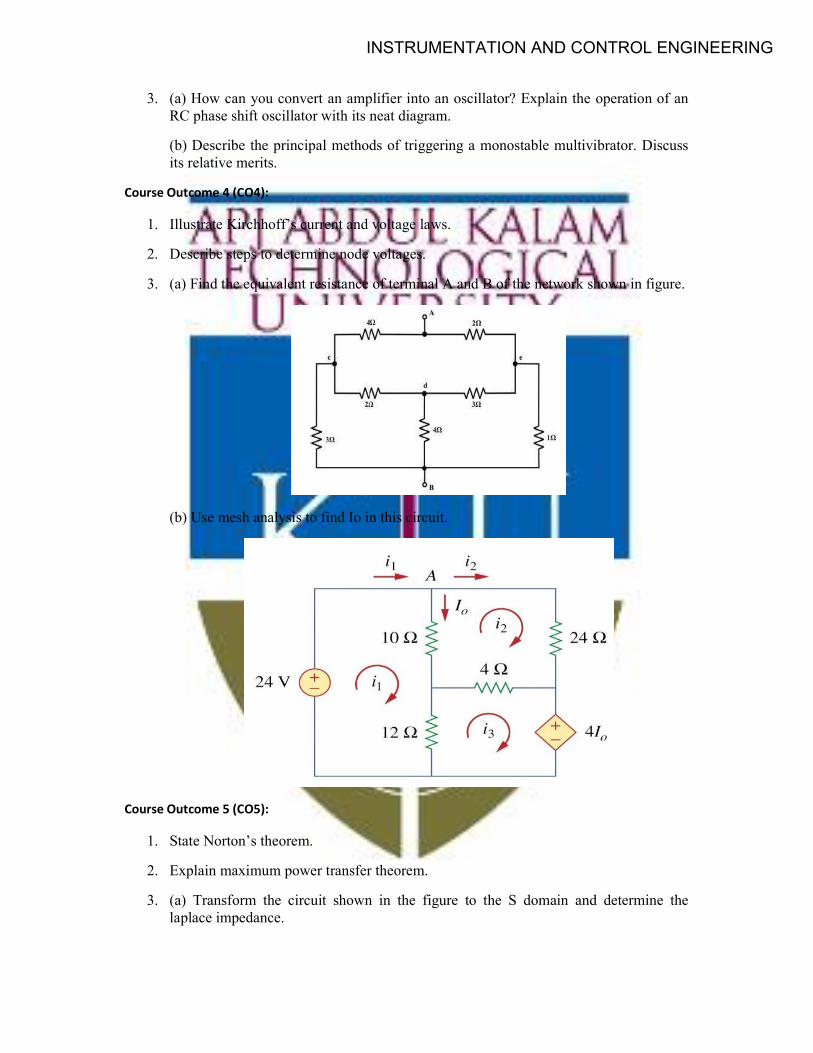
3. (a) Find the equivalent resistance of terminal A and B of the network shown in figure.
(b) Use mesh analysis to find Io in this circuit.
Course Outcome 5 (CO5):
1. State Norton’s theorem.
2. Explain maximum power transfer theorem.
3. (a) Transform the circuit shown in the figure to the S domain and determine the laplace impedance.
INSTRUMENTATION AND CONTROL ENGINEERING
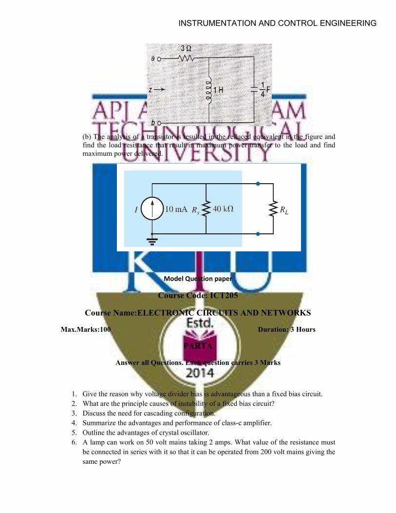
(b) The analysis of a transistor is resulted in the reduced equivalent in the figure and find the load resistance that result in maximum power transfer to the load and find maximum power delivered.
Model Question paper
Course Code: ICT205
Course Name:ELECTRONIC CIRCUITS AND NETWORKS
Max.Marks:100 Duration: 3 Hours
PARTA
Answer all Questions. Each question carries 3 Marks
1. Give the reason why voltage divider bias is advantageous than a fixed bias circuit. 2. What are the principle causes of instability of a fixed bias circuit? 3. Discuss the need for cascading configuration. 4. Summarize the advantages and performance of class-c amplifier. 5. Outline the advantages of crystal oscillator. 6. A lamp can work on 50 volt mains taking 2 amps. What value of the resistance must
be connected in series with it so that it can be operated from 200 volt mains giving the same power?
INSTRUMENTATION AND CONTROL ENGINEERING
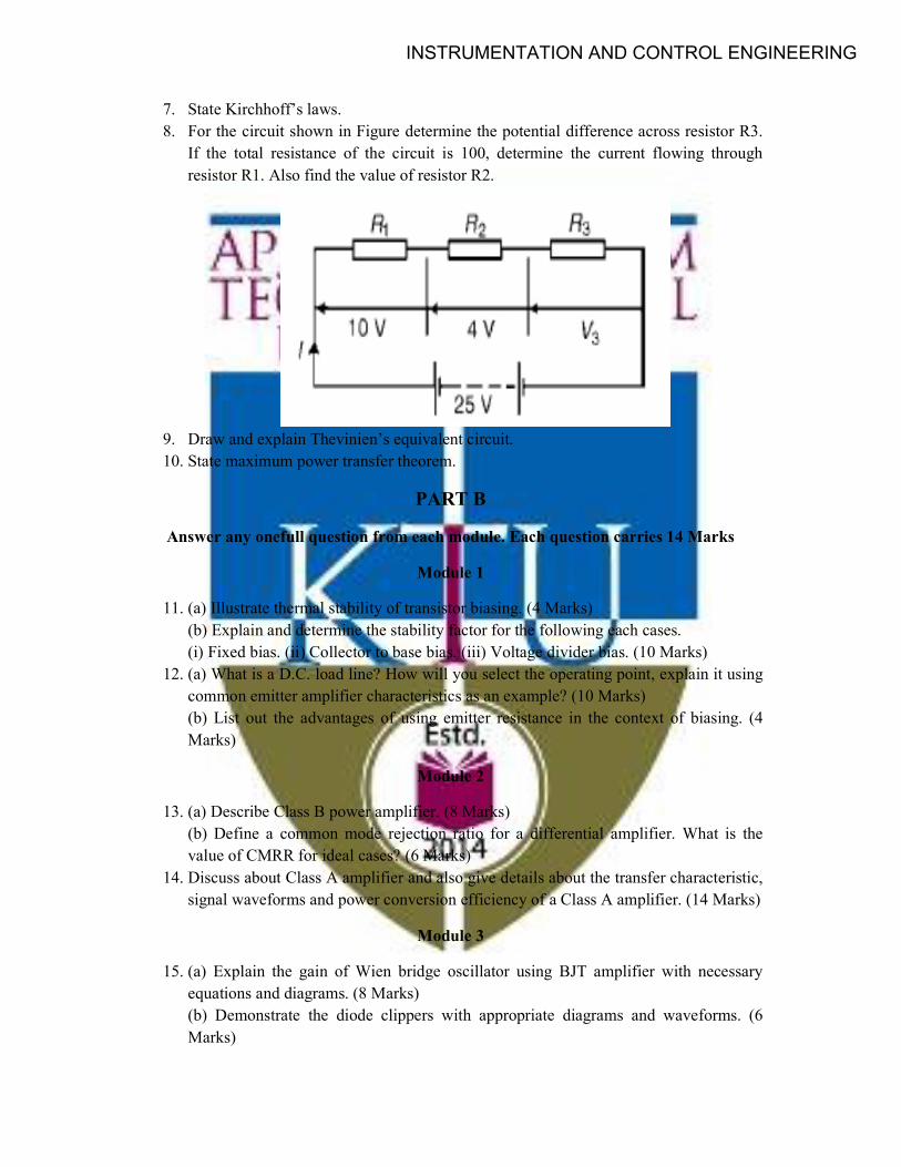
7. State Kirchhoff’s laws. 8. For the circuit shown in Figure determine the potential difference across resistor R3.
If the total resistance of the circuit is 100, determine the current flowing through resistor R1. Also find the value of resistor R2.
9. Draw and explain Thevinien’s equivalent circuit. 10. State maximum power transfer theorem.
PART B
Answer any onefull question from each module. Each question carries 14 Marks
Module 1
11. (a) Illustrate thermal stability of transistor biasing. (4 Marks) (b) Explain and determine the stability factor for the following each cases. (i) Fixed bias. (ii) Collector to base bias. (iii) Voltage divider bias. (10 Marks)
12. (a) What is a D.C. load line? How will you select the operating point, explain it using common emitter amplifier characteristics as an example? (10 Marks) (b) List out the advantages of using emitter resistance in the context of biasing. (4 Marks)
Module 2
13. (a) Describe Class B power amplifier. (8 Marks) (b) Define a common mode rejection ratio for a differential amplifier. What is the value of CMRR for ideal cases? (6 Marks)
14. Discuss about Class A amplifier and also give details about the transfer characteristic, signal waveforms and power conversion efficiency of a Class A amplifier. (14 Marks)
Module 3
15. (a) Explain the gain of Wien bridge oscillator using BJT amplifier with necessary equations and diagrams. (8 Marks) (b) Demonstrate the diode clippers with appropriate diagrams and waveforms. (6 Marks)
INSTRUMENTATION AND CONTROL ENGINEERING
16. (a) Evaluating the working principle of Bistable multivibrator with neat diagrams. (8 Marks) (b) Write a note on RC integrator and differentiator circuit. (6 Marks)
Module 4
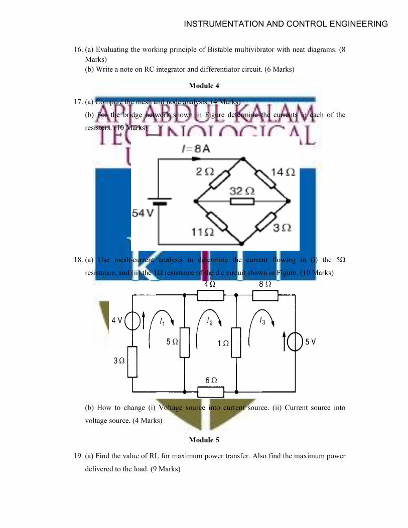
17. (a) Compare the mesh and node analysis. (4 Marks)
(b) For the bridge network shown in Figure determine the currents in each of the
resistors. (10 Marks)
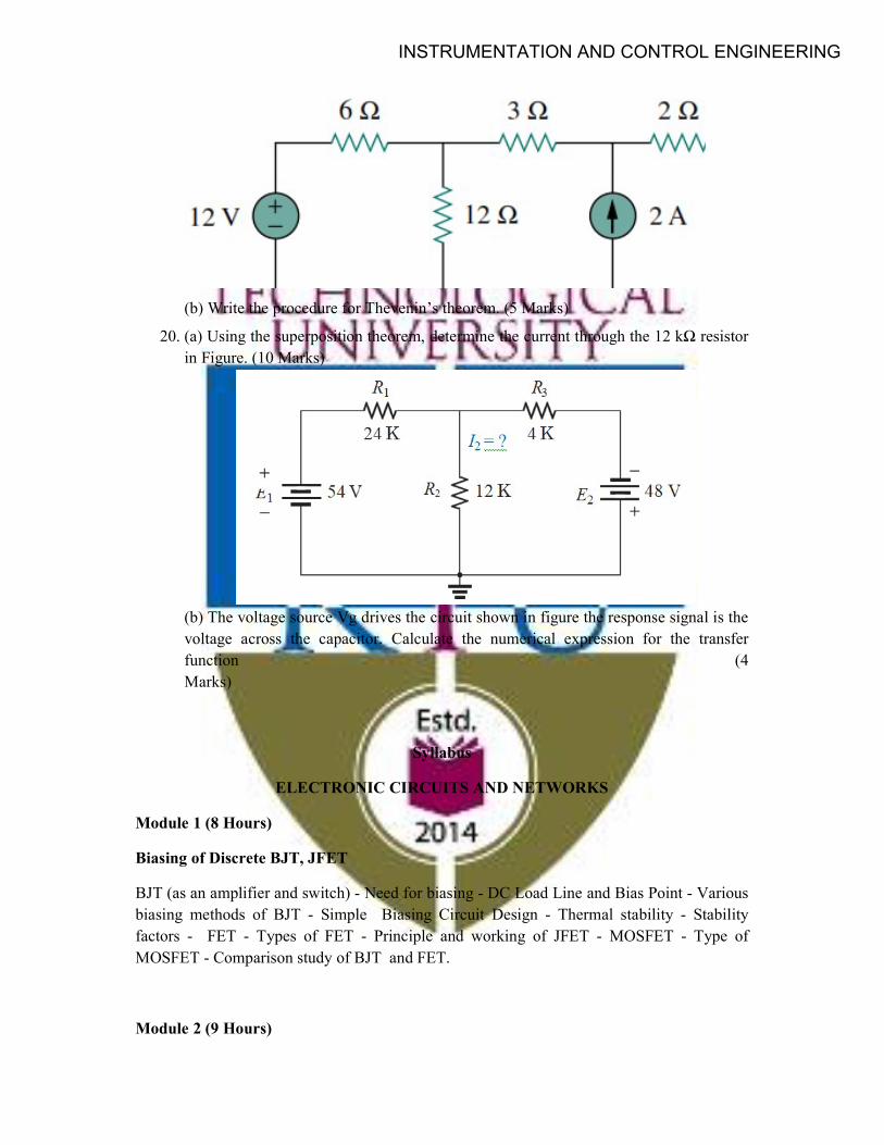
18. (a) Use mesh-current analysis to determine the current flowing in (i) the 5Ω
resistance, and (ii) the 1Ω resistance of the d.c circuit shown in Figure. (10 Marks)
(b) How to change (i) Voltage source into current source. (ii) Current source into
voltage source. (4 Marks)
Module 5
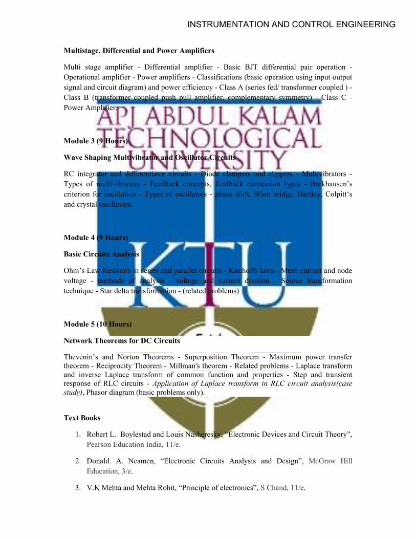
19. (a) Find the value of RL for maximum power transfer. Also find the maximum power
delivered to the load. (9 Marks)
INSTRUMENTATION AND CONTROL ENGINEERING
(b) Write the procedure for Thevenin’s theorem. (5 Marks)
20. (a) Using the superposition theorem, determine the current through the 12 kΩ resistor in Figure. (10 Marks)
(b) The voltage source Vg drives the circuit shown in figure the response signal is the voltage across the capacitor. Calculate the numerical expression for the transfer function (4 Marks)
Syllabus
ELECTRONIC CIRCUITS AND NETWORKS
Module 1 (8 Hours)
Biasing of Discrete BJT, JFET
BJT (as an amplifier and switch) - Need for biasing - DC Load Line and Bias Point - Various biasing methods of BJT - Simple Biasing Circuit Design - Thermal stability - Stability factors - FET - Types of FET - Principle and working of JFET - MOSFET - Type of MOSFET - Comparison study of BJT and FET.
Module 2 (9 Hours)
INSTRUMENTATION AND CONTROL ENGINEERING
Multistage, Differential and Power Amplifiers
Multi stage amplifier - Differential amplifier - Basic BJT differential pair operation - Operational amplifier - Power amplifiers - Classifications (basic operation using input output signal and circuit diagram) and power efficiency - Class A (series fed/ transformer coupled ) -Class B (transformer coupled push pull amplifier, complementary symmetry) - Class C -Power Amplifier.
Module 3 (9 Hours)
Wave Shaping Multivibrator and Oscillator Circuits
RC integrator and differentiator circuits - Diode clampers and clippers - Multivibrators - Types of multivibrators - Feedback concepts, feedback connection types - Barkhausen’s criterion for oscillation - Types of oscillators - phase shift, Wien bridge, Hartley, Colpitt‘s and crystal oscillators.
Module 4 (9 Hours)
Basic Circuits Analysis
Ohm’s Law Resistors in series and parallel circuits - Kirchoffs laws - Mesh current and node voltage - methods of analysis - voltage and current division - Source transformation technique - Star delta transformation - (related problems)
Module 5 (10 Hours)
Network Theorems for DC Circuits
Thevenin’s and Norton Theorems - Superposition Theorem - Maximum power transfer theorem - Reciprocity Theorem - Millman's theorem - Related problems - Laplace transform and inverse Laplace transform of common function and properties - Step and transient response of RLC circuits - Application of Laplace transform in RLC circuit analysis(case study), Phasor diagram (basic problems only).
Text Books
1. Robert L. Boylestad and Louis Nasheresky, “Electronic Devices and Circuit Theory”, Pearson Education India, 11/e.
2. Donald. A. Neamen, “Electronic Circuits Analysis and Design”, McGraw Hill Education, 3/e.
3. V.K Mehta and Mehta Rohit, “Principle of electronics”, S Chand, 11/e.
INSTRUMENTATION AND CONTROL ENGINEERING
4. A Sudhakar and Syammohan s pillai, “Circuits and Networks analysis and synthesis”, McGraw Hill Education, 5/e.
5. Ashfaq Hussain, “Networks and systems”, Khanna Book Publishing Co. (P) Ltd., 2/e.
Reference Books
1. Millman J, Halkias.C and Sathyabrada Jit, “Electronic Devices and Circuits”, McGraw Hill Education, 4/e.
2. Mahadevan, K., Chitra, C., “Electric Circuits Analysis”, PHI Learning Pvt. Ltd, 2/e.
3. M E Van Valkenburg, “Network Analysis”, Pearson Education, 3/e.
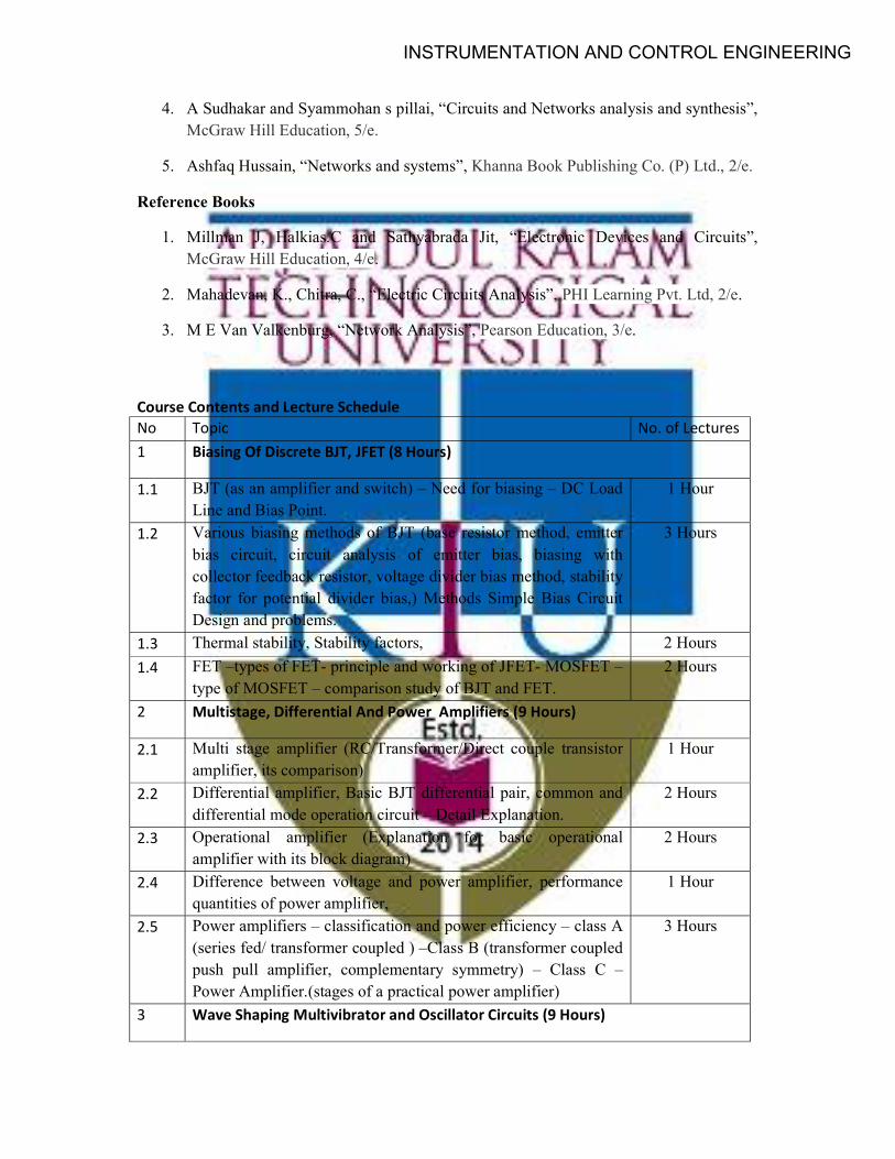
Course Contents and Lecture Schedule No Topic No. of Lectures 1 Biasing Of Discrete BJT, JFET (8 Hours)
1.1 BJT (as an amplifier and switch) – Need for biasing – DC Load Line and Bias Point.
1 Hour
1.2 Various biasing methods of BJT (base resistor method, emitter bias circuit, circuit analysis of emitter bias, biasing with collector feedback resistor, voltage divider bias method, stability factor for potential divider bias,) Methods Simple Bias Circuit Design and problems.
3 Hours
1.3 Thermal stability, Stability factors, 2 Hours
1.4 FET –types of FET- principle and working of JFET- MOSFET – type of MOSFET – comparison study of BJT and FET.
2 Hours
2 Multistage, Differential And Power Amplifiers (9 Hours)
2.1 Multi stage amplifier (RC/Transformer/Direct couple transistor amplifier, its comparison)
1 Hour
2.2 Differential amplifier, Basic BJT differential pair, common and differential mode operation circuit – Detail Explanation.
2 Hours
2.3 Operational amplifier (Explanation for basic operational amplifier with its block diagram)
2 Hours
2.4 Difference between voltage and power amplifier, performance quantities of power amplifier,
1 Hour
2.5 Power amplifiers – classification and power efficiency – class A (series fed/ transformer coupled ) –Class B (transformer coupled push pull amplifier, complementary symmetry) – Class C –Power Amplifier.(stages of a practical power amplifier)
3 Hours
3 Wave Shaping Multivibrator and Oscillator Circuits (9 Hours)
INSTRUMENTATION AND CONTROL ENGINEERING
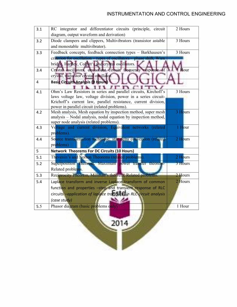
3.1 RC integrator and differentiator circuits (principle, circuit diagram, output waveform and derivation)
2 Hours
3.2 Diode clampers and clippers, Multivibrators (transistor astable and monostable multivibrator).
3 Hours
3.3 Feedback concepts, feedback connection types – Barkhausen’s criterion for oscillation – types of oscillators – phase shift, Wien bridge, Hartley, Colpitt‘s and crystal oscillators.
3 Hours
3.4 Crystal oscillators, equivalent circuit, frequency response of crystal, transistor crystal oscillator.
1 Hour
4 Basic Circuits Analysis (9 Hours)
4.1 Ohm’s Law Resistors in series and parallel circuits, Kirchoff’s laws voltage law, voltage division, power in a series circuit- Krichoff’s current law, parallel resistance, current division, power in parallel circuit (related problems).
3 Hours
4.2 Mesh analysis, Mesh equation by inspection method, super mesh analysis – Nodal analysis, nodal equation by inspection method, super node analysis (related problems).
3 Hours
4.3 Voltage and current division, Equivalent networks (related problems).
1 Hour
4.4 Source transformation technique, star delta conversion (related problems)
2 Hours
5 Network Theorems For DC Circuits (10 Hours) 5.1 Thevenin’s and Norton Theorems (related problems). 2 Hours
5.2 Superposition Theorem, Maximum power transfer theorem- Related problems.
3 Hours
5.3 Reciprocity Theorem, Millman’s theorem, Related problems. 2 Hours
5.4 Laplace transform and inverse Laplace transform of common function and properties –step and transient response of RLC circuits –application of laplace transform in RLC circuit analysis (case study)
2 Hours
5.5 Phasor diagram (basic problems only) 1 Hour
INSTRUMENTATION AND CONTROL ENGINEERING
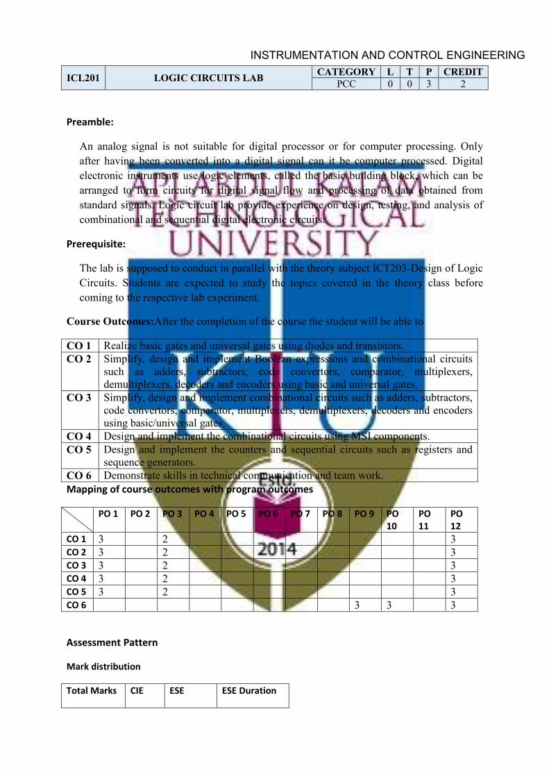
ICL201 LOGIC CIRCUITS LAB CATEGORY L T P CREDIT PCC 0 0 3 2
Preamble:
An analog signal is not suitable for digital processor or for computer processing. Only after having been converted into a digital signal can it be computer processed. Digital electronic instruments use logic elements, called the basic building block, which can be arranged to form circuits for digital signal flow and processing of data obtained from standard signals. Logic circuit lab provide experience on design, testing, and analysis of combinational and sequential digital electronic circuits.
Prerequisite:
The lab is supposed to conduct in parallel with the theory subject ICT203-Design of Logic Circuits. Students are expected to study the topics covered in the theory class before coming to the respective lab experiment.
Course Outcomes:After the completion of the course the student will be able to
CO 1 Realize basic gates and universal gates using diodes and transistors. CO 2 Simplify, design and implement Boolean expressions and combinational circuits
such as adders, subtractors, code convertors, comparator, multiplexers, demultiplexers, decoders and encoders using basic and universal gates.
CO 3 Simplify, design and implement combinational circuits such as adders, subtractors, code convertors, comparator, multiplexers, demultiplexers, decoders and encoders using basic/universal gates.
CO 4 Design and implement the combinational circuits using MSI components. CO 5 Design and implement the counters and sequential circuits such as registers and
sequence generators. CO 6 Demonstrate skills in technical communication and team work. Mapping of course outcomes with program outcomes
PO 1 PO 2 PO 3 PO 4 PO 5 PO 6 PO 7 PO 8 PO 9 PO 10
PO 11
PO 12
CO 1 3 2 3 CO 2 3 2 3 CO 3 3 2 3 CO 4 3 2 3 CO 5 3 2 3 CO 6 3 3 3
Assessment Pattern
Mark distribution
Total Marks CIE ESE ESE Duration
INSTRUMENTATION AND CONTROL ENGINEERING
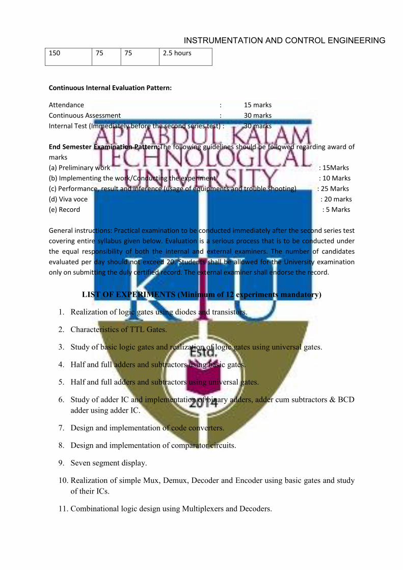
150 75 75 2.5 hours
Continuous Internal Evaluation Pattern:
Attendance : 15 marks Continuous Assessment : 30 marks Internal Test (Immediately before the second series test) : 30 marks End Semester Examination Pattern:The following guidelines should be followed regarding award of marks (a) Preliminary work : 15Marks (b) Implementing the work/Conducting the experiment : 10 Marks (c) Performance, result and inference (usage of equipments and trouble shooting) : 25 Marks (d) Viva voce : 20 marks (e) Record : 5 Marks General instructions: Practical examination to be conducted immediately after the second series test covering entire syllabus given below. Evaluation is a serious process that is to be conducted under the equal responsibility of both the internal and external examiners. The number of candidates evaluated per day should not exceed 20. Students shall be allowed for the University examination only on submitting the duly certified record. The external examiner shall endorse the record.
LIST OF EXPERIMENTS (Minimum of 12 experiments mandatory)
1. Realization of logic gates using diodes and transistors.
2. Characteristics of TTL Gates.
3. Study of basic logic gates and realization of logic gates using universal gates.
4. Half and full adders and subtractors using basic gates.
5. Half and full adders and subtractors using universal gates.
6. Study of adder IC and implementation of binary adders, adder cum subtractors & BCD adder using adder IC.
7. Design and implementation of code converters.
8. Design and implementation of comparator circuits.
9. Seven segment display.
10. Realization of simple Mux, Demux, Decoder and Encoder using basic gates and study of their ICs.
11. Combinational logic design using Multiplexers and Decoders.
INSTRUMENTATION AND CONTROL ENGINEERING
12. Flip-Flop Circuits (SR, JK, T, D and Master Slave JK) using basic gates.
13. Study of flip flop ICs.
14. Asynchronous Counters.
15. Johnson and Ring Counters.
16. Synchronous counters.
17. Study of counter ICs.
18. A sequence generator circuit.
19. A sequence detector Circuit.
20. Shift registers using flip flops.
Text Books
1. Charles H. Roth, Jr. “Fundamentals of Logic Design”, Cengage Learning India Private Limited, 7/e.
2. Anand Kumar, “Fundamentals of Digital Circuits”, PHI learning, 3/e, 2010, ISBN: 978-81-203-3679-7.
3. Stephen Brown and Zvonko Vranesic, “Fundamentals of Digital Logic with VHDL Design”, McGraw Hill Education, 2/e.
Reference Books
1. Thomas L Floyd, “Digital Fundamentals”, Pearson, 11/e, 2011.
2. John F Wakerly, “Digital Design- Principles and Practices”, Pearson Education, 4/e.
3. Taub and Schilling, “Digital principles and applications”, TMH.
4. Mano M, “Digital Design”, Pearson Education India, 5/e.
5. R P Jain, “Modern Digital Electronics”, McGraw Hill Education, 4/e.
INSTRUMENTATION AND CONTROL ENGINEERING
ICL203 ELECTRONIC DEVICES AND CIRCUITS LAB
CATEGORY L T P CREDIT PCC 0 0 3 2
Preamble:
To make students familiar with the design of electronic circuits using passive and active components and make them understand the capabilities and applications of such circuits.
Prerequisite:
EST130 Basic Electrical and Electronics Engineering, ESL130 Electrical and Electronics Workshop and ICT205 Electronic Circuits and Networks. Since the lab runs in parallel with the theory subject ICT205 Electronic Circuits and Networks, students are expected to study the topics covered in the theory class before coming to lab.
Course Outcomes: After the completion of the course the student will be able to
CO 1 Analyse the characteristics of discrete components. CO 2 Design wave shaping circuits, sweep circuits, and switch circuits using discrete
components. CO 3 Design low pass and high pass filter circuits. CO 4 Design voltage regulator, power supply circuits using discrete components. CO 5 Design differentiator, integrator, oscillator and amplifier. CO 6 Demonstrate skills in team work, technical communication and documenting an
experimental work. Mapping of course outcomes with program outcomes
PO 1 PO 2 PO 3 PO 4 PO 5 PO 6 PO 7 PO 8 PO 9 PO 10
PO 11
PO 12
CO 1 3 2 3 CO 2 3 3 3 CO 3 3 3 3 CO 4 3 3 3 CO 5 3 3 3 CO 6 3 3
Assessment Pattern
Mark distribution
Total Marks CIE ESE ESE Duration
150 75 75 2.5 hours
Continuous Internal Evaluation Pattern:
Attendance : 15 marks
INSTRUMENTATION AND CONTROL ENGINEERING
Continuous Assessment : 30 marks Internal Test (Immediately before the second series test) : 30 marks End Semester Examination Pattern:The following guidelines should be followed regarding award of marks (a) Preliminary work : 15Marks (b) Implementing the work/Conducting the experiment : 10 Marks (c) Performance, result and inference (usage of equipment and trouble shooting) : 25 Marks (d) Viva voce : 20 marks (e) Record : 5 Marks General instructions: Practical examination to be conducted immediately after the second series test covering entire syllabus given below. Evaluation is a serious process that is to be conducted under the equal responsibility of both the internal and external examiners. The number of candidates evaluated per day should not exceed 20. Students shall be allowed for the University examination only on submitting the duly certified record. The external examiner shall endorse the record.
LIST OF EXPERIMENTS
1. Characteristics of diodes (Si and Ge diodes, &Zener diode). 2. Rectifying circuits.
(i) Half Wave rectifier, ii) Centre tapped Full Wave rectifier, and iii) Full Wave Bridge rectifier.
3. Filter circuits - Capacitor filter, inductor filter and Pi section filter. 4. Clipping circuits. 5. Clamping circuits. 6. Characteristics of transistors. 7. Biasing of BJT – Fixed and voltage divider biasing. 8. Series voltage regulator using transistors. 9. Zener voltage regulator. 10. Frequency responses of RC low pass & high pass filters. 11. RC differentiating and integrating circuits. 12. Characteristics of FET. 13. Design of single and dual power supplies. 14. Biasing of FET – Fixed and voltage divider biasing. 15. RC phase shift oscillator. 16. Wein Bridge Oscillator. 17. Hartley and Colpitts oscillator. 18. Switch circuits using BJTs. 19. Sweep circuits - Simple transistor and bootstrap sweep circuits. 20. RC coupled amplifiers using BJT with and without feedback.
INSTRUMENTATION AND CONTROL ENGINEERING
Text Books
1. R E Boylstead and L Nashelsky, “Electronic Devices and Circuit Theory”, Pearson Education, 11/e.
2. Bernard Grob, “Basic Electronics”, McGraw Hill Education.
Reference Books
1. Adel S. Sedra& Kenneth C. Smith, “Microelectronic Circuits: Theory and Applications”, Oxford University Press. 7/e.
2. Gray& Meyer, “Analysis and Design of Analog Integrated Circuits”, Wiley, 5/e.
INSTRUMENTATION AND CONTROL ENGINEERING

SEMESTER -3
MINOR
INSTRUMENTATION AND CONTROL ENGINEERING
ICT281 INTRODUCTION TO SENSORS AND TRANSDUCERS
CATEGORY L T P CREDIT VAC 3 1 0 4
Preamble:
The aim of the Sensors and Transducers course is:
1) To make students familiar with the constructions and working principles of different types of sensors and transducers.
2) To learn the static and dynamic characteristics of the measuring instruments. 3) To familiarize with a variety of transducers, which are very vital in instrumentation
systems.
Course Outcomes:
After the completion of the course the student will be able to
CO 1 Explain the concept, application and functional elements of sensors and transducers.
CO 2 Describe the static and dynamic characteristics of the measuring instruments.
CO 3 Explainthe resistive, inductive and capacitive transducers which is used to convert a physical parameter into an electrical quantity.
CO 4 Explain the principle and operation of transducers used for the measurement of temperature, strain, motion, position and light.
CO 5 Explain the concept of process of calibration.
CO 6 Explain different types of errors that can occur during the measurement, and the methods used to correct the measurement errors.
Mapping of course outcomes with program outcomes
PO 1 PO 2 PO 3 PO 4 PO 5 PO 6 PO 7 PO 8 PO 9 PO 10 PO 11 PO 12 CO 1 2 3 CO 2 2 3 CO 3 2 3 CO 4 2 3 CO 5 3 2 3 CO 6 3 3 Assessment Pattern
Bloom’s Category Continuous Assessment Tests End Semester Examination 1 2
Remember 10 10 30 Understand 40 40 70 Apply
INSTRUMENTATION AND CONTROL ENGINEERING
Analyse Evaluate Create
Mark distribution
Total Marks CIE ESE ESE Duration
150 50 100 3 hours
Continuous Internal Evaluation Pattern:
Attendance : 10 marks Continuous Assessment Test (2 numbers) : 25 marks Assignment/Quiz/Course project : 15 marks
End Semester Examination Pattern:
There will be two parts; Part A and Part B. Part A contains 10 questions with 2 questions from each module, having 3 marks for each question. Students should answer all questions. Part B contains 2 questions from each module of which student should answer any one. Each question can have maximum 2 sub-divisions and carry 14 marks.
Course Level Assessment Questions
Course Outcome 1 (CO1):
1. Define sensor.
2. Compare sensor and transducer.
3. Classification of transducers.
4. Give the functional elements of an instrumentation system.
Course Outcome 2 (CO2):
1. Define static and dynamic characteristics with suitable example.
2. Compare drift and accuracy.
Course Outcome 3 (CO3):
1. Give the principle and working of any two resistive transducer
2. How LVDT can be used for the measurement of displacement.
3. Describe the concept of smart sensors.
Course Outcome 4 (CO4):
INSTRUMENTATION AND CONTROL ENGINEERING
1. Compare thermistor, RTD and thermocouple.
2. Explain the working of photo-voltaic cell.
3. Describe sensor based on Villari effect for assessment of motion, force and torque.
Course Outcome 5 (CO5):
1. Give the concept of absolute and secondary instruments.
2. Describe the concept of calibration with suitable example.
Course Outcome 6 (CO6):
1. Classify different types of errors.
2. Concept of loading effect and its effect on shunt and series connected instruments.
3. Eliminating methods of different errors.
Model Question paper
Course Code: ICT281
Course Name:INTRODUCTION TO SENSORS AND TRANSDUCERS
Max.Marks:100 Duration: 3 Hours
PARTA
Answer all Questions. Each question carries 3 Marks
1. Compare sensor and transducer with suitable examples. 2. Define dump and intelligent instruments, with suitable example in day to day life. 3. Why we need standards? Justify your answer with suitable examples. 4. Give the concept of interfering inputs with examples. 5. How a strain gauge is working as a resistive transducer. 6. Give the working of variable area capacitors, with suitable applications. 7. What is the need of a range of thermal sensors instead of one? 8. Explain the working of solar cell. 9. Compare static and dynamic characteristic. 10. Define loading effects, is it is desirable or not? Why?
PART B
Answer any onefull question from each module. Each question carries 14 Marks
Module 1
INSTRUMENTATION AND CONTROL ENGINEERING
11. Give the functional elements of a measurement system with a suitable example. 12. Classify measuring instruments. Minimum five classifications with examples.
Module 2
13. Why we are configuring a system? Explain input output configuration of measuring an instrument with example.
14. How modifying inputs are get into a measuring instrument? Give thecorrection for interfering and modifying inputs.
Module 3
15. Derive the gauge factor of a strain gauge and give its significant in the measurement of strain.
16. Give the constructional details of LVDT.
Module 4
17. Compare RTD, Thermocouple and Thermistor.
18. What you meant by villari effect? How it is useful in analysing different parameters
such as force, torque and proximity.
Module 5
19. Explain desirable and non-desirable characteristics of a measurement system, with
suitable examples.
20. How input impedance and output impedance are related to the loading effect.
Syllabus
INTRODUCTION TO SENSORS AND TRANSDUCERS
Module 1 (10 Hours)
Introduction to Sensor and Their Applications
Introduction to sensors and transducer; compare sensor and transducer; Functional elements of a measurement system and examples; Basic description of the functional elements of the instruments.
Classification of sensors/transducers
Absolute and secondary instruments; Deflection and null type; manually operated and automatic type; analogue and digital types; self-generating and power operated types; contacting and non-contacting types; dumb and intelligent types.
INSTRUMENTATION AND CONTROL ENGINEERING
Module 2 (10 Hours)
Standards and Calibration
Concept of standards; Concept and definition of calibration; Input output configuration of measuring instruments and measurement systems.
Inputs
Desired inputs; interfering inputs; modifying inputs; methods of correction for interfering and modifying inputs.
Module 3 (8 Hours)
Resistive, Capacitive and Inductive transducers
Resistive (potentiometric type): Forms, material, resolution, accuracy, sensitivity; Strain gauge: Theory, type, materials, design consideration, sensitivity, gauge factor, variation with temperature and compensation, adhesive, rosettes; Capacitive: Variable distance-parallel plate type, variable area- parallel plate, serrated plate/teeth type and cylindrical type, variable dielectric constant type, calculation of sensitivity; Inductive: Mutual inductance change type, transformer action type; LVDT: Construction, material, output input relationship, I/O curve.
Module 4 (9 Hours)
Thermal Sensors
Thermocouple; Material expansion type: solid, liquid, gas & vapour; Resistance change type: RTD, Thermistor, material, shape, ranges and accuracy specification; Thermo-emf sensor: types, thermoelectric power, general consideration, Junction semiconductor type IC and PTAT type.
Magnetic Sensors
Sensor based on Villari effect for assessment of force, torque, proximity, Thomson effect, Hall Effect, performance characteristics; Radiation sensors: LDR, Photovoltaic cells, photodiodes, photo emissive cell types, materials, construction, response. Geiger counters, Scintillation detectors, Introduction to smart sensors.
Module 5 (8 Hours)
Measurement System Performance
INSTRUMENTATION AND CONTROL ENGINEERING
Measurement System performance. Static and dynamic characteristics. Errors in measurements, true value, static error, static correction. Scale range and span. Error calibration curve, reproducibility and drift, repeatability, noise, signal to noise ratio, sources of noise, Johnson noise, power spectrum density, noise. Accuracy and precision, static sensitivity, linearity, hysteresis, threshold, dead time. Dead zone, resolution or discrimination. Loading effects. Input impedances, input admittance, output impedances, output admittance. Loading effects due to shunt connected instruments. Loading effects due to series connected instruments.
Text Books
1. Ernest.ODoeblin, “Measurement Systems”, McGraw Hill Education, 6/e.
Reference Books
1. A.K Sawhney, “A Course In Mechanical Measurements And Instrumentation & Control”, Dhanpat Rai & Co.
2. C.S. Rangan, G.R. Sarma, and V.S.V. Mani, “Instrumentation: Devices and Systems”, McGraw Hill Education, 2/e.
3. DVS Murthy, “Transducers and Instrumentation”, Prentice Hall India Learning Private Limited, 2/e.
4. D. Patranabis, “Sensors and Transducers”, Prentice Hall India Learning Private Limited, 2/e.
Course Contents and Lecture Schedule No Topic No. of Lectures 1 Introduction to Sensor and Their Applications (4 Hours)
1.1 Introduction to sensors and transducer; compare sensor and transducer.
2 Hours
1.2 Functional elements of a measurement system and examples; Basic description of the functional elements of the instruments.
2 Hours
Classification of sensors/transducers (6 Hours) 1.3 Absolute and secondary instruments; Deflection and null type;
manually operated and automatic type; analogue and digital types; self-generating and power operated types; contacting and non-contacting types; dumb and intelligent types.
6 Hours
2 Standards and Calibration (5 Hours)
INSTRUMENTATION AND CONTROL ENGINEERING
2.1 Concept of standards. Examples. 1 Hour 2.2 Concept and definition of Calibration with an example 2 Hours 2.3 Input output configuration of measuring instruments and
measurement systems. 2 Hours
Inputs (5 Hours) 2.4 Desired inputs, interfering inputs, modifying inputs. 2 Hours 2.5 Methods of correction for interfering and modifying inputs. 3 Hours 3 Resistive, Capacitive and Inductive transducers (8 Hours)
3.1 Resistive (potentiometric type): Forms, material, resolution, accuracy, sensitivity
2 Hours
3.2 Strain gauge: Theory, type, materials, design consideration, sensitivity, gauge factor, variation with temperature and compensation, adhesive, rosettes.
2 Hours
3.3 Capacitive: Variable distance-parallel plate type, variable area- parallel plate, serrated plate/teeth type and cylindrical type, variable dielectric constant type, calculation of sensitivity.
2 Hours
3.4 Inductive: Mutual inductance change type, transformer action type; LVDT: Construction, material, output input relationship, I/O curve
2 Hours
4 Thermal Sensors (4 Hours)
4.1 Thermocouple; Material expansion type: solid, liquid, gas & vapour
1 Hour
4.2 Resistance change type: RTD, Thermistor, material, shape, ranges and accuracy specification; Thermo-emf sensor: types, thermoelectric power, general consideration, Junction semiconductor type IC and PTAT type.
3 Hours
Magnetic Sensors (5 Hours) 4.3 Sensor based on Villari effect for assessment of force, torque,
proximity, Thomson effect, Hall Effect, performance characteristics.
3 Hours
4.4 Radiation sensors: LDR, Photovoltaic cells, photodiodes, photo emissive cell types, materials, construction, response. Geiger counters, Scintillation detectors, Introduction to smart sensors.
2 Hour
5 Measurement System Performance (8 Hours) 5.1 Measurement System performance. Static and dynamic
characteristics. 2 Hours
5.2 Errors in measurements, true value, static error, static correction. Scale range and span. Error calibration curve, reproducibility and drift, repeatability, noise, signal to noise ratio, sources of noise, Johnson noise, power spectrum density, noise. Accuracy and precision, static sensitivity, linearity, hysteresis, threshold, dead time. Dead zone, resolution or discrimination.
3 Hours
INSTRUMENTATION AND CONTROL ENGINEERING
5.3 Loading effects. Input impedances, input admittance, output impedances, output admittance.
1 Hour
5.4 Loading effects due to shunt connected instruments. Loading effects due to series connected instruments.
2 Hours
INSTRUMENTATION AND CONTROL ENGINEERING

ICT283 CIRCUIT DESIGN ANALYSIS FOR INSTRUMENTATION
CATEGORY L T P CREDIT VAC 3 1 0 4
Preamble:
The aim of the Circuit Design and Analysis for Instrumentation course is to enable the students to understand the foundation of circuit design and analysis used for instrumentation applications.
Prerequisite:
Basic electrical network analysis, Electronic Circuits and Devices.
Course Outcomes:
After the completion of the course the student will be able to
CO 1 Discuss types of the SPICE software.
CO 2 Do DC analysis of a circuit.
CO 3 Do transient analysis of a circuit.
CO 4 Do AC analysis of a circuit.
CO 5 Model Diode, Bipolar Junction Transistor, JFET and MOSFET.
Mapping of course outcomes with program outcomes
PO 1 PO 2 PO 3 PO 4 PO 5 PO 6 PO 7 PO 8 PO 9 PO 10 PO 11 PO 12 CO 1 2 2 CO 2 3 3 3 CO 3 3 3 3 CO 4 3 3 3 CO 5 3 3 3
Assessment Pattern
Bloom’s Category Continuous Assessment Tests End Semester Examination 1 2
Remember 3 3 Understand 23 13 36 Apply 24 37 61 Analyse Evaluate Create
INSTRUMENTATION AND CONTROL ENGINEERING
Mark distribution
Total Marks CIE ESE ESE Duration
150 50 100 3 hours
Continuous Internal Evaluation Pattern:
Attendance : 10 marks Continuous Assessment Test (2 numbers) : 25 marks Assignment/Quiz/Course project : 15 marks
End Semester Examination Pattern:
There will be two parts; Part A and Part B. Part A contains 10 questions with 2 questions from each module, having 3 marks for each question. Students should answer all questions. Part B contains 2 questions from each module of which student should answer any one. Each question can have maximum 2 sub-divisions and carry 14 marks.
Course Level Assessment Questions
Course Outcome 1 (CO1):
1. Explain the various types of analysis allowed by PSpice.
2. Mention the PSpice platform used for Spice version.
3. Explain the format for a circuit file.
Course Outcome 2 (CO2):
1. Model temperature dependent resistors.
2. Model dependent and independent voltage and current sources.
3. Explain the various commands used for DC analysis.
Course Outcome 3 (CO3):
1. Model transient voltage and current sources and specify their parameters.
2. Assign initial conditions for transient analysis.
Course Outcome 4 (CO4):
1. Model AC voltage and current sources and specify their parameters.
2. Model linear and nonlinear magnetic elements and specify their parameters.
3. Perform the AC analysis of a circuit and set its parameters.
INSTRUMENTATION AND CONTROL ENGINEERING

Course Outcome 5 (CO5):
1. Model a diode in SPICE and specify its mode parameters.
2. Model SPICE BJTs and specify SPICE model parameters.
3. Model SPICE FETs and specify SPICE model parameters.
Model Question paper
Course Code: ICT283
Course Name:CIRUIT DESIGN ANALYSIS FOR INSTRUMENTATION
Max.Marks:100 Duration: 3 Hours
PARTA
Answer all Questions. Each question carries 3 Marks
1. Mention the limitations of P Spice. 2. Write the format for a circuit file. 3. Explain model statement for modelling the operating temperature in P Spice. 4. Explain the types of output commands for DC circuit analysis using PSpice. 5. Draw the schematics of an exponential voltage source and pulse voltage source in
PSpice. 6. Explain the initial Transient Conditions statement and Transient analysis Statement. 7. Write the general form of Coupled inductor using PSpice. 8. Explain the AC output variables in PSpice5. 9. Write the model statement for an NPN and PNP BJT. 10. Write the PSpice model statement for a JFET.
PART B
Answer any onefull question from each module. Each question carries 14 Marks
Module 1
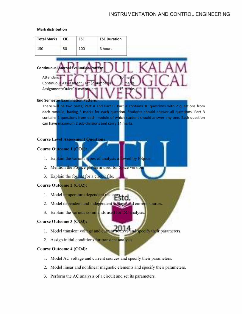
11. Explain the format of circuit file in PSpice with the help of a circuit. 12. Write the circuit file listings of the following circuit to print all node voltages.
INSTRUMENTATION AND CONTROL ENGINEERING
Module 2
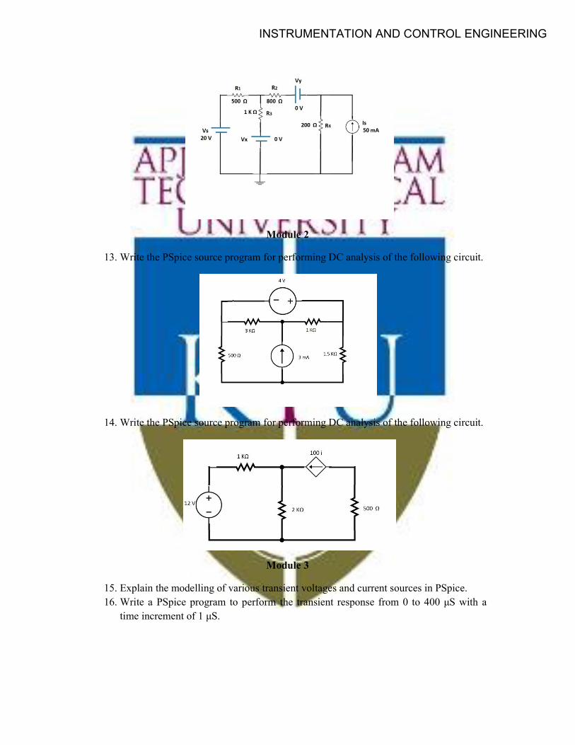
13. Write the PSpice source program for performing DC analysis of the following circuit.
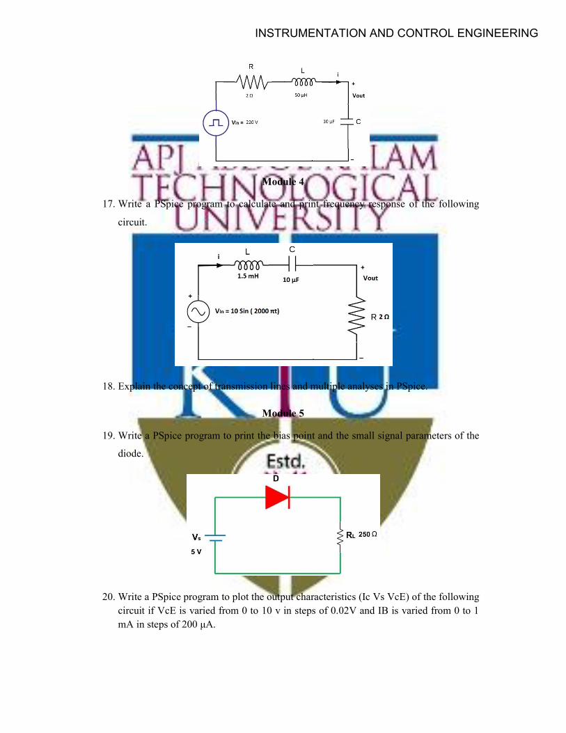
14. Write the PSpice source program for performing DC analysis of the following circuit.
Module 3
15. Explain the modelling of various transient voltages and current sources in PSpice. 16. Write a PSpice program to perform the transient response from 0 to 400 μS with a
time increment of 1 μS.
INSTRUMENTATION AND CONTROL ENGINEERING
Module 4
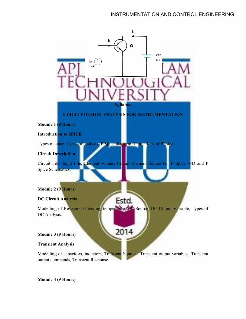
17. Write a PSpice program to calculate and print frequency response of the following
circuit.
18. Explain the concept of transmission lines and multiple analyses in PSpice.
Module 5
19. Write a PSpice program to print the bias point and the small signal parameters of the
diode.
20. Write a PSpice program to plot the output characteristics (Ic Vs VcE) of the following circuit if VcE is varied from 0 to 10 v in steps of 0.02V and IB is varied from 0 to 1 mA in steps of 200 μA.
INSTRUMENTATION AND CONTROL ENGINEERING
Syllabus
CIRCUIT DESIGN ANALYSIS FOR INSTRUMENTATION
Module 1 (8 Hours)
Introduction to SPICE
Types of spice, Types of analysis- P Spice platform, Limitations of PSpice.
Circuit Description
Circuit File, Input File, Element Values, Circuit Element Source-For P Spice A/D and P Spice Schematics.
Module 2 (9 Hours)
DC Circuit Analysis
Modelling of Resistors, Operating temperature, DC Source, DC Output Variable, Types of DC Analysis.
Module 3 (9 Hours)
Transient Analysis
Modelling of capacitors, inductors, Transient Sources, Transient output variables, Transient output commands, Transient Response.
Module 4 (9 Hours)
INSTRUMENTATION AND CONTROL ENGINEERING
AC Circuit Analysis
AC output variables, Independent AC sources, AC Analysis, Magnetic Elements-Mutual Inductors, Transmission lines, multiple analyses.
Module 5 (10 Hours)
Modelling of Dynamic Elements Diode Statement, Diode Parameters, Examples of DC and AC analysis, BJT Statement, BJT Parameters Examples of DC and AC analysis. JFET Statement, JFET Parameters, Examples of DC, Transient and AC analysis.
Text Books
1. Muhammad H Rashid, “Introduction to PSpice Using OrCAD for Circuits and Electronics”, Pearson Education, 3/e.
2. Boylestad and Nashelsky, “Electronic Devices and Circuits Theory”, Pearson, 11/e.
Reference Books
1. Robert Boylestad, “Introductory Circuit Analysis”, Pearson Education India, 12/e.
2. Irvine, “PSpice Manual”, California Microsim Corporation,1992.
3. Philip E Allen and D R Holberg, “CMOS Analog Circuit Design”, Oxford University Press, 3/e.
4. Jack F Morris, “Basic Circuit Analysis”, .New York: Houghton Mifflin, 1991.
Course Contents and Lecture Schedule No Topic No. of Lectures 1 Introduction to Spice (4 Hours)
1.1 Types of Spice, Types of Analysis-DC Analysis, AC Analysis, Transient Analysis.
2 Hour
1.2 P Spice Platform. 2 Hours Circuit Description (4 Hours)
1.3 Circuit File, Input File, Element Values Nodes, Circuit Element Source, Types of analysis, output variable, output files.
4 Hours
2 DC Circuit Analysis (9 Hours)
2.1 Modelling of Resistors, Operating temperature. 2 Hours
INSTRUMENTATION AND CONTROL ENGINEERING
2.2 DC Source –Independent DC Voltage Source, Independent DC Current Source, Dependent DC Voltage Source, Dependent DC Current Source.
3 Hours
2.3 DC Output Variable-Voltage Output, Current Output. 2 Hours 2.4 Types of DC Analysis-.OP,.TF,.DC,.PARAM. 2 Hours 3 Transient Analysis (9 Hours)
3.1 Modelling of capacitors, inductors. 2 Hours 3.2 Modelling of Transient Sources-Exponential Source, Piecewise
linear source, Single Frequency Modulation (SFFM), Independent Voltage and current Sources.
2 Hours
3.3 Transient output variables, Transient output commands. 3 Hours 3.4 Transient Response-.IC and .TRAN. 2 Hourss 4 AC Circuit Analysis (9 Hours)
4.1 AC output variables-Voltage output, Current output. 1 Hour 4.2 Independent AC sources. 1 Hour 4.3 AC Analysis. 2 Hours 4.4 Magnetic Elements-Mutual Inductors. 2 Hours 4.5 Transmission lines. 2 Hours 4.6 Multiple analyses. 1 Hour 5 Modelling of Dynamic Elements (10 Hours) 5.1 Diode Statement, Diode Parameters, Examples of DC and AC
analysis. 3 Hours
5.2 BJT Statement Parameters, Examples of DC and AC analysis. 4 Hours 5.3 JFET Statement, JFET Parameters, Examples of DC, Transient
and AC analysis. 3 Hours
INSTRUMENTATION AND CONTROL ENGINEERING
SEMESTER -4
INSTRUMENTATION AND CONTROL ENGINEERING
ICT202 MEASUREMENTS AND INSTRUMENTATION
CATEGORY L T P CREDIT PCC 3 1 0 4
Preamble:
The aim of the Measurements and Instrumentation course is to:
• Introduce the basics of indicating and storage instruments. • Enable the students to measure electrical quantities like power, resistance, inductance,
and capacitance. • Provide the basic principles of fluid characteristics. • Provide the basic principles of force, and torque measurement. • Enable the students to do linear and angular measurement.
Prerequisite:
Basic Electrical, and Transducer.
Course Outcomes:
After the completion of the course the student will be able to
CO 1 Explain the principle and operation of moving coil instruments.
CO 2 Determine power, resistance, inductance, and capacitance.
CO 3 Explain the principle and operation of storage & display devices.
CO 4 Examine the fluid static and dynamic characteristics.
CO 5 Explain the principles and operation of measuring systems used for force, and torque.
CO 6 Perform linear and angular measurement.
Mapping of course outcomes with program outcomes
PO 1 PO 2 PO 3 PO 4 PO 5 PO 6 PO 7 PO 8 PO 9 PO 10 PO 11 PO 12 CO 1 2 2 CO 2 3 3 CO 3 2 2 CO 4 3 3 CO 5 2 2 CO 6 3 3
INSTRUMENTATION AND CONTROL ENGINEERING
Assessment Pattern
Bloom’s Category Continuous Assessment Tests End Semester Examination 1 2
Remember Understand 26 36 62 Apply 24 14 38 Analyse Evaluate Create
Mark distribution
Total Marks CIE ESE ESE Duration
150 50 100 3 hours
Continuous Internal Evaluation Pattern:
Attendance : 10 marks Continuous Assessment Test (2 numbers) : 25 marks Assignment/Quiz/Course project : 15 marks
End Semester Examination Pattern:
There will be two parts; Part A and Part B. Part A contains 10 questions with 2 questions from each module, having 3 marks for each question. Students should answer all questions. Part B contains 2 questions from each module of which student should answer any one. Each question can have maximum 2 sub-divisions and carry 14 marks.
Course Level Assessment Questions
Course Outcome 1 (CO1):
1. Distinguish between gravity control and spring control used in indicating instruments.
Course Outcome 2 (CO2):
1. In an Anderson Bridge for the measurement of inductance the arm AB consists of an unknown impedance with inductance L and R, a known variable resistance in arm BC, fixed resistance of 600ohm each in arms CD and DA, a known variable resistance in arm DE, and a capacitor with fixed capacitance of 1microfarad in the arm CE. The AC supply of 100Hz is connected across A and C, and the detector is connected between B and E. If the balance is obtained with a resistance of 400ohm in the arm DE and a resistance of 800ohm in the arm BC, calculate the value of unknown R and L. Derive the conditions for balance.
2.
INSTRUMENTATION AND CONTROL ENGINEERING
Course Outcome 3 (CO3):
1. Discuss the operation principle of a simple CRO.
Course Outcome 4 (CO4):
1. A rectangular plate 3 meters long and 1 meter wide is immersed vertically in the water in such a way that its 3 meters side is parallel to the water surface and is 1 meter below it. Find the position of the centre of pressure.
Course Outcome 5 (CO5):
1. Explain the working of mechanical and hydraulic dynamometer.
Course Outcome 6 (CO6):
1. In setting a sine bar of 125mm length to an angle of 30o determine the error introduced if:
a. The assumed 125mm roller separation is actually 125-0.005mm. b. The upper cylinder of the sine bar is 0.002mm bigger than the actual size. c. Gauging face of the bar is out of parallel from rollers by 0.02mm.
d. The slip gauges used have an unexpected error of 0.005mm.
Model Question paper
Course Code: ICT202
Course Name:MEASUREMENTS AND INSTRUMENTATION
Max.Marks:100 Duration: 3 Hours
PARTA
Answer all Questions. Each question carries 3 Marks
1. Differentiate attraction and repulsion type moving iron instruments. 2. With a neat schematic diagram and phasor diagram explain the operation of single
phase power factor meter. 3. Derive the expression for unknown resistance when measured using the Wheatstone’s
bridge. 4. A slide wire potentiometer is used to measure the voltage between two points of a
certain DC circuit. The potentiometer reading is 1V. Across the two points when a 10000ohm/V voltmeter is connected, the indicated reading on the voltmeter is 0.5V on its 5V range. Calculate the input resistance between two points.
5. Explain the operation of a dual beam oscilloscope.
INSTRUMENTATION AND CONTROL ENGINEERING
6. Explain about Q-meter. 7. Explain the surface tension in fluids. 8. Discuss about fluid statics. 9. Explain the measurement of force using strain gauge. 10. Differentiate between sine bar and sine centre.
PART B
Answer any onefull question from each module. Each question carries 14 Marks
Module 1
11. An electrodynamometer type wattmeter has a field system which may be considered as long compared with the diameter of moving coil. The mean diameter of moving coil is 30mm, and is wound with 500 turns. If the current through the moving coil is 50mA and the wattmeter is measuring power flowing in a circuit having a power factor of 0.7, estimate the torque, if the axes of the field and the moving coils are at (a) 45o and (b) 90o.
12. Distinguish between gravity control and spring control used in indicating instruments.
Module 2
13. Draw and explain the phasor diagram of a current transformer. Derive the expression for the ratio and phase angle error.
14. In an Anderson Bridge for the measurement of inductance the arm AB consists of an unknown impedance with inductance L and R, a known variable resistance in arm BC, fixed resistance of 600ohm each in arms CD and DA, a known variable resistance in arm DE, and a capacitor with fixed capacitance of 1microfarad in the arm CE. The AC supply of 100Hz is connected across A and C, and the detector is connected between B and E. If the balance is obtained with a resistance of 400ohm in the arm DE and a resistance of 800ohm in the arm BC, calculate the value of unknown R and L. Derive the conditions for balance.
Module 3
15. Discuss the operation principle of a simple CRO. 16. Explain digital method for measurement of frequency and phase.
Module 4
17. (a) State and explain Newton’s law of viscosity. (7)
(b) A rectangular plate 3 meters long and 1 meter wide is immersed vertically in the
water in such a way that its 3 meters side is parallel to the water surface and is 1 meter
below it. Find the position of the centre of pressure. (7)
18. (a) State and explain Pascal’s law. (7)
INSTRUMENTATION AND CONTROL ENGINEERING
(b) Water is flowing in a fire hose with a velocity of 1m/s and a pressure of 2MPa. At
the nozzle the pressure decreases to atmospheric pressure, there is no change in
height. Use the Bernoulli equation to calculate the velocity of the water exiting the
nozzle. (7)
Module 5
19. Explain the working of mechanical and hydraulic dynamometer.
20. In setting a sine bar of 125mm length to an angle of 30o determine the error introduced if:
a. The assumed 125mm roller separation is actually 125-0.005mm. b. The upper cylinder of the sine bar is 0.002mm bigger than the actual size. c. Gauging face of the bar is out of parallel from rollers by 0.02mm. d. The slip gauges used have an unexpected error of 0.005mm.
Syllabus
MEASUREMENTS AND INSTRUMENTATION
Module 1 (10 Hours)
Electrical Measuring Instruments
Indicating Instruments: Principle, types of control and damping; Moving coil Instruments: Types (permanent magnet, dynamometer type meters); Moving Iron Instruments: Attraction and repulsion type, Principles and torque equation; Wattmeters: Dynamometer type wattmeter, Principles and torque equation; Measurement of single phase and three phase power; true RMS meter; Errors and Compensation.
Module 2 (10 Hours)
Transformers
Current transformers and Potential transformers; use of instrument transformers with wattmeter.
Bridges and Potentiometers
Measurement of resistance: Ohmmeter, Megger, Wheatstone bridge; Kelvin’s double bridge; Phasor diagram; AC bridges: Measurements of inductance using Maxwell and Anderson bridges; Measurements of capacitance using Schering Bridge; Potentiometer: General principle; Modern form of dc potentiometers; Vernier dial principle; Standardization.
INSTRUMENTATION AND CONTROL ENGINEERING
Module 3 (9 Hours)
Oscilloscope
Oscilloscope: Simple CRO, CRT, Control of CRO; Dual beam CRO; Dual Trace CRO; Storage oscilloscope; Digital storage oscilloscope; Sampling Oscilloscope; measurement with CRO; Digital methods of frequency, phase, time and period measurements; Digital voltmeter; q-meter.
Module 4 (8 Hours)
Fluid Mechanics
Fluid properties: density, surface tension, capillarity and viscosity; Newton’s law of viscosity; Fluid Statics; Pascal’s law, Centre of pressure, Buoyancy, Metacentre; Basic equations of fluid flow; continuity, momentum and energy equations; Bernoulli’s equations.
Module 5 (8 Hours)
Measurement of force, and torque
Measurement of force, and torque; Principle of Dynamometers; mechanical and hydraulic Dynamometers.
Linear and Angular Measurement
Linear and angular measurement; slip gauges stack of slip gauge; method of selecting slip gauges; adjustable slip gauge; Measurement of angles; sine bar checking unknown angles; sine center; sources of error; angle gauges.
Text Books
1. E.W. Golding and F.C. Widdis, “Electrical Measurements and Measuring Instruments”, Reem Publications Pvt. Ltd., 3/e.
2. A.K. Sawhney, “A course in Electrical and Electronics Measurements and Instrumentation”, Dhanpat Rai & Co. (P) Limited.
3. Joseph J Carr, “Elements of electronic Instrumentation and Measurement”, Pearson, 3/e.
4. Thomas G. Beckwith and N. Lewis Buck, “Mechanical Measurements”, Pearson, 6/e.
INSTRUMENTATION AND CONTROL ENGINEERING
Reference Books
1. William David Cooper, “Electronic Instrumentation and Measurement Techniques”, Prentice Hall, 3/e.
2. K.B. Klaassan, “Electronic Measurements and Instrumentation”, Cambridge University Press.
3. John Bentley, “Principles of Measurements Systems”, Pearson Education, 4/e.
4. Ernest O. Doeblin, “Measurement Systems, Application and Design”, McGraw Hill Education, 6/e.
5. Holman J.P., “Experimental Methods for Engineers”, McGraw Hill Education, 7/e.
6. Jain R.K., “Engineering Metrology”, Khanna Publishers, Delhi.
Course Contents and Lecture Schedule No Topic No. of Lectures 1 Electrical Measuring Instruments (10 Hours)
1.1 Indicating Instruments: Principle, types of control and damping (required a small discussion)
2 Hour
1.2 Moving coil Instruments: Types (permanent magnet, dynamometer type meters); Moving Iron Instruments: Attraction and repulsion type, Principles and torque equation.
3 Hours
1.3 Wattmeters: Dynamometer type wattmeter, Principles and torque equation.
2 Hours
1.4 Measurement of single phase and three phase power; true RMS meter; Errors and Compensation.
3 Hours
2 Transformers (2 Hours) 2.1 Current transformers and Potential transformers; use of
instrument transformers with wattmeter. 2 Hours
Bridges and Potentiometers (8 Hours)
2.2 Measurement of resistance: Ohmmeter, Megger, Wheatstone bridge; Kelvin’s double bridge; phasor diagram.
2 Hours
2.3 AC bridges: Measurements of inductance using Maxwell and Anderson bridges.
3 Hours
2.4 Measurements of capacitance using Schering Bridge. 1 Hour 2.5 Potentiometer: General principle; Modern form of DC
potentiometers; Vernier dial principle; Standardization. 2 Hours
3 Oscilloscope (9 Hours)
3.1 Oscilloscope: Simple CRO, CRT, Control of CRO; Dual beam CRO; Dual Trace CRO; Storage oscilloscope.
3 Hours
3.2 Digital storage oscilloscope; Sampling Oscilloscope; measurement with CRO.
3 Hours
INSTRUMENTATION AND CONTROL ENGINEERING
3.3 Digital methods of frequency, phase, time and period measurements; Digital voltmeter; q-meter.
3 Hours
4 Fluid Mechanics (8 Hours) 4.1 Fluid properties: density, surface tension, capillarity and
viscosity; Newton’s law of viscosity; Fluid Statics. 4 Hours
4.2 Pascal’s law, Centre of pressure, Buoyancy, Metacentre; Basic equations of fluid flow; continuity, momentum and energy equations; Bernoulli’s equations.
4 Hours
5 Measurement of force, and torque (3 Hours) 5.1 Measurement of force, and torque; Principle of dynamometers;
mechanical and hydraulic dynamometers. 3 Hours
Linear and Angular Measurement (5 Hours) 5.2 Linear and angular measurement; slip gauges stack of slip
gauge; method of selecting slip gauges; adjustable slip gauge; Measurement of angles; sine bar checking unknown angles; sine center; sources of error; angle gauges.
5 Hours
INSTRUMENTATION AND CONTROL ENGINEERING
ICT204 INTEGRATED CIRCUITS AND SYSTEMS
CATEGORY L T P CREDIT PCC 3 1 0 4
Preamble:
To familiarize students with the Integrated Circuit fabrication technology, make them learn to design and analyse circuits using op-amp and also using some specialized ICs, like 555, regulators ICs, ADC, DAC etc.
Prerequisite:
Basic mathematical course in differential equations and Laplace transform, and basic electrical and electronic network analysis.
Course Outcomes:
After the completion of the course the student will be able to
CO 1 Discuss the different steps in integrated circuits fabrication technology, basics of operational amplifier and characteristics (DC and AC) of op amps.
CO 2 Design linear and nonlinear circuits using op-amp.
CO 3 Deign op-amp oscillators, waveform generators, DAC and ADC.
CO 4 Design active filtersand analyse the characteristics of active filters,
CO 5 Design circuits using Voltage regulators, PLL, VCO and 555 timers.
Mapping of course outcomes with program outcomes
PO 1 PO 2 PO 3 PO 4 PO 5 PO 6 PO 7 PO 8 PO 9 PO 10 PO 11 PO 12 CO 1 2 2 CO 2 3 3 3 3 CO 3 3 3 3 3 CO 4 3 2 3 3 3 CO 5 3 3 3 3
Assessment Pattern
Bloom’s Category Continuous Assessment Tests End Semester Examination 1 2
Remember Understand 15 15 30 Apply 21 21 42 Analyse 14 14 28
INSTRUMENTATION AND CONTROL ENGINEERING
Evaluate Create
Mark distribution
Total Marks
CIE ESE ESE Duration
150 50 100 3 hours
Continuous Internal Evaluation Pattern:
Attendance : 10 marks Continuous Assessment Test (2 numbers) : 25 marks Assignment/Quiz/Course project : 15 marks
End Semester Examination Pattern:
There will be two parts; Part A and Part B. Part A contains 10 questions with 2 questions from each module, having 3 marks for each question. Students should answer all questions. Part B contains 2 questions from each module of which student should answer any one. Each question can have maximum 2 sub-divisions and carry 14 marks.
Course Level Assessment Questions
Course Outcome 1 (CO1):
1. Explain various steps involved in integrated circuit fabrication.
2. Explain the advantages of designing circuits using op amps.
3. Explain different characteristics of op amp.
Course Outcome 2 (CO2):
1. Explain different amplifiers design using op amps.
2. Explain the working of integrator, differentiator, log amplifier and antilog amplifier with derivations.
Course Outcome 3 (CO3):
1. Explain and design different networks like oscillators, waveform generators, ADC, DAC etc.
2. Explain the condition for a circuit to oscillate, explain the resolution and accuracy of ADC and DAC
Course Outcome 4 (CO4):
INSTRUMENTATION AND CONTROL ENGINEERING
1. Explain the characteristics and requirement of active filters
2. Design different types of filters
Course Outcome 5 (CO5):
1. Explain the working of different circuits using 555 timers, voltage regulator, VCO and PLL
2. Design of different circuits using 555 timers, voltage regulator, VCO and PLL.
Model Question paper
Course Code: ICT204
Course Name:INTEGRATED CIRCUITS AND SYSTEMS
Max.Marks:100 Duration: 3 Hours
PARTA
Answer all Questions. Each question carries 3 Marks
1. List out different steps involved in IC manufacturing. 2. List out ideal op amp characteristics. 3. Design a practical differentiator circuit with fa=1KHz and fb=10 KHz. 4. Design an instrumentation amplifier with gain=5. 5. Derive and explain Barkhausen criteria for oscillation. 6. Write a note on resolution of ADC. 7. Draw the ideal and actual characteristic graph of LPF and HPF. 8. Design a first order wide BPF with lower cutoff frequency=1KHz and upper cutoff
frequency=5KHz. 9. Write a note on IC regulators. 10. Draw the block level diagram of the PLL.
PART B
Answer any onefull question from each module. Each question carries 14 Marks
Module 1
11. (a) Write a note on input bias current? Derive the equation for output offset voltage due to the input bias current? Also explain one method to overcome the effect of input bias current. 10 marks (b) Explain the term (1) CMRR (2) PSRR. 4 marks
INSTRUMENTATION AND CONTROL ENGINEERING
12. (a) Write a note on input offset voltage? Derive the equation for output offset voltage due to input offset voltage? Also explain one method to overcome the effect of input offset voltage. 10 marks (b) Output of op amp voltage follower circuit is a triangular waveform with Vpp=10V, and frequency= 2MHz, for a square wave input with frequency=2MHz and Vpp=8V,calculate the slew rate of the op amp. 4 marks.
Module 2
13. Explain the working of basic integrator circuit with neat circuit diagram? List out the problems in the basic integrator circuit?Explain how this can be overcome by practical integrator circuit. 14 marks
14. (a) Explain Instrumentation amplifier with neat circuit diagram and derive the equation for the output voltage. 10 marks (b) Design a circuit for indicating the temperature of a process with following specifications- platinum RTD (linear temperature sensor) is used as temperature sensor (assume at 0oc=100ohm, 10oc=110ohm etc---linear). The circuit should contain three LED (green, yellow, red). If the temperature of the process is above 40 degree, Green LED should glow, if the temperature is above 60 degree and below 90 degree, both Green and Yellow LED should be in ON condition, if the temperature is above 90 degree, all LED should glow and if the temperature is below 40 degree all LED should be in OFF condition. 4 marks
Module 3
15. Explain the working of monostable multivibartor circuit using op amp and derive the equation for off time. Also design a monostable multivibrator circuit using op amp to generate an OFF pulse of duration=5msec. 14 marks
16. (a) Explain the working of successive approximation type ADC. 4 marks
(b) Explain the working of dual slope ADC with neat circuit diagram and graphs.
10 marks
Module 4
INSTRUMENTATION AND CONTROL ENGINEERING
17. Explain the working of a second order low pass butterworth salen key filter, derive
the equation and draw the characteristic graphs to prove that the filter exhibit a 40 db
attenuation rate. 14 marks
18. Explain Narrow band pass filter with neat circuit diagram and derive the equation for
bandwidth, centre frequency and gain at centre frequency. 14 marks
Module 5
19. Explain the working of Astable multivibrator using a 555 timer.Derive the equation
for output frequency. 14 marks
20. Explain VCO with neat circuit diagram and derive the output equation showing how the frequency of oscillation is controlled using applied voltage. 14 marks
Syllabus
INTEGRATED CIRCUITS AND SYSTEMS
Module 1 (9 Hours)
Integrated Circuit Fabrication Process
Brief overview of integrated circuit fabrication technology – Silicon wafer preparation, Epitaxial Growth, Oxidation, Photolithography, Diffusion, Ion Implantation, isolation techniques, metallization and packaging.
Operational amplifiers
Introduction of op amps- block level diagram of op amp –Basic information of op amp (741 op amp) - Power supply requirements.
Characteristics of Operational amplifiers
Ideal op amp characteristics-DC characteristics-input bias current, input offset current, input offset voltage, thermal drift, CMRR, PSRR-AC characteristics- frequency response, stability of op amp, slew rate.
Module 2 (10 Hours)
Applications of Operational amplifiers
Basic applications-inverting amplifier, non-inverting amplifier, differential amplifier, scale changer, summing amplifier, subtractor, adder, voltage follower, V-I converter (grounded load type and floating load type), Howland constant current circuit and I-V converter.
Instrumentation amplifier (3 op amp design)-op amp integrator- op amp differentiator- op amp circuit using diodes-rectifier (half and full wave), peak detector, sample and hold circuit, log and antilog amplifier, multiplier and divider.
INSTRUMENTATION AND CONTROL ENGINEERING
Comparator (inverting and non-inverting type)-applications of comparator-zero crossing detector, window detector, time marker generator.
Module 3 (9 Hours)
Waveform generators and Oscillators using Operational amplifier
Schmitt trigger-.Astable multivibrator- Monostable multivibrator- Triangular waveform generator.
Oscillator-introduction, Block level diagram-RC phase shift oscillator- Wien Bridge Oscillator.
DAC-weighted resistor type DAC, R-2R DAC, Inverted R-2R DAC. ADC-Direct type -Flash type, counter type, Servo type, successive approximation type- Integrating type ADC -Single slope type and dual slope type- specifications of DAC and ADC.
Module 4 (8 Hours)
Active Filters
Introduction-LPF-first order filter, second order filter (sallen-key Butterworth), higher order filter-HPF- first order filter, second order filter (sallen-key Butterworth), higher order filter-BPF-wide BPF, Narrow band pass filter-BRF-wide BRF, narrow BRF (Twin T Notch design)-All pass filter-Switched capacitor filter.
Module 5 (9 Hours)
Specialised IC and Its Applications
Voltage regulator-Introduction, series op amp regulator-IC regulators-78XX and 79XX-charecteristics-voltage regulator as current source-boosting IC regulator output current- 723 general purpose IC regulator.
555 timer-introduction-functional diagram-Mono stable operation and its applications-Astable operation and its applications.
PLL-basic principle –phase detector-voltage controlled oscillator (VCO)-monolithic PLL, IC565 (block level description) - PLL applications
Text Books
1. D Roy Choudhury and Shail B Jain, “Linear Integrated Circuits”, New Age International Publishers, 4/e.
2. Ramakant A. Gayakwad, “Op-Amps and Linear Integrated Circuits”, Pearson Education; 4/e.
INSTRUMENTATION AND CONTROL ENGINEERING
Reference Books
1. Coughlin & Driscoll,“Op amps and Linear Integrated circuits”, Pearson Education Asia.2000.
2. Sergio Franco, “Design with operational Amplifiers &Analog Integrated Circuits”, Mc Graw Hill India, 4/e.
3. Millman & Grabel, “Microelectronics”, McGraw Hill Education, 2/e.
4. K R Botkar, “Integrated Circuits”, Khanna Publishers, 10/e.
5. Gray, “Analysis and Design of Analog Integrated Circuits”, Wiley, 5/e.
6. Horstian, “Micro Electronics”, Prentice Hall of India.
7. Sedra &Smith, “Microelectronic Circuits”, Oxford University Press, 5/e.
8. D A Bell, “Opamps and Linear integrated Circuits”, Oxford University Press, 3/e.
9. Clayton,“Operational Amplifiers”, Butterworth &Co. (Publishers) Ltd. 5/e.
Course Contents and Lecture Schedule No Topic No. of Lectures 1 Integrated Circuit Fabrication Process (1 Hours)
1.1 Integrated circuit fabrication technology 1 Hour Operational amplifiers (3 Hours)
1.2 Introduction of op amps and evolution of op amps from transistor amplifiers.
2 Hour
Characteristics of Operational amplifiers (4 Hours) 1.3 DC characteristics. 3 Hours 1.4 AC characteristics. 3 Hours 2 Applications of Operational amplifiers (10 Hours)
2.1 Basic applications-inverting amplifier, non-inverting amplifier, differential amplifier, scale changer, summing amplifier, subtractor, adder, voltage follower.
2 Hours
2.2 Instrumentation amplifier (3 op amp design) 1 Hour 2.3 opamp integrator- opamp differentiator 3 Hours 2.4 op amp circuit using diodes-rectifier (half and full wave), peak
detector, sample and hold circuit 1 Hour
2.5 Log and antilog amplifier, multiplier and divider. 2 Hours
2.6 Comparator (inverting and non-inverting type)-applications of comparator-zero crossing detector, window detector, time
1 Hour
INSTRUMENTATION AND CONTROL ENGINEERING
marker generator
3 Wave form generators and Oscillators using Operational amplifier (9 Hours)
3.1 Schmitt trigger-.Astable multivibrator 1.5 Hours
3.2 Monostable multivibrator- Triangular waveform generator. 1.5 Hours 3.3 Oscillator-introduction, Block level diagram-RC phase shift
oscillator- Wien Bridge Oscillator 2 Hours
3.4 DAC-weighted resistor type DAC, R-2R DAC, Inverted R-2R DAC.
2 Hours
3.5 ADC-Direct type -Flash type, counter type, Servo type, successive approximation type- Integrating type ADC -Single slope type and dual slope type- specifications of DAC and ADC.
2 Hours
4 Active Filters (9 Hours)
4.1 Introduction-LPF-first order filter- second order filter (sallen-key Butterworth), higher order filter
2 Hours
4.2 HPF- first order filter, second order filter (sallen-key Butterworth), higher order filter
1 Hour
4.3 BPF-wide BPF, Narrow band pass filter 2 Hours 4.4 BRF-wide BRF, narrow BRF (Twin T Notch design) 2 Hours 4.5 All pass filter -Switched capacitor filter. 2 Hours 5 Specialised IC and Its Applications (9 Hours)
5.1 Voltage regulator-Introduction, series op amp regulator-IC regulators-78XX and 79XX-charecteristics-voltage regulator as current source-boosting IC regulator output current- 723 general purpose IC regulator.
2 Hours
5.2 555 timer-introduction-functional diagram-Mono stable operation and its applications
3 Hours
5.3 555 timer-Astable operation and its applications. 1 Hour
5.4 PLL-basic principle –phase detector-voltage controlled oscillator (VCO)-monolithic PLL, IC565 (block level description) - PLL applications
3 Hours
INSTRUMENTATION AND CONTROL ENGINEERING
ICT206 CONTROL ENGINEERING I CATEGORY L T P CREDIT PCC 3 1 0 4
Preamble:
The aim of the Control Engineering Icourse is to offer students the fundaments of mathematical modelling of continuous linear time invariant systems, and the analysis of time domain characteristics and stability of continuous LTI systems.
Prerequisite:
Mathematics course in differential equations and Laplace transform, and basic electrical network analysis.
Course Outcomes:
After the completion of the course the student will be able to
CO 1 Discuss the effect of feedback techniques in control systems.
CO 2 Model the continuous linear time invariant systems using differential equation and Laplace transform techniques.
CO 3 Calculate the transfer function using block diagram reduction techniques and Signal flow graph& Mason’s Gain formula.
CO 4 Analyse the transient characteristics, steady-state characteristics, and stability of continuous linear time invariant systems.
CO 5 Apply the root-locus techniques to find the roots of closed loop system.
Mapping of course outcomes with program outcomes
PO 1 PO 2 PO 3 PO 4 PO 5 PO 6 PO 7 PO 8 PO 9 PO 10 PO 11 PO 12 CO 1 2 CO 2 3 2 CO 3 3 2 3 3 CO 4 3 3 3 3 CO 5 3 2 3 3
Assessment Pattern
Bloom’s Category Continuous Assessment Tests End Semester Examination 1 2
Remember Understand 15 15 30
INSTRUMENTATION AND CONTROL ENGINEERING
Apply 21 21 42 Analyse 14 14 28 Evaluate Create
Mark distribution
Total Marks CIE ESE ESE Duration
150 50 100 3 hours
Continuous Internal Evaluation Pattern:
Attendance : 10 marks Continuous Assessment Test (2 numbers) : 25 marks Assignment/Quiz/Course project : 15 marks
End Semester Examination Pattern:
There will be two parts; Part A and Part B. Part A contains 10 questions with 2 questions from each module, having 3 marks for each question. Students should answer all questions. Part B contains 2 questions from each module of which student should answer any one. Each question can have maximum 2 sub-divisions and carry 14 marks.
Course Level Assessment Questions
Course Outcome 1 (CO1):
1. Explain the effect of feedback.
2. Distinguish between open-loop and closed-loop.
3. In a closed loop control system with positive values of feedback gain, the overall gain of the system will _____.
Course Outcome 2 (CO2):
1. Explain the voltage analogous system of mechanical translation system.
2. _______ principle is used to derive the differential equation representation of mechanical system.
3. Determine the transfer function representation of the translational mechanical system shown in following figure. Take displacement x2 as output and force F(t) as input.
INSTRUMENTATION AND CONTROL ENGINEERING
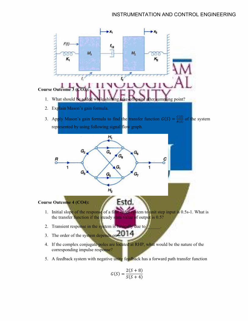
Course Outcome 3 (CO3):
1. What should be added while shifting take-off point after summing point?
2. Explain Mason’s gain formula.
3. Apply Mason’s gain formula to find the transfer function 𝐺(𝑆) =( )
( ) of the system
represented by using following signal flow graph.
Course Outcome 4 (CO4):
1. Initial slope of the response of a first order system to unit step input is 0.5s-1. What is the transfer function if the steady state value of output is 0.5?
2. Transient response in the system is basically due to ______.
3. The order of the system depends on ______.
4. If the complex conjugate poles are located at RHP, what would be the nature of the corresponding impulse response?
5. A feedback system with negative unity feedback has a forward path transfer function
𝐺(𝑆) =2(𝑆 + 8)
𝑆(𝑆 + 4)
INSTRUMENTATION AND CONTROL ENGINEERING
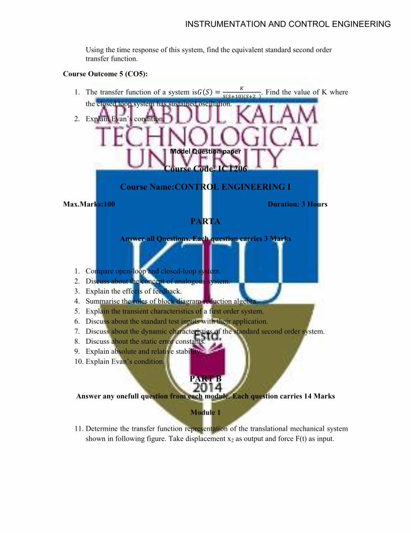
Using the time response of this system, find the equivalent standard second order transfer function.
Course Outcome 5 (CO5):
1. The transfer function of a system is𝐺(𝑆) =( )( )
. Find the value of K where
the closed loop system has sustained oscillation.
2. Explain Evan’s condition.
Model Question paper
Course Code: ICT206
Course Name:CONTROL ENGINEERING I
Max.Marks:100 Duration: 3 Hours
PARTA
Answer all Questions. Each question carries 3 Marks
1. Compare open-loop and closed-loop system. 2. Discuss about the concept of analogous system. 3. Explain the effects of feedback. 4. Summarise the rules of block diagram reduction algebra. 5. Explain the transient characteristics of a first order system. 6. Discuss about the standard test inputs with their application. 7. Discuss about the dynamic characteristics of the standard second order system. 8. Discuss about the static error constants. 9. Explain absolute and relative stability. 10. Explain Evan’s condition.
PART B
Answer any onefull question from each module. Each question carries 14 Marks
Module 1
11. Determine the transfer function representation of the translational mechanical system shown in following figure. Take displacement x2 as output and force F(t) as input.
INSTRUMENTATION AND CONTROL ENGINEERING
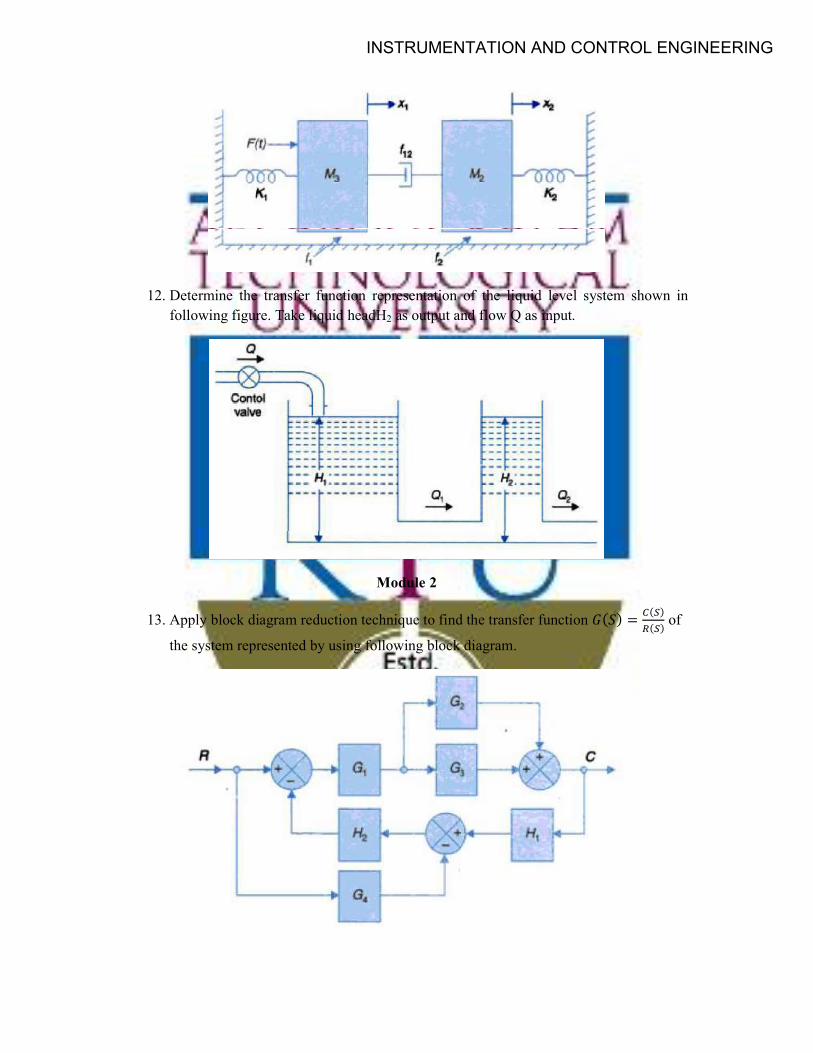
12. Determine the transfer function representation of the liquid level system shown in following figure. Take liquid headH2 as output and flow Q as input.
Module 2
13. Apply block diagram reduction technique to find the transfer function 𝐺(𝑆) =( )
( ) of
the system represented by using following block diagram.
INSTRUMENTATION AND CONTROL ENGINEERING
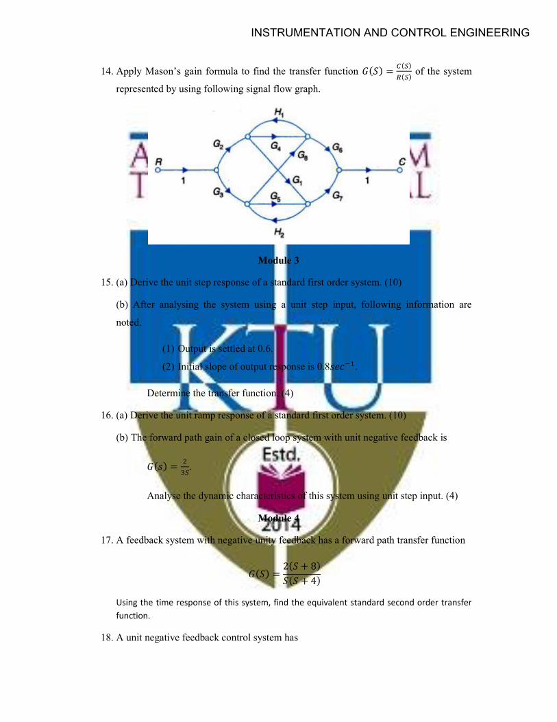
14. Apply Mason’s gain formula to find the transfer function 𝐺(𝑆) =( )
( ) of the system
represented by using following signal flow graph.
Module 3
15. (a) Derive the unit step response of a standard first order system. (10)
(b) After analysing the system using a unit step input, following information are
noted.
(1) Output is settled at 0.6.
(2) Initial slope of output response is 0.8𝑠𝑒𝑐 .
Determine the transfer function. (4)
16. (a) Derive the unit ramp response of a standard first order system. (10)
(b) The forward path gain of a closed loop system with unit negative feedback is
𝐺(𝑠) = .
Analyse the dynamic characteristics of this system using unit step input. (4)
Module 4
17. A feedback system with negative unity feedback has a forward path transfer function
𝐺(𝑆) =2(𝑆 + 8)
𝑆(𝑆 + 4)
Using the time response of this system, find the equivalent standard second order transfer function.
18. A unit negative feedback control system has
INSTRUMENTATION AND CONTROL ENGINEERING
𝐺(𝑆) =𝐾
𝑆 𝑆 + √2𝐾
(a) Determine the range of K where settling time of this system is less than 1 second. (5)
(b) Determine the dynamic characteristics of this system using the upper limit of K you got. (5)
(c) Determine the steady-state error of this system for a unit step and unit ramp input using the upper limit of K you got. (4)
Module 5
19. A system has a characteristic equation
𝑞(𝑆) = 𝑆 + 9𝑆 + 31.25𝑆 + 61.25𝑆 + 67.75𝑆 + 17.75𝑆 + 15 = 0
Determine whether the system is stable using Routh criteria.
20. Consider a system with forward path transfer function 𝐺(𝑆) =( )( )
and unit
negative feedback. Draw the root locus of the above system with respect to the variation of K from zero to infinity. Find the value of K at which the closed loop system is critically stable.
Syllabus
CONTROL ENGINEERING I
Module 1 (9 Hours)
Introduction to Control System
Introduction to control system; open-loop and closed loop systems; Feedback and non-feedback systems; servomechanism; history and development of automatic control.
Mathematical models of Physical Systems
Differential equation representation and transfer function representation; Differential equations and transfer functions of translational and rotational mechanical systems; Differential equations and transfer functions of electrical systems; Differential equations and transfer functions of thermal systems, fluid systems, and pneumatic systems; analogous systems; Transfer function of armature controlled dc motor and field controlled dc motor.
Module 2 (9 Hours)
INSTRUMENTATION AND CONTROL ENGINEERING
Block Diagram Algebra & Signal Flow Graphs
Block diagram of an open-loop system; Block diagram of a closed-loop system; block diagram and transfer function of a typical first order system, block diagram and transfer function of a typical second order system; block diagram of multi-input multi-output system; Block diagram reduction techniques; Concept of signal flow graph; construction of signal flow graph; Finding transfer function from Signal flow graph using Mason’s gain formula.
Feedback Characteristics of Control Systems
Reduction of parameter variation; control over system dynamics; control of the effects of disturbance signals.
Module 3 (8 Hours)
Time-domain Analysis of First-order Systems
Time response, transient and steady-state response; standard test signals and their application in system analysis; Open-loop and closed-loop transfer functions, type and order of systems; concept of poles and zeros; type and order of the system; Response of first order system to unit impulse, unit step and unit ramp input; Time response specifications of first order systems.
Module 4 (10 Hours)
Time-domain Analysis of Second-order Systems
Response of second order system (over damped, critically damped, and under damped) to unit step input; response of underdamped second order system to unit impulse and unit ramp input; Analysis of second order systems and time response specifications; poles of second order system and time response; Effect of adding a zero to a system.
Steady-state Errors and Error Constants
Steady-state response, steady state error, static and dynamic error coefficients.
Module 5 (9 Hours)
Stability of Linear Systems Stability of linear systems: Definitions, characteristic polynomial and characteristic equation, general stability criterion with reference to s-plane; Absolute and relative stability; necessary conditions for stability; Routh’s criterion of stability.
INSTRUMENTATION AND CONTROL ENGINEERING
The Root Locus Technique The root-locus concept; Evan’s criteria; Construction of root locus; determination of roots from root locus; Effect of addition of zeros and poles on root locus; root contours.
Text Books
1. I. J. Nagrath and M. Gopal, “Control Systems Engineering”, New Age International Pvt Ltd, 6/e.
2. Katsuhiko Ogata, “Modern Control Engineering”, Pearson Education India, 5/e.
3. Farid Golnaraghi and Benjamin C. Kuo, “Automatic Control Systems”, McGraw Hill Education (India) Pvt. Ltd., 10/e.
4. M. Gopal, “Control Systems Principles and Design”, McGraw Hill Education (India) Pvt. Ltd., 4/e.
5. A. Anand Kumar, “Control Systems”, PHI, 2/e.
6. D. Roy Choudhury, “Modern Control Engineering”, PHI.
7. K. Alice Mary and P. Ramana, “Control Systems”, Orient Black Swan.
Reference Books
1. Richard C. Dorf and Robert H. Bishop, “Modern Control Systems”, Pearson, 12/e.
2. Joseph J. Distefano III, Allen R. Stubberud & Ivan J. Williams, “Control Systems”, McGraw Hill Education (India) Pvt. Ltd., 3/e.
3. A. K. Jairath, “Control Systems with Essential Theory”, CBS Publishers and Distributors Pvt Ltd.
4. B. S. Manke, “Linear Control Systems with MATLAB Applications”, Khanna Publishers, 12/e.
5. D. Ganesh Rao & K. Chenna Venkatesh, “Control Engineering”, Cengage India Private Limited, 1/e.
6. Francis H. Raven, “Automatic Control Engineering”, McGraw Hill Education, 5/e.
7. Norman S. Nise, “Control Systems Engineering”, Wiley.
8. V. Krishnamurthi, “Control Systems”, CBS Publishers and Distributors Pvt Ltd, 1/e.
9. Prabir Kumar Sarkar, “Process Dynamics and Control”, PHI, 1/e.
10. A. Nagoor Kani, “Control Systems”, CBS Publishers and Distributors Pvt Ltd.
INSTRUMENTATION AND CONTROL ENGINEERING
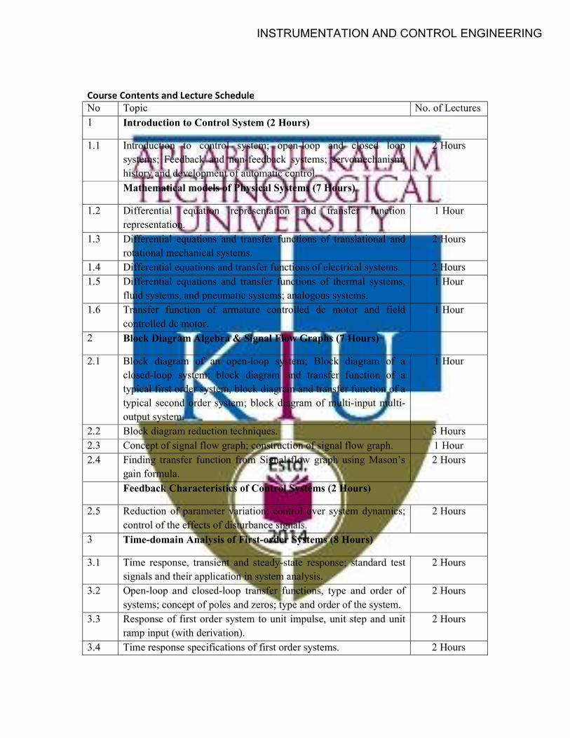
Course Contents and Lecture Schedule No Topic No. of Lectures 1 Introduction to Control System (2 Hours)
1.1 Introduction to control system; open-loop and closed loop systems; Feedback and non-feedback systems; servomechanism; history and development of automatic control.
2 Hours
Mathematical models of Physical Systems (7 Hours)
1.2 Differential equation representation and transfer function representation.
1 Hour
1.3 Differential equations and transfer functions of translational and rotational mechanical systems.
2 Hours
1.4 Differential equations and transfer functions of electrical systems. 2 Hours 1.5 Differential equations and transfer functions of thermal systems,
fluid systems, and pneumatic systems; analogous systems. 1 Hour
1.6 Transfer function of armature controlled dc motor and field controlled dc motor.
1 Hour
2 Block Diagram Algebra & Signal Flow Graphs (7 Hours)
2.1 Block diagram of an open-loop system; Block diagram of a closed-loop system; block diagram and transfer function of a typical first order system, block diagram and transfer function of a typical second order system; block diagram of multi-input multi-output system.
1 Hour
2.2 Block diagram reduction techniques. 3 Hours 2.3 Concept of signal flow graph; construction of signal flow graph. 1 Hour 2.4 Finding transfer function from Signal flow graph using Mason’s
gain formula. 2 Hours
Feedback Characteristics of Control Systems (2 Hours)
2.5 Reduction of parameter variation; control over system dynamics; control of the effects of disturbance signals.
2 Hours
3 Time-domain Analysis of First-order Systems (8 Hours)
3.1 Time response, transient and steady-state response; standard test signals and their application in system analysis.
2 Hours
3.2 Open-loop and closed-loop transfer functions, type and order of systems; concept of poles and zeros; type and order of the system.
2 Hours
3.3 Response of first order system to unit impulse, unit step and unit ramp input (with derivation).
2 Hours
3.4 Time response specifications of first order systems. 2 Hours
INSTRUMENTATION AND CONTROL ENGINEERING
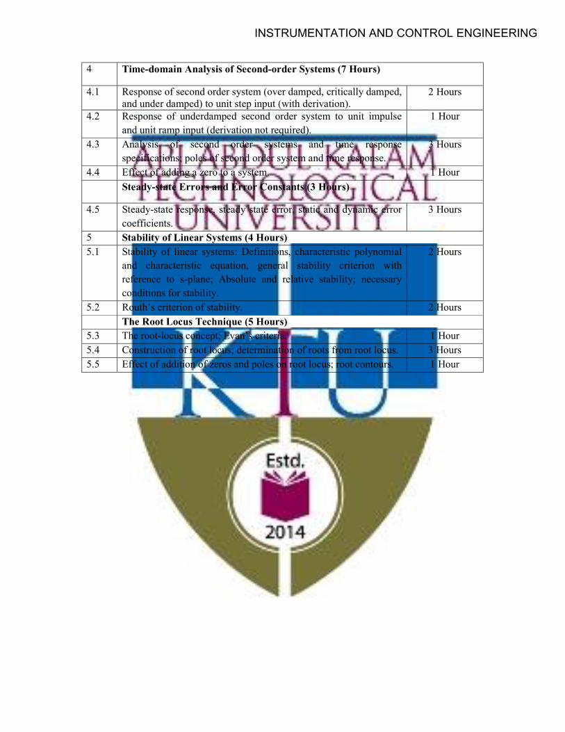
4 Time-domain Analysis of Second-order Systems (7 Hours)
4.1 Response of second order system (over damped, critically damped, and under damped) to unit step input (with derivation).
2 Hours
4.2 Response of underdamped second order system to unit impulse and unit ramp input (derivation not required).
1 Hour
4.3 Analysis of second order systems and time response specifications; poles of second order system and time response.
3 Hours
4.4 Effect of adding a zero to a system. 1 Hour Steady-state Errors and Error Constants (3 Hours)
4.5 Steady-state response, steady state error, static and dynamic error coefficients.
3 Hours
5 Stability of Linear Systems (4 Hours) 5.1 Stability of linear systems: Definitions, characteristic polynomial
and characteristic equation, general stability criterion with reference to s-plane; Absolute and relative stability; necessary conditions for stability.
2 Hours
5.2 Routh’s criterion of stability. 2 Hours The Root Locus Technique (5 Hours) 5.3 The root-locus concept; Evan’s criteria. 1 Hour 5.4 Construction of root locus; determination of roots from root locus. 3 Hours 5.5 Effect of addition of zeros and poles on root locus; root contours. 1 Hour
INSTRUMENTATION AND CONTROL ENGINEERING
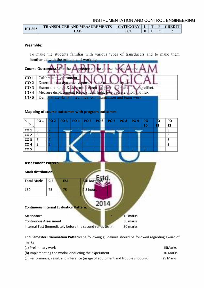
ICL202 TRANSDUCER AND MEASUREMENTS LAB
CATEGORY L T P CREDIT PCC 0 0 3 2
Preamble:
To make the students familiar with various types of transducers and to make them familiarize with the principle of working.
Course Outcomes:After the completion of the course the student are able to
CO 1 Calibrate an instrument. CO 2 Determine the dynamic response of a measurement system. CO 3 Extent the range & determine electrical parameters and loading effect. CO 4 Measure displacement, force, strain, light, level, acceleration and flux. CO 5 Demonstrate skills in technical communication and team work.
Mapping of course outcomes with program outcomes
PO 1 PO 2 PO 3 PO 4 PO 5 PO 6 PO 7 PO 8 PO 9 PO 10
PO 11
PO 12
CO 1 3 2 3 CO 2 3 2 3 CO 3 3 2 3 CO 4 3 2 3 CO 5 3 3
Assessment Pattern
Mark distribution
Total Marks CIE ESE ESE Duration
150 75 75 2.5 hours
Continuous Internal Evaluation Pattern:
Attendance : 15 marks Continuous Assessment : 30 marks Internal Test (Immediately before the second series test) : 30 marks End Semester Examination Pattern:The following guidelines should be followed regarding award of marks (a) Preliminary work : 15Marks (b) Implementing the work/Conducting the experiment : 10 Marks (c) Performance, result and inference (usage of equipment and trouble shooting) : 25 Marks
INSTRUMENTATION AND CONTROL ENGINEERING
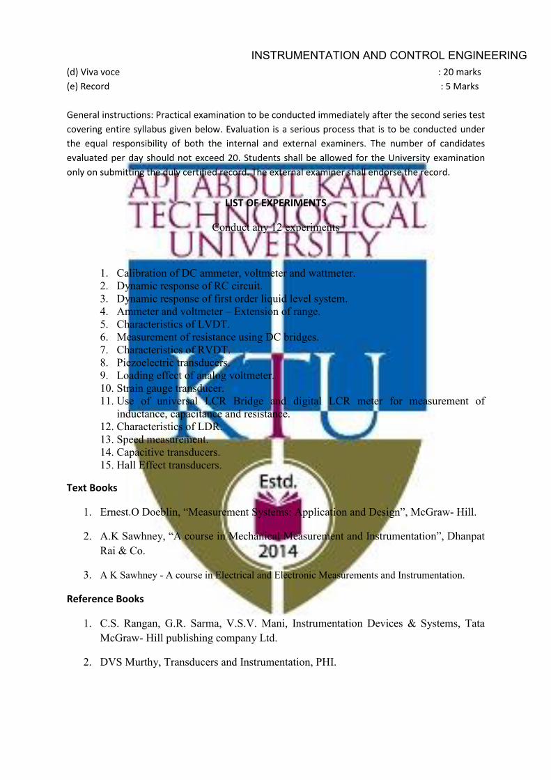
(d) Viva voce : 20 marks (e) Record : 5 Marks General instructions: Practical examination to be conducted immediately after the second series test covering entire syllabus given below. Evaluation is a serious process that is to be conducted under the equal responsibility of both the internal and external examiners. The number of candidates evaluated per day should not exceed 20. Students shall be allowed for the University examination only on submitting the duly certified record. The external examiner shall endorse the record.
LIST OF EXPERIMENTS
Conduct any 12 experiments
1. Calibration of DC ammeter, voltmeter and wattmeter. 2. Dynamic response of RC circuit. 3. Dynamic response of first order liquid level system. 4. Ammeter and voltmeter – Extension of range. 5. Characteristics of LVDT. 6. Measurement of resistance using DC bridges. 7. Characteristics of RVDT. 8. Piezoelectric transducers. 9. Loading effect of analog voltmeter. 10. Strain gauge transducer. 11. Use of universal LCR Bridge and digital LCR meter for measurement of
inductance, capacitance and resistance. 12. Characteristics of LDR. 13. Speed measurement. 14. Capacitive transducers. 15. Hall Effect transducers.
Text Books
1. Ernest.O Doeblin, “Measurement Systems: Application and Design”, McGraw- Hill.
2. A.K Sawhney, “A course in Mechanical Measurement and Instrumentation”, Dhanpat Rai & Co.
3. A K Sawhney - A course in Electrical and Electronic Measurements and Instrumentation.
Reference Books
1. C.S. Rangan, G.R. Sarma, V.S.V. Mani, Instrumentation Devices & Systems, Tata McGraw- Hill publishing company Ltd.
2. DVS Murthy, Transducers and Instrumentation, PHI.
INSTRUMENTATION AND CONTROL ENGINEERING
ICL204 ANALOG CIRCUITS LAB CATEGORY L T P CREDIT PCC 0 0 3 2
Preamble:
The lab is designed in order to get the students familiarized with the Integrated Circuits and to learn to design, set up and analyse circuits using active devices, op-amps and other ICs.
Prerequisite:
The lab is supposed to conduct in parallel with the theory subject ICT204-Integrated circuits and systems. Students are expected to study the topics covered in the theory class before coming to the respective lab experiment.
Course Outcomes:After the completion of the course the student will be able to
CO 1 Design the basic amplifiers and Estimate different offsets in op-amps. CO 2 Design various linear and non-linear circuits of op-amp. CO 3 Design and study the characteristics of different active filters. CO 4 Design different waveform generators, ADC and DAC. CO 5 Demonstrate skills in technical communication and team work.
Mapping of course outcomes with program outcomes
PO 1 PO 2 PO 3 PO 4 PO 5 PO 6 PO 7 PO 8 PO 9 PO 10
PO 11
PO 12
CO 1 3 3 CO 2 3 3 3 CO 3 3 3 3 3 CO 4 3 3 3 3 CO 5 3 3 2
Assessment Pattern
Mark distribution
Total Marks CIE ESE ESE Duration
150 75 75 2.5 hours
Continuous Internal Evaluation Pattern:
Attendance : 15 marks Continuous Assessment : 30 marks
INSTRUMENTATION AND CONTROL ENGINEERING
Internal Test (Immediately before the second series test) : 30 marks End Semester Examination Pattern:The following guidelines should be followed regarding award of marks (a) Preliminary work :15Marks (b) Implementing the work/Conducting the experiment :10 Marks (c) Performance, result and inference (usage of equipments and trouble shooting) : 25 Marks (d) Viva voce :20 marks (e) Record :5 Marks General instructions: Practical examination to be conducted immediately after the second series test covering entire syllabus given below. Evaluation is a serious process that is to be conducted under the equal responsibility of both the internal and external examiners. The number of candidates evaluated per day should not exceed 20. Students shall be allowed for the University examination only on submitting the duly certified record. The external examiner shall endorse the record.
LIST OF EXPERIMENTS (Minimum of 12 experiments mandatory)
1. Study of 741 op amp and implementation of basic circuits using 741 – Inverting, non-inverting, voltage follower.
2. Summing and difference amplifiers using op-amp. 3. Measurement of opamp parameters. 4. Instrumentation amplifier. 5. Active Integrator & differentiator circuits. 6. Comparator circuits using op-amp. 7. Active first and second order high pass & low pass filters. 8. Narrow Band pass filter. 9. Notch filter. 10. Wienbridge Oscillator. 11. Waveform generators (triangular & saw tooth). 12. Astablemultivibrator and Monostable multivibrator using opamp. 13. Astablemultivibrator and Monostable multivibrator using 555 timer. 14. Digital to analog converter (DAC). 15. Analog to digital converter (ADC). 16. Precision rectifiers.
Text Books
1. Ramakant A. Gayakwad, “Op-Amps and Linear Integrated Circuits”, Pearson Education Asia. 4/e.
2. D. Roy Choudhury, “Linear Integrated Circuits”, New Age International Publishers, 5/e.
INSTRUMENTATION AND CONTROL ENGINEERING

Reference Books
1. Robert L. Boylestad and Louis Nashelsky, “Electronic devices and circuit theory”, Pearson Education Asia. 11/e.
2. David A. Bell, ““Electronic devices and circuits”, Oxford, 5/e.
INSTRUMENTATION AND CONTROL ENGINEERING
SEMESTER -4
MINOR
INSTRUMENTATION AND CONTROL ENGINEERING
ICT282 LINEAR SYSTEM ANALYSIS CATEGORY L T P CREDIT
VAC 3 1 0 4
Preamble:
Aim of the course is to give an introduction about linear systems,its modelling using different tools and to analyse it in time domain.
Course Outcomes:
After the completion of the course the student will be able to
CO 1 Apply Laplace Transform method to analyse electrical networks.
CO 2 Explain about Z transform and its properties.
CO 3 Apply block diagram reduction techniques and Mason’s gain formula to reduce the systems represented by using block diagram and signal flow graph respectively.
CO 4 Analyse the linear time invariant system in time domain.
CO 5 Model and analyze systems in state variable form.
Mapping of course outcomes with program outcomes
PO 1 PO 2 PO 3 PO 4 PO 5 PO 6 PO 7 PO 8 PO 9 PO 10 PO 11 PO 12 CO 1 3 1 1 1 3 CO 2 3 3 CO 3 3 1 1 1 3 CO 4 3 1 1 1 3 CO 5 3 1 1 3
Assessment Pattern
Bloom’s Category Continuous Assessment Tests End Semester Examination 1 2
Remember Understand 10 10 20 Apply 30 30 60 Analyse 10 10 20 Evaluate Create
INSTRUMENTATION AND CONTROL ENGINEERING
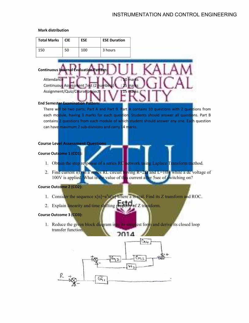
Mark distribution
Total Marks CIE ESE ESE Duration
150 50 100 3 hours
Continuous Internal Evaluation Pattern:
Attendance : 10 marks Continuous Assessment Test (2 numbers) : 25 marks Assignment/Quiz/Course project : 15 marks
End Semester Examination Pattern:
There will be two parts; Part A and Part B. Part A contains 10 questions with 2 questions from each module, having 3 marks for each question. Students should answer all questions. Part B contains 2 questions from each module of which student should answer any one. Each question can have maximum 2 sub-divisions and carry 14 marks.
Course Level Assessment Questions
Course Outcome 1 (CO1):
1. Obtain the step response of a series RC network using Laplace Transform method.
2. Find current i(t) in a series RL circuit having R=2Ω and L=10H while a dc voltage of 100V is applied. What is the value of this current after 5sec of switching on?
Course Outcome 2 (CO2):
1. Consider the sequence x[n]=anu[n] where a is real. Find its Z transform and ROC.
2. Explain linearity and time shifting property of Z transform.
Course Outcome 3 (CO3):
1. Reduce the given block diagram into its simplest form and derive its closed loop transfer function.
INSTRUMENTATION AND CONTROL ENGINEERING
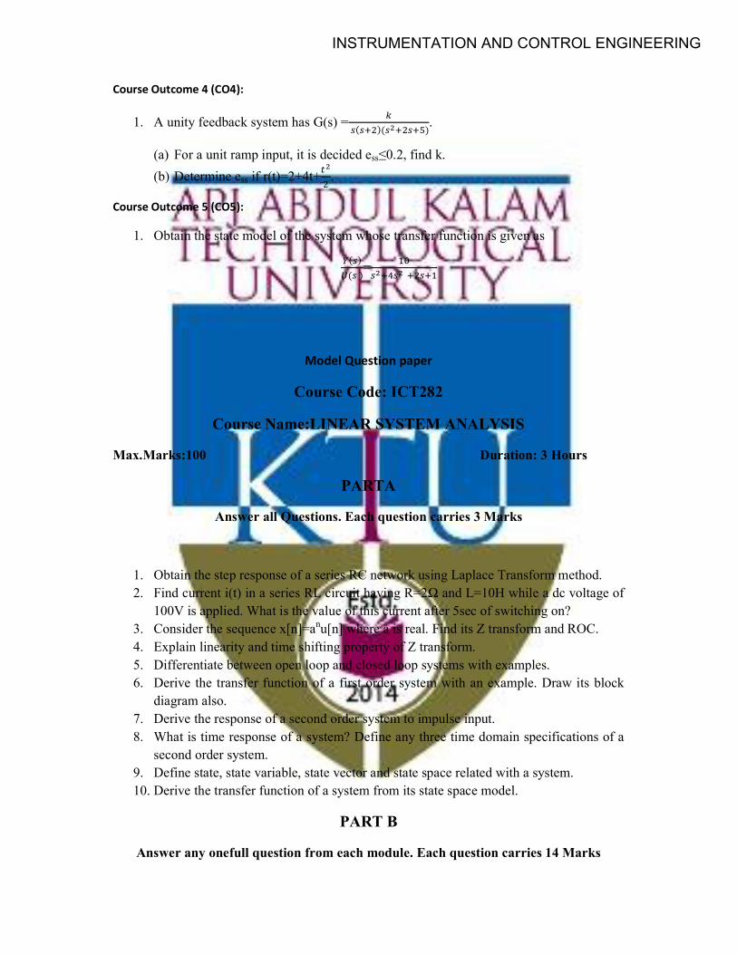
Course Outcome 4 (CO4):
1. A unity feedback system has G(s) = ( )( )
.
(a) For a unit ramp input, it is decided ess≤0.2, find k.
(b) Determine ess if r(t)=2+4t+ .
Course Outcome 5 (CO5):
1. Obtain the state model of the system whose transfer function is given as
( )
( )=
Model Question paper
Course Code: ICT282
Course Name:LINEAR SYSTEM ANALYSIS
Max.Marks:100 Duration: 3 Hours
PARTA
Answer all Questions. Each question carries 3 Marks
1. Obtain the step response of a series RC network using Laplace Transform method. 2. Find current i(t) in a series RL circuit having R=2Ω and L=10H while a dc voltage of
100V is applied. What is the value of this current after 5sec of switching on? 3. Consider the sequence x[n]=anu[n] where a is real. Find its Z transform and ROC. 4. Explain linearity and time shifting property of Z transform. 5. Differentiate between open loop and closed loop systems with examples. 6. Derive the transfer function of a first order system with an example. Draw its block
diagram also. 7. Derive the response of a second order system to impulse input. 8. What is time response of a system? Define any three time domain specifications of a
second order system. 9. Define state, state variable, state vector and state space related with a system. 10. Derive the transfer function of a system from its state space model.
PART B
Answer any onefull question from each module. Each question carries 14 Marks
INSTRUMENTATION AND CONTROL ENGINEERING
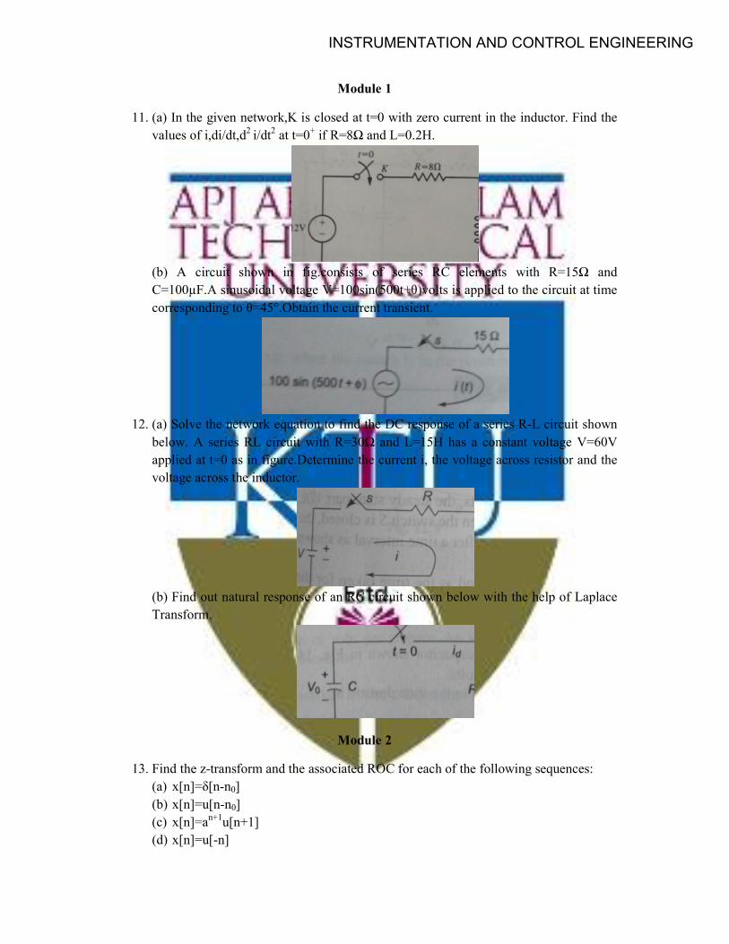
Module 1
11. (a) In the given network,K is closed at t=0 with zero current in the inductor. Find the values of i,di/dt,d2 i/dt2 at t=0+ if R=8Ω and L=0.2H.
(b) A circuit shown in fig.consists of series RC elements with R=15Ω and C=100µF.A sinusoidal voltage V=100sin(500t+θ)volts is applied to the circuit at time corresponding to θ=45°.Obtain the current transient.
12. (a) Solve the network equation to find the DC response of a series R-L circuit shown
below. A series RL circuit with R=30Ω and L=15H has a constant voltage V=60V applied at t=0 as in figure.Determine the current i, the voltage across resistor and the voltage across the inductor.
(b) Find out natural response of an RC circuit shown below with the help of Laplace Transform.
Module 2
13. Find the z-transform and the associated ROC for each of the following sequences: (a) x[n]=δ[n-n0] (b) x[n]=u[n-n0] (c) x[n]=an+1u[n+1] (d) x[n]=u[-n]
INSTRUMENTATION AND CONTROL ENGINEERING
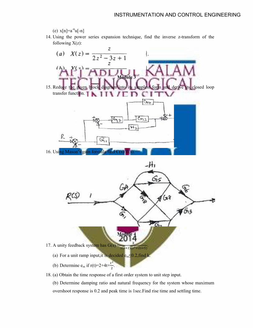
(e) x[n]=a-nu[-n] 14. Using the power series expansion technique, find the inverse z-transform of the
following X(z):
Module 3
15. Reduce the given block diagram into its simplest form and derive its closed loop transfer function.
16. Using Mason’s gain formula find C(s)/R(s).
Module 4
17. A unity feedback system has G(s) = ( )( )
.
(a) For a unit ramp input,it is decided ess≤0.2,find k.
(b) Determine ess if r(t)=2+4t+ .
18. (a) Obtain the time response of a first order system to unit step input.
(b) Determine damping ratio and natural frequency for the system whose maximum
overshoot response is 0.2 and peak time is 1sec.Find rise time and settling time.
INSTRUMENTATION AND CONTROL ENGINEERING
Module 5
19. Obtain the state model of the system whose transfer function is given as
( )
( )=
20. Determine the canonical state model of the system whose transfer function is T(s)=2(s+5)/[(s+2)(s+3)(s+4)]
Syllabus
LINEAR SYSTEM ANALYSIS
Module 1 (9 Hours)
LAPLACE TRANSFORM APPLICATIONS
Laplace Transform analysis of RL, RC and RLC networks. Transients- Review of transients in RC and RL networks with and significance of time constant- Initial conditions in the circuit elements of resistance, inductance and capacitance- Evaluation of initial condition- Initial state of a network- RLC network with internal excitation-Networks excited by external energy sources-DC, Sinusoidal and exponential inputs -Response as related to s-plane location of roots-General solutions in terms of ξ,ωn and Q.
Module 2 (9 Hours)
Z-TRANSFORMS
Fundamental difference between continuous and discrete time signals, concept of Z Transform of a discrete sequence, Region of convergence in Z-Transforms, properties of ROC,Z transforms of some common sequences(impulse, step), properties of Z-Transforms, The system function of discrete time LTI systems-System Function for LTI Systems Described by Linear Constant-Coefficient Difference Equations-characterization of discrete time LTI systems- systems interconnections –Unilateral Z transform-Inverse Z-Transform.
Module 3 (9 Hours)
INTRODUCTION TO CONTROL SYSTEM
Introduction to system modelling- open loop and closed loop systems-Differential equation model and Transfer function model - Block diagram representation – Block diagram and Transfer function of a typical first order system - Block diagram and transfer function of a typical second order system, Block diagram reduction techniques -Signal flow graphs – Masons’ gain formula.
INSTRUMENTATION AND CONTROL ENGINEERING
Module 4 (9 Hours)
TIME DOMAIN ANALYSIS
Time Domain Analysis -Time response – transient and steady state response. Standard test signals and their application in system analysis-Response of First order systems to impulse, step and ramp inputs -Response of second order systems to impulse, step and ramp inputs. Analysis of under damped second order system response to unit step input in detail – time domain specifications and their role in transient response- Steady state response – steady state error- static error co-efficient.
Module 5 (9 Hours)
STATE VARIABLE APPROACH
Concept of state, state variable, state vector and state space. State variable representation of continuous time systems using Physical variables. Transfer function from the state variable model- Transformation of state variables and invariance property-State variable model from transfer function – Bush or companion form – controllable canonical form–observable canonical form – Jordan canonical form. Diagonalization - state diagram.
Text Books
1. Van Valkenberg, “Network Analysis”, Pearson Education, 3/e.
2. Desoer C.A. & Kuh E.S., “Basic Circuit Theory”, McGraw Hill.
3. K. Ogata , “Modern Control Engineering”, Pearson Education India, 5/e.
4. Nagrath & Gopal, “Control System Engineering”, New Age International Pvt Ltd, 6/e.
5. Schaum’s outlines, “Signals and Systems”,McGraw Hill.
Reference Books
1. Ryder J.D., “Networks, Lines and Fields”, Prentice Hall India Learning Private Limited, 2/e.
2. Siskind, “Electrical Circuits”. McGraw Hill Text, 2/e.
3. Edminister, “Electric Circuits”, Schaum's Outline Series, McGraw Hill Education, 5/e.
4. Huelsman L.P., “Basic Circuit Theory”. Prentice Hall of India.
INSTRUMENTATION AND CONTROL ENGINEERING
5. B.C.Kuo, “Automatic Control System” , McGraw Hill Education, 1/e.
6. George.J. Thaler, “Automatic Control System”, Jaico Publishing House.
7. Gopal, “Digital Control and State Variable Methods”, McGraw Hill Education.
8. R.C. Dorf and R. H. Bishop, “Modem Control Systems” , Pearson Education.
Course Contents and Lecture Schedule No Topic No. of Lectures 1 Module I
1.1 Laplace Transform analysis of RL, RC and RLC networks 2 Hours
1.2 Transients- Review of transients in RC and RL networks with and significance of time constant
2 Hours
1.3 Initial conditions in the circuit elements of resistance, inductance and capacitance- Evaluation of initial condition- Initial state of a network-
2 Hours
1.4 RLC network with internal excitation. RC and RLC networks with external excitation, DC, Sinusoidal and exponential inputs- RLC circuits with DC excitation
3 Hours
2 Module II
2.1 Fundamental difference between continuous and discrete time signals, concept of Z Transform of a discrete sequence,
2 Hours
2.2 Region of convergence in Z-Transforms, properties of ROC 2 Hours
2.3 Z transforms of some common sequences (impulse, step),properties of Z-Transforms,
2 Hours
2.4 The system function of discrete time LTI systems-System Function for LTI Systems Described by Linear Constant-Coefficient DifferenceEquations-characterization of discrete time LTI systems-systems interconnections
2 Hours
2.5 Unilateral Z Transform-Inverse Z-Transform. 1 Hour
3 Module III
3.1 Introduction to system modelling- open loop and closed loop systems
1 Hour
3.2 Differential equation model and Transfer function model 2 Hours
3.3 Block diagram representation – Block diagram and Transfer function of a typical first order system - Block diagram and transfer function of a typical second order system
2 Hours
3.4 Block diagram reduction techniques - 2 Hours
3.5 Signal flow graphs – Masons’ gain formula 2 Hours
4 Module IV
INSTRUMENTATION AND CONTROL ENGINEERING
4.1 Time Domain Analysis -Time response – transient and steady state response. Standard test signals and their application in system analysis
1 Hour
4.2 Response of First order systems to impulse, step and ramp inputs -Response of second order systems to impulse, step and ramp inputs
2 Hours
4.3 Analysis of under damped second order system response to unit step input in detail
2 Hours
4.4 time domain specifications and their role in transient response 2 Hours
4.5 Steady state response – steady state error- static error co-efficient 2 Hours
5 Module V
5.1 Concept of state, state variable, state vector and state space 1 Hour
5.2 State variable representation of continuous time systems using Physical variables
1 Hour
5.3 Transfer function from the state variable model 2 Hours
5.4 Transformation of state variables and invariance property- State variable model from transfer function
2 Hours
5.5 Bush or companion form – controllable canonical form–observable canonical form – Jordan canonical form. Diagonalization - state diagram
3 Hours
INSTRUMENTATION AND CONTROL ENGINEERING
ICT284 INTRODUCTION TO VIRTUAL INSTRUMENTATION
CATEGORY L T P CREDIT VAC 3 1 0 4
Preamble:
The aim of the virtual instrumentationcourse is to make thestudents to obtain the knowledge of virtual instrumentation and some of its application. Virtual instrumentation combines mainstream commercial technologies, such as the PC, withflexible software and a wide variety of measurement hardware, so one can create user-defined virtual instrument systems that meet their exact application needs in instrumentation and control engineering field.
Prerequisite:
Course on basic electronics, electrical, instrumentation, op amps is required.
Course Outcomes:
After the completion of the course the student will be able to
CO 1 Define virtual instrumentation concepts and Compare traditional and virtual instrumentation.
CO 2 Study the basic building blocks of virtual instrumentation, usage of loops and arrays using LabVIEW.
CO 3 Study the usage of clusters and graphical indicators.
CO 4 Study the usage of structures, string operations and file operations.
CO 5 Study the instrument control and data acquisition using LabVIEW.
Mapping of course outcomes with program outcomes
PO 1 PO 2 PO 3 PO 4 PO 5 PO 6 PO 7 PO 8 PO 9 PO 10 PO 11 PO 12 CO 1 3 3 3 CO 2 3 3 3 CO 3 3 3 3 CO 4 3 3 3 CO 5 3 3 3
Assessment Pattern
Bloom’s Category Continuous Assessment Tests End Semester Examination 1 2
Remember 10 10 20
INSTRUMENTATION AND CONTROL ENGINEERING
Understand 20 20 40 Apply 20 20 40 Analyse Evaluate Create
Mark distribution
Total Marks CIE ESE ESE Duration
150 50 100 3 hours
Continuous Internal Evaluation Pattern:
Attendance : 10 marks Continuous Assessment Test (2 numbers) : 25 marks Assignment/Quiz/Course project : 15 marks *Assignment should be a miniproject.
End Semester Examination Pattern:
There will be two parts; Part A and Part B. Part A contains 10 questions with 2 questions from each module, having 3 marks for each question. Students should answer all questions. Part B contains 2 questions from each module of which student should answer any one. Each question can have maximum 2 sub-divisions and carry 14 marks.
Course Level Assessment Questions
Course Outcome 1 (CO1):
1. Differentiate virtual instrument and traditional instrument.
2. Differentiate graphical programming and textual programming.
Course Outcome 2 (CO2):
1. Write a note on global variables and local variables.
2. Explain polymorphism
Course Outcome 3 (CO3):
1. Explain the advantages of clusters over arrays.
2. Differentiate between XY graph and XY charts.
Course Outcome 4 (CO4):
1. Write a note on timed structures.
INSTRUMENTATION AND CONTROL ENGINEERING
2. Write a note onLabVIEW mathscript.
Course Outcome 5 (CO5):
1. Explain GPIB communication.
2. Explain DAQ software architecture.
Model Question paper
Course Code: ICT284
Course Name:INTRODUCTION TO VIRTUAL INSTRUMENTATION
Max.Marks:100 Duration: 3 Hours
PARTA
Answer all Questions. Each question carries 3 Marks
1. Define Virtual instrumentation. List any four merits of virtual instrumentation. 2. What is the use of Icon / connector pane? 3. Create a VI for converting Celsius to Fahrenheit. 4. Explain the difference between while loop for loop. 5. Distinguish Chart and graph. 6. Define clusters. What is the use of clusters? 7. Explain (1) Timed structures and (2) Event structures. 8. Explain (1) Formula Node and (2) Mathscript node. 9. Explain about DAQ Card and Point out the components of DAQ Cards. 10. Explain GPIB and Mention any two uses of GPIB.
PART B
Answer any onefull question from each module. Each question carries 14 Marks
Module 1
11. (a) With a neat diagram explain the layers of virtual instrumentation software and the software and hardware role. (7 Marks) (b) Explain controls and indicators in LabVIEW. (7 Marks)
12. (a) Discuss Virtual Instrumentation for Test, Control and Design. (5 Marks) (b) With figure, explain Graphical System Design Model. (5 Marks) (c) With Palettes, explain Front panel and Block diagram windows in LabVIEW. (4 Marks)
Module 2
INSTRUMENTATION AND CONTROL ENGINEERING
13. Write in detail about loops and charts. Explain them with an example. Explain in detail about local variables with examples.
14. (a) Define Module. Explain Modular Programming in LabVIEW. (7 Marks) (b) Explain arrays, array creation and array functions. (7 Marks)
Module 3
15. Explain clusters, cluster functions, controls and monitors. 16. Explain about the shift registers and feedback nodes with neat block diagram.
Module 4
17. Illustrate the operation of shift register showing the front panel and block diagram to
find the current count, previous count, count two iterations ago and count three
iterations ago and explain.
18. Develop a VI to check if a number is positive or negative. If yes, then the VI should
calculate and display the square root. Otherwise it should display a message and give
a value of -9999.00 as output. Solve using (1) case structure (2) select function and
(3) formula node.
Module 5
19. Explain the program architecture of GPIB code for devices simulator using
conventional VI’s with respect to that of VISA.
20. How VISA software interfaces permit the use of instruments under GPIB?
Syllabus
INTRODUCTION TO VIRTUAL INSTRUMENTATION
Module 1 (9 Hours)
Graphical system design
Graphical system design (GSD) model-design flow with GSD-virtual instrumentation-virtual instrument and traditional instrument-hardware and software in virtual instrumentation-virtual instrumentation for test, control and design-virtual instrumentation in the engineering process-virtual instruments beyond personal computer- graphical system design using LabVIEW-graphical programming and textual programming.
Introduction to LabVIEW
advantages of LabVIEW- software environment-creating and saving a vi -front panel toolbar- block diagram toolbar-palettes -shortcut menus - property dialog boxes - front panel controls
INSTRUMENTATION AND CONTROL ENGINEERING
and indicators- block diagram-data types -data flow program-LabVIEW documentation resources - keyboard shortcuts
Module 2 (10 Hours)
Modular programming
modular programming in LabVIEW - build a vi front panel and block diagram-icon and connector pane - creating an icon - building a connector pane- displaying subVIs and express vis as icons or expandable nodes - creating subVIs from sections of a vi - opening and editing subVIs - placing subVIs on block diagrams- saving subVIs - creating a stand-alone application.
Repetition and loops
For loops - while loops - structure tunnels- terminals inside or outside loops - shift registers-feedback nodes- control timing- communicating among multiple loops - local variables - global variables
Arrays
arrays in LabVIEW - creating one-dimensional array controls, indicators and constants - creating two-dimensional arrays-creating multidimensional arrays- initializing arrays - deleting elements, rows, columns and pages within arrays- inserting elements, rows, columns and pages into - replacing elements, rows, columns, and pages within arrays- array functions - auto indexing - creating two-dimensional arrays using loops - identification of data structure (scalar and array) using wires - using auto-indexing to set the for loop count - matrix operations with arrays-polymorphism.
Module 3 (8 Hours)
Clusters
Creating cluster controls and indicators- creating cluster constant - order of cluster elements - cluster operations - assembling clusters- disassembling clusters - conversion between arrays and clusters - error handling- error cluster.
Plotting data
types of waveforms - waveform graphs-waveform charts-waveform data type- XY graphs-intensity graphs and charts-digital waveform graphs-3d graphs - customizing graphs and charts-customizing graphs-customizing 3d graphs - customizing charts-dynamically formatting waveform graphs -configuring a graph or chart - displaying special planes on the XY graph.
INSTRUMENTATION AND CONTROL ENGINEERING
Module 4 (9 Hours)
Structures
Case structures-sequence structures-customizing structures- timed structures- formula nodes - event structure - LabVIEW mathscript.
Strings and file i/o
Creating string controls and indicators - string functions-editing, formatting and parsing strings - formatting strings - configuring string controls and indicators- basics of file input/output - choosing a file I/O format - LabVIEW data directory - file i/o VIs - creating a relative path.
Module 5 (9 Hours)
Instrument Control
Introduction - GPIB communication - hardware specifications - software architecture - instrument i/o assistant – visa- instrument - serial port communications - data transfer rate - serial port standards - using other interfaces.
Data acquisition
Transducers - signals- signal conditioning- DAQ hardware configuration - DAQ hardware - analog inputs - analog outputs - counters - digital I/O (DIO) – DAQ software architecture- DAQ assistant- channels and task configuration - selecting and configuring a data acquisition device- components of computer-based measurement system
Text Books
1. Jovitha Jerome, “Virtual Instrumentation using LabVIEW”, PHI Learning Pvt. Ltd, New Delhi.
2. Robert H. Bishop, “Learning with Lab-view”, Pearson, 2015.
3. S.Sumathi&P.Surekha, “LabVIEW based Advanced Instrumentation”, Springer, 2007.
Reference Books
1. Sanjay Gupta, Joseph John, “Virtual Instrumentation using LabVIEW”, McGraw Hill Education, 2/e.
INSTRUMENTATION AND CONTROL ENGINEERING
2. Gary W. Johnson, Richard Jennings, “LabVIEW Graphical Programming”, McGraw Hill Education, 4/e.
3. Gary Johnson, “Labview Graphical Programming”, McGraw-Hill Education, 4/e.
Course Contents and Lecture Schedule No Topic No. of Lectures 1 Graphical system design- (4 Hours)
1.1 Graphical system design (GSD) model-design flow with GSD- 1 Hour
1.2 Virtual instrumentation-virtual instrument and traditional instrument-hardware and software in virtual instrumentation-
1 Hour
1.3 Virtual instrumentation for test, control and design-virtual instrumentation in the engineering process-virtual instruments beyond personal computer- graphical system design using LabVIEW-graphical programming and textual programming.
2 Hours
Introduction to LabVIEW (5 Hours) 1.4 advantages of LabVIEW- software environment-creating and
saving a vi - 2 Hours
1.5 front panel toolbar- block diagram toolbar-palettes -shortcut menus - property dialog boxes - front panel controls and indicators- block diagram-data types -data flow program-LabVIEW documentation resources - keyboard shortcuts
3 Hours
2 Modular programming (2 Hrs) 2.1 modular programming in LabVIEW - build a vi front panel and
block diagram-icon and connector pane - creating an icon - building a connector pane- displaying subVIs and express vis as icons or expandable nodes -
1 Hour
2.2 Creating subVIs from sections of a vi - opening and editing subVIs - placing subVIs on block diagrams- saving subVIs - creating a stand-alone application.
1 Hour
Repetition and loops (4 Hrs) 2.3 for loops - while loops - structure tunnels- terminals inside or
outside loops - 2 Hours
2.4 shift registers-feedback nodes- control timing- communicating among multiple loops - local variables - global variables
2 Hours
Arrays(4 Hrs) 2.5 arrays in LabVIEW - creating one-dimensional array controls, 3 Hours
INSTRUMENTATION AND CONTROL ENGINEERING
indicatorsand constants - creating two-dimensional arrays-creating multidimensional arrays- initializing arrays - deleting elements, rows, columns and pages within arrays- inserting elements, rows, columns and pages into - replacing elements, rows, columns, and pageswithin arrays- array functions - auto indexing -
2.6 Creating two-dimensional arrays using loops - identification of data structure (scalar and array)using wires - using auto-indexing to set the for loop count - matrix operations with arrays-polymorphism.
1 Hour
3 Clusters (4 Hours) 3.1 creating cluster controls and indicators- creating cluster constant
- order of cluster elements - cluster operations - 1 Hour
3.2 Assembling clusters- disassembling clusters - conversion between arrays and clusters - error handling- error cluster.
3 Hours
Plotting data (4 Hours) 3.3 types of waveforms - waveform graphs-waveform charts-
waveform data type- XY graphs-intensity graphs and charts-digital waveform graphs-
2 Hours
3.4 3d graphs - customizing graphs and charts-customizing graphs-customizing 3d graphs - customizing charts-dynamically formatting waveform graphs -configuring a graph or chart - displaying special planes on the XY graph.
2Hours
4 Structures (4 Hours) 4.1 case structures-sequence structures-customizing structures- 1 Hour 4.2 Timed structures- formula nodes - event structure - LabVIEW
mathscript. 3 Hours
Strings and file i/o (5 Hours) 4.3 - creating string controls and indicators - string functions-
editing, formatting and parsing strings - formatting strings - configuring string controls and indicators-
2 Hours
4.4 Basics of file input/output - choosing a file I/O format - LabVIEW data directory - file i/o VIs - creating a relative path.
3 Hours
5 Instrument Control (4 Hours)
5.1 introduction - GPIB communication - hardware specifications - software architecture - instrument i/o assistant –
1 Hour
5.2 Visa- instrument - serial port communications - data transfer rate - serial port standards - using other interfaces.
3 Hours
Data acquisition (5 Hours)
INSTRUMENTATION AND CONTROL ENGINEERING
5.3 Transducers - signals- signal conditioning- DAQ hardware configuration - DAQ hardware - analog inputs - analog outputs -
3 Hours
5.4 counters - digital I/O (DIO) – DAQ software architecture- DAQ assistant- channels and task configuration -
1 Hour
5.5 selecting and configuring a data acquisition device- components of computer-based measurement system
1 Hour
INSTRUMENTATION AND CONTROL ENGINEERING
SEMESTER -4
HONOURS
INSTRUMENTATION AND CONTROL ENGINEERING
ICT292 ENGINEERING OPTIMIZATION CATEGORY L T P CREDIT VAC 3 1 0 4
Preamble:
The aim of the Engineering Optimization course is to offer students the fundaments techniques used to find the optimal solution of engineering problems.
Prerequisite:
Mathematics course in differential equations, linear algebra, and computational techniques.
Course Outcomes:
After the completion of the course the student will be able to
CO 1 Apply classical optimization techniques to constrained and unconstrained engineering optimization problems.
CO 2 Apply simplex method to find the solution of linear optimization problems.
CO 3 Solve unconstrained optimization problems by using direct search techniques.
CO 4 Solve unconstrained optimization problems by using descent techniques.
CO 5 Solve constrained optimization problems by using direct search techniques.
Mapping of course outcomes with program outcomes
PO 1 PO 2 PO 3 PO 4 PO 5 PO 6 PO 7 PO 8 PO 9 PO 10 PO 11 PO 12 CO 1 3 2 3 3 CO 2 3 2 3 3 CO 3 3 2 3 3 CO 4 3 2 3 3 CO 5 3 2 3 3
Assessment Pattern
Bloom’s Category Continuous Assessment Tests End Semester Examination 1 2
Remember Understand 15 15 30 Apply 35 35 70 Analyse Evaluate Create
INSTRUMENTATION AND CONTROL ENGINEERING
Mark distribution
Total Marks CIE ESE ESE Duration
150 50 100 3 hours
Continuous Internal Evaluation Pattern:
Attendance : 10 marks Continuous Assessment Test (2 numbers) : 25 marks Assignment/Quiz/Course project : 15 marks
End Semester Examination Pattern:
There will be two parts; Part A and Part B. Part A contains 10 questions with 2 questions from each module, having 3 marks for each question. Students should answer all questions. Part B contains 2 questions from each module of which student should answer any one. Each question can have maximum 2 sub-divisions and carry 14 marks.
Course Level Assessment Questions
Course Outcome 1 (CO1):
1. In a two-stage compressor, the working gas leaving the first stage of compression is cooled before it enters the second stage of compression to increase the efficiency. The total work input to a compressor (W) for an ideal gas, for isentropic compression, is given by
𝑊𝑊 = 𝐶𝐶𝑃𝑃𝑇𝑇1 𝑃𝑃2
𝑃𝑃1𝑘𝑘−1
𝑘𝑘
+ 𝑃𝑃3
𝑃𝑃2𝑘𝑘−1
𝑘𝑘
− 2
where 𝐶𝐶𝑃𝑃 is the specific heat of the gas at constant pressure, k is the ratio of specific heat at constant pressure to that at constant volume of the gas, and 𝑇𝑇1 is the temperature at which the gas enters the compressor. Find the pressure, 𝑝𝑝2 at which intercooling should be done to minimize the work input to the compressor. Also determine the minimum work done on the compressor.
Course Outcome 2 (CO2):
1. Find all the basic solutions corresponding to the system of equations 2𝑥𝑥1 + 3𝑥𝑥2 − 2𝑥𝑥3 − 7𝑥𝑥4 = 1 𝑥𝑥1 + 𝑥𝑥2 + 𝑥𝑥3 + 3𝑥𝑥4 = 6 𝑥𝑥1 − 𝑥𝑥2 + 𝑥𝑥3 + 5𝑥𝑥4 = 4
Course Outcome 3 (CO3):
INSTRUMENTATION AND CONTROL ENGINEERING
1. Minimize 𝑓𝑓(𝑥𝑥1, 𝑥𝑥2) = 𝑥𝑥1 − 𝑥𝑥2 + 2𝑥𝑥12 + 2𝑥𝑥1𝑥𝑥2 + 𝑥𝑥2
2 with the starting point (0,0) using any one direct search method.
Course Outcome 4 (CO4):
1. Minimize 𝑓𝑓(𝑥𝑥1, 𝑥𝑥2) = 𝑥𝑥1 − 𝑥𝑥2 + 2𝑥𝑥12 + 2𝑥𝑥1𝑥𝑥2 + 𝑥𝑥2
2 with the starting point (0,0) using any one descent method.
Course Outcome 5 (CO5):
1. Minimize 𝑓𝑓(𝑥𝑥1, 𝑥𝑥2) = 𝑥𝑥12 + 𝑥𝑥2
2 − 2𝑥𝑥1 − 4𝑥𝑥2 subject to 𝑔𝑔1(𝑥𝑥1,𝑥𝑥2) = 𝑥𝑥1 + 4𝑥𝑥2 − 5 ≤ 0; 𝑔𝑔2(𝑥𝑥1, 𝑥𝑥2) = 2𝑥𝑥1 + 3𝑥𝑥2 − 6 ≤ 0; 𝑔𝑔3(𝑥𝑥1, 𝑥𝑥2) = −𝑥𝑥1 ≤ 0; 𝑔𝑔4(𝑥𝑥1, 𝑥𝑥2) = −𝑥𝑥2 ≤ 0 starting from point (1,1) using any one direct search method.
Model Question paper
Course Code: ICT292
Course Name:ENGINEERING OPTIMIZATION
Max.Marks:100 Duration: 3 Hours
PARTA
Answer all Questions. Each question carries 3 Marks
1. State and prove the necessary and sufficient conditions for the relative minimum of a function of a single variable.
2. Explain saddle point. 3. What is convex set? Explain. 4. Explain pivot operation. 5. State the necessary and sufficient conditions for the unconstrained minimum of a
function. 6. Give three reasons why the study of unconstrained minimization methods is
important. 7. Why is the steepest descent direction not efficient in practice, although the directions
used are the best directions? Explain. 8. Why is the DFP method considered as a variable metric method? Explain. 9. Explain the features of constrained optimization. 10. Formulate the equivalent unconstrained objective function that can be used in random
search methods.
PART B
INSTRUMENTATION AND CONTROL ENGINEERING
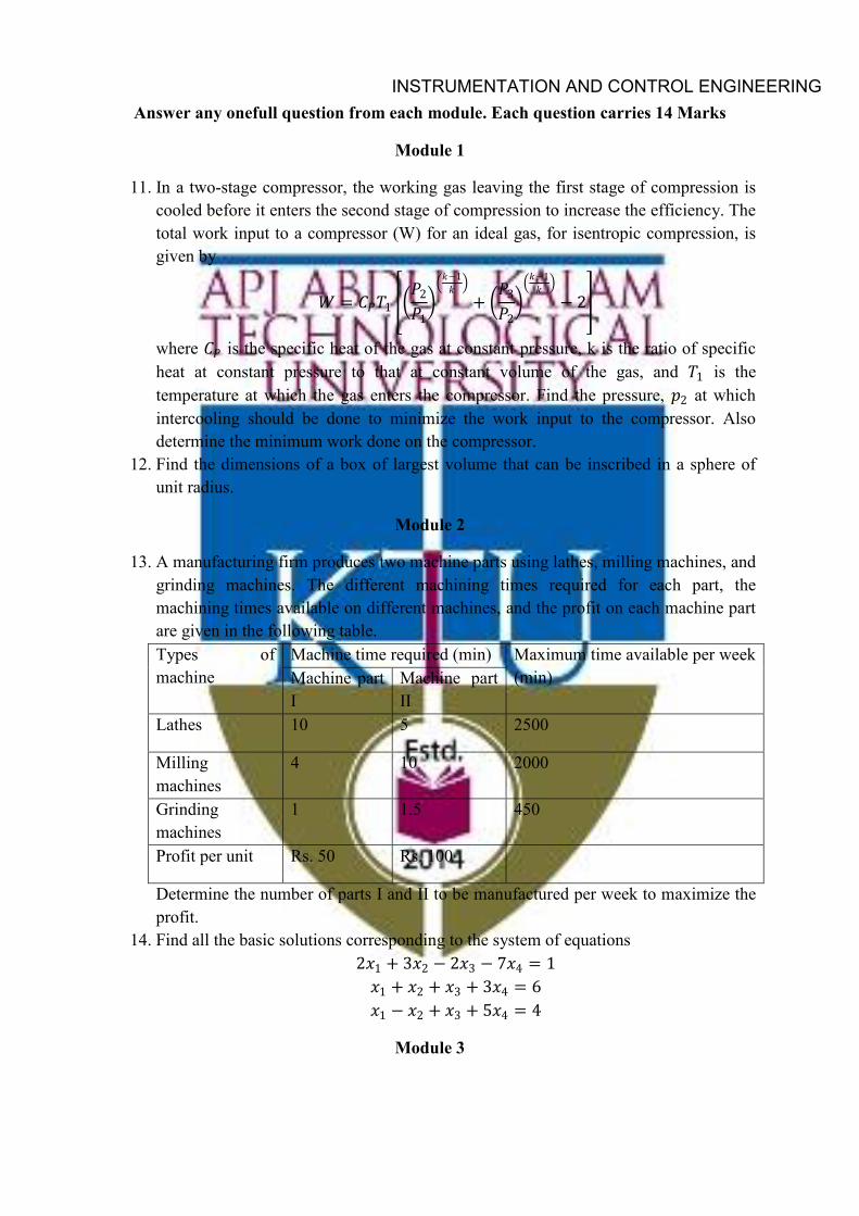
Answer any onefull question from each module. Each question carries 14 Marks
Module 1
11. In a two-stage compressor, the working gas leaving the first stage of compression is cooled before it enters the second stage of compression to increase the efficiency. The total work input to a compressor (W) for an ideal gas, for isentropic compression, is given by
𝑊𝑊 = 𝐶𝐶𝑃𝑃𝑇𝑇1 𝑃𝑃2
𝑃𝑃1𝑘𝑘−1
𝑘𝑘
+ 𝑃𝑃3
𝑃𝑃2𝑘𝑘−1
𝑘𝑘
− 2
where 𝐶𝐶𝑃𝑃 is the specific heat of the gas at constant pressure, k is the ratio of specific heat at constant pressure to that at constant volume of the gas, and 𝑇𝑇1 is the temperature at which the gas enters the compressor. Find the pressure, 𝑝𝑝2 at which intercooling should be done to minimize the work input to the compressor. Also determine the minimum work done on the compressor.
12. Find the dimensions of a box of largest volume that can be inscribed in a sphere of unit radius.
Module 2
13. A manufacturing firm produces two machine parts using lathes, milling machines, and grinding machines. The different machining times required for each part, the machining times available on different machines, and the profit on each machine part are given in the following table. Types of machine
Machine time required (min) Maximum time available per week (min) Machine part
I Machine part II
Lathes 10 5 2500
Milling machines
4 10 2000
Grinding machines
1 1.5 450
Profit per unit Rs. 50 Rs. 100
Determine the number of parts I and II to be manufactured per week to maximize the profit.
14. Find all the basic solutions corresponding to the system of equations 2𝑥𝑥1 + 3𝑥𝑥2 − 2𝑥𝑥3 − 7𝑥𝑥4 = 1 𝑥𝑥1 + 𝑥𝑥2 + 𝑥𝑥3 + 3𝑥𝑥4 = 6 𝑥𝑥1 − 𝑥𝑥2 + 𝑥𝑥3 + 5𝑥𝑥4 = 4
Module 3
INSTRUMENTATION AND CONTROL ENGINEERING
15. Minimize 𝑓𝑓(𝑥𝑥1, 𝑥𝑥2) = 𝑥𝑥1 − 𝑥𝑥2 + 2𝑥𝑥12 + 2𝑥𝑥1𝑥𝑥2 + 𝑥𝑥2
2 with the starting point (0,0) using any one direct search method.
16. Consider the problem: 𝑓𝑓 = 100(𝑥𝑥2 − 𝑥𝑥1
2)2 + (1 − 𝑥𝑥1)2 Find the solution of the problem using grid search with a step size ∆𝑥𝑥𝑖𝑖 = 0.1 in the range −3 ≤ 𝑥𝑥𝑖𝑖 ≤ 3, 𝑖𝑖 = 1,2.
Module 4
17. Minimize 𝑓𝑓(𝑥𝑥1, 𝑥𝑥2) = 𝑥𝑥1 − 𝑥𝑥2 + 2𝑥𝑥12 + 2𝑥𝑥1𝑥𝑥2 + 𝑥𝑥2
2 with the starting point (0,0) using
any one descent method.
18. Show that DFP method is a conjugate gradient method.
Module 5
19. Minimize 𝑓𝑓(𝑥𝑥1, 𝑥𝑥2) = 𝑥𝑥1 − 𝑥𝑥2 subject to 3𝑥𝑥12 − 2𝑥𝑥1𝑥𝑥2 + 𝑥𝑥2
2 − 1 ≤ 0 using the
cutting plane method. Take he convergence limit in step 5 as ∈= 0.02.
20. Minimize 𝑓𝑓(𝑥𝑥1, 𝑥𝑥2) = 𝑥𝑥12 + 𝑥𝑥2
2 − 2𝑥𝑥1 − 4𝑥𝑥2 subject to 𝑔𝑔1(𝑥𝑥1,𝑥𝑥2) = 𝑥𝑥1 + 4𝑥𝑥2 − 5 ≤ 0; 𝑔𝑔2(𝑥𝑥1, 𝑥𝑥2) = 2𝑥𝑥1 + 3𝑥𝑥2 − 6 ≤ 0; 𝑔𝑔3(𝑥𝑥1, 𝑥𝑥2) = −𝑥𝑥1 ≤ 0; 𝑔𝑔4(𝑥𝑥1, 𝑥𝑥2) = −𝑥𝑥2 ≤ 0 starting from point (1,1) using any one direct search method.
Syllabus
ENGINEERING OPTIMIZATION
Module 1 (9 Hours)
Introduction to Optimization
Introduction; engineering applications of optimization; statement of an optimization problem: design vector, design constraints, constraint surface, objective function, and objective function surface; classification of optimization problems: classification based on the existence of constraints, classification based on the nature of the design variables, classification based on the basic structure of the problem, classification based on the nature of the equations involved, classification based on the permissible values of the design variables, classification based on the deterministic nature of the variables, classification based on the separability of the functions, classification based on the number of objective functions; optimization techniques.
Classical Optimization Techniques
Single variable optimization; multi variable optimization with no constraints: semi definite case, saddle point; Multivariable optimization with equality constraints: solution by direct
INSTRUMENTATION AND CONTROL ENGINEERING
substitution, solution by the method of constrained variation, solution by the method of Lagrange multipliers; Multi variable optimization with inequality constraints: Kuhn Tucker conditions, constraint qualification; convex programming problem.
Module 2 (9 Hours)
Simplex Method
Application of linear programming; standard form of a linear programming problem; geometry of linear programming problems; Definitions and theorems; Solution of a system of linear simultaneous equations; pivotal reduction of a general system of equations; motivation of the simplex method; simplex algorithm; Two phases of the simplex method; duality of linear programming; Decomposition principle.
Module 3 (8 Hours)
Unconstrained Optimization Techniques using Direct Search Methods
Classifications of unconstrained minimization methods; Random search methods: Random jumping method, and random walk method; grid search method; univariate method; pattern direction; Hooke and Jeeves method; Powell’s method: conjugate directions, algorithms; Simplex method: reflection, expansion, contraction.
Module 4 (10 Hours)
Unconstrained Optimization Techniques using Descent Methods
Gradient of a function: evaluation of the gradient; steepest descent method; Conjugate gradient method: development; Newton’s method; Marquardt method; Quasi-Newton method; Davidon-Fletcher-Powell method; Broyden-Fletcher-Goldfarb-Shanno method; test functions.
Module 5 (9 Hours)
Constrained Optimization Techniques using Direct Search Methods Characteristics of constrained problem; random search methods; complex method; sequential linear programming; Basic approach in the methods of feasible directions; Zoutendijk’s method of feasible directions: direction-finding problems, determination step length, termination criteria; Rosen’s gradient projection method: determination of step length; generalized reduced gradient method; sequential quadratic programming.
INSTRUMENTATION AND CONTROL ENGINEERING
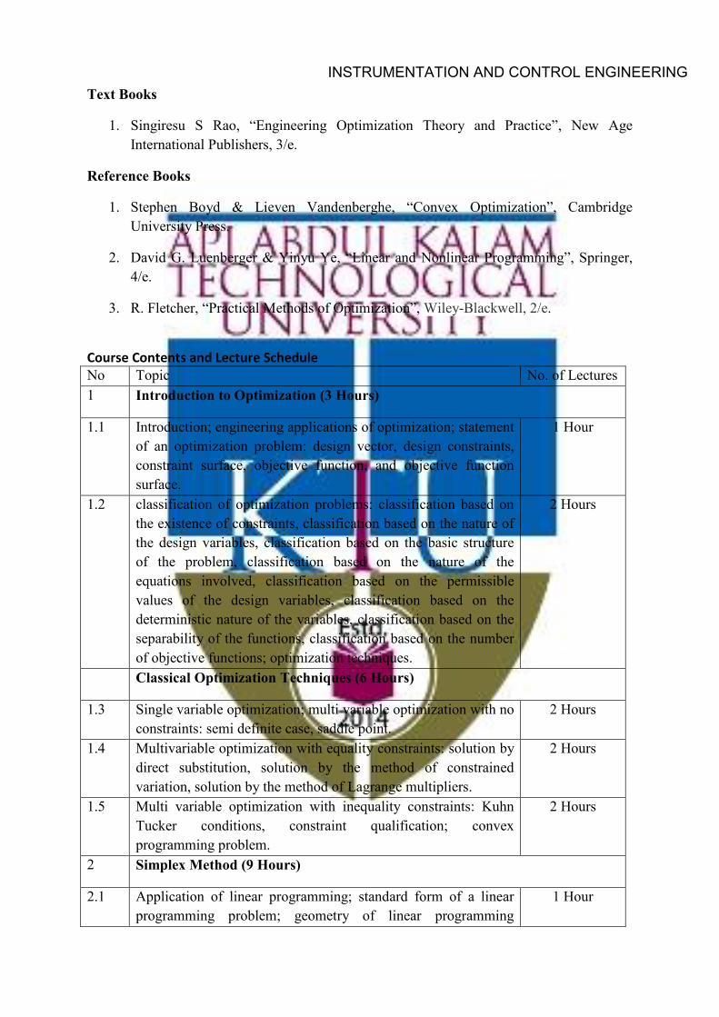
Text Books
1. Singiresu S Rao, “Engineering Optimization Theory and Practice”, New Age International Publishers, 3/e.
Reference Books
1. Stephen Boyd & Lieven Vandenberghe, “Convex Optimization”, Cambridge University Press.
2. David G. Luenberger & Yinyu Ye, “Linear and Nonlinear Programming”, Springer, 4/e.
3. R. Fletcher, “Practical Methods of Optimization”, Wiley-Blackwell, 2/e.
Course Contents and Lecture Schedule No Topic No. of Lectures 1 Introduction to Optimization (3 Hours)
1.1 Introduction; engineering applications of optimization; statement of an optimization problem: design vector, design constraints, constraint surface, objective function, and objective function surface.
1 Hour
1.2 classification of optimization problems: classification based on the existence of constraints, classification based on the nature of the design variables, classification based on the basic structure of the problem, classification based on the nature of the equations involved, classification based on the permissible values of the design variables, classification based on the deterministic nature of the variables, classification based on the separability of the functions, classification based on the number of objective functions; optimization techniques.
2 Hours
Classical Optimization Techniques (6 Hours)
1.3 Single variable optimization; multi variable optimization with no constraints: semi definite case, saddle point.
2 Hours
1.4 Multivariable optimization with equality constraints: solution by direct substitution, solution by the method of constrained variation, solution by the method of Lagrange multipliers.
2 Hours
1.5 Multi variable optimization with inequality constraints: Kuhn Tucker conditions, constraint qualification; convex programming problem.
2 Hours
2 Simplex Method (9 Hours)
2.1 Application of linear programming; standard form of a linear programming problem; geometry of linear programming
1 Hour
INSTRUMENTATION AND CONTROL ENGINEERING
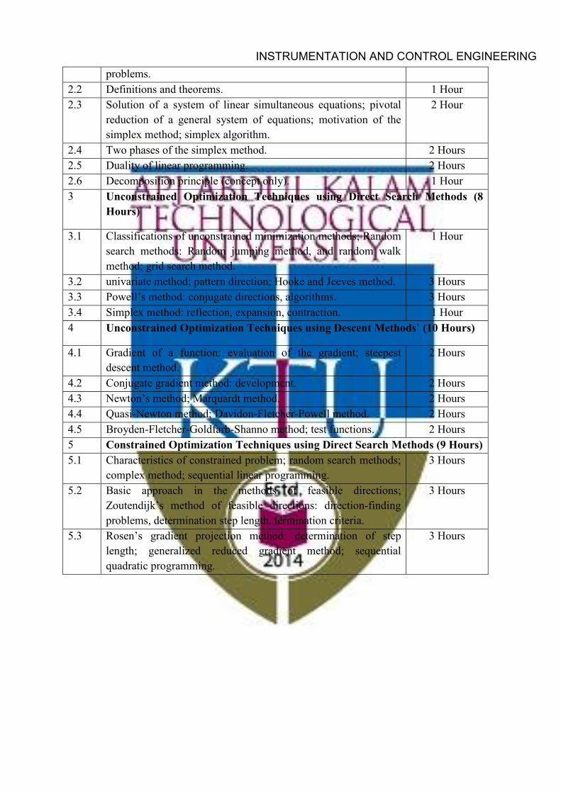
problems. 2.2 Definitions and theorems. 1 Hour 2.3 Solution of a system of linear simultaneous equations; pivotal
reduction of a general system of equations; motivation of the simplex method; simplex algorithm.
2 Hour
2.4 Two phases of the simplex method. 2 Hours 2.5 Duality of linear programming. 2 Hours 2.6 Decomposition principle (concept only). 1 Hour 3 Unconstrained Optimization Techniques using Direct Search Methods (8
Hours)
3.1 Classifications of unconstrained minimization methods; Random search methods: Random jumping method, and random walk method; grid search method.
1 Hour
3.2 univariate method; pattern direction; Hooke and Jeeves method. 3 Hours 3.3 Powell’s method: conjugate directions, algorithms. 3 Hours 3.4 Simplex method: reflection, expansion, contraction. 1 Hour 4 Unconstrained Optimization Techniques using Descent Methods` (10 Hours)
4.1 Gradient of a function: evaluation of the gradient; steepest descent method.
2 Hours
4.2 Conjugate gradient method: development. 2 Hours 4.3 Newton’s method; Marquardt method. 2 Hours 4.4 Quasi-Newton method; Davidon-Fletcher-Powell method. 2 Hours 4.5 Broyden-Fletcher-Goldfarb-Shanno method; test functions. 2 Hours 5 Constrained Optimization Techniques using Direct Search Methods (9 Hours) 5.1 Characteristics of constrained problem; random search methods;
complex method; sequential linear programming. 3 Hours
5.2 Basic approach in the methods of feasible directions; Zoutendijk’s method of feasible directions: direction-finding problems, determination step length, termination criteria.
3 Hours
5.3 Rosen’s gradient projection method: determination of step length; generalized reduced gradient method; sequential quadratic programming.
3 Hours
INSTRUMENTATION AND CONTROL ENGINEERING
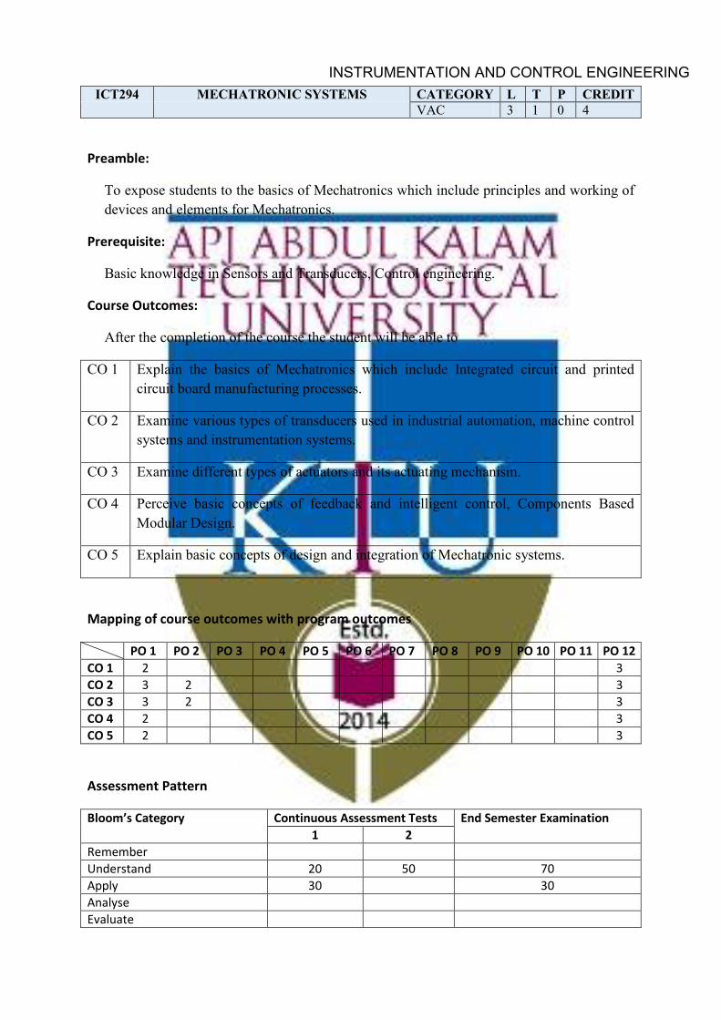
ICT294 MECHATRONIC SYSTEMS CATEGORY L T P CREDIT VAC 3 1 0 4
Preamble:
To expose students to the basics of Mechatronics which include principles and working of devices and elements for Mechatronics.
Prerequisite:
Basic knowledge in Sensors and Transducers, Control engineering.
Course Outcomes:
After the completion of the course the student will be able to
CO 1 Explain the basics of Mechatronics which include Integrated circuit and printed circuit board manufacturing processes.
CO 2 Examine various types of transducers used in industrial automation, machine control systems and instrumentation systems.
CO 3 Examine different types of actuators and its actuating mechanism.
CO 4 Perceive basic concepts of feedback and intelligent control, Components Based Modular Design.
CO 5 Explain basic concepts of design and integration of Mechatronic systems.
Mapping of course outcomes with program outcomes
PO 1 PO 2 PO 3 PO 4 PO 5 PO 6 PO 7 PO 8 PO 9 PO 10 PO 11 PO 12 CO 1 2 3 CO 2 3 2 3 CO 3 3 2 3 CO 4 2 3 CO 5 2 3
Assessment Pattern
Bloom’s Category Continuous Assessment Tests End Semester Examination 1 2
Remember Understand 20 50 70 Apply 30 30 Analyse Evaluate
INSTRUMENTATION AND CONTROL ENGINEERING
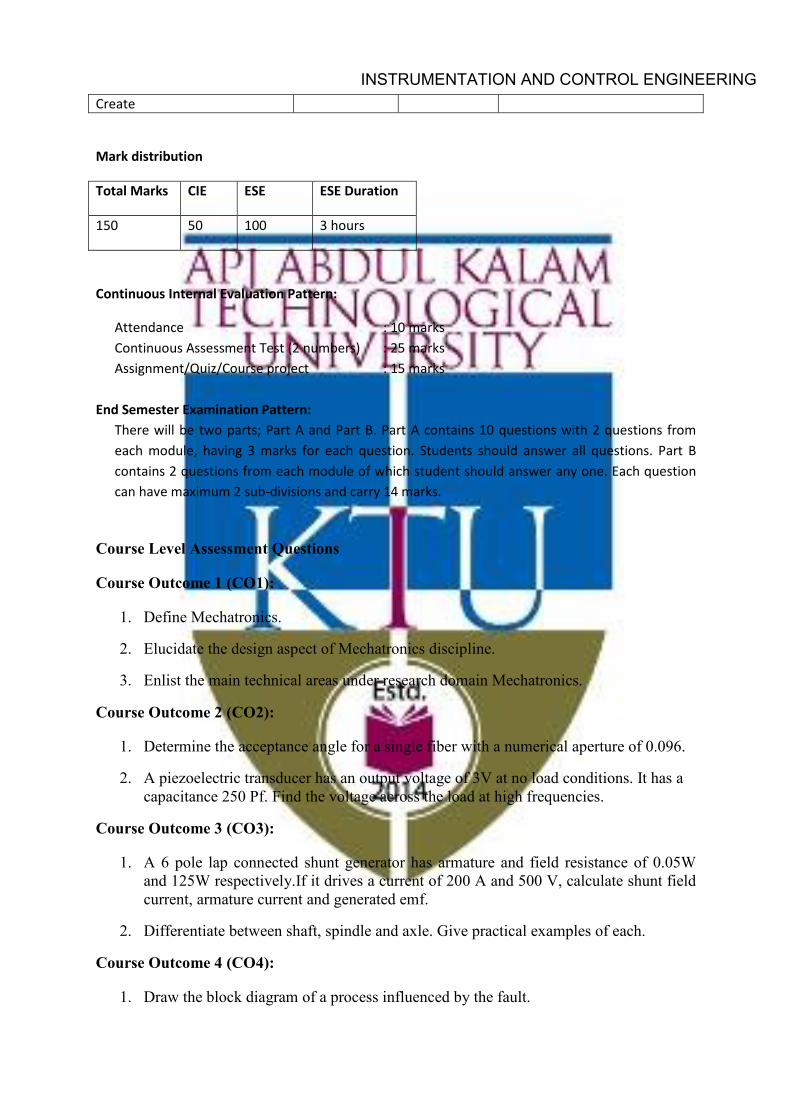
Create
Mark distribution
Total Marks CIE ESE ESE Duration
150 50 100 3 hours
Continuous Internal Evaluation Pattern:
Attendance : 10 marks Continuous Assessment Test (2 numbers) : 25 marks Assignment/Quiz/Course project : 15 marks
End Semester Examination Pattern:
There will be two parts; Part A and Part B. Part A contains 10 questions with 2 questions from each module, having 3 marks for each question. Students should answer all questions. Part B contains 2 questions from each module of which student should answer any one. Each question can have maximum 2 sub-divisions and carry 14 marks.
Course Level Assessment Questions
Course Outcome 1 (CO1):
1. Define Mechatronics.
2. Elucidate the design aspect of Mechatronics discipline.
3. Enlist the main technical areas under research domain Mechatronics.
Course Outcome 2 (CO2):
1. Determine the acceptance angle for a single fiber with a numerical aperture of 0.096.
2. A piezoelectric transducer has an output voltage of 3V at no load conditions. It has a capacitance 250 Pf. Find the voltage across the load at high frequencies.
Course Outcome 3 (CO3):
1. A 6 pole lap connected shunt generator has armature and field resistance of 0.05W and 125W respectively.If it drives a current of 200 A and 500 V, calculate shunt field current, armature current and generated emf.
2. Differentiate between shaft, spindle and axle. Give practical examples of each.
Course Outcome 4 (CO4):
1. Draw the block diagram of a process influenced by the fault.
INSTRUMENTATION AND CONTROL ENGINEERING
2. Discuss the various stages of the design process in terms of validation implementation.
Course Outcome 5 (CO5):
1. Why is the present trend towards flexible automation rather than fixed automation?
2. Give an overview of AGV architecture.
Model Question paper
Course Code: ICT294
Course Name:MECHATRONIC SYSTEMS
Max.Marks:100 Duration: 3 Hours
PARTA
Answer all Questions. Each question carries 3 Marks
1. Explain the purpose of standardization and importance of interchangeability. 2. Explain how electronic grade silicon can be produced. 3. A flat frequency response within10% is required from a piezoelectric crystal. Find the
value of minimum frequency for which it can be used if the time constant is 2ms.Find also the phase shift.
4. A diaphragm has a natural frequency of 30kHz.If both its diameter and thickness are halved, find the natural frequency.
5. A 220 V DC shunt motor takes 10 kW at a speed of 700 RPM. The armature resistance is 0.50 Ohm and the brush contact drop is 1.6 V mechanical and iron losses are 495 W. Calculate the efficiency and net torque.
6. Which type of bearing in nanotechnology conformant machineries. Why? 7. Give an illustration how the neural network concept has been adopted in the
engineering domain. 8. Why diagnosis is essential in Mechatronic system? Explain. 9. What do you mean by flexible manufacturing? What are the components of flexible
manufacturing? Explain. 10. Explain the role of electromagnetic balancer in HSSS.
PART B
Answer any onefull question from each module. Each question carries 14 Marks
Module 1
INSTRUMENTATION AND CONTROL ENGINEERING
11. (a) Mechatronics is the synergistic integration of mechanical engineering with electronics and intelligent control algorithms in the design and manufacture of products process. Justify the statement. (7) (b) How has Mechatronics discipline been evolved? Briefly explain various evolution stages. (7)
12. Explain the principle of operation of the following encoders. (i) What is lithography? Explain. (7) (ii) Discuss in detail on IC packaging. (7)
Module 2
13. (a) A Bimetal cantilever with invar, and brass as two metal strips of equal thickness has a total thickness of 0.125 cm and length 5 cm. Its one end is fixed, estimate the end deflection for the change of temperature of 40. (7) (b) A metallic diaphragm of thickness 3mm used for the measurement of a differential pressure 2kg/𝑐𝑐𝑐𝑐2 is required to give a deflection of its centre by 1 mm. What should be its diameter if the Young’s modulus and Poisson’s ratio of the element are 1, 00,000 kg/𝑐𝑐𝑐𝑐2 and 0.3 respectively. (7)
14. (a) A Hall Effect transducer is used for measurement of a magnetic field of 1.5 Wb/𝑐𝑐2with a copper transducer for which the Hall effect co-efficient is -5x10⁻¹²V-m/A-Wb/𝑐𝑐−2.The thickness of the element is 2mm and the current passing is 5A, find the voltage generated. (7) (b) A strain gauge has a resistance of 120Ω unstrained and the gauge factor is -12.What is the resistance value if the strain is 1%? (7)
Module 3
15. Two spur gears of 30 teeth and 40 teeth of 8mm module and 20° pressure angle are in mesh .Addendum of each gear is 7.5mm .The teeth are of involute form. Determine i) The angle through which the pinion turns while any pair of teeth are in
contact ii) The velocity of sliding between teeth when the contact on the pinion is at a radius of 101mm.The speed of the pinion is 445 rpm.
16. Define gear ratio. With a suitable example, illustrate how to calculate gear ratio.
Module 4
17. Draw the general architecture of a model based FDI scheme and explain.
18. Discuss in detail on artificial neural network.
Module 5
19. What is SEA scheme? Explain in detail.
20. Draw and explain a possible scheme for smart motorized actuator integration.
INSTRUMENTATION AND CONTROL ENGINEERING
Syllabus
MECHATRONIC SYSTEMS
Module 1 (8 Hours)
Introduction to Mechatronics
Introduction -multidisciplinary scenario – origins – evolution of Mechatronics – an overview of Mechatronics – brief introduction to manufacturing – design – Mechatronics in products-Scope of Mechatronics-advantages and disadvantages - applications.
Integrated circuit and printed circuit board manufacture
Integrated circuit fabrication-Production of electronic grade silicon-Growing a single crystal- Film deposition and oxidation. Printed circuit boards-Starting boards,-Board preparation- Circuit pattern imaging and etching-Hole drilling-Plating-Testing-Finishing-Assembly- Surface mounted devices.
Module 2 (9 Hours)
Transducers and Sensors
Difference between transducer and sensor – transducer types – transduction principle – photoelectric transducers – thermistors – thermo devices – thermocouple – inductive transducers – capacitive transducers – pyro electric transducers – piezoelectric transducer – hall-effect transducer – ionisation transducers – light emitting diode – optical encoder – bimetallic strip – bourdon tube – strain gauge – load cell diaphragms – mechanical switches – flow transducers – fibre optic transducers.
Module 3 (10 Hours)
Actuators and Mechanisms
Actuator types and application areas – electromechanical actuators – DC motor – AC motors – pneumatic actuators – Fluid power actuators – piezoelectric actuators – magneto strictive actuators – memory metal actuator – ion exchange polymer metal composites – chemical actuator – mechanisms – bearings – belt & chain – pulleys – gears – rack and pinion – ratchet, pawl & crank – slider and crank – cams and followers – Geneva wheel – four bar linkages.
Module 4 (8 Hours)
Feedback and Intelligent Control
INSTRUMENTATION AND CONTROL ENGINEERING
Defining automatic control methods – Artificial Neural Network-Fuzzy logic-Diagnostics: mathematical description of process and faults, FDI phases - FDI approaches- merits and demerits – analog versus digital control.
Components Based Modular Design and System Validation
Introduction-Components based modular design view – system validation – validation methodology – more about validation scheme – fusion technique.
Module 5 (10 Hours)
Integration
Background – advanced actuators – consumer mechatronic products – hydraulic fingers – surgical equipment – industrial robot – autonomous guided vehicle – drilling machine – conveyor based material handling systems
Mechatronic Design Strategy
spindle system review – dynamic modelling of HSSS – important design criteria – diagnostics and prognostics – sea scheme – approach to the design of a control systems – remote monitoring and control.
Text Books
1. Nitaigour Premchand Mahalik, “Mechatronics: Principles, Concepts and Applications”, McGraw Hill Education.
2. A.K Sawhney, “A course in Electrical and Electronic Measurements and Instrumentation”, Dhanpat Rai & Co. (P) Limited.
3. D. Patranabis, “Sensor & transducers”, Prentice Hall India Learning Private Limited, 2/e.
4. Godfrey Onwubolu “Mechatronics-Principles and Applications”,Butterworth-Heinemann.
Reference Books
1. M.D.Singh & J.G.Joshi, “Mechatronics”, Prentice Hall India Learning Private Limited.
2. Yoram Koren, “Computer Control of Manufacturing Systems”, McGraw Hill Education, 1/e.
INSTRUMENTATION AND CONTROL ENGINEERING
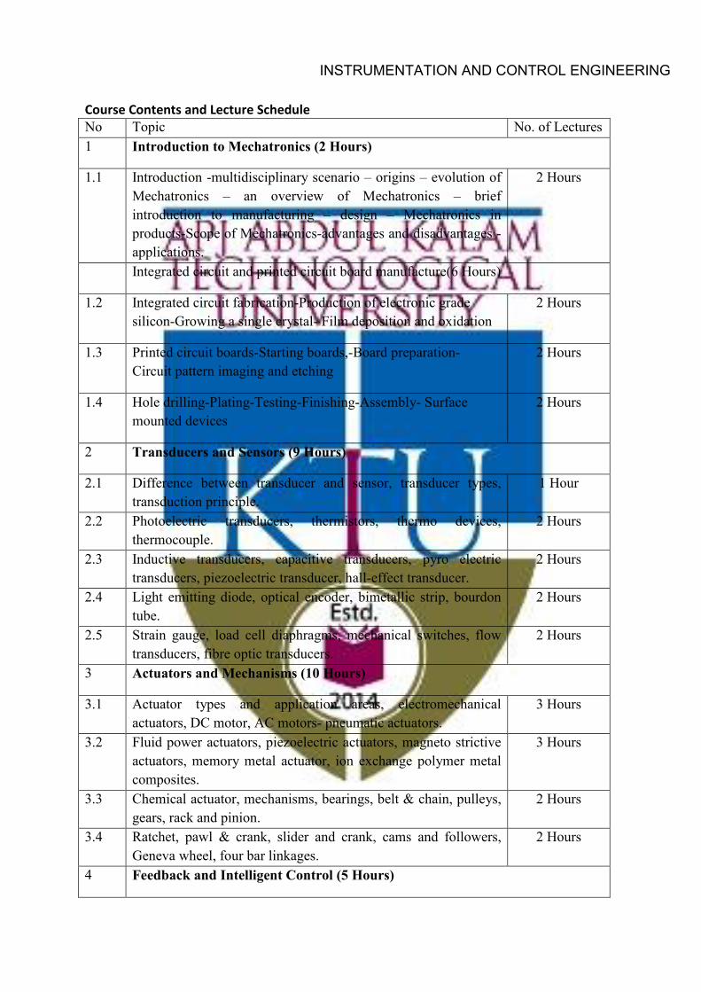
Course Contents and Lecture Schedule No Topic No. of Lectures 1 Introduction to Mechatronics (2 Hours)
1.1 Introduction -multidisciplinary scenario – origins – evolution of Mechatronics – an overview of Mechatronics – brief introduction to manufacturing – design – Mechatronics in products-Scope of Mechatronics-advantages and disadvantages - applications.
2 Hours
Integrated circuit and printed circuit board manufacture(6 Hours)
1.2 Integrated circuit fabrication-Production of electronic grade silicon-Growing a single crystal- Film deposition and oxidation
2 Hours
1.3 Printed circuit boards-Starting boards,-Board preparation- Circuit pattern imaging and etching
2 Hours
1.4 Hole drilling-Plating-Testing-Finishing-Assembly- Surface mounted devices
2 Hours
2 Transducers and Sensors (9 Hours)
2.1 Difference between transducer and sensor, transducer types, transduction principle.
1 Hour
2.2 Photoelectric transducers, thermistors, thermo devices, thermocouple.
2 Hours
2.3 Inductive transducers, capacitive transducers, pyro electric transducers, piezoelectric transducer, hall-effect transducer.
2 Hours
2.4 Light emitting diode, optical encoder, bimetallic strip, bourdon tube.
2 Hours
2.5 Strain gauge, load cell diaphragms, mechanical switches, flow transducers, fibre optic transducers.
2 Hours
3 Actuators and Mechanisms (10 Hours)
3.1 Actuator types and application areas, electromechanical actuators, DC motor, AC motors- pneumatic actuators.
3 Hours
3.2 Fluid power actuators, piezoelectric actuators, magneto strictive actuators, memory metal actuator, ion exchange polymer metal composites.
3 Hours
3.3 Chemical actuator, mechanisms, bearings, belt & chain, pulleys, gears, rack and pinion.
2 Hours
3.4 Ratchet, pawl & crank, slider and crank, cams and followers, Geneva wheel, four bar linkages.
2 Hours
4 Feedback and Intelligent Control (5 Hours)
INSTRUMENTATION AND CONTROL ENGINEERING
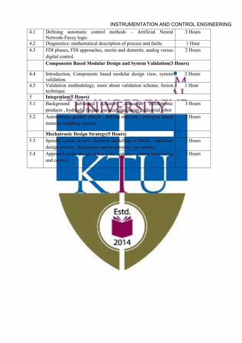
4.1 Defining automatic control methods – Artificial Neural Network-Fuzzy logic
3 Hours
4.2 Diagnostics: mathematical description of process and faults 1 Hour 4.3 FDI phases, FDI approaches, merits and demerits, analog versus
digital control. 2 Hours
Components Based Modular Design and System Validation(3 Hours)
4.4 Introduction, Components based modular design view, system validation.
2 Hours
4.5 Validation methodology, more about validation scheme, fusion technique.
1 Hour
5 Integration(5 Hours) 5.1 Background ,advanced actuators ,consumer mechatronic
products , hydraulic fingers ,surgical equipment ,industrial robot 3 Hours
5.2 Autonomous guided vehicle , drilling machine , conveyor based material handling systems
2 Hours
Mechatronic Design Strategy(5 Hours) 5.3 Spindle system review ,dynamic modelling of HSSS , important
design criteria , diagnostics and prognostics ,sea scheme 3 Hours
5.4 Approach to the design of a control systems – remote monitoring and control.
2 Hours
INSTRUMENTATION AND CONTROL ENGINEERING
Recommended