PACIFIC EARTHQUAKE ENGINEERING RESEARCH CENTER
Technical Manual for Strata
Albert R. KottkeEllen M. Rathje
University of Texas, Austin
PEER 2008/10february 2009

Technical Manual for Strata
Albert R. Kottke Department of Civil, Architectural, and Environmental Engineering
University of Texas, Austin
Ellen M. Rathje Department of Civil, Architectural, and Environmental Engineering
University of Texas, Austin
PEER Report 2008/10 Pacific Earthquake Engineering Research Center
College of Engineering University of California, Berkeley
February 2009

iii
ABSTRACT
The computer program Strata performs equivalent-linear site response analysis in the frequency
domain using time domain input motions or random vibration theory (RVT) methods, and allows
for randomization of the site properties. The following document explains the technical details of
the program, and provides a user's guide.
Strata is distributed under the GNU General Public License, which can be found at
http://www.gnu.org/licenses/.

iv
ACKNOWLEDGMENTS
This project was sponsored by the Pacific Earthquake Engineering Research Center’s Program of
Applied Earthquake Engineering Research of Lifelines Systems supported by the California
Department of Transportation and the Pacific Gas and Electric Company.
This work made use of the Earthquake Engineering Research Centers Shared Facilities
supported by the National Science Foundation under award number EEC-9701568 through the
Pacific Earthquake Engineering Research Center (PEER). Any opinions, findings, and
conclusions or recommendations expressed in this material are those of the authors and do not
necessarily reflect those of the funding agencies.
Additional support provided by the U.S. Nuclear Regulatory Commission is gratefully
acknowledged.

v
CONTENTS
ABSTRACT.................................................................................................................................. iii
ACKNOWLEDGMENTS ........................................................................................................... iv
TABLE OF CONTENTS ............................................................................................................. v
LIST OF FIGURES .................................................................................................................... vii
LIST OF TABLES ....................................................................................................................... xi
1 INTRODUCTION ................................................................................................................ 1
2 SITE RESPONSE ANALYSIS............................................................................................ 3
2.1 Equivalent-Linear Site Response Analysis .................................................................... 3
2.1.1 Linear Elastic Wave Propagation........................................................................3
2.1.2 Equivalent-Linear Analysis................................................................................ 8
2.1.3 Dynamic Soil Properties .................................................................................. 10
2.2 Site Response Methods ................................................................................................ 16
2.2.1 Time Series Method ......................................................................................... 16
2.2.2 Random Vibration Theory Method.................................................................. 19
3 VARIATION OF SITE PROPERTIES............................................................................ 29
3.1 Introduction...................................................................................................................29
3.2 Random Variables.........................................................................................................29
3.3 Statistical Models for Soil Properties............................................................................32
3.3.1 Layering and Velocity Model ...........................................................................32
3.3.2 Depth to Bedrock Model...................................................................................44
3.3.3 Nonlinear Soil Properties Model.......................................................................45
4 USING STRATA ................................................................................................................ 47
4.1 Strata Particulars ...........................................................................................................47
4.1.1 Auto-Discretization of Layers.......................................................................... 47
4.1.2 Interaction with Tables..................................................................................... 48
4.1.3 Nonlinear Curves ............................................................................................. 49
4.1.4 Recorded Motion Dialog Box .......................................................................... 52
4.1.5 Results Page ..................................................................................................... 53

vi
4.2 Glossary of Fields .........................................................................................................55
4.2.1 General Settings Page ...................................................................................... 56
4.2.2 Soil Types Page................................................................................................ 59
4.2.3 Soil Profile Page............................................................................................... 62
4.2.4 Motion(s) Page ................................................................................................. 65
4.2.5 Output Specification Page................................................................................ 70
4.3 Examples .......................................................................................................................72
4.3.1 Example 1: Basic Time Domain ...................................................................... 73
4.3.2 Example 2: Time Series with Multiple Input Motions .................................... 78
4.3.3 Example 3: RVT and Site Variation ................................................................ 79
REFERENCES............................................................................................................................ 83

vii
LIST OF FIGURES
Figure 2.1 Notation used in wave equation ..................................................................................4
Figure 2.2 Nomenclature for theoretical wave propagation .........................................................5
Figure 2.3 Representation of difference between outcrop and within motions. Outcrop
motions have upward and downward components that are equal, while within
motions have upward and downward motions that differ. ..........................................6
Figure 2.4 Input to surface transfer functions site in Table 2.1, considering different types of
input. ............................................................................................................................8
Figure 2.5 Example of strain time history and effective strain ( effγ ) ...........................................9
Figure 2.6 Example shear-wave velocity profile. .......................................................................12
Figure 2.7 Examples of shear modulus reduction and material damping curves for soil. ..........13
Figure 2.8 Nonlinear soil properties predicted by Darendeli (2001) model. ..............................15
Figure 2.9 Mean and mean σ± nonlinear soil properties predicted by Darendeli (2001). ........16
Figure 2.10 Time domain method sequence: (a) input acceleration time-series, (b) input
Fourier amplitude spectrum, (c) transfer function from input to surface, (d) surface
Fourier amplitude spectrum, and (e) surface acceleration time-series (after
Kramer 1996).............................................................................................................18
Figure 2.11 Comparison between target response spectrum and response spectrum computed
with RVT. ..................................................................................................................25
Figure 2.12 Relative error between computed response spectra and target response
spectrum. ...................................................................................................................25
Figure 2.13 FAS computing through inversion process. ..............................................................26
Figure 2.14 RVT method sequence: (a) input Fourier amplitude spectrum, (b) transfer
function from input to surface, and (c) surface Fourier amplitude spectrum. ...........28
Figure 3.1 Two variables with a correlation coefficient of: (a) 0.0, (b), 0.99, and (c) -0.7. .......31
Figure 3.2 Ten-layer profile modeled by a homogeneous Poisson process with λ = 1. .............34
Figure 3.3 Transforming from constant rate of λ = 1 to constant rate of λ = 0.2. ......................35
Figure 3.4 Ten-layer profile modeled by a homogeneous Poisson process with λ = 0.2. ..........35

viii
Figure 3.5 Toro (1995) layering model:. (a) occurrence rate (λ) as function of depth (d), and
(b) expected layer thickness (h) as function of depth................................................37
Figure 3.6 Transformation between homogeneous Poisson process with rate 1 to Toro
(1995) non-homogeneous Poisson process. ..............................................................38
Figure 3.7 Layering simulated with non-homogeneous Poisson process defined by
Toro (1995)................................................................................................................38
Figure 3.8 Ten generated shear-wave velocity (vs) profiles for USGS C site class: (a) using
generic layering and median vs, and (b) using user-defined layering and
median vs....................................................................................................................44
Figure 3.9 Generated nonlinear properties assuming perfect negative correlation. ...................46
Figure 4.1 Location selection (a) top of bedrock, (b) switching to fixed depth, and (c) fixed
depth specified as 15. ................................................................................................48
Figure 4.2 By clicking on button circled in red, all rows in table are selected...........................49
Figure 4.3 Nonlinear curve manager. .........................................................................................51
Figure 4.4 Initial view of Recorded Motion dialog box. ............................................................53
Figure 4.5 Example of completed Recorded Motion dialog box................................................53
Figure 4.6 Using Output view to examine results of calculation................................................55
Figure 4.7 Screenshot of Project group box................................................................................56
Figure 4.8 Screenshot of Type of Analysis group box. ..............................................................57
Figure 4.9 Screenshot of Site Property Variation group box......................................................57
Figure 4.10 Screenshot of Equivalent-Linear Parameters group box. ..........................................58
Figure 4.11 Screenshot of Layer Discretization group box. .........................................................58
Figure 4.12 Screenshot of Soil Types group box..........................................................................59
Figure 4.13 Screenshot of Bedrock Layer group box. ..................................................................59
Figure 4.14 Screenshot of Nonlinear Curve Variation Parameters group box. ............................60
Figure 4.15 Screenshot of Darendeli and Stokoe Model Parameters group box. .........................60
Figure 4.16 Screenshot of Nonlinear Property group box. ...........................................................61
Figure 4.17 Screenshot of Velocity Layers group box. ................................................................62
Figure 4.18 Screenshot of Velocity Variation Parameters group box. .........................................63
Figure 4.19 Screenshot of Layer Thickness Variation group box. ...............................................64
Figure 4.20 Screenshot of Bedrock Depth Variation group box. .................................................64

ix
Figure 4.21 Screenshot of Motion Input Location group box. .....................................................65
Figure 4.22 Screenshot of Recorded Motions table......................................................................65
Figure 4.23 Screenshot of Properties group box for RVT motion................................................66
Figure 4.24 Screenshot of Fourier Amplitude Spectrum group box.............................................67
Figure 4.25 Screenshot of Acceleration Response Spectrum group box......................................68
Figure 4.26 Screenshot of the Point Source Model group box used to define input RVT
motion using seismological source theory ................................................................69
Figure 4.27 Screenshot of Crustal Velocity Model group box. ....................................................70
Figure 4.28 Screenshot of Response Location Output group box. ...............................................70
Figure 4.29 Screenshot of Ratio Output group box. .....................................................................71
Figure 4.30 Shear-wave velocity profile of Sylmar County Hospital Parking Lot site (Chang
1996)..........................................................................................................................73
Figure 4.31 Example plot with multiple responses.......................................................................79
xi
LIST OF TABLES
Table 2.1 Site properties of example site..................................................................................... 6
Table 2.2 Values of RVT calculation for input motion. ............................................................ 26
Table 2.3 Values of RVT calculation for surface motion.......................................................... 27
Table 3.1 Categories of geotechnical subsurface conditions (third letter) in GeoMatrix site
classification Toro (1995).......................................................................................... 41
Table 3.2 Site categories based on Vs30 (Toro (1995)). ............................................................. 41
Table 3.3 Coefficients for Toro (1995) model........................................................................... 42
Table 3.4 Median shear-wave velocity (m/s) based on generic site classification. ................... 42
Table 4.1 Soil profile at Sylmar County Hospital Parking Lot site (Chang 1996). Mean
effective stress ( mσ ′ ) is computed assuming k0 of 1/2 and water table depth
of 46 m........................................................................................................................72
Table 4.2 Suite of input motions used in Example 2 ................................................................. 78

1 Introduction
The computer program Strata performs equivalent-linear site response analysis in the frequency
domain using time domain input motions or random vibration theory (RVT) methods, and allows
for randomization of the site properties. Strata was developed with financial support provided by
the Lifelines Program of the Pacific Earthquake Engineering Research (PEER) Center under
grant SA5405-15811 and funding from the Nuclear Regulatory Commission. Strata is distributed
under the GNU General Public License which can be found at http://www.gnu.org/licenses/.
The following document explains the technical details of the program. Chapter 2 provides
an introduction to equivalent-linear elastic wave propagation using both time series and random
vibration theory methods. Using the time series method, a single motion is propagated through
the site to compute the strain-compatible ground motion at the surface of the site or at any depth
in the soil column. Using random vibration theory, the expected maximum response is computed
from a mean Fourier amplitude spectrum (amplitude only), and duration. Chapter 3 introduces
random variables and the models that Strata uses to govern the variability of the site properties
(nonlinear properties, layering thickness, shear-wave velocity, and depth to bedrock). Chapter 4
introduces Strata's graphical user interface, along with several tutorials that introduce the
program's features.

3
2 Site Response Analysis
Strata computes the dynamic site response of a one-dimensional soil column using linear wave
propagation with strain-dependent dynamic soil properties. This is commonly referred to as the
equivalent-linear analysis method, which was first used in the computer program SHAKE
(Schnabel et al. 1972; Idriss and Sun 1992). Similar to SHAKE, Strata computes only the
response for vertically propagating, horizontally polarized shear waves propagated through a site
with horizontal layers.
The following chapter introduces strain-dependent soil properties, linear-elastic wave
propagation through a layered medium, and the equivalent-linear approach to site response
analysis.
2.1 EQUIVALENT-LINEAR SITE RESPONSE ANALYSIS
2.1.1 Linear Elastic Wave Propagation
For linear elastic, one-dimensional wave propagation, the soil is assumed to behave as a Kelvin-
Voigt solid, in which the dynamic response is described using a purely elastic spring and a
purely viscous dashpot (Kramer 1996). The solution to the one-dimensional wave equation for a
single wave frequency (ω) provides displacement (u) as a function of depth (z) and time (t)
(Kramer 1996):
( ) ( )exp expu(z,t) = A i t + k*z +B i t k*zω ω⎡ ⎤ ⎡ ⎤−⎣ ⎦ ⎣ ⎦ (2.1)
In Equation (1.1), A and B represent the amplitudes of the upward (-z) and downward
(+z) waves, respectively (Fig. 2.1). The complex wave number (k*) in Equation (2.1) is related to
the shear modulus (G), damping ratio (D), and mass density (ρ) of the soil using:

4
**= s
kvω (2.2)
**s
G v ρ= (2.3)
( ) ( )2 2* 1 2 2 1 1 2G G D i D D G i D= − + − ≅ + (2.4)
G* and vs* are called the complex shear modulus and complex shear-wave velocity,
respectively. If the damping ratio (D) is small (<10–20%), then the approximation of the
complex shear modulus in Equation (2.4) is appropriate. Strata uses the complete definition of
the complex shear modulus, not the approximation, in the calculations.
Fig. 2.1 Notation used in wave equation.
Equation (2.1) applies only to a single layer with uniform soil properties, and the wave
amplitudes (A and B) can be computed from the layer boundary conditions. For a layered system,
shown in Figure 2.1, the wave amplitudes are calculated using recursive formulas developed by
maintaining compatibility of displacement and shear stress at the layer boundaries. Using these
assumptions, the following recursive formulas are developed (Kramer 1996):
( ) ( )
( ) ( )*
**1
*1
1
21 exp 1 exp
1 exp 1 exp
12 2 2
1 12 2 2 2m
* *m m m m
m m m m m
* *m m m m
mm+ mm
ik h ik h BaA A
ik h ik hB BA a
a
a
+⎛ ⎞ ⎛ ⎞
= + + − −⎜ ⎟ ⎜ ⎟⎝ ⎠ ⎝ ⎠⎛ ⎞ ⎛ ⎞
= − + + −⎜ ⎟ ⎜ ⎟⎝ ⎠ ⎝ ⎠
(2.5)

5
where m is the layer number, hm is the layer height and αm* is the complex impedance ratio. The complex impedance ratio is defined as:
**,
* *1 1 1 , 1
*m s m* m m
mm m m s m
vk Ga = k G v
ρρ+ + + +
= (2.6)
At the surface of the soil column (m=1), the shear stress must equal zero and the
amplitudes of the upward and downward waves must be equal (A1=B1).
Fig. 2.2 Nomenclature for theoretical wave propagation.
The wave amplitudes (A and B) within the soil profile are calculated at each frequency
(assuming known stiffness and damping within each layer) and are used to compute the response
at the surface of a site. This calculation is performed by setting A1=B1=1.0 at the surface and
recursively calculating the wave amplitudes (Am+1,Bm+1) in successive layers until the input
(base) layer is reached. The transfer function between the motion in the layer of interest (m) and
in the rock layer (n) at the base of the deposit is defined as:
( )
( )( )
( ) m m mm,n
n n n
u A + BTF = = u A + B
ωω
ω (2.7)
where ω is the frequency of the harmonic wave. The transfer function is the ratio of the
amplitude of harmonic motion—either displacement, velocity, or acceleration—between two
layers of interest and varies with frequency. The transfer function (surface motion/within

6
motion) for the site with the properties presented in Table 2.1 is shown in Figure 2.3. The
locations of the peaks in the transfer function are controlled by the modes of vibration of the soil
deposit. The peak at the lowest frequency represents the fundamental (i.e., first) mode of
vibration and results in the largest amplification. The peaks at higher frequencies are the higher
vibrational modes of the site.
For the example site (Table 2.1), the first mode natural frequency is 1.75 Hz (site period
= 0.57 s). In the transfer function (Fig. 2.3), the peak with the largest amplification occurs at this
frequency. The amplitudes of the peaks are controlled by the damping ratio of the soil. As the
damping of the system increases, the amplitudes of the peaks decrease, which results in less
amplification.
Table 2.1 Site properties of example site.
Property Rock Soil Mass Density (ρ) 2.24 g/cm3 1.93 g/cm3 Height (h) Inf 50 m Shear-wave Velocity (vs) 1500 m/s 350 m/s Damping ratio (D) 1% 7%
Fig. 2.3 Representation of difference between outcrop and within motions. Outcrop motions have upward and downward components that are equal, while within motions have upward and downward motions that differ.

7
The response at the layer of interest is computed by multiplying the Fourier amplitude
spectrum of the input rock motion by the transfer function:
( ) ( ) ( )m m,n nY = TF Yω ω ω (2.8)
where Yn is the input Fourier amplitude spectrum at layer n, and Ym is the Fourier amplitude
spectrum at the top of the layer of interest. The Fourier amplitude spectrum of the input motion
can be defined using a variety of methods and is discussed further in Sections 2.2.1 and 2.2.2.
One issue that must be considered is that the input Fourier spectrum typically represents a
motion recorded on rock at a free surface (i.e., the ground surface), where the upgoing and
downgoing wave amplitudes are equal (A1 + B1), rather than on rock at the base of a soil deposit,
where the wave amplitudes are not equal (Fig. 2.4). The change in boundary conditions (An = Bn
for a free surface, An ≠ Bn at the base of a soil deposit) must be taken into account. The motions
at any free surface are referred to as outcrop motions and their amplitudes are described by twice
the amplitude of the upward wave (2A). A transfer function can be defined that converts an
outcrop motion into a within motion, and this transfer function can be combined with the transfer
function in Equation (2.3) to create a transfer function that can be applied to recorded outcrop
motions on rock (Eq. 2.9).
( ), 2n n m m
m nn n n
outcrop within to layerto within n
A + B A + BTF =
A A + Bω •
(2.9)
Motions recorded at depth (e.g., recorded in a borehole) are referred to as within motions
and for these motions the transfer function given in Equation (2.7) can be used. Figure 2.3 shows
the transfer function (surface motion/outcrop motion) for the site profile presented in Table 2.1
using Equation (2.9) where the input motion is specified as outcrop. In comparison with the
surface/within transfer function, the surface/outcrop transfer function displays less amplification
for all modes.

8
Fig. 2.4 Input to surface transfer functions site in Table 2.1 considering different types of input.
2.1.2 Equivalent-Linear Analysis
The previous section assumed that the soil was linear-elastic. However, soil is nonlinear, such
that the dynamic properties of soil (shear modulus, G, and damping ratio, D) vary with shear
strain, and thus the intensity of shaking. In equivalent-linear site response analysis, the nonlinear
response of the soil is approximated by modifying the linear elastic properties of the soil based
on the induced strain level. Because the induced strains depend on the soil properties, the strain-
compatible shear modulus and damping ratio values are iteratively calculated based on the
computed strain.
A transfer function is used to compute the shear strain in the layer based on the
outcropping input motion. In the calculation of the strain transfer function, the shear strain is
computed at the middle of the layer (z=hm/2) and used to select the strain-compatible soil
properties. Unlike the previous transfer functions that merely amplified the Fourier amplitude
spectrum, the strain transfer function amplifies the motion and converts acceleration into strain.
The strain transfer function based on an outcropping input motion is defined by:
9
( )( )
( )
,
* **
,2
exp exp2 2
2
m
strainm,n
n outcrop
m m m mm m m
2n
hz = TF =
u
ik h ik hik A B =
A
γ ωω
ω
ω
⎛ ⎞⎜ ⎟⎝ ⎠
⎛ ⎞⎛ ⎞ ⎛ ⎞− −⎜ ⎟⎜ ⎟ ⎜ ⎟⎜ ⎟⎝ ⎠ ⎝ ⎠⎝ ⎠
−
ii
(2.10)
The strain Fourier amplitude spectrum within a layer is calculated by applying the strain
transfer function to the Fourier amplitude spectrum of the input motion. The maximum strain
within the layer is derived from this Fourier amplitude spectrum—either through conversion to
the time domain or through RVT methods, further discussed in Section 2.2. However, it is not
appropriate to use the maximum strain within the layer to compute the strain-compatible soil
properties because the maximum strain occurs only for an instant. Instead, an effective strain
(γeff) is calculated from the maximum strain. Typically, the effective strain is 65% of the
maximum strain. An example of a strain time-series and the effective strain is shown in Figure
2.5.
Fig. 2.5 Example of strain time history and effective strain (γeff).

10
Equivalent-linear site response analysis requires that the strain-dependent nonlinear
properties (i.e., G and D) be defined. The initial (small strain) shear modulus (Gmax) is calculated
by:
2max sG vρ=
(2.11)
where ρ is the mass density of the site, and vs is the measured shear-wave velocity.
Characterizing the nonlinear behavior of G and D is achieved through modulus reduction and
damping curves that describe the variation of G/Gmax and D with shear strain (discussed in the
next section). Using the initial dynamic properties of the soil, equivalent-linear site response
analysis involves the following steps:
1. The wave amplitudes (A and B) are computed for each of the layers.
2. The strain transfer function is calculated for each of the layers.
3. The maximum strain within each layer is computed by applying the strain transfer
function to the input Fourier amplitude spectrum and finding the maximum response (see
Section 2.2).
4. The effective strain (γeff) is calculated from the maximum strain within each layer.
5. The strain-compatible shear modulus and damping ratio are recalculated based on the
new estimate of the effective strain within each layer.
6. The new nonlinear properties (G and D) are compared to the previous iteration and an
error is calculated. If the error for all layers is below a defined threshold the calculation
stops.
After the iterative portion of the program finishes, the dynamic response of the soil deposit is
computed using the strain-compatible properties.
2.1.3 Dynamic Soil Properties
In a dynamic system, the properties that govern the response are the mass, stiffness, and
damping. In soil under seismic shear loading, the mass of the system is characterized by the mass
density (ρ) and the layer height (h), the stiffness is characterized by the shear modulus (G), and
the damping is characterized by the viscous damping ratio (D). The dynamic behavior of soil is
challenging to model because it is nonlinear, such that both the stiffness and damping of the

11
system change with shear strain. Section 2.1.2 introduced equivalent-linear site response analysis
in which the nonlinear response of the soil was simplified into a linear system that used strain-
compatible dynamic properties (G and D). The analysis requires that the strain dependence of the
nonlinear properties within a layer be fully characterized.
Defining the mass density of the system is a straightforward process because the density
of soil falls within a limited range for soil, and a good estimate of the mass density can be made
based on soil type. Characterization of the stiffness and damping properties of soil is more
complicated, the most rigorous approach requiring testing in both the field and laboratory.
The shear modulus and material damping of the soil are characterized using the small
strain shear modulus (Gmax), modulus reduction curves that relate G/ Gmax to shear strain, and
damping ratio curves that relate D to shear strain. The small strain shear modulus is best
characterized by in situ measurement of the shear-wave velocity as a function of depth. An
example shear-wave velocity profile is shown in Figure 2.6. The profile tends to be separated
into discrete layers with a generally increasing shear-wave velocity with increasing depth.
Examples of modulus reduction and damping curves for soil are shown in Figure 2.7. These
curves show a decrease in the soil stiffness and an increase in the damping ratio with an increase
in shear strain.

12
Fig. 2.6 Example shear-wave velocity profile.
Modulus reduction and damping curves may be obtained from laboratory measurements
on soil samples or derived from empirical models based on soil type and other variables. One of
the most comprehensive empirical models was developed by Darendeli (2001) and is included
with Strata. The model expands on the hyperbolic model presented by Hardin and Drnevich
(1972) and accounts for the effects of confining pressure ( 0σ ′ ), plasticity index (PI),
overconsolidation ratio (OCR), frequency (f), and number of cycles of loading (N) on the
modulus reduction and damping curves.

13
Fig. 2.7 Examples of shear modulus reduction and material damping curves for soil.
In the Darendeli (2001) model, the shear modulus reduction curve is a hyperbola defined
by:
max
1 =
1a
r
GG γ
γ⎛ ⎞
+ ⎜ ⎟⎝ ⎠
(2.12)
where a is 0.9190, γ is the shear strain, and γref is the reference shear strain. The reference shear
strain (not in percent) is computed from:
( )
0.34830.3246 = 0.0352 + 0.0010 o
ra
PI OCRpσγ
′⎛ ⎞⎜ ⎟⎝ ⎠
(2.13)
where 0σ ′ is the mean effective stress and pa is the atmospheric pressure in the same units as 0σ ′ .
In the model, the damping ratio is calculated from the minimum damping ratio at small strains
(Dmin) and from the damping ratio associated with hysteretic Masing behavior (DMasing). The
minimum damping is calculated from:
( ) ( ) ( )( )0.2889 0.1069% 0.8005 0.0129 1 0.2919 1n min 0D = PI OCR fσ−′ −+ + (2.14)
where f is the excitation frequency (Hz). The computation of the Masing damping requires the
calculation of the area within the stress-strain curve predicted by the shear modulus reduction
curve. The integration can be approximated by:

14
( ) 2 3Masing 1 Masing, a=1 2 Masing, a=1 3 Masing, a=1D % = c D + c D + c D (2.15)
where:
( )Masing, a=1 2
1n100% 4 2
rr
r
r
+
D =
+
γ γγ γγ
γπγ γ
⎧ ⎫⎡ ⎤⎛ ⎞−⎪ ⎪⎢ ⎥⎜ ⎟
⎪ ⎪⎝ ⎠⎢ ⎥ −⎨ ⎬⎢ ⎥⎪ ⎪⎢ ⎥⎪ ⎪⎢ ⎥⎣ ⎦⎩ ⎭
(2.16)
21c = 1.1143a + 1.8618a + 0.2533−
22
23
c 0.0805a 0.0710a 0.0095c 0.0005a + 0.0002a + 0.0003
= − −
= − (2.17)
The minimum damping ratio in Equation (2.14) and the Masing damping in Equation
(2.16) are combined to compute the total damping ratio (D) using:
0.1
sinMa g minmax
GD = b D + DG
⎛ ⎞⎜ ⎟⎝ ⎠
(2.18)
where b is defined as:
= 0.6329 0.00571nb N− (2.19)
where N is the number of cycles of loading. In most site response applications, the number of
cycles (N) and the excitation frequency (f) in the model are defined as 10 and 1, respectively.
Figure 2.8 shows the predicted nonlinear curves for a sand (PI=0, OCR=1) at an effective
confining pressure of 1 atm.

15
Fig. 2.8 Nonlinear soil properties predicted by Darendeli (2001) model.
A Bayesian approach was used in the Darendeli (2001) model to calculate the model
coefficients. One of the unique aspects of this model is that the scatter of the data about the mean
estimate is quantified. In the Darendeli (2001) model, the variability about the mean value is
assumed to be normally distributed. The normal distribution is described using a mean and
standard deviation. The mean values are calculated from Equations (2.12) and (2.18). The
standard deviation is a function of the amplitude of the nonlinear property (i.e., G/Gmax and D).
The standard deviation of the normalized shear modulus (σNG) is computed by:
( ) ( )
( )
2
max
2max
0.25 = exp 4.23 +
exp 3.62 exp(3.62)
0.015 + 0.16 0.25 / 0.5
NG
GG
G G
σ
⎛ ⎞− 0.5⎜ ⎟
⎝ ⎠− −
= − −i
(2.20)
This model results in small σNG when G/Gmax is close to 1 or 0 and relatively large σNG
when G/Gmax is equal to 0.5. The standard deviation of the damping ratio (σD) is computed by:
( ) ( ) ( )( )
= exp 5.0 + exp 0.25 %
= 0.0067 + 0.78 %
D D
D
σ − −
i (2.21)
16
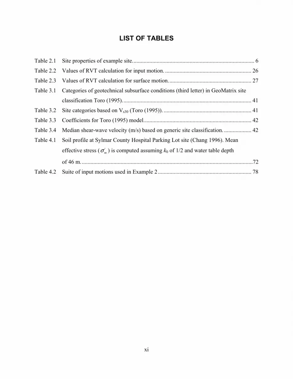
In the damping ratio model, σD increases with increasing damping ratio. Using these
definitions for the standard deviation, the +σ modulus reduction and damping curve for sand at a
confining pressure of 1 atm are shown in Figure 2.9.
Fig. 2.9 Mean and mean nonlinear soil properties predicted by Darendeli (2001).
2.2 SITE RESPONSE METHODS
The previous section introduced transfer functions that transform the input Fourier amplitude
spectrum (FAS) into a FAS of strain or acceleration; transfer functions can also be derived to
compute the response of a single-degree-of-freedom oscillator. In both the time domain and
random vibration theory methods, the same transfer functions are applied to the input FAS. The
difference in the methods is in how this FAS in the frequency domain is converted into time
domain information.
2.2.1 Time Series Method
In the time series method, an input acceleration time history is provided and the input FAS is
computed from that time series using the fast-Fourier transform (FFT) to compute the discrete
Fourier transformation on the provided time series. The computed FAS is complex valued, and
can be converted into amplitude and phase information. Strata uses the free and open-source
17
FFTW library (http://www.fftw.org). The inverse discrete Fourier transform is used to compute a
time series for a given FAS. The details of the FFT process are not discussed here, but can be
found on the FFTW webpage.
In Strata, the time series is padded with zeros to obtain a number of points that is a power
of two. If a time series contains a power of two values, then it is padded with zeros until the next
power of two.
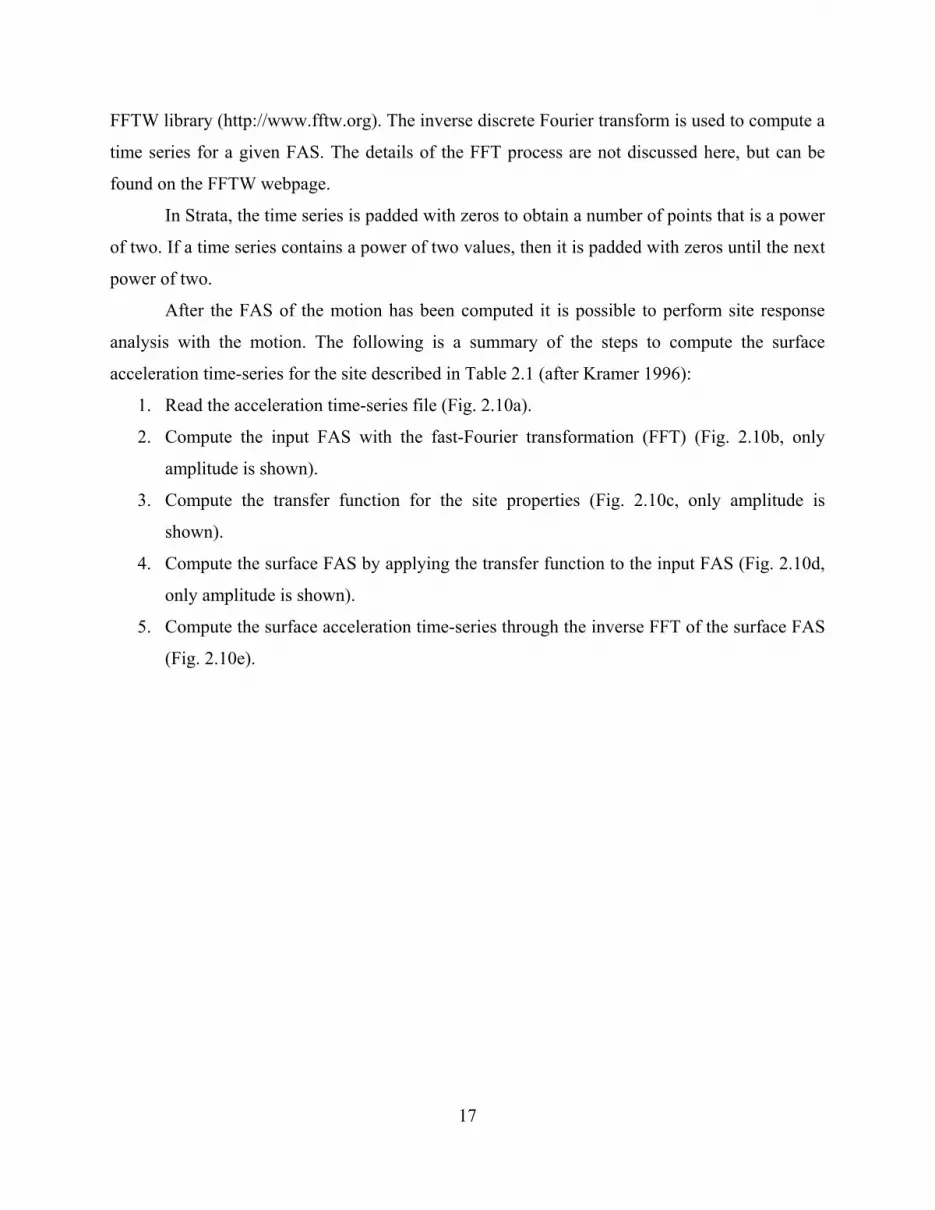
After the FAS of the motion has been computed it is possible to perform site response
analysis with the motion. The following is a summary of the steps to compute the surface
acceleration time-series for the site described in Table 2.1 (after Kramer 1996):
1. Read the acceleration time-series file (Fig. 2.10a).
2. Compute the input FAS with the fast-Fourier transformation (FFT) (Fig. 2.10b, only
amplitude is shown).
3. Compute the transfer function for the site properties (Fig. 2.10c, only amplitude is
shown).
4. Compute the surface FAS by applying the transfer function to the input FAS (Fig. 2.10d,
only amplitude is shown).
5. Compute the surface acceleration time-series through the inverse FFT of the surface FAS
(Fig. 2.10e).

18
Fig. 2.10 Time domain method sequence: (a) input acceleration time-series, (b) input Fourier amplitude spectrum, (c) transfer function from input to surface, (d) surface Fourier amplitude spectrum, and (e) surface acceleration time-series (after Kramer 1996).

19
2.2.2 Random Vibration Theory Method
The random vibration theory (RVT) approach to site response analysis was first proposed in the
engineering seismology literature (e.g., Schneider et al. (1991)) and has been applied to site
response analysis (Silva et al. 1997, Rathje and Ozbey 2006, Rathje and Kottke 2008). RVT does
not utilize time domain input motions, but rather initiates all computations with the input FAS
(amplitude only, no phase information). Because RVT does not have the accompanying phase
angles to the Fourier amplitudes, a time history of motion cannot be computed. Instead, extreme
value statistics are used to compute peak time domain parameters of motion (e.g., peak ground
acceleration, spectral acceleration) from the Fourier amplitude information. Due to RVT's
stochastic nature, one analysis can provide a median estimate of the site response with a single
analysis and without the need for time domain input motions.
2.2.2.1 RVT Basics
Random vibration theory can be separated into two parts: (1) conversion between time and
frequency domain using Parseval's theorem and (2) estimation of the peak factor using extreme
value statistics. Consider a time-varying signal x(t) with its associated Fourier amplitude
spectrum, X(f). The root-mean-squared value of the signal (xrms) is a measure of its average value
over a given time period, Trms, and is computed from the integral of the times series over that
time period:
( ) 2
0
1 = rmsT
rmsrms
x x t dtT
⎡ ⎤⎣ ⎦∫ (2.22)
Parseval's theorem relates the integral of the time series to the integral of its Fourier
transform such that Equation (2.22) can be written in term of the FAS of the signal:
( ) 2 0
0
2 = = rmsrms rms
mx x f dfT T
∞
∫ (2.23)
where m0 is defined as the zero-th moment of the FAS. The N-th moment of the FAS is defined
as:

20
( ) ( ) 2
0 2 2
n
nm f X f dfπ∞
= ∫ (2.24)
The peak factor (PF) represents the ratio of the maximum value of the signal (xmax) to its
rms value (xrms), such that if xrms and the PF are known, then xmax can be computed using:
max rmsx = PF xi
(2.25)
Cartwright and Longuet-Higgins (1956) studied the statistics of ocean wave amplitudes,
and considered the probability distribution of the maxima of a signal to develop expressions for
the PF in terms of the characteristics of the signal. Cartwright and Longuet-Higgins (1956)
derived an integral expression for the expected values of the peak factor in terms of the number
of extrema (Ne) and the bandwidth (ξ) of the time series (Boore 2003):
[ ] 2
0 = 2 1
eNzE PF e dzξ
∞ −⎡ ⎤−⎣ ⎦∫ (2.26)
where the bandwidth is defined as:
22
0 4
= mm m
ξ (2.27)
and the number of extrema are defined as:
4
2
= gme
T mNmπ
(2.28)
Boore (2003) illustrated the need to modify the duration used in the rms calculation when
considering requires modification for spectral acceleration to account for the enhanced duration
due to the oscillator response. Generally, adding the oscillator duration to the ground motion
duration will suffice, except in cases where the ground motion duration is short (Boore and
Joyner 1984). Boore and Joyner (1984) recommend the following expressions to define Trms:
0 = +
+
n
rms gm nT T T γγ α
⎛ ⎞⎜ ⎟⎝ ⎠
(2.29)
= gm
n
TT
γ
(2.30)

21
0 2
nTTπβ
= (2.31)
where T0 is the oscillator duration, Tn is the oscillator natural period, and β is the damping ratio
of the oscillator. Based on numerical simulations, Boore and Joyner (1984) proposed n=3 and
α=1/3 for the coefficients in Equation (2.29).
2.2.2.2 Defining Input Motion
The input motion in an RVT analysis is defined by a Fourier amplitude spectrum (FAS) and
ground motion duration (Tgm). The FAS can be directly computed using seismological source
theory (e.g., (Brune 1970, 1971)), or it can be back-calculated from an acceleration response
spectrum (see Section 2.2.4). When the FAS is directly provided, the frequencies provided with
the Fourier amplitude spectrum represent the frequency range used by the program, so it is
critical that enough points be provided.
Calculation of the duration for use in RVT analysis can be done using seismological
theory or empirical models. Boore (2003) recommends the following description of ground
motion duration (Tgm) for the western United States using seismological theory:
0
,
1= + 0.05R
p
s
gmPathduration, TSource
duration T
Tf
(2.32)
where R is the distance in km, and the corner frequency (f0) in hertz is given by:
13
60
0
= 4.9 10 sfM
σβ⎛ ⎞Δ⎜ ⎟⎝ ⎠
i (2.33)
where Δσ is the stress drop in bar, βs is the shear-wave velocity in units of km/s, and M0 is the
seismic moment in units of dyne-cm (Brune 1970). The seismic moment (M0) is related to the
moment magnitude (Mw) by:
( )+ 10.7
32
0 10 wMM = (2.34)
For the eastern United States, Campbell (1997) proposes that the path duration effect be
distance dependent:

22
0, 100.16 10 700.03 70 130
0.04 130p
R kmR, km < R km
T = R, km < R kmR, R> km
≤⎧⎪ ≤⎪⎪− ≤⎨⎪⎪⎪⎩
(2.35)
Empirical ground motion duration models such as Abrahamson and Silva (1996) can also
be used to estimate the duration of the scenario event (Tgm). When such a model is applied, it is
recommended that Tgm be taken as time between the buildup from 5% to 75% of the normalized
Arias intensity (D5-75).
2.2.2.3 Source Theory Model
Strata provides functionality for the calculation of a single-corner frequency ω2 point source
model originally proposed by Brune (1970) and more recently discussed in Boore (2003). The
default values for the western United States and the central and eastern United States are taken
from Campbell (1997).
2.2.2.4 Calculation of FAS from Acceleration Response Spectrum
The input rock FAS (Y(f)) can be derived from an acceleration response spectrum using an
inverse technique. The inversion technique follows the basic methodology proposed by
Gasparini and Vanmarcke (1976) and further described by Rathje et al. (2005). The inversion
technique makes use of the properties of the single-degree-of-freedom (SDOF) transfer function
used to compute the response spectral values. The square of the Fourier amplitude at the SDOF
oscillator natural frequency fn (|Y(fn)|2) can be written in terms of the spectral acceleration at fn
(na,fS ), the peak factor (PF), the rms duration of the motion (Trms), the square of the Fourier
amplitudes (|Y(f)|2) at frequencies less than the natural frequency, and the integral of the SDOF
transfer function (|Hfn(f)|2:

23
( )
( )( )
2,2 2
2 02
0
1 2
n
fna fnrmsn
f n
STY f Y f dfPFH f df f
∞
⎛ ⎞≅ −⎜ ⎟⎜ ⎟− ⎝ ⎠
∫∫
(2.36)
Within Equation (2.36), the integral of the transfer function is constant for a given natural
frequency and damping ratio (β), allowing the equation to be simplified to (Gasparini and
Vanmarcke 1976):
( ) ( )
2,2 2
2
1 21
4
nfa fnrmsn 0
n
STY f Y f dfPFf π
β
⎛ ⎞≅ −⎜ ⎟⎜ ⎟⎛ ⎞ ⎝ ⎠−⎜ ⎟
⎝ ⎠
∫ (2.37)
The peak factors in Equation (2.37) depend on the moments of the FAS, which is
currently undefined. So the peak factors for all natural frequencies are initially assumed to be
2.5.
Equation (2.37) is applied first to the spectral acceleration of the lowest frequency
(longest period) provided by the user. At this frequency, the FAS integral term in Equation (2.37)
can be assumed to be equal to zero. The equation is then applied at successively higher
frequencies using the previously computed values of |Y(fn)| to assess the integral.
To improve the agreement between the RVT-derived response spectrum ( ( )RVTaS f ) and
the target response spectrum ( Target ( )aS f ), the RVT-derived FAS is corrected by multiplying it by
the ratio of the two response spectra. This iterative process corrects the FAS from iteration i
(|Yi(f)|) using:
( ) ( ) ( )
( ) ( )1 Target= RVTa
i ia
S fY f Y f
S f+ i (2.38)
Additionally, the newly defined FAS is used to compute appropriate peak factors for each
frequency. The full procedure used to generate a corrected FAS is:
1. Initial FAS is computed using the Gasparini and Vanmarcke (1976) technique (Eq. 2.37).
2. The acceleration response spectrum associated with this FAS is computed using RVT.
3. The FAS is corrected using Equation (2.38).
4. The peak factors are updated.
5. Using the corrected FAS and new peak factors, a new acceleration response spectrum is
calculated.

24
This process is repeated until one of three conditions is met:
1. maximum of 30 iterations,
2. a root-mean-square-error of 0.005 is achieved between the RVT response spectrum and
the target response spectrum, or
3. change in the root-mean-square error is less than 0.001.
This ratio correction works very well in producing a FAS that agrees with the target
response spectrum, but the resulting FAS may have an inappropriate shape at some frequencies,
as discussed below.
To demonstrate the inversion process, consider a scenario event of magnitude 7 at a
distance of 20 km. The target response spectrum is computed using the Abrahamson and Silva
(1997) attenuation model (Fig. 2.11). An initial estimate of the FAS is computed using the
Gasparini and Vanmarcke (1976) method and then the ratio correction algorithm is applied. This
methodology (called Ratio Corrected) results in good agreement with the target response
spectrum (Fig. 2.11), with less than 5% relative error as shown in Figure 2.12. However, the
associated FAS slopes up at low and high frequencies (Fig. 2.13). The sloping up at low
frequencies can be mitigated by extending the frequency domain because the spectral
acceleration at a given frequency is affected by a range of frequencies in the FAS.
The frequency domain extension involves expanding frequencies to half of the minimum
frequency and twice the maximum frequency specified in the target response spectrum. For
example, if the target response spectrum is provided from 0.2 to 100 Hz (5 to 0.01 sec), then the
frequencies of the FAS are defined at points equally spaced in log space from 0.1 to 200 Hz. The
resulting response spectrum essentially displays the same agreement with the target response
spectrum (curve labeled Ratio and Extrapolated in Figs. 2.11 and 2.12), but the FAS shows no
sloping up at low frequencies and less sloping up at high frequencies (Fig. 2.13).
While the results in Figures 2.11–2.13 would appear to be adequate, it was observed that
the sloping up at high frequencies was affecting the RVT calculation. The peak factor depends
on the 4th moment of the FAS (Eqs. 2.27–2.28), which is more sensitive to higher frequencies.
Additionally, seismological theory indicates that the slope of the FAS at high frequencies should
be increasingly negative due to a path-independent loss of the high-frequency motion (Boore
2003). To deal with these issues, the slope of the FAS at high frequencies is forced down (curve
labeled Ratio, Extrap., & Slope Forced in Fig. 2.13). The corrected portion of the FAS is

25
computed through linear extrapolation in log-log space from where the slope deviates from its
steepest value by more than 5%. This solution results in a slight under prediction (~3%) of the
peak ground acceleration (Figs. 2.11 and 2.12).
Fig. 2.11 Comparison between target response spectrum and response spectrum computed with RVT.
Fig. 2.12 Relative error between computed response spectra and target response spectrum.

26
Fig. 2.13 FAS computing through inversion process.
2.2.2.5 Example of RVT Procedure
The following is an example of random vibration theory applied to site response analysis to
estimate the peak acceleration at the top of the site described in Table 2.1. The earthquake
scenario is a magnitude 7 event at a distance of 20 km, as described in the previous section.
1. Empirical relationships are used to specify the input rock response spectrum (Fig. 2.11)
and ground motion duration (Tgm = D5-75 = 8.2 s).
2. Using the inversion technique, the FAS corresponding to the target response spectrum is
computed (Fig. 2.14a). In this example, the peak acceleration of the input motion is
computed with RVT to allow for a comparison in the peak response between the surface
and the input. The RVT calculation results are shown in Table 2.2.
Table 2.2 Values of RVT calculation for input motion.
Parameter Value EquationMoments of FAS (m0, m2, m4) 0.0280, 93.84, 1.738x10⁷ 2.28
Bandwidth 0.1346 2.31 Number of extrema (Ne) 1123 2.32 Peak factor (PF) 3.325 2.30 Root-mean-square acceleration (arms) 0.0584 g 2.27 Expected peak acceleration from RVT (amax) 0.1942g 2.29 Target peak acceleration (PGA) 0.20 g ---

27
3. Compute the transfer function for the site properties (Fig. 2.14b).
4. Compute the surface FAS by applying the absolute value of the transfer function to the
input FAS (Fig. 2.14c). Using the surface FAS, the expected peak acceleration can be
computed using RVT, as presented in Table 2.3. The calculation shows that the site
response increases the peak ground acceleration by approximately 38%.
Table 2.3 Values of RVT calculation for surface motion.
Parameter Value EquationMoments of FAS (m0, m2, m4) 0.0635, 39.6356, and
1.6306x10⁷ 2.28
Bandwidth 0.3895 2.31 Number of extrema (Ne) 167.414 2.32 Peak factor (PF) 3.0588 2.30 Root-mean-square acceleration (arms) 0.0880 g 2.27 Expected maximum acceleration (amax) 0.2692 g 2.29 Target peak acceleration (PGA) 0.20 g ---
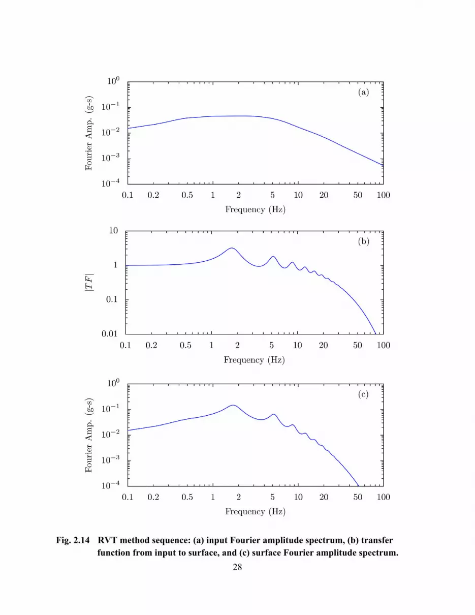
28
Fig. 2.14 RVT method sequence: (a) input Fourier amplitude spectrum, (b) transfer function from input to surface, and (c) surface Fourier amplitude spectrum.

3 Variation of Site Properties
3.1 INTRODUCTION
A soil profile consists of discrete layers that vary in thickness based on the properties of the soil.
The layers are typically discretized based on the soil type, recorded from borehole samples or
inferred from a shear-wave velocity profile. In seismic site response analysis, each layer is
characterized by a thickness, mass density, shear-wave velocity, and nonlinear properties
(G/Gmax, and D). One of the challenges in defining values for these properties is the natural
variability across a site and the uncertainty in their measurement. Because the dynamic response
of a site is dependent on the soil properties, any variation in the soil properties will change both
the expected surface motion and its standard deviation.
In a simple system, the variability of the components can be analytically combined to
quantify the variability of the complete system, thus allowing for the expected value and
variability of the system response to be computed. In seismic site response analysis, the
nonlinear response of the system does not allow an exact analytic quantification of the variability
of the site response. Instead, an estimate of the expected surface response and its standard
deviation due to variations in the soil properties can be made through Monte Carlo simulations.
Monte Carlo simulations estimate the response of a system by generating parameters of the
system based on defined statistical distributions and computing the response for each set of input
parameters. The following chapter introduces Monte Carlo simulations as applied to site
response analysis and presents the models that describe the variability of the layering, shear-
wave velocity, and nonlinear properties (G/Gmax, and D).
3.2 RANDOM VARIABLES
The goal of a Monte Carlo simulation is to estimate the statistical properties of the response of a
complex system. To achieve this goal, each of the properties of the system is selected from
defined statistical distributions and the response of the system is computed. The response is

30
computed for many realizations and the calculated response from each realization is then used to
estimate statistical properties of the system's response. While Monte Carlo simulations can be
used on a wide variety of problems, a major disadvantage is that a large number of simulations is
required to achieve stable results.
Monte Carlo simulations require that each of the components in the system has a
complete statistical description. The description can be in the form of a variety of statistical
distributions (i.e., uniform, triangular, normal, log-normal, exponential, etc.); however the
normal and log-normal distributions typically are used because they can be easily described
using a mean (μ) and a standard deviation (σ). For normally distributed variables, a random value
(x) can be generated by:
= + x xx μ σ ε (3.1)
where μx is the mean value, σx is the standard deviation, and ε is a random variable with zero
mean and unit standard deviation. Random values of ε are generated and used to define the
random values of x.
To generate multiple random variables that are independent, Equation 3.1 can be used for
each variable with different, random values of ε generated for each variable. In the case of
correlated random variables, a more complicated procedure is required for the generation of
values. The correlation between variables is quantified through the correlation coefficient (ρ).
The correlation coefficient can range from -1 to 1. Uncorrelated variables have ρ=0 (Fig. 3.2a).
Positive correlation between variables indicates that the two variables have a greater tendency to
both differ from their respective mean values in the same direction (Fig. 3.1b). As ρ approaches
1.0, this correlation becomes stronger. Negative correlation indicates that variables have a
greater tendency to differ in the opposite direction (Fig. 3.2c).

31
Fig. 3.1 Two variables with correlation coefficient of (a) 0.0, (b), 0.99, and (c) -0.7.
As discussed previously, independent random variables from a normal distribution are
generated by applying Equation (3.1) independently to each random variable. By combining the
multiple applications of Equation (3.1) into a system of equations, the generation of two
independent variables is achieved by multiplying a vector of random variables (ε ) by a matrix
([σ]) and adding a constant ( μ ), defined as:
1
2
x1 1 1
2 2 2
0 = + 0 x
xx
σ ε με μσ
⎡ ⎤⎧ ⎫ ⎧ ⎫ ⎧ ⎫⎢ ⎥⎨ ⎬ ⎨ ⎬ ⎨ ⎬⎢ ⎥⎩ ⎭ ⎩ ⎭ ⎩ ⎭⎣ ⎦
(3.2)
where ε1 and ε2 are random variables randomly selected from a standard normal distribution (μ =
0 and σ = 1), σx1 and σx2 and are the standard deviations of x1 and x2, respectively, and μ1 and μ2
are the mean values of x1 and x2, respectively. Because the random variables x1 and x2 are
independent (ρx1,x2 = 0), the off-diagonal values in the matrix ([σ]) are zero.
Using the same framework, a linear system of equations is used to generate a pair of
correlated random variables. However, the off-diagonal values in the matrix can no longer be
zero because of the correlation between X1 and X2. Instead, a pair of correlated random variables
( x ) is generated by (Kao 1997):
1
21 2 2
0
x1 1 1
,2 2 21 2
2 = + 1xx x x
xx xx
σ ε μσρ σ ε μρ
⎡ ⎤⎧ ⎫ ⎧ ⎫ ⎧ ⎫⎪ ⎪ ⎪ ⎪ ⎪ ⎪⎢ ⎥⎨ ⎬ ⎨ ⎬ ⎨ ⎬⎢ ⎥⎪ ⎪ ⎪ ⎪ ⎪ ⎪⎩ ⎭ ⎩ ⎭ ⎩ ⎭⎢ ⎥⎣ ⎦
− (3.3)

32
Here, the first random variable (x1) is calculated based on the value of ε1 alone, while the second
random variable (x2) is a function of both ε1 and ε2. Note that ε1 and ε2 still represent random and
independent variables generated from the standard normal distribution.
3.3 STATISTICAL MODELS FOR SOIL PROPERTIES
For the properties of the soil to be randomized and incorporated into Monte Carlo simulations,
the statistical distribution and properties of the soil need to be characterized. In this research, two
separate models are used. The first model, developed by Toro (1995), describes the statistical
distribution and correlation between layering and shear-wave velocity. The second model by
Darendeli (2001) was previously introduced in Section 2.1.3 and is used to describe the statistical
distribution of the nonlinear properties (G/Gmax, and D).
3.3.1 Layering and Velocity Model
In Strata, the randomization of the layering and the shear-wave velocity are done through the use
of the models proposed by Toro (1995). The Toro (1995) models provide a framework for
generating layering and then to vary the shear-wave velocity of these layers. The model for
shear-wave velocity variation improves upon previous work by quantifying the correlation
between the velocities in adjacent layers. In previous models, one of two assumptions were made
that simplified the problem: the velocities at all depths are perfectly correlated and can be
randomized by applying a constant random factor to all velocities (McGuire et al. 1989; Toro et
al. 1992), or the velocities within each of the layers are independent of each other, and therefore
can be randomized by applying an independent random factor to each layer (Costantino el al.
1991). While these two assumptions simplify the problem, they represent two extreme
conditions. The Toro (1995) model makes neither of these assumptions; instead the model
incorporates correlation between layers.

33
3.3.1.1 Layering Model
The layering is modeled as a Poisson process, which is a stochastic process with events occurring
at a given rate (λ). For a homogeneous Poisson process this rate is constant, while for a non-
homogeneous Poisson process the rate varies. Generally, a Poisson process models the
occurrence of events over time, but for the layering problem the event is a layer interface and its
rate is defined in terms of length (i.e., number of layer interfaces per meter).
In the Toro (1995) model, the layering thickness is modeled as a non-homogeneous
Poisson process where the rate changes with depth (λ(d), where d is depth from the ground
surface). Before considering the non-homogeneous Poisson process, first consider the simpler
homogeneous Poisson process with a constant rate. For a Poisson process with a constant
occurrence rate (λ), the distance between layer boundaries, also called the layer thickness (h),
has an exponential distribution with rate λ. The probability density function of an exponential
distribution is defined as (Ang and Tang 1975):
( ) ( )exp , 0
; = 0, 0
h hf h
h
λ λλ
− ≥
< (3.4)
The cumulative density function for the exponential distribution is given by:
( ) ( )1 exp , 0
; = 0, 0
h hF h
h
λλ
− − ≥⎧ ⎫⎪ ⎪⎨ ⎬
<⎪ ⎪⎩ ⎭ (3.5)
A random layer thickness with an exponential distribution is generated by solving
Equation (3.5) with respect to thickness (h):
( ) ( )1n 1
= , for 0 < 1F h
h F hλ
−⎡ ⎤⎣ ⎦ ≤−
(3.6)
By randomly generating probabilities (F(h)) with a uniform distribution between 0 and 1
and computing the associated thicknesses with Equation (3.6), a layering profile was simulated
for 10 layers with λ=1 (Fig. 3.2). An exponential distribution with λ=1 will be referred to as a
unit exponential distribution.

34
Fig. 3.2 Ten-layer profile modeled by homogeneous Poisson process with λ = 1.
Another way to think about generating exponential variables with a specific rate is to first
generate a series of random variables with a unit exponential distribution and then convert them
to a specific rate by dividing by the rate [see Eq. (3.6)]. This process is shown in Figure 3.3;
transforming from a constant rate of λ=1 to a constant rate of λ= 0.2. Figure 3.3 and the
associated layering are shown in Figure 3.4. In this example, the thicknesses (and depth) for
λ=1.0 (unit rate) are transformed to thicknesses (and depth) for λ = 0.2 (transformed rate). Here,
each thickness is increased by a factor of 5.0 (1/λ). A similar technique is used to transform
random variables generated with a unit exponential distribution into a non-homogeneous Poisson
process.

35
Fig. 3.3 Transforming from constant rate of = 1 to constant rate of = 0.2.
Fig. 3.4 Ten-layer profile modeled by homogeneous Poisson process with = 0.2.
For a non-homogeneous Poisson process with rate λ(d), the cumulative rate (Λ(d)) is
defined as (Kao 1997):
( ) ( )a
0d = s dsλΛ ∫ (3.7)

36
Λ(d) represents the expected number of layers up to a depth d. To understand the
cumulative rate, consider a homogeneous Poisson process with a constant rate λ (i.e., λ(s) = λ).
In this case, Equation (3.7) simplifies to Λ(d) = λd . For λ = 1.0 (unit rate), Λ(d) = λd such that
the expected number of layers is simply equal to the depth. For λ = 0.2 (transformed rate), Λ(d)
= 0.2⋅d , such that the expected number of layers is one-fifth the value of the unit rate because the
layers are five times as thick. This warping of the unit rate into a constant rate of 0.2 is
represented by the straight line shown in Figure 3.3.
Transforming between the y-axis and x-axis in Figure 3.3 requires the inverse of the
cumulative rate function. For the homogeneous case, Λ-1(u) = u/λ, where u is the depth from an
exponential distribution with λ = 1.0. For the non-homogeneous case, the inverse cumulative
rate function is used to convert from a depth profile for λ = 1.0 (generated by a series of unit
exponential random variables, u) to depth profile with a depth-dependent rate. Before Λ-1(u) can
be defined for the non-homogeneous process, Λ(d) and λ(d) must be defined.
Toro (1995) proposed the following generic depth-dependent rate model:
( ) ( )cd = a d + bλ i
(3.8)
The coefficients a, b, and c were estimated by Toro (1995) using the method of
maximum likelihood applied to the layering measured at 557 sites, mostly from California. The
resulting values of a, b, and c are 1.98, 10.86, and -0.89, respectively. The occurrence rate (λ(d))
quickly decreases as the depth increases (Fig. 3.5a). This decrease in the occurrence rate
increases the expected thickness of deeper layers. The expected layer thickness (h) is equal to the
inverse of the occurrence rate (h = 1/λ(d)) and is shown in Figure 3.5b. The expected thickness
ranges from 4.2 m at the surface to 59 m at a depth of 200 m.
Using Equations (3.7) and (3.8), the cumulative rate for the Toro (1995) modeled is
defined as:
( ) ( ) ( ) 1 1
= s + b = 1 + 1
c cca
0
d b bd a ds ac c
+ +⎡ ⎤+Λ −⎢ ⎥
+⎢ ⎥⎣ ⎦∫ i i (3.9)
The inverse cumulative rate function is then defined as:

37
( )
11c+1cu uu = + + b b
a ac+−1 ⎛ ⎞Λ −⎜ ⎟
⎝ ⎠ (3.10)
Using this equation a homogeneous Poisson process with λ=1.0 (FIG. 3.2) can be warped
into a non-homogeneous Poisson process as shown in Figure 3.6. The resulting depth profile is
shown in Figure 3.7.
Fig. 3.5 Toro (1995) layering model: (a) occurrence rate (λ) as function of depth (d), and (b) expected layer thickness (h) as function of depth.

38
Fig. 3.6 Transformation between homogeneous Poisson process with rate 1 to the Toro (1995) non-homogeneous Poisson process.
Fig. 3.7 Layering simulated with non-homogeneous Poisson process defined by Toro (1995).

39
3.3.1.2 Velocity Model
After the layering of the profile has been established, the shear-wave velocity profile can be
generated by assigning velocities to each layer. In the Toro (1995) model, the shear-wave
velocity at mid-depth of the layer is described by a log-normal distribution. The standard normal
variable (Z) of the ith layer is calculated by:
( )median
1n
1n 1nZ =
s
i ii
v
V V dσ
− ⎡ ⎤⎣ ⎦ (3.11)
where Vi is the shear-wave velocity in the ith layer, Vmedian(di) is the median shear-wave velocity
at mid-depth of the layer, and σlnVs is the standard deviation of the natural logarithm of the shear-
wave velocity. Equation (3.11) is then solved for the shear-wave velocity of the ith layer (Vi):
( ){ }= exp + si lnv i median iV Z ln V dσ ⎡ ⎤⎣ ⎦i (3.12)
Equation (3.12) allows for the calculation of the velocity within a layer for a given
median velocity at the mid-depth of the layer, standard deviation, and standard normal variable.
In the model proposed by Toro (1995), values for median velocity versus depth (Vmedian(di)) and
standard deviation (σlnVs) are provided based on site class. However, in the implementation of the
Toro (1995) model in Strata, the median shear-wave velocity is defined by the user.
Additionally, Strata includes the ability to truncate the velocity probability density function by
specifying minimum and maximum values. The standard normal variable of the ith layer (Zi) is
correlated with the layer above it, and this interlayer correlation is also dependent on the site
class. The standard normal variable (Zi) of the shear-wave velocity in the top layer (i=1) is
independent of all other layers and is defined as:
1 1= Z ε
(3.13)
where ε1 is an independent normal random variable with zero mean and a unit standard deviation.
The standard normal variables of the other layers in the profile are calculated by a recursive
formula, defined as:
21 i = + 1i iZ Zρ ε ρ− −
(3.14)

40
where Zi-1 is the standard normal variable of the previous layer, ε1 is a new normal random
variable with zero mean and unit standard deviation, and ρ is the interlayer correlation.
Correlation is a measure of the strength and direction of a relationship between two
random variables. The interlayer correlation between the shear-wave velocities proposed by Toro
(1995) is a function of both the depth of the layer (d) and the thickness of the layer (h):
( ) ( ) ( ) ( ), = 1 + d h dt h d h dρ ρ ρ ρ−⎡ ⎤⎣ ⎦ (3.15)
where is the thickness-dependent correlation and is the depth-dependent correlation. The
thickness-dependent correlation is defined as:
( ) 0 = exph h
hρ ρ −⎛ ⎞⎜ ⎟Δ⎝ ⎠
(3.16)
where ρ0 is the initial correlation and Δ is a model fitting parameter. As the thickness of the layer
increases, the thickness-dependent correlation decreases. The depth-dependent correlation (ρd) is
defined as a function of depth (d):
( )( )0
2000
200
200200
, > 200
b
d
d d,d
d = d d
ρρ
ρ
⎧ +⎡ ⎤⎪ ≤⎢ ⎥+⎨ ⎣ ⎦⎪⎩
(3.17)
where ρ200 is the correlation coefficient at 200 m and d0 is an initial depth parameter.
As the depth of the layer increases, the depth-dependent correlation increases. The final
layer in a site response model is assumed to be infinitely thick; therefore the correlation between
the last soil layer and the infinite half-space is only dependent on ρd. Toro (1995) evaluated each
of the parameters in the correlation models (ρ0, ρ200, Δ, d0, b) for different generic site classes.
A site class is used to categorize a site based on the shear-wave velocity profile and/or
local geology. In the Toro (1995) model, the statistical properties of the soil profile (the median
velocity, standard deviation, and layer correlation) are provided for two different classifications
schemes, the GeoMatrix and Vs30 classifications. The GeoMatrix site classification classifies
sites based on a general description of the geotechnical subsurface conditions, distinguishing
generally between rock, shallow soil, deep soil, and soft soil (Table 3.1). In contrast, the Vs30 site
classification is based on the time-weighted average shear-wave velocity of the top 30 m (Vs30)
(Table 3.2), and requires site-specific measurements of shear-wave velocity.

41
Toro (1995) computed the statistical properties of the profiles for both the GeoMatrix and
Vs30 classifications using a maximum-likelihood procedure. The procedure used a total of 557
profiles, with 541 profiles for the Vs30 USGS classification and only 164 profiles for the
GeoMatrix classification. The correlation parameters (ρ0, ρ200, Δ, d0, b) are presented in Table
3.3 and the median shear-wave velocities in are presented in Table 3.4.
Table 3.1 Categories of geotechnical subsurface conditions (third letter) in GeoMatrix site classification Toro (1995).
Designation Description A Rock
Instrument is found on rock material (Vs > 600 m/s) or a very thin veneer (less than 5 m) of soil overlying rock material.
B Shallow (Stiff) Soil Instrument is founded in/on a soil profile up to 20 m thick overlying rock material, typically a narrow canyon, near a valley edge, or on a hillside.
C Deep Narrow Soil Instrument is found in/on a soil profile at least 20 m thick overlying rock material in a narrow canyon or valley no more than several kilometers wide.
D Deep Broad Soil Instrument is found in/on a soil profile at least 20 m thick overlaying rock material in a broad canyon or valley.
E Soft Deep Soil Instrument is found in/on a deep soil profile that exhibits low average shear-wave velocity (Vs < 150 m/s).
Table 3.2 Site categories based on Vs30 [Toro (1995)].
Average Shear-wave Velocity Vs30 greater than 750 m/s Vs30 =360 to 750 m/s Vs30 =180 to 360 m/s Vs30 less than 180 m/s

42
Table 3.3 Coefficients for Toro (1995) model.
GeoMatrix Vs30 (m/s) Property A &B C&D >750 360 to
750 180 to
360 < 180
σlnvs 0.46 0.38 0.36 0.27 0.31 0.37 ρ0 0.96 0.99 0.95 0.97 0.99 0.00 ρ200 0.96 1.00 0.42 1.00 0.98 0.50 Δ 13.1 8.0 3.4 3.8 3.9 5.0 d0 0.0 0.0 0.0 0.0 0.0 0.0 b 0.095 0.160 0.063 0.293 0.344 0.744 Profiles 45 109 35 169 226 27
Table 3.4 Median shear-wave velocity (m/s) based on generic site classification.
GeoMatrix Vs30 (m/s) Depth (m) A &B C&D >750 360 to
750 180 to
360 < 180
0 192 144 314 159 145 176 1 209 159 346 200 163 165 2 230 178 384 241 179 154 3 253 193 430 275 191 142 4 278 204 485 308 200 129 5 303 211 550 337 208 117 6 329 217 624 361 215 109
7.2 357 228 703 382 226 106 8.64 395 240 789 404 237 109 10.37 443 253 880 433 250 117 12.44 502 270 973 467 269 130 14.93 575 291 1070 501 291 148 17.92 657 319 1160 535 314 170 21.5 748 357 1260 567 336 192 25.8 825 402 1330 605 372 210 30.96 886 444 1380 654 391 229 37.15 942 474 1420 687 401 246 44.58 998 495 1460 711 408 266 53.2 1060 516 1500 732 413 289 64.2 541 749 433 318 77.04 566 772 459 353 92.44 593 802 486 392 110.93 847 513 435 133.12 900 550 159.74 604 191.69 676 230.03 756

43
Ten generated shear-wave velocity profiles were created for a deep, stiff alluvium site
using the two previously discussed methods. In the first method, a generic site profile is
generated by using the layering model coefficients and median shear-wave velocity for a Vs30 =180 = 180 to 360 m/s site class, shown in Figure 3.8(a). This approach essentially models the
site as a generic stiff soil site. The second method uses the layer correlation for the Vs30 =180 to
360 m/s site class, but the layering and the median shear-wave velocity profile are defined from
field measurements, shown in Figure 3.8(b). The site-specific layering tends to be much thicker
than the generic layering as a result of the field measurements indicating thick layers with the
same shear-wave velocity. In general both of the methods show an increase in the shear-wave
velocity with depth. However, the site-specific shear-wave velocity values are significantly
larger than the generic shear-wave velocity values. At the surface, the generic site has a median
shear-wave velocity of 150 m/s compared to the site-specific shear-wave velocity of 200 m/s. At
a depth of 90 m, the difference is even greater, with the generic site having a median shear-wave
velocity of 470 m/s compared to the site-specific median shear-wave velocity of 690 m/s. The
difference in shear-wave velocity is a result of the difference between the site-specific
information and the generic shear-wave velocity profile.

44
Fig. 3.8 Ten generated shear-wave velocity (vs) profiles for USGS C site class: (a) using generic layering and median vs and (b) using user-defined layering and median vs.
3.3.2 Depth to Bedrock Model
The depth to bedrock can be modeled using either a uniform, normal, or log-normally distributed
random variable. When using the normal or log-normal distribution, the median depth is based
on the soil profile. The variation in the depth to bedrock is accommodated by varying the height
of the soil layers. If the depth to bedrock is increased, then the thickness of the deepest soil layer
is increased. Conversely, if the depth to bedrock is decreased then the thickness of this deepest
soil layer is decreased. If the depth to bedrock is less than the depth to the top of a soil layer, then
the soil layer is removed from the profile.

45
3.3.3 Nonlinear Soil Properties Model
The Darendeli (2001) empirical model for nonlinear soil properties (G/Gmax and D) was
previously discussed in Section 2.1.3. The Darendeli (2001) empirical model assumes the
variation of the properties follows a normal distribution. The standard deviation of G/Gmax and D
varies with the magnitude of the property and is calculated with Equations (2.20) and (2.21),
respectively. Because the variation of the properties is modeled with a normal distribution that is
continuous from -∞ to ∞, the generated values of G/Gmax or D may fall below zero. The most
likely location for the negative values occurs when the mean value is small, which occurs at
large strains for G/Gmax and at low strains for D. Negative values for either G/Gmax or D are not
physically possible; therefore the normal distributions need to be truncated. To correct for this
problem, minimum values for G/Gmax and D are specified. The default values in Strata are
G/Gmax = 0.05 and D = 0.1%. Strata also includes the ability to specify maximum values of
G/Gmax and D.
G/Gmax and D curves are not independent. Consider a soil that behaves more linearly, that
is to say that the G/Gmax is higher than the mean G/Gmax. During a loading cycle, the area inside
the hysteresis loop would be smaller, which is indicative of less damping within the system.
Therefore, as the linearity of the system increases, the damping decreases. To capture this effect,
the soil properties are assumed to have a negative correlation with the default value set at -0.5
(i.e., ρ=-0.5).
To generate correlated G/Gmax and D curves from baseline (mean) curves, the following
expressions are used for each shear strain value in the curves:
( ) ( )/ 1 NGmax max meanG G = G/G + γ γ ε σ⎡ ⎤⎣ ⎦ i (3.18)
( ) ( ) 21 2 = + + 1 D Dmean
D Dγ γ ρ σ ε σ ρ ε−⎡ ⎤⎣ ⎦ i i i i (3.19)
where ε1 and ε2 are uncorrelated random variables with zero mean and unit standard deviation,
[G/Gmax (γ)] and [D(γ)]mean are the baseline values evaluated at strain level γ, σ NG and σ D are the
standard deviations computed from Equations (2.20) and (2.21) at the baseline values of [G/Gmax
(γ)]mean and [D(γ)]mean, respectively, and ρ is the correlation coefficient between G/Gmax and D.
Equations (3.18) and (3.19) must be applied at different strain levels, but the same values of ε1

46
and ε2 are used at each strain level (i.e., perfect correlation between strain levels).
Using a correlation coefficient of -0.5, the nonlinear properties of sand (PI=0, OCR=0) at
a confining pressure of 1 atm were generated 10 times, shown in Figure 3.9. Three of the
realizations result in large shear modulus reduction curve relative to the mean. Because of the
negative correlation, the relatively high shear modulus reduction corresponds to a relatively low
damping ratio.
Fig. 3.9 Generated nonlinear properties assuming perfect negative correlation.

4 Using Strata
Strata is introduced through two examples that demonstrate the program's organization and most
of its features. Before these examples are discussed, some particular differences between Strata
and other site response programs are introduced.
With the exception of acceleration time-series, all of the input to Strata is entered via the
keyboard, or through copying and pasting from spreadsheets. The input file is not saved in the
typical text format; instead a binary format is used that is only readable by Strata. Furthermore,
when the calculation is complete no output text files are produced. Instead, the output can be
directly viewed with Strata and saved, once again to a binary format. An option is provided for
the data to be exported to text files that can then be opened with a variety of applications,
including Excel.
4.1 STRATA PARTICULARS
4.1.1 Auto-Discretization of Layers
One of the biggest differences between Strata and other site response analysis programs is the
fact that the sublayers used in the calculation portion of the analysis are not defined by the user.
Instead, the user defines a velocity layer that is then subdivided into sublayers by Strata. This
fundamental difference exists because Strata allows for the layering and shear-wave velocity to
vary (see Section 3.3.1.1), and therefore the required thickness of the sublayers changes.
The maximum thickness (hmax,i) of the sublayers of ith velocity layer is taken as a fraction
of the minimum wavelength to be captured by the analysis:
,max, frac min frac
max
= s ii
vh
fλ λ λ=
(4.1)
where λfrac is the wavelength fraction which typically varies between 1/10 and 1/5 (anything
greater than 1/3 is not recommended), fmax is the maximum frequency of engineering interest
which is typically around 20 Hz, and vs,i is the shear-wave velocity of the ith layer. The actual

48
thickness of the sublayers is less than the maximum thickness such that the velocity layer height
divided by the sublayer thickness is a whole number. These parameters are defined on the
General Settings tab. To prevent the layers from being auto-discretized, the wavelength fraction
can be increased and the thickness of the velocity layers defined in the Soil Profile tab can be
selected to represent the actual layer thickness used in the analysis. This approach is the same as
used in most site response programs.
In other site response programs, the location of the input motion or the location of
requested output (e.g., acceleration time history) is generally referenced by a sublayer index.
However, because the sublayers are computed in Strata (and may change for each realization),
the location is defined in terms of the depth within the soil profile or at the top of the bedrock.
When the location is specified as Bedrock, then the actual depth of the location may change if
the depth of the bedrock changes. The location is specified with a drop-down list shown in
Figure 4.1, where the user can specify the depth as Bedrock (Fig. 4.1a) or a fixed depth (Fig.
4.1c).
Fig. 4.1 Location selection: (a) top of bedrock, (b) switching to fixed depth, and (c) fixed depth specified as 15.
4.1.2 Interaction with Tables
Table cells are selected with one click. After a cell is selected, the cell can be edited by typing. A
cell's edit mode can be directly entered by double clicking on the cell. In some cases, double
clicking on a cell will produce a widget to aid specifying input to the cell.
All tables used in Strata are dynamic; that is, the number of rows can be changed. Rows
are added to the bottom of the list with the Add button. The Insert and Remove buttons are
disabled until a complete row has been selected, which is most easily achieved by clicking on the
number next to the row of interest. Multiple continuous rows can be selected by pressing the
shift key while selecting the rows. After rows have been selected: Add will add the same number
of rows to the end of the table, Insert will insert the same number of rows above the currently

49
selected rows, and Remove will remove the selected rows. All rows in the table can be selected
by clicking on the button in the upper right portion of the table as shown in Figure 4.2. Some
tables have cells that cannot be edited and have a light gray background (Fig. 4.2).
Fig. 4.2 By clicking on button circled in red, all rows in table are selected.
Data can be copied from spreadsheets and pasted into tables by first clicking on the table
and:
1. Pressing Ctrl+v, or
2. Selecting Paste from the Edit menu in Strata, or
3. Right clicking on the table and selecting paste.
The table will automatically increase the numbers of rows to accommodate the size of the
pasted data.
4.1.3 Nonlinear Curves
The nonlinear shear-modulus reduction and damping curves can be specified through three
different methods in Strata: (1) fixed models that are present by default and cannot be removed,
(2) user-defined curves that can be used across projects, and (3) temporary models that exist only
for the project.

50
Fixed Nonlinear Models
The following shear-modulus reduction models are included by default:
• Darendeli (2001)
• EPRI (1993)
• Plasticity Based: 10, 30, 50, and 70
• Depth Based: 0–20, 20–50, 50–120, 120–250, 250–500, and 500–1000 ft
• GEI (1993): 0–50, 50–100, 100–250, 250–500, and >500 ft
• GeoMatrix (Coppersmith 1991): 0–50, 50–150, and >150 ft
• Idriss (1990): clay and sand
• Imperial Valley Soils (Turner and Stokoe 1983): 0–300 and >300 ft
• Iwasaki (1976): 0.25 and 1.0 atm
• Peninsular Range (Silva et al. 1997): 0–50 and 50–500 ft
• Seed and Idriss (1970): sand lower, mean, and upper
• Vucetic and Dobry (1991): Plasticity indices of 0, 15, 30, 50, 100, and 200
User-Defined Models
Nonlinear curve models can be defined for use across multiple projects by adding models to the
library. The nonlinear property manager is opened by selecting Add/Remove Non-Linear
Property Curves from the Tools menu. Using the dialog (Fig. 4.3), a new model can be defined
by following these steps:
1. Click the Add button to add a new curve to the normalized shear-modulus reduction or
damping models list.
2. Rename the model from Untitled to something more meaningful.
3. Add the data points to the curve.
Models defined in this manner will be added to the nonLinearCurves.strd file found in the
Strata installation folder.

51
Fig. 4.3 Nonlinear curve manager.
Temporary Models
If you want to define a curve without adding it to the library of models, simply select Custom
from the drop-down list in the Soil Types table. Changing to the Custom model does not clear
the previous model’s data, which allows for a model to be modified.
2

52
4.1.4 Recorded Motion Dialog Box
The Recorded Motion dialog box is used to load a recorded motion into Strata and appears when
the Add button is clicked in the Record Motion(s) table within the Motion(s) tab. The dialog box,
shown in Figure 4.4 allows the user to load a variety of motions in most formats using the
following steps:
1. Click on the File button and select the acceleration time-series text file. If the file is from
the NGA database, then the remainder of the form will be automatically completed as
shown in Figure 4.4. Regardless of the file format, the file is read and loaded into the
preview area.
2. The remaining fields need to be filled to reflect the information in the file. Information is
required for all fields except for the Description field. Fields can be completed by either
typing values in, or selecting from the file preview and dragging the selected text into the
field. The Start line and Stop line control which lines in the file contain the data. A zero
value for the Stop line will result in the data being read until the end of the file. The file
preview can be colored by clicking on the Refresh button.
The colors have the following meanings:
• Green: text found prior to the acceleration time-series data (these lines are
ignored).
• Blue: acceleration time-series data.
• Red: text after the time series data (these lines are ignored).
An example of the colored data is shown in Figure 4.5.
3. The scale factor can be selected at this time or after the motion has been loaded. If the
input acceleration time history is not in units of g (g=acceleration of gravity), then the
scale factor should be used to make this unit conversion. After the motion has been
loaded, the scale factor can also be adjusted by assigning a peak-ground acceleration.
4. After the form has been completed, the time-series can be viewed by clicking on the Plot
button.
5. Click OK to finish loading the file.

53
Fig. 4.4 Initial view of Recorded Motion dialog box.
Fig. 4.5 Example of completed Recorded Motion dialog box.
4.1.5 Results Page
Prior to the calculation of the site response, the Results tab is disabled. After the site response
calculation has been completed, the Results tab will be enabled and selected. The remaining tabs
are placed in a read-only (or “locked”) mode where the fields can be reviewed but not edited.
Therefore, the input parameters used to generate the output are strictly linked for later reference
by the user.
Strata can be unlocked by clicking on the open lock icon in the upper left portion of the
screen, by selecting Unlock from the Tools menu, or by pressing F2. By unlocking Strata, all of
the results are deleted. If you wish to save the results and make changes to the input and re-run
the analysis. First, save the results using either the Save or Save As command from the File
menu. Next create a copy of the file by selecting Save As from the File menu and

54
using a new name appropriate for the new input parameters. Finally, unlock the newly created
file.
Strata does not output any data files automatically; instead the results are saved to the
project file in a binary format. To work with the data outside of Strata, the data can be exported
by selecting Export from the File menu. The exported data file is in a comma-separated values
(CSV) format that can easily be opened with Excel or another spreadsheet program. All data
(even disabled results) are included in the files.
A screenshot of the Results tab is shown in Figure 4.6. Each result represents a site
realization subjected to an input motion. The output of interest is selected from a drop-down box
containing a list of all requested output. Individual values from this list are selected by either
clicking on the corresponding row in the Data Selection table or by clicking on the result in the
plot. In both cases, the result is colored green if the result is enabled, or red if disabled. A result
can be enabled or disabled by clicking on the checkbox next to the site realization that produced
the result. After the status of a result has been changed, the Recompute Statistics button will
become enabled indicating that the median and standard deviation (shown on the plot in solid
and dash blue lines, respectively) need to be updated. Click this button to recompute the
statistics.
At the bottom of the table there are two buttons that allow all motions or sites related to
the currently selected result to be enabled or disabled. In the example (Fig. 4.6), the motion
CHICHI06\TCU076-E.AT2 has been disabled. Whenever the status of a result is changed (e.g.,
from disabled to enabled) the Recompute Statistics button will become enabled allowing the user
to update the median and standard deviation. The current plot can be printed by selecting Print or
Print to PDF from the File menu. The current plot can also be copied by right clicking on the plot
and selecting Copy.

55
Fig. 4.6 Using Output view to examine results of calculation.
4.2 GLOSSARY OF FIELDS
The following section contains screenshots of the program and describes each of the fields.
Assume that information is required for each field, unless stated otherwise.

56
4.2.1 General Settings Page
Project Group Box
Fig. 4.7 Screenshot of Project group box.
• Title: name of the project (optional). The title is included in the first row of the exported
data and therefore can be extremely useful in identifying the output.
• Notes: a place to store information about the input (optional); only used to preserve your
sanity.
• Filename prefix: placed at the beginning of the name of all exported files (optional). The
prefix offers a means to distinguish a group of analyses.
• Units: defines gravity in the analysis. Changing the units does not perform any
conversion; it is recommended that the units be defined before any site information is
provided.
• Save motion data checkbox: allows the time series to be saved within the input file
(optional). If checked then the time series information is stored within the input file,
allowing one file to be transferred between computers. However, larger input files will be
generated.

57
Type of Analysis Group Box
Fig. 4.8 Screenshot of Type of Analysis group box.
• Calculation Method: either Recorded Motions for a time series analysis, or Random
Vibration Theory for RVT analysis.
• Vary the properties checkbox: Controls if site properties will be varied in the calculation.
Site Property Variation Group Box
Fig. 4.9 Screenshot of Site Property Variation group box.
This group box is only enabled if the Vary the Properties check box in the Type of Analysis
group box is enabled.
• Number of realizations: number of sites to be generated. A site consists of nonlinear
curves, shear-wave velocity profile, layering thickness, and depth to bedrock The
variation of each of these properties is controlled elsewhere. Each of the input motions is
propagated through a generated site.
• Vary the nonlinear soil properties: controls if the shear modulus reduction and damping
curves are varied.
• Vary the site profile: controls if the velocity, layer thickness, and/or depth to bedrock are
varied.

58
Equivalent-Linear Parameters Group Box
Fig. 4.10 Screenshot of Equivalent-Linear Parameters group box.
Fig. 4.11 Screenshot of Layer Discretization group box.
• Effective strain ratio: the ratio between the effective shear strain (used for the strain-
compatible nonlinear properties) and the maximum shear strain computed in the layer.
• Error tolerance: the maximum error in the nonlinear properties between iterations.
• Maximum number of iterations: if the error tolerance is not achieved in this number of
iterations, the calculation ends.
Layer Discretization Group Box
• Maximum frequency: maximum frequency of engineering interest.
• Wavelength fraction: thickness of the layer relative to the wavelength at the maximum
frequency of engineering interest.

59
4.2.2 Soil Types Page
Soil Types Group Box
Fig. 4.12 Screenshot of Soil Types group box.
• Name: used for indentifying soil layer in the program and output.
• Unit weight: total unit weight of the soil.
• Initial damping: this damping is used during the initial iteration.
• G/G_max Model: model that describes the variation of normalized shear modulus with
shear strain.
• Damping Model: model that describes the variation of the damping ratio with shear
strain.
• Notes: only to assist you (optional).
• Varied: check box to identify if the nonlinear curves of the soil type will be varied.
Visible only if the variation of the nonlinear curves is enabled.
Bedrock Layer Group Box
Fig. 4.13 Screenshot of Bedrock Layer group box.
• Unit weight: total unit weight of the infinite half space.
• Initial damping: damping of the infinite half space.
• Vary the damping of the bedrock: check box to identify if the damping in the bedrock is
to be varied

60
Nonlinear Curve Variation Parameters Group Box
Fig. 4.14 Screenshot of Nonlinear Curve Variation Parameters group box.
• Standard Deviation Model: model to describe the variability of the nonlinear parameters.
• Normalized shear modulus
o Stdev: formula to describe the standard deviation. Enabled if standard deviation
model is set to custom.
o Max: maximum value of the normalized shear modulus reduction.
o Min: minimum value of the normalized shear modulus reduction.
• Damping
o Stdev: formula for the standard deviation. Enabled if standard deviation model is set
to custom.
o Max: maximum value of the damping ratio.
o Min: minimum value of the damping ratio.
• G/G_max, Damping Correlation Coefficient (ρ): correlation coefficient between the
varied nonlinear curves.
Darendeli and Stokoe Model Parameters Group Box
Fig. 4.15 Screenshot of Darendeli and Stokoe Model Parameters group box.

61
This group box is only enabled when a soil type that uses the Darendeli and Stokoe (2001) model
for either of the nonlinear soil properties is selected.
• Mean effective stress: mean effective stress of the soil in units of atmospheres.
• Plasticity index: plasticity index of the soil.
• Overconsolidation ratio: overconsolidation ratio of the soil.
• Excitation frequency: frequency of excitation.
• Number of cycles: number of loading cycles.
Nonlinear Property Group Box
Fig. 4.16 Screenshot of Nonlinear Property group box.
For fixed models, this table will provide a read only view of the data points used in the models.
The values of the models can be edited by switching the model to custom. The second column in
the table changes depending on what type of model is selected in the Soil Type table.
• Strain (%): shear strain in percent.
• G/G_max: normalized shear modulus.
• Damping (%): damping ratio in percent.

62
4.2.3 Soil Profile Page
Velocity Layers Group Box
Fig. 4.17 Screenshot of Velocity Layers group box.
• Depth: depth of the top of the velocity layer: computed by Strata.
• Thickness: thickness of velocity layer.
• Soil Type: Soil Type associated with the velocity layer. This associates the velocity layer
to a specific unit weight and nonlinear properties for the analysis.
• Vs : shear-wave velocity of the layer.
• Minimum: minimum shear-wave velocity. Minimum value of shear-wave velocity
allowed during Monte Carlo simulation.
• Maximum: maximum shear-wave velocity. Maximum value of shear-wave velocity
allowed during Monte Carlo simulation.
• Varied: check box to identify if the shear-wave velocity of the layer is to be varied.
Variation of the Site Profile Group Box
The Variation of the Site Profile group is hidden unless the Vary the Site Profile checkbox is
checked on the General Settings page. For each of the functionalities (shear-wave velocity
variation, layer thickness variation, and depth to bedrock variation), there is a check box that
controls if the functionality should be activated. A group box for model parameters appears for
each functionality when the functionality is enabled.
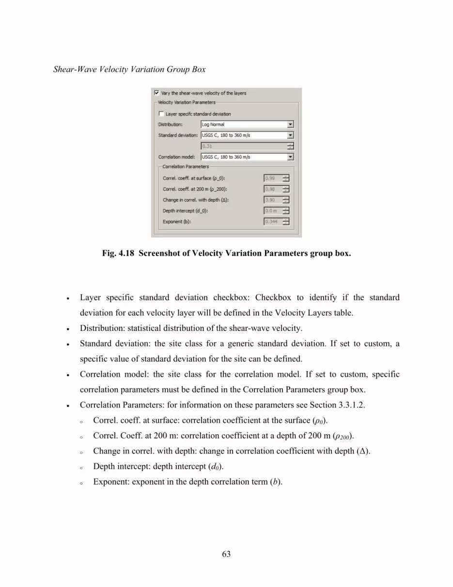
63
Shear-Wave Velocity Variation Group Box
Fig. 4.18 Screenshot of Velocity Variation Parameters group box.
• Layer specific standard deviation checkbox: Checkbox to identify if the standard
deviation for each velocity layer will be defined in the Velocity Layers table.
• Distribution: statistical distribution of the shear-wave velocity.
• Standard deviation: the site class for a generic standard deviation. If set to custom, a
specific value of standard deviation for the site can be defined.
• Correlation model: the site class for the correlation model. If set to custom, specific
correlation parameters must be defined in the Correlation Parameters group box.
• Correlation Parameters: for information on these parameters see Section 3.3.1.2.
o Correl. coeff. at surface: correlation coefficient at the surface (ρ0).
o Correl. Coeff. at 200 m: correlation coefficient at a depth of 200 m (ρ200).
o Change in correl. with depth: change in correlation coefficient with depth (Δ).
o Depth intercept: depth intercept (d0).
o Exponent: exponent in the depth correlation term (b).

64
Layer Thickness Variation Group Box
Fig. 4.19 Screenshot of Layer Thickness Variation group box.
For more information on the parameters in this group box see Section 3.3.1.1.
• Coefficients: the parameters for the model used to vary layer thickness. If set to custom
then the model parameters a, b, and c are defined by the user.
Bedrock Depth Variation Group Box
Fig. 4.20 Screenshot of Bedrock Depth Variation group box.
• Distribution: the statistical distribution of the bedrock depth, either uniform, normal, or
log normal.
• Standard deviation: standard deviation of the log normal or normal distribution. For a log
normal distribution, this value is defined in log space.
• Minimum depth to bedrock: check box to identify if the distribution is to be truncated at a
minimum depth, and associated minimum depth.
• Maximum depth to bedrock: check box to identify if the distribution is to be truncated at
a maximum depth, and associated maximum depth.

65
4.2.4 Motion(s) Page
The Motion page is used to define the input motion(s) and where the input motion(s) is (are)
input into the soil profile. Depending on the type of analysis, the motion(s) are defined in
different ways.
Motion Input Location Group Box
Fig. 4.21 Screenshot of Motion Input Location group box.
• Specify the location to input the motion(s): The input location specifies where the input
motion should be specified. The adjacent box can be used to specify a specific depth or
the bedrock (see Section 4.2). If the input location is defined as bedrock, then the location
will be at the top of the bedrock regardless of the randomized depth of the bedrock.
Recorded Motion(s)
Fig. 4.22 Screenshot of Recorded Motions table.
A recorded motion is added to the table by clicking on the Add button, and filling in the
information in the dialog box (see Section 4.1.4 for more information). The following
information is presented in the Recorded Motion(s) table:

66
• Filename: contains the directory and filename of the motion.
• Description: description of the time series (optional).
• Type: type of boundary conditions of the motion; either Outcrop or Within.
• Scale Factor: scale factor to convert the motion into units of gravity (if required, see
Section 4.1.4) at the desired amplitude. Changing the scale factor changes the listed peak
ground acceleration (PGA) value.
• PGA: the PGA of the record in units of gravity can be specified. Changing this value
changes the listed scale factor.
An entire suite of motions in the NGA (Next Generation Attenuation,
http://peer.berkeley.edu/nga) format can be added by clicking on the Load Suite push button,
which opens a file selection dialog box. The suite file is a simple text file with the extension .csv.
Each line of the file contains the path name to the motion and the scale factor separated by a
comma. The path name can be either absolute or relative to the path of the suite file. If examples
were installed during the installation of Strata, then an example suite file named suite-10-1.csv
can be found in the examples directory.
Random Vibration Theory
When the random vibration theory method is selected a variety of methods can be used to specify
the input motion. Regardless of the method some basic properties must be defined.
Properties
Fig. 4.23 Screenshot of Properties Group box for RVT motion.

67
• Type: type of boundary conditions of the motion; either Outcrop or Within.
• Source: method used to characterize the motion. The following options are available:
o Defined Fourier Spectrum
o Defined Response Spectrum
o Calculated Fourier Spectrum
• Duration: duration of the event (D5-75) (disabled when the source is a calculated Fourier
spectrum).
• Strain factor: the factor to apply to the duration used for the RVT calculation of the strain
(recommended value 1.0).
• Soil factor: the factor to apply to the duration used for the RVT calculation of motion at
the top of the soil column (recommended value 1.0).
• Damping: damping of the response spectrum. This damping is used for both the preview
of the response spectrum and for the input response spectrum.
• Limit FAS shape checkbox: limits the shape of the FAS during the inversion (see Section
2.2.2.4) from response spectrum to Fourier spectrum (enabled only when the source is a
defined response spectrum).
• Data push button: clicking on this push button shows a table of the Fourier amplitude
spectrum and associated response spectrum for the motion.
• Plot push button: clicking on this push button shows a plot of the Fourier amplitude
spectrum and associated response spectrum for the motion.
Fourier Amplitude Spectrum Group Box
Fig. 4.24 Screenshot of Fourier Amplitude Spectrum group box.
The Fourier Amplitude Spectrum group box is used to specify an acceleration Fourier amplitude
spectrum directly. The simplest method of entering data into this table is pasting from a
spreadsheet. The columns represent the following:
• Frequency: frequency in Hertz.
• Fourier Amplitude: Fourier amplitude at the frequency in units of gravity/sec.

68
Acceleration Response Spectrum Group Box
Fig. 4.25 Screenshot of Acceleration Response Spectrum group box.
The Acceleration Response Spectrum group box is used to specify an acceleration response
spectrum that is used to compute a Fourier spectrum through inversion (see Section 2.2.2.4). The
simplest method of entering data into this table is pasting from a spreadsheet. The columns
represent the following:
• Period (s): period of the oscillator in units of seconds.
• Spec. Accel. (g): spectral acceleration of the oscillator in units of gravity.

69
Point Source Model Group
Fig. 4.26 Screenshot of Point Source Model group box used to define input RVT motion using seismological source theory.
Point Source Model Group Box
• Moment Magnitude: moment magnitude of the event.
• Epicentral distance: distance to the epicenter in km.
• Depth: depth to the rupture in km.
• Location: crustal region associated with the source and crustal properties. Choose from
western U.S., central and eastern U.S., and Custom. The western U.S. and central and
eastern U.S. values are from Campbell (2003).
• Stress drop: stress drop of the rupture (required for Custom location).
• Geometric attenuation coeff.: geometric attenuation coefficient. For example, if the

70
geometric attenuation relationship is 1/R and R=20, then this value would be 0.05.
• Path duration coefficient: factor used to define the portion of the duration that is
dependent on the path distance (Tp). See Section 2.2.2.2 for details.
• Path attenuation: frequency dependent path attenuation Q defined by a coefficient (a) and
a power (b) using Q = a fb
• Shear velocity: shear-wave velocity at the rupture in km/s.
• Density: density of the rock at the rupture in g/cm3.
• Site attenuation: site attenuation κo.
• Site-specific crustal amplification: allows for the crustal amplification to be computed for
a site-specific crustal velocity profile using the quarter-wavelength method (Boore 2003).
Enabling this check box requires that the user then define the thickness, shear-wave
velocity, and density of the crustal layers, as shown in Figure 4.27.
Fig. 4.27 Screenshot of Crustal Velocity Model group box.
4.2.5 Output Specification Page
Response Location Output Group Box
Fig. 4.28 Screenshot of Response Location Output group box.
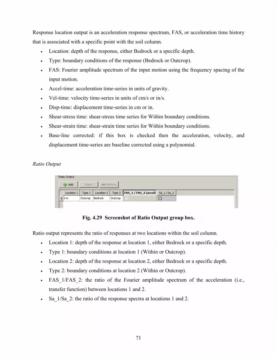
71
Response location output is an acceleration response spectrum, FAS, or acceleration time history
that is associated with a specific point with the soil column.
• Location: depth of the response, either Bedrock or a specific depth.
• Type: boundary conditions of the response (Bedrock or Outcrop).
• FAS: Fourier amplitude spectrum of the input motion using the frequency spacing of the
input motion.
• Accel-time: acceleration time-series in units of gravity.
• Vel-time: velocity time-series in units of cm/s or in/s.
• Disp-time: displacement time-series in cm or in.
• Shear-stress time: shear-stress time series for Within boundary conditions.
• Shear-strain time: shear-strain time series for Within boundary conditions.
• Base-line corrected: if this box is checked then the acceleration, velocity, and
displacement time-series are baseline corrected using a polynomial.
Ratio Output
Fig. 4.29 Screenshot of Ratio Output group box.
Ratio output represents the ratio of responses at two locations within the soil column.
• Location 1: depth of the response at location 1, either Bedrock or a specific depth.
• Type 1: boundary conditions at location 1 (Within or Outcrop).
• Location 2: depth of the response at location 2, either Bedrock or a specific depth.
• Type 2: boundary conditions at location 2 (Within or Outcrop).
• FAS_1/FAS_2: the ratio of the Fourier amplitude spectrum of the acceleration (i.e.,
transfer function) between locations 1 and 2.
• Sa_1/Sa_2: the ratio of the response spectra at locations 1 and 2.

72
4.3 EXAMPLES
The following examples give a basic introduction for using Strata to perform equivalent-linear
site response analysis. Each of the examples and required acceleration time-series can be
installed by including the examples option during installation. The example files are found
within the examples folder in the installation path (e.g., C:\Program Files\Strata\examples) or by
the shortcut in the Strata start manual folder. The examples can be opened by either double
clicking on the file or by selecting them from Open in the File menu.
All examples use the deep alluvium Sylmar County Hospital Parking Lot (SCH) site
located in Southern California for the site profile. The soil types and velocity layering of the site
were proposed by Chang (1996). The soil properties are listed in Table 4.1, with a water table at
a depth of 46 m. The nonlinear properties for each of the layers were computed using the
Darendeli (2001) empirical model with PI=0, OCR=1, and the confining pressures listed in Table
4.1. The corresponding velocity profile is shown in Figure 4.30 (Chang 1996). The minimum and
maximum values are those recommended in Chang (1996). The time-averaged shear-wave
velocity over the top 30 m was computed as 273 m/s.
Table 4.1 Soil profile at Sylmar County Hospital Parking Lot site (Chang 1996). Mean effective stress ( ) computed assuming k0 of 1/2 and water table depth of 46 m.
Depth Range (m) Soil Type
Vs (m/s)
γtotal
(kN/m3)νσ ′
(kPa) mσ ′
(atm)0 to 6 Alluvium (Sand) 200 (150 to 230) 18 54 0.36 6 to 31 Alluvium (Sand) 300 (240 to 350) 18 222 2.2 31 to 61 Alluvium (Sand) 460 (370 to 550) 19 562 5.6
61 to 91 Alluvium and Older Alluvium (Sand) 700 (580 to 750) 22 776 7.7
91+ Bedrock 760 22

73
Fig. 4.30 Shear-wave velocity profile of Sylmar County Hospital Parking Lot site (Chang 1996).
4.3.1 Example 1: Basic Time Domain
In the first example, the site response is computed for the Sylmar County Hospital Parking Lot
site using a single acceleration time-series. The input file for this example is named example-1-
td.strata. In this example, the steps required to compute the acceleration response spectrum at the
surface of the site are presented. The following steps assume that you are working from a new
project.
4.3.1.1 General Settings Page
For the most part, the default values are acceptable on the General Settings page, but a few
options need to be defined more carefully:
(1) A title should be created that accurately represents the project; this example uses Sylmar
County Hospital Site: Time domain.
(2) The default unit system in Strata is the metric system. The units specified on the General
Settings page must be in agreement with the units used throughout the input file.
(3) The default calculation method is Recorded Motions, which is used for this example.

74
4.3.1.2 Soil Types Page
The information presented regarding the site information (Table 4.1 and Fig. 4.30) is input into
Strata in two different steps. First, the Soil Types page is used to define the soil types found
within the profile. These soil types are then spatially arranged in the Soil Profile page. The
following steps are required to define the Soil Types for the Sylmar County Hospital site:
(1) In the Soil Types table, click the Add button to create a new soil type, and enter the
information found in Table 4.1. The initial damping is the damping in the soil used for
the first equivalent-linear iteration and 5% is appropriate for most cases. The nonlinear
property model is selected from a drop-down list. Select the Darendeli (2001) nonlinear
model for both the shear modulus reduction and the damping curves.
(2) Additional information regarding the soil type is required for the Darendeli (2001)
nonlinear model and is found within the Darendli and Stokoe Model Parameters group
box. The soil is an alluvium with a plasticity index of 0 and an overconsolidation ratio of
1, which are the default values for the PI and OCR. The excitation frequency and number
of cycles will also be left at the default values (1 Hz and 10, respectively). The Darendeli
(2001) model requires the mean effective stress for the soil, which is 0.36 atm for the
center of the top alluvium layer.
(3) Repeat steps (1) and (2) for the remaining three soil types.
(4) The bedrock layer is defined by a unit weight of 22 kN/m3 and damping of 1%.

75
4.3.1.3 Soil Profile Page
The Soil Profile page is used to spatially arrange the soil types and to define the shear-wave
velocity associated with each layer. The following steps are used to input the soil profile
information:
(1) In the Velocity Layers table, click on the Add button to create a new soil profile layer.
(2) Define the thickness (6 m), soil type (Alluvium (0.36 atm)), and shear-wave velocity (200
m/s) of the layer.
(3) Repeat steps (1) and (2) until all of the layers are defined.
4.3.1.4 Motion(s) Page
For this example, the site response analysis is being computed for one recorded motion. This
motion is loaded using the following steps:
(1) The motion will be input at the top of the bedrock, so the default location to input the
motion is correct.
(2) The motion is loaded by clicking on the Add button in the Recorded Motion(s) table. This
will open a dialog box that assists in loading the file (see Section 4.1.4). Click on the File
button in the upper left portion of the dialog box and select the VAS090.AT2 file from
the NORTHR directory (depending on where you installed Strata, this might be
“C:\Program Files\Strata\example\motions\NORTHR”). Strata automatically parses the
AT2 file and fills in the required information. For motions not in the AT2 format, all of
the boxes need to be filled in by hand.

76
(3) Click on the OK button to complete the loading of the file.
4.3.1.5 Output Specification Page
In this example, the goal is compute the acceleration response spectrum at the surface of the site.
The requested output will also include the shear strain profile, the acceleration response spectrum
at the bedrock, and the spectral ratio between the surface and input rock motions.
(1) For the acceleration-response spectrum, click on the Add button in the Response
Location Output table. Assign the location of the layer to be at the surface (0 m) and
select an outcrop boundary condition. Next, click on the check box in the Accel. Resp.
Spec. column.
(2) To obtain the input acceleration response spectrum at the bedrock level, click on the Add
button to generate another Response Location. For this row, use the drop-down box in the
location column to set the depth Bedrock, and select the Outcrop boundary condition.
(3) For the spectral ratio, click on the Add button in the Ratio Output table. The default
values for the locations are correct (Location 1 at 0 m, Location 2 at Bedrock), but the
spectral ratio (Sa_1/Sa_2) column needs to be enabled.

77
(4) The shear-strain profile is enabled by clicking on the check box in the Profiles group box.
(5) Set the logging level to Medium in the Logging Properties. This logging level will report
the maximum error for each iteration.
4.3.1.6 Compute Page
The calculation is started by clicking on the Compute button. You can stop the calculation at
anytime by pressing the Cancel button. After the calculation is complete, the Results page will be
selected.
4.3.1.7 Results Page
The Results page allows the user to immediately view the results in a plot. To change the plotted
information, select the desired parameter from the Output drop-down list. The data can be
exported to use in another program (like Excel) by selecting Export from the File menu.

78
4.3.2 Example 2: Time Series with Multiple Input Motions
In this example, the response at the surface of the site is computed for a suite of input motions.
The site properties and output are defined by using the same procedure as in Example 1. In this
example, the site response is computed for a suite of 10 input motions, each with a different scale
factor. This example can be directly loaded from the example-2-td.strata file in the examples
directory.
The suite of input motions is presented in Table 4.2. Two different methods may be used
to enter these motions into Strata. The direct method is to add each motion individually by using
the procedure described in Section 4.1.4. If the suite is composed only of AT2 files from the
NGA database, it is possible to add them using a suite list file. This procedure can be convenient
for suites that include a large number of motions. The suite list for the suite in Table 4.2 can be
found in the examples directory and is named suite-10-1.csv. To load the suite:
(1) Select the Motion(s) page
(2) Click on the Load Suite button
(3) Select the appropriate suite file.
After loading, switch to the Compute page and start the calculation.
Table 4.2 Suite of input motions used in Example 2.
File Scale Factor CHICHI03\TCU138-W.AT2 1.17 NORTHR\H12180.AT2 1.15 CHICHI06\TCU076-E.AT2 1.19 LOMAP\GIL067.AT2 1 NORTHR\VAS090.AT2 1.17 NORTHR\LV3090.AT2 1.3 MORGAN\G01230.AT2 1.41 ITALY\B-CTR000.AT2 1.11 NORTHR\HOW330.AT2 1.2 ITALY\B-BAG270.AT2 1.48
After the calculation is completed, the Results page is selected. The plot shows the
individual response spectra (light gray), as well as the median (solid blue line) and the plus and
minus one standard deviation (dashed blue line) response spectra (Fig. 4.31). The currently
selected record is shown in a thick green line if the motion is enabled, or in a thick red line if

79
disabled. If the result is disabled, then it is not included in the statistics. Individual responses can
be selected by either clicking on them in the plot window, or selecting them from the table.
Fig. 4.31 Example plot with multiple responses.
4.3.3 Example 3: RVT and Site Variation
This example uses the same site properties as in the previous examples, but the input motion is
defined using a response spectrum, and the site response calculation utilizes random vibration
theory. Additionally, the shear-wave velocity of the site is varied. This example can be directly
loaded from the example-3-rvt.strata file in the examples directory. After the soil types and site
profile are defined using the procedures presented in Section 4.3.1, the following changes need
to be made:

80
(1) General Settings Page
(a) Select Random Vibration Theory from the Calculation Method combo box.
(b) Check the Vary the properties check box to enable site property variation
(c) Set the number of realizations at 30.
(d) Disable the variation of the nonlinear soil properties, and enable variation of the site
profile.
(2) Soil Profile Page: now shown in the Soil Profile page are the widgets that control the site
profile variation. This example uses a user-specified standard deviation for the site, but
uses the generic correlation model.
(a) The standard deviation model for the site is defined as Custom through the combo list
labeled Standard Deviation.
(b) After Custom has been selected, the standard deviation (in natural log units) of the
site is set in the box below the Custom selection. For this example the standard
deviation is specified as 0.15.
(c) The Vs30 of site is used as a guide to select the 180 to 360 m/s correlation model.

81
(3) Motion(s) Page
(a) The response spectrum of the event is loaded into Strata by copying and pasting.
(i) Using a spreadsheet program, open the file name response-spectrum.csv from
the examples directory. If the .csv file is associated with Excel, this can be done
by double clicking on the file. The damping for this response spectrum is 5%.
(ii) Select the columns of data from the spreadsheet and select Copy from the Edit
menu.
(iii) In Strata, select the source to be defined by a response spectrum.
(iv) Click on the Acceleration Response Spectrum table and then select Paste from
the Edit menu.
(b) Define the duration of the event to be 6.68 sec.
(c) The computed Fourier amplitude spectrum can be viewed by clicking on the Plot
button.

82
(4) Compute Page
The necessary changes have been made to compute the response of the site using RVT
with variation of the shear-wave velocity. To see the results, start the calculation on the
Compute page.

83
REFERENCES
Abrahamson, N. A., and Silva, W. J. (1996). Empirical ground motion models. Upton, New York: Brookhaven
National Laboratory.
Abrahamson, N. A., and Silva, W. J. (1997). Empirical response spectral attenuation relations for shallow crustal
earthquakes. Seismological Research Letters , 94-127.
Ang, A. H.-S., and Tang, W. H. (1975). Probability Concepts in Engineering Planning and Design: Volume I--Basic
Principles. New York: John Wiley and Sons.
Ang, A. H.-S., and Tang, W. H. (1990). Probability Concepts in Engineering Planning and Design: Volume II--
Descision, Risk, and Reliability. Ang and Tang.
Boore, D. M. (2003). Simulation of Ground Motion Using the Stochastic Method. Pure and Applied Geophysics ,
160 (3-4), 635-676.
Boore, D. M., and Joyner, W. B. (1984). A note on the use of random vibration theory to predict peak amplitudes of
transient. Bulletin of the Seismological Society of America , 74 (5), 2035-2039.
Brune, J. N. (1971). Correction. Journal of Geophysics Research , 76, 5002.
Brune, J. N. (1970). Tectonic stress and the spectra of seismic shear waves from earthquake. Journal of Geophysics
Research , 75 (26), 4997-5009.
Campbell, K. W. (1997). Empirical near-source attenuation relationships for horizontal and veritcal components of
peak ground acceleraion, peak ground velocity, and pseudo-absolute accleration response spectra. Seismological
Research Letters , 154-179.
Campbell, K. W. (2003). Prediction of strong ground motion using the hybrid empirical method and its use in the
development of ground-motion (attenuation) relations in the Eastern North America. Bulletin of the
Seismological Society of America , 93 (3), 1012-1033.
Cartwright, D. E., and Longuet-Higgins, M. S. (1956). The Statistical Distribution of the Maxima of a Random
Function. Proceedings of the Royal Soceity of London, Series A, Mathematical and Physical , 237 (1209), 212-
232.
Chang, S. W.-Y. (1996). Seismic response of deep stiff soil deposits. Berkeley: University of California.
Coppersmith, K. (1991). Ground Motion Following Selection of SRS Design Basis Earthquake and Associated
Deterministic Approach. San Francisco, CA: GeoMatrix Consultants.
Costantino, C. J., Heymsfield, E., and Gu, Y. T. (1991). Site Specific Estimates of Surface Ground Motions for the
K-Reactor Site, Savannah River Plant. Upton, New York: Structural Analysis Division, Nuclear Energy
Department, Brookhaven National Laboratory.
Darendeli, M. B. (2001). Development of a new family of normalized modulus reduction and material damping
curves. Austin, Texas: The University of Texas.
EPRI. (1993). Guidelines for Determining Design Ground Motions. EPRI TR-102293.
Gasparini, D. A., and Vanmarcke, E. H. (1976). Simulated earthquake motions compatible with prescribed response
spectra. Cambridge, Massachusetts: Massachusetts Institute of Technology.

84
Geotechnical Engineers Inc. (GEI). (1983). Evaluation of Dynamic Soil Profiles for the F-Area Sand Filter
Structures. Boston, MA.
Hardin, B. O., and Drnevich, V. P. (1972). Shear modulus and damping in soils: design equations and curves.
Journal of soil mechanics and foundation engineering division, ASCE , 78, 667-692.
Idriss, I. M., and Sun, J. I. (1992). SHAKE91: a computer program for conducting equivalent linear seismic
response analyses of horizontally layered soil deposits. Davis, California: Center for Geotechnical Modelling,
Department of Civil and Environmentall Engineering, University of California.
Iwasaki, T., Tatsuoka, F., and Takagi, Y. (1976). Dynamic Shear Deformation Properties of Sand for Wide Strain
Range. Tokyo, Japan: Civil Engineering Institue, Ministry of Construction.
Kao, E. P. (1997). An Introduction to Stochastic Processes. Belmont, CA: Duxbury Press.
Kramer, S. L. (1996). Geotechnical Earthquake Engineering. Upper Saddle River, New Jersey: Prentice Hall.
McGuire, R. K., Toro, G. R., O'Hara, T. P., Jacobson, J. P., and Silva, W. J. (1989). Probablistic seismic hazard
evaluations at nuclear plant sites in the Central and Eastern United States: Resolution of the Charleston
Earthquake Issue. Palo Alto, California: Electric Power Research Institute.
Rathje, E. M., and Kottke, A. R. (2008). Procedures for Random Vibration Theory Based Seismic Site Response
Analyses. Rockville, MD: Nuclear Regulatory Commission.
Rathje, E. M., Kottke, A. R., and Ozbey, C. M. (2005). Using inverse random vibration theory to develop input
Fourier amplitude spectra for use. 16th International Conference on Soil Mechanics and Geotechnical
Eningeering: TC4, (pp. 160-166). Osaka, Japan.
Schnabel, P. B., Lysmer, J., and Seed, H. B. (1972). SHAKE: A computer program for earthquake response analysis
of horizontally-layered. University of California, Berkeley, CA: Earthquake Engineering Research Center.
Schneider, J. F., Silva, W. J., Chiou, S., and J.C., S. (1991). Estimation of ground motion at close distances using the
band-limited-white-noise model. Fourth Interntional Conference on Seismic Zonation (pp. 187-194). Stanford,
CA: EERI.
Seed, H. B., and Idriss, I. M. (1970). Moduli and Dynamic Factors for Dynamic Response Analyses. University of
California, Berkeley: Earthquake Engineering Research Center.
Silva, W. J., Abrahamson, N., Toro, G., and Costantino, C. (1997). Description and validation of the stochastic
ground motion model. Upton, New York: Brookhaven National Laboratory.
Toro, G. R. (1995). Probablistic models of site velocity profiles for generic and site-specific ground-motion
amplification studies. Upton, New york: Brookhaven National Laboratory.
Toro, G. R., Silva, W. J., McGuire, R. K., and Hermann, R. B. (1992). Probabilistic Seismic Hazard Mapping of the
Mississippi Embayment. Seismological Research Letters , 63 (3), 449-475.
Turner, E., and Stokoe II, K. H. (1982). Static and Dynamic Properties of Clayey Soils Subjected to 1979 Imperial
Valley Earthquake. Menlo Park, CA: USGS Geological Engineering Branch.
Vucetic, M., and R, D. (1991). Effect of Soil Plasticity on Cyclic Response. Journal of the Geotechnical
Engineering Division, ASCE , 89-107.

PEER REPORTS
PEER reports are available from the National Information Service for Earthquake Engineering (NISEE). To order PEER reports, please contact the Pacific Earthquake Engineering Research Center, 1301 South 46th Street, Richmond, California 94804-4698. Tel.: (510) 665-3405; Fax: (510) 665-3420.
PEER 2008/10 Technical Manual for Strata. Albert Kottke and Ellen M. Rathje. February 2009.
PEER 2008/08 Toward Earthquake-Resistant Design of Concentrically Braced Steel Structures. Patxi Uriz and Stephen A. Mahin. November 2008.
PEER 2008/07 Using OpenSees for Performance-Based Evaluation of Bridges on Liquefiable Soils. Stephen L. Kramer, Pedro Arduino, and HyungSuk Shin. November 2008.
PEER 2008/06 Shaking Table Tests and Numerical Investigation of Self-Centering Reinforced Concrete Bridge Columns. Hyung IL Jeong, Junichi Sakai, and Stephen A. Mahin. September 2008.
PEER 2008/05 Performance-Based Earthquake Engineering Design Evaluation Procedure for Bridge Foundations Undergoing Liquefaction-Induced Lateral Ground Displacement. Christian A. Ledezma and Jonathan D. Bray. August 2008.
PEER 2008/04 Benchmarking of Nonlinear Geotechnical Ground Response Analysis Procedures. Jonathan P. Stewart, Annie On-Lei Kwok, Yousseff M. A. Hashash, Neven Matasovic, Robert Pyke, Zhiliang Wang, and Zhaohui Yang. August 2008.
PEER 2008/03 Guidelines for Nonlinear Analysis of Bridge Structures in California. Ady Aviram, Kevin R. Mackie, and Božidar Stojadinović. August 2008.
PEER 2008/02 Treatment of Uncertainties in Seismic-Risk Analysis of Transportation Systems. Evangelos Stergiou and Anne S. Kiremidjian. July 2008.
PEER 2008/01 Seismic Performance Objectives for Tall Buildings. William T. Holmes, Charles Kircher, William Petak, and Nabih Youssef. August 2008.
PEER 2007/12 An Assessment to Benchmark the Seismic Performance of a Code-Conforming Reinforced Concrete Moment-Frame Building. Curt Haselton, Christine A. Goulet, Judith Mitrani-Reiser, James L. Beck, Gregory G. Deierlein, Keith A. Porter, Jonathan P. Stewart, and Ertugrul Taciroglu. August 2008.
PEER 2007/11 Bar Buckling in Reinforced Concrete Bridge Columns. Wayne A. Brown, Dawn E. Lehman, and John F. Stanton. February 2008.
PEER 2007/10 Computational Modeling of Progressive Collapse in Reinforced Concrete Frame Structures. Mohamed M. Talaat and Khalid M. Mosalam. May 2008.
PEER 2007/09 Integrated Probabilistic Performance-Based Evaluation of Benchmark Reinforced Concrete Bridges. Kevin R. Mackie, John-Michael Wong, and Božidar Stojadinović. January 2008.
PEER 2007/08 Assessing Seismic Collapse Safety of Modern Reinforced Concrete Moment-Frame Buildings. Curt B. Haselton and Gregory G. Deierlein. February 2008.
PEER 2007/07 Performance Modeling Strategies for Modern Reinforced Concrete Bridge Columns. Michael P. Berry and Marc O. Eberhard. April 2008.
PEER 2007/06 Development of Improved Procedures for Seismic Design of Buried and Partially Buried Structures. Linda Al Atik and Nicholas Sitar. June 2007.
PEER 2007/05 Uncertainty and Correlation in Seismic Risk Assessment of Transportation Systems. Renee G. Lee and Anne S. Kiremidjian. July 2007.
PEER 2007/04 Numerical Models for Analysis and Performance-Based Design of Shallow Foundations Subjected to Seismic Loading. Sivapalan Gajan, Tara C. Hutchinson, Bruce L. Kutter, Prishati Raychowdhury, José A. Ugalde, and Jonathan P. Stewart. May 2008.
PEER 2007/03 Beam-Column Element Model Calibrated for Predicting Flexural Response Leading to Global Collapse of RC Frame Buildings. Curt B. Haselton, Abbie B. Liel, Sarah Taylor Lange, and Gregory g. Deierlein. May 2008.
PEER 2007/02 Campbell-Bozorgnia NGA Ground Motion Relations for the Geometric Mean Horizontal Component of Peak and Spectral Ground Motion Parameters. Kenneth W. Campbell and Yousef Bozorgnia. May 2007.
PEER 2007/01 Boore-Atkinson NGA Ground Motion Relations for the Geometric Mean Horizontal Component of Peak and Spectral Ground Motion Parameters. David M. Boore and Gail M. Atkinson. May. May 2007.
PEER 2006/12 Societal Implications of Performance-Based Earthquake Engineering. Peter J. May. May 2007.

PEER 2006/11 Probabilistic Seismic Demand Analysis Using Advanced Ground Motion Intensity Measures, Attenuation Relationships, and Near-Fault Effects. Polsak Tothong and C. Allin Cornell. March 2007.
PEER 2006/10 Application of the PEER PBEE Methodology to the I-880 Viaduct. Sashi Kunnath. February 2007.
PEER 2006/09 Quantifying Economic Losses from Travel Forgone Following a Large Metropolitan Earthquake. James Moore, Sungbin Cho, Yue Yue Fan, and Stuart Werner. November 2006.
PEER 2006/08 Vector-Valued Ground Motion Intensity Measures for Probabilistic Seismic Demand Analysis. Jack W. Baker and C. Allin Cornell. October 2006.
PEER 2006/07 Analytical Modeling of Reinforced Concrete Walls for Predicting Flexural and Coupled–Shear- Flexural Responses. Kutay Orakcal, Leonardo M. Massone, and John W. Wallace. October 2006.
PEER 2006/06 Nonlinear Analysis of a Soil-Drilled Pier System under Static and Dynamic Axial Loading. Gang Wang and Nicholas Sitar. November 2006.
PEER 2006/05 Advanced Seismic Assessment Guidelines. Paolo Bazzurro, C. Allin Cornell, Charles Menun, Maziar Motahari, and Nicolas Luco. September 2006.
PEER 2006/04 Probabilistic Seismic Evaluation of Reinforced Concrete Structural Components and Systems. Tae Hyung Lee and Khalid M. Mosalam. August 2006.
PEER 2006/03 Performance of Lifelines Subjected to Lateral Spreading. Scott A. Ashford and Teerawut Juirnarongrit. July 2006.
PEER 2006/02 Pacific Earthquake Engineering Research Center Highway Demonstration Project. Anne Kiremidjian, James Moore, Yue Yue Fan, Nesrin Basoz, Ozgur Yazali, and Meredith Williams. April 2006.
PEER 2006/01 Bracing Berkeley. A Guide to Seismic Safety on the UC Berkeley Campus. Mary C. Comerio, Stephen Tobriner, and Ariane Fehrenkamp. January 2006.
PEER 2005/16 Seismic Response and Reliability of Electrical Substation Equipment and Systems. Junho Song, Armen Der Kiureghian, and Jerome L. Sackman. April 2006.
PEER 2005/15 CPT-Based Probabilistic Assessment of Seismic Soil Liquefaction Initiation. R. E. S. Moss, R. B. Seed, R. E. Kayen, J. P. Stewart, and A. Der Kiureghian. April 2006.
PEER 2005/14 Workshop on Modeling of Nonlinear Cyclic Load-Deformation Behavior of Shallow Foundations. Bruce L. Kutter, Geoffrey Martin, Tara Hutchinson, Chad Harden, Sivapalan Gajan, and Justin Phalen. March 2006.
PEER 2005/13 Stochastic Characterization and Decision Bases under Time-Dependent Aftershock Risk in Performance-Based Earthquake Engineering. Gee Liek Yeo and C. Allin Cornell. July 2005.
PEER 2005/12 PEER Testbed Study on a Laboratory Building: Exercising Seismic Performance Assessment. Mary C. Comerio, editor. November 2005.
PEER 2005/11 Van Nuys Hotel Building Testbed Report: Exercising Seismic Performance Assessment. Helmut Krawinkler, editor. October 2005.
PEER 2005/10 First NEES/E-Defense Workshop on Collapse Simulation of Reinforced Concrete Building Structures. September 2005.
PEER 2005/09 Test Applications of Advanced Seismic Assessment Guidelines. Joe Maffei, Karl Telleen, Danya Mohr, William Holmes, and Yuki Nakayama. August 2006.
PEER 2005/08 Damage Accumulation in Lightly Confined Reinforced Concrete Bridge Columns. R. Tyler Ranf, Jared M. Nelson, Zach Price, Marc O. Eberhard, and John F. Stanton. April 2006.
PEER 2005/07 Experimental and Analytical Studies on the Seismic Response of Freestanding and Anchored Laboratory Equipment. Dimitrios Konstantinidis and Nicos Makris. January 2005.
PEER 2005/06 Global Collapse of Frame Structures under Seismic Excitations. Luis F. Ibarra and Helmut Krawinkler. September 2005.
PEER 2005//05 Performance Characterization of Bench- and Shelf-Mounted Equipment. Samit Ray Chaudhuri and Tara C. Hutchinson. May 2006.
PEER 2005/04 Numerical Modeling of the Nonlinear Cyclic Response of Shallow Foundations. Chad Harden, Tara Hutchinson, Geoffrey R. Martin, and Bruce L. Kutter. August 2005.
PEER 2005/03 A Taxonomy of Building Components for Performance-Based Earthquake Engineering. Keith A. Porter. September 2005.
PEER 2005/02 Fragility Basis for California Highway Overpass Bridge Seismic Decision Making. Kevin R. Mackie and Božidar Stojadinović. June 2005.

PEER 2005/01 Empirical Characterization of Site Conditions on Strong Ground Motion. Jonathan P. Stewart, Yoojoong Choi, and Robert W. Graves. June 2005.
PEER 2004/09 Electrical Substation Equipment Interaction: Experimental Rigid Conductor Studies. Christopher Stearns and André Filiatrault. February 2005.
PEER 2004/08 Seismic Qualification and Fragility Testing of Line Break 550-kV Disconnect Switches. Shakhzod M. Takhirov, Gregory L. Fenves, and Eric Fujisaki. January 2005.
PEER 2004/07 Ground Motions for Earthquake Simulator Qualification of Electrical Substation Equipment. Shakhzod M. Takhirov, Gregory L. Fenves, Eric Fujisaki, and Don Clyde. January 2005.
PEER 2004/06 Performance-Based Regulation and Regulatory Regimes. Peter J. May and Chris Koski. September 2004.
PEER 2004/05 Performance-Based Seismic Design Concepts and Implementation: Proceedings of an International Workshop. Peter Fajfar and Helmut Krawinkler, editors. September 2004.
PEER 2004/04 Seismic Performance of an Instrumented Tilt-up Wall Building. James C. Anderson and Vitelmo V. Bertero. July 2004.
PEER 2004/03 Evaluation and Application of Concrete Tilt-up Assessment Methodologies. Timothy Graf and James O. Malley. October 2004.
PEER 2004/02 Analytical Investigations of New Methods for Reducing Residual Displacements of Reinforced Concrete Bridge Columns. Junichi Sakai and Stephen A. Mahin. August 2004.
PEER 2004/01 Seismic Performance of Masonry Buildings and Design Implications. Kerri Anne Taeko Tokoro, James C. Anderson, and Vitelmo V. Bertero. February 2004.
PEER 2003/18 Performance Models for Flexural Damage in Reinforced Concrete Columns. Michael Berry and Marc Eberhard. August 2003.
PEER 2003/17 Predicting Earthquake Damage in Older Reinforced Concrete Beam-Column Joints. Catherine Pagni and Laura Lowes. October 2004.
PEER 2003/16 Seismic Demands for Performance-Based Design of Bridges. Kevin Mackie and Božidar Stojadinović. August 2003.
PEER 2003/15 Seismic Demands for Nondeteriorating Frame Structures and Their Dependence on Ground Motions. Ricardo Antonio Medina and Helmut Krawinkler. May 2004.
PEER 2003/14 Finite Element Reliability and Sensitivity Methods for Performance-Based Earthquake Engineering. Terje Haukaas and Armen Der Kiureghian. April 2004.
PEER 2003/13 Effects of Connection Hysteretic Degradation on the Seismic Behavior of Steel Moment-Resisting Frames. Janise E. Rodgers and Stephen A. Mahin. March 2004.
PEER 2003/12 Implementation Manual for the Seismic Protection of Laboratory Contents: Format and Case Studies. William T. Holmes and Mary C. Comerio. October 2003.
PEER 2003/11 Fifth U.S.-Japan Workshop on Performance-Based Earthquake Engineering Methodology for Reinforced Concrete Building Structures. February 2004.
PEER 2003/10 A Beam-Column Joint Model for Simulating the Earthquake Response of Reinforced Concrete Frames. Laura N. Lowes, Nilanjan Mitra, and Arash Altoontash. February 2004.
PEER 2003/09 Sequencing Repairs after an Earthquake: An Economic Approach. Marco Casari and Simon J. Wilkie. April 2004.
PEER 2003/08 A Technical Framework for Probability-Based Demand and Capacity Factor Design (DCFD) Seismic Formats. Fatemeh Jalayer and C. Allin Cornell. November 2003.
PEER 2003/07 Uncertainty Specification and Propagation for Loss Estimation Using FOSM Methods. Jack W. Baker and C. Allin Cornell. September 2003.
PEER 2003/06 Performance of Circular Reinforced Concrete Bridge Columns under Bidirectional Earthquake Loading. Mahmoud M. Hachem, Stephen A. Mahin, and Jack P. Moehle. February 2003.
PEER 2003/05 Response Assessment for Building-Specific Loss Estimation. Eduardo Miranda and Shahram Taghavi. September 2003.
PEER 2003/04 Experimental Assessment of Columns with Short Lap Splices Subjected to Cyclic Loads. Murat Melek, John W. Wallace, and Joel Conte. April 2003.
PEER 2003/03 Probabilistic Response Assessment for Building-Specific Loss Estimation. Eduardo Miranda and Hesameddin Aslani. September 2003.

PEER 2003/02 Software Framework for Collaborative Development of Nonlinear Dynamic Analysis Program. Jun Peng and Kincho H. Law. September 2003.
PEER 2003/01 Shake Table Tests and Analytical Studies on the Gravity Load Collapse of Reinforced Concrete Frames. Kenneth John Elwood and Jack P. Moehle. November 2003.
PEER 2002/24 Performance of Beam to Column Bridge Joints Subjected to a Large Velocity Pulse. Natalie Gibson, André Filiatrault, and Scott A. Ashford. April 2002.
PEER 2002/23 Effects of Large Velocity Pulses on Reinforced Concrete Bridge Columns. Greg L. Orozco and Scott A. Ashford. April 2002.
PEER 2002/22 Characterization of Large Velocity Pulses for Laboratory Testing. Kenneth E. Cox and Scott A. Ashford. April 2002.
PEER 2002/21 Fourth U.S.-Japan Workshop on Performance-Based Earthquake Engineering Methodology for Reinforced Concrete Building Structures. December 2002.
PEER 2002/20 Barriers to Adoption and Implementation of PBEE Innovations. Peter J. May. August 2002.
PEER 2002/19 Economic-Engineered Integrated Models for Earthquakes: Socioeconomic Impacts. Peter Gordon, James E. Moore II, and Harry W. Richardson. July 2002.
PEER 2002/18 Assessment of Reinforced Concrete Building Exterior Joints with Substandard Details. Chris P. Pantelides, Jon Hansen, Justin Nadauld, and Lawrence D. Reaveley. May 2002.
PEER 2002/17 Structural Characterization and Seismic Response Analysis of a Highway Overcrossing Equipped with Elastomeric Bearings and Fluid Dampers: A Case Study. Nicos Makris and Jian Zhang. November 2002.
PEER 2002/16 Estimation of Uncertainty in Geotechnical Properties for Performance-Based Earthquake Engineering. Allen L. Jones, Steven L. Kramer, and Pedro Arduino. December 2002.
PEER 2002/15 Seismic Behavior of Bridge Columns Subjected to Various Loading Patterns. Asadollah Esmaeily-Gh. and Yan Xiao. December 2002.
PEER 2002/14 Inelastic Seismic Response of Extended Pile Shaft Supported Bridge Structures. T.C. Hutchinson, R.W. Boulanger, Y.H. Chai, and I.M. Idriss. December 2002.
PEER 2002/13 Probabilistic Models and Fragility Estimates for Bridge Components and Systems. Paolo Gardoni, Armen Der Kiureghian, and Khalid M. Mosalam. June 2002.
PEER 2002/12 Effects of Fault Dip and Slip Rake on Near-Source Ground Motions: Why Chi-Chi Was a Relatively Mild M7.6 Earthquake. Brad T. Aagaard, John F. Hall, and Thomas H. Heaton. December 2002.
PEER 2002/11 Analytical and Experimental Study of Fiber-Reinforced Strip Isolators. James M. Kelly and Shakhzod M. Takhirov. September 2002.
PEER 2002/10 Centrifuge Modeling of Settlement and Lateral Spreading with Comparisons to Numerical Analyses. Sivapalan Gajan and Bruce L. Kutter. January 2003.
PEER 2002/09 Documentation and Analysis of Field Case Histories of Seismic Compression during the 1994 Northridge, California, Earthquake. Jonathan P. Stewart, Patrick M. Smith, Daniel H. Whang, and Jonathan D. Bray. October 2002.
PEER 2002/08 Component Testing, Stability Analysis and Characterization of Buckling-Restrained Unbonded BracesTM. Cameron Black, Nicos Makris, and Ian Aiken. September 2002.
PEER 2002/07 Seismic Performance of Pile-Wharf Connections. Charles W. Roeder, Robert Graff, Jennifer Soderstrom, and Jun Han Yoo. December 2001.
PEER 2002/06 The Use of Benefit-Cost Analysis for Evaluation of Performance-Based Earthquake Engineering Decisions. Richard O. Zerbe and Anthony Falit-Baiamonte. September 2001.
PEER 2002/05 Guidelines, Specifications, and Seismic Performance Characterization of Nonstructural Building Components and Equipment. André Filiatrault, Constantin Christopoulos, and Christopher Stearns. September 2001.
PEER 2002/04 Consortium of Organizations for Strong-Motion Observation Systems and the Pacific Earthquake Engineering Research Center Lifelines Program: Invited Workshop on Archiving and Web Dissemination of Geotechnical Data, 4–5 October 2001. September 2002.
PEER 2002/03 Investigation of Sensitivity of Building Loss Estimates to Major Uncertain Variables for the Van Nuys Testbed. Keith A. Porter, James L. Beck, and Rustem V. Shaikhutdinov. August 2002.
PEER 2002/02 The Third U.S.-Japan Workshop on Performance-Based Earthquake Engineering Methodology for Reinforced Concrete Building Structures. July 2002.

PEER 2002/01 Nonstructural Loss Estimation: The UC Berkeley Case Study. Mary C. Comerio and John C. Stallmeyer. December 2001.
PEER 2001/16 Statistics of SDF-System Estimate of Roof Displacement for Pushover Analysis of Buildings. Anil K. Chopra, Rakesh K. Goel, and Chatpan Chintanapakdee. December 2001.
PEER 2001/15 Damage to Bridges during the 2001 Nisqually Earthquake. R. Tyler Ranf, Marc O. Eberhard, and Michael P. Berry. November 2001.
PEER 2001/14 Rocking Response of Equipment Anchored to a Base Foundation. Nicos Makris and Cameron J. Black. September 2001.
PEER 2001/13 Modeling Soil Liquefaction Hazards for Performance-Based Earthquake Engineering. Steven L. Kramer and Ahmed-W. Elgamal. February 2001.
PEER 2001/12 Development of Geotechnical Capabilities in OpenSees. Boris Jeremi . September 2001.
PEER 2001/11 Analytical and Experimental Study of Fiber-Reinforced Elastomeric Isolators. James M. Kelly and Shakhzod M. Takhirov. September 2001.
PEER 2001/10 Amplification Factors for Spectral Acceleration in Active Regions. Jonathan P. Stewart, Andrew H. Liu, Yoojoong Choi, and Mehmet B. Baturay. December 2001.
PEER 2001/09 Ground Motion Evaluation Procedures for Performance-Based Design. Jonathan P. Stewart, Shyh-Jeng Chiou, Jonathan D. Bray, Robert W. Graves, Paul G. Somerville, and Norman A. Abrahamson. September 2001.
PEER 2001/08 Experimental and Computational Evaluation of Reinforced Concrete Bridge Beam-Column Connections for Seismic Performance. Clay J. Naito, Jack P. Moehle, and Khalid M. Mosalam. November 2001.
PEER 2001/07 The Rocking Spectrum and the Shortcomings of Design Guidelines. Nicos Makris and Dimitrios Konstantinidis. August 2001.
PEER 2001/06 Development of an Electrical Substation Equipment Performance Database for Evaluation of Equipment Fragilities. Thalia Agnanos. April 1999.
PEER 2001/05 Stiffness Analysis of Fiber-Reinforced Elastomeric Isolators. Hsiang-Chuan Tsai and James M. Kelly. May 2001.
PEER 2001/04 Organizational and Societal Considerations for Performance-Based Earthquake Engineering. Peter J. May. April 2001.
PEER 2001/03 A Modal Pushover Analysis Procedure to Estimate Seismic Demands for Buildings: Theory and Preliminary Evaluation. Anil K. Chopra and Rakesh K. Goel. January 2001.
PEER 2001/02 Seismic Response Analysis of Highway Overcrossings Including Soil-Structure Interaction. Jian Zhang and Nicos Makris. March 2001.
PEER 2001/01 Experimental Study of Large Seismic Steel Beam-to-Column Connections. Egor P. Popov and Shakhzod M. Takhirov. November 2000.
PEER 2000/10 The Second U.S.-Japan Workshop on Performance-Based Earthquake Engineering Methodology for Reinforced Concrete Building Structures. March 2000.
PEER 2000/09 Structural Engineering Reconnaissance of the August 17, 1999 Earthquake: Kocaeli (Izmit), Turkey. Halil Sezen, Kenneth J. Elwood, Andrew S. Whittaker, Khalid Mosalam, John J. Wallace, and John F. Stanton. December 2000.
PEER 2000/08 Behavior of Reinforced Concrete Bridge Columns Having Varying Aspect Ratios and Varying Lengths of Confinement. Anthony J. Calderone, Dawn E. Lehman, and Jack P. Moehle. January 2001.
PEER 2000/07 Cover-Plate and Flange-Plate Reinforced Steel Moment-Resisting Connections. Taejin Kim, Andrew S. Whittaker, Amir S. Gilani, Vitelmo V. Bertero, and Shakhzod M. Takhirov. September 2000.
PEER 2000/06 Seismic Evaluation and Analysis of 230-kV Disconnect Switches. Amir S. J. Gilani, Andrew S. Whittaker, Gregory L. Fenves, Chun-Hao Chen, Henry Ho, and Eric Fujisaki. July 2000.
PEER 2000/05 Performance-Based Evaluation of Exterior Reinforced Concrete Building Joints for Seismic Excitation. Chandra Clyde, Chris P. Pantelides, and Lawrence D. Reaveley. July 2000.
PEER 2000/04 An Evaluation of Seismic Energy Demand: An Attenuation Approach. Chung-Che Chou and Chia-Ming Uang. July 1999.
PEER 2000/03 Framing Earthquake Retrofitting Decisions: The Case of Hillside Homes in Los Angeles. Detlof von Winterfeldt, Nels Roselund, and Alicia Kitsuse. March 2000.
PEER 2000/02 U.S.-Japan Workshop on the Effects of Near-Field Earthquake Shaking. Andrew Whittaker, ed. July 2000.

PEER 2000/01 Further Studies on Seismic Interaction in Interconnected Electrical Substation Equipment. Armen Der Kiureghian, Kee-Jeung Hong, and Jerome L. Sackman. November 1999.
PEER 1999/14 Seismic Evaluation and Retrofit of 230-kV Porcelain Transformer Bushings. Amir S. Gilani, Andrew S. Whittaker, Gregory L. Fenves, and Eric Fujisaki. December 1999.
PEER 1999/13 Building Vulnerability Studies: Modeling and Evaluation of Tilt-up and Steel Reinforced Concrete Buildings. John W. Wallace, Jonathan P. Stewart, and Andrew S. Whittaker, editors. December 1999.
PEER 1999/12 Rehabilitation of Nonductile RC Frame Building Using Encasement Plates and Energy-Dissipating Devices. Mehrdad Sasani, Vitelmo V. Bertero, James C. Anderson. December 1999.
PEER 1999/11 Performance Evaluation Database for Concrete Bridge Components and Systems under Simulated Seismic Loads. Yael D. Hose and Frieder Seible. November 1999.
PEER 1999/10 U.S.-Japan Workshop on Performance-Based Earthquake Engineering Methodology for Reinforced Concrete Building Structures. December 1999.
PEER 1999/09 Performance Improvement of Long Period Building Structures Subjected to Severe Pulse-Type Ground Motions. James C. Anderson, Vitelmo V. Bertero, and Raul Bertero. October 1999.
PEER 1999/08 Envelopes for Seismic Response Vectors. Charles Menun and Armen Der Kiureghian. July 1999.
PEER 1999/07 Documentation of Strengths and Weaknesses of Current Computer Analysis Methods for Seismic Performance of Reinforced Concrete Members. William F. Cofer. November 1999.
PEER 1999/06 Rocking Response and Overturning of Anchored Equipment under Seismic Excitations. Nicos Makris and Jian Zhang. November 1999.
PEER 1999/05 Seismic Evaluation of 550 kV Porcelain Transformer Bushings. Amir S. Gilani, Andrew S. Whittaker, Gregory L. Fenves, and Eric Fujisaki. October 1999.
PEER 1999/04 Adoption and Enforcement of Earthquake Risk-Reduction Measures. Peter J. May, Raymond J. Burby, T. Jens Feeley, and Robert Wood.
PEER 1999/03 Task 3 Characterization of Site Response General Site Categories. Adrian Rodriguez-Marek, Jonathan D. Bray, and Norman Abrahamson. February 1999.
PEER 1999/02 Capacity-Demand-Diagram Methods for Estimating Seismic Deformation of Inelastic Structures: SDF Systems. Anil K. Chopra and Rakesh Goel. April 1999.
PEER 1999/01 Interaction in Interconnected Electrical Substation Equipment Subjected to Earthquake Ground Motions. Armen Der Kiureghian, Jerome L. Sackman, and Kee-Jeung Hong. February 1999.
PEER 1998/08 Behavior and Failure Analysis of a Multiple-Frame Highway Bridge in the 1994 Northridge Earthquake. Gregory L. Fenves and Michael Ellery. December 1998.
PEER 1998/07 Empirical Evaluation of Inertial Soil-Structure Interaction Effects. Jonathan P. Stewart, Raymond B. Seed, and Gregory L. Fenves. November 1998.
PEER 1998/06 Effect of Damping Mechanisms on the Response of Seismic Isolated Structures. Nicos Makris and Shih-Po Chang. November 1998.
PEER 1998/05 Rocking Response and Overturning of Equipment under Horizontal Pulse-Type Motions. Nicos Makris and Yiannis Roussos. October 1998.
PEER 1998/04 Pacific Earthquake Engineering Research Invitational Workshop Proceedings, May 14–15, 1998: Defining the Links between Planning, Policy Analysis, Economics and Earthquake Engineering. Mary Comerio and Peter Gordon. September 1998.
PEER 1998/03 Repair/Upgrade Procedures for Welded Beam to Column Connections. James C. Anderson and Xiaojing Duan. May 1998.
PEER 1998/02 Seismic Evaluation of 196 kV Porcelain Transformer Bushings. Amir S. Gilani, Juan W. Chavez, Gregory L. Fenves, and Andrew S. Whittaker. May 1998.
PEER 1998/01 Seismic Performance of Well-Confined Concrete Bridge Columns. Dawn E. Lehman and Jack P. Moehle. December 2000.

ONLINE REPORTS
The following PEER reports are available by Internet only at http://peer.berkeley.edu/publications/peer_reports.html
PEER 2008/103 Experimental and Computational Evaluation of Current and Innovative In-Span Hinge Details in Reinforced Concrete Box-Girder Bridges. Part 1: Experimental Findings and Pre-Test Analysis. Matias A. Hube and Khalid M. Mosalam. January 2009.
PEER 2008/102 Modeling of Unreinforced Masonry Infill Walls Considering In-Plane and Out-of-Plane Interaction. Stephen Kadysiewski and Khalid M. Mosalam. January 2009.
PEER 2008/101 Seismic Performance Objectives for Tall Buildings. William T. Holmes, Charles Kircher, William Petak, and Nabih Youssef. August 2008.
PEER 2007/101 Generalized Hybrid Simulation Framework for Structural Systems Subjected to Seismic Loading. Tarek Elkhoraibi and Khalid M. Mosalam. July 2007.
PEER 2007/100 Seismic Evaluation of Reinforced Concrete Buildings Including Effects of Masonry Infill Walls. Alidad Hashemi and Khalid M. Mosalam. July 2007.
Recommended