MICROPLASTICS IN SEAWATER
FATE AND REMOVAL POTENTIAL THROUGHOUT REVERSEOSMOSIS INSTALLATIONS
Word count: 28 459
Arne SaldiStudent ID: 01001481
Promotors: Prof. Dr. Colin JanssenDr. Ir. Marjolein Vanoppen
A dissertation submitted to Ghent University to obtain the degree of master in Bioscience
Engineering: Environmental Technology.
Academic year: 2018 - 2019

2
De auteur en promotoren geven de toelating deze scriptie voor consultatie beschik-
baar te stellen en delen ervan te kopiëren voor persoonlijk gebruik. Elk ander gebruik
valt onder de beperkingen van het auteursrecht, in het bijzonder met betrekking tot
de verplichting uitdrukkelijk de bron te vermelden bij het aanhalen van resultaten uit
deze scriptie.
The author and promotors give the permission to use this thesis for consultation and
to copy parts of it for personal use. Every other use is subject to the copyright laws,
more specifically the source must be extensively specified when using results from
this thesis.
Gent, June 7, 2019
The promotors,
Prof. Dr. Colin Janssen
Dr. Ir. Marjolein Vanoppen
The author,
Arne Saldi

ACKNOWLEDGEMENTS
In the first place I would like to express my gratitude towards Marjolein. Your unbridled
and infinite enthusiasm was an enormous inspiration to keep on trying, and to keep
on trying again, during this project. You manage to keep close track of your students’
work, from beginning to end, and you are immediately there whenever help is needed.
All the support, surprise pop-ins, amusing chit-chat and food leftovers are very much
appreciated.
Of course I would also like to thank Prof. Dr. Colin Janssen. Your passion for this topic
and your expert guidance inspired me to focus on this subject and to make something
out of it. Not only did you introduce us into the world of research within the faculty’s
laboratory walls, you also invited us along to other institutes and companies outside
of the university. Such experiences are all an added value to the formation of young
researchers and engineers, for which I am grateful.
Many thanks to all the colleagues in the Paint, Isofys and Ghentox departments who
were always ready to help out or to give advice wherever necessary. Thank you to all
the other thesis students in the laboratory with whom I shared the joys and sufferings
of the final academic year at Ghent University.
Thank you to my brother and my friends for all the support. And, at last, I would
like to direct some words of thanks to the two most wonderful people on this planet,
my parents, who have always been incredibly supportive during this 9-year crusade
through university halls. Without my parents’ support, I would never have been able
to reach the point where I find myself right now.

iv
LIST OF ABBREVIATIONS
ATP Adenosine Triphosphate
CA Cellulose Amide
DDT Dichlorodiphenyltrichloroethane
DMF Dual Media Filtration
ED Electrodialysis
EDR Electrodialysis Reversal
EDL Electric Double Layer
HDPE High-Density Polyethylene
LDPE Low-Density Polyethylene
LLDPE Linear Low-Density Polyethylenee
MED Multi-Effect Flash
MF Microfiltration
MP Microplastics
MSF Multi-Stage Flash
NF Nanofiltration
NP Nanoplastic
PA Polyamide
PAH Polycyclic Aromatic Hydrocarbons
PE Polyethylene
PET Polyethylene Teraphthalate
POP Persistent Organic Pollutant
PP Polypropylene
PS Polystyrene
PSD Particle Size Distribution
PVA Polyvinyl Alcohol
PVC Polyvinylchloride
RO Reverse Osmosis
SR Sulphate Removal
SWRO Seawater Reverse Osmosis
UF Ultrafiltration
UNEP United Nations Environmental Program
WWTP Wastewater Treatment Plant
vi
CONTENTS
Acknowledgements iii
List of Abbreviations v
Table of Contents viii
Summary ix
Nederlandse Samenvatting xi
1 Introduction 1
2 Literature Review 3
2.1 Microplastics . . . . . . . . . . . . . . . . . . . . . . . . . . . . . . . . . . . . . . . . 3
2.1.1 Plastic Production . . . . . . . . . . . . . . . . . . . . . . . . . . . . . . . . 3
2.1.2 Microplastics in the marine environment . . . . . . . . . . . . . . . . . . 4
2.1.3 Microplastic properties, biofouling and behaviour . . . . . . . . . . . . 7
2.2 Seawater Desalination . . . . . . . . . . . . . . . . . . . . . . . . . . . . . . . . . . 9
2.2.1 Desalination . . . . . . . . . . . . . . . . . . . . . . . . . . . . . . . . . . . . 9
2.2.2 Reverse Osmosis . . . . . . . . . . . . . . . . . . . . . . . . . . . . . . . . . 10
2.2.3 RO Pretreatment . . . . . . . . . . . . . . . . . . . . . . . . . . . . . . . . . 11
2.2.4 Other aspects of SWRO . . . . . . . . . . . . . . . . . . . . . . . . . . . . . 13
2.3 Research Gaps . . . . . . . . . . . . . . . . . . . . . . . . . . . . . . . . . . . . . . . 15
3 Research Outline 17
3.1 Research Questions . . . . . . . . . . . . . . . . . . . . . . . . . . . . . . . . . . . 17
3.2 Experimental Research . . . . . . . . . . . . . . . . . . . . . . . . . . . . . . . . . 18
4 Materials and Methods 19
4.1 Biofouling . . . . . . . . . . . . . . . . . . . . . . . . . . . . . . . . . . . . . . . . . . 19
4.1.1 Tank Set-up . . . . . . . . . . . . . . . . . . . . . . . . . . . . . . . . . . . . 19
4.1.2 Density Measurements . . . . . . . . . . . . . . . . . . . . . . . . . . . . . 21
4.1.3 ATP Measurement . . . . . . . . . . . . . . . . . . . . . . . . . . . . . . . . 21
4.2 SWRO Pretreatment Simulation . . . . . . . . . . . . . . . . . . . . . . . . . . . . 22
4.2.1 Dual Media Filtration . . . . . . . . . . . . . . . . . . . . . . . . . . . . . . . 22
4.2.2 Microfiltration . . . . . . . . . . . . . . . . . . . . . . . . . . . . . . . . . . . 26
4.2.3 Contamination and Storage . . . . . . . . . . . . . . . . . . . . . . . . . . 27
4.2.4 Microscopy Analysis . . . . . . . . . . . . . . . . . . . . . . . . . . . . . . . 28
4.2.5 Quantification and Counting Method . . . . . . . . . . . . . . . . . . . . 28
4.2.6 Data Analysis . . . . . . . . . . . . . . . . . . . . . . . . . . . . . . . . . . . 31
5 Results 33
5.1 Theoretical Considerations: Microplastic Density and Water Density . . . . 33
5.2 Biofouling . . . . . . . . . . . . . . . . . . . . . . . . . . . . . . . . . . . . . . . . . . 35
5.3 SWRO Pretreatment Simulation . . . . . . . . . . . . . . . . . . . . . . . . . . . . 38
5.3.1 Quantification . . . . . . . . . . . . . . . . . . . . . . . . . . . . . . . . . . . 38
5.3.2 Dual Media Filtration . . . . . . . . . . . . . . . . . . . . . . . . . . . . . . . 44
5.3.3 Microfiltration . . . . . . . . . . . . . . . . . . . . . . . . . . . . . . . . . . . 54
6 Plastic Flux Simulation 57
6.1 Plastic Flux . . . . . . . . . . . . . . . . . . . . . . . . . . . . . . . . . . . . . . . . . 57
6.2 SWRO Mass Balance . . . . . . . . . . . . . . . . . . . . . . . . . . . . . . . . . . . 59
6.2.1 General Assumptions . . . . . . . . . . . . . . . . . . . . . . . . . . . . . . 59
6.2.2 Scenario Simulation . . . . . . . . . . . . . . . . . . . . . . . . . . . . . . . 61
7 Discussion 65
7.1 Experimental research . . . . . . . . . . . . . . . . . . . . . . . . . . . . . . . . . 65
7.2 Simulations . . . . . . . . . . . . . . . . . . . . . . . . . . . . . . . . . . . . . . . . . 66
7.3 Future Research . . . . . . . . . . . . . . . . . . . . . . . . . . . . . . . . . . . . . . 67
8 Conclusion 69
Bibliography 70
Appendix A 79
viii
SUMMARY
Microplastic (MP) particles are reported to be found across our planet, from our land’s
rivers and lakes into the seas. Even down in the remote and pristine Southern Ocean
surrounding Antarctica, MP pollution has been observed. Research has already been
exploring the consequences and the hazards of their presence on the health of aquatic
ecosystems and individual organisms, including human health. Ingestion may lead
to suffocation or starvation, while the plastic products themselves contain additives
such as pigments or plasticizers which are released to the environment and lead to
e.g. endocrine disrupting effects. The main challenge in this issue of MP pollution is
the prevention of plastic waste entering the aquatic systems. However, at the same
time, the pollution has become a global concern and its removal will have to be part
of solving this widespread problem.
The basic idea of this research is to look into a process which treats seawater at high
flow rates on a daily basis. Given the increasing scarcity of drinking water, there is
a growing demand for desalination capacity where seawater is processed to drink-
ing water. An increasingly dominant process is seawater reverse osmosis (SWRO), a
membrane-based technology to physically separate salt molecules from the water. To
allow decent operation, this membrane process requires various pretreatment steps
which gradually purify the incoming seawater. The goal of this thesis is to describe
the fate of MP, present in the intake seawater, throughout this pretreatment in SWRO
installations and to assess their potential for removal from this system.
The experimental part allowed to identify the reject stream of a dual media filtration
(DMF) unit as a hotspot for MP that enter the SWRO installations, while the micro-
filtration (MF) unit acts in the same way if it is not preceded by a DMF unit. This
study demonstrates that the fate of MP in these two conventional pretreatment steps
is similar: a very high removal efficiency from the incoming stream and a significant
fraction is flushed out during the backwash procedure of these filtration units. As a
result, the MP are concentrated in the reject stream after backwashing. A series of
simulation calculations based on a broad range of parameters (e.g. ingoing MP con-
centration or plastics composition) indicates a removal potential from 0.3 kg up to
5 tonnes of MP on a yearly basis in a conventional large-scale SWRO installation.

x
NEDERLANDSE SAMENVATTING
Microplastic (MP) vervuiling wordt teruggevonden over de hele planeet, van in de riv-
ieren en meren tot in de zeëen. Zelfs in de afgelegen en ongerepte Zuidelijk Oceaan
die Antarctica omgeeft is er MP vervuiling geobserveerd. Wetenschappelijk onderzoek
heeft zich al toegelegd op de gevolgen en de gevaren van MP op de gezondheid van
aquatische ecosystemen en individuele organismen, waaronder ook de menselijke
gezondheid. De inname van MP kan tot verstikking of uithongering leiden. Bovendien
bevatten de plastic materialen zelf ook additieven zoals pigmenten of weekmakers
die vrijgesteld worden in het milieu met bv. een verstoring van het hormoonsys-
teem tot gevolg. De grote uitdaging gerelateerd met MP vervuiling is uiteraard het
voorkomen dat plastic afval in de aquatische systemen terechtkomt. Tegelijkertijd is
de huidige vervuiling geëvolueerd tot een globale zorg en zal de verwijdering ervan
ook een deel van de oplossing van dit wijdverspreide probleem moeten zijn.
Het uitgangspunt van dit onderzoek is om een proces dat dagelijks zeer grote hoeveel-
heden zeewater behandelt van naderbij te bekijken. Door de toenemende schaarste
van drinkwater is er een groeiende vraag naar ontziltingscapaciteit die zeewater kan
verwerken tot drinkbaar water. Een almaar populairder wordend proces hiervoor is
omgekeerde osmose (RO, reverse osmosis), een membraan-gebaseerde technolo-
gie die de zoutmoleculen fysisch scheidt van het zeewater onder hoge druk. Om
een degelijke werking van de membranen voor RO te verzekeren vereist dit proces
verschillende voorbehandelingsstappen die het oorspronkelijke zeewater stapsgewijs
opzuiveren vooraleer het naar de eigenlijke RO gestuurd wordt. Het doel van deze
thesis is om het verloop van de MP, aanwezig in het opgepompte zeewater, te bestud-
eren doorheen deze voorbehandeling van RO installaties en om zo het potentieel voor
hun verwijdering uit dit systeem te beschrijven.
Het experimentele luik laat toe om de afvalstroom van dubbelmedia filtratie (DMF)
aan te wijzen als een hotspot voor de opgepompte MP, terwijl een microfilter (MF) zich
op een gelijkaardige manier gedraagt als het niet voorafgegaan zou worden door een
DMF. Deze studie toont aan dat het verloop van MP in deze twee conventionele voor-
behandelingsstappen dezelfde is: langs de ene kant een zeer hoge verwijderingseffi-
ciëntie en langs de andere kant wordt er een aanzienlijk deel van de ingaande MP uit-
gewassen tijdens de terugspoeling van deze filtratie-eenheden. Op die manier worden

de MP opgeconcentreerd in de afvalstroom na terugspoelen. Simulatieberekeningen
op basis van een breed bereik van parameters (bv. MP concentratie of samenstelling
van de ingaande MP) duidt op een verwijderingspotentieel van 0.3 kg tot 5 ton MP per
jaar in een conventionele grootschalige zeewater RO installatie.
xii
CHAPTER 1
INTRODUCTION
Microplastic (MP) pollution is a result of fragments of plastic products that reach
aquatic environments, eventually ending up in the world’s seas and oceans. Their
hazardous effect on ecosystems and especially biota has already been studied by
various authors and the MP pollution is emerging more and more as a worldwide en-
vironmental problem. At the same time, marine plastic pollution has grown over the
years as a research topic in the academic world. Reports by policy makers such as
the UN heighten the urgency to extend knowledge on the subject, especially of inter-
est in the area of marine biology and environmental studies [1]. Barboza and Garcia
(2015) [2] show an exclusively increasing trend for studies on MP in the marine envi-
ronment between 2004 to 2014. These emerging studies appear to focus mainly on
transport routes, environmental impacts, interaction of MP with other contaminants
and the quantification and characterization of these microparticles. All in all, scientific
research on the subject is still young and there are many questions left unanswered.
Relatively absent in all this new research is knowledge on the vertical distribution of
plastics in the water column and the possibilities for removal of MP when seawater is
processed by industrial installations.
In ocean water, MP are typically widespread but in relatively low concentrations (2.1.2).
This accounts for one of the major challenges in terms of MP pollution abatement: re-
search is looking for cost-effective methods of detection, collection and removal of
MP from the marine environment. Currently, removal mechanisms are lacking [3] and
the sources bringing more MP into the ocean waters have not been cut off either.
This study will focus on the behaviour and fate of MP throughout desalination installa-
tions (2.2) and their potential for removal will be discussed. Desalination installations
based on reverse osmosis (RO) process big volumes of seawater. During the process,
all treated seawater passes a series of treatment steps. As a result, the MP present
in the process stream will equally undergo these steps and will behave according to
their physical properties, such as density, size or shape (2.1.3).
Therefore, this study will explore the behaviour of plastic microparticles during these
processes and, based on literature research and experimental research, predict and

discuss the potential for removal of the MP particles from these process streams.
Now, these MP pass through such installations daily and little is known about how
much plastic is treated and where it ends up in the system.
2
CHAPTER 2
LITERATURE REVIEW
2.1 Microplastics
2.1.1 Plastic Production
The production of plastics originates from the modification of natural materials, such
as rubber or nitrocellulose. Eventually, from the start of the 20th century onward,
completely synthetic molecules were produced to mimic and further exploit the me-
chanical properties of these polymers (bakelite, polyvinyl chloride, polyethylene, etc.)
[4]. By now, the use of plastics is widespread and it has become an integral part of
people’s lives. The development of plastic polymers has offered our society many
benefits, ranging from the healthcare industry to transport and the food industry. De-
pending on the source, the worldwide production of plastics amounts to 385 million
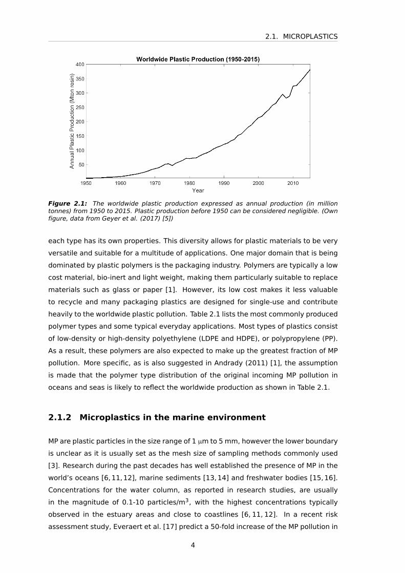
tonnes in 2015 [5] and continues to rise, as shown in Figure 2.1. Densely populated
or industrialised areas logically form the main land-based source of plastic pollution
to the ocean water bodies [6]. Typically cited activities that are sources of MP pol-
lution are plastic bag usage [7], coastal recreation [8], wastewater effluent [9] and
fishery [6].
Plastic material is a typically durable and versatile material and the diversity of avail-
able polymers offers a very large range of applications, from soft LLDPE (linear low-
density polyethylene) foils to PVC (polyvinylchloride) piping. However, as a result of
this durability and since a lot of these polymer products are not collected at their end-
of-life stage, the pollution of plastics is also widespread. In 2016, the United Nations
Environmental Program (UNEP) dedicated a copious report to the presence of plastic
debris and MP in the marine environment, acknowledging the extent of this environ-
mental problem and encouraging initiatives and policy changes in order to take on
this issue. In the end, plastic litter in the ocean is considered a “common concern of
humankind” [10].
Plastic materials are polymers chemically synthesised as a concatenation of a basic
brick molecule, the monomer. There are hundreds of different types of polymers and
2.1. MICROPLASTICS
Figure 2.1: The worldwide plastic production expressed as annual production (in milliontonnes) from 1950 to 2015. Plastic production before 1950 can be considered negligible. (Ownfigure, data from Geyer et al. (2017) [5])
each type has its own properties. This diversity allows for plastic materials to be very
versatile and suitable for a multitude of applications. One major domain that is being
dominated by plastic polymers is the packaging industry. Polymers are typically a low
cost material, bio-inert and light weight, making them particularly suitable to replace
materials such as glass or paper [1]. However, its low cost makes it less valuable
to recycle and many packaging plastics are designed for single-use and contribute
heavily to the worldwide plastic pollution. Table 2.1 lists the most commonly produced
polymer types and some typical everyday applications. Most types of plastics consist
of low-density or high-density polyethylene (LDPE and HDPE), or polypropylene (PP).
As a result, these polymers are also expected to make up the greatest fraction of MP
pollution. More specific, as is also suggested in Andrady (2011) [1], the assumption
is made that the polymer type distribution of the original incoming MP pollution in
oceans and seas is likely to reflect the worldwide production as shown in Table 2.1.
2.1.2 Microplastics in the marine environment
MP are plastic particles in the size range of 1 µm to 5 mm, however the lower boundary
is unclear as it is usually set as the mesh size of sampling methods commonly used
[3]. Research during the past decades has well established the presence of MP in the
world’s oceans [6,11,12], marine sediments [13,14] and freshwater bodies [15,16].
Concentrations for the water column, as reported in research studies, are usually
in the magnitude of 0.1-10 particles/m3, with the highest concentrations typically
observed in the estuary areas and close to coastlines [6, 11, 12]. In a recent risk
assessment study, Everaert et al. [17] predict a 50-fold increase of the MP pollution in
4

CHAPTER 2. LITERATURE REVIEW
Table 2.1:Overview of the most common polymer types, including their densities and annual produc-tion, expressed as percentage of the total worldwide plastics production. PP = polypropylene,LDPE = low-density polyethylene, HDPE = high-density polyethylene, PS = polystyrene, PA =polyamide (nylon), PET = polyethylene therephthalate, PVA = polyvinyl alcohol, CA = cellu-lose amide, PVC = polyvinyl chloride. PA’s annual production was reported as <3%, CA’s andPVA’s was not mentioned but assumed 1.5%, in order to add up to 100% for the sake of futurecalculations. [1]
Polymer Density Range Average Density Annual Applications[g/cm3] [g/cm3] Production [%]
PP [0.89, 0.91] 0.900 24 Bottle caps,netting
LDPE [0.91, 0.94] 0.925 21 Plastic bags,straws
HDPE [0.93, 0.98] 0.955 17 Milk jugsPS [1.04, 1.11] 1.075 6 Food containers,
Foam cupsPA [1.13, 1.15] 1.140 3 Netting, trapsPET [1.19, 1.35] 1.270 7 BottlesPVA [1.19, 1.35] 1.270 1.5 Glue, PlasterCA [1.27, 1.34] 1.305 1.5 Cigarette filtersPVC [1.20, 1.45] 1.325 19 Cups, Bottles,
Plastic Film
terms of mass by 2100, reporting calculations of 9.6 to 48.8 particles/m3, respectively
a best-case and a worst-case scenario. However, most of the datasets cited in these
studies are limited to the larger fraction of MP. However, in Li et al. (2016) [6], for
example, only 2 of 26 included studies report their findings with a size range down
to 50 µm and in a relevant concentration unit (particles/m3). This still excludes an
important fraction of the MP size range, especially when results are expressed based
on number of particles. Studies point to a higher number-based frequency of smaller
particles [18, 19]. In fact, these 2 studies mentioned in Li et al. (2016) [6] report
concentrations of 4 594 and 16 000 particles/m3, respectively [20] and [21], which is
considerably higher when compared to other reported values. This goes to show that
the sampling method plays a crucial role in investigating the extent of the pollution
of MP in oceans and seas.
This research challenge is in line with another assumption, also proposed in Everaert
et al. [17]. It is based on the fact that researchers usually do not include a lower
limit for MP. As mentioned above, the lower limit of the MP size range is typically
set in accordance with the sampling method and has become a loose and arbitrary
border. As an example, in Desforges et al. (2014) [20], a sieve down to 62.5 µm
is used, while in many other on-sea sampling campaigns neuston trawling nets with
pore sizes from 150 µm [19] over 200 µm [18] to 330 µm [22] are used, for example.
Like this, the selection of sampling device or method might automatically exclude
smaller plastic fragments, such as nanoplastics (NP) and even the smaller fraction
5
2.1. MICROPLASTICS
of MP, which represent a much smaller pollution on mass basis but not on number
basis and in terms of ecological threat. However, studies rarely focus on this form
of pollution. Therefore, it can be assumed that measurements and research on MP
underestimate the total pollution by plastics when the sampling method’s lower size
limit excludes a certain fraction of MP.
Typically, two types of MP are defined: primary MP and secondary MP. The first group
consists of MP that are introduced directly into the ocean. On the one hand they are
engineered as micromaterial for application in consumer products, such as cosmet-
ics, paints or cleaning agents [23]. On the other hand, MP are also released directly
by means of ship-breaking or via industrial abrasives [1]. However, it is suggested
that the majority of plastic microfragments in the marine environment are due to
the degradation of plastic litter in the oceans. These are categorised as secondary
MP. Typically, photodegradation is the first degeneration step, usually followed by
thermooxidative degeneration, i.e. slow oxidation of the molecules, and/or biodegra-
dation [1].
The widespread pollution of MP has various consequences on individual organisms
and ecosystems. The threats of MP can be discussed based on three categories: the
particles themselves are a) a physical hazard, b) the particles can act as a vector
for alien species, the biological hazard, and c) the presence of other products (e.g.
plasticizers or coatings) associated with MP particles constitutes a chemical hazard.
a) The physical hazard includes the ingestion of MP particles by individual organ-
isms. An important consequence of this ingestion is weight loss and starvation of
individuals as they stop eating with a permanently filled stomach as the plastic
particles are not broken down by the digestive system of the animal. Other bio-
logical effects are the onset of oxidative stress, the inhibition of photosynthesis in
plankton and the occurrence of inflammatory reactions in tissues [11]. These phe-
nomena have been well documented for e.g. fish [24], benthic species, [25, 26]
sea birds [27,28] and commercial species for human consumption, such as mus-
sels and shrimps [11]. Additionally, organisms that have ingested MP, are also
shown to fragment the particles in their digestive system, leading to an increase
in smaller MP which can be excreted by the organisms. This suggests that higher
animals, such as fish and birds, act as biovectors of MP particles to more remote
oceanic regions [27]. These findings support the studied widespread character of
MP pollution and its impact on ecosystems on a large spatial scale [1].
b) The biological hazard is the consequence of the emergence of MP as a new
solid area on which marine microorganisms can grow. This growth has been char-
acterized in many studies and it is shown that the bacterial community can be
6
CHAPTER 2. LITERATURE REVIEW
very diverse and significantly different from communities as they occur in seawa-
ter [29]. As a result, the plastic particle acts as a freely moving vector of specific
microbial communities which may lead to species dispersal and the introduction
of alien species in ecosystems. Additionally, the biological activity of microor-
ganisms on the polymer surface may lead to a higher leaching rate of additives
present in the plastic particle, contributing to the chemical hazard as well [11].
The concept of biofouling of MP comes forward in many studies on MP and it is an
important characteristic, not only in terms of an ecological opportunity or threat,
but also in terms of the behaviour of the colonised particles themselves [30–33],
which will be discussed later.
c) The chemical hazard associated with MP pollution originates from different classes
of products. First of all, plastics contain various low-molecular additives next to
their main structure of polymer chains [4]. Additives commonly encountered in-
clude phtalates and bisphenol A. These are used as plasticiser (main compound
and auxiliary compound, respectively) in order to make the polymers easier to
process. These additives (up to 50% of the end product [3]) have been shown
to lead to endocrine disruption in organisms as they mimic or disrupt endoge-
nous hormones [11]. Secondly, persistent organic pollutants (POPs) present at
low concentrations in seawater can sorb onto the particle’s surface. The equi-
librium distribution coefficient K for common POPs ranges from 103 to 105 L/kg
towards sorption on plastic particles in a plastic-water system [3]. This leads to
an increase of their concentration by different orders of magnitude [24]. Examples
of such POPs are polycyclic aromatic hydrocarbons (PAHs), chlorinated benzenes
and DDT [11] and they are typically toxic to humans and wildlife in natural con-
centrations [34]. In this way, MP act as a vector of these POPs that spreads them
throughout marine ecosystems. Also, both the plastics’ additives and the con-
centrated POPs can enter an organism after ingestion of an MP particle, forming
an additional toxicological pathway associated with MP pollution [11]. The actual
release of these adsorbed chemical from the plastic particles into the organism’s
tissues has been investigated by thermodynamical modelling [35] and laboratory
tests [36]. Field research on sea birds showed detection of brominated synthetic
compounds that were not found in the birds’ prey, however the same compounds
were found after analysis of the MP present in the birds’ stomachs [28].
2.1.3 Microplastic properties, biofouling and behaviour
There are various properties of MP that define their fate once released into seas and
oceans. Certain particles are bound to stay afloat for a long time, others are assumed
7
2.1. MICROPLASTICS
to reside somewhere in the water column for long and, finally, others will quickly
sink to the bottom and settle as part of the sea floor sediment. The most important
defining properties are the particle’s polymer type, density, rise velocity and size.
The polymer type, by consequence, defines the particle’s original density and its hy-
drophobic attributes, which will play a role in their initial behaviour in the seawater.
The MP’s size is an important parameter that also influences the particle’s buoyancy
in a certain medium as well as the rise velocity. The rise velocity is defined by the
necessary time for a particle to cover a certain vertical distance, which can be pos-
itive (rising particle) or negative (sinking particle). A perfectly spherical particle, for
example, is hindered less by drag forces than an irregularly shaped particle and will,
by consequence, have a higher rise velocity.
The particle size is also related to the degree of biofouling that is possible and the
influence of this biofouling on the final behaviour of a particle. A fundamental paper
on mechanical characteristics of biofilms report a wet density of 1.14 g/cm3 of biofilms
[37], which is higher than seawater density. The average diameter of a bacterial cell
is reported to be in the magnitude of µm, so an MP particle of 10 µm will be affected
more by the attachment of a bacterial cell of a certain density than a particle of 5
mm [38]. As mentioned above, the plastic surface is an interesting surface on which
microorganisms are likely to attach. Zettler et al. (2013) [29] describe their findings
on colonisation of microorganisms on plastic debris collected from the top layer of
open sea, coining these ecosystems the "Plastisphere". The identified organisms were
very specific and the colonisation revealed significant differences with respect to what
is found in the seawater surrounding the plastic particles. In their analyses, surface
coverage by biomass amounted up to 8%.
As a result of the above factors, the vertical behaviour of MP in ocean waters can vary
strongly and it cannot be simplified to a floating fraction of a density lower relative
to the density of seawater and a settling fraction of higher density. In Law et al.
(2010) [39], the authors report their findings on one of the notorious plastic gyres. A
relatively constant amount of floating MP of particularly low density (mainly PP, LDPE
and HDPE) is described over the years, even though, as can be seen in Figure 2.1,
plastic production grows yearly. Therefore, it was already assumed that these lighter
plastic fragments eventually sink below the surface as well. At the same time, studies
indicate that most plastic particles found in sea sediments are of higher density than
seawater [40]. This has led to the largely unanswered hypothesis of ’lost’ plastics
throughout the vertical water column. In previous studies, the vertical behaviour
of MP particles has already been studied and linked to various properties. Reisser
et al. (2015) [19] describe the faster vertical mixing of smaller floating particles
compared to bigger particles, leading to an observed larger vertical decay of the
8
CHAPTER 2. LITERATURE REVIEW
presence of MP based on mass rather than on number. Also, Kooi et al. (2017)
[38] constructed a model to study the vertical distribution in the water column and
the effect of biofouling on this behaviour. Positively buoyant particles exposed to
marine biofouling conditions, such as light and oxygen, are prone to develop a biofilm
aggregate on their surface, changing its properties as a whole. This is assumed to
lead to a higher density in such a way that the particles might start sinking down.
However, defouling due to grazing and light deficiency [41] supposedly leads to a
vertical oscillatory pattern and a long residence time throughout the water column
[38].
2.2 Seawater Desalination
2.2.1 Desalination
The depletion of water and drinking water resources is a major environmental chal-
lenge. Various regions are already faced with an increased drought and the demand
for drinking water grows. One option to access a source of drinking water is the de-
salination of seawater. On average, seawater contains about 35 grams of salt per
litre and it can be as high as 40 g/L [42, 43]. In order to produce drinking water,
these salts need to removed together with other contaminants such as organic mat-
ter, microorganisms and particulate matter. There are two main technologies for
desalination; thermal and membrane-based. Among these, various technologies are
available. Examples for thermal desalination are multi-stage flash (MSF) and multi-
effect flash (MED), membrane-based techniques are for example electrodialysis (ED)
and reverse osmosis (RO). Over the last three decades, crucial improvements in RO
technology have launched RO membranes as the go-to option for new desalination
installations, meaning membrane-based desalination has taken over thermal desali-
nation [44]. Only in the Middle East thermal desalination is still prominently present
given the low cost of fossil fuels and the bad quality of seawater, hampering the ap-
plicability of membranes. Currently, the total desalination capacity reaches 90 million
m3/d [45]. As can be seen in Figure 2.2, RO comprises more than half of the de-
salination plants worldwide [46]. Despite its high energy demand, this is a growing
technology and RO plants are surging. Especially in areas close to sea, close to a high
energy supply and with little access to other drinking water sources, RO is technology
gaining popularity.
Naturally, during desalination processes, large fluxes of seawater are taken up and
pass through the system in order to separate particles and dissolved molecules from
the seawater stream. A pure water stream is the end product of the entire process.
9

2.2. SEAWATER DESALINATION
Figure 2.2: An overview of the worldwide distribution of desalination technologies. RO =Reverse Osmosis; MSF = Multi-Stage Flash; MED = Multi-Effect Distillation; ED = Electrodialysis;EDR = Electrodialysis Reversal; EDL = Electric Double Layer; NF/SR = Nanofiltration/SulphateRemoval. (Own figure, data from GWI (2012) [45])
However, there are also some waste streams (rejects) created throughout the sys-
tem, which are typically being sent back to the source (e.g. sea or ocean), with post
treatment if necessary. In this way, a potential flux of plastic particles passes through
such desalination systems as well, which offers an opportunity for the removal of MP
from seawater. Before focussing on this opportunity, the typical layout of seawater
reverse osmosis (SWRO) plants is described which will play a central role in this study.
2.2.2 Reverse Osmosis
RO is a membrane technology where a water stream under high pressure (up to 60
bars [47]) is forced through a semi-permeable membrane: the water is able to pass
through the filter while particulates and dissolved salts are rejected with a rejection of
up to 99% [48]. The efficiency of RO is typically around 50 %. This means that half of
the incoming water is purified while the other half of the stream is a reject stream con-
taining the removed particles and salt molecules. The cut-off size of the RO modules
is very small (less than 1 nm [46]) resulting in a high sensitivity to fouling, leading
to an inoperable system due to too high pressure drops, or even irreversible fouling
due to the presence of suspended solids [46]. Therefore, the seawater sent to the
RO membrane modules requires pretreatment steps to allow a favourable operation.
10
CHAPTER 2. LITERATURE REVIEW
Typical pretreatment can consist of screening, coagulation-flocculation, multi-media
filtration [43], activated carbon modules, microfiltration (MF), etc. [46].
2.2.3 RO Pretreatment
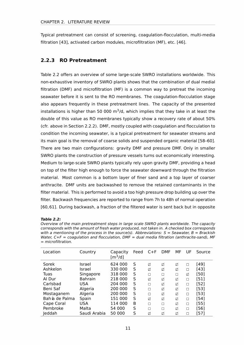
Table 2.2 offers an overview of some large-scale SWRO installations worldwide. This
non-exhaustive inventory of SWRO plants shows that the combination of dual medial
filtration (DMF) and microfiltration (MF) is a common way to pretreat the incoming
seawater before it is sent to the RO membranes. The coagulation-flocculation stage
also appears frequently in these pretreatment lines. The capacity of the presented
installations is higher than 50 000 m3/d, which implies that they take in at least the
double of this value as RO membranes typically show a recovery rate of about 50%
(cfr. above in Section 2.2.2). DMF, mostly coupled with coagulation and flocculation to
condition the incoming seawater, is a typical pretreatment for seawater streams and
its main goal is the removal of coarse solids and suspended organic material [58–60].
There are two main configurations: gravity DMF and pressure DMF. Only in smaller
SWRO plants the construction of pressure vessels turns out economically interesting.
Medium to large-scale SWRO plants typically rely upon gravity DMF, providing a head
on top of the filter high enough to force the seawater downward through the filtration
material. Most common is a bottom layer of finer sand and a top layer of coarser
anthracite. DMF units are backwashed to remove the retained contaminants in the
filter material. This is performed to avoid a too high pressure drop building up over the
filter. Backwash frequencies are reported to range from 7h to 48h of normal operation
[60,61]. During backwash, a fraction of the filtered water is sent back but in opposite
Table 2.2:Overview of the main pretreatment steps in large scale SWRO plants worldwide. The capacitycorresponds with the amount of fresh water produced, not taken in. A checked box correspondswith a mentioning of the process in the source(s). Abbreviations: S = Seawater, B = BrackishWater, C+F = coagulation and flocculation, DMF = dual media filtration (anthracite-sand), MF= microfiltration.
Location Country Capacity Feed C+F DMF MF UF Source[m3/d]
Sorek Israel 624 000 S 2� 2� 2� 2 [49]Ashkelon Israel 330 000 S 2� 2� 2� 2 [43]Tuas Singapore 318 000 S 2 2 2 2� [50]Al Dur Bahrain 218 000 S 2� 2� 2� 2 [51]Carlsbad USA 204 000 S 2 2� 2� 2 [52]Beni Saf Algeria 200 000 S 2 2� 2� 2 [53]Mostaganem Algeria 200 000 S 2 2� 2� 2 [53]Bahía de Palma Spain 151 000 S 2� 2� 2� 2 [54]Cape Coral USA 114 000 B 2 2 2� 2 [55]Pembroke Malta 54 000 S 2 2 2� 2 [56]Jeddah Saudi Arabia 50 000 S 2� 2� 2� 2 [57]
11
2.2. SEAWATER DESALINATION
direction (bottom-to-top). The backwash volume ranges typically from 2% to 5%,
leading to a recovery of 95-98% for DMF [60]. The (micro)filtration step afterwards
is to further remove the fine fraction of suspended solids and organic matter before
sending the water to the RO membrane units [58–61]. The reported pore sizes for MF
in the SWRO plants in Table 2.2 range from 1 to 10 µm.
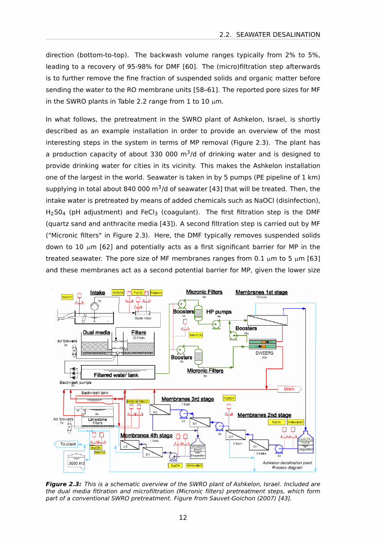
In what follows, the pretreatment in the SWRO plant of Ashkelon, Israel, is shortly
described as an example installation in order to provide an overview of the most
interesting steps in the system in terms of MP removal (Figure 2.3). The plant has
a production capacity of about 330 000 m3/d of drinking water and is designed to
provide drinking water for cities in its vicinity. This makes the Ashkelon installation
one of the largest in the world. Seawater is taken in by 5 pumps (PE pipeline of 1 km)
supplying in total about 840 000 m3/d of seawater [43] that will be treated. Then, the
intake water is pretreated by means of added chemicals such as NaOCl (disinfection),
H2S04 (pH adjustment) and FeCl3 (coagulant). The first filtration step is the DMF
(quartz sand and anthracite media [43]). A second filtration step is carried out by MF
("Micronic filters" in Figure 2.3). Here, the DMF typically removes suspended solids
down to 10 µm [62] and potentially acts as a first significant barrier for MP in the
treated seawater. The pore size of MF membranes ranges from 0.1 µm to 5 µm [63]
and these membranes act as a second potential barrier for MP, given the lower size
Figure 2.3: This is a schematic overview of the SWRO plant of Ashkelon, Israel. Included arethe dual media fitlration and microfiltration (Micronic filters) pretreatment steps, which formpart of a conventional SWRO pretreatment. Figure from Sauvet-Goichon (2007) [43].
12
CHAPTER 2. LITERATURE REVIEW
limit of MP of 1 µm. Therefore, it is hypothesised that the majority of MP present in
seawater are held up at least at the MF step in the pretreatment process of RO and,
as a result, does not end up at the RO membranes themselves as the MP particles are
by definition too big.
Previous studies that follow up the fate of MP in wastewater treatment plants (WWTP)
already pointed in the direction of these unit processes as being most effective to
retain MP. These studies [64–68] sample at different locations in the plant and quantify
the removal of MP over every step. In Michielssen et al. (2016) for example, 3 WWTP
are sampled with different treatment steps. In the end, the removal efficiency of each
sampled step is reported and among the highest removal rates were a granular sand
filter step and an (MF) membrane process (pore size 0.2 µm), respectively 72.1% and
99.1% [64]. In another recent study on the fate of MP in WWTP systems, a bench-
scale gravity filter (anthracite-sand-gravel), typical as tertiary treatment in WWTP, is
constructed to evaluate the removal of spiked MP in a WWTP slurry stream (5 mg
MP/L). The authors report no breakthrough and a retrieval of more than 95% of the
spiked MP in the backwash (water and air sparging, 15 min) after pouring 2L of spiked
influent [68].
2.2.4 Other aspects of SWRO
Two other relevant aspects of an RO installation are the intake depth and the produc-
tion of brine. The intake system is a key component of the process as it determines
the feed water quality and the performance of the treatment steps down the line.
The current method of choice is open ocean intake [69], as it requires lower pumping
power but may lead to fairly highly contaminated water in terms of turbidity and sus-
pended debris [70], which may include MP particles of a relatively low density. The
intake depth for open water intake usually ranges from 1 to 6 m [70], with 4 m being
an often encountered value [69,71,72]. Another option is deep intake, with pumping
depths down to 35 m where the debris load is lower [69, 70]. However, this is less
feasible to construct and operate and it is not used widely.
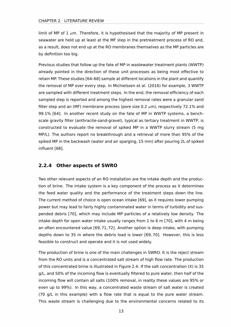
The production of brine is one of the main challenges in SWRO. It is the reject stream
from the RO units and is a concentrated salt stream of high flow rate. The production
of this concentrated brine is illustrated in Figure 2.4. If the salt concentration (X) is 35
g/L, and 50% of the incoming flow is eventually filtered to pure water, then half of the
incoming flow will contain all salts (100% removal, in reality these values are 95% or
even up to 99%). In this way, a concentrated waste stream of salt water is created
(70 g/L in this example) with a flow rate that is equal to the pure water stream.
This waste stream is challenging due to the environmental concerns related to its
13
2.2. SEAWATER DESALINATION
Figure 2.4: This graphic presents a simplified diagram of 1 RO unit where X is the salt con-centration in g/L. A recovery of 50% and a salt removal efficiency of 100% is assumed. Thisresults in a concentrated waste stream of salt water (brine) with a flow rate equal to the purewater stream, i.e. half of the incoming feed to the RO unit.
disposal in the marine environment, e.g. local brine plumes of high concentration,
affecting the surrounding ecosystem. Reduced dissolved oxygen concentration, the
disruption of the salt excretion system of fish and the disruption of larval development
are documented ecological impacts [73]. Other concerns are the higher temperature
of the brine stream and its increased alkalinity [73]. However, direct discharge back
into the sea is one of the current methods to handle this waste stream with a high
salt content [48]. Therefore, as it is a main environmental challenge, multiple efforts
haven been taken to tackle this problem instead of direct discharge. Examples of
such solutions are dilution [74] or salt recovery from the waste stream [75].
These two aspects (intake depth and brine waste) are important parameters when
considering the potential removal of MP from seawater that is treated in SWRO facil-
ities. The intake depth might influence the amount and the types of polymer taken
in by the system, corresponding with the vertical distribution of MP in the water.
The brine is a challenge in SWRO operation and its increased salt content (and its
increased density as a result) might prove a possible resource when looking into sep-
aration of MP from pretreatment filtrates by ways of density differences.
14

CHAPTER 2. LITERATURE REVIEW
2.3 Research Gaps
In the following research, the main goal is to look into the possibility of removing MP
particles taken in by SWRO installations. However, there are still many gaps in the
literature about the behaviour of the MP. First of all there is the occurrence issue. By
now there have been various sampling studies to identify and quantify the presence
of MP pollution in the oceans and seas. Yet, there are limits to these findings such
as the lower size limit of sampled particles or the depth at which samples are taken.
Up to now, the smallest fraction of MP (< 50 µm) is barely included in measurements
and there is little known on the occurrence and distribution of the MP deeper in the
water column, the so-called ’lost’ plastics (Section 2.1.2). These issues give rise to
the incomplete image there is concerning the marine MP pollution.
Secondly, how do MP behave in the natural environment of ocean and seas? Wind,
waves and currents are forces that act on the particles while degradation and bio-
fouling influence their characteristics, such as shape, size and density (Section 2.1.3).
These factors influence the vertical distribution and at the same time the fraction that
might be taken in by SWRO pumps.
Thirdly, how do MP behave throughout the process of SWRO? The MP present in the
seawater taken in by SWRO plants pass the same process steps as the water. For this
reason, it will be interesting to investigate their behaviour and the removal efficiency
of these various steps in order to point out where the hotspots of MP occur within the
process. Earlier studies already point to the strong removal capacity of unit processes
such as gravity filters and MF membranes in terms of MP in WWTP. However, the
previous bench-scale study on DMF focussed on WWTP streams and only filtered a
2L spike, not allowing a longer operation with a more continuous spike which may
influence the result of MP retrieval in the backwash stream [68]. If the long-term
operation and MP removal of this step in the context of SWRO is further investigated,
this will allow to act more effectively in terms of the removal of MP from the reject
streams created in DMF and MF before these streams would end up back into the
seawater, including the MP particles. In the following chapter, the main research
questions of this thesis are formulated to answer some of these research issues.
15

2.3. RESEARCH GAPS
16
CHAPTER 3
RESEARCH OUTLINE
3.1 Research Questions
MP pollution is a growing threat for marine ecosystems and as a pollutant, the parti-
cles act as a hazard in multiple ways. It is clear from the above that research concern-
ing this MP pollution is very hard to characterise and to generalise. There are many
factors to be taken into account: vicinity of pollution sources (e.g. industry, cities or
fishery), ocean currents, wind conditions, polymer type and density, rate of biofouling,
etc. Therefore, it is hard to quantify the presence of these MP particles in the seawa-
ter. However, their presence has been evidenced and their impact as well. Therefore,
this research will focus on a method to remove a fraction of the MP present in seawa-
ter relatively close to coastal areas, where concentrations are typically higher than in
open water (2.1.2). SWRO installations draw in big flows of seawater to produce e.g.
drinking water. This implies that the MP contained in this seawater also pass through
the system and, as it they are not known to be removed or processed, end up in the
sea again as part of the pretreatment reject streams.
In this view, this research will firstly focus on the behaviour of MP in seawater and
how biofouling phenomena influence its density. This will give an indication of the
behaviour of MP in the vertical water column, rather than only at the surface of the
water. It is assumed that, due to biofouling, the less dense polymers (PP and PE) will
sink, but much slower than for example PVC or PET particles. The aim of this set-up
is to evidence the probability of taking in predominantly PE and PP particles when
pumping at rather shallow depths, as happens in SWRO installations 2.2.4.
Secondly, as can be seen in Table 2.2, many large-scale SWRO plants incorporate
both DMF and MF as a pretreatment of the incoming water before it is sent over
the RO membranes. Therefore, there will be an attempt to describe the behaviour
of MP throughout these pretreatment steps common in SWRO installations and how
efficiently this pretreatment functions in terms of MP removal. Also, the quantifica-
tion of the MP contained in the resulting streams poses a big challenge and the way
3.2. EXPERIMENTAL RESEARCH
these problems are answered during the analysis of the results will also feature as an
important aspect of this research study.
Finally there will be an attempt to construct a mass balance to estimate the flux and
distribution of MP particles present in the seawater treated in SWRO installations.
This allows to create a more specific image of the presence and fate of MP in these
installations and to discuss their potential for removal from the process streams.
3.2 Experimental Research
In order to answer these research questions, both predictive calculations as well as
experimental research will be conducted. The experimental part of this research is
mainly designed to study the behaviour and fate of MP particles in SWRO installations.
On the one hand, more information about the effect of biofouling on the floating
behaviour of plastics in seawater is relevant to better predict what kind and how
many MP enter an SWRO treatment process. On the other hand, removal efficiencies
of MP in the different subprocesses within the SWRO system are necessary to describe
the flux of MP and to make predictions concerning removal and recovery potential of
(micro)plastics.
As described in 2.1.3, earlier experimental work supports the hypothesis that bio-
fouling influences the density and floating behaviour of MP. To further comprehend
this phenomenon a first experimental set-up is designed to study the influence of bio-
fouling on the density of plastic particles. More specific, the goal of the experiment is
to quantify the increase of density in relation to the amount of biomass present on a
certain particle.
Later on, a bench-scale simulation of SWRO pretreatment processes is constructed
and evaluated in terms of MP removal. The goal of the experiments is to predict where
the MP will end up during the passage through a series of pretreatment steps for RO.
Finally, on the one hand, an estimate of the plastic flux throughout large-scale SWRO
installations will be performed based on data retrieved from literature. On the other
hand, based on the experimental results from the bench-scale pretreatment simula-
tions, a mass balance over both unit processes (i.e. DMF and MF) will be constructed
to further elaborate on the flux of MP in SWRO installations and on their potential for
removal.
18
CHAPTER 4
MATERIALS AND METHODS
4.1 Biofouling
4.1.1 Tank Set-up
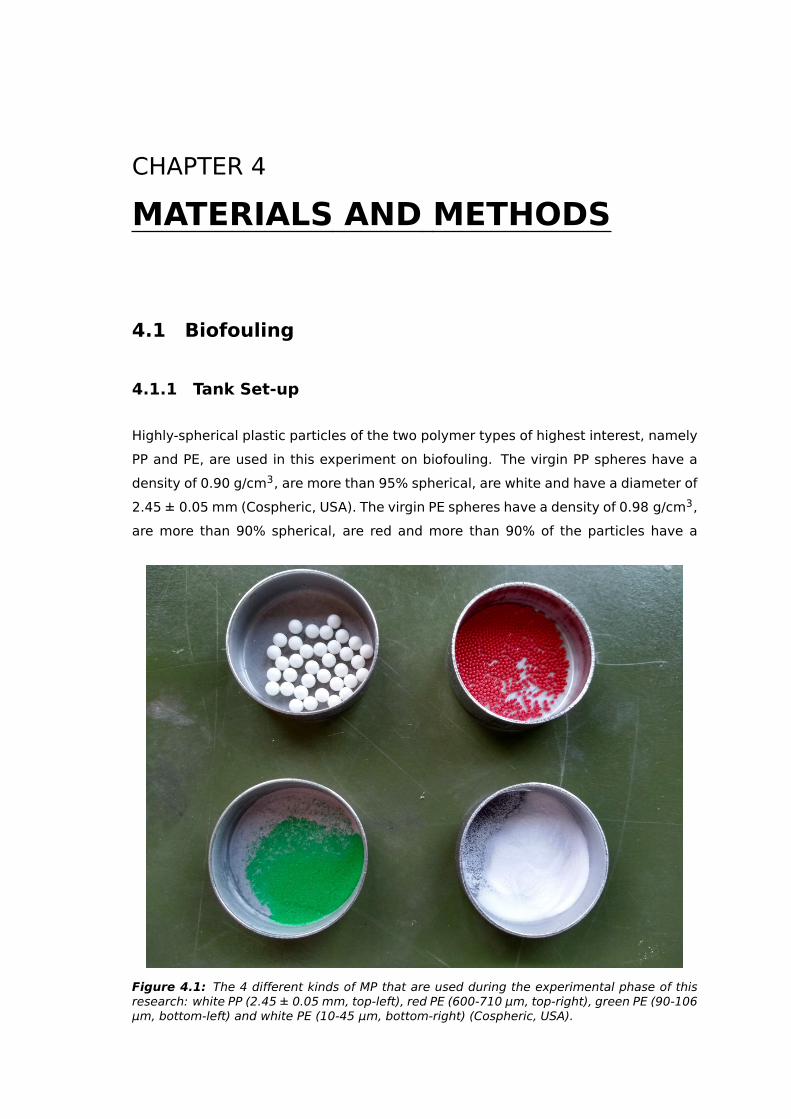
Highly-spherical plastic particles of the two polymer types of highest interest, namely
PP and PE, are used in this experiment on biofouling. The virgin PP spheres have a
density of 0.90 g/cm3, are more than 95% spherical, are white and have a diameter of
2.45 ± 0.05 mm (Cospheric, USA). The virgin PE spheres have a density of 0.98 g/cm3,
are more than 90% spherical, are red and more than 90% of the particles have a
Figure 4.1: The 4 different kinds of MP that are used during the experimental phase of thisresearch: white PP (2.45 ± 0.05 mm, top-left), red PE (600-710 μm, top-right), green PE (90-106μm, bottom-left) and white PE (10-45 μm, bottom-right) (Cospheric, USA).
4.1. BIOFOULING
diameter between 600 µm and 710 µm (Cospheric, USA). As the shape and size of the
polymer spheres are very uniform, the variation in density can be attributed to the
amount of biofouling that occurred during the experiment.
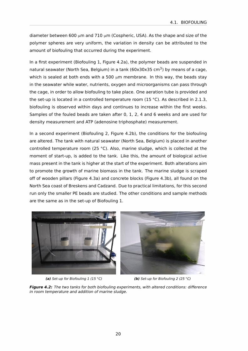
In a first experiment (Biofouling 1, Figure 4.2a), the polymer beads are suspended in
natural seawater (North Sea, Belgium) in a tank (60x30x35 cm3) by means of a cage,
which is sealed at both ends with a 500 µm membrane. In this way, the beads stay
in the seawater while water, nutrients, oxygen and microorganisms can pass through
the cage, in order to allow biofouling to take place. One aeration tube is provided and
the set-up is located in a controlled temperature room (15 ◦C). As described in 2.1.3,
biofouling is observed within days and continues to increase within the first weeks.
Samples of the fouled beads are taken after 0, 1, 2, 4 and 6 weeks and are used for
density measurement and ATP (adenosine triphosphate) measurement.
In a second experiment (Biofouling 2, Figure 4.2b), the conditions for the biofouling
are altered. The tank with natural seawater (North Sea, Belgium) is placed in another
controlled temperature room (25 ◦C). Also, marine sludge, which is collected at the
moment of start-up, is added to the tank. Like this, the amount of biological active
mass present in the tank is higher at the start of the experiment. Both alterations aim
to promote the growth of marine biomass in the tank. The marine sludge is scraped
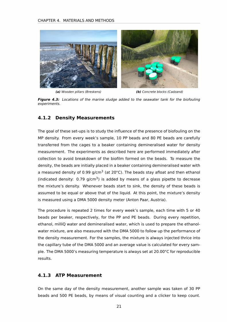
off of wooden pillars (Figure 4.3a) and concrete blocks (Figure 4.3b), all found on the
North Sea coast of Breskens and Cadzand. Due to practical limitations, for this second
run only the smaller PE beads are studied. The other conditions and sample methods
are the same as in the set-up of Biofouling 1.
(a) Set-up for Biofouling 1 (15 ◦C) (b) Set-up for Biofouling 2 (25 ◦C)
Figure 4.2: The two tanks for both biofouling experiments, with altered conditions: differencein room temperature and addition of marine sludge.
20
CHAPTER 4. MATERIALS AND METHODS
(a) Wooden pillars (Breskens) (b) Concrete blocks (Cadzand)
Figure 4.3: Locations of the marine sludge added to the seawater tank for the biofoulingexperiments.
4.1.2 Density Measurements
The goal of these set-ups is to study the influence of the presence of biofouling on the
MP density. From every week’s sample, 10 PP beads and 80 PE beads are carefully
transferred from the cages to a beaker containing demineralised water for density
measurement. The experiments as described here are performed immediately after
collection to avoid breakdown of the biofilm formed on the beads. To measure the
density, the beads are initially placed in a beaker containing demineralised water with
a measured density of 0.99 g/cm3 (at 20◦C). The beads stay afloat and then ethanol
(indicated density: 0.79 g/cm3) is added by means of a glass pipette to decrease
the mixture’s density. Whenever beads start to sink, the density of these beads is
assumed to be equal or above that of the liquid. At this point, the mixture’s density
is measured using a DMA 5000 density meter (Anton Paar, Austria).
The procedure is repeated 2 times for every week’s sample, each time with 5 or 40
beads per beaker, respectively, for the PP and PE beads. During every repetition,
ethanol, milliQ water and demineralised water, which is used to prepare the ethanol-
water mixture, are also measured with the DMA 5000 to follow up the performance of
the density measurement. For the samples, the mixture is always injected thrice into
the capillary tube of the DMA 5000 and an average value is calculated for every sam-
ple. The DMA 5000’s measuring temperature is always set at 20.00◦C for reproducible
results.
4.1.3 ATP Measurement
On the same day of the density measurement, another sample was taken of 30 PP
beads and 500 PE beads, by means of visual counting and a clicker to keep count.
21
4.2. SWRO PRETREATMENT SIMULATION
The beads are then carefully placed in a beaker of 10 mL of milliQ water. A sonication
procedure (15 minutes at 30 ◦C) is performed to remove all biomass present on the
beads and transfer it to the water phase. These conditions are selected to be long
enough to allow the removal of biofilm from the plastic particles, while keeping the
temperature at the lower limit of the machine to minimise a temperature shock effect
for the microorganisms. This water phase is then analysed for ATP concentration with
a luminescence measurement using an Infinite 200 PRO Series Multimode Reader
apparatus (Tecan Trading AG, USA). After addition of BacTiter-GloTM (Promega, USA),
the luminescence intensity is measured which is related to the ATP concentration in
the samples. The relation between the signal and the ATP concentration is followed up
by adding a dilution series from a reference sample of ATP in a 96-well tray (Greiner
Flat Black, Greiner, Austria). During the Biofouling 1 experiment, the tray is filled with
2x30 volumes of 100 µL from the sonicated samples of either PE or PP (total of 60).
During the Biofouling 2 experiment, as there were only PE beads, the tray is filled with
1x60 volumes of 100 µL from the sonicated sample of PE beads.
4.2 SWRO Pretreatment Simulation
4.2.1 Dual Media Filtration
The main set-up during this research is the dual media filter (DMF) that consists of
anthracite and sand. As mentioned above (Table 2.2), this type of DMF is very com-
mon as a pretreatment step in the larger SWRO plants. The bench-scale filter was
constructed using a hard PVC pipe (1 meter in length and an internal diameter of 34
mm) which is sealed at both ends using a wire gauze of mesh size 60 to keep the filter
material in place during running and during backwash operation. The mesh retains
the sand and anthracite particles but is large enough for the studied MP material and
water to pass freely. In this way, the gauze does not add to the filtering effect of the
DMF itself. The coarse upper layer of the DMF consists of anthracite (size range: 1 to
2 mm), the finer lower layer consists of sand (size range: 0.250 to 1 mm). Before the
implementation, both materials are dried in an oven overnight at 50 ◦C and sieved in
different fractions from which the preferred size fraction is retained. After filling the
column with the filter material, it is first conditioned during two days with unspiked
water to rinse the remaining smaller sand and anthracite particles (< 250 µm) out of
the column in order to ensure a clean operation and to avoid fast clogging of the filter
papers on which the MP are eventually collected. After this procedure, the column is
ready to operate and treat samples of tap water and seawater spiked with MP.
22
CHAPTER 4. MATERIALS AND METHODS
During this experiment, the column is in operation for a total of 4 weeks. In a first
phase, tap water is used as the matrix to evaluate the performance of the column in
terms of removal op MP. The samples are prepared in the following way: 30.0 mg
of green PE beads (90-106 µm, Cospheric, USA) are weighed and treated with a
0.1 %(v/v) Tween 80 solution. Tween has an emulsifying effect and reduces the hy-
drophobicity of the virgin beads, as recommended by the producer. Then, the 30 mg
green PE is added to 10L bottles of water. The exact amount of spiked PE in terms of
number of particle is of course unknown in this way, which is countered by executing
and analysing empty column runs as described below. In a second phase, seawater is
used, spiked with the same MP particles as in the first phase, but in a concentration
that tends to approximate more realistic values. In this case, 3 mg of PE beads is
added to the 10L bottles of seawater. In the second phase (with seawater), smaller
white PE beads (diameter: 10-45 µm, (Cospheric, USA)) are also added at 3 mg per
10L bottle in addition to the 3 mg per 10L of green PE beads (diameter: 90-106 µm).
The influent feed is constantly stirred by a magnetic stirrer on the bottom of the bot-
tle to homogenise the MP concentration in the feed while it is being pumped over
the filter column. All connections for water flows are constructed using Festo (Ger-
many) norprene tubes and fittings. A Masterflex L/S-Economic Drive pump 115 VAC
(Cole-Parmer, USA) is installed which was used for both normal (top-to-bottom) and
backwash (bottom-to-top) operation. Switching between both regimes is possible by
swapping the tubes of the installation. The pump is able to operate between 0.072
and 174 L/h and it is calibrated before each filtration period at 9 L/h for normal oper-
ation. This corresponds with a loading of 10 m3/m2/h on the used column which is a
typical value for DMF. For backwash, the pump is set to a flow of about 36 L/h [61].
This way, the backwash is performed with a flow rate 4 times higher than the normal
operation, flushing the column with 6L of fresh water during 10 minutes. This leads to
a recovery of 94% (6L of the total of 100L filtered water is used again for backwash)
for this bench-scale system. During backwash, the filter material is allowed to fully
expand, taking up almost the entire volume of the column (1m height) while the built
up contaminants, including the spiked MP, are loosened from the anthracite and sand
and are flushed out by the upstream water flow. After backwash, the filter material
settles gradually with the heavier sand settling at the bottom again. The lighter an-
thracite settles on top of the sand, allowing a new run of normal operation. More
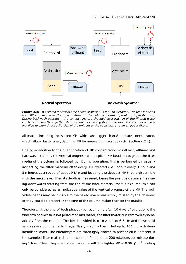
design parameters are listed in Table 4.1. Figure 4.4 provides a sketch of the DMF
set-up.
Both effluent and backwash water are collected for analysis on MP content. The result-
ing streams are immediately passed over a round white Grade 2 filter paper (What-
man, USA) for collection. The filter paper’s maximum pore size is 8 µm. In this way,
23
4.2. SWRO PRETREATMENT SIMULATION
Figure 4.4: This sketch represents the bench-scale set-up for DMF filtration. The feed is spikedwith MP and sent over the filter material in the column (normal operation, top-to-bottom).During backwash operation, the connections are changed so a fraction of the filtered watercan be sent back through the filter material for cleaning (bottom-to-top). The vacuum pump isinstalled to allow direct collection of the effluent or the backwash stream on paper filters.
all matter including the spiked MP (which are bigger than 8 µm) are concentrated,
which allows faster analysis of the MP by means of microscopy (cfr. Section 4.2.4).
Finally, in addition to the quantification of MP concentration of influent, effluent and
backwash streams, the vertical progress of the spiked MP beads throughout the filter
media of the column is followed up. During operation, this is performed by visually
inspecting the filter material after every 10L treated (i.e. about every 1 hour and
5 minutes at a speed of about 9 L/h) and locating the deepest MP that is discernible
with the naked eye. Then its depth is measured, being the positive distance measur-
ing downwards starting from the top of the filter material itself. Of course, this can
only be considered as an indicative value of the vertical progress of the MP. The indi-
vidual beads may be invisible to the naked eye or are simply missed by the observer
or they could be present in the core of the column rather than on the outside.
Therefore, at the end of both phases (i.e. each time after 10 days of operation), the
final fifth backwash is not performed and rather, the filter material is removed system-
atically from the column. The bed is divided into 10 zones of 6.7 cm and these solid
samples are put in an erlenmeyer flask, which is then filled up to 400 mL with dem-
ineralised water. The erlenmeyers are thoroughly shaken to release all MP present in
the sampled filter material (anthracite and/or sand) at 200 rotations per minute dur-
ing 1 hour. Then, they are allowed to settle with the lighter MP of 0.98 g/cm3 floating
24
CHAPTER 4. MATERIALS AND METHODS
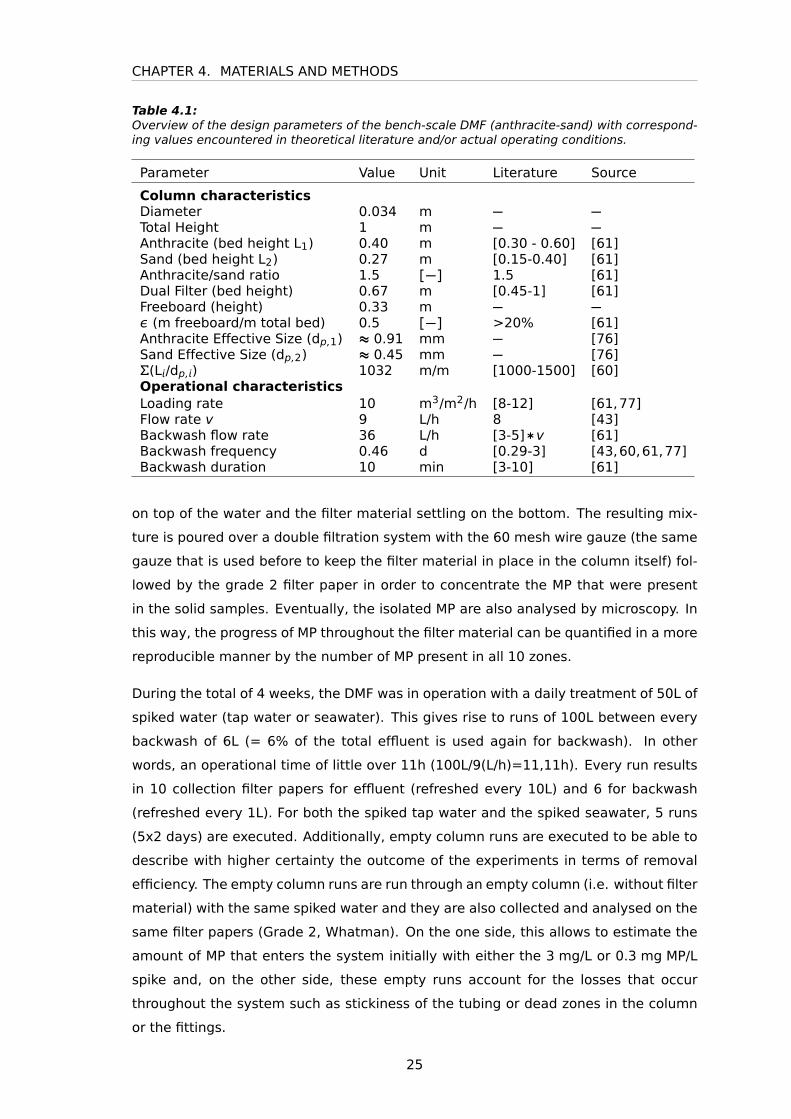
Table 4.1:Overview of the design parameters of the bench-scale DMF (anthracite-sand) with correspond-ing values encountered in theoretical literature and/or actual operating conditions.
Parameter Value Unit Literature Source
Column characteristicsDiameter 0.034 m − −Total Height 1 m − −Anthracite (bed height L1) 0.40 m [0.30 - 0.60] [61]Sand (bed height L2) 0.27 m [0.15-0.40] [61]Anthracite/sand ratio 1.5 [−] 1.5 [61]Dual Filter (bed height) 0.67 m [0.45-1] [61]Freeboard (height) 0.33 m − −ε (m freeboard/m total bed) 0.5 [−] >20% [61]Anthracite Effective Size (dp,1) ≈ 0.91 mm − [76]Sand Effective Size (dp,2) ≈ 0.45 mm − [76](L/dp,) 1032 m/m [1000-1500] [60]Operational characteristicsLoading rate 10 m3/m2/h [8-12] [61,77]Flow rate v 9 L/h 8 [43]Backwash flow rate 36 L/h [3-5]∗v [61]Backwash frequency 0.46 d [0.29-3] [43,60,61,77]Backwash duration 10 min [3-10] [61]
on top of the water and the filter material settling on the bottom. The resulting mix-
ture is poured over a double filtration system with the 60 mesh wire gauze (the same
gauze that is used before to keep the filter material in place in the column itself) fol-
lowed by the grade 2 filter paper in order to concentrate the MP that were present
in the solid samples. Eventually, the isolated MP are also analysed by microscopy. In
this way, the progress of MP throughout the filter material can be quantified in a more
reproducible manner by the number of MP present in all 10 zones.
During the total of 4 weeks, the DMF was in operation with a daily treatment of 50L of
spiked water (tap water or seawater). This gives rise to runs of 100L between every
backwash of 6L (= 6% of the total effluent is used again for backwash). In other
words, an operational time of little over 11h (100L/9(L/h)=11,11h). Every run results
in 10 collection filter papers for effluent (refreshed every 10L) and 6 for backwash
(refreshed every 1L). For both the spiked tap water and the spiked seawater, 5 runs
(5x2 days) are executed. Additionally, empty column runs are executed to be able to
describe with higher certainty the outcome of the experiments in terms of removal
efficiency. The empty column runs are run through an empty column (i.e. without filter
material) with the same spiked water and they are also collected and analysed on the
same filter papers (Grade 2, Whatman). On the one side, this allows to estimate the
amount of MP that enters the system initially with either the 3 mg/L or 0.3 mg MP/L
spike and, on the other side, these empty runs account for the losses that occur
throughout the system such as stickiness of the tubing or dead zones in the column
or the fittings.
25
4.2. SWRO PRETREATMENT SIMULATION
In the second phase of this DMF set-up (all the runs with seawater in Table 4.3), it was
mentioned that smaller PE beads (white, 10-45 µm, bottom-right on Figure 4.1) are
also added as a spike to the influent water. In the first place, it was intended to check
whether it was possible to follow their vertical progress qualitatively through the filter
material, just like was done for the green beads. However, it turned out impossible
to visually discern any of these beads in the column. For that reason, it was chosen
to pass a small fraction of the total volume (2x1L of every run’s 100) over black filter
paper (Grade 918, 90mm diameter, Camlab Ltd) instead for a qualitative study of the
possible breakthrough of these smaller beads in the effluent of the DMF column. This
is an interesting addition to the experimental set-up as these MP represent the lower
limit of the MP size range, which are of major importance in research on MP in general.
4.2.2 Microfiltration
Using a similar set-up as for the DMF experiment, this study was also performed for
the microfiltration (MF) pretreatment step which usually follows the DMF step in the
SWRO pretreatment process (Table 2.2). Given the available PE MP to spike influent
samples (90-106 µm), an MF cartridge of 25 µm (Van Marcke Pro Purifo, Belgium)
was installed. This MF cartridge has a height of 315 mm and a diameter of 135
mm, resulting in a filter surface area of 0.134 m2. The filter works according to
the outside-in principle: water surrounds the outside of the MF filter and is forced
inwards, from where the water can leave the filter cartridge at the top. In practice,
MF membranes are also backwashed frequently to ensure proper operation and to
counter the transmembrane pressure that builds up due to fouling of the membranes.
This backwash is also simulated during the experiment in order to follow up the fate of
the MP, similar to the DMF experiments. For every experiment, there is also an empty
run during which the MF cartridge is uncoupled and 1 run of 6x10L with spiked influent
is passed through the system. Again, the reason for this empty run is to counter the
loss of MP in the tubings, fittings and cartridge holder and to be able to quantify more
accurately the amount of MP that actually passes the system and to construct a total
MP mass balance in the end.
Each experiment consists of 60L of pretreatment after which the MF module is back-
washed to remove the built-up contaminants from the MF membrane. Backwashing
is only performed at the end of each experiment as long as there is no significant de-
crease of filtration speed during the experiment. The feed water (tap water or filtered
seawater) do not give rise to quick membrane fouling that decreases the filtration
speed. This is the reason the duration of 1 MF run is higher than what is typically
26
CHAPTER 4. MATERIALS AND METHODS
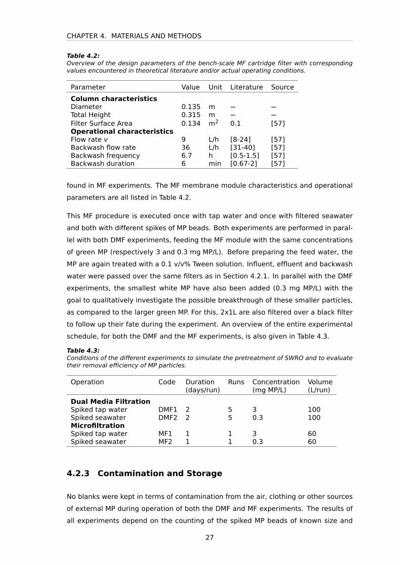
Table 4.2:Overview of the design parameters of the bench-scale MF cartridge filter with correspondingvalues encountered in theoretical literature and/or actual operating conditions.
Parameter Value Unit Literature Source
Column characteristicsDiameter 0.135 m − −Total Height 0.315 m − −Filter Surface Area 0.134 m2 0.1 [57]Operational characteristicsFlow rate v 9 L/h [8-24] [57]Backwash flow rate 36 L/h [31-40] [57]Backwash frequency 6.7 h [0.5-1.5] [57]Backwash duration 6 min [0.67-2] [57]
found in MF experiments. The MF membrane module characteristics and operational
parameters are all listed in Table 4.2.
This MF procedure is executed once with tap water and once with filtered seawater
and both with different spikes of MP beads. Both experiments are performed in paral-
lel with both DMF experiments, feeding the MF module with the same concentrations
of green MP (respectively 3 and 0.3 mg MP/L). Before preparing the feed water, the
MP are again treated with a 0.1 v/v% Tween solution. Influent, effluent and backwash
water were passed over the same filters as in Section 4.2.1. In parallel with the DMF
experiments, the smallest white MP have also been added (0.3 mg MP/L) with the
goal to qualitatively investigate the possible breakthrough of these smaller particles,
as compared to the larger green MP. For this, 2x1L are also filtered over a black filter
to follow up their fate during the experiment. An overview of the entire experimental
schedule, for both the DMF and the MF experiments, is also given in Table 4.3.
Table 4.3:Conditions of the different experiments to simulate the pretreatment of SWRO and to evaluatetheir removal efficiency of MP particles.
Operation Code Duration Runs Concentration Volume(days/run) (mg MP/L) (L/run)
Dual Media FiltrationSpiked tap water DMF1 2 5 3 100Spiked seawater DMF2 2 5 0.3 100MicrofiltrationSpiked tap water MF1 1 1 3 60Spiked seawater MF2 1 1 0.3 60
4.2.3 Contamination and Storage
No blanks were kept in terms of contamination from the air, clothing or other sources
of external MP during operation of both the DMF and MF experiments. The results of
all experiments depend on the counting of the spiked MP beads of known size and
27
4.2. SWRO PRETREATMENT SIMULATION
colour. These spikes are always of a high concentration and it is further assumed that
the contamination by external particles (plastic or other) of the same size and colour
is negligible.
The spatulas to place and remove the filter paper and the Buchner filter holder itself
are rinsed with demineralised water during every replacement of a filter paper. All
resulting filters are stored in fitting Petri dishes (90 mm) to prevent the loss of fil-
tered MP beads between collection and microscopic analysis. During the microscopy
analysis, blue nitrile gloves are worn to handle the filters. The glass surface of the
microscope is rinsed between every filter to prevent contamination of the spiked MP
beads between filters.
4.2.4 Microscopy Analysis
In the end, the performance of both the DMF and the MF set-up is followed up by
means of filtering the effluent and backwash streams, concentrating the spiked MP
on paper filters. Eventually, these filters are analysed by means of pictures taken by
a camera connected to a microscope and analysed through imaging software. The re-
sulting filters are analysed in two different ways, depending on a first visual inspection
of the filter. If none or barely any green MP are visually detectable, which is typical for
the effluent filters, the MP are counted individually by scanning the entire filter with
the microscope (Olympus SZX10 Stereo Microscope) and counting the plastic spheres
present one by one. This gives an exact number of MP present on a filter.
If filters (influent and backwash filters) contain many more particles after visual in-
spection, it is chosen to take microscopic pictures of the filter and further analyse
these with an imaging software to quantify the results. The reason for this alternative
method lies in the fact that the amount of MP is too high to count individually in these
cases.
4.2.5 Quantification and Counting Method
During this second part of the experimental research, the quantification of the re-
sults arises as a major challenge. Therefore, some additional analyses and tests are
performed to accurately quantify the results of the experiments. First of all, when
preparing the spiked feed water, the standardised MP are weighed down to an ac-
curacy of 1 mg. However, the resulting paper filters that contain the MP from the
different streams no longer allow weighing the plastics because it is possible that
other particles are present as well, especially on the backwash filters. Also, the accu-
racy would be very low to compare the different outcomes. In the end, as mentioned
28
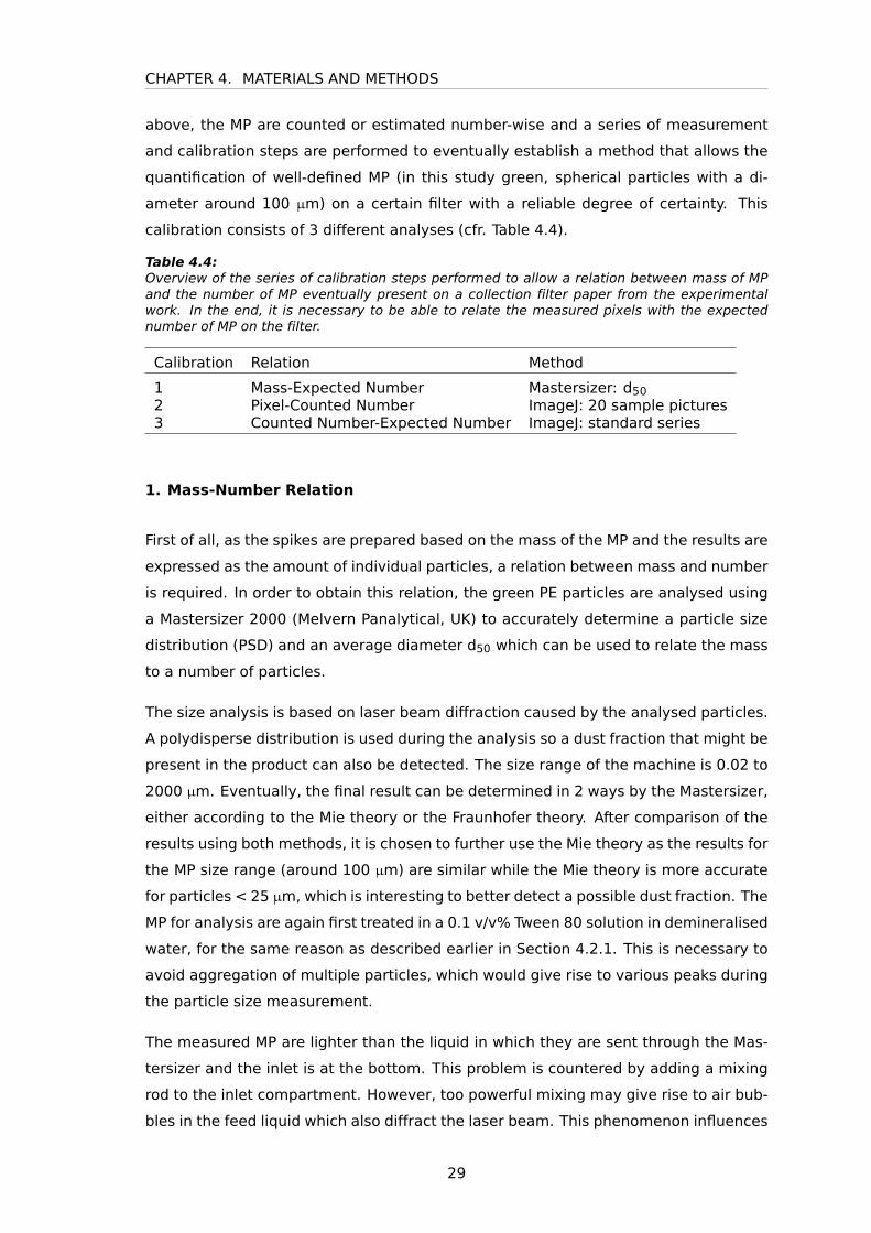
CHAPTER 4. MATERIALS AND METHODS
above, the MP are counted or estimated number-wise and a series of measurement
and calibration steps are performed to eventually establish a method that allows the
quantification of well-defined MP (in this study green, spherical particles with a di-
ameter around 100 µm) on a certain filter with a reliable degree of certainty. This
calibration consists of 3 different analyses (cfr. Table 4.4).
Table 4.4:Overview of the series of calibration steps performed to allow a relation between mass of MPand the number of MP eventually present on a collection filter paper from the experimentalwork. In the end, it is necessary to be able to relate the measured pixels with the expectednumber of MP on the filter.
Calibration Relation Method
1 Mass-Expected Number Mastersizer: d502 Pixel-Counted Number ImageJ: 20 sample pictures3 Counted Number-Expected Number ImageJ: standard series
1. Mass-Number Relation
First of all, as the spikes are prepared based on the mass of the MP and the results are
expressed as the amount of individual particles, a relation between mass and number
is required. In order to obtain this relation, the green PE particles are analysed using
a Mastersizer 2000 (Melvern Panalytical, UK) to accurately determine a particle size
distribution (PSD) and an average diameter d50 which can be used to relate the mass
to a number of particles.
The size analysis is based on laser beam diffraction caused by the analysed particles.
A polydisperse distribution is used during the analysis so a dust fraction that might be
present in the product can also be detected. The size range of the machine is 0.02 to
2000 µm. Eventually, the final result can be determined in 2 ways by the Mastersizer,
either according to the Mie theory or the Fraunhofer theory. After comparison of the
results using both methods, it is chosen to further use the Mie theory as the results for
the MP size range (around 100 µm) are similar while the Mie theory is more accurate
for particles < 25 µm, which is interesting to better detect a possible dust fraction. The
MP for analysis are again first treated in a 0.1 v/v% Tween 80 solution in demineralised
water, for the same reason as described earlier in Section 4.2.1. This is necessary to
avoid aggregation of multiple particles, which would give rise to various peaks during
the particle size measurement.
The measured MP are lighter than the liquid in which they are sent through the Mas-
tersizer and the inlet is at the bottom. This problem is countered by adding a mixing
rod to the inlet compartment. However, too powerful mixing may give rise to air bub-
bles in the feed liquid which also diffract the laser beam. This phenomenon influences
29
4.2. SWRO PRETREATMENT SIMULATION
the measurement as the air bubbles are also measured, typically as particles smaller
than the green MP size range.
The Mastersizer is typically operated in a closed system set-up, where the analysed
liquid is sent back to the feed compartment and is sent through the Mastersizer. This
leads to a second practical problem that is also related to the low density of the MP.
The relatively smaller particles stay in suspension longer that larger ones, which leads
to a bias towards smaller sizes as the smaller particles may be sent through the sys-
tem more frequently than large particles. For this reason, it is chosen to operate the
analysis as an open system. The analysed fraction is collected in a separate com-
partment and is not sent back through the system. This leads to a higher chance of
air bubbles as the liquid surface gradually decreases and approaches the mixing rod.
The solution for this issue consists eventually of manually adjusting the mixing rod to
avoid bubble production and intermittently interrupting the analysis to allow the bub-
bles to escape the feed liquid. The open system also implies interrupting the system
after every repetition and pouring the analysed liquid back in the feed compartment,
which gives rise to air bubbles again. This is countered by allowing enough time
between every analysis so bubbles can again escape the feed compartment before
starting up a new analysis.
2. Pixel-Number Relation
Secondly, it is necessary to establish a method to estimate the amount of particles
present on a filter when it is impossible to count them individually. In order to do this,
pictures are taken by means of a microscope and the surface that belongs to green
particles in terms of pixels is measured. This is possible as the camera connected
to the microscope always takes pictures from the same height and with the same
magnification. During this calibration, 20 random sample pictures are selected where
the amount of MP is in the order of magnitude of 10 to 100. Firstly, the MP are
counted visually on the picture. Then, the same picture is analysed using the imaging
software ImageJ (IJ 1.46r, USA). The processing of the images is explained below, in
Section 4.2.6. From this test, a relation between the average amount of pixels and
the corresponding amount of MP is obtained. In other words, it is determined how
many pixels 1 green MP occupies on average.
3. Evaluation of Counting Methods
Thirdly, another calibration test is designed to quantify the accuracy of a method
and to eventually select the best performing method. Two counting methods are
30
CHAPTER 4. MATERIALS AND METHODS
tested because the microscopic pictures are unable to cover the entire filter. Also,
the nature of the experiments leads to very heterogeneously spread patterns of MP
on the resulting filters, which complicates accurate estimates of the entire amount of
MP on one filter. The tested methods are: (1) 20 randomly taken pictures of known
and constant surface from which an average value is extracted and extrapolated to
the surface of the filer (= "Method 1"); and (2) 28 to 30 pictures of fixed parts that
cover the entire filter that are processed in a way that all results can eventually be
added up to estimate the total amount of MP present on the entire filter (= "Method
2"). The calibration test to evaluate the performance of both methods is based on
a series of 12 filters on which very precisely weighed amounts of the green MP, that
have been used throughout the experiments, are transferred. This standard series of
12 filters containing known amounts of MP is prepared and handled in the same way
as the experimental results. This allows to relate the estimated amount of MP with a
theoretically expected amount of MP based on the measured mass at the start so the
accuracy of a method can be evaluated.
4.2.6 Data Analysis
During the biofouling experiments, the density data are analysed using Microsoft Ex-
cel and the statistical software R. The ATP data are analysed using Microsoft Excel.
The results from the Mastersizer analyses, from which an average diameter (d50) is
extracted, are treated in Microsoft Excel. During the pretreatment simulations, the
resulting filters are processed and analysed using ImageJ. The processing consists of
cutting out the desired region of the picture and blurring out the noise inherent to the
background of the filter paper itself using the "Smoothen" function. Then, a colour
threshold was defined based on the HSB characteristics (Hue, Saturation and Bright-
ness) of the colours of a picture, every time set at respectively [70-135], [40-255]
and [0-255]. In this way, it is possible to selectively isolate the pixels of the green
beads from the background. The resulting pixels are related to an amount of MP by
means of the results of the performed calibrations. Further analysis of the results
is performed in Microsoft Excel. All data in Chapters 5 and 6 are reported with the
standard deviation.
31

4.2. SWRO PRETREATMENT SIMULATION
32
CHAPTER 5
RESULTS
5.1 Theoretical Considerations: Microplastic
Density and Water Density
Before presenting the results from the experimental work, some theoretical consid-
erations are made in relation with the density of MP and of the reject streams in the
SWRO process. MP density has been studied by following up the influence of bio-
fouling on a particle’s density (cfr. Section 5.2). The density difference between MP
particles and the SWRO reject streams will also return in Section 6.2 in a series of
simulation calculations concerning the SWRO process.
Table 2.1 shows polymers have different densities and they differ from the density
of water. Under normal conditions, all plastic particles will either float (lower den-
sity) or sink down (higher density). In this research, density will come forward as
an important parameter in the studied systems. Water density is variable and espe-
cially salt content and temperature exert an influence on this property (Figure 5.1).
However, temperature’s influence is much smaller than salt content’s influence. This
also means that the RO brine is denser than the backwash streams from the DMF
and/or MF in which the MP are retained. As a result, it might be possible to alter the
medium in which MP are present by mixing with the brine stream. Figure 5.2 relates
the density differences between pure water, seawater and RO brine with the densities
of different common polymers, as mentioned in Table 2.1. This shows that only two
types (PE and PP) are well below (sea)water’s density and that the brine from the
example calculation (Figure 2.4) is not that much denser in the sense that it possibly
only includes one more polymer type (PS). It appears that density differences of poly-
mers are too big in relation to the increase in density of seawater after concentrating
the salts during the RO process. This points in the direction that a direct application
of this waste stream will not produce an added value in the search for a cost-effective
removal of MP from the SWRO reject streams. This will be further discussed during
the simulation calculations in Section 6.2.
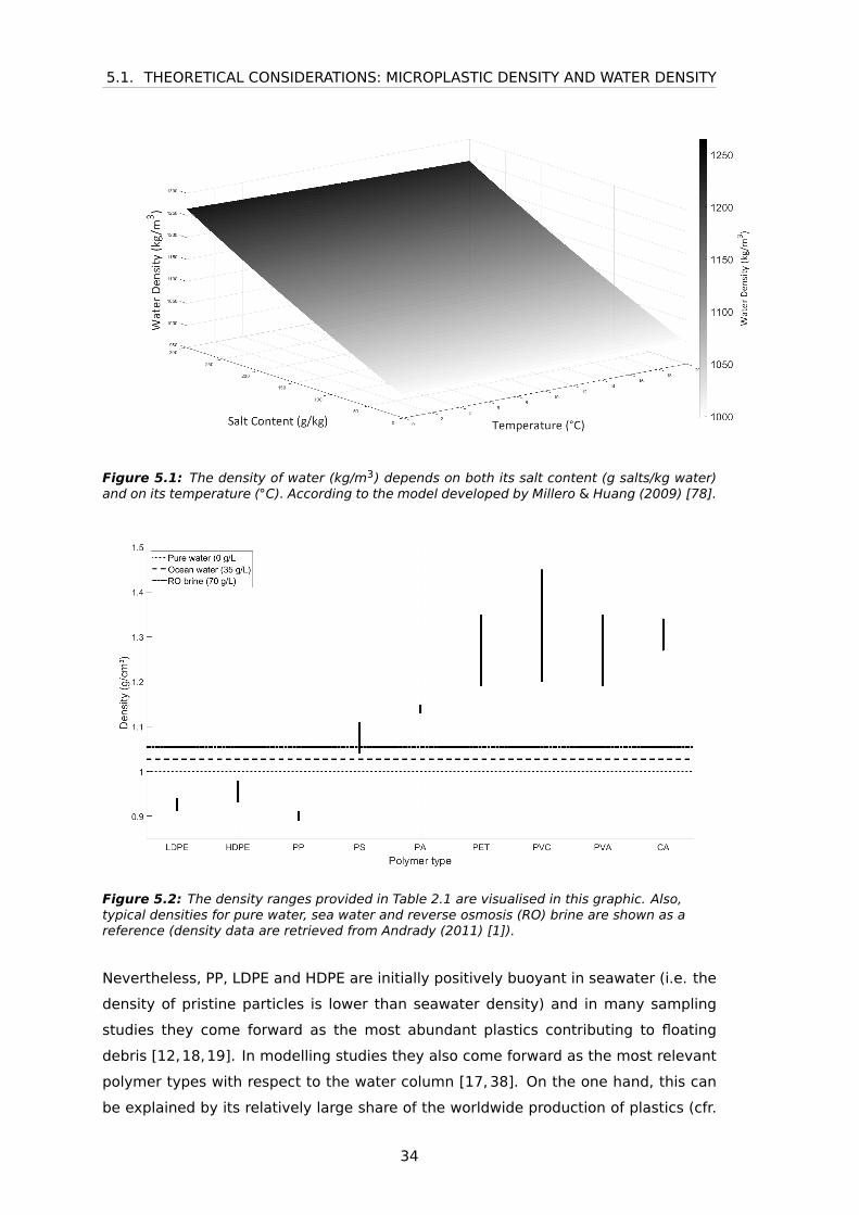
5.1. THEORETICAL CONSIDERATIONS: MICROPLASTIC DENSITY AND WATER DENSITY
Figure 5.1: The density of water (kg/m3) depends on both its salt content (g salts/kg water)and on its temperature (◦C). According to the model developed by Millero & Huang (2009) [78].
Figure 5.2: The density ranges provided in Table 2.1 are visualised in this graphic. Also,typical densities for pure water, sea water and reverse osmosis (RO) brine are shown as areference (density data are retrieved from Andrady (2011) [1]).
Nevertheless, PP, LDPE and HDPE are initially positively buoyant in seawater (i.e. the
density of pristine particles is lower than seawater density) and in many sampling
studies they come forward as the most abundant plastics contributing to floating
debris [12,18,19]. In modelling studies they also come forward as the most relevant
polymer types with respect to the water column [17,38]. On the one hand, this can
be explained by its relatively large share of the worldwide production of plastics (cfr.
34
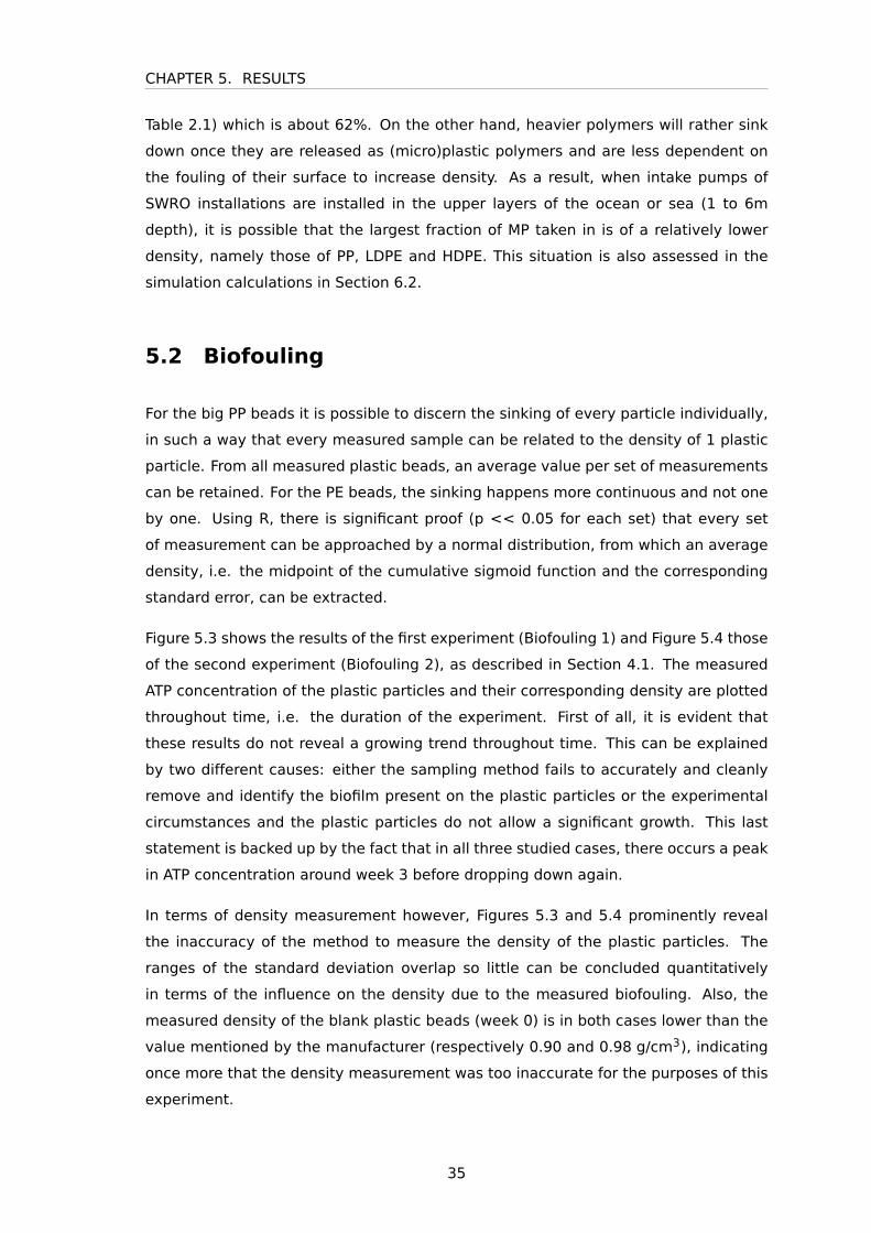
CHAPTER 5. RESULTS
Table 2.1) which is about 62%. On the other hand, heavier polymers will rather sink
down once they are released as (micro)plastic polymers and are less dependent on
the fouling of their surface to increase density. As a result, when intake pumps of
SWRO installations are installed in the upper layers of the ocean or sea (1 to 6m
depth), it is possible that the largest fraction of MP taken in is of a relatively lower
density, namely those of PP, LDPE and HDPE. This situation is also assessed in the
simulation calculations in Section 6.2.
5.2 Biofouling
For the big PP beads it is possible to discern the sinking of every particle individually,
in such a way that every measured sample can be related to the density of 1 plastic
particle. From all measured plastic beads, an average value per set of measurements
can be retained. For the PE beads, the sinking happens more continuous and not one
by one. Using R, there is significant proof (p << 0.05 for each set) that every set
of measurement can be approached by a normal distribution, from which an average
density, i.e. the midpoint of the cumulative sigmoid function and the corresponding
standard error, can be extracted.
Figure 5.3 shows the results of the first experiment (Biofouling 1) and Figure 5.4 those
of the second experiment (Biofouling 2), as described in Section 4.1. The measured
ATP concentration of the plastic particles and their corresponding density are plotted
throughout time, i.e. the duration of the experiment. First of all, it is evident that
these results do not reveal a growing trend throughout time. This can be explained
by two different causes: either the sampling method fails to accurately and cleanly
remove and identify the biofilm present on the plastic particles or the experimental
circumstances and the plastic particles do not allow a significant growth. This last
statement is backed up by the fact that in all three studied cases, there occurs a peak
in ATP concentration around week 3 before dropping down again.
In terms of density measurement however, Figures 5.3 and 5.4 prominently reveal
the inaccuracy of the method to measure the density of the plastic particles. The
ranges of the standard deviation overlap so little can be concluded quantitatively
in terms of the influence on the density due to the measured biofouling. Also, the
measured density of the blank plastic beads (week 0) is in both cases lower than the
value mentioned by the manufacturer (respectively 0.90 and 0.98 g/cm3), indicating
once more that the density measurement was too inaccurate for the purposes of this
experiment.
35

5.2. BIOFOULING
(a) The results of the Biofouling 1 experiment for the PP particles throughout time. For weeks 0, 1, 2, 4 and6 samples have been analysed for density and ATP concentration. The error bars represent the standarddeviation between measurements of either density or ATP concentration. If n represents the number ofrepetitions per measurement, then n=10 and n=30 respectively.
(b) As for (a) but with the smaller PE particles. n=40 and n=30, for density and ATP concentration mea-surement respectively.
Figure 5.3: Results of the Biofouling 1 experiments for both the PP (a) and PE (b) beads.
Lastly, Figure 5.5 shows the same results as Figure 5.3a for the PP particles but now
the time factor is eliminated. Once again, it is clear that the vertical error bars, i.e. the
deviation on the density measurement, are too big. Yet, the results show an apparent
36
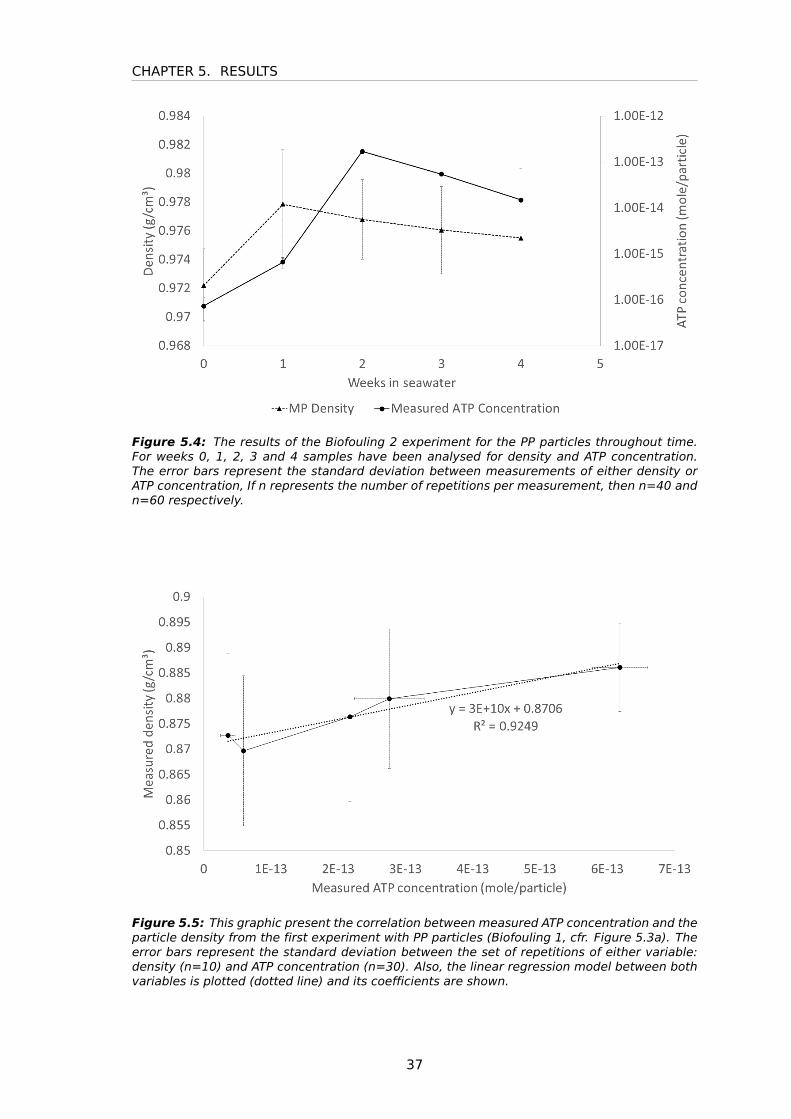
CHAPTER 5. RESULTS
Figure 5.4: The results of the Biofouling 2 experiment for the PP particles throughout time.For weeks 0, 1, 2, 3 and 4 samples have been analysed for density and ATP concentration.The error bars represent the standard deviation between measurements of either density orATP concentration, If n represents the number of repetitions per measurement, then n=40 andn=60 respectively.
Figure 5.5: This graphic present the correlation between measured ATP concentration and theparticle density from the first experiment with PP particles (Biofouling 1, cfr. Figure 5.3a). Theerror bars represent the standard deviation between the set of repetitions of either variable:density (n=10) and ATP concentration (n=30). Also, the linear regression model between bothvariables is plotted (dotted line) and its coefficients are shown.
37
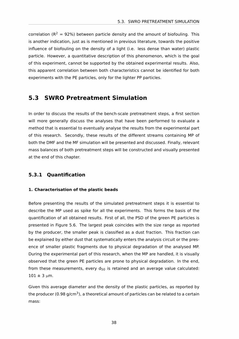
5.3. SWRO PRETREATMENT SIMULATION
correlation (R2 = 92%) between particle density and the amount of biofouling. This
is another indication, just as is mentioned in previous literature, towards the positive
influence of biofouling on the density of a light (i.e. less dense than water) plastic
particle. However, a quantitative description of this phenomenon, which is the goal
of this experiment, cannot be supported by the obtained experimental results. Also,
this apparent correlation between both characteristics cannot be identified for both
experiments with the PE particles, only for the lighter PP particles.
5.3 SWRO Pretreatment Simulation
In order to discuss the results of the bench-scale pretreatment steps, a first section
will more generally discuss the analyses that have been performed to evaluate a
method that is essential to eventually analyse the results from the experimental part
of this research. Secondly, these results of the different streams containing MP of
both the DMF and the MF simulation will be presented and discussed. Finally, relevant
mass balances of both pretreatment steps will be constructed and visually presented
at the end of this chapter.
5.3.1 Quantification
1. Characterisation of the plastic beads
Before presenting the results of the simulated pretreatment steps it is essential to
describe the MP used as spike for all the experiments. This forms the basis of the
quantification of all obtained results. First of all, the PSD of the green PE particles is
presented in Figure 5.6. The largest peak coincides with the size range as reported
by the producer, the smaller peak is classified as a dust fraction. This fraction can
be explained by either dust that systematically enters the analysis circuit or the pres-
ence of smaller plastic fragments due to physical degradation of the analysed MP.
During the experimental part of this research, when the MP are handled, it is visually
observed that the green PE particles are prone to physical degradation. In the end,
from these measurements, every d50 is retained and an average value calculated:
101 ± 3 µm.
Given this average diameter and the density of the plastic particles, as reported by
the producer (0.98 g/cm3), a theoretical amount of particles can be related to a certain
mass:
38
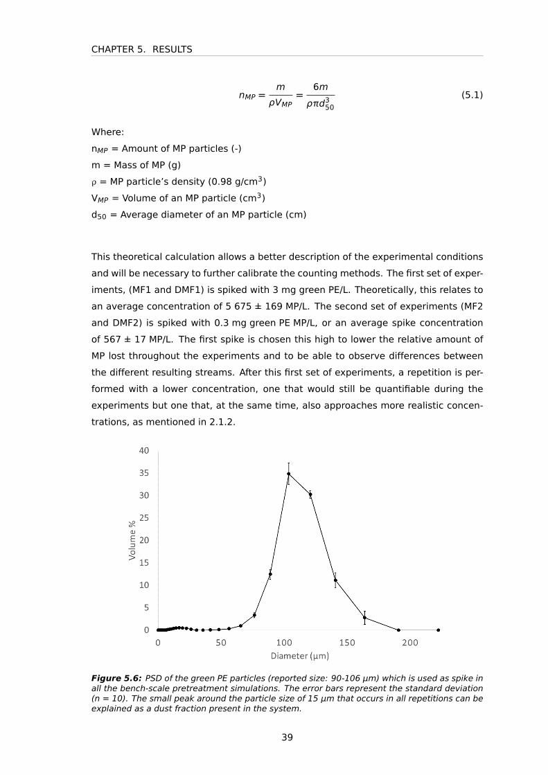
CHAPTER 5. RESULTS
nMP =m
ρVMP=
6m
ρπd350(5.1)
Where:
nMP = Amount of MP particles (-)
m = Mass of MP (g)
ρ = MP particle’s density (0.98 g/cm3)
VMP = Volume of an MP particle (cm3)
d50 = Average diameter of an MP particle (cm)
This theoretical calculation allows a better description of the experimental conditions
and will be necessary to further calibrate the counting methods. The first set of exper-
iments, (MF1 and DMF1) is spiked with 3 mg green PE/L. Theoretically, this relates to
an average concentration of 5 675 ± 169 MP/L. The second set of experiments (MF2
and DMF2) is spiked with 0.3 mg green PE MP/L, or an average spike concentration
of 567 ± 17 MP/L. The first spike is chosen this high to lower the relative amount of
MP lost throughout the experiments and to be able to observe differences between
the different resulting streams. After this first set of experiments, a repetition is per-
formed with a lower concentration, one that would still be quantifiable during the
experiments but one that, at the same time, also approaches more realistic concen-
trations, as mentioned in 2.1.2.
Figure 5.6: PSD of the green PE particles (reported size: 90-106 μm) which is used as spike inall the bench-scale pretreatment simulations. The error bars represent the standard deviation(n = 10). The small peak around the particle size of 15 μm that occurs in all repetitions can beexplained as a dust fraction present in the system.
39
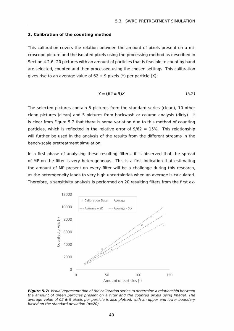
5.3. SWRO PRETREATMENT SIMULATION
2. Calibration of the counting method
This calibration covers the relation between the amount of pixels present on a mi-
croscope picture and the isolated pixels using the processing method as described in
Section 4.2.6. 20 pictures with an amount of particles that is feasible to count by hand
are selected, counted and then processed using the chosen settings. This calibration
gives rise to an average value of 62 ± 9 pixels (Y) per particle (X):
Y = (62 ± 9)X (5.2)
The selected pictures contain 5 pictures from the standard series (clean), 10 other
clean pictures (clean) and 5 pictures from backwash or column analysis (dirty). It
is clear from Figure 5.7 that there is some variation due to this method of counting
particles, which is reflected in the relative error of 9/62 = 15%. This relationship
will further be used in the analysis of the results from the different streams in the
bench-scale pretreatment simulation.
In a first phase of analysing these resulting filters, it is observed that the spread
of MP on the filter is very heterogeneous. This is a first indication that estimating
the amount of MP present on every filter will be a challenge during this research,
as the heterogeneity leads to very high uncertainties when an average is calculated.
Therefore, a sensitivity analysis is performed on 20 resulting filters from the first ex-
Figure 5.7: Visual representation of the calibration series to determine a relationship betweenthe amount of green particles present on a filter and the counted pixels using ImageJ. Theaverage value of 62 ± 9 pixels per particle is also plotted, with an upper and lower boundarybased on the standard deviation (n=20).
40
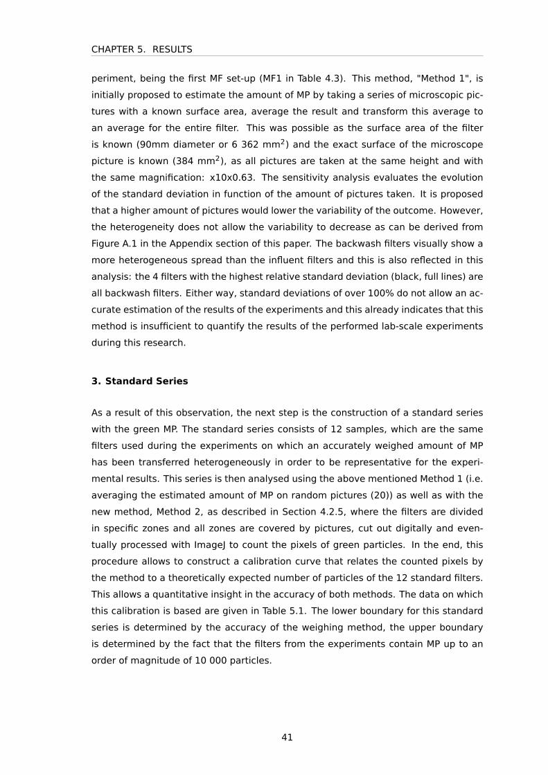
CHAPTER 5. RESULTS
periment, being the first MF set-up (MF1 in Table 4.3). This method, "Method 1", is
initially proposed to estimate the amount of MP by taking a series of microscopic pic-
tures with a known surface area, average the result and transform this average to
an average for the entire filter. This was possible as the surface area of the filter
is known (90mm diameter or 6 362 mm2) and the exact surface of the microscope
picture is known (384 mm2), as all pictures are taken at the same height and with
the same magnification: x10x0.63. The sensitivity analysis evaluates the evolution
of the standard deviation in function of the amount of pictures taken. It is proposed
that a higher amount of pictures would lower the variability of the outcome. However,
the heterogeneity does not allow the variability to decrease as can be derived from
Figure A.1 in the Appendix section of this paper. The backwash filters visually show a
more heterogeneous spread than the influent filters and this is also reflected in this
analysis: the 4 filters with the highest relative standard deviation (black, full lines) are
all backwash filters. Either way, standard deviations of over 100% do not allow an ac-
curate estimation of the results of the experiments and this already indicates that this
method is insufficient to quantify the results of the performed lab-scale experiments
during this research.
3. Standard Series
As a result of this observation, the next step is the construction of a standard series
with the green MP. The standard series consists of 12 samples, which are the same
filters used during the experiments on which an accurately weighed amount of MP
has been transferred heterogeneously in order to be representative for the experi-
mental results. This series is then analysed using the above mentioned Method 1 (i.e.
averaging the estimated amount of MP on random pictures (20)) as well as with the
new method, Method 2, as described in Section 4.2.5, where the filters are divided
in specific zones and all zones are covered by pictures, cut out digitally and even-
tually processed with ImageJ to count the pixels of green particles. In the end, this
procedure allows to construct a calibration curve that relates the counted pixels by
the method to a theoretically expected number of particles of the 12 standard filters.
This allows a quantitative insight in the accuracy of both methods. The data on which
this calibration is based are given in Table 5.1. The lower boundary for this standard
series is determined by the accuracy of the weighing method, the upper boundary
is determined by the fact that the filters from the experiments contain MP up to an
order of magnitude of 10 000 particles.
41
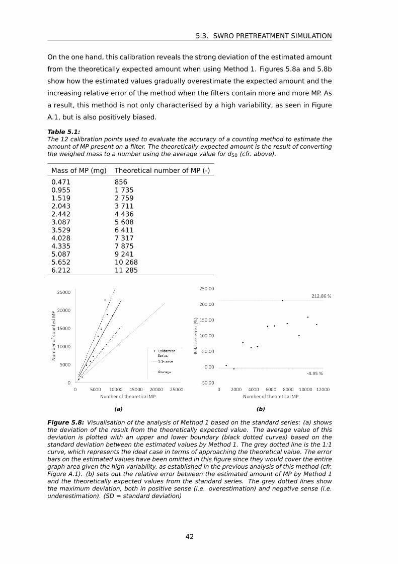
5.3. SWRO PRETREATMENT SIMULATION
On the one hand, this calibration reveals the strong deviation of the estimated amount
from the theoretically expected amount when using Method 1. Figures 5.8a and 5.8b
show how the estimated values gradually overestimate the expected amount and the
increasing relative error of the method when the filters contain more and more MP. As
a result, this method is not only characterised by a high variability, as seen in Figure
A.1, but is also positively biased.
Table 5.1:The 12 calibration points used to evaluate the accuracy of a counting method to estimate theamount of MP present on a filter. The theoretically expected amount is the result of convertingthe weighed mass to a number using the average value for d50 (cfr. above).
Mass of MP (mg) Theoretical number of MP (-)
0.471 8560.955 1 7351.519 2 7592.043 3 7112.442 4 4363.087 5 6083.529 6 4114.028 7 3174.335 7 8755.087 9 2415.652 10 2686.212 11 285
(a) (b)
Figure 5.8: Visualisation of the analysis of Method 1 based on the standard series: (a) showsthe deviation of the result from the theoretically expected value. The average value of thisdeviation is plotted with an upper and lower boundary (black dotted curves) based on thestandard deviation between the estimated values by Method 1. The grey dotted line is the 1:1curve, which represents the ideal case in terms of approaching the theoretical value. The errorbars on the estimated values have been omitted in this figure since they would cover the entiregraph area given the high variability, as established in the previous analysis of this method (cfr.Figure A.1). (b) sets out the relative error between the estimated amount of MP by Method 1and the theoretically expected values from the standard series. The grey dotted lines showthe maximum deviation, both in positive sense (i.e. overestimation) and negative sense (i.e.underestimation). (SD = standard deviation)
42
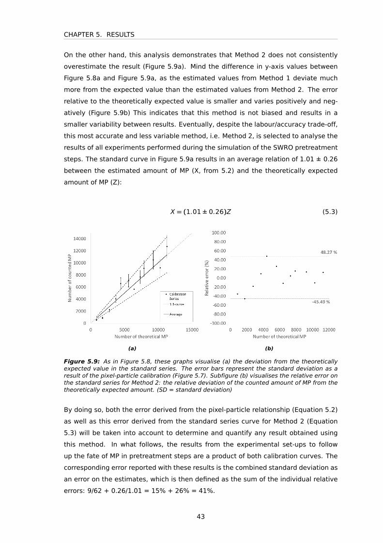
CHAPTER 5. RESULTS
On the other hand, this analysis demonstrates that Method 2 does not consistently
overestimate the result (Figure 5.9a). Mind the difference in y-axis values between
Figure 5.8a and Figure 5.9a, as the estimated values from Method 1 deviate much
more from the expected value than the estimated values from Method 2. The error
relative to the theoretically expected value is smaller and varies positively and neg-
atively (Figure 5.9b) This indicates that this method is not biased and results in a
smaller variability between results. Eventually, despite the labour/accuracy trade-off,
this most accurate and less variable method, i.e. Method 2, is selected to analyse the
results of all experiments performed during the simulation of the SWRO pretreatment
steps. The standard curve in Figure 5.9a results in an average relation of 1.01 ± 0.26
between the estimated amount of MP (X, from 5.2) and the theoretically expected
amount of MP (Z):
X = (1.01 ± 0.26)Z (5.3)
(a) (b)
Figure 5.9: As in Figure 5.8, these graphs visualise (a) the deviation from the theoreticallyexpected value in the standard series. The error bars represent the standard deviation as aresult of the pixel-particle calibration (Figure 5.7). Subfigure (b) visualises the relative error onthe standard series for Method 2: the relative deviation of the counted amount of MP from thetheoretically expected amount. (SD = standard deviation)
By doing so, both the error derived from the pixel-particle relationship (Equation 5.2)
as well as this error derived from the standard series curve for Method 2 (Equation
5.3) will be taken into account to determine and quantify any result obtained using
this method. In what follows, the results from the experimental set-ups to follow
up the fate of MP in pretreatment steps are a product of both calibration curves. The
corresponding error reported with these results is the combined standard deviation as
an error on the estimates, which is then defined as the sum of the individual relative
errors: 9/62 + 0.26/1.01 = 15% + 26% = 41%.
43
5.3. SWRO PRETREATMENT SIMULATION
5.3.2 Dual Media Filtration
DMF Influent
As mentioned in the previous chapter (Section 4.2.1), empty column runs are per-
formed to better estimate the actual flux of MP that passes through the constructed
system, rather than relying on the mass of MP that is added as spike to the feed tank.
For both the DMF1 and DMF2 experiments (spiked with respectively 3 and 0.3 mg
MP/L, cfr. Table 4.3), 1 empty run of 100L was performed. This results in an average
ingoing flux of 5 491 ± 2 249 and 676 ± 277 MP/L, respectively. These values will
further act as the reference influent concentration to define removal efficiencies and
corresponding mass balances.
DMF Effluent
One of the main interests in this research is to identify the pretreatment steps that
retain MP during their operation. All effluent filters appear to contain little to none
MP after visual inspection, which implies that the result is counted by the naked eye
using a microscope. The results are listed in Table 5.2. The removal efficiencies of
the spiked green MP during both DMF experiments reach 99.9%. In a previous study
with the combination anthracite-sand no breakthrough was observed, however,in this
case, only a 2L spike was fed to the filter. After the long-term operation of 10 days
in this study, a minimal breakthrough of MP is observed, which is in line with the
previous finding [68]. Mind that both DMF experiments have been performed with
fresh filter material (anthracite and sand) as it is removed after each experiment for
the analysis of the filter material itself.
In Section 4.2.1, it is mentioned that in the second experiment (DMF 2), an additional
spike of 0.3 mg/L of white MP is added to the influent of the DMF set-up. These white
MP are smaller than the green MP spike, with a reported size of 10 to 45 µm. As
no method is developed to accurately count these MP in the resulting streams, their
quantification is no goal of this experimental research. However, 2 times 1L of every
run of 100L is collected over black filter paper to be used for a qualitative indication
for breakthrough of these smaller MP. However, on none of the 10 (2x5) black filter
papers from this experiment a white MP is found after microscopic analysis. Without
any further ground for conclusions, this is an indication that smaller MP, with a size
range close to the lower boundary of MP, are possibly also well retained by the DMF
set-up. This will be further discussed at the end of this study in Section 7.1.
44
CHAPTER 5. RESULTS
Table 5.2:Overview of the analysis of the effluent filters for both DMF simulation experiments (1 run =100L). The removal efficiency per run is expressed as a fraction of the average influent of theDMF 1 and the DMF 2 experiments, respectively 5 491 and 676 MP/L. The number of MP in thesecond column are counted manually and no standard deviation is reported for those values.(SD = standard deviation)
Run Number of MP Concentration Removal SD(-) (MP/L) Efficiency (%) (%)
DMF 11 5 0.05 99.999 ± 0.00042 3 0.03 99.999 ± 0.00023 56 0.56 99.990 ± 0.00424 19 0.19 99.997 ± 0.00145 42 0.42 99.992 ± 0.0031Average 25 0.25 99.995 ± 0.0093
DMF 21 30 0.30 99.956 ± 0.0182 3 0.03 99.996 ± 0.0023 2 0.02 99.997 ± 0.0014 1 0.01 99.999 ± 0.0015 0 0 100 ± 0.001Average 7.2 0.072 99.989 ± 0.022
DMF Backwash Procedure
After each of the first 4 runs out of 5 in total of every DMF experiment, a backwash
procedure is performed. The resulting backwash stream with washed out contami-
nants and MP is again collected on filters. Given the design parameters, a backwash
procedure lasts 10 minutes and 6L of water is sent bottom-to-top through the column,
which is eventually collected on a series of 6 filters (i.e. 1L is passed over each filter).
Figure 5.10 visualises these 8 backwash procedures: 4 times for each experiment
(respectively 5.10a and 5.10b). The values are expressed as the fraction of the total
amount of MP that is washed out during each procedure (i.e. all 6 bars of a certain
backwash add up to 100%). These results show that most of the washed out MP
detach from the filter material easily. In 6 out of 8 cases, observed over both experi-
ments, at least 50% of the total amount washed out during a backwash procedure is
removed in the first minutes, contained in the first litre of backwash water.
In response to Figure 5.10a (DMF 1), two additional remarks are necessary. First of all,
during the very first procedure ("Backwash 1" in DMF 1, black bars), the backwash is
performed poorly. The filter material does not expand and the water passes through
the filter material as if it were a regular sand filter. This explains the more uniform
washing out of the MP that can be observed. Also, as will be shown in Table 5.3,
the total amount of MP washed out is the lowest during this backwash procedure,
indicating its poor execution compared to the other backwash procedures.
45
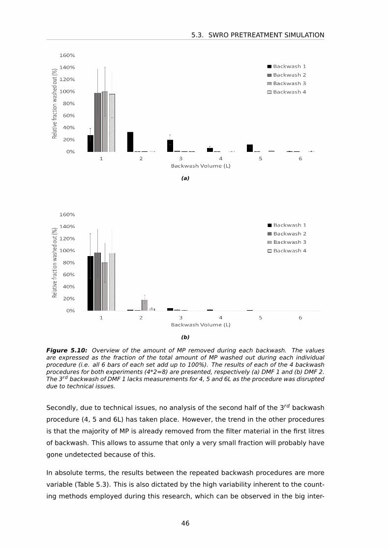
5.3. SWRO PRETREATMENT SIMULATION
(a)
(b)
Figure 5.10: Overview of the amount of MP removed during each backwash. The valuesare expressed as the fraction of the total amount of MP washed out during each individualprocedure (i.e. all 6 bars of each set add up to 100%). The results of each of the 4 backwashprocedures for both experiments (4*2=8) are presented, respectively (a) DMF 1 and (b) DMF 2.The 3rd backwash of DMF 1 lacks measurements for 4, 5 and 6L as the procedure was disrupteddue to technical issues.
Secondly, due to technical issues, no analysis of the second half of the 3rd backwash
procedure (4, 5 and 6L) has taken place. However, the trend in the other procedures
is that the majority of MP is already removed from the filter material in the first litres
of backwash. This allows to assume that only a very small fraction will probably have
gone undetected because of this.
In absolute terms, the results between the repeated backwash procedures are more
variable (Table 5.3). This is also dictated by the high variability inherent to the count-
ing methods employed during this research, which can be observed in the big inter-
46
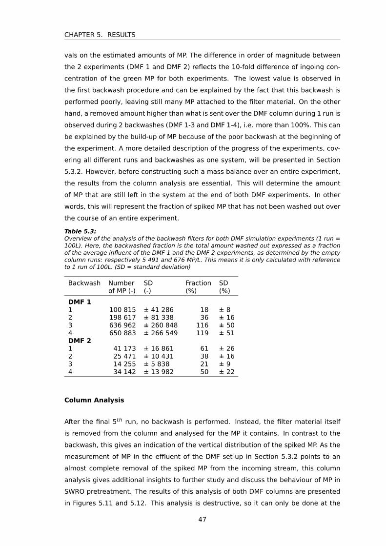
CHAPTER 5. RESULTS
vals on the estimated amounts of MP. The difference in order of magnitude between
the 2 experiments (DMF 1 and DMF 2) reflects the 10-fold difference of ingoing con-
centration of the green MP for both experiments. The lowest value is observed in
the first backwash procedure and can be explained by the fact that this backwash is
performed poorly, leaving still many MP attached to the filter material. On the other
hand, a removed amount higher than what is sent over the DMF column during 1 run is
observed during 2 backwashes (DMF 1-3 and DMF 1-4), i.e. more than 100%. This can
be explained by the build-up of MP because of the poor backwash at the beginning of
the experiment. A more detailed description of the progress of the experiments, cov-
ering all different runs and backwashes as one system, will be presented in Section
5.3.2. However, before constructing such a mass balance over an entire experiment,
the results from the column analysis are essential. This will determine the amount
of MP that are still left in the system at the end of both DMF experiments. In other
words, this will represent the fraction of spiked MP that has not been washed out over
the course of an entire experiment.
Table 5.3:Overview of the analysis of the backwash filters for both DMF simulation experiments (1 run =100L). Here, the backwashed fraction is the total amount washed out expressed as a fractionof the average influent of the DMF 1 and the DMF 2 experiments, as determined by the emptycolumn runs: respectively 5 491 and 676 MP/L. This means it is only calculated with referenceto 1 run of 100L. (SD = standard deviation)
Backwash Number SD Fraction SDof MP (-) (-) (%) (%)
DMF 11 100 815 ± 41 286 18 ± 82 198 617 ± 81 338 36 ± 163 636 962 ± 260 848 116 ± 504 650 883 ± 266 549 119 ± 51DMF 21 41 173 ± 16 861 61 ± 262 25 471 ± 10 431 38 ± 163 14 255 ± 5 838 21 ± 94 34 142 ± 13 982 50 ± 22
Column Analysis
After the final 5th run, no backwash is performed. Instead, the filter material itself
is removed from the column and analysed for the MP it contains. In contrast to the
backwash, this gives an indication of the vertical distribution of the spiked MP. As the
measurement of MP in the effluent of the DMF set-up in Section 5.3.2 points to an
almost complete removal of the spiked MP from the incoming stream, this column
analysis gives additional insights to further study and discuss the behaviour of MP in
SWRO pretreatment. The results of this analysis of both DMF columns are presented
in Figures 5.11 and 5.12. This analysis is destructive, so it can only be done at the
47
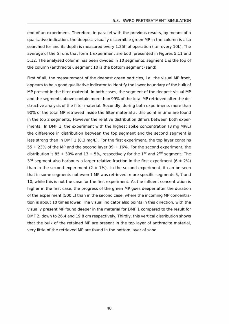
5.3. SWRO PRETREATMENT SIMULATION
end of an experiment. Therefore, in parallel with the previous results, by means of a
qualitative indication, the deepest visually discernible green MP in the column is also
searched for and its depth is measured every 1.25h of operation (i.e. every 10L). The
average of the 5 runs that form 1 experiment are both presented in Figures 5.11 and
5.12. The analysed column has been divided in 10 segments, segment 1 is the top of
the column (anthracite), segment 10 is the bottom segment (sand).
First of all, the measurement of the deepest green particles, i.e. the visual MP front,
appears to be a good qualitative indicator to identify the lower boundary of the bulk of
MP present in the filter material. In both cases, the segment of the deepest visual MP
and the segments above contain more than 99% of the total MP retrieved after the de-
structive analysis of the filter material. Secondly, during both experiments more than
90% of the total MP retrieved inside the filter material at this point in time are found
in the top 2 segments. However the relative distribution differs between both exper-
iments. In DMF 1, the experiment with the highest spike concentration (3 mg MP/L)
the difference in distribution between the top segment and the second segment is
less strong than in DMF 2 (0.3 mg/L). For the first experiment, the top layer contains
55 ± 23% of the MP and the second layer 39 ± 16%. For the second experiment, the
distribution is 85 ± 30% and 13 ± 5%, respectively for the 1st and 2nd segment. The
3rd segment also harbours a larger relative fraction in the first experiment (6 ± 2%)
than in the second experiment (2 ± 1%). In the second experiment, it can be seen
that in some segments not even 1 MP was retrieved, more specific segments 5, 7 and
10, while this is not the case for the first experiment. As the influent concentration is
higher in the first case, the progress of the green MP goes deeper after the duration
of the experiment (500 L) than in the second case, where the incoming MP concentra-
tion is about 10 times lower. The visual indicator also points in this direction, with the
visually present MP found deeper in the material for DMF 1 compared to the result for
DMF 2, down to 26.4 and 19.8 cm respectively. Thirdly, this vertical distribution shows
that the bulk of the retained MP are present in the top layer of anthracite material,
very little of the retrieved MP are found in the bottom layer of sand.
48
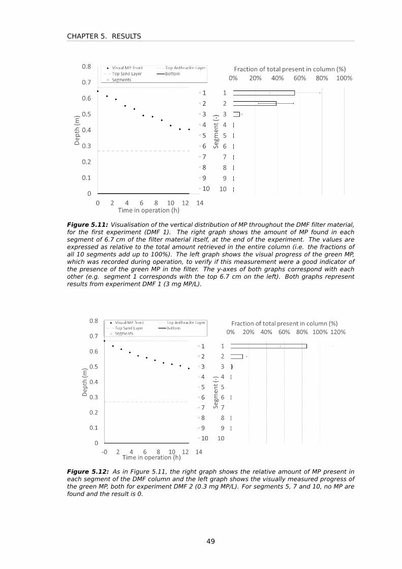
CHAPTER 5. RESULTS
Figure 5.11: Visualisation of the vertical distribution of MP throughout the DMF filter material,for the first experiment (DMF 1). The right graph shows the amount of MP found in eachsegment of 6.7 cm of the filter material itself, at the end of the experiment. The values areexpressed as relative to the total amount retrieved in the entire column (i.e. the fractions ofall 10 segments add up to 100%). The left graph shows the visual progress of the green MP,which was recorded during operation, to verify if this measurement were a good indicator ofthe presence of the green MP in the filter. The y-axes of both graphs correspond with eachother (e.g. segment 1 corresponds with the top 6.7 cm on the left). Both graphs representresults from experiment DMF 1 (3 mg MP/L).
Figure 5.12: As in Figure 5.11, the right graph shows the relative amount of MP present ineach segment of the DMF column and the left graph shows the visually measured progress ofthe green MP, both for experiment DMF 2 (0.3 mg MP/L). For segments 5, 7 and 10, no MP arefound and the result is 0.
49
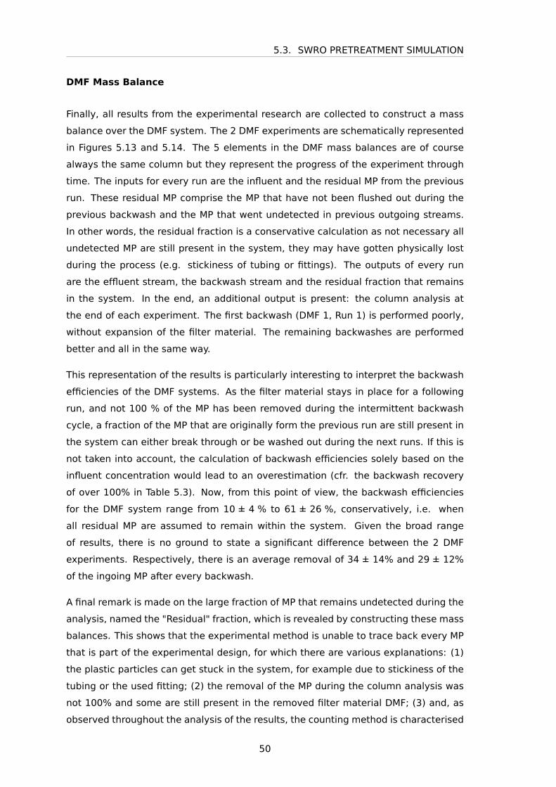
5.3. SWRO PRETREATMENT SIMULATION
DMF Mass Balance
Finally, all results from the experimental research are collected to construct a mass
balance over the DMF system. The 2 DMF experiments are schematically represented
in Figures 5.13 and 5.14. The 5 elements in the DMF mass balances are of course
always the same column but they represent the progress of the experiment through
time. The inputs for every run are the influent and the residual MP from the previous
run. These residual MP comprise the MP that have not been flushed out during the
previous backwash and the MP that went undetected in previous outgoing streams.
In other words, the residual fraction is a conservative calculation as not necessary all
undetected MP are still present in the system, they may have gotten physically lost
during the process (e.g. stickiness of tubing or fittings). The outputs of every run
are the effluent stream, the backwash stream and the residual fraction that remains
in the system. In the end, an additional output is present: the column analysis at
the end of each experiment. The first backwash (DMF 1, Run 1) is performed poorly,
without expansion of the filter material. The remaining backwashes are performed
better and all in the same way.
This representation of the results is particularly interesting to interpret the backwash
efficiencies of the DMF systems. As the filter material stays in place for a following
run, and not 100 % of the MP has been removed during the intermittent backwash
cycle, a fraction of the MP that are originally form the previous run are still present in
the system can either break through or be washed out during the next runs. If this is
not taken into account, the calculation of backwash efficiencies solely based on the
influent concentration would lead to an overestimation (cfr. the backwash recovery
of over 100% in Table 5.3). Now, from this point of view, the backwash efficiencies
for the DMF system range from 10 ± 4 % to 61 ± 26 %, conservatively, i.e. when
all residual MP are assumed to remain within the system. Given the broad range
of results, there is no ground to state a significant difference between the 2 DMF
experiments. Respectively, there is an average removal of 34 ± 14% and 29 ± 12%
of the ingoing MP after every backwash.
A final remark is made on the large fraction of MP that remains undetected during the
analysis, named the "Residual" fraction, which is revealed by constructing these mass
balances. This shows that the experimental method is unable to trace back every MP
that is part of the experimental design, for which there are various explanations: (1)
the plastic particles can get stuck in the system, for example due to stickiness of the
tubing or the used fitting; (2) the removal of the MP during the column analysis was
not 100% and some are still present in the removed filter material DMF; (3) and, as
observed throughout the analysis of the results, the counting method is characterised
50
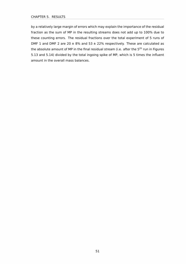
CHAPTER 5. RESULTS
by a relatively large margin of errors which may explain the importance of the residual
fraction as the sum of MP in the resulting streams does not add up to 100% due to
these counting errors. The residual fractions over the total experiment of 5 runs of
DMF 1 and DMF 2 are 20 ± 8% and 53 ± 22% respectively. These are calculated as
the absolute amount of MP in the final residual stream (i.e. after the 5th run in Figures
5.13 and 5.14) divided by the total ingoing spike of MP, which is 5 times the influent
amount in the overall mass balances.
51
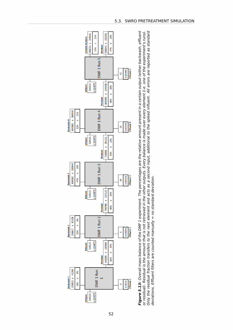
5.3. SWRO PRETREATMENT SIMULATION
Figure
5.13:
Ove
rall
mas
sbal
ance
ofth
eD
MF
1ex
per
imen
t.Th
eper
centa
ges
are
the
rela
tive
amou
nt
pre
sent
ina
cert
ain
outp
ut
(eit
her
bac
kwas
h,e
ffluen
tor
resi
dual
).R
esid
ual
isth
eam
ount
that
isnot
retr
ieve
din
the
other
outp
uts
.Eve
rybal
ance
ism
ade
over
ever
yel
emen
t(i
.e.
one
ofth
eex
per
imen
t’s
runs)
.O
nly
the
resi
dual
frac
tion
tran
sfer
sto
the
nex
tel
emen
tan
dac
tsas
ase
cond
input,
addit
ional
toth
esp
iked
infl
uen
t.A
ller
rors
are
repor
ted
asst
andar
ddev
iati
ons.
Effl
uen
tfi
lter
sar
eco
unte
dm
anual
ly=
no
stan
dar
ddev
iati
on.
52
CHAPTER 5. RESULTS
Figure
5.14:
Ove
rall
mas
sbal
ance
ofth
eD
MF
2ex
per
imen
t.Th
eper
centa
ges
are
the
rela
tive
amou
nt
pre
sent
ina
cert
ain
outp
ut
(eit
her
bac
kwas
h,e
ffluen
tor
resi
dual
).R
esid
ual
isth
eam
ount
that
isnot
retr
ieve
din
the
other
outp
uts
.Eve
rybal
ance
ism
ade
over
ever
yel
emen
t(i
.e.
one
ofth
eex
per
imen
t’s
runs)
.O
nly
the
resi
dual
frac
tion
tran
sfer
sto
the
nex
tel
emen
tan
dac
tsas
ase
cond
input,
addit
ional
toth
esp
iked
infl
uen
t.A
ller
rors
are
repor
ted
asst
andar
ddev
iati
ons.
Effl
uen
tfi
lter
sar
eco
unte
dm
anual
ly=
no
stan
dar
ddev
iati
on.
53
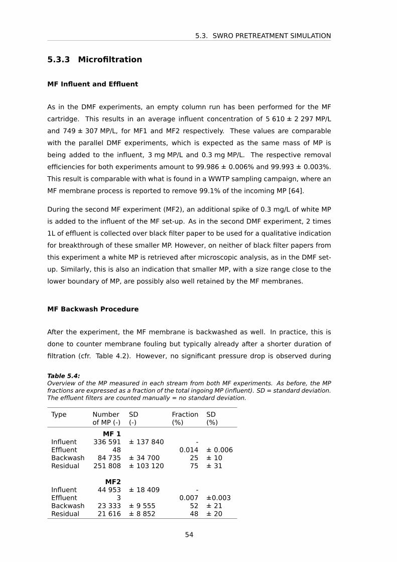
5.3. SWRO PRETREATMENT SIMULATION
5.3.3 Microfiltration
MF Influent and Effluent
As in the DMF experiments, an empty column run has been performed for the MF
cartridge. This results in an average influent concentration of 5 610 ± 2 297 MP/L
and 749 ± 307 MP/L, for MF1 and MF2 respectively. These values are comparable
with the parallel DMF experiments, which is expected as the same mass of MP is
being added to the influent, 3 mg MP/L and 0.3 mg MP/L. The respective removal
efficiencies for both experiments amount to 99.986 ± 0.006% and 99.993 ± 0.003%.
This result is comparable with what is found in a WWTP sampling campaign, where an
MF membrane process is reported to remove 99.1% of the incoming MP [64].
During the second MF experiment (MF2), an additional spike of 0.3 mg/L of white MP
is added to the influent of the MF set-up. As in the second DMF experiment, 2 times
1L of effluent is collected over black filter paper to be used for a qualitative indication
for breakthrough of these smaller MP. However, on neither of black filter papers from
this experiment a white MP is retrieved after microscopic analysis, as in the DMF set-
up. Similarly, this is also an indication that smaller MP, with a size range close to the
lower boundary of MP, are possibly also well retained by the MF membranes.
MF Backwash Procedure
After the experiment, the MF membrane is backwashed as well. In practice, this is
done to counter membrane fouling but typically already after a shorter duration of
filtration (cfr. Table 4.2). However, no significant pressure drop is observed during
Table 5.4:Overview of the MP measured in each stream from both MF experiments. As before, the MPfractions are expressed as a fraction of the total ingoing MP (influent). SD = standard deviation.The effluent filters are counted manually = no standard deviation.
Type Number SD Fraction SDof MP (-) (-) (%) (%)
MF 1Influent 336 591 ± 137 840 -Effluent 48 0.014 ± 0.006Backwash 84 735 ± 34 700 25 ± 10Residual 251 808 ± 103 120 75 ± 31
MF2Influent 44 953 ± 18 409 -Effluent 3 0.007 ±0.003Backwash 23 333 ± 9 555 52 ± 21Residual 21 616 ± 8 852 48 ± 20
54
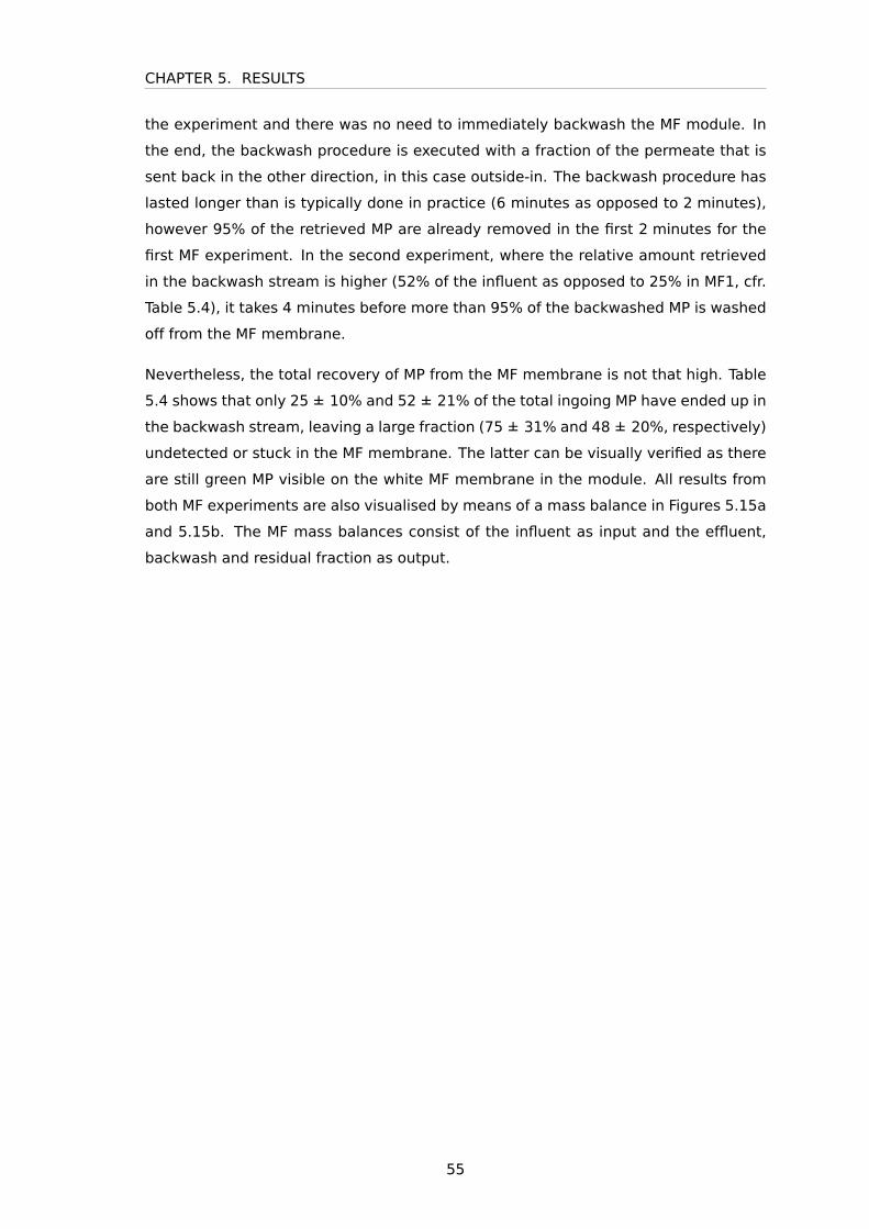
CHAPTER 5. RESULTS
the experiment and there was no need to immediately backwash the MF module. In
the end, the backwash procedure is executed with a fraction of the permeate that is
sent back in the other direction, in this case outside-in. The backwash procedure has
lasted longer than is typically done in practice (6 minutes as opposed to 2 minutes),
however 95% of the retrieved MP are already removed in the first 2 minutes for the
first MF experiment. In the second experiment, where the relative amount retrieved
in the backwash stream is higher (52% of the influent as opposed to 25% in MF1, cfr.
Table 5.4), it takes 4 minutes before more than 95% of the backwashed MP is washed
off from the MF membrane.
Nevertheless, the total recovery of MP from the MF membrane is not that high. Table
5.4 shows that only 25 ± 10% and 52 ± 21% of the total ingoing MP have ended up in
the backwash stream, leaving a large fraction (75 ± 31% and 48 ± 20%, respectively)
undetected or stuck in the MF membrane. The latter can be visually verified as there
are still green MP visible on the white MF membrane in the module. All results from
both MF experiments are also visualised by means of a mass balance in Figures 5.15a
and 5.15b. The MF mass balances consist of the influent as input and the effluent,
backwash and residual fraction as output.
55
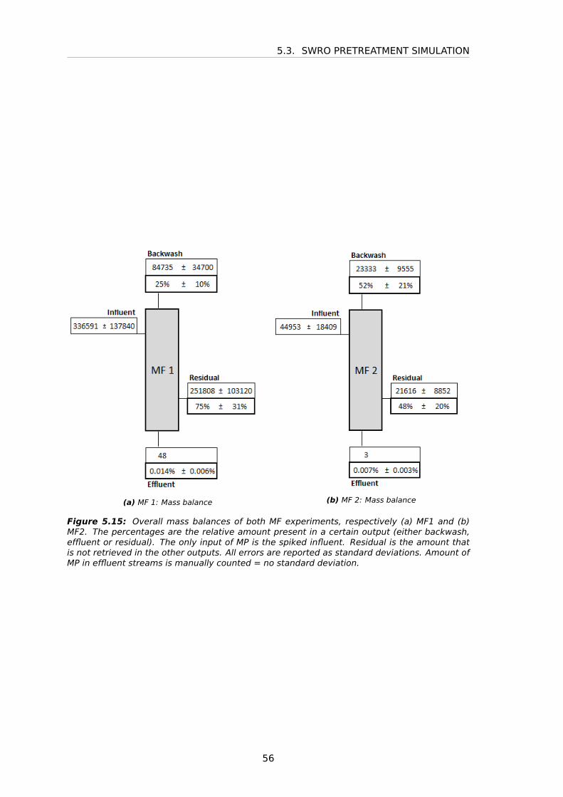
5.3. SWRO PRETREATMENT SIMULATION
(a) MF 1: Mass balance (b) MF 2: Mass balance
Figure 5.15: Overall mass balances of both MF experiments, respectively (a) MF1 and (b)MF2. The percentages are the relative amount present in a certain output (either backwash,effluent or residual). The only input of MP is the spiked influent. Residual is the amount thatis not retrieved in the other outputs. All errors are reported as standard deviations. Amount ofMP in effluent streams is manually counted = no standard deviation.
56
CHAPTER 6
PLASTIC FLUX SIMULATION
6.1 Plastic Flux
In the final part of this research, a desktop study is performed to estimate the amount
of MP that may pass through a full-scale SWRO installation. At first, a preliminary es-
timation is worked out to get an idea of the orders of magnitude of the sketched
situation. Secondly, based on this estimation and also using the results from the
experimental part of this research, various scenarios are studied by making mass bal-
ances over a general SWRO installation to predict the hotspots where incoming MP
are separated and in which streams they end up. For estimation purposes, character-
istics from the earlier described large-scale plant (Ashkelon (Israel), cfr. Table 2.2) are
used.
The first calculations consider the total plastic flux through an SWRO system, regard-
less of separation steps and efficiencies. The MP concentration is derived from liter-
ature. As described in Section 2.1.2, the studies mentioned in Li et al. [6] that use a
fine sampling method (down to 50 µm) and are performed in coastal areas, where the
intake system of an SWRO installations is also located, report MP concentrations in
the order of magnitude of 1 000 to 10 000 MP/m3 [20,21]. Therefore, a concentration
of 1 MP/L (1 000 MP/m3) is selected. This assumption is also supported by the expert
knowledge of Prof. Dr. Colin Janssen (University of Ghent). It is obvious that exact
concentrations are hard to pin down and that such estimations are subject to a high
degree of uncertainty. Therefore this estimation is in the first place presented as an
attempt to create a first idea of the order of magnitude of the studied phenomenon.
Further assumptions include: 100% of the MP entering the water intake system of
the SWRO installation pass through the entire installation; the average mass of an MP
particle is set at 0.005 mg/item, which was also derived as an average from reported
findings of MP in natural samples [6,11,19]. The plastic particle flux is then calculated
using:
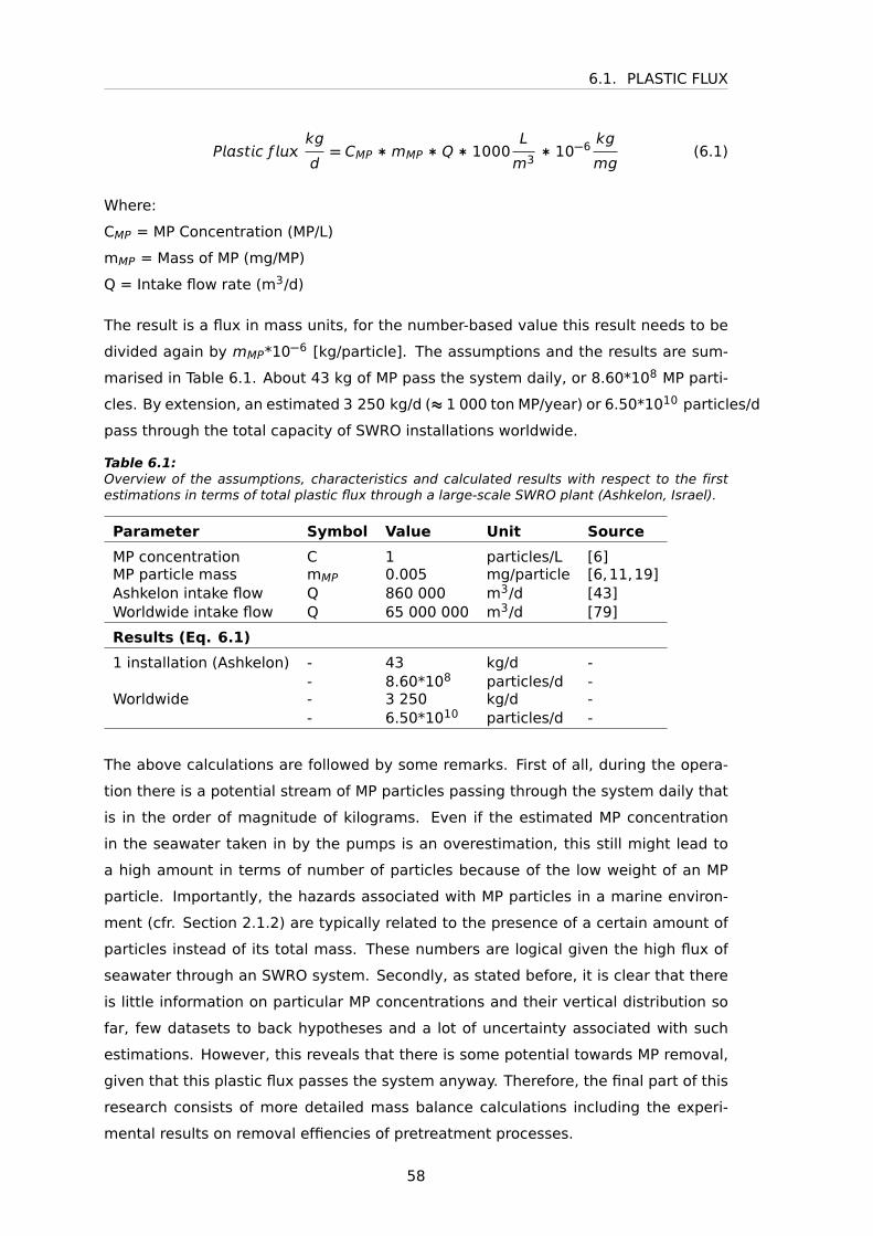
6.1. PLASTIC FLUX
Pstc ƒ kg
d= CMP ∗mMP ∗Q∗ 1000
L
m3∗ 10−6
kg
mg(6.1)
Where:
CMP = MP Concentration (MP/L)
mMP = Mass of MP (mg/MP)
Q = Intake flow rate (m3/d)
The result is a flux in mass units, for the number-based value this result needs to be
divided again by mMP*10−6 [kg/particle]. The assumptions and the results are sum-
marised in Table 6.1. About 43 kg of MP pass the system daily, or 8.60*108 MP parti-
cles. By extension, an estimated 3 250 kg/d (≈ 1 000 ton MP/year) or 6.50*1010 particles/d
pass through the total capacity of SWRO installations worldwide.
Table 6.1:Overview of the assumptions, characteristics and calculated results with respect to the firstestimations in terms of total plastic flux through a large-scale SWRO plant (Ashkelon, Israel).
Parameter Symbol Value Unit Source
MP concentration C 1 particles/L [6]MP particle mass mMP 0.005 mg/particle [6,11,19]Ashkelon intake flow Q 860 000 m3/d [43]Worldwide intake flow Q 65 000 000 m3/d [79]
Results (Eq. 6.1)
1 installation (Ashkelon) - 43 kg/d -- 8.60*108 particles/d -
Worldwide - 3 250 kg/d -- 6.50*1010 particles/d -
The above calculations are followed by some remarks. First of all, during the opera-
tion there is a potential stream of MP particles passing through the system daily that
is in the order of magnitude of kilograms. Even if the estimated MP concentration
in the seawater taken in by the pumps is an overestimation, this still might lead to
a high amount in terms of number of particles because of the low weight of an MP
particle. Importantly, the hazards associated with MP particles in a marine environ-
ment (cfr. Section 2.1.2) are typically related to the presence of a certain amount of
particles instead of its total mass. These numbers are logical given the high flux of
seawater through an SWRO system. Secondly, as stated before, it is clear that there
is little information on particular MP concentrations and their vertical distribution so
far, few datasets to back hypotheses and a lot of uncertainty associated with such
estimations. However, this reveals that there is some potential towards MP removal,
given that this plastic flux passes the system anyway. Therefore, the final part of this
research consists of more detailed mass balance calculations including the experi-
mental results on removal effiencies of pretreatment processes.
58
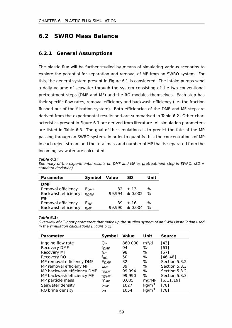
CHAPTER 6. PLASTIC FLUX SIMULATION
6.2 SWRO Mass Balance
6.2.1 General Assumptions
The plastic flux will be further studied by means of simulating various scenarios to
explore the potential for separation and removal of MP from an SWRO system. For
this, the general system present in Figure 6.1 is considered. The intake pumps send
a daily volume of seawater through the system consisting of the two conventional
pretreatment steps (DMF and MF) and the RO modules themselves. Each step has
their specific flow rates, removal efficiency and backwash efficiency (i.e. the fraction
flushed out of the filtration system). Both efficiencies of the DMF and MF step are
derived from the experimental results and are summarised in Table 6.2. Other char-
acteristics present in Figure 6.1 are derived from literature. All simulation parameters
are listed in Table 6.3. The goal of the simulations is to predict the fate of the MP
passing through an SWRO system. In order to quantify this, the concentrations of MP
in each reject stream and the total mass and number of MP that is separated from the
incoming seawater are calculated.
Table 6.2:Summary of the experimental results on DMF and MF as pretreatment step in SWRO. (SD =standard deviation)
Parameter Symbol Value SD Unit
DMFRemoval efficiency EDMF 32 ± 13 %Backwash efficiency ηDMF 99.994 ± 0.002 %MFRemoval efficiency EMF 39 ± 16 %Backwash efficiency ηMF 99.990 ± 0.004 %
Table 6.3:Overview of all input parameters that make up the studied system of an SWRO installation usedin the simulation calculations (Figure 6.1).
Parameter Symbol Value Unit Source
Ingoing flow rate Qn 860 000 m3/d [43]Recovery DMF fDMF 94 % [61]Recovery MF fMF 98 % [57]Recovery RO fRO 50 % [46–48]MP removal efficiency DMF EDMF 32 % Section 5.3.2MP removal efficieny MF EMF 39 % Section 5.3.3MP backwash efficiency DMF ηDMF 99.994 % Section 5.3.2MP backwash efficiency MF ηDMF 99.990 % Section 5.3.3MP particle mass mMP 0.005 mg/MP [6,11,19]Seawater density ρSW 1027 kg/m3 [78]RO brine density ρB 1054 kg/m3 [78]
59
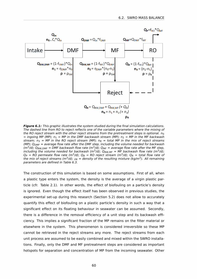
6.2. SWRO MASS BALANCE
Figure 6.1: This graphic illustrates the system studied during the final simulation calculations.The dashed line from RO to reject reflects one of the variable parameters where the mixing ofthe RO reject stream with the other reject streams from the pretreatment steps is optional. n0= ingoing MP (MP); n1 = MP in the DMF backwash stream (MP); n2 = MP in the MF backwashstream; n3 = MP in the RO reject stream (MP); nR = total MP in the mix of reject streams(MP); QDMF = average flow rate after the DMF step, including the volume needed for backwash(m3/d); QBW,DMF = DMF backwash flow rate (m3/d); QMF = average flow rate after the MF step,including the volume needed for backwash (m3/d); QBW,MF = MF backwash flow rate (m3/d);QP = RO permeate flow rate (m3/d); QB = RO reject stream (m3/d); QR = total flow rate ofthe mix of reject streams (m3/d); ρR = density of the resulting mixture (kg/m3). All remainingparameters are defined in Table 6.3.
The construction of this simulation is based on some assumptions. First of all, when
a plastic type enters the system, the density is the average of a virgin plastic par-
ticle (cfr. Table 2.1). In other words, the effect of biofouling on a particle’s density
is ignored. Even though the effect itself has been observed in previous studies, the
experimental set-up during this research (Section 5.2) does not allow to accurately
quantify this effect of biofouling on a plastic particle’s density in such a way that a
significant effect on its floating behaviour in seawater can be assumed. Secondly,
there is a difference in the removal efficiency of a unit step and its backwash effi-
ciency. This implies a significant fraction of the MP remains on the filter material or
elsewhere in the system. This phenomenon is considered irreversible so these MP
cannot be retrieved in the reject streams any more. The reject streams from each
unit process are assumed to be easily combined and mixed within the SWRO installa-
tions. Finally, only the DMF and MF pretreatment steps are considered as important
hotspots for separation and concentration of MP from the incoming seawater. Other
60
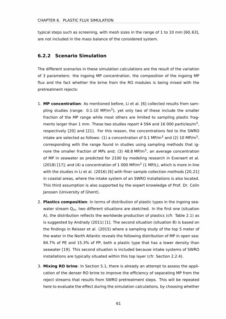
CHAPTER 6. PLASTIC FLUX SIMULATION
typical steps such as screening, with mesh sizes in the range of 1 to 10 mm [60,63],
are not included in the mass balance of the considered system.
6.2.2 Scenario Simulation
The different scenarios in these simulation calculations are the result of the variation
of 3 parameters: the ingoing MP concentration, the composition of the ingoing MP
flux and the fact whether the brine from the RO modules is being mixed with the
pretreatment rejects:
1. MP concentration: As mentioned before, Li et al. [6] collected results from sam-
pling studies (range: 0.1-10 MP/m3), yet only two of these include the smaller
fraction of the MP range while most others are limited to sampling plastic frag-
ments larger than 1 mm. These two studies report 4 594 and 16 000 particles/m3,
respectively [20] and [21]. For this reason, the concentrations fed to the SWRO
intake are selected as follows: (1) a concentration of 0.1 MP/m3 and (2) 10 MP/m3,
corresponding with the range found in studies using sampling methods that ig-
nore the smaller fraction of MPs and; (3) 48.8 MP/m3, an average concentration
of MP in seawater as predicted for 2100 by modeling research in Everaert et al.
(2018) [17]; and (4) a concentration of 1 000 MP/m3 (1 MP/L), which is more in line
with the studies in Li et al. (2016) [6] with finer sample collection methods [20,21]
in coastal areas, where the intake system of an SWRO installations is also located.
This third assumption is also supported by the expert knowledge of Prof. Dr. Colin
Janssen (University of Ghent).
2. Plastics composition: In terms of distribution of plastic types in the ingoing sea-
water stream Qn, two different situations are sketched. In the first one (situation
A), the distribution reflects the worldwide production of plastics (cfr. Table 2.1) as
is suggested by Andrady (2011) [1]. The second situation (situation B) is based on
the findings in Reisser et al. (2015) where a sampling study of the top 5 meter of
the water in the North Atlantic reveals the following distribution of MP in open sea:
84.7% of PE and 15.3% of PP, both a plastic type that has a lower density than
seawater [19]. This second situation is included because intake systems of SWRO
installations are typically situated within this top layer (cfr. Section 2.2.4).
3. Mixing RO brine: In Section 5.1, there is already an attempt to assess the appli-
cation of the denser RO brine to improve the efficiency of separating MP from the
reject streams that results from SWRO pretreatment steps. This will be repeated
here to evaluate the effect during the simulation calculations, by choosing whether
61
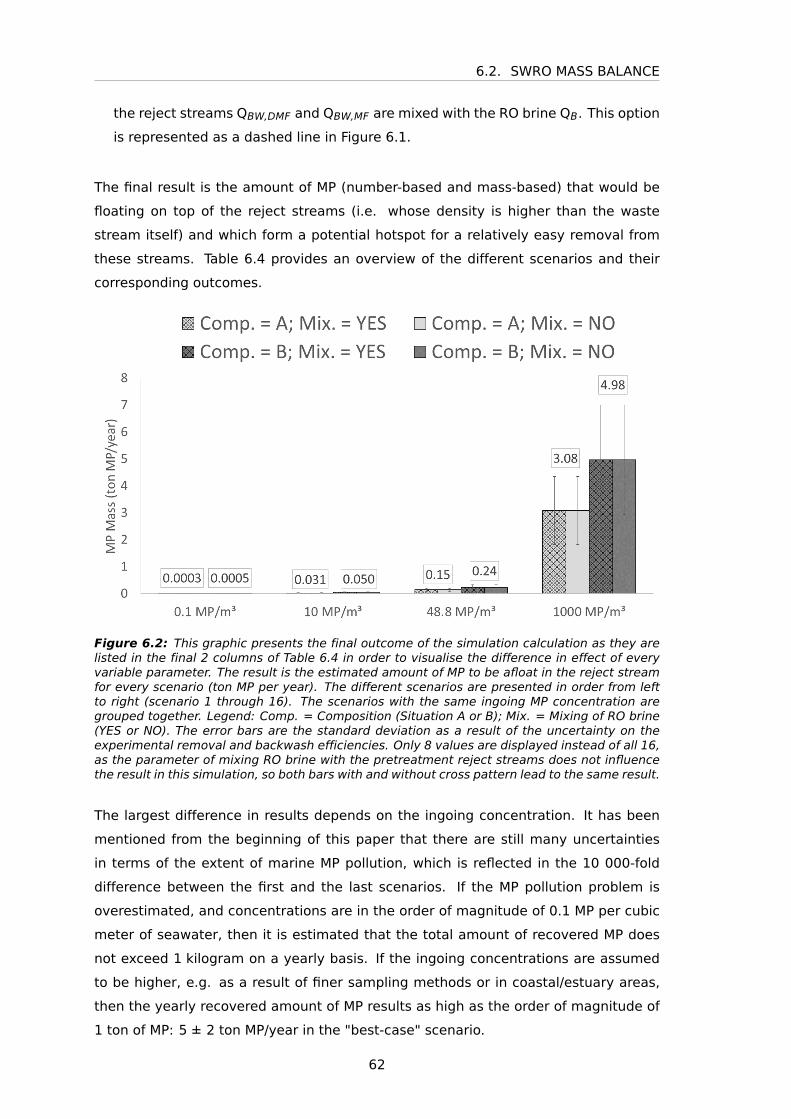
6.2. SWRO MASS BALANCE
the reject streams QBW,DMF and QBW,MF are mixed with the RO brine QB. This option
is represented as a dashed line in Figure 6.1.
The final result is the amount of MP (number-based and mass-based) that would be
floating on top of the reject streams (i.e. whose density is higher than the waste
stream itself) and which form a potential hotspot for a relatively easy removal from
these streams. Table 6.4 provides an overview of the different scenarios and their
corresponding outcomes.
Figure 6.2: This graphic presents the final outcome of the simulation calculation as they arelisted in the final 2 columns of Table 6.4 in order to visualise the difference in effect of everyvariable parameter. The result is the estimated amount of MP to be afloat in the reject streamfor every scenario (ton MP per year). The different scenarios are presented in order from leftto right (scenario 1 through 16). The scenarios with the same ingoing MP concentration aregrouped together. Legend: Comp. = Composition (Situation A or B); Mix. = Mixing of RO brine(YES or NO). The error bars are the standard deviation as a result of the uncertainty on theexperimental removal and backwash efficiencies. Only 8 values are displayed instead of all 16,as the parameter of mixing RO brine with the pretreatment reject streams does not influencethe result in this simulation, so both bars with and without cross pattern lead to the same result.
The largest difference in results depends on the ingoing concentration. It has been
mentioned from the beginning of this paper that there are still many uncertainties
in terms of the extent of marine MP pollution, which is reflected in the 10 000-fold
difference between the first and the last scenarios. If the MP pollution problem is
overestimated, and concentrations are in the order of magnitude of 0.1 MP per cubic
meter of seawater, then it is estimated that the total amount of recovered MP does
not exceed 1 kilogram on a yearly basis. If the ingoing concentrations are assumed
to be higher, e.g. as a result of finer sampling methods or in coastal/estuary areas,
then the yearly recovered amount of MP results as high as the order of magnitude of
1 ton of MP: 5 ± 2 ton MP/year in the "best-case" scenario.
62
CHAPTER 6. PLASTIC FLUX SIMULATION
The 2 situations in terms of plastic composition (situations A or B) determine the
eventually recovered (i.e. by density separation) fraction of the MP that end up in
the final waste stream. In situation A, about 62% of the incoming plastic is lighter
than seawater while in situation B, based on an analysis of sampled MP in the upper
5 meter layer, all plastic types that occur are lighter than seawater.
The final parameter is the mixing of RO brine with the other reject streams in order
to increase the density of the reject mixture for more efficient density separation.
However, it turns out that for the given incoming MP streams, there is no effect of this
parameter on the result in any scenario.
63
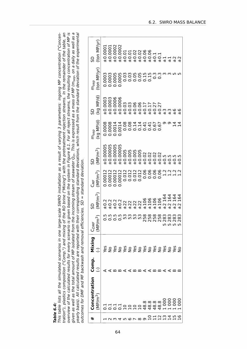
6.2. SWRO MASS BALANCE
Table
6.4:
This
table
lists
all
the
sim
ula
ted
scen
ario
sin
one
larg
e-sc
ale
SW
RO
inst
alla
tion
asa
resu
ltof
vary
ing
3par
amet
ers:
ingoi
ng
MP
conce
ntr
atio
n("
Con
cen-
trat
ion")
,pla
stic
sco
mpos
itio
n("
Com
p."
)an
dm
ixin
gof
the
RO
bri
ne
("M
ixin
g")
wit
hth
epre
trea
tmen
tre
ject
ion
stre
ams.
Inth
ere
mai
nder
ofth
eta
ble
,an
over
view
ofth
eca
lcula
ted
resu
lts
for
ever
ysc
enar
iois
giv
enbas
edon
the
syst
emin
Figure
6.1
.Fo
ral
lrej
ect
stre
ams,
the
resu
ltin
gco
nce
ntr
atio
nof
MP
isgiv
enas
wel
las
the
tota
lam
ount
ofM
Pis
olat
edfr
omth
ein
com
ing
stre
amof
seaw
ater
Qn
.Th
isis
expre
ssed
asa
mas
sof
MP
(msep,
ona
dai
lyas
wel
las
aye
arly
bas
is).
All
calc
ula
ted
resu
lts
are
repor
ted
wit
hth
eir
corr
espon
din
gst
andar
ddev
iati
ons,
whic
hre
sult
from
the
stan
dar
ddev
iati
onof
the
exper
imen
tal
outc
omes
for
DM
Fan
dM
Fbac
kwas
han
dre
mov
alef
fici
enci
es.
SD
=st
andar
ddev
iati
on.
#C
on
cen
trati
on
Com
p.
Mix
ing
CDMF
SD
CMF
SD
msep
SD
msep
SD
(MP/
m3)
(-)
(-)
(MP/
m3)
(MP/
m3)
(MP/
m3)
(MP/
m3)
(kg
MP/
d)
(kg
MP/
d)
(ton
MP/
yr)
(ton
MP/
yr)
10
.1A
Yes
0.5±
0.2
0.0
00
12±
0.0
00
05
0.0
00
8±
0.0
00
30
.00
03
±0
.00
01
20
.1A
No
0.5±
0.2
0.0
00
12±
0.0
00
05
0.0
00
8±
0.0
00
30
.00
03
±0
.00
01
30
.1B
Yes
0.5±
0.2
0.0
00
12±
0.0
00
05
0.0
01
4±
0.0
00
60
.00
05
±0
.00
02
40
.1B
No
0.5±
0.2
0.0
00
12±
0.0
00
05
0.0
01
4±
0.0
00
60
.00
05
±0
.00
02
51
0A
Yes
53±
22
0.0
12±
0.0
05
0.0
8±
0.0
30
.03
±0
.01
61
0A
No
53±
22
0.0
12±
0.0
05
0.0
8±
0.0
30
.03
±0
.01
71
0B
Yes
53±
22
0.0
12±
0.0
05
0.1
4±
0.0
60
.05
±0
.02
81
0B
No
53±
22
0.0
12±
0.0
05
0.1
4±
0.0
60
.05
±0
.02
94
8.8
AYe
s2
58±
10
60
.06±
0.0
20
.41±
0.1
70
.15
±0
.06
10
48
.8A
No
25
8±
10
60
.06±
0.0
20
.41±
0.1
70
.15
±0
.06
11
48
.8B
Yes
25
8±
10
60
.06±
0.0
20
.67±
0.2
70
.3±
0.1
12
48
.8B
No
25
8±
10
60
.06±
0.0
20
.67±
0.2
70
.3±
0.1
13
10
00
AYe
s5
28
3±
21
64
1.2±
0.5
9±
33
±1
14
10
00
AN
o5
28
3±
21
64
1.2±
0.5
9±
33
±1
15
10
00
BYe
s5
28
3±
21
64
1.2±
0.5
14±
65
±2
16
10
00
BN
o5
28
3±
21
64
1.2±
0.5
14±
65
±2
64
CHAPTER 7
DISCUSSION
7.1 Experimental research
The first part of the experimental research focusses on the influence of biofouling on
the density of a plastic particle. First of all, the method to determine the density is
not accurate enough to follow up the progress of the particles’ density through time.
All experiments on PE beads (both Biofouling 1 and Biofouling 2, with different condi-
tions) do not reveal a correlation between biofilm formation (measured by means of
ATP concentration) and the particle density. The only experiment which gives an indi-
cation of this correlation between both, which has been observed before in previous
research, is the one experiment on PP particles. This can be explained by the differ-
ence in density of the virgin plastic beads: the PE beads have a density of 0.98 g/cm3,
the PP beads only 0.90 g/cm3. Because of this, the absolute difference between plas-
tic density and biofilm density (1.14 g/cm3, cfr. Section 2.1.3) is larger for the PP
beads and an effect (i.e. an increase of density due to a higher degree of biofouling,
as reflected in an increase in ATP concentration) can be observed more easily than
for the heavier PE beads, whose density is closer to the biofilm’s density.
The second part of the experimental research assesses the fate of MP in SWRO pre-
treatment processes. Table 6.2 summarises the removal and backwash efficiencies
from the experimental set-ups for DMF and MF. Firstly, it is shown that both pretreat-
ment steps are very efficient in terms of removal of MP from the incoming (sea)water
stream, both for PE in the size range of 90-106 µm (quantitatively) and of 10-45 µm
(qualitatively). MP present in the incoming seawater of an SWRO installation do not
reach the RO modules itself. Instead, they are held up in the pretreatment process.
Also, the analysis of the vertical distribution of MP in the DMF columns show no sign
of breakthrough: over 90% of the MP present in the filter material is retrieved in
the top 2 segments (out of 10 = top 20% of the column). Lastly, both DMF and MF
were executed in a first series with tap water (DMF1 and MF1). Later they were per-
formed with seawater (DMF2 and MF2) to better simulate a realistic SWRO scenario
(cfr. Table 4.3). However, given the uncertainty on the measurements resulting from
7.2. SIMULATIONS
these experiments, a difference in outcomes cannot be stated between both types of
feed water.
The goal of this thesis research is to point out hotspots where MP are concentrated
throughout the system in order to form a basis for further research on methods to
remove MP from these concentrated reject streams. In this study, the resulting back-
wash efficiencies allow to further trace the MP in the described system as they end
up in the reject streams of the two studied pretreatment steps. The two studied set-
ups result in backwash efficiencies of 32% and 39%, for DMF and MF respectively.
The DMF pretreatment step typically precedes the MF step and it is shown that a
DMF step has a high removal efficiency of MP, so only a very small fraction of the
incoming MP will reach as far as the MF units. As a consequence, the majority of the
recovered MP will be found in the DMF reject stream. In practice, this reject stream
is typically discharged again in the sea or the ocean from where the original intake
water is drawn.
7.2 Simulations
The simulation calculations indicate a broad range of results in terms of removal po-
tential of MP in this way. On the one hand, there are the most conservative scenarios
in which only a fraction floats on top of the reject streams and the concentrations are
low: 0.1 to 10 MP/m3. These concentrations are typically the result of sampling stud-
ies in open sea. Based on these conservative parameters, the removal of potential
of MP in this process is estimated to range from 0.3 kg to 50 kg per year, for one
large-scale SWRO installation. On the other hand, when incoming MP concentrations
are higher, as they are reported in coastal and estuary areas or as they are estimated
to increase in the future, this potential is estimated to range from 150 kg to as high as
5 tonnes of MP per year, for one large-scale SWRO installation. In terms of MP, this is
a very significant amount that can potentially be removed from sea water in existing
installations. In order to put these results in some context, the worldwide production
of plastics exceeds 300 million tonnes/year (cfr. Figure 2.1). Eriksen et al. (2014) [22]
report an estimate of the worldwide MP pollution: 268 940 tonnes or 5.25 trillion plas-
tic particles. Andrady (2017) [3] estimates a yearly input of 4.8-12.7 million tonnes
of waste plastics ending up as litter in the oceans. These numbers vary strongly but
the order of magnitude is clearly higher than what is calculated in this study in terms
of removal. However, as a flux of plastic particle passes through such large-scale
installations either way, these findings indicate the potential to remove a fraction of
the MP pollution, albeit a small one.
66
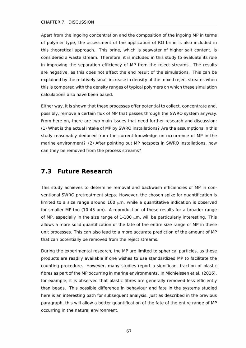
CHAPTER 7. DISCUSSION
Apart from the ingoing concentration and the composition of the ingoing MP in terms
of polymer type, the assessment of the application of RO brine is also included in
this theoretical approach. This brine, which is seawater of higher salt content, is
considered a waste stream. Therefore, it is included in this study to evaluate its role
in improving the separation efficiency of MP from the reject streams. The results
are negative, as this does not affect the end result of the simulations. This can be
explained by the relatively small increase in density of the mixed reject streams when
this is compared with the density ranges of typical polymers on which these simulation
calculations also have been based.
Either way, it is shown that these processes offer potential to collect, concentrate and,
possibly, remove a certain flux of MP that passes through the SWRO system anyway.
From here on, there are two main issues that need further research and discussion:
(1) What is the actual intake of MP by SWRO installations? Are the assumptions in this
study reasonably deduced from the current knowledge on occurrence of MP in the
marine environment? (2) After pointing out MP hotspots in SWRO installations, how
can they be removed from the process streams?
7.3 Future Research
This study achieves to determine removal and backwash efficiencies of MP in con-
ventional SWRO pretreatment steps. However, the chosen spike for quantification is
limited to a size range around 100 µm, while a quantitative indication is observed
for smaller MP too (10-45 µm). A reproduction of these results for a broader range
of MP, especially in the size range of 1-100 µm, will be particularly interesting. This
allows a more solid quantification of the fate of the entire size range of MP in these
unit processes. This can also lead to a more accurate prediction of the amount of MP
that can potentially be removed from the reject streams.
During the experimental research, the MP are limited to spherical particles, as these
products are readily available if one wishes to use standardized MP to facilitate the
counting procedure. However, many studies report a significant fraction of plastic
fibres as part of the MP occurring in marine environments. In Michielssen et al. (2016),
for example, it is observed that plastic fibres are generally removed less efficiently
than beads. This possible difference in behaviour and fate in the systems studied
here is an interesting path for subsequent analysis. Just as described in the previous
paragraph, this will allow a better quantification of the fate of the entire range of MP
occurring in the natural environment.
67
7.3. FUTURE RESEARCH
Finally, in the simulation calculations, two variable parameters strongly influenced
the end result. Both parameters have been selected to vary as there is little certainty
about their true nature. The ingoing concentration and the composition of the plastic
flux is crucial in making a better prediction of the total amount of MP that enters an
SWRO installation and the total amount of ’end product’, i.e. the recovered mass of
MP. Especially knowledge on the vertical distribution of MP in the top layer of the water
mass is crucial in estimating the order of magnitude of the plastic flux through SWRO
installations. Are the ingoing MP predominantly PE and PP? Can their concentration
at a certain depth be predicted by sampling at the surface? In relation to this, exper-
imental studies to more accurately quantify the rate of biofouling and, subsequently,
the rate of density change of a certain plastic particle are an interesting addition to
the story of MP marine pollution. The type of MP and their density, once they end up
in the indicated reject streams, are an important characteristic to further study their
removal potential: what technologies are available and how can they be implemented
in a reasonable way?
68
CHAPTER 8
CONCLUSION
MP pollution of the marine environment is a widespread and globally observed phe-
nomenon. SWRO installations process high flow rates of seawater (up to the order of
magnitude of 100 000 m3/d) for the production of drinking water. At the same time,
MP that are present in this processed seawater pass through the same pretreatment
steps as the seawater. This study has investigated the fate of MP during these steps:
both DMF and MF retain over 99.9% of the incoming MP in the bench-scale set-ups.
At the same time, respectively 32% and 39% of the ingoing flux is washed out again
during the backwash procedures. In this way, a fraction of the MP taken in by such in-
stallations eventually ends up in a reject stream of the DMF pretreatment step which
is of lower total volume than the original polluted seawater and, consequently, of a
higher concentration of MP.
These findings reveal a potential for removal of this plastic flux from the SWRO pro-
cess. The most conservative approach results in about 6·108 plastic particles (0.3
kg MP/year), while more optimistic scenarios result in up to 1·1013 plastic particles
(5 tonnes MP/year). Further research is challenged to investigate in which way this
separation can take place: density separation, e.g. settling or centrifugation, or size
separation, e.g. additional membrane filtration. The central question is how such a
technology can be implemented within the existing systems in a reasonable and eco-
nomical way, given the fact that there is no obvious (economical) production value.
The concentration of MP in the reject streams, due to the normal operation of an
SWRO installation, is one step. The next step is to remove this flux of MP in an effec-
tive way but with minimal additional costs for the operator.
If further research is able to pinpoint cost-effective and easily implemented technol-
ogy to remove this MP flux before it is sent back into the marine environment, as is the
case in conventional operation, this may offer an interesting pathway to remedy part
of the MP pollution problem and produce an added value to the operation of SWRO
installations in ecological terms.

70
BIBLIOGRAPHY
[1] A. L. Andrady, “Microplastics in the marine environment,” Marine Pollution Bul-
letin, vol. 62, no. 8, pp. 1596–1605, 2011.
[2] L. G. A. Barboza and B. C. G. Gimenez, “Microplastics in the marine environment:
Current trends and future perspectives,” Marine Pollution Bulletin, vol. 97, no. 1-
2, pp. 5–12, 2015.
[3] A. L. Andrady, “The plastic in microplastics: A review,” Marine Pollution Bulletin,
vol. 119, no. 1, pp. 12–22, 2017.
[4] C. Stevens, Polymeren: course notes. 2015.
[5] R. Geyer, J. R. Jambeck, and K. L. Law, “Production, use, and fate of all plastics
ever made,” Science Advances, vol. 3, no. 7, 2017.
[6] W. C. Li, H. F. Tse, and L. Fok, “Plastic waste in the marine environment: A review
of sources, occurrence and effects,” Science of the Total Environment, vol. 566-
567, pp. 333–349, 2016.
[7] J. G. B. Derraik, “The pollution of the marine environment by plastic debris: a
review.,” Marine Pollution Bulletin, vol. 44, pp. 842–852, 2002.
[8] J. Lee, S. Hong, Y. K. Song, S. H. Hong, Y. C. Jang, M. Jang, N. W. Heo, G. M.
Han, M. J. Lee, D. Kang, and W. Shim, “Relationships among the abundances
of plastic debris in different size classes on beaches in South Korea,” Marine
Pollution Bulletin, vol. 77, no. 1-2, pp. 349–354, 2013.
[9] R. C. Thompson, “Plastic debris in the marine environment: consequences and
solutions,” Marine Nature Conservation in Europe, pp. 107–116, May 2006.
[10] UNEP, “Marine plastic debris and microplastics - Global lessons and research to
inspire action and guide policy change.,” United Nations Environment Program,
Nairobi, 2016.
[11] C. G. Avio, S. Gorbi, and F. Regoli, “Plastics and microplastics in the oceans:
From emerging pollutants to emerged threat,” Marine Environmental Research,
vol. 128, pp. 2–11, 2017.
BIBLIOGRAPHY
[12] H. S. Auta, C. U. Emenike, and S. H. Fauziah, “Distribution and importance of
microplastics in the marine environment: A review of the sources, fate, effects,
and potential solutions,” Environment International, vol. 102, pp. 165–176, 2017.
[13] J. Zhao, W. Ran, J. Teng, Y. Liu, H. Liu, X. Yin, R. Cao, and Q. Wang, “Microplastic
pollution in sediments from the Bohai Sea and the Yellow Sea, China,” Science of
the Total Environment, vol. 640-641, pp. 637–645, 2018.
[14] R. C. Thompson, “Lost at Sea: Where Is All the Plastic?,” Science, vol. 304,
no. 5672, p. 838, 2004.
[15] C. M. Free, O. P. Jensen, S. A. Mason, M. Eriksen, N. J. Williamson, and B. Boldgiv,
“High-levels of microplastic pollution in a large, remote, mountain lake,” Marine
Pollution Bulletin, vol. 85, no. 1, pp. 156–163, 2014.
[16] D. Eerkes-Medrano, R. C. Thompson, and D. C. Aldridge, “Microplastics in fresh-
water systems: A review of the emerging threats, identification of knowledge
gaps and prioritisation of research needs,” Water Research, vol. 75, pp. 63–82,
2015.
[17] G. Everaert, L. Van Cauwenberghe, M. De Rijcke, A. A. Koelmans, J. Mees, M. Van-
degehuchte, and C. R. Janssen, “Risk assessment of microplastics in the ocean:
Modelling approach and first conclusions,” Environmental Pollution, vol. 242,
pp. 1930–1938, 2018.
[18] A. Cozar, F. Echevarria, J. I. Gonzalez-Gordillo, X. Irigoien, B. Ubeda,
S. Hernandez-Leon, A. T. Palma, S. Navarro, J. Garcia-de Lomas, A. Ruiz, M. L.
Fernandez-de Puelles, and C. M. Duarte, “Plastic debris in the open ocean,” Pro-
ceedings of the National Academy of Sciences, vol. 111, no. 28, pp. 10239–
10244, 2014.
[19] J. Reisser, B. Slat, K. Noble, K. Du Plessis, M. Epp, M. Proietti, J. De Sonneville,
T. Becker, and C. Pattiaratchi, “The vertical distribution of buoyant plastics at
sea: An observational study in the North Atlantic Gyre,” Biogeosciences, vol. 12,
no. 4, pp. 1249–1256, 2015.
[20] J.-P. W. Desforges, M. Galbraith, N. Dangerfield, and P. S. Ross, “Widespread dis-
tribution of microplastics in subsurface seawater in the NE Pacific Ocean,” Marine
Pollution Bulletin, vol. 79, no. 1-2, pp. 94–99, 2014.
[21] S. Zhao, L. Zhu, T. Wang, and D. Li, “Suspended microplastics in the surface
water of the Yangtze Estuary System, China : First observations on occurrence,
distribution,” Marine Pollution Bulletin, vol. 86, no. 1-2, pp. 562–568, 2014.
72
BIBLIOGRAPHY
[22] M. Eriksen, L. C. M. Lebreton, H. S. Carson, M. Thiel, C. J. Moore, J. C. Borerro,
F. Galgani, and P. G. Ryan, “Plastic Pollution in the World’ s Oceans: More than
5 Trillion Plastic Pieces Weighing over 250 .000 Tons Afloat at Sea,” PLoS ONE,
vol. 9, no. 12, pp. 1–15, 2014.
[23] A. van Wezel, I. Caris, and S. A. Kools, “Release of primary microplastics from
consumer products to wastewater in the Netherlands,” Environmental Toxicology
and Chemistry, vol. 35, no. 7, pp. 1627–1631, 2016.
[24] H. Lee, H.-J. Lee, and J.-h. Kwon, “Estimating microplastic-bound intake of hy-
drophobic organic chemicals by fish using measured desorption rates to artificial
gut fluid,” Science of the Total Environment, vol. 651, pp. 162–170, 2019.
[25] J. Wang, M. Wang, S. Ru, and X. Liu, “High levels of microplastic pollution in the
sediments and benthic organisms of the South Yellow Sea , China,” Science of
the Total Environment, vol. 651, pp. 1661–1669, 2019.
[26] W. Courtene-Jones, B. Quinn, C. Ewins, S. F. Gary, and B. E. Narayanaswamy,
“Consistent microplastic ingestion by deep-sea invertebrates over the last four
decades (1976-2015 ), a study from the North East Atlantic,” Environmental Pol-
lution, vol. 244, pp. 503–512, 2019.
[27] J. F. Provencher, J. C. Vermaire, S. Avery-gomm, B. M. Braune, and M. L. Mallory,
“Garbage in guano? Microplastic debris found in faecal precursors of seabirds
known to ingest plastics,” Science of the Total Environment, vol. 644, pp. 1477–
1484, 2018.
[28] K. Tanaka, H. Takada, R. Yamashita, K. Mizukawa, and M.-a. Fukuwaka, “Accumu-
lation of plastic-derived chemicals in tissues of seabirds ingesting marine plas-
tics,” Marine Pollution Bulletin, vol. 69, no. 1-2, pp. 219–222, 2013.
[29] E. R. Zettler, T. J. Mincer, and L. A. Amaral-zettler, “Life in the Plastisphere : Mi-
crobial Communities on Plastic Marine Debris,” Environmental Science & Tech-
nology, vol. 47, pp. 7137–7146, 2013.
[30] L. Frère, L. Maignien, M. Chalopin, A. Huvet, E. Rinnert, H. Morrison, S. Kerninon,
A.-l. Cassone, C. Lambert, J. Reveillaud, and I. Paul-Pont, “Microplastic bacterial
communities in the Bay of Brest: Influence of polymer type and size,” Environ-
mental Pollution, vol. 242, pp. 614–625, 2018.
[31] C. D. Rummel, A. Jahnke, E. Gorokhova, D. Kühnel, and M. Schmitt-Jansen, “Im-
pacts of biofilm formation on the fate and potential effects of microplastic in the
aquatic environment,” Environmental Science and Technology Letters, vol. 4,
no. 7, pp. 258–267, 2017.
73
BIBLIOGRAPHY
[32] S. Ye and A. L. Andrady, “Fouling of floating plastic debris under Biscayne Bay
exposure conditions,” Marine Pollution Bulletin, vol. 22, no. 12, pp. 608–613,
1991.
[33] E. A. Pelve, K. M. Fontanez, and E. F. DeLong, “Bacterial succession on sinking
particles in the ocean’s interior,” Frontiers in Microbiology, vol. 8, pp. 1–15, 2017.
[34] United Nations, “Stockholm Convention on Persistent Organic Pollutants (POPs),”
2001.
[35] T. Gouin, N. Roche, R. Lohmann, and G. Hodges, “A Thermodynamic Approach for
Assessing the Environmental Exposure of Chemicals Absorbed to Microplastic,”
Environmental Science and Technology, vol. 45, pp. 1466–1472, 2011.
[36] A. Bakir, S. J. Rowland, and R. C. Thompson, “Enhanced desorption of persistent
organic pollutants from microplastics under simulated physiological conditions,”
Environmental Pollution, vol. 185, pp. 16–23, 2014.
[37] S. W. Hermanowicz and J. J. Ganczarczyk, “Some Fluidization Characteristics of
Biological Beds,” Biotechnology and Bioengineering, vol. 25, no. 5, pp. 1321–
1330, 1983.
[38] M. Kooi, E. H. Van Nes, M. Scheffer, and A. A. Koelmans, “Ups and Downs in the
Ocean: Effects of Biofouling on Vertical Transport of Microplastics,” Environmen-
tal Science and Technology, vol. 51, no. 14, pp. 7963–7971, 2017.
[39] K. L. Law, N. Maximenko, S. Morét-Ferguson, and E. Peacock, “Plastic Accu-
mulation in the North Atlantic Subtropical Gyre,” Science, vol. 329, no. 5996,
pp. 1185–1188, 2010.
[40] L. C. Woodall, A. Sanchez-Vidal, M. Canals, G. L. Paterson, R. Coppock, V. Sleight,
A. Calafat, A. D. Rogers, B. E. Narayanaswamy, and R. C. Thompson, “The deep
sea is a major sink for microplastic debris,” Royal Society Open Science, vol. 1,
no. 4, 2014.
[41] D. Lobelle and M. Cunliffe, “Early microbial biofilm formation on marine plastic
debris,” Marine Pollution Bulletin, vol. 62, no. 1, pp. 197–200, 2011.
[42] F. J. Millero, R. Feistel, D. G. Wright, and T. J. Mcdougall, “The composition of Stan-
dard Seawater and the definition of the Reference-Composition Salinity Scale,”
Deep-Sea Research I, vol. 55, pp. 50–72, 2008.
[43] B. Sauvet-Goichon, “Ashkelon desalination plant: A successful challenge,” De-
salination, vol. 203, pp. 75–81, 2007.
74
BIBLIOGRAPHY
[44] L. F. Greenlee, D. F. Lawler, B. D. Freeman, B. Marrot, P. Moulin, and P. Ce, “Re-
verse osmosis desalination: Water sources, technology, and today’s challenges,”
Water Research, vol. 43, no. 9, pp. 2317–2348, 2009.
[45] GWI, “Market-leading Analysis of the International Water Industry, Global Water
Intelligence,” tech. rep., 2012.
[46] S. S. Shenvi, A. M. Isloor, and A. F. Ismail, “A review on RO membrane technology:
Developments and challenges,” Desalination, vol. 368, pp. 10–26, 2015.
[47] A. R. D. Verliefde, P. Van der Meeren, and B. Van der Bruggen, Solution-Diffusion
Processes, pp. 1–26. 2013.
[48] L. Malaeb and G. M. Ayoub, “Reverse osmosis technology for water treatment:
State of the art review,” Desalination, vol. 267, no. 1, pp. 1–8, 2011.
[49] Water Technology, “Sorek Desalination Plant.” https://www.
water-technology.net/projects/sorek-desalination-plant/, 2019. Ac-
cessed: 2019-03-30.
[50] Hyflux, “Pollution Control Study for Tuas Desalination and Power Plant Project,”
tech. rep., 2011.
[51] Suez, “Al Dur: seawater reverse osmosis desalination plant,” tech. rep., 2019.
[52] M. Lambert, “AlChE Conference 2015,” in AlChE Conference 2015, 2015.
[53] A. Belatoui, H. Bouabessalam, and O. Rouane, “ Environmental effects of
brine discharge from two desalination plants in Algeria (South Western Mediter-
ranean),” Desalination and Water Treatment, vol. 76, no. January, pp. 311–318,
2017.
[54] Suez, “Bahía de Palma: Seawater Reverse Osmosis Desalination Plant Mallorca
(Spain),” tech. rep., 2019.
[55] S. P. Kopko and L. K. Wang, “City of Cape Coral Reverse Osmosis Water Treatment
Facility,” tech. rep., Zorex Corporation, Cape Coral, 2012.
[56] World Bank, “Seawater and Brackish Water Desalination in the Middle East, North
Africa and Central Asia: Final Report - Annex 5 - Malta,” tech. rep., 2004.
[57] S. K. Al-Mashharawi, N. Ghaffour, M. Al-Ghamdi, and G. L. Amy, “Evaluating the
efficiency of different microfiltration and ultrafiltration membranes used as pre-
treatment for Red Sea water reverse osmosis desalination,” Desalination and
Water Treatment, vol. 51, no. 1-3, pp. 617–626, 2013.
75
BIBLIOGRAPHY
[58] A. R. Guastalli, F. X. Simon, Y. Penru, A. D. Kerchove, J. Llorens, and S. Baig,
“Comparison of DMF and UF pre-treatments for particulate material and dis-
solved organic matter removal in SWRO desalination,” Desalination, vol. 322,
pp. 144–150, 2013.
[59] S. Jeong, G. Naidu, R. Vollprecht, T. Leiknes, and S. Vigneswaran, “In-depth anal-
yses of organic matters in a full-scale seawater desalination plant and an au-
topsy of reverse osmosis membrane,” Separation and Purification Technology,
vol. 162, pp. 171–179, 2016.
[60] N. Voutchkov, “Considerations for Selection of Seawater Filtration Pretreatment
System,” Desalination, vol. 261, no. 3, pp. 354–364, 2010.
[61] W. J. Weber, Physicochemical Processes for Water Quality Control. Wiley-
Interscience, illustrate ed., 1972.
[62] N. Sabiri, E. Monnier, V. Raimbault, A. Massé, V. Séchet, and P. Jaouen, “Effect
of filtration rate on coal-sand dual-media filter performances for microalgae re-
moval,” Environmental Technology, vol. 38, no. 3, pp. 345–352, 2017.
[63] S. Jamaly, N. N. Darwish, I. Ahmed, and S. W. Hasan, “A short review on reverse
osmosis pretreatment technologies,” Desalination, vol. 354, pp. 30–38, 2014.
[64] M. R. Michielssen, E. R. Michielssen, J. Ni, and M. B. Duhaime, “Fate of microplas-
tics and other small anthropogenic litter (sal) in wastewater treatment plants
depends on unit processes employed,” Environmental Science: Water Research
& Technology, vol. 2, pp. 1064–1073, 2016.
[65] R. Sutton, S. A. Mason, S. K. Stanek, E. Willis-norton, I. F. Wren, and C. Box,
“Microplastic contamination in the San Francisco Bay, California, USA,” Marine
Pollution Bulletin, vol. 109, no. 1, pp. 230–235, 2016.
[66] L. Yang, K. Li, S. Cui, Y. Kang, L. An, and K. Lei, “Removal of microplastics in mu-
nicipal sewage from China’s largest water reclamation plant,” Water Research,
vol. 155, pp. 175–181, 2019.
[67] E. A. Gies, J. L. LeNoble, M. Noël, A. Etemadifar, F. Bishay, E. R. Hall, and P. S. Ross,
“Retention of microplastics in a major secondary wastewater treatment plant in
Vancouver, Canada,” Marine Pollution Bulletin, vol. 133, no. June, pp. 553–561,
2018.
[68] S. A. Carr, J. Liu, and A. G. Tesoro, “Transport and fate of microplastic particles in
wastewater treatment plants,” Water Research, vol. 91, pp. 174–182, 2016.
76
BIBLIOGRAPHY
[69] T. M. Missimer and R. G. Maliva, “Environmental issues in seawater reverse os-
mosis desalination : Intakes and outfalls,” Desalination, vol. 434, pp. 198–215,
2018.
[70] D. Gille, “Seawater intakes for desalination plants,” Desalination, vol. 156,
pp. 249–256, 2003.
[71] T. Pankratz, “Seawater desalination technology overview,” in Presentation for
Georgia Joint Comprehensive Study Committee, St. Simons Island, Georgia,
2006.
[72] V. Bonnelye, M. A. Sanz, J.-P. Durand, L. Plasse, F. Gueguen, and P. Mazounie, “Re-
verse osmosis on open intake seawater: Pre-treatment strategy,” Desalination,
vol. 167, pp. 191–200, 2004.
[73] M. Ahmed and R. Anwar, “An Assessment of the Environmental Impact of Brine
Disposal in Marine Environment,” International Journal of Modern Engineering
Research, vol. 24, pp. 2756–2761, 2012.
[74] R. Einav and F. Lokiec, “Environmental aspects of a desalination plant in
Ashkelon,” Desalination, vol. 156, pp. 79–85, 2003.
[75] M. Ahmed, D. Hoey, M. R. Thumarukudyd, M. F. A. Goosen, M. Al-haddabi, and
A. Al-belushi, “Feasibility of salt production Corn inland RO desalination plant
reject brine : a case study,” Desalination, vol. 158, pp. 109–117, 2003.
[76] Aqua-Techniek, “Filtermedia for Water Treatment,” tech. rep., 2003.
[77] A. C. Mehner, “Multimedia and Ultrafiltration for Reverse Osmosis Pretreatment
Aboard Naval Vessels,” The University of Arkansas Undergraduate Research Jour-
nal, vol. 11, 2010.
[78] F. J. Millero and F. Huang, “The density of seawater as a function of salinity (5 to
70 g/kg) and temperature (273.15 to 363.15 K),” Ocean Science, vol. 5, pp. 91–
100, 2009.
[79] E. Jones, M. Qadir, M. T. H. V. Vliet, V. Smakhtin, and S.-m. Kang, “The state
of desalination and brine production: A global outlook,” Science of the Total
Environment, vol. 657, pp. 1343–1356, 2019.
77

BIBLIOGRAPHY
78
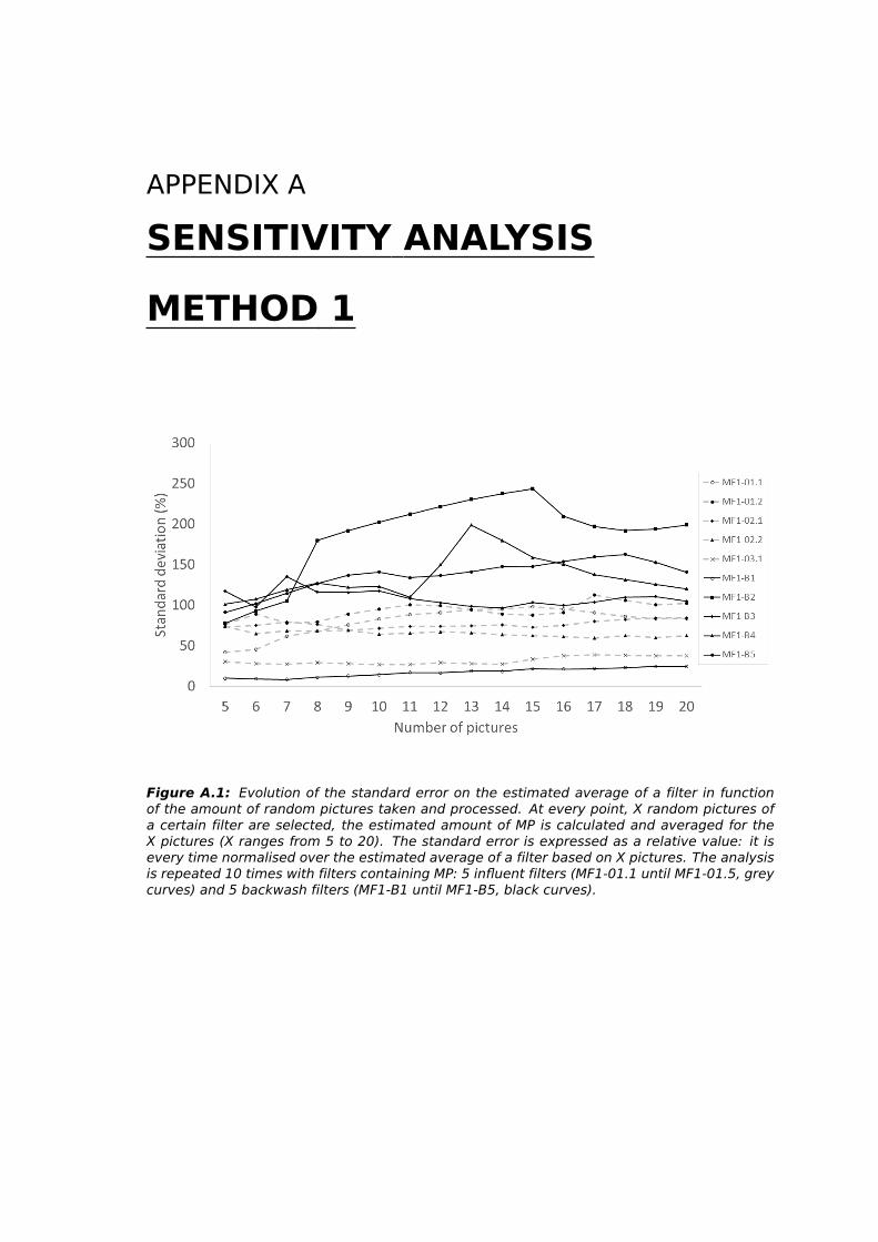
APPENDIX A
SENSITIVITY ANALYSIS
METHOD 1
Figure A.1: Evolution of the standard error on the estimated average of a filter in functionof the amount of random pictures taken and processed. At every point, X random pictures ofa certain filter are selected, the estimated amount of MP is calculated and averaged for theX pictures (X ranges from 5 to 20). The standard error is expressed as a relative value: it isevery time normalised over the estimated average of a filter based on X pictures. The analysisis repeated 10 times with filters containing MP: 5 influent filters (MF1-01.1 until MF1-01.5, greycurves) and 5 backwash filters (MF1-B1 until MF1-B5, black curves).
Recommended


