
Yan Kestens Æ Marius Theriault Æ Francois Des Rosiers
Heterogeneity in hedonic modelling of houseprices: looking at buyers’ household profiles
Received: 24 August 2004 / Accepted: 19 July 2005 / Published online: 15 November 2005� Springer-Verlag 2005
Abstract This paper introduces household-level data into hedonic models inorder to measure the heterogeneity of implicit prices regarding householdtype, age, educational attainment, income, and the previous tenure status ofthe buyers. Two methods are used for this purpose: a first series of modelsuses expansion terms, whereas a second series applies GeographicallyWeighted Regressions. Both methods yield conclusive results, showing thatthe marginal value given to certain property specifics and location attributesdo vary regarding the characteristics of the buyer’s household. Particularly,major findings concern the significant effect of income on the location rent aswell as the premium paid by highly-educated households in order to fulfilsocial homogeneity.
Keywords Hedonic modelling Æ Implicit prices Æ Heterogeneity Æ GWR ÆHousehold profile
JEL classification R20 Æ C50
Y. Kestens (&)Department of Social and Preventive Medicine, Universite de Montreal, 3875, St-Urbain,bureau 328, Montreal, Quebec H2W 1V1, CanadaE-mail: [email protected]: +1-514-4127142M. TheriaultCentre de Recherche en Amenagement et Developpement, Universite Laval, 1630-PavillonFelix-Antoine-Savard, Quebec, Quebec G1K 7P4, CanadaF. Des RosiersFaculty of Business Administration, Universite Laval, Quebec, Quebec G1K 7P4, Canada
J Geograph Syst (2006) 8: 61–96DOI 10.1007/s10109-005-0011-8
ORIGINAL ARTICLE

1 Introduction
The analysis of house prices using hedonic modelling makes it possible toestimate the marginal monetary contribution of property attributes andneighbourhood externalities (Rosen 1974). In most hedonic models, oneunique coefficient is derived for each observed attribute. It is entirely possiblethat this coefficient may vary according to some systematic pattern. Variousmethods have been designed to handle such variation (Anselin 1988;Brunsdon et al. 1996; Casetti 1972; Fotheringham et al. 2002; Griffith 1988).Explicitly integrating heterogeneity—which may be spatial—should improvethe calibration of the models while enhancing the understanding of theresidential market structure.
This paper presents an empirical case study analysing the spatial andsocial structure of residential property markets by combining single-familyproperty sales and household-level socio-economic data. Through the use oftwo context-sensitive hedonic methods—the Casetti expansion method(Casetti 1972, 1997) and geographically weighted regression (GWR)(Brunsdon et al. 1996; Fotheringham 2000; Fotheringham et al. 2002)—andtrough the incorporation of the socio-economic profile of actual propertybuyers, we have attempted to validate the following hypothesis: the vari-ability of the implicit prices of certain property and location attributes ispartly linked to individual preferences. In a recent dissertation, Kestens(2004) showed that the residential choice criteria—both as regards propertyand neighbourhood—vary significantly with the household profile, that is,with the type of household, age, income, educational attainment, the type ofprevious tenure (first-time owner vs. former owner), and even with the senseof belonging to the neighbourhood.
In order to investigate these questions, this paper analyses the variationof the impact of property-specifics and neighbourhood attributes consideringhousehold socio-economic profiles using hedonic modelling. Thereby, wehope to contribute to Starret’s (1981) debate on homogeneity of preferencesand capitalisation. As pointed out by Tyrvainen (1997), according to Starret,the capitalisation of an attribute is complete ‘‘if: (1) there is enough variationwithin the variable’—e.g. in order to measure the effect of proximity topower lines, it is important to account for cases where power lines are distantenough so as to prevent any effect on house prices—and ‘‘if (2) the residents’preferences are homogeneous. If the preferences are heterogeneous, capi-talisation is only partial’’ (Tyrvainen 1997, p. 220). Whereas the first con-dition can easily be controlled, the second has been the object of littleresearch. Thus, we hypothesize that the capitalisation is partial in that thevalue given to an attribute differs with household preferences. While such anassumption may seem to challenge the traditional interpretation of an he-donic function and to question the identification problem addressed byRosen (1974), it is supported by empirical evidence about the existence ofsub-markets and the heterogeneity of hedonic prices over space (Goodmanand Thibodeau 2003). We therefore feel that for adequately measuringthrough hedonic modelling the capitalisation of an attribute, residents’preferences for this attribute have to be homogeneous, or otherwise vary in a
62 Yan Kestens et al.

systematic way. In other words, part of the non-stationarity of the value ofproperty and location attributes may be linked to differences among thebuyer’s household profiles. Appropriate drift-sensitive regression techniquescan be used to validate this hypothesis when data is available at thehousehold level. One could argue that standard hedonic models implicitlyinclude buyer’s household profiles. Households of similar socio-economicprofile select properties in similar locales, the characteristics of which areaccounted for by the use of housing, neighbourhood and location variables.However, this paper explicitly tests the marginal effect of property buyerprofiles, beyond the average characteristics of the neighbourhood’s compo-sition.
The methods presented in this paper should not be considered a valuationtool but merely a way to better understand urban dynamics with respect tohouse price formation. Results are specific to Quebec City, Canada, and tothe socio-economic conditions prevailing in its property market for the 1993–2001 period. Vacancy rates were high and sellers abundant. In this context,advantages in the negotiation process are granted to the buyers, which canexplain some of our findings.
Two sets of hedonic models are built using some 761 single-propertyprices sold in Quebec City between 1993 and 2001. The first set uses Casetti-type interactive terms, while the second relies on GWR. Special attention isgiven to local indicators of spatial autocorrelation (LISA) (Anselin 1995), asit is expected that the introduction of disaggregated household-level datareduces the number of local spatial autocorrelation ‘‘hot spots’’. Section 2discusses the hedonic modelling technique, the spatial dimensions of prop-erty markets, and presents Casetti’s expansion method as well as the GWR.Section 3 presents the data bank and the modelling procedure, whereas theresults are given in Sect. 4. Finally, a summary of the main findings andfurther research possibilities are presented in Section 5.
2 Literature
2.1 Hedonic modelling
The hedonic framework relies on Lancaster’s consumer theory, stating thatutility is derived from the properties or characteristics of a good (Lancaster1966). Since this theory has been extended to the residential market by Rosen(1974), residential hedonic analysis has become widely used as an assessmenttool and for property market and urban analysis. The regression of houseprices on a variety of property specific and neighbourhood descriptorsevaluates their marginal contribution, also called implicit or hedonic prices.In their basic form, hedonic regressions assume each parameter to be fixed inspace, which means that each identified attribute has the same intrinsiccontribution throughout the submarket under study:
y ¼ Xbþ e ð1Þ
Heterogeneity in hedonic modelling of house prices 63
where y is a vector of selling prices, X a matrix of explanatory variables, b avector of regression coefficients, and � the error term.
However, property markets are very much tied as well as inherent in thespatial structure of the urban landscape. In fact, although capital is mobile,supply may be quite inelastic (Goodman and Thibodeau 1998), and aproperty, once constructed, becomes immovable, or spatially ‘‘rooted’’. As aresult, the value of a property is largely defined by its location attributes, thatis, by its relative location compared with urban infrastructure and services.Furthermore, as pointed out by Goodman and Thibodeau (1998), inelas-ticities in both supply and demand contribute to market segmentation. As arecent dissertation thesis has shown, the choice criteria concerning bothlocation and property choice vary depending on the household profile (Ke-stens 2004). This market segmentation may lead to heterogeneous implicitprices, which should be explicitly considered in the residential hedonic pricefunction. In fact, the implicit prices of the hedonic function reflect bothsupply- and demand-driven forces. In an equilibrium situation, it is assumedthat these forces cannot be distinguished within a hedonic function. How-ever, we believe that when the market conditions are not in equilibrium, butinstead those of a seller market (much supply for low demand), it becomespossible for the buyers to influence the price they pay for an amenity. If theconditions were reversed, that is, if it were a buyer market (much demand forlow supply), the sellers would have more power to impact upon the sellingprice, and the seller’s characteristics could then be significantly linked to thedrift of the implicit prices. Therefore, we assume that the introduction ofhousehold-level variables within the hedonic function using appropriatemethods like the Casetti expansions may make it possible to estimate thedrift in the coefficients associated with certain characteristics of the buyers.
2.2 Spatial dimensions of property markets
Can (1992) distinguishes two types of spatial effects: neighbourhood effectsand adjacency effects. The former refers to internalised values of geo-graphical features (exogenous effects), while the latter refers to spatial spill-over effects; that is, the impact of the characteristics of close surroundingproperties (endogenous effects). Exogenous effects can be manifold, rangingfrom city-wide structural factors (e.g. location rent) to local externalities (e.g.view on a high-voltage tower). These geographical features induce trendsinto housing expenditures that have to be explicitly incorporated into thehedonic function, if they are not removed before modelling.
Classical hedonic modelling would estimate fixed’ coefficients; however,above-mentioned market segmentation may lead to spatial heterogeneity,that is, to possible drifts’ in the estimated coefficients.
Independently from this contextual variation of the impact of housingattributes, similarity of prices between close properties may also be partlylinked to spatial spill-over (endogenous effect). Spatial spill-over occurswhen characteristics of surrounding or adjacent properties are internalised inthe property value, leading to spatial dependency or association. This spatialdependency cannot be modelled adequately using additional descriptive
64 Yan Kestens et al.
geographical variables, and necessitates the introduction of spatial autore-gressive (SAR) terms into the hedonic function:
y ¼ Xbþ qWyþ e ð2Þ
y ¼ Xbþ aWðy� XbÞ þ e ð3Þ
where X is the matrix of explanatory variables, � the error term, Wy aspatially lagged dependent variable, with W as the weight matrix,q anda thespatial autoregressive parameters, that is,q the degree to which the values atindividual locations depend on their neighbouring values, anda the degree towhich the values at individual locations depend on their neighbours’ resid-uals (Fotheringham et al. 2002 p. 23).
The SAR terms may take several forms. Most often, however, they areweighted lagged values of the dependent variable (Eq. 2) or of the error term(Eq. 3) (Anselin 1988; Griffith 1988; Kelejian 1995). Ordinary least squares(OLS) is not appropriate for SAR procedures that necessitate generalisedleast squares (GLS) or Maximum Likelihood (ML) estimations. However,OLS regression presents several advantages: it ‘‘has a well-developed theory,and has available a battery of diagnostic statistics that make interpretationseasy and straightforward’’ (Getis and Griffith 2002, p. 131). Spatiallydependent variables can also be transformed prior to modelling in theirspatial and non spatial components, using spatial filtering techniques (Cliffand Ord 1981; Getis 1995; Getis and Griffith 2002; Griffith 1996, 2000). Ofcourse, combinations of these methods can be used. For example, a modelintegrating geographical features accounting for the spatial drift may alsoinclude an autoregressive term controlling for spatial dependency. However,‘‘a two step procedure is considered to be more suitable’’ (Can 1990). Thatmeans that SAR terms should only be included if spatial dependency is stillpresent after spatial heterogeneity has been fully considered.
2.3 Methods and previous results
In this paper, the spatial heterogeneity of the parameters is handled usingtwo methods, namely, the spatial expansion method developed by Casetti(1972, 1997) and the Geographical Weighted Regression (Brunsdon et al.1996; Fotheringham et al. 2002). Furthermore, we observe how the intro-duction of detailed household-profile data helps explaining spatial hetero-geneity while diminishing spatial dependence.
The spatial expansion method developed by Casetti has first been used toanalyse the spatial drift inherent to various geographical phenomena likemigration (Casetti 1986), labor markets (Pandit and Casetti 1989) or priceanalyses before being applied to property market and price analysis (Atenand Heston 2005, Forthcoming; Can 1990, 1992; Casetti 1997). Theparameter drift refers to the variation of the parameter value depending onthe context. In fact, this method ‘‘extends’’ fixed parameters by introducinginteractive variables that combine a previously defined (fixed) characteristicwith a (spatially) dependent variable relating to the (spatial) context:
Heterogeneity in hedonic modelling of house prices 65

y ¼ ðCtðEþ IÞXÞbþ e ð4Þ
with C, a matrix of contextual variables which can be manifold (including avector of 1 values in the first column), E a matrix of expansion indicatingwhich explanatory variables are expanded by the contextual variables, andX, a matrix of explanatory variables, each one being activated in E.
In most models’ specifications, the estimation of varying parameters islimited to structural factors and the ‘‘contextual’’ variables mainly relate toneighbourhood characteristics [e.g. neighbourhood quality in Can (1990)].However, the expansion method can be applied more generally, by observingthe heterogeneity of any parameter X depending on the ‘‘context’’. This‘‘context’’ may refer to neighbourhood attributes (quality, distance to thecity centre, etc.), but also, as is suggested in this paper, to the specificcharacteristics of the buyers. The significant expansion parameters thereforemeasure the variation of the implicit prices people assign to attributes. Also,a parameter can be non significant overall, but may become significant oncecontextualised. This is only a special case of Eq. (4), that is, when b 0 is nulland b 1 is not.
Can (1990) measures the drift of several property specific parameters inrelation to the neighbourhood quality for a sample of 577 single-familyhouses of the Columbus metropolitan area. The two final models considerboth the spatial heterogeneity of property specifics (using spatial expansionto neighbourhood quality) and the spatial dependence (using a spatiallylagged dependent variable). The parameters that vary significantly throughspace are the following: the type of exterior, the lot size, the presence of atwo-car garage and the presence of a utility room. Recently, a model builtwith single-family properties transacted during the 1990–1991 period inQuebec City includes several expansion variables (Theriault et al. 2003).Various property attributes are spatially expanded using indicators of rela-tive centrality, family cycle and socio-economic status (derived from censusdata) as well as using measures of accessibility to regional and local services(computed within a GIS). In addition to age, lot size and connection to thesewer system, three property specifics present spatial drifts: inferior ceilingquality, kitchen cabinets made of hard wood, and the number of washrooms.It seems important to verify whether further drifts in the implicit prices couldbe related to the buyer’s household specific attributes acting on top of thespatial drifts related to social profiles of the neighbourhoods. This researchquestion follows recent findings that showed that the odds-ratio of men-tioning a property or neighbourhood choice criteria—i.e., a proxy of theirpreference for certain types of attributes—is significantly linked to thehousehold profile (Kestens 2004). To the best of our knowledge, no researchhas yet integrated household profile data into hedonic modelling.
Concomitantly with the expansion method, we ran several GWRs, whichgave additional indications on the spatial non-stationarity of the parameters.GWR is an adaptation of moving regressions. Moving regression functionsare calibrated for every point of a regular grid, using all data within a certainregion around this point. The resulting parameters are site-specific and cantherefore vary through space. However, this method is discontinuous, as noweighting schemes are applied to the data used for calibration.
66 Yan Kestens et al.

Geographically weighted regressions calibrate local models for everysampling point. However, a weighting scheme (spatial kernel) is applied inorder to give greater influence to close data points. Furthermore, the spatialkernel may be fixed (identical for all locations) or adaptive; that is, itsbandwidth may vary with the density of the data:
yi ¼ b0 ui; við Þ þX
kbk ui; við Þxik þ ei; ð5Þ
where (ui, vi) denotes the coordinates of the ith point in space and bk (ui, vi) isa realisation of the continuous function bk (u, v) at point i (Fotheringhamet al. 2002, p. 52).
Various methods can be used to derive the bandwidth that provides atrade-off between goodness-of fit and degrees of freedom: the generalisedcross-validation (GCV) criterion (Craven and Wahba 1979; Loader 1999),the Schwartz Information Criterion (Schwartz 1978) or the akaike infor-mation criterion (AIC) (Akaike 1973; Hurvich et al. 1998). For further de-tails on the spatial weighting function calibration, see Fotheringham et al.(2002, p. 59–62). Furthermore, the stationarity of each estimated parametercan be tested using either a Monte Carlo approach (Hope 1968) or the Leungtest (See Fotheringham et al. 2002, pp. 92–94; Leung et al. 2000).
In a GWR application on residential value analysis, Brunsdon et al.(1999) showed that the relationship between house price and size variessignificantly through space in the town of Deal in south-eastern England.
3 Modelling procedure
All models were built with 761 single-family properties transacted between1993 and 2001 in Quebec City, Canada (mainly between 1993 and 1996).Property-specific variables were extracted from the valuation role. Thecharacteristics of the vegetation around each property were extracted fromremote-sensing data. A Landsat TM-5 image shot in 1999 was categorisedusing the semi-automated ISODATA (iterative self-organising data analysis)technique, widely used and implemented in some GIS packages (Duda andHart 1973). Furthermore, the Normalised Difference Vegetation Index(NDVI), a sensitive indicator of the green biomass (Tucker 1979; Tueller1989; Wu et al. 1997), was derived. For more details about the extraction ofvegetation data from remote sensing images and its integration into hedonicmodels, see Kestens et al. (2004). NDVI is a measure of vegetation densitywhereas its standard deviation indicates land-use heterogeneity. An addi-tional variable identifies properties with more than 29 trees (according to thenumber of trees mentioned by the owners during a phone survey, as de-scribed below). Previous work by Payne identified this number as the limitupon which the premium accorded to trees was reversed (Payne 1973).Centrality—the mean car-time distance to the main activity centres(MACs)—was computed within a GIS (Theriault et al. 1999). Furthermore,a major phone survey carried out from 2000 to 2003 provided detailedinformation about each buyer household. The survey concerned the house-hold’s moving motivations and property choice criteria, and provided
Heterogeneity in hedonic modelling of house prices 67

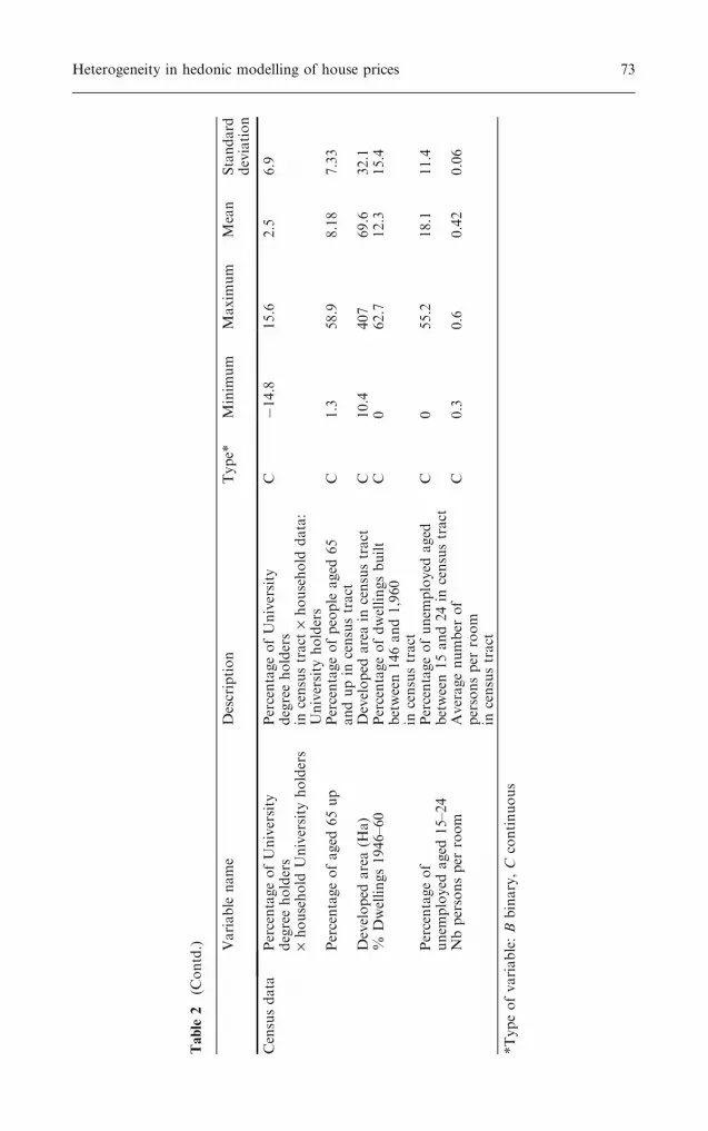
additional data on the household profiles and on specific attributes of theproperty, like the number of trees on the lot. A detailed description of thesurvey and the relations between the motivation to move, choice criteria andhousehold profile are given in Kestens (2004). A description of the variablesis presented in Tables 1 and 2.
3.1 Expansion models
In this paper, a first group of models, referred to as global models, is builtusing the expansion method. All models are in the semi-log functional form(the dependent variable is the logarithm of the selling price) using OLSspecification. The first four models (M) omit census variables, whereas thelast three (N) include them (see Table 3). A time-drift variable was intro-duced but did not prove significant. Concerning the M models, a basic model(M1) contains property specifics, vegetation attributes derived from remote-sensing data, and centrality measures, whereas homebuyers’ socio-economicvariables are added in a second step (M2). Expansion terms (all attributesbeing ‘‘expanded’’ with regard to the socio-economic profile of the buyers’households) are then added on to both model M1 (resulting in model M3)and model M2 (resulting in model M4). The N series is distinctive in that itcontains additional socio-economic Census variables, with N1 as the basicmodel (including property specifics, vegetation, centrality and Census data),N2 including household profile variables, while expansion terms are intro-duced in N3. In order to avoid multicollinearity, all expansion terms are builtwith the previously centered original variables, thereby reflecting thedeparture from the overall average market values (Jaccard et al. 1990, p. 31).
3.2 GWR models
Concomitantly, using the same dependent and explanatory variables as inM1, M2, N1 and N2, four Geographically Weighted Regressions are built(GWR_M1, GWR_M2, GWR_N1, and GWR_N2). The limitation of theGWR software available, confined to a maximum of 35 variables, made itimpossible to derive further GWR versions of models M3, M4 or N3.However, the interest of GWR relies in the possibility of deriving localstatistics and a significance test for the stationarity of individual parameters.For a description of further local descriptive statistics that can be obtainedusing the geographically weighting framework, see Brunsdon et al. (2002).An F-statistic also indicates the significance of improvement between theglobal and the GWR models. Furthermore, as M3, M4 and N3 are the‘‘expanded’’ versions of M1, M2 and N2, they can easily be compared withtheir GWR counterparts, GWR_M1, GWR_M2 and GWR_N2.
All the GWRs were computed with adaptive bi-square spatial kernels,using all data and the AIC minimisation for calibration of the spatialweighting function (Fotheringham et al. 2002, p. 61). The significance testfor the heterogeneity of the parameters was made using the Monte Carloapproach (Hope 1968).
68 Yan Kestens et al.

Table
1Descriptionofproperty
specificattributes
Variable
name
Description
Type*
Minim
um
Maxim
um
Mean
Standard
deviation
Property
specifics
SPRIC
ESale
price
oftheproperty
(Cad$)
C53,000
290,000
114,459
40,249
LNSPRIC
ENaturallogarithm
ofthesale
price
(Cad$)
C10.9
12.6
11.6
0.31
Localtaxrate
Localtaxrate
(/100ofassessedvalue)
C1.20
2.76
2.06
0.39
LivingareaM2
Livingarea(sqm)
C65.7
265.0
122.0
35.3
Age30–39
·livingarea
Livingarea(sqm)
·age30–39
�54.9
59.3
�1.8
16.4
Livingareabung.
Livingareaofabungalow
(sqm)
0206.6
49.7
52.2
Livingareabung
·income80K
up
Livingareaofabungalow
(sqm)
·Yearlyincome80,000Cad$up
�37.7
113.4
�3.6
24.2
LnLotsiz
Naturallogarithm
ofthelotsize
(sqm)
C5.3
7.5
6.3
0.3
App.age
Apparentage(years)
C0
54
16.6
12
App.age
·Single
Household
Apparentage(years)
·single
houshold
�15.6
22
0.1
2.7
Apparentagecentreedsquared
Apparentagecentreedsquared
C0.185
1401.0
143.8
160.1
Apparentagecentreedsquared
·household
income
Apparentagecentreedsquared
·household
income
C�3253.4
2662.2
30.4
501.1
Quality
House
quality
index
C�1
20.00
0.2
Finished
basement
Finished
basement
B0
10.56
0.50
Superiorfloorquality
Superiorfloorquality
B0
10.49
0.50
Facing51%+
brick
More
than50%
offacingmadeofstoneorbrick
B0
10.38
0.49
Built-in
oven
Built-in
oven
01
0.14
0.34
Built-in
oven
·age40–49
Built-in
oven
·age40–49
B�0.33
0.54
0.00
0.17
Fireplace
Numbersoffireplaces
C0
60.34
0.53
Fireplace
first-timeowner
Superiorfloorquality
C�2.72
0.86
�0.03
0.26
In-groundpool
Presence
ofanin-groundpool
B0
10.06
0.23
Heterogeneity in hedonic modelling of house prices 69

Table
1(C
ontd.)
Variable
name
Description
Type*
Minim
um
Maxim
um
Mean
Standard
deviation
In-groundpool
·household
income
Presence
ofanin-groundpool
·household
income
C�4.65
2.90
0.07
0.58
In-groundpool
·single
household
Presence
ofanin-groundpool
·single
household
C�0.13
0.82
�0.01
0.05
Detached
garage
Presence
ofadetached
garage
B0
10.12
0.33
Detached
garage
·University
degreeholders
Presence
ofadetached
garage
·University
degreeholder
C�0.48
0.40
0.00
0.16
Detached
garage
·couple
withoutchild
Presence
ofadetached
garage
·couple
withoutchildren
B�0.16
0.72
0.00
0.13
Detached
garage
·Age40–49
Presence
ofadetached
garage
·age40–49
B�0.33
0.55
�0.01
0.15
Att
garage
Presence
ofanattached
garage
B0
10.08
0.28
*Typeofvariable:B
binary,C
continuous
70 Yan Kestens et al.

Table
2Descriptionoflocationalandsocio-economic
attributes
Variable
name
Description
Type*
Minim
um
Maxim
um
Mean
Standard
deviation
Accessibility
Cartimeto
MACs
Cartimedistance
tomain
activitycenters
(min)
B4.685
21.0
12.6
3.51
CarTim
eto
MACsCdSqd
Cartimedistance
toMAC
centeredsquared(m
in)
B1E-06
70.9
12.3
14.7
Cartimeto
MACs
centeredsquared
·household
income
Cartimedistance
toMAC
centeredsquared(m
in)
·household
income
C�217.2
154.8
3.37
36.3
Highwayexit
Cartimedistance
tonearest
highwayexit(m
in.)
C0.04
7.53
2.74
1.46
Household-level
data
Household
income
Household
incomein
10,000$ranges
upto
100,000andup
C1
10
6.93
2.27
First-tim
eowners
Theowner
ofthisproperty
isowner
forthefirsttime
C0
10.48
0.50
Ageunder
30
Aged
under
30atdate
oftransaction
C0
10.04
0.20
Vegetation
Mature
trees100m
Percentageofareain
a100m
radius
covered
byresidentialuse
withmature
trees
C0
76
18.5
17.20
Mature
trees100m
·Age30–39
Percentageofareain
a100m
radius
covered
byresidentialuse
withmature
trees
·age30–39
�20.3
35.4
�1.19
8.11
Mature
trees500m
Percentageofareain
a500m
radius
covered
byresidentialuse
withmature
trees
C0.5
45.0
14.1
9.68
Low
tree
density
500m
Percentageofareain
a500m
radius
covered
byresidentialuse
withlow
tree
density
C2.6
34.3
16.8
5.97
Nbtrees29up
Number
oftreesontheproperty
is29andup
C0
10.03
0.18
Heterogeneity in hedonic modelling of house prices 71

Table
2(C
ontd.) Variable
name
Description
Type*
Minim
um
Maxim
um
Mean
Standard
deviation
Vegetation
Nbtrees
29up
·age40up
Number
oftrees
ontheproperty
is29andup
·age40andup
C�0.31
0.66
0.003
0.09
NDVIstandard
deviation1km
NDVIstandard
deviation
ina1km
radius
(landuse
heterogeneity
measure)
C0.18
0.60
0.32
0.06
Agriculturalland
100m
·University
degreeholders
Percentageofagriculturalland
withdispersedtreesin
a100m
radius
·University
degreeholders
C�21.5
6.68
�0.13
1.63
Agriculturalland100m
·age30–39
Percentageofagriculturallandwith
dispersedtreesin
a100m
radius
·age30–39
C�9.5
24.2
0.1209
1.7
Agriculturalland100m
·age40up
Percentageofagriculturallandwith
dispersedtreesin
a100m
radius
·age40andup
C�12.5
16.9
�0.1
1.4
Agriculturalland100m
·household
withchildren
Percentageofagriculturallandwith
dispersedtreesin
a100m
radius
·household
withchildren
C�11.0
10.0
0.0
1.3
Agriculturalland100m
·first-timeowner
Percentageofagriculturallandwith
dispersedtreesin
a100m
radius
·first-timeowner
C�11.9
20.4
0.07
1.6
NDVI40m
·age30–39
Norm
aliseddeviationvegetation
index
within
a40m
radius
(density
ofvegetation)
·age30–39
C�0.36
0.32
0.00
0.07
Woodlands500m
·single
household
Percentageofwoodlandsin
a500m
radius
·single
households
C�10.6
26.1
�0.3
3.5
Censusdata
Percentageof
University
degreeholders
Percentageofuniversity
degreeholdersin
censustract
C4.7
60.1
33.0
14.7
72 Yan Kestens et al.
Table
2(C
ontd.) Variable
name
Description
Type*
Minim
um
Maxim
um
Mean
Standard
deviation
Censusdata
PercentageofUniversity
degreeholders
·household
University
holders
PercentageofUniversity
degreeholders
incensustract
·household
data:
University
holders
C�14.8
15.6
2.5
6.9
Percentageofaged
65up
Percentageofpeople
aged
65
andupin
censustract
C1.3
58.9
8.18
7.33
Developed
area(H
a)
Developed
areain
censustract
C10.4
407
69.6
32.1
%Dwellings1946–60
Percentageofdwellingsbuilt
between146and1,960
incensustract
C0
62.7
12.3
15.4
Percentageof
unem
ployed
aged
15–24
Percentageofunem
ployed
aged
between15and24in
censustract
C0
55.2
18.1
11.4
Nbpersonsper
room
Averagenumber
of
personsper
room
incensustract
C0.3
0.6
0.42
0.06
*Typeofvariable:B
binary,C
continuous
Heterogeneity in hedonic modelling of house prices 73

For each model, global and local spatial autocorrelation of the residualsare measured, using Moran’s I for the former (Moran 1950) and Getis andOrd’s zG*I (Getis and Ord 1992; Ord and Getis 1995) for the latter.
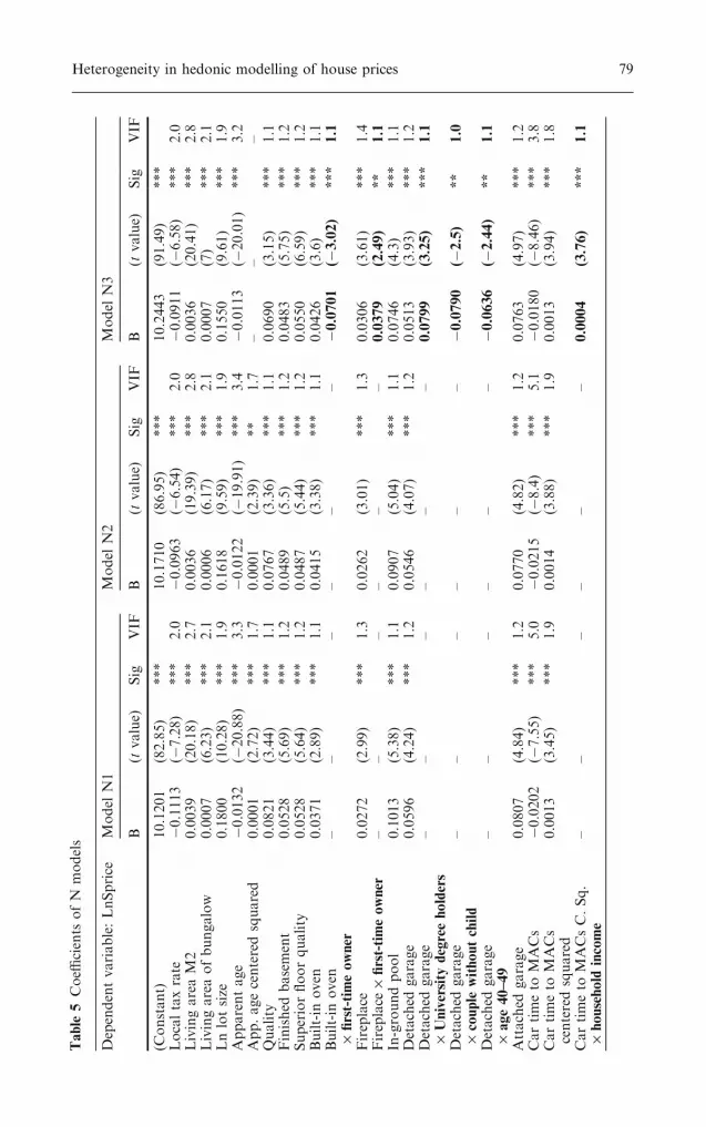
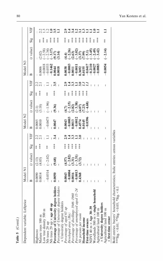
Table 3 contains the specifications and performance of all models. Theestimated parameters, their significance and the Variance Inflation Factor(VIF) values—indicating eventual multicollinearity—are detailed in Table 4(M series) and Table 5 (N series).
4 Results
4.1 Performance of the global models
Each of the global models explains at least 84% of the house price variation.The best model is N3, with an adjusted R-square of 0.889, a SEE of 10.9%,and an F value of 161. Collinearity is well under control in all models, withonly one VIF value slightly exceeding 5 (Car time to MACs, model N1).
No model presents any significant global spatial autocorrelation at the5% level (Moran’s I ranges from 0.034 [M4] to 0.172 [M1]). Local auto-correlation is present, but decreases when household-level data is included,and further more when expansion terms are introduced. The number of ‘‘hotspots’’, that we defined as the significant zG*i statistics given a 600 m lag(which is the most significant autocorrelation range according to the corre-logram), drops from 90 (M1) to 61 (M2) to 41 (M3) to 24 (M4). Results aresimilar for the N series that includes Census variables: the number of hotspots is already low for N1 (46), and still decreases for N2 (35) and N3 (26).The remaining local spatial autocorrelation in M4 and N3, as defined before,concerns less than 5% of the sample (respectively 24 and 26 cases out of 761,or 3.15% of all cases), and is as such not significant at the 95% confidencelevel.
The basic models M1 and N1 include classic descriptors as well as severalsignificant variables relating to vegetation, confirming the impact of envi-ronmental factors and surrounding land use on house values (Geogheganet al. 1997; Kestens et al. 2004).The percentage of trees has a global positiveimpact; however, when the socio-economic condition of the neighbourhoodis considered (Census data in Model N1), the impact of vegetation within a500 m range becomes non-significant. This stresses the links between thesocio-economic status of the neighbourhood and land use, mainly with re-gard to vegetation. Although mature trees in the close surroundings (100 maround the property) represent a premium, the presence of trees becomesdetrimental when exceeding a given threshold. In fact, the coefficient for thebinary variable identifying properties with more than 29 trees is significantlynegative (�5.90%, M1), in accordance with previous findings by Payne(1973).
Accessibility to the MACs is highly significant (t value of—11.02), but thenegative effect on property prices is not strictly linear, as proved by thepresence of the squared form of the parameter (previously centered to avoidcollinearity), with a positive sign (t value 4.41). Hence, the location rent
74 Yan Kestens et al.

Table
3Resultsofregressionmodels
Globalmodels
Withoutcensusdata
Withcensusdata
Model
M1
Model
M2
Model
M3
Model
M4
Model
N1
Model
N2
Model
N3
Model
specifications
Nbofcases
761
761
761
761
761
761
761
R-square
0.853
0.867
0.876
0.881
0.870
0.882
0.894
Adj.R-square
0.848
0.863
0.870
0.876
0.866
0.878
0.889
SEE
0.121
0.115
0.112
0.110
0.114
0.109
0.104
SEE(%
)12.9
12.2
11.9
11.6
12.1
11.5
10.9
Fratio
504
200
142
159
197
203
161
Sig.
0.0000
0.0000
0.0000
0.000
0.000
0.000
0.000
Df1/D
f223/737
24/736
36/723
34/727
25/735
27/733
38/722
Interactive
variables/totalvariables
0/23
0/24
13/36
12/34
0/25
0/27
11/38
Maxim
um
VIF
4.1
3.0
3.6
3.1
5.1
5.1
3.9
Spatial
auto-correlation
ofresiduals
Moran’sI(1,500m
lag)
0.172
0.130
0.084
0.034
0.176
0.159
0.102
Sig.
0.096
0.162
0.262
0.397
0.092
0.114
0.218
Most
sig.moran’sISA
range(300m
lags)
600m
600m
600m
600m
600m
600m
600m
Nbofsignificant
LISA
zG*i
statistics(600m
lag,sig.0.05)
90
61
41
24
46
35
26
Nbofsignificant
LISA
zGi
statistics(600m
lag,sig.0.05)
67
41
34
28
42
26
17
Variables
inmodel
Property
specifics
XX
XX
XX
XVegetationdata
XX
XX
XX
XCentrality
XX
XX
XX
XCensusdata
XX
XHousehold
variables
XX
XX
Heterogeneity in hedonic modelling of house prices 75

Table
3(C
ontd.)
Globalmodels
Withoutcensusdata
Withcensusdata
Model
M1
Model
M2
Model
M3
Model
M4
Model
N1
Model
N2
Model
N3
Variables
inmodel
Interactions(household
variables
·others)
XX
X
Geographicallyweightedregression(G
WR)models
Model
GWR_M1
Model
GWR_M2
Model
GWR_N1
Model
GWR_N2
GWR
models
Nbofcases
761
761
761
761
R-square
0.902
0.902
0.885
0.892
SEE
0.1061
0.1043
0.1098
0.1059
Number
ofneighbours
usedin
GWR
regressions
321
413
661
707
Fstatistic
ofGWR
improvem
ent(sig.)
3.36(0.002)
3.15(0.004)
2.78(0.008)
2.51(0.013)
Spatial
auto-correlation
ofresiduals
Moran’sI(1,500m
lag)
0.045
0.049
0.063
0.082
Sig.
0.364
0.352
0.316
0.265
NbofsignificantLISA
zG*istatistics(600m
lag,sig.0.05)
21
26
26
26
NbofsignificantLISA
zGistatistics(600m
lag,sig.0.05)
22
21
22
20
76 Yan Kestens et al.

Table
4Coeffi
cients
ofM
models
Dependentvariable:
LnSprice
Model
M1
Model
M2
Model
M3
Model
M4
B(t
value)
Sig
VIF
B(tvalue)
Sig
VIF
B(t
value)
Sig
VIF
B(t
value)
Sig
VIF
(Constant)
10.5479
(90.57)
***
10.6027
(97.15)
***
10.8351
(107.78)
***
10.7353
(108.71)
***
Localtaxrate
�0.1333
(�9.47)
***
1.5�0.1145
(�8.47)
***
1.5�0.1349
(�11.15)***
1.3�0.1211
(�10.15)***
1.3
LivingareaM2
0.0042
(20.6)
***
2.6
0.0039
(19.94)
***
2.7
0.0042
(22.35)
***
2.7
0.0039
(21.16)
***
2.7
Age30–39
·livingarea
––
––
––
0.0007
(2.98)
***
1.1
––
–Livingareabung.
0.0007
(6.15)
***
2.1
0.0007
(6.16)
***
2.1
0.0008
(7.52)
***
2.1
0.0008
(7.30)
***
2.1
Livingareabung.
·income80K
up
––
––
––
�0.0006
(�3.56)
***
1.1�0.0005
(�3.12)
***
1.1
LnLotsiz
0.1705
(9.17)
***
1.9
0.1511
(8.54)
***
1.9
0.1319
(7.59)
***
1.9
0.1346
(7.93)
***
1.9
App.age
�0.0132
(�20.01)***
3.2�0.0116
(�19.14)***
3.0�0.0123
(�19.99)***
3.2�0.0118
(�20.24)***
3.0
App.age
·single
household
––
––
––
0.0035
(2.24)
**
1.0
0.0044
(2.95)
***
1.0
App.agecenteredsquared
0.0001
(2.36)
**
1.7
0.0001
(1.81)
*1.7
0.0001
(2.00)
**
1.8
0.0000
(2.26)
**
1.8
App.agecenteredsquared
·household
income
––
––
––
0.0001
(5.39)
***
1.3
––
–
Quality
0.0933
(3.67)
***
1.1
0.0883
(3.65)
***
1.1
0.0780
(3.27)
***
1.1
0.0624
(2.68)
***
1.1
Finished
basement
0.0509
(5.16)
***
1.2
0.0485
(5.15)
***
1.2
0.0577
(6.24)
***
1.2
0.0526
(5.82)
***
1.2
Superiorfloorquality
0.0566
(5.7)
***
1.2
0.0508
(5.35)
***
1.2
0.0605
(6.54)
***
1.2
0.0529
(5.85)
***
1.2
Facing51%+
brick
0.0268
(2.76)
***
1.1
0.0193
(2.08)
**
1.1
0.0272
(�3.00)
***
1.1
0.0216
(2.44)
**
1.1
Built-in
oven
0.0414
(3.04)
***
1.1
0.0437
(3.39)
***
1.1
0.0465
(3.66)
***
1.1
0.0534
(4.33)
***
1.1
Built-in
oven
·age40–49
––
––
––
0.0581
(2.3)
**
1.0
0.0657
(2.68)
***
1.0
Fireplace
0.0259
(2.67)
***
1.3
0.0237
(2.57)
***
1.3
0.0368
(3.98)
***
1.4
0.0341
(3.79)
***
1.4
Fireplace
·first-timeowner
––
––
––
0.0465
(2.81)
***
1.1
0.0448
(2.80)
***
1.1
In-groundpool
0.1068
(5.33)
***
1.1
0.0940
(4.93)
***
1.1
0.0750
(3.51)
***
1.4
0.0645
(3.14)
***
1.4
In-groundpool
·household
income
––
––
––
0.0358
(3.93)
***
1.7
0.0205
(2.61)
***
1.3
In-groundpool
·single
household
––
––
––
0.2985
(3.20)
***
1.5
––
–
Detached
garage
0.0510
(3.42)
***
1.2
0.0440
(3.1)
***
1.2
0.0508
(3.63)
***
1.2
0.0427
(3.12)
***
1.2
Detached
garage
·University
degreeholders–
––
––
–0.0714
(2.72)
***
1.0
0.0864
(3.37)
***
1.0
Detached
garage
·couple
withoutchild
––
––
––
�0.0810
(�2.37)
**
1.0�0.0812
(�2.42)
**
1.0
Heterogeneity in hedonic modelling of house prices 77

Table
4(C
ontd.)
Dependentvariable:
LnSprice
Model
M1
Model
M2
Model
M3
Model
M4
B(t
value)
Sig
VIF
B(t
value)
Sig
VIF
B(t
value)
Sig
VIF
B(t
value)
Sig
VIF
Detached
garage
·age40–49
––
––
––
�0.0559
(�1.99)
**
1.0�0.0800
(�2.92)
***
1.0
Attached
garage
0.0770
(4.34)
***
1.2
0.0687
(4.08)
***
1.2
0.0682
(4.09)
***
1.2
0.0592
(3.64)
***
1.2
Cartimeto
MACs
�0.0250
(�11.02)***
3.2�0.0271
(�13.1)
***
2.9�0.0223
(�12.49)***
2.3�0.0233
(�13.44)***
2.3
Cartimeto
MACs
centeredsquared
0.0017
(4.41)
***
1.6
0.0018
(5.06)
***
1.6
0.0011
(3.24)
***
1.6
0.0015
(4.51)
***
1.6
Cartimeto
MACscentered
squared
·household
income
––
––
––
0.0004
(3.12)
***
1.2
0.0005
(4.23)
***
1.1
Mature
trees100m
0.0010
(2.42)
**
2.9
––
––
––
Mature
trees100m
·age30–39
––
––
––
0.0007
(1.79)
*3.0
––
–
Mature
trees500m
0.0041
(4.44)
***
4.0
0.0036
(5.41)
***
2.4
0.0037
(4.59)
***
3.6
0.0039
(6.22)
***
2.3
Low
tree
density
500m
�0.0034
(�3.32)
***
2.0�0.0026
(�2.9)
***
1.6�0.0033
(�3.88)
***
1.6�0.0037
(�4.49)
***
1.5
Nbtrees29up
�0.0609
(�2.25)
**
1.1�0.0629
(�2.45)
**
1.1�0.0689
(�2.71)
***
1.1�0.0617
(�2.47)
**
1.1
Nbtrees29up
·age40up
––
––
––
––
––
�0.1653
(�3.37)
***
1.0
NDVIstandard
deviation1km
0.2893
(2.87)
***
2.1
0.2217
(2.46)
**
1.8
––
––
––
–
Household
income
––
–0.0166
(7.91)
***
1.3
––
––
0.0172
(8.47)
***
1.3
First-tim
eowners
––
–�0.0427
(�4.72)
***
1.1
––
––
�0.0402
(�4.69)
***
1.1
Ageunder
30
––
–�0.0390
(�1.75)
*1.0
––
––
––
–Agriculturalland100m
·University
degreeholders
––
––
–�0.0093
(�3.54)
***
1.1
––
–
Agriculturalland100m
·age30–39
––
––
–�0.0091
(�3.50)
***
1.1
––
–
Agriculturalland100m
·age40up
––
––
––
––
0.0098
(3.21)
***
1.1
Agriculturalland100m
·household
withchildren
––
––
––
––
0.0099
(3.09)
***
1.0
Bold
entries:buyers’household
characteristics;Italicentries:censusvariables
***Sig.<
0.01;**Sig.<
0.05;*Sig.<
0.1
78 Yan Kestens et al.
Table
5Coeffi
cients
ofN
models
Dependentvariable:LnSprice
Model
N1
Model
N2
Model
N3
B(t
value)
Sig
VIF
B(tvalue)
Sig
VIF
B(t
value)
Sig
VIF
(Constant)
10.1201
(82.85)
***
10.1710
(86.95)
***
10.2443
(91.49)
***
Localtaxrate
�0.1113
(�7.28)
***
2.0
�0.0963
(�6.54)
***
2.0
�0.0911
(�6.58)
***
2.0
LivingareaM2
0.0039
(20.18)
***
2.7
0.0036
(19.39)
***
2.8
0.0036
(20.41)
***
2.8
Livingareaofbungalow
0.0007
(6.23)
***
2.1
0.0006
(6.17)
***
2.1
0.0007
(7)
***
2.1
Lnlotsize
0.1800
(10.28)
***
1.9
0.1618
(9.59)
***
1.9
0.1550
(9.61)
***
1.9
Apparentage
�0.0132
(�20.88)
***
3.3
�0.0122
(�19.91)
***
3.4
�0.0113
(�20.01)
***
3.2
App.agecenteredsquared
0.0001
(2.72)
***
1.7
0.0001
(2.39)
**
1.7
––
–Quality
0.0821
(3.44)
***
1.1
0.0767
(3.36)
***
1.1
0.0690
(3.15)
***
1.1
Finished
basement
0.0528
(5.69)
***
1.2
0.0489
(5.5)
***
1.2
0.0483
(5.75)
***
1.2
Superiorfloorquality
0.0528
(5.64)
***
1.2
0.0487
(5.44)
***
1.2
0.0550
(6.59)
***
1.2
Built-in
oven
0.0371
(2.89)
***
1.1
0.0415
(3.38)
***
1.1
0.0426
(3.6)
***
1.1
Built-in
oven
·first-timeowner
––
––
––
�0.0701
(�3.02)
***
1.1
Fireplace
0.0272
(2.99)
***
1.3
0.0262
(3.01)
***
1.3
0.0306
(3.61)
***
1.4
Fireplace
·first-timeowner
––
––
––
0.0379
(2.49)
**
1.1
In-groundpool
0.1013
(5.38)
***
1.1
0.0907
(5.04)
***
1.1
0.0746
(4.3)
***
1.1
Detached
garage
0.0596
(4.24)
***
1.2
0.0546
(4.07)
***
1.2
0.0513
(3.93)
***
1.2
Detached
garage
·University
degreeholders
––
––
––
0.0799
(3.25)
***
1.1
Detached
garage
·couple
withoutchild
––
––
––
�0.0790
(�2.5)
**
1.0
Detached
garage
·age40–49
––
––
––
�0.0636
(�2.44)
**
1.1
Attached
garage
0.0807
(4.84)
***
1.2
0.0770
(4.82)
***
1.2
0.0763
(4.97)
***
1.2
Cartimeto
MACs
�0.0202
(�7.55)
***
5.0
�0.0215
(�8.4)
***
5.1
�0.0180
(�8.46)
***
3.8
Cartimeto
MACs
centeredsquared
0.0013
(3.45)
***
1.9
0.0014
(3.88)
***
1.9
0.0013
(3.94)
***
1.8
Cartimeto
MACsC.Sq.
·household
income
––
––
––
0.0004
(3.76)
***
1.1
Heterogeneity in hedonic modelling of house prices 79
Table
5(C
ontd.)
Dependentvariable:LnSprice
Model
N1
Model
N2
Model
N3
B(t
value)
Sig
VIF
B(t
value)
Sig
VIF
B(t
value)
Sig
VIF
Highwext
0.0090
(2.13)
**
2.2
0.0085
(2.1)
**
2.2
––
–Mature
trees100m
0.0014
(4.05)
***
2.1
0.0010
(3.18)
***
2.1
0.0006
(2.02)
**
2.2
Low
tree
density
500m
––
––
––
�0.0018
(�2.58)
***
1.3
Nbtrees29up
�0.0514
(�2.02)
**
1.1
�0.0475
(�1.96)
**
1.1
�0.0553
(�2.34)
**
1.2
Nbtrees29up
·age40up
––
––
––
�0.1462
(�3.17)
***
1.0
PercentageofUniversity
degreeholders
0.0050
(9.68)
***
3.4
0.0047
(9.36)
***
3.5
0.0044
(9.17)
***
3.5
PercentageofUniversity
degreeholders
·University
degreeholders
––
––
––
0.0018
(3.14)
***
1.1
Percentageofaged
65up
0.0043
(4.57)
***
2.9
0.0043
(4.7)
***
2.9
0.0038
(4.4)
***
2.9
Developed
area(Ha)
�0.0004
(�2.82)
***
1.4
�0.0003
(�2.15)
**
1.4
�0.0003
(�2.26)
**
1.4
Percentageofdwellings1946–1960
0.0016
(3.31)
***
3.3
0.0013
(2.82)
***
3.3
0.0011
(2.63)
***
3.4
Percentageofunem
ployed
aged
15–24
�0.0013
(�3.31)
***
1.1
�0.0012
(�3.38)
***
1.1
�0.0011
(�3.02)
***
1.2
Nbpersonsper
room
0.4368
(3.72)
***
3.0
0.4574
(4.07)
***
3.0
0.3692
(3.37)
***
3.1
Household
income
––
–0.0145
(7.23)
***
1.3
0.0155
(7.99)
***
1.3
First-tim
eowners
––
–�0.0396
(�4.68)
***
1.1
�0.0417
(�5.1)
***
1.1
NDVI40m
·Age30–39
––
––
––
�0.2110
(�3.45)
***
1.1
Woodlands500m
·single
household
––
––
––
�0.0027
(�2.49)
**
1.0
Agriculturalland100m
·University
degreeholders
––
––
––
�0.0083
(�3.42)
***
1.1
Agriculturalland100m
·first-timeowner
––
––
––
�0.0054
(�2.14)
**
1.1
Bold
entries:buyers’household
characteristics;Italicentries:censusvariables
***Sig.<
0.01;**Sig.<
0.05;*Sig.<
0.1
80 Yan Kestens et al.

follows a quadratic function and takes the form of a U-shaped curve, withpositive premiums both in the city centre and in the outer suburbs, ceterisparibus. A previous study showed that land-use and vegetation attributessignificantly explain part of these premiums, reducing the value and signifi-cance of the squared distance term (Kestens et al. 2004). Therefore, if veg-etation descriptors were absent, this parameter would be even higher andmore significant.
4.2 Introduction of socio-economic variables describing the household
Three variables describing the household are significant : the household in-come and the previous tenure status (Models M2, M4, N2 and N3) as well asthe age of the respondent at transaction date (under 30) (Model M2 only).Ceteris paribus,
– For each additional $10,000 of income, buyers pay an average premium of1.61% (1.46–1.73%, depending on the model)
– First-time owners pay between 4.04 to 4.36% less than former owners– Young households, under 30 years of age, pay 3.98% less than olderbuyers for the same property (only model M2, and sig 0.1).
Whether Census variables—describing the socio-economic profile of theneighbourhood at the Census-tract level—are included or not in the model,the two household-level variables Household Income and First-time Ownersstay significant, with similar and high t values (ranging from 7.23 to 8.47 andfrom 4.68 to 5.1, respectively, depending on the model). Furthermore, nosignificant collinearity is detected between the two levels of socio-economicmeasures (Census data and household data), the maximum VIF value amongthese variables being 3.5 (Percentage of university degree holders in theCensus tract, model N2).
Concerning the dichotomous age variable (Under 30), it is present in onemodel only (M2), with a low significance test (t value �1.75, sig. 0.1). Al-though it does not present any collinearity with household income or pre-vious tenure status as could have been expected, this variable drops out whenCensus data (N2) or further expansion terms are included (M3, M4, N3).
4.3 Adding expansion terms: controlling for heterogeneity
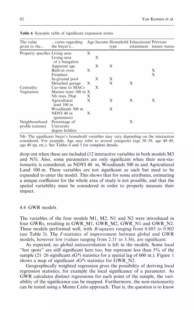
In a last step, we introduced expansion terms allowing for the basicparameters [property specifics, accessibility, vegetation (M3 and M4) andCensus data (N3)] to vary with regard to the household profile. Severalexpansion terms are significant, showing that the value given to certainproperty specifics or location attributes is not homogeneous among buyers.Table 6 presents the list of the parameters that are heterogeneous consid-ering the household characteristics of the buyers.
While a majority of expansion terms (15) is significant when both Censusdata and raw household profile variables are omitted (Model M3), only a few
Heterogeneity in hedonic modelling of house prices 81
drop out when these are included (12 interactive variables in both models M3and N3). Also, some parameters are only significant when their non-sta-tionarity is considered, as NDVI 40 m, Woodlands 500 m and AgriculturalLand 100 m. These variables are not significant as such but need to beexpanded to enter the model. This shows that for some attributes, estimatinga unique coefficient for the whole area of study is not possible, and that thespatial variability must be considered in order to properly measure theirimpact.
4.4 GWR models
The variables of the four models M1, M2, N1 and N2 were introduced infour GWRs, resulting in GWR_M1, GWR_M2, GWR_N1 and GWR_N2.These models performed well, with R-squares ranging from 0.885 to 0.902(see Table 3). The F-statistics of improvement between global and GWRmodels, however low (values ranging from 2.51 to 3.36), are significant.
As expected, no global autocorrelation is left in the models. Some local‘‘hot spots’’ are still significant here too, but represent less than 5% of thesample (21–26 significant zG*i statistics for a spatial lag of 600 m.). Figure 1shows a map of significant zG*i statistics for GWR_N2.
Geographically weighted regression gives the possibility of deriving localregression statistics, for example the local significance of a parameter. AsGWR calculates distinct regressions for each point of the sample, the vari-ability of the significance can be mapped. Furthermore, the non-stationaritycan be tested using a Monte Carlo approach. That is, the question is to know
Table 6 Synoptic table of significant expansion terms
The valuegiven to the...
...varies regardingthe buyer’s...
Age Income Householdtype
Educationalattainment
Previoustenure status
Property specifics Living area XLiving areaof a bungalow
X
Apparent age X XBuilt-in oven X XFireplace XIn-ground pool X XDetached garage X X X
Centrality Car-time to MACs XVegetation Mature trees 100 m X
Nb trees 29up XAgriculturalland 100 m
X X X X
Woodlands 500 m XNDVI 40 m(greenness)
X
Neighbourhoodprofile (census)
Percentage ofUniversitydegree holders
X
Nb: The significant buyer’s household variables may vary depending on the interactionconsidered. For example, Age may refer to several categories (age 30–39, age 40–49,age 40 up, etc.). See Tables 4 and 5 for complete details.
82 Yan Kestens et al.
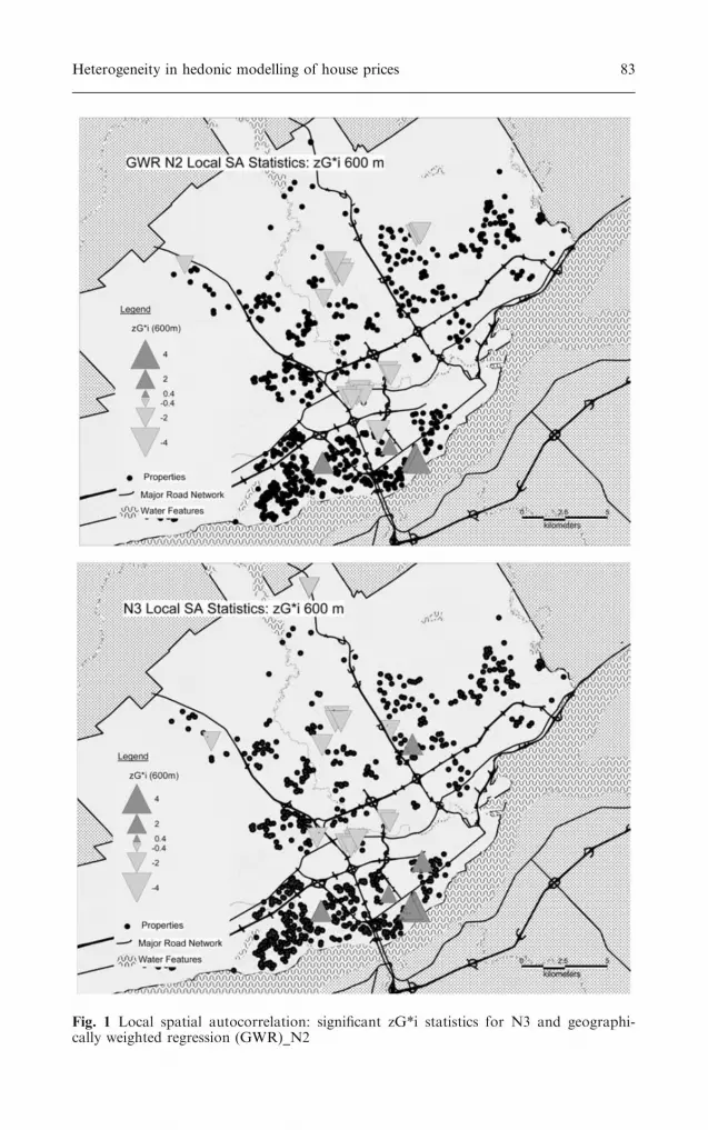
Fig. 1 Local spatial autocorrelation: significant zG*i statistics for N3 and geographi-cally weighted regression (GWR)_N2
Heterogeneity in hedonic modelling of house prices 83

whether the observed variation is sufficient to say that the parameter is notglobally fixed. p values testing for non-stationarity are given in Table 7. Forthe parameters with non-significant p values, it is assumed that a uniquecoefficient holds true. The parameters that are considered non-stationary aretherefore the following: local tax rate, apparent age (Fig. 2), Car Time toMACs (Fig. 3), NDVI Stdd. 1 km (GWR_M1 and GWR_M2), and %University Degree Holders (GWR_N1). Also, local R-squares give furtherindication about the fit of the model depending on location. However, thevalue of the local R-square is also influenced by the stationarity of the
Table 7 Non-stationarity of parameters in GWR Models (p values) and Moran’s Istatistic
Parameter p value Moran’s I(1,500 m)
GWR-M1 GWR-M2 GWR-N1 GWR-N2
(Constant) 0.02 0.06 0.39 0.32Local tax rate 0.00 0.00 0.08 0.10 0.66Living area m2 0.10 0.17 0.58 0.53 0.47Living area bung. 0.27 0.39 0.56 0.79 0.53Ln lot size 0.07 0.10 0.16 0.11 0.94App. age 0.01 0.02 0.27 0.40 1.10App. age centered squared 0.50 0.49 0.60 0.77 0.98Quality 0.24 0.32 0.49 0.38 0.04Finished basement 0.26 0.17 0.35 0.34 0.08Superior floor quality 0.32 0.30 0.25 0.38 0.31Facing 51%+ brick 0.50 0.24 – – 0.44Built-in oven 0.15 0.04 0.38 0.37 0.08Fireplace 0.64 0.76 0.36 0.20 0.29In-ground pool 0.88 0.90 0.45 0.62 0.07Detached garage 0.38 0.48 0.32 0.59 0.29Attached garage 0.90 0.67 0.71 0.40 0.02Car time to MACs 0.00 0.02 0.17 0.32 0.78Car time to MACscentered squared
0.00 0.00 0.13 0.21 0.96
Highway exit – – 0.09 0.22 0.81Mature trees 100 m 0.75 – 0.37 0.28 0.88Mature trees 500 m 0.49 0.32 – – 1.09Low tree density 500 m 0.15 0.08 – – 0.60Nb trees 29 up 0.58 0.58 0.41 0.28 0.02NDVI Standarddeviation 1 km
0.00 0.00 – – 0.95
Household income – 0.45 – 0.41 0.27First-time owners – 0.73 – 0.97 �0.11Age under 30 – 0.41 – – �0.05Percentage ofUniversity degree holders
– – 0.01 0.13 0.80
Percentage of aged 65 up – – 0.89 0.46 0.75Developped area (Ha) – – 0.11 0.17 0.81Percentage ofdwellings 1946–1960
– – 0.87 0.90 0.90
Percentage ofunemployed aged 15–24
– – 0.22 0.28 1.30
Nb persons per room – – 0.66 0.60 0.59
Italic entries: census data variables; Bold: buyers’ household variablesBold numbers: significant at the 95% confidence level
84 Yan Kestens et al.
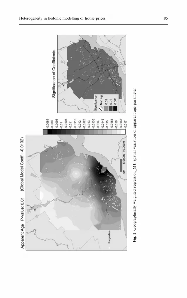
Fig.2
Geographicallyweightedregression_M1:spatialvariationofapparentageparameter
Heterogeneity in hedonic modelling of house prices 85

Fig.3
Geographicallyweightedregression_M1:spatialvariationofcar-timeto
MACscoeffi
cients
NB:the
non-significance
ofthecoeffi
cients
incertain
areasis
partly
dueto
thescarcepresence
ofsingle-family
properties,asforexample
inthemore
centralpositive-signarea
86 Yan Kestens et al.
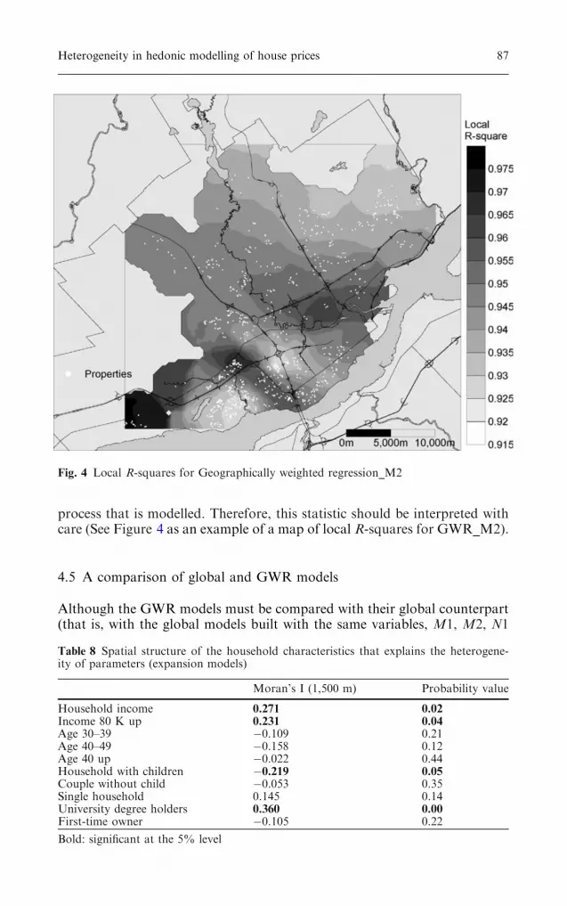
process that is modelled. Therefore, this statistic should be interpreted withcare (See Figure 4 as an example of a map of local R-squares for GWR_M2).
4.5 A comparison of global and GWR models
Although the GWR models must be compared with their global counterpart(that is, with the global models built with the same variables, M1, M2, N1
Fig. 4 Local R-squares for Geographically weighted regression_M2
Table 8 Spatial structure of the household characteristics that explains the heterogene-ity of parameters (expansion models)
Moran’s I (1,500 m) Probability value
Household income 0.271 0.02Income 80 K up 0.231 0.04Age 30–39 �0.109 0.21Age 40–49 �0.158 0.12Age 40 up �0.022 0.44Household with children �0.219 0.05Couple without child �0.053 0.35Single household 0.145 0.14University degree holders 0.360 0.00First-time owner �0.105 0.22
Bold: significant at the 5% level
Heterogeneity in hedonic modelling of house prices 87
and N2), it is also of interest to compare the GWRs with the expandedversions of the global specifications. For example, let us compare the two‘‘drift’’-sensitive versions of N2, that is N3 and GWR_N2. In both cases, thepercentage of explanation of the variance is similar (0.894 for the globalversion, vs. 0.892 for the GWR), as is the global autocorrelation of theresiduals (Moran’s I values respectively 0.102 and 0.0802). Concerning thelocal autocorrelation, the number of significant zG*i statistics (26) is iden-tical, although these hot spots do not strictly match spatially (See Fig. 1). Inthe end, these models are similar in terms of explanation power and for theirability to handle spatial autocorrelation.
Let us compare more precisely how these models handle heterogeneity.For N3, the coefficients that vary spatially are identified by the significantexpansion terms. These expansions refer to the following variables: built-inoven, fireplace, detached garage, car time to MACs, Nb of trees 29 up,percentage of University degree holders, NDVI 40 m (greenness) Woodlands500 m and agricultural land 100 m. The statistical significance of expansionterms indicates that for these variables, a single coefficient is not a validalternative. In fact, we know that the impact of these variables variesaccording to age, income, educational attainment and type of household.However, no local measure of significance is available.
For the GWRs, the heterogeneity of the parameters is given by the pvalues measured through a Monte Carlo procedure (Table 7). According tothese p values, four parameters vary significantly at the 95% confidence levelfor GWR_M1 and GWR_M2 [local tax rate, apparent age, car time toMACs (linear and squared form) and NDVI Stdd. 1 km (heterogeneity ofland use), one for GWR_N1 (percentage of university degree holders), andnone for GWR_N2. It is interesting to note that each of these variablesidentified as non-stationary is also strongly spatially structured, as indicatethe corresponding high Moran’s I statistics (Table 7, fourth column). Also,the findings suggest that for the variables with non-significant p values, aunique coefficient is adapted, that is, the implicit price is homogeneousamong the observations. This is a priori in contradiction with the findings ofthe global models using expansion terms. One could argue that the hetero-geneity identified in the expansion models refers to the household hetero-geneity, and not specifically to spatial heterogeneity, as it would have beenhad the attributes been expanded according to their coordinates (through theuse of trend surface analysis for example).
In fact, some of the variables describing the household profile are notspatially structured, as indicate the Moran’s I values shown in Table 8. Forthe attributes that have been expanded with these ‘‘non-spatial’’ householdcharacteristics, it is to be expected that they are not identified in the GWRframework as spatially heterogeneous (although other dimensions thanhousehold profile and preferences could be the cause of heterogeneity).However, both the income (Household Income and Income 80 K up) and theeducational attainment of the households (University degree holders) dopresent a spatial structure, with significant Moran’s I values at the 95%confidence level. The attributes that are significantly expanded in the globalmodels with these two characteristics should also be identified in the GWRmodels as heterogeneous, that is, with significant p values. This concerns the
88 Yan Kestens et al.
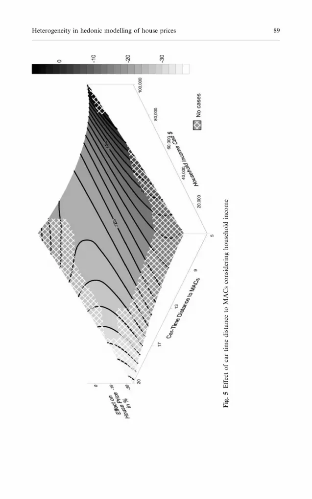
Fig.5
Effectofcartimedistance
toMACsconsideringhousehold
income
Heterogeneity in hedonic modelling of house prices 89
following: living area of a bungalow, in-ground pool, detached garage, cartime to MACs and percentage of University degree holders. Whereas the twolatter values are identified in the GWR as heterogeneous, the three formerones are not.
Concomitantly, two variables are considered heterogeneous within theGWRs, but are not significantly expanded in the global models (local taxrate) and NDVI Stdd. 1 km [land-use heterogeneity]). We can assume thatthe heterogeneity associated with these two attributes is not related tovariations in the household profiles.
Both methods yield highly interesting results. Whereas spatial expansionmakes it possible to consider both the spatial and the non-spatial hetero-geneity of parameters, GWR provides interesting information through localregression statistics. However, although GWR is an interesting tool toidentify and spatially describe non-stationary processes, it does not identifythe cause of the parameter drift. Spatial expansion on the contrary, althoughless precise locally, makes it possible to investigate the cause of non-sta-tionarity, thereby helping to disentangle the complex interactions influencingproperty values.
4.6 Some provocative findings
4.6.1 Accessibility and income
It is worthwhile to underline the significant drift of accessibility (car time toMACs, under its squared form) regarding household income. The car time toMACs is negatively linked to property values: each additional minute awayfrom the city centre lowers the property value of 1.82%. However, thisrelation is not strictly linear but rather follows a U-shaped curve form, asshown by the significant integration of the squared form of the variable, witha positive sign. Furthermore, this squared term significantly interacts withthe household income, with a positive sign too. This shows that the higherthe income, the higher the squared term. Therefore, the devaluation asso-ciated with distance is more important for low-income than for high-incomehouseholds, as shown on the three-dimensional surface of Fig. 5. This tendsto corroborate the distance-cost trade-off theory, stating that high-incomehouseholds can afford additional transportation costs and are ready to paymore for properties located in the outer-city limits. Also, the increasingpractice of telework, which particularly concerns managers and profession-als, may have an effect on the propensity of the most highly educated peopleto locate in more remote areas of the urban scene. In fact, those who canspend some working days at home may be willing to pay more for non-central locations, thus benefiting more from premium environments thantypical commuters. These findings lead to further investigation using 2001Origin-destination survey for Quebec City to analyze the spatial distributionof higher income telecommuters.
90 Yan Kestens et al.

4.6.2 Social homogeneity
As foreseen, the percentage of university degree holders in the census tracthas a global positive effect on the property value, each additional 10%adding a premium of 4.41%. This variable is among the most significantones, with a t value of 9.17. Additionally, the expansion with the household-level binary variable ‘‘Holding a university degree’’ marginally proved sig-nificant, with an additional 1.81% premium. This shows that all things beingequal, highly educated buyers who select single-family housing are willing topay more in their quest for social homogeneity.
4.7 Summary and conclusions
This paper aims at understanding how the marginal value given to propertyand location attributes may vary among buyers. A telephone survey wasconducted in order to obtain detailed information about 761 households thatacquired single-family properties in Quebec, Canada, during the 1993–2001period. Household-level attributes were introduced into hedonic functions tomeasure the effect of the homebuyer’s socio-economic context on implicitprices. Both the expansion method (Casetti 1972, 1997) and GWR (Foth-eringham et al. 2002; Fotheringham et al. 1998) are used to assess theeventual heterogeneity of the impact of property specifics and locationattributes.
A major finding is that some characteristics of the buyer’s household havea direct impact on property prices, namely the household income, the pre-vious tenure status, and age. These findings must be put into the perspectiveof a specific location (Quebec City) and specific market conditions, that is,mainly a seller market with high supply and rather low demand for housing,at least for most of the period considered. Under these particular conditions,and using appropriate space-sensitive interaction methods, we could showthat for each additional $10,000 of income, a buyer pays a premium of1.61% on average (+1.46 to 1.73%), all other things being equal. Also, themarginal effect of the household income is the fifth most significantparameter after the size (living area), the age of the property (apparent age),the social status of the neighbourhood (percentage of university degreeholders in the Census tract), and accessibility (Car Time to MACs) (N3).Several hypotheses can explain the parameter significance and its positivesign. First, it is possible that the lack of descriptors defining the luxuryattributes of the higher segment of the property market may result in apremium appearing as associated to the buyer’s income. However, as theirability to pay is increased, high-income buyers may also be less willing toengage in lengthy price negotiations, and may accept higher selling prices.Concomitantly, households with more restricted financial means may takemore time to find the ‘‘best’’ deal as their budget is inflexible. While takingmore time, they may visit more houses and thereby increase their chances tofind sellers who on the contrary, have time constraints, and may want to sellrapidly. It would be interesting to obtain information about the seller’sprofile, which can also be assumed to impact on the property sale price.
Heterogeneity in hedonic modelling of house prices 91

These findings should be compared with information on the time elapsedbetween the decision to look for a piece of property and the actual act ofbuying one. It is probable that potential buyers who are well off may be moreprone to materialise their housing needs as budget constraints do not rep-resent a serious impediment. Furthermore, the argument that the propertyprice (as well as the desire to make an investment) is a criterion for buying issignificantly more frequent on the part of low-income households (See Ke-stens et al. 2004).
First-time owners, that is, households that were previously tenants,‘‘save’’ an average of 4.2% (3.88–4.18%, depending on the models) com-pared with former-owner households, all other things being equal. Again,first-time buyers may obtain a better price by waiting longer to close a deal,and former owners can afford a more substantial down-payment due to thesale proceeds from the previous home.
The age variable did enter in as such in one of the models (M3), howeverwith a low t value. Furthermore, this criterion was dropped when additionalexpansion terms or Census data were included. Some collinearity may still beat stake here, and any direct interpretation about the direct link between ageand price is therefore risky.
The integration of numerous expansion terms shows how the implicitprices of some property specifics and location attributes vary with the buyer’shousehold profile. These findings partly complete Starret’s statement (Starret1981). He hypothesised that capitalisation of an attribute is only complete ifthe residents’ preferences are homogeneous. In fact, the significant drift ofparameters according to the household characteristics shows that the capi-talisation of an attribute does vary according to the household profile.Certain characteristics of the household profile are also significantly linkedto the odds-ratio of mentioning certain property or neighbourhood choicecriteria (See Kestens 2004), that is, to the household preference, as far as thechoice criteria can be interpreted as a proxy for preference. Certain choicecriteria are difficult to translate into measurable determinants of value. Infact, among those choice criteria for which the odds-ratio of being mentionedis linked to the household profile, few find their equivalent as expansionterms. For example, among the neighbourhood choice criteria, the odds-ratio of mentioning ‘‘Proximity to services’’ is significantly linked to age,household type, or income. Educational attainment has no impact on thepropensity to mention this criterion. However, this paper suggests that thedrift of the value assigned to accessibility to the MACs is linked to educa-tional attainment, and not age, household type, or income. Similarly, thispaper shows that the value given to vegetation in the close surroundings ofthe property varies significantly with age (Nb trees 29 up expanded by age 40and over and NDVI 40 m expanded by Age 30–39). However, the odds-ratioto mention the presence of trees as a choice criterion is not linked to age butto the previous tenure status and the household type (for trees in theneighbourhood) and educational attainment and income (for trees on theproperty).
Although this paper has stressed that the marginal value of certainattributes varies with the household profile, the links between the coeffi-cient’s drift and preference (or choice criteria) need further exploration.
92 Yan Kestens et al.
Straightforward relations between stated choice criteria and heterogeneity ofimplicit prices could not be established.
More specifically, two significant expansion terms are worth underscor-ing. The first shows that the marginal value of accessibility varies with thehousehold’s income. Whereas the location rent is linearly negative for low-income households, it has more of the form of a U-shaped curve for high-income households, which tend to add a premium to remote locations,ceteris paribus. The recent and growing development of telework may bepart of the explanation. In the U.S., home-based telework has grown nearly40% since 2001, concerning some 23.5 million employees in 2003 (Pratt2003). In Canada, the 2001 Census reported some 8% of teleworkers. Fur-thermore, a recent study showed that, out of a sample of salaried teleworkersworking at home and using information technology like the internet, 60.6%hold a university degree (Tremblay 2003), this number being far above thenational average [22.6% (Statistics Canada 2001)]. This paper’s findings arecoherent with the hypothesis that highly-educated teleworkers are preparedto pay a premium for remote locations, as compared with daily commuters.While additional research is needed on this issue, this paper’s findings provemost relevant in a context of population aging, followed by widespreadhousehold relocation in well-serviced areas. While popular belief is to theeffect that suburban house values are doomed to fall, the rapidly expandingtrend for teleworking might slow down, and eventually reverse, this fatality.
Moreover, the insertion within the hedonic framework of origin-desti-nation survey data, which provides detailed information on work, shoppingand leisure trips, could further our understanding of this phenomena. In fact,the concomitant development of Information Technology and the trendtoward more balanced relations between work and family redefines ournotions and limits of space and location.
The interaction, too, between the effect of the percentage of universitydegree holders in the Census tract and the educational attainment of thebuyer provides insight into social homogeneity processes. With a positivesign, this parameter indicates that highly-educated households do pay apremium to fulfill their quest for social homogeneity. This partially confirmsGoodman and Thibodeau’s (2003) hypothesis, that ‘‘Higher income house-holds may be willing to pay more for housing (per unit of housing services)to maintain neighbourhood homogeneity’’ (p. 123). This paper showed it tobe true regarding educational attainment, and not directly the householdincome, although these two dimensions are correlated.
Methodologically, the two methods that were used proved efficient.Expansion terms make it possible to analyse and to fully explain the cause ofthe parameter heterogeneity, whether its structure be spatial or not. Geo-graphically Weighted Regressions provide additional insight by measuringlocal regression statistics. Some inconsistencies about non-stationaryparameters were detected and need further investigation. Interesting devel-opments of the GWR approach may in this sense prove useful, for exampleby considering spatial error autocorrelation in GWRmodels (Paez 2002a, b).However, we feel that both methods are complementary rather than sub-stitutes for each other, and that the use of additional methods such asseemingly unrelated regressions (SUR) (Knight et al. 1995; Zellner 1962)
Heterogeneity in hedonic modelling of house prices 93
may further our understanding of the complexity of property markets andurban dynamics.
References
Akaike H (1973) Information theory and an extension of the maximum likelihood prin-ciple. In: Paper presented at 2nd symposium on information theory, Budapest
Anselin L (1988) Spatial econometrics: methods and models. Kluwer, DordrechtAnselin L (1995) Local indicators of spatial association—lisa. Geogr Anal 27:93–115Aten B, Heston A (2005) Regional output differences in international perspective. In:Kanbur R, Venables AJ (eds) Spatial inequality and development (Forthcoming).World Institute for Development Economics Research (WIDER), London
Brunsdon C, Aitkin M, Fotheringham AS, Charlton M (1999) A comparison of randomcoefficient modeling and geographically weighted regression for spatially non-sta-tionarity regression problems. Geogr Environ Model 3:47–62
Brunsdon C, Fotheringham AS, Charlton M (2002) Geographically weighted summarystatistics—a framework for localised exploratory data analysis. Comput Environ UrbanSyst 26:501–524
Brunsdon CF, Fotheringham AS, Charlton ME (1996) Geographically weighted regres-sion: A method for exploring spatial non-stationarity. Geogr Anal 28:281–298
Can A (1990) The measurement of neighbourhood dynamics in urban house prices. EconGeogr 66:254–272
Can A (1992) Specification and estimation of hedonic housing price models. Reg SciUrban Econ 22:453–477
Casetti E (1972) Generating models by the expansion method: Applications to geographicalresearch. Geogr Anal 4:81–91
Casetti E (1986) The dual expansion method: An application for evaluating the effects ofpopulation growth on development. IEEE Trans Syst Man Cybern 16:29–39
Casetti E (1997) The expansion method, mathematical modeling, and spatial econometrics.Int Reg Sci Rev 20:9–32
Cliff AD, Ord JK (1981) Spatial processes, models and applications. Pion Ltd., LondonCraven P, Wahba G (1979) Smoothing noisy data with spline functions. Numerische
Mathematik 31:377–403Duda RO, Hart PE (1973) Pattern classification and scene analysis. Wiley and Sons, New
YorkFotheringham AS (2000) Context-dependent spatial analysis: A role for gis? Geogr Syst
2:71–76Fotheringham AS, Brundson FC, Charlton M (2002) Geographically weighted regression:
the analysis of spatially varying relationships. Wiley, ChichesterFotheringham AS, Charlton ME, Brundson CF (1998) Geographical weighted regression: a
natural evolution of the expansion method for spatial data analysis. Environ Plan A30:1905–1927
Geoghegan J, Wainger LA, Bockstael NE (1997) Spatial landscape indices in a hedonicframework: an ecological economics analysis using gis. Ecol Econ 23:251–264
Getis A (1995) Spatial filtering in a regression framework: experiments on regionalinequality, government expenditures, and urban crime. In: Anselin L, Florax RJGM(eds) New directions in spatial econometrics. Springer, Berlin Heidelberg New York, pp172–188
Getis A, Griffith DA (2002) Comparative spatial filtering in regression analysis. Geogr Anal34:130–140
Getis A, Ord JK (1992) The analysis of spatial association by use of distance statistics.Geogr Anal 24:189–206
Goodman AC, Thibodeau TG (1998) Housing market segmentation. J Housing Econ7:121–143
Goodman AC, Thibodeau TG (2003) Housing market segmentation and hedonic predictionaccuracy. J Housing Econ 12:181–201
94 Yan Kestens et al.

Griffith DA (1988) Advanced spatial statistics: special topics in the exploration of quanti-tative spatial data series. Kluwer, Dordrecht
Griffith DA (1996) Spatial autocorrelation and eigenfunctions of the geographic weightsmatrix accompanying geo-referenced data. Can Geogr 40:351–367
Griffith DA (2000) A linear regression solution to the spatial autocorrelation problem. JGeogr Syst 2:141–156
Hope ACA (1968) A simplified monte carlo significance test procedure. J R Stat Soc Ser B30:582–598
Hurvich CM, Simonoff JS, Tsai C-L (1998) Smoothing parameter selection in nonpara-metric regression using an improved akaike information criterion. J R Stat Soc Ser B60:271–293
Jaccard J, Turrisi R, Wan CK (1990) Interaction effects in multiple regression, vol 72. SagePublications, Newbury Park
Kelejian H (1995) Spatial autocorrelation: A suggested alternative to the autoregressivemodel. In: Anselin L, Florax RJGM (eds) New directions in spatial econometrics.Springer, Berlin Heidelberg New York
Kestens Y (2004) Land use, accessibility and household profiles: Their effects on residentialchoice and house values. PhD Thesis, Universite Laval
Kestens Y, Theriault M, Des Rosiers F (2004) The impact of land use and surroundingvegetation on single-family property prices. Environ Plan B Plan Des 31:539–567
Knight JR, Dombrow J, Sirmans CF (1995) A varying parameters approach to constructinghouse price indexes. Real Estate Econ 23:187–205
Lancaster KJ (1966) A new approach to consumer theory. J Pol Econ 74:132–157Leung Y, Mei C-L, Zhang W-X (2000) Statistical tests for spatial nonstationarity based on
the geographically weighted regression model. Environ Plan A 32:9–32Loader C (1999) Local regression and likelihood. Springer, Berlin Heidelberg New YorkMoran PAP (1950) Notes on continuous stochastic phenomena. Biometrika 37:17–23Ord JK, Getis A (1995) Local spatial autocorrelation statistics. Geogr Anal 27:286–306Paez A, Uchida T, Miyamoto K (2002a) A general framework for estimation and inference
of geographically weighted regression models: 1. Location-specific kernel bandwidthsand a test for locational heterogeneity. Environ Plan A 34:733–754
Paez A, Uchida T, Miyamoto K (2002b) A general framework for estimation and inferenceof geographically weighted regression models: 2. Spatial association and model speci-fication tests. Environ Plan A 34:883–904
Pandit K, Casetti E (1989) The shifting patterns of sectoral labor allocation duringdevelopment: Developed versus developing countries. Ann Assoc Am Geogr 79:329–344
Payne BR (1973) The twenty-nine tree home improvement plan. Nat Hist 82:74–75Pratt J (2003) Teleworking trends: Frome sneakernet to internet. In: Paper presented at
ITAC’s annual conference. Baltimore, 4 september 2003Rosen S (1974) Hedonic prices and implicit markets: product differentiation in pure com-
petition. J Pol Econ 82:34–55Schwartz G (1978) Estimating the dimension of a model. Ann Stat 6:461–464Starret DA (1981) Land value capitalization in local public finance. J Pol Econ 89:306–328Statistics Canada (2001) Educational attainment, 2001 census, vol 2003. Statistics CanadaTheriault M, Des Rosiers F, Joerin F, Villeneuve P, Lee-Gosselin M (2003) Modelling the
impact of accessibility to services on housing prices: combining fuzzy logic and hedonicmodelling within transportation gis. In: Conference tERES, Helsinki
Theriault M, Des Rosiers F, Vandersmissen MH (1999) Gis-based simulation of accessi-bility to enhance hedonic modeling and property value appraisal, Joint IAAO-URISA1999 conference, New Orleans, pp 151–160
Tremblay D-G (2003) Telework: a new mode of gendered-segmentation? Results from asurvey in canada. Chaire Bell en Technologies et Organisation du Travail, Tele-Uni-versite, Quebec, pp 29
Tucker CJ (1979) Red and photographic infrared linear combinations for monitoringvegetation. Rem Sens Environ 8:127–150
Tueller PT (1989) Remote sensing technology for rangeland management applications.J Range Manage 42:442–452
Tyrvainen L (1997) The amenity value of the urban forest: An application of the hedonicpricing method. Landscape Urban Plan 37:211–222
Heterogeneity in hedonic modelling of house prices 95

Wu J, Gao W, Tueller PT (1997) Effects of changing spatial scale on the results of statisticalanalysis with landscape data: a case study. Geogr Inform Sci 3:30–41
Zellner A (1962) An efficient model of estimating seemingly unrelated regressions andtesting for aggregation bias. J Am Stat Assoc 57:348–368
96 Yan Kestens et al.
Recommended


