
i
Design of an integrated monitoring and optimal
control system for supervisory operation of
anaerobic digesters
A thesis submitted by
Grace Oppong BSc. MSc.
For the award of Engineering Doctorate
in Biopharmaceutical Process Development
Biopharmaceutical and Bioprocessing Technology Centre
School of Chemical Engineering and Advanced Materials
Newcastle University
July 2016

ii

iii
Preface
This thesis describes research that was undertaken as part of an Engineering Doctorate
in Biopharmaceutical Process Development which was carried out in collaboration with
Perceptive Engineering Limited and sponsored by the Engineering and Physical
Sciences Research Council (EPSRC).
The thesis initially aimed to take the format of a ‘thesis by portfolio’ which details a
number of projects that are linked by the theme of advanced process control used/or
with the potential to be used on industrial bioprocesses. The first project aimed to
improve anaerobic digestion processes with an advanced control such as model
predictive control. Due to the complex nature of the project, delays with industrial
partners and early termination of the project by the industrial sponsor Perceptive
Engineering Limited led to this project spanning the four year duration of the
Engineering Doctorate programme.
Being an industrially focussed Engineering Doctorate, the projects reflect the
requirements of industry, and various case studies were conducted as the aims of the
project changed over the period of study to meet new research challenges within the
company.

iv
v
Publication list
The following articles by the thesis author, arising from the work herein, have been
published.
Journal papers
1. G. Oppong, G. A. Montague, M. O’Brien, M. McEwan and E. B. Martin.
Towards advanced control for anaerobic digesters: volatile solids inferential
sensor, Water Practice & Technology Vol 8 No 1, 7-17 © IWA Publishing 2013.
Conference papers
1. Oppong, G., O’Brien, M., McEwan, M., Martin, E.B. and Montague, G.A.
(2012). “Advanced Control for Anaerobic Digestion Processes: Volatile Solids
Soft Sensor Development.” 22nd European Symposium on Computer Aided
Process Engineering, PART B, edited by Ian David Lockhart Bogle and Michael
Fairweather. © 2012 Elsevier B.V. All rights reserved. Pages 967-971.
2. Oppong, Grace; McEwan, Matthew; Montague, Gary; Martin, Elaine
Towards Model Predictive Control on Anaerobic Digestion Process. Dynamics
and Control of Process Systems, Volume # 10 | Part# 1, 10th IFAC International
Symposium on Dynamics and Control of Process Systems (2013), Conference
Editor: Henson, Michael A., Pannocchia, Gabriele, Gudi, Ravindra, Patwardhan,
Sachin C.
3. G. Oppong, M. McEwan, E. B. Martin, G. A. Montague
‘Towards Advanced Control for Anaerobic Digesters: Sludge Inventory
Optimisation Simulation Study’, AD13: 13th World Congress on Anaerobic
Digestion – Recovering (bio) Resources for the World. Santiago de Compostela,
Spain, 2013.

vi

vii
Abstract
Anaerobic digestion with biogas production has both economic and environmental
benefits. 25 % of all bioenergy in the future could potentially be sourced from biogas
(Holm-Nielsen et al., 2009). Although anaerobic digesters have seen wide applicability,
they typically perform below their optimum as a consequence of the complexity of the
underlying process. This work involves the development of a generic advanced process
control system for the optimisation of the performance of anaerobic digesters. There is a
requirement for a configurable monitoring and optimisation system with associated
sensors to optimise the production of biogas, combined with a degree of flexibility for
quality and content of the digestate.
Several analyses are conducted to establish the baseline performance of the four
benchmarked sites. Significant findings are revealed which include lack of superior
technology between the four varying processes, differing performance due to
optimisation activities through increased monitoring and whole plant optimisation such
as energy usage and production. Potential improvements are presented including
increased monitoring and a reduction in the variability of key parameters such as thicker
percentage dry solids (% DS), steady feed rate, and temperature.
The lack of instrumentation in anaerobic digestion processes is a key bottleneck as
sensors and analysers are necessary to reduce the uncertainty related to the initial
conditions, kinetics and the input concentrations of the process. Without knowledge of
the process conditions, the process is inevitably difficult to control. Financial gains that
can be achieved through increased instrumentation were calculated to justify the
business case for the need for process improvement. An instrumentation review is
presented with the minimum and ideal instrumentation requirements for the AD process.
Improved monitoring is achieved through soft sensor development for volatile solids
(VS), an important variable that is currently only monitored offline. The inferential
sensor is developed using data from an industrial process and compared with the results
from a simulation study where feed flow and biogas production rate are used for
modelling VS.
This theme of improving monitoring with inferential sensors is continued with
development of soft sensors with microbial data and data from different reactor designs.

viii

Table of contents
Preface .................................................................................................... iii
Publication list .......................................................................................... v
Abstract ................................................................................................. vii
Table of contents ...................................................................................... ix
Figures .................................................................................................. xiii
Table ..................................................................................................... xv
Nomenclature........................................................................................ xvii
Parameters and Symbols ........................................................................... xx
1 Introduction ........................................................................................ 1
1.1 Thesis motivation.......................................................................................... 1
1.2 Aims and objectives ...................................................................................... 2
1.3 Thesis contribution ........................................................................................ 3
1.4 Thesis structure ............................................................................................ 4
2 Literature survey ................................................................................. 1
2.1 Introduction ................................................................................................. 1
2.2 The digestion process..................................................................................... 1
2.3 Modelling ................................................................................................... 4
2.4 AD technologies ......................................................................................... 13
2.5 Temperature .............................................................................................. 15
2.6 Conclusions ............................................................................................... 16
3 Instrumentation review ....................................................................... 19
3.1 Introduction ............................................................................................... 19
3.2 Instrumentation technology providers .............................................................. 20
3.3 Sensors and instruments ............................................................................... 24
Conclusions ......................................................................................................... 40
4 Methodology ..................................................................................... 43
4.1 Introduction ............................................................................................... 43
4.2 Modelling ................................................................................................. 49
4.3 Advanced control ........................................................................................ 55
4.4 Multivariate statistical analysis ...................................................................... 61
4.5 Conclusions ............................................................................................... 65
5 Benchmark study ............................................................................... 67
5.1 Introduction ............................................................................................... 67
5.2 The benchmark sites .................................................................................... 71
5.3 Benchmark data analysis methodology ............................................................ 75
5.4 Benchmark results ...................................................................................... 80
5.5 Discussions ............................................................................................. 109
5.6 Conclusions ............................................................................................. 112
6 Inventory simulation ........................................................................ 115
6.1 Introduction ............................................................................................. 115
6.2 The simulation model ................................................................................ 116
6.3 Modelling ............................................................................................... 128
6.4 Controller testing ...................................................................................... 137
6.5 Controller results ...................................................................................... 147
6.6 Discussions and conclusions ....................................................................... 166
7 Volatile solids model ......................................................................... 169
7.1 Introduction ............................................................................................. 169
7.2 Digestate ................................................................................................. 169
7.3 Blackburn AD volatile solids soft sensor development ...................................... 176
7.4 Modelling ............................................................................................... 184
7.5 Volatile solids soft sensor development in ADMI ............................................ 196

7.6 Conclusions ............................................................................................. 205
8 Conclusions .................................................................................... 209
8.1 Introduction ............................................................................................. 209
8.2 Discussions ............................................................................................. 209
8.3 Conclusion .............................................................................................. 211
8.4 Future work ............................................................................................. 212
9 Bibliography ................................................................................... 215


Figures
Figure 1.1 Project phases .................................................................................................. 4
Figure 2.1The degradation pathways (Batstone et al., 2002b) ......................................... 2
Figure 3.1 The HK microwave dry solids measurement system (UK, 2011) ................. 23
Figure 3.2 Digester gas, liquid and solid phase measurements (Switzenbaum et al.,
1990) ............................................................................................................................... 25
Figure 4.1 The engineering life cycle ............................................................................. 45
Figure 4.2 Knowledge extraction from data pyramid (Xue Zhang Wang, 1999) ........... 46
Figure 4.3 Levels of methods .......................................................................................... 48
Figure 4.4 Moving horizon strategy of MPC .................................................................. 57
Figure 4.5 Series of flow of calculations conducted for MPC control (Qin and Badgwell,
2003) ............................................................................................................................... 58
Figure 4.6 Schematic of inferential sensor development process ................................... 65
Figure 5.1 The hierarchy of KPI ..................................................................................... 69
Figure 5.2 Schematic of blackburn anaerobic digestion process .................................... 72
Figure 5.3 Schematic of Mitchell Laithes AD process ................................................... 73
Figure 5.4 Schematic of Bran Sands AD process ........................................................... 74
Figure 5.5 Use of data selector to pre-process process data ........................................... 77
Figure 5.6 Data pre-processing analysis ......................................................................... 78
Figure 5.7 Process capability chart for online and offline % DS .................................... 81
Figure 5.8 Temperature distributions for Blackburn WwTW ......................................... 83
Figure 5.9 Digester flow and retention time ................................................................... 84
Figure 5.10 Gas holder level, volume of gas flared and energy generated ..................... 85
Figure 5.11 Process capability chart of the gas holder level ........................................... 86
Figure 5.12 Loadings plot for PC1-PC4 ......................................................................... 87
Figure 5.13 Factor effect analyses .................................................................................. 90
Figure 5.14 Temperature profile for Mitchell Laithes WwTW ...................................... 93
Figure 5.15 Mitchell Laithes digester retention time profiles ......................................... 94
Figure 5.16 Primary and imported % DS ........................................................................ 95
Figure 5.17 Sludge buffered stock level and digester feedflow ...................................... 96
Figure 5.18 Digester feedflow effect on digester temperature ........................................ 97
Figure 5.19 Digester feed flow effect on gas production ................................................ 98
Figure 5.20 Site power consumed, generated and exported............................................ 98
Figure 5.21 Temperature profiles for digester 3 and the flash tanks ............................ 101
Figure 5.22 Analysis of % DS from the pulpers and digester recirculation ................. 102
Figure 5.23 CH4 and CO2 composition analysis ........................................................... 103
Figure 5.24 Digester feed flow versus CH4 composition .............................................. 104
Figure 5.25 Digester feed rates ..................................................................................... 105
Figure 5.26 Digester retention time .............................................................................. 106
Figure 5.27 Average digester retention time and cumulative sum – retention time vs
energy produced ............................................................................................................ 107
Figure 5.28 Biogas yield efficiency .............................................................................. 109
Figure 6.1 Schematic of AD inventory simulation ....................................................... 118
Figure 6.2 AD simulator heating circuit ....................................................................... 119
Figure 6.3 Programming signals specification page ..................................................... 120
Figure 6.4 Level trips .................................................................................................... 125
Figure 6.5 Step tests for feed flowrate and % DS and their effect on biogas production
....................................................................................................................................... 126
Figure 6.6 Feed to Thickened sludge tank .................................................................... 127
Figure 6.7 MPC1 basic model structure ........................................................................ 130
Figure 6.8 MPC2 split dynamic model structure .......................................................... 131
Figure 6.9 PerceptiveAPC V4.1 modelling page .......................................................... 135
Figure 6.10 Temperature prediction coefficients .......................................................... 136
Figure 6.11 PharmaMV 4.1 Controller Monitor management screen .......................... 139
Figure 6.12 Feed to Thickened sludge tank and feed flowrate plot .............................. 140
Figure 6.13 Signal 1050.AC controller setting ............................................................. 142
Figure 6.14 Digestate tank cause and effect analysis.................................................... 143
Figure 6.15 CHP feed rate cause and effect analysis .................................................... 144
Figure 6.16 Ambient temperature effect on digester temperature ................................ 145
Figure 6.17 Inventory improvement results .................................................................. 150
Figure 6.18 Signals associated with ‘real time’ cost calculations ................................. 153
Figure 6.19 Biogas produced ........................................................................................ 157
Figure 6.20 Total simulation cost benefit ..................................................................... 158
Figure 6.21 Number of trips .......................................................................................... 159
Figure 6.22 CHP energy savings against temperature .................................................. 160
Figure 6.23 Number of trips occurring versus temperature .......................................... 160
Figure 6.24 % of times trips occur ................................................................................ 160
Figure 6.25 Slow and fast dynamics ............................................................................. 162
Figure 6.26 Controller Management page of flat structure with optimiser .................. 163
Figure 6.27 Tighter control achieved with optimiser .................................................... 164
Figure 6.28 Controller evaluation comparisons: CHP energy savings and total
simulation cost benefit .................................................................................................. 165
Figure 6.29 Controller evaluation comparisons: No. of trips and % time of trips
occurring ....................................................................................................................... 166
Figure 7.1 Soft sensor implementation ......................................................................... 174
Figure 7.2 Data selector use to remove missing data .................................................... 180
Figure 7.3 Signals post data cleaning and signal shifts................................................. 181
Figure 7.4 Volatile solids signal from process data showing actual and pre-processed
signals............................................................................................................................ 182
Figure 7.5 Observation of effects of sludge flow on retention time and temperature .. 183
Figure 7.6 Signals Selected For Modelling ................................................................... 186
Figure 7.7 Correlation analysis on various signals ....................................................... 187
Figure 7.8 Parallel coordinates plot A and B ................................................................ 188
Figure 7.9 Contour Plots for VS against Foam Level, Liquid Level and Digester
Temperature .................................................................................................................. 191
Figure 7.10 PCA results of available signals ................................................................ 192
Figure 7.11 Actual and pre-processed VS signal .......................................................... 193
Figure 7.12 Loading plot of Blackburn process model ................................................. 195
Figure 7.13 Final process model errors ......................................................................... 196
Figure 7.14 Schematic of the simulation process ......................................................... 198
Figure 7.15 Step testing for model generation data ...................................................... 203
Figure 7.16 ADM1 PCA loadings plots ........................................................................ 204
Figure 7.17 VS model ................................................................................................... 205
Figure 7.18 VS predictive model from ADM1 results .................................................. 205

Table
Table 2.1 Examples of Rate limiting step modelling ........................................................ 7
Table 2.2 Model Reduction Approaches ......................................................................... 10
Table 2.3 Stoichiometries of 9 considered reactions for digestion of ethanol (Rodriguez
et al., 2008) ..................................................................................................................... 12
Table 2.4 SWOT analysis of AD process modelling ...................................................... 13
Table 3.1 Examples of technology providers for AD systems ....................................... 21
Table 3.2 Example of instrumentation control units ....................................................... 23
Table 3.3 Gas phase measurements ................................................................................ 27
Table 3.4 Liquid phase measurements ............................................................................ 30
Table 3.5 Theoretical relaxation times for some AD parameters (Switzenbaum et al.,
1990) ............................................................................................................................... 32
Table 3.6 Solid phase measurements .............................................................................. 34
Table 3.7 The safe sludge matrix (Chambers et al., 2001) ............................................. 36
Table 3.8 Summary of instrumentation ........................................................................... 39
Table 4.1 Examples of modelling techniques on AD systems ........................................ 52
Table 5.1 Process capability analysis .............................................................................. 70
Table 5.2 List of Key Performance Indicators (Horan, 2009) ........................................ 79
Table 5.3 Final estimated effects and coefficients for gas produced .............................. 89
Table 5.4 Site comparison of KPI ................................................................................. 110
Table 5.5 Analysis of the spread of temperature data for the benchmark sites ............ 110
Table 5.6 SWOT analysis summary of key findings from the benchmark study ......... 113
Table 6.1 Temperature correction for biogas production.............................................. 123
Table 6.2 Feed rate standard deviation correction for biogas production ..................... 123
Table 6.3 Digester temperature standard deviation correction for biogas production .. 123
Table 6.4 Simulation level trip signals .......................................................................... 125
Table 6.5 Hierarchy of control objectives and constraints ............................................ 132
Table 6.6 Cost benefit associated with temperature...................................................... 156
Table 7.1 Digestate quality test procedures .................................................................. 172
Table 7.2 Signal availability for different processing units .......................................... 179
Table 7.3 Initial correlation analysis ............................................................................. 184
Table 7.4 Estimated regression coefficients for VMPD ............................................... 189
Table 7.5 Estimated regression coefficients.................................................................. 190
Table 7.6 Blackburn digestate VS correlation values ................................................... 194
Table 7.7 COD Equivalent of polymer ......................................................................... 199
Table 7.8 Percentage of organic constituents in primary and secondary sludge (Horan,
2009) ............................................................................................................................. 200
Table 7.9 Correlations analysis results for variables in ADM1 .................................... 201


Nomenclature
AD Anaerobic Digestion
AAD Advanced Anaerobic Digestion
ADM1 Anaerobic Digestion Model number 1
APC Advanced Process Control
ASM1 Activated Sludge Model number 1
BAFF Biological Aerated Flooded Filter
BOD Biochemical Oxygen Demand
BSM1 or 2 Benchmark Simulation Model number.1 or 2
CHP Combined Heat and Power
COD Chemical Oxygen Demand
𝑪𝑷 , 𝑪𝑷𝑲 Process Capability Indices
CV Control Variable
DoE Design of Experiments
DS Dry Solids
EEH Enhanced Enzymic Hydrolysis
FT-IR Fourier Transform Infrared Spectroscopy
GBT Gravity Belt Thickener
GC Gas Chromatography
GCMS Gas Chromatography Mass Spectrometry
HACCP Hazard Analysis and Critical Control Points

HPLC High Performance Liquid Chromatography
HRT Hydraulic Retention Time
IR Infrared
KPI Key Performance Indicator
LI-COR
LR Long range
LRQP Long Range Quadratic Programming
LSL Lower Specification Limit
MAD Mesophilic Anaerobic Digestion
MBT Methanobacteriales
MCC Methanococcales
MIMO Multiple Input Multiple Output
MMB Methanomicrobiales
MPC Model Predictive Control
MSC Methanosarcinaceae
MST Methanosaetaceae
MV Manipulated Variable
NIRS Near-InfraRed Spectroscopy
NWL Northumbrian Water Ltd
OLR Organic Loading Rate
Pc Process Capability
PC Principal Component
PCA Principal Component Analysis
PEL Perceptive Engineering Limited
PI, PID Proportional Integral Derivative
PLC Programmable Logic Controller
PLS Partial Least Squares
𝑷𝑷 , 𝑷𝑷𝑲 Process Performance Indices
QP Quadratic Programming
ROC Renewable Obligation Certificate
SCADA Supervisory Control And Data Acquisition
SRT Sludge Retention Time
SSM Safe Sludge Matrix
SWOT Strengths, Weaknesses, Opportunities, and Threats
TA Total Alkalinity
THP Thermal Hydrolysis Process
TSS Total Soluble Solids
URS User Requirement Specification
USL Upper Specification Limit
UU United Utilities
VFA Volatile Fatty Acid
VS Volatile Solids
VSS Volatile Soluble solids
WwTP Wastewater Treatment Plant
WwTW Wastewater Treatment Works
YW Yorkshire Water
Parameters and Symbols
AcH Acetic acid
BuH Butyric acid
𝑪𝑯𝟒 Methane
𝑪𝑶 Carbon Monoxide
𝑪𝑶𝟐 Carbon dioxide
EtOH Ethanol
𝑯, 𝑯𝟐 Hydrogen
𝑯𝟐𝑶 Water
𝑯𝟐𝑺 Sulphuric acid
𝑲𝟐𝑶 Potassium oxide
k Rate constant
K Saturation constant
𝑲𝟏 Saturation coefficient
𝑲𝒔 Half saturation constant
kLa Volumetric mass-transfer coefficient
N Nitrogen
𝑵𝑯𝟑 Ammonia
𝑷𝟐𝑶𝟓 phosphorus anhydride

ProH Propionic acid
S Substrate concentration
𝑺𝑩 Growth limiting constant
𝑺𝑶𝟒 Sulphate
tDS Tonnes per Dry Solids
𝝁𝒎𝒂𝒙 Maximum specific growth rate

xxii

1
1 Introduction
1.1 Thesis motivation
There is a growing awareness that waste is an underutilised resource, with the emphasis
shifting to process based solutions for recycling and recovery from disposal based
solutions such as landfill. Combined with this, there is a new sense of direction and
focus on utilising organic waste for the production of energy. One of the leading
technologies to support this drive is Anaerobic Digestion (AD). The first anaerobic
digester was built in 1859 in India (Marsh, 2008) and the technology has evolved and
developed since this time, and resulted in making AD with biogas production gain both
economic and environmental benefits. 25 % of all future bioenergy production can
potentially be sourced from biogas and thus AD has a significant role to play in terms of
contributing to the EU target of increasing the level of energy derived from renewable
energy sources to a minimum of 20 % by 2020 (Holm-Nielsen et al., 2009). However,
limitation on the AD process such as partial decomposition of the organic fraction and
slow reaction rates hinder the economic and environmental benefits. Due to the dynamic
nature, the non-linearity and lack of knowledge of the AD process, there remains
significant opportunities for improvements in operational efficiency (Appels et al.,
2008).
A number of reviews have concluded that to achieve optimal performance for AD,
advanced control systems are required (Pind et al., 2003; Jean-Philippe Steyer et al.,
2006; Ward et al., 2008; Mendez-Acosta et al., 2010). Advanced control strategies can
offer an opportunity for the optimisation of processes such as anaerobic digestion that
operate under strict regulatory constraints. The complex nature of the process dynamics
provides sufficient motivation for the use of a model based control strategy. Through
the use of mathematical simulation models, the application of model based control for
the AD process can be investigated.
In 2009 a consortium was formed between Perceptive Engineering Ltd (PEL),
Yorkshire Water (YW), Northumbrian Water (NWL) and United Utilities (UU). The
objective was to optimise the AD processes of YW, NWL and UU through the
implementation of multivariate advanced control. The final deliverable was a generic
advanced control system that could be applied to a single phase or traditional
Mesophilic Anaerobic Digestion (MAD) system and or a multiphase Advanced
Anaerobic Digestion system (AAD). More specifically this would consist of a

2
configurable, monitoring and optimisation unit coupled to instrumentation to optimise
digestate quality and increase biogas yield quality. The end product named the
‘Perceptive AD-master’ is designed to openly communicate with existing automation
instrumentation to enable good communication between instruments and control
systems throughout the site and therefore provide an opportunity for plant wide
optimisation. The AD-master would be integrated into existing PEL products and would
aim to address the requirements of the AD processes as articulated by the consortium.
The three water companies in the consortium cover Yorkshire, the North-West and the
North-East of England and are currently operating 50 digester plants. They provide the
industrial AD processes and the technical expertise in terms of the operation of the ADs.
PEL bring experience in the successful application of control solutions to various
industrial processes, especially on bioprocesses and wastewater treatment processes
(O'Brien et al., 2011).
Being an industrially focussed Engineering Doctorate based within a consortium, the
projects reflect the research requirements of industry, and changed over the period of
study to meet new research challenges within the consortium. The User Requirement
Specifications (URS) of the three water companies are very different, as the
characteristic of the AD process differs within technologies, size, methods, site
limitations and instrumentation. The overall outcomes of the project need to align with
the individual aims of the water companies, and issues to be considered include
sustainability, energy usage reduction and increased renewable energy production.
1.2 Aims and objectives
The ultimate goal of this project was to develop a multivariable control system for
optimising the performance of anaerobic digester systems. The primary deliverable was
a configurable monitoring and optimisation system that comprises appropriate sensors
to enable the optimisation of biogas production. The system takes into account the
requirement to accommodate a level of flexibility relating to the quality and content of
the biogas and digestate. The approach adopted was a data based approach using
multivariate statistical analysis for the development of a monitoring system and
empirical time series modelling to capture the dynamic behaviour of the process, in
preparation for the development of a Model Predictive Controller (MPC). Core
challenges included the identification of appropriate sensors that are industrially robust,
the modelling of an inherently non-linear biological process and the development of a

3
robust anaerobic digestion controller with an optimiser that has widespread applicability
for various AD technologies.
The first step was to assess whether there was a need for the application of advanced
control on industrial AD processes and thus the first question that was addressed was
“Can an advanced control system improve the efficiency, stability and robustness of an
AD process?”. This was undertaken through a literature survey, an analysis of current
plant operations through process benchmarking of three industrial AD operations, an
instrumentation review and a vendor review and questionnaire. The second question
was “What is the minimum instrumentation requirement to achieve the aims identified
in the feasibility assessment?” The instrumentation review and inventory simulation
formed the basis of the approach in addressing this question. The final question was
“What is the level of improvement to be gained from advanced control?” The control
and monitoring approaches developed were tested on an inventory simulation system to
calculate the level of improvement achievable from traditional control designs through
to advanced control. The results generated from the inventory simulation were
compared with simulation results using the Anaerobic Digestion Model No. 1 (ADM1)
(Batstone et al., 2002a) and this consequently led to the identification of further
instrumentation requirements. A volatile solids (VS) inferential sensor model was
developed to improve the level of digestate quality attribute instrumentation and
advanced control capability.
A series of case studies were conducted using laboratory, pilot and industrial data to
assess the effects of different process parameters on controlling and optimising the AD
process. These aforementioned questions are introduced throughout the thesis and
provide the knowledge and understanding to addresses the overarching aims of the
project.
1.3 Thesis contribution
The work conducted in this thesis focuses on monitoring, modelling, control and
optimisation of the AD process. Major research contributions include the benchmark
analysis undertaken on four industrial AD processes in wastewater treatment plants in
the United Kingdom and the development of an AD inventory simulation tool; that
included a platform for testing and comparing various conditions on the system, thereby
enabling the testing of control strategies and the understanding of optimisation studies.
Furthermore a VS inferential sensor model was developed utilising data from an

4
industrial process and simulated data that yielded a robust model for accurately
predicting VS from easy to measure process parameters on the AD process. Finally two
multivariate techniques of Principal Component Analysis (PCA) and Partial Least
Squares (PLS) were applied to obtain additional process knowledge and also for the
development of process models from laboratory data containing biological data
including the population of methanogenic bacteria.
1.4 Thesis structure
The project was divided into four key phases (Figure 1.1): feasibility; design;
implementation; and evaluation. Phase I; the feasibility study spanned years one and
two of the Engineering Doctorate program, and included a literature review and the
benchmark study of the four industrial sites that details the current state of
instrumentation and control methodologies. This phase also contained an
instrumentation review and vendor review and questionnaire. These tasks in phase I
were necessary to establish the business case for phase II of the project.
Phase II; prototype development took place in year three and the URS was identified for
the different members of the consortium which initiated the functional design
specification. A complete prototype satisfying the URS could not be developed without
improving the level of instrumentation on the process. This led to the development of
the inventory simulation model which continued to year four where phase III activity of
soft sensor development and case studies were conducted to increase the knowledge of
the AD system as well as improve the level of instrumentation through soft sensors. The
remainder of phase III activities; installation and testing prototypes and Phase IV
activities; evaluation and market assessment, are not included in this thesis. Due to
delays and difficulties within the project; the implementation and evaluation activities in
phase III and IV were not conducted as part of this thesis.
Figure 1.1 Project phases
Phase I Phase II Phase III Phase IV
Feasibility Study Literature Review Vendor Review and
Questionnaire Benchmark Study Simulation Studies
Prototype Development Offline Simulation User Requirement
Specification Functional Design Specification
Installation and Testing Prototypes DOE
Soft Sensor Development MPC Commissioning
Evaluation and Market Assessment Product risk
assessment Beta trials with industrial partners

5
Chapter 2 summarises the first part of phase I activities, the literature survey and
instrumentation review in Chapter 3. The second part of phase I activities; the
benchmark study are discussed in Chapter 5.
The various methodologies and approaches utilised in the thesis to fulfil the aims of the
project are summarised in Chapter 4. Multivariate statistical analysis and inferential
sensor development techniques are discussed in detail as well as advanced control
methods with emphasis on model predictive control (MPC).
Chapter 6 discusses the inventory simulation which provided the platform for activities
relating to the use of the control schemes and various scenario testing activities to be
conducted on the AD process. The hybrid simulation model was developed using both
established relationships for the AD system as well as process data from the benchmark
study.
The inferential sensor development for the VS, which forms part of the phase III
activities is discussed in Chapter 7, with a comparison of the inferential sensor
developed with process data and with simulation data from the ADM1.
Finally Chapter 8 provides conclusions, summary and future work for the thesis.

0

1
2 Literature survey
2.1 Introduction
Traditionally the purpose of AD in Wastewater Treatment Plants (WwTPs) was for
sludge stabilisation and odour reduction. Biogas production, solids destruction and
pathogen reduction are now the key focus areas of research. This is particularly the case
as the AD process is becoming more important as the world changes from disposal
based solutions for biodegradable organic wastes such as wastewater sludge and food
waste to production of renewable energy and high quality biosolids from these wastes.
This drive has led to increased focus on AD and the technology is attracting industrial
and academic interests worldwide.
There is currently active research being undertaken in this area by academics on every
topic area of the process, such as co-digestion, microbial population dynamics,
biorefinery, energy recovery, modelling and control and biodegradation. Leading
themes of research can be categorised as modelling (with respect to the microbial
community (Supaphol et al., 2011; Guo et al., 2015; Li et al., 2015); co-digestion
(Astals et al., 2014; Jensen et al., 2014; Astals et al., 2015); pre-treatment methods
(Ruffino et al., 2014; Karray et al., 2015); instrumentation (Ward et al., 2011; Cadena-
Pereda et al., 2012); and temperature effects on AD systems (Bowen et al., 2014;
Vanwonterghem et al., 2015).
These areas of research are linked to various AD characterisation or classification
groups, however for the purpose of this literature survey, these will be limited to the
classification groups of temperature, technology and the digestion process. Section 2.5
discusses AD classification by temperature and Section 2.4 discusses the technologies
available. Modelling forms a central theme to this thesis and as such Section 2.3
discuses AD modelling approaches. The digestion process is at the core of all these
classification groups and details of the process are summarised in Section 2.2.
2.2 The digestion process
Biochemical and physicochemical are the two general conversion processes for the AD
process. The biochemical conversion process involves biomass growth and decay where
bacterial cells excrete enzymes to disintegrate available organic materials. The
physiochemical pathway involves association or dissociation and gas-liquid transfers.
The main products of anaerobic digestion processes are biogas (comprised mainly of
2
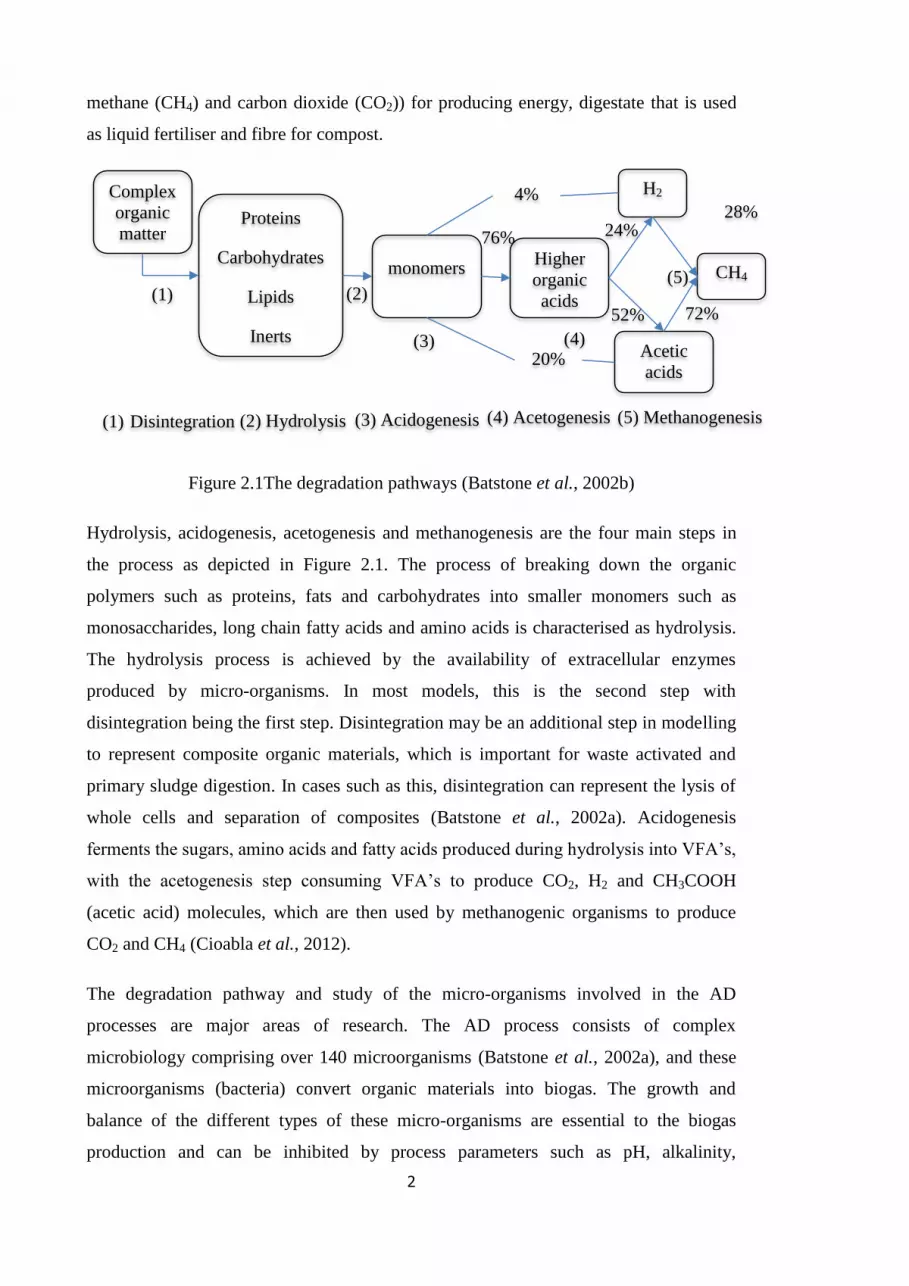
methane (CH4) and carbon dioxide (CO2)) for producing energy, digestate that is used
as liquid fertiliser and fibre for compost.
Figure 2.1The degradation pathways (Batstone et al., 2002b)
Hydrolysis, acidogenesis, acetogenesis and methanogenesis are the four main steps in
the process as depicted in Figure 2.1. The process of breaking down the organic
polymers such as proteins, fats and carbohydrates into smaller monomers such as
monosaccharides, long chain fatty acids and amino acids is characterised as hydrolysis.
The hydrolysis process is achieved by the availability of extracellular enzymes
produced by micro-organisms. In most models, this is the second step with
disintegration being the first step. Disintegration may be an additional step in modelling
to represent composite organic materials, which is important for waste activated and
primary sludge digestion. In cases such as this, disintegration can represent the lysis of
whole cells and separation of composites (Batstone et al., 2002a). Acidogenesis
ferments the sugars, amino acids and fatty acids produced during hydrolysis into VFA’s,
with the acetogenesis step consuming VFA’s to produce CO2, H2 and CH3COOH
(acetic acid) molecules, which are then used by methanogenic organisms to produce
CO2 and CH4 (Cioabla et al., 2012).
The degradation pathway and study of the micro-organisms involved in the AD
processes are major areas of research. The AD process consists of complex
microbiology comprising over 140 microorganisms (Batstone et al., 2002a), and these
microorganisms (bacteria) convert organic materials into biogas. The growth and
balance of the different types of these micro-organisms are essential to the biogas
production and can be inhibited by process parameters such as pH, alkalinity,
monomers
H2
Acetic
acids
Higher
organic
acids
CH4
24%
52% 72%
28% 4%
20%
76%
(2) Hydrolysis (4) Acetogenesis (5) Methanogenesis
Complex
organic
matter Proteins
Carbohydrates
Lipids
Inerts
(1) Disintegration (3) Acidogenesis
(1) (2)
(3) (4)
(5)

3
concentration of free ammonia and volatile fatty acids (VFA) and light and heavy
metals.
The AD system requires the acidogenesis and the methanogenesis stages to be balanced
to avoid inhibition of methanogenic bacteria. A key task in the control of the anaerobic
digestion (AD) process (automatic or otherwise), is the avoidance of inhibitory
conditions. Inhibition is any situation which prevents a specific microbial growth and
reproduction of the biomass that stabilises the sludge and forms biomethane. This is
usually caused by the presence of inhibitory chemicals (high acids) or biologicals
(hydrogen scavengers).
Inhibitors can be present in the AD process in the form of end products of feedstocks of
inorganic, organic substances or microbial reactions introduced into the anaerobic
digester. Anaerobic instability is the cause of the availability of various inhibitory
substances. Examples of inhibitory substances include CO2, ammonia and nitrogenous
matter such as proteins and urea. The degradation of nitrogenous organic matter leads
to ammonia production within the digester (Chen et al., 2008):
CaHbOcNd + 4a − b − 2c + 3d
4H2O
→ 4a + b − 2c − 3d
8CH4 +
4a − b + 2c + 3d
8CO2
+ dNH3
Equation
2.1
Inhibition has been shown to be difficult to quantify, due to the complex nature of the
digestion process mechanisms. These mechanism can be significantly affected by
antagonism (the suppression of some species of micro-organisms by others),
acclimation (adaptation to a new environment or a change to the old environment) and
or synergisms (micro-organisms acting together for mutual benefit e.g. syntrophy)
(Chen et al., 2008). An example of an antagonistic and or synergistic effects in ADs is
the impact of dual cations, where research has shown the effect of antagonism on
combining potassium and calcium increased significantly when compared to effect of
potassium alone (Kugelman and McCarty, 1965) .
The presence of inhibitory substances may cause shifts in the microbial population or
bacterial growth, with shifts in the microbial population indicated by a decrease in the
CH4 gas production rate, or by an accumulation of organic acids. Therefore by

4
measuring the gas production rate, the concentration of organic acids (VFAs), and or the
presence of chemicals known to cause inhibition, the AD process can be stabilised and
controlled.
The AD process is further exacerbated by complexities on a macroscopic level; the
three-phase (solid-liquid-gas) AD process involves both sequential and parallel reaction
pathways. The complexity and uncertainty in the dynamics of the micro-organisms
involved in the process make the process difficult to model. When considering a single
organism system, it is the case that no single kinetic model can describe the
complexities of that single organism. It is therefore a major task for scientists and
engineers to attempt to model multi-organism systems (Heinzle et al., 1993).
2.3 Modelling
The need for continuous improvement on existing AD process operations and
development of new processes with time, cost constraints and increase pressure on high
product quality and availability of sustainable products, have driven the technology
towards the use of model based process applications. Model building approaches still
require simple methods with ease of application, ‘the simpler the better’ (Foss et al.,
1998).
Mathematical models can serve as useful tools to deepen the understanding of complex
systems, and to facilitate operation and design of the process. If the behaviour of a
system can be predicted, the production of outputs can be optimised and process failure
can be prevented. However there is limited application of modelling approaches to AD
processes. This is due to the complexity of the process which requires extensive input
data, increased knowledge about the process dynamics and uncertainties within the
model. Therefore the AD process has traditionally been considered as a black box
system (Lidholm and Ossiansson, 2008).
There are various modelling approaches with differing ranges of accuracy and
complexity dependent on the purpose of the model. For control purposes a possible
complex, non-linear model with focus on the biochemical reactions with adequate
monitoring can aid in developing an understanding of the process. The control and
optimisation of AD systems requires an accurate dynamic model of the process.
However modelling of AD systems often results in high order nonlinear models with
several unknown parameters. This makes it difficult to control the process and therefore
various system identification techniques need to be applied to the AD process.

5
Modelling AD processes is an active research area with various review articles,
journals, thesis and book publications (Andrews and Graef, 1971; Lyberatos and
Skiadas, 1999; Dochain and Vanrolleghem, 2001; Batstone et al., 2002b; Zaher, 2005;
Saravanan and Sreekrishnan, 2006; Donoso-Bravo et al., 2011) which have been
conducted studies into modelling the anaerobic digestion process and thus only a
summary is given here.
Although extensive research into the microbiology of the process has been conducted,
there is still a lot of uncertainty surrounding this area. For example, there are knowledge
gaps such as the spatial distribution of individual organisms in flocs, granules and
biofilms (Jean-Philippe Steyer et al., 2006). This has a large effect on microbiological
reaction rates, and for this reason 'first principles' modelling is not currently suitable for
robust control. Given the importance of achieving a stable operating process,
robustness is the key objective of any control system, with performance being
important, but secondary for the improvement of ADs.
Andrews and his co-workers in 1974 worked on developing dynamic models for the
purpose of process control for AD (Andrews, 1974; Graef and Andrews, 1974a). To
date their models form the basis of most AD system models, and there has been little
development of newer models. Most attempts to identify the biological treatment
systems such as AD for the purpose of control, focus on the macroscopic fringes of the
process dynamics without much impact on the microscopic level (Beck, 1986).
In depth research into conversion mechanisms including cell decay, lysis and hydrolysis
indicated that hydrolysis of the dead particulate biomass is the rate limiting step and this
kinetically controls the overall process (Pavlostathis and Gossett, 1986), whilst more
recently methanogenesis has been shown to be the rate limiting step (Bowen et al.,
2014). However, it is evident that the rate limiting step varies for different conditions
(Appels et al., 2008). There are numerous models presented in the literature, from
simple Monod kinetics (Siegrist et al., 2002); first order models (Smith et al., 1988);
Andrews models (Graef and Andrews, 1974b); mass balance models (Bernard and
Bastin, 2005b); through to more advanced models (Polit et al., 2002; Ramirez et al.,
2009). However most of these models fail to accurately describe the digester dynamics,
as they do not assess both random and deterministic factors affecting the microbial
communities.
6
Various modelling complexities exist for AD system modelling; consideration of only
the acidogenesis and methanogenesis steps is the lowest level of modelling complexity.
Examples of these are given in Section 2.3.1. The highest level of complexity is
considering the disintegration and hydrolysis steps, the anaerobic digestion model no.1
(ADM1) model in Section 2.3.2 details this and middle model complexities include the
Siegrist model in Section 2.3.3.
2.3.1 Rate limiting step models
The rate limiting step is the slowest step which limits the overall process. Due to the
multistep characteristic of the process, initial mathematical modelling approaches
focused on the rate limiting step as this controlled the overall rate of the process.
Volatile fatty acids (VFA’s) were considered as the key parameter (Donoso-Bravo et
al., 2011) for modelling the rate limiting step. However as the rate limiting step changes
under different operating conditions, this resulted in different models as the rate limiting
step varies for different wastewater characteristics, loading rates, temperature and at
different stages of the process. Examples of the various modelling approaches focusing
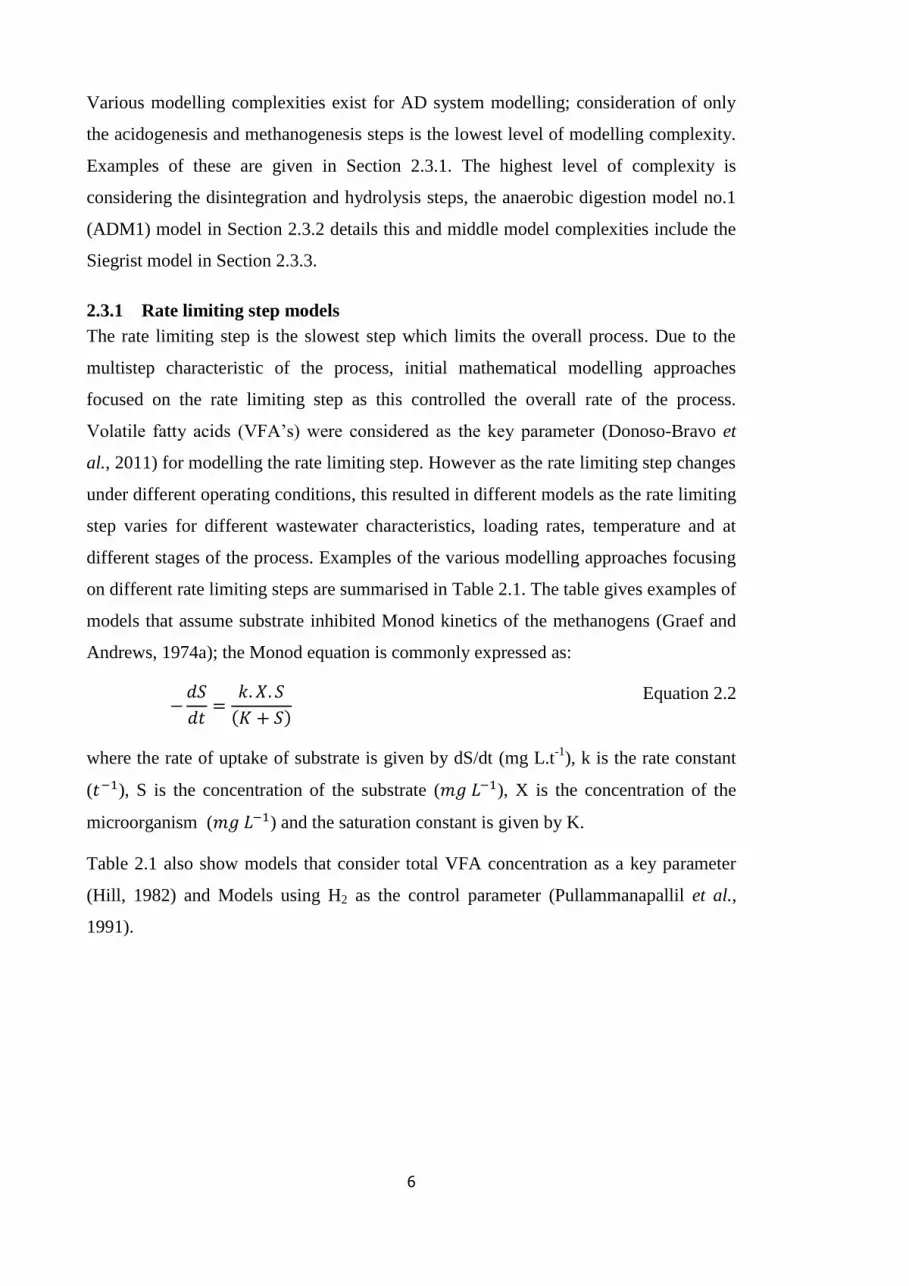
on different rate limiting steps are summarised in Table 2.1. The table gives examples of
models that assume substrate inhibited Monod kinetics of the methanogens (Graef and
Andrews, 1974a); the Monod equation is commonly expressed as:
−𝑑𝑆
𝑑𝑡=
𝑘. 𝑋. 𝑆
(𝐾 + 𝑆)
Equation 2.2
where the rate of uptake of substrate is given by dS/dt (mg L.t-1
), k is the rate constant
(𝑡−1), S is the concentration of the substrate (𝑚𝑔 𝐿−1), X is the concentration of the
microorganism (𝑚𝑔 𝐿−1) and the saturation constant is given by K.
Table 2.1 also show models that consider total VFA concentration as a key parameter
(Hill, 1982) and Models using H2 as the control parameter (Pullammanapallil et al.,
1991).

7
Table 2.1 Examples of Rate limiting step modelling
Model Bacteria group Rate limiting step
(Process)
Kinetic
Function
Graef and Andrews (Graef
and Andrews, 1974b)
Acetoclastic
methanogens
Methanogenesis Andrews
Hill (Hill, 1982) Acidogenic
bacteria
Acidogenesis Monod
based
Smith (Smith et al., 1988) Rapidly
degradable
biomass
Hydrolysis First order
Pullammanappallil
(Pullammanapallil et al.,
1991)
H2 utilising CH4
bacteria
Methanogenesis Monod
(pH)
2.3.2 The anaerobic digestion model no.1 (ADM1)
There are several AD models developed in recent years, however these mainly consider
a specific AD process or for a specific substrate; resulting in models that cannot be
compared or transferred to solve other problems. The ADM1 is the commonly used AD
model and consists of a complex multistep anaerobic process transformation model.
This first generalised AD model was created by the International Water Association
(IWA) task group for mathematical modelling of AD processes in 2002 (Batstone et
al.). The model provides a common basis for AD model development and validation
studies for ensuring more comparable results, and has been widely applied for
predictions of real AD system behaviour with a sufficient level of accuracy to be useful
in process development, optimisation, and control (Derbal et al., 2009; Mairet et al.,
2011). It is a standard benchmark for developing operational strategies and evaluating
process controllers for AD.
Although models have evolved to consider more process detail including more detailed
kinetics such as the ADM1 (Batstone et al., 2002b) model, they still fail to fully
represent the complex nature of the AD system. Thus the best-fit of a model from a set
of experimental data requires the optimum solution of the model parameter vector.

8
The first step to modelling is characterisation and fractionation of the influent as per the
model input variables. This is followed by model calibration by estimating the most
sensitive parameters of the model. Characterising the influent; this can be carried out in
ADM1 by various means including physical-chemical analyses, physical-chemical plus
online calibration, elemental analyses and input from another model. The ADM1 model
includes:
kinetics for disintegration of homogenous particles to carbohydrates, proteins
and lipids, followed by hydrolysis of these particles to sugars, amino acids and
fatty acids;
Inhibition functions of metabolic activity by ammonia, pH, acetate and H2, and
nitrogen limitation;
Description of gas-liquid transfer and ion association and dissociation;
32 dynamic concentration state variables, 26 state variables and 8 implicit
algebraic equations;
Exclusion of lactate formation, sulphate reduction, nitrate reduction, long chain
fatty acid inhibition, competitive uptake of H2 and CO2 and chemical and
biological precipitation.
As the model however does not include reduction of nitrate, precipitation, sulphur,
intermediate components of lactic acid and ethanol; there are also several modifications
and extensions of the ADM1 model which makes the model easier to implement for use
in process control. Such modifications models include the ADM1xp which incorporates
nitrogen (Wett et al., 2006), this model can be modified further depending on the
characteristics of the wastewater. Other common extensions of ADM1 include sulphate
reduction (Batstone et al., 2006) required for systems with high (greater than 0.002 mol
SO4 L-1
or 192 mg SO4 L-1
) sulphate levels in the effluent (Hinken et al., 2013).
Implementation of winery wastewater in ADM1 has been implemented by various
authors (Batstone et al., 2004; García-Diéguez et al., 2013), with ethanol as the main
Chemical Oxygen Demand (COD) of the winery wastewater and microbial diversity
modelling (Ramirez et al., 2009).
2.3.3 The Siegrist model
In 2002 Siegrist (Siegrist et al., 2002) published a slightly more simplified modelling
approach in comparison to ADM1. The exclusion of valerate and butyrate as state

9
variables was a key difference in this new model, with the hydrolysis rate modelled as a
single step process with first order kinetics with respect to the concentration of
particulate matter. The Siegrist model parameters are based on experiments, whereas the
ADM1 uses review consensus. The Siegrist model was calibrated with lab scale
experiments and validated with full-scale experiments. However the simplification in
Siegrist model came with ignoring several processes and including several assumptions.
The complex nature of the AD process means it cannot be modelled without several
simplifications, assumptions and disregarding various processes. Examples of these
include (1) the reactor is assumed to be completely mixed; (2) the liquid phase is
considered to be dilute and the volume is assumed to be constant; (3) the sludge
retention time (SRT) is equal to the hydraulic retention time (HRT); (4) fixed
stoichiometry in the microbial processes and (5) kla (volumetric mass-transfer
coefficient) value is only dependent on temperature (Lidholm and Ossiansson, 2008).
These various assumptions result in limitations in the model.
2.3.4 TELEMAC Anaerobic Model no. 2 (AM2)
The TELEMAC (TELEMonitoring and Advanced teleControl of high yield wastewater
treatment plants) Anaerobic Model no. 2 (AM2) focuses on Acidogenic and
Methanogenic reactions and models the methanogenesis of volatile fatty acids (Bernard
et al., 2001). AM2 accounts for the likely inhibitory effects of accumulated VFAs which
would result in reduced pH and accounts for this inhibition using Haldane kinetics:
𝑑𝑆
𝑑𝑡=
𝜇𝑚𝑎𝑥
𝑌
𝑆𝐵
𝐾𝑆 + 𝑆 + 𝑆 (𝑆𝐾1
⁄ )𝑛
Equation 2.3 (Lokshina et al., 2001)
Where µmax is the maximum specific growth rate (ℎ−1); 𝑆𝐵 is growth limiting substance
concentrations (𝑚𝑔 𝐿−1); 𝑛 is the Haldane index; 𝑌 is the growth yield (𝑚𝑔 𝐿−1); 𝐾𝑆 is
the half saturation coefficient and 𝐾1 is the inhibition constant. The AM2 is a mass
balance cascade structure model based on 70 day dynamical experiments covering a
wide operating range. The purpose of the model is to aid with the monitoring and
control of AD systems. This is achieved by ensuring the experiments cover a range of
experimental conditions and the validation step is performed with a wide set of transient
conditions.

10
2.3.5 Further model extensions
Table 2.2 Model Reduction Approaches
Model reduction approach Method Reduction
Bernard and Basin (Bernard and
Bastin, 2005b; Bernard and
Bastin, 2005a)
AMH1 Uses principal component analysis
(PCA) for reduction in the
biochemical complexity
Hassam (Hassam et al., 2012) Homotopy eigenvalue-state association to neglect
the slow dynamic aspect of the model
Gracia-Dieguez (García-Diéguez
et al., 2013)
PCA Extended PCA which can be used to
capture minimum of 2 reactions
Rodriguez (Rodriguez et al.,
2008)
PCA Uses PCA to determine the minimum
number of reactions of 3 reactions
Due to the underlying complexity and model assumptions in ADM1, there have been
several model modification and reduction approaches to aid with calibration and
increased use in control approaches. Model reduction methodologies include projection
methods and non-projection based methods. Projection based methods include Singular
Value Decomposition or orthogonal decomposition methods. These model reduction
methods aim to decrease simulation time, parameter estimation requirements, and
implementation workload. The Siegrist model can be deemed as a simplification of
ADM1 model as the model excludes butyrate and valerate components. Table 2.2
depicts examples of model reduction approaches for AD. The most detailed approach of
these is represented by Rodriguez and co-workers (Rodriguez et al., 2008), in this a
PCA technique is applied to experimental data from pilot scale AD, treating diluted
wine and compared with simulation data from the ADM1 model. The PCA technique is
used to determine the minimum number of reactions to be included in the model
structure to describe different percentage of data variability.
Since there are a large number of measured quality variables that are highly correlated
approaches use PCA to examine the relationships between different reaction pathways
as variables within the AD process data.
11
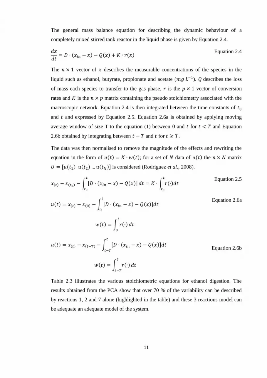
The general mass balance equation for describing the dynamic behaviour of a
completely mixed stirred tank reactor in the liquid phase is given by Equation 2.4.
𝑑𝑥
𝑑𝑡= 𝐷 ∙ (𝑥𝑖𝑛 − 𝑥) − 𝑄(𝑥) + 𝐾 ∙ 𝑟(𝑥)
Equation 2.4
The 𝑛 × 1 vector of 𝑥 describes the measurable concentrations of the species in the
liquid such as ethanol, butyrate, propionate and acetate (𝑚𝑔 𝐿−1). 𝑄 describes the loss
of mass each species to transfer to the gas phase, 𝑟 is the 𝑝 × 1 vector of conversion
rates and 𝐾 is the 𝑛 × 𝑝 matrix containing the pseudo stoichiometry associated with the
macroscopic network. Equation 2.4 is then integrated between the time constants of 𝑡0
and 𝑡 and expressed by Equation 2.5. Equation 2.6a is obtained by applying moving
average window of size T to the equation (1) between 0 and 𝑡 for 𝑡 < 𝑇 and Equation
2.6b obtained by integrating between 𝑡 − 𝑇 and 𝑡 for 𝑡 ≥ 𝑇.
The data was then normalised to remove the magnitude of the effects and rewriting the
equation in the form of 𝑢(𝑡) = 𝐾 ∙ 𝑤(𝑡); for a set of 𝑁 data of 𝑢(𝑡) the 𝑛 × 𝑁 matrix
𝑈 = [𝑢(𝑡1) 𝑢(𝑡2) … 𝑢(𝑡𝑁)] is considered (Rodriguez et al., 2008).
𝑥(𝑡) − 𝑥(𝑡0) − ∫ [𝐷 ∙ (𝑥𝑖𝑛 − 𝑥) − 𝑄(𝑥)]𝑡
𝑡0
𝑑𝑡 = 𝐾 ∙ ∫ 𝑟(∙)𝑑𝑡𝑡
𝑡0
Equation 2.5
𝑢(𝑡) = 𝑥(𝑡) − 𝑥(0) − ∫ [𝐷 ∙ (𝑥𝑖𝑛 − 𝑥) − 𝑄(𝑥)]𝑑𝑡𝑡
0
𝑤(𝑡) = ∫ 𝑟(∙)𝑡
0
𝑑𝑡
𝑢(𝑡) = 𝑥(𝑡) − 𝑥(𝑡−𝑇) − ∫ [𝐷 ∙ (𝑥𝑖𝑛 − 𝑥) − 𝑄(𝑥)]𝑑𝑡𝑡
𝑡−𝑇
𝑤(𝑡) = ∫ 𝑟(∙)𝑡
𝑡−𝑇
𝑑𝑡
Equation 2.6a
Equation 2.6b
Table 2.3 illustrates the various stoichiometric equations for ethanol digestion. The
results obtained from the PCA show that over 70 % of the variability can be described
by reactions 1, 2 and 7 alone (highlighted in the table) and these 3 reactions model can
be adequate an adequate model of the system.

12
Table 2.3 Stoichiometries of 9 considered reactions for digestion of ethanol (Rodriguez
et al., 2008)
Reaction EtOH BuH ProH AcH H2 CH4 CO2 H2O
R1. EtOH + H2O →
BuH + ProH + AcH +
H2
-1 0.100 0.042 0.737 1.758 -
0.758
R2. BuH + ProH + H2O
→ AcH + H2 + CO2
-1 -
0.419
2.419 3.257 0.419 -
2.838
R3. AcH → CH4 + CO2 -1 1 1
R4. H2 + CO2 → CH4 +
H2O
-1 0.25 -0.25 0.5
R5. BuH + H2O → AcH
+ H2
-1 2 2 -2
R6. ProH + H2O →
AcH + H2 + CO2
-1 1 3 1 -2
R7. H2 + AcH → CH4 +
CO2 + H2O
-1 -2 1.5 0.5 1
R8. EtOH + H2O →
AcH + H2
-1 1 2 -1
R9. EtOH + CO2 →
BuH + ProH + H2 +
H2O
-1 0.413 0.173 0.653 -
0.173
0.173
To summarise the current state of modelling approaches of AD process, the SWOT
analysis in Table 2.4 highlights the strengths, weaknesses, opportunities and threats. In
general the threats and weaknesses outweight the opportunities and strengths. These
have been the main reasons for limited modelling success with the AD process.
However with increasing focus, interest and funding of AD systems, from households to

13
businesses and governments it should enable the strengths and opportunities to
outweigh the weaknesses and threats due to knowledge and improved models.
Table 2.4 SWOT analysis of AD process modelling
Strengths
BBSRC ADNet scientific network
(Anaerobicdigestionnet.com, 2015)
Active research area with various publications;
with a range of simple models to advanced models
with benchmark models to compare new modelling
approaches
Established AD modelling community from
reputable institutions with models such as ADM1
Opportunities
Requirement for robust
models to understand the
underlying complexity of
the process
Opportunity for soft sensor
development for VFA and
H2
Threats
Lack of adequate instrumentation and monitoring
to generate process data that fully describes the
process
Lack of collaborations requiring expertise from
different subject areas including biologist, process
engineers, civil engineers
Weaknesses
Lack of robust models
explaining the complex
behaviour of the AD
process
Current models too large
and complex and difficult
to calibrate
2.4 AD technologies
AD systems can be configured in a number of ways:
1. Batch or continuous;
2. Plug flow or fully mixed;
3. Wet or dry;
4. Psychrophilic or Mesophilic or thermophilic;

14
5. Single stage or multi stage.
As an industrially focussed Engineering Doctorate, this literature survey reflects the
research requirements of the industry and as such there is greater emphasis on AD
technology in the wastewater treatment sector; which are generally configured as
continuous, fully mixed, wet systems. Key differences in these technologies are
variations of mesophilic or thermophilic (covered in detail in Section 2.5) and single
stage or multi stage.
Traditional AD systems are single stage operation where the sludge is fed into a single
digester for a period of time and through appropriate mixing and heating, biogas is
produced. These systems are generally mesophilic AD (MAD) systems and a series of
drivers have increased the complexities of AD technologies and resulted in increasing
need for a more robust system through the separation of the key stage of the process.
Process development for MAD systems began in the 1960’s where further
understanding of the need for heating, mixing and feeding systems became apparent
(Noone, 2006). At this stage the main driver was reduction of odour. The 70’s and 80’s
focused on separate processing inputs and their interactions and the drive during this
period was the EU directive on improving pathogen quality and bacteriological of
digestate sludge for land application (Noone, 2006). Current regulations and policies,
such as the climate change act (Climate Change Act, 2011), EU and UK targets for
energy from renewable sources and the Renewable Obligation Certificates (ROCs)
(ofgem, 2011b) system is driving the technology towards higher efficiencies, improved
yields and tighter regulations to make the technology more attractive from both a
technical and financial perspective.
Advanced anaerobic digestion (AAD) may be loosely defined as a treatment process
which improves the conversion of the organic material into biogas. AAD techniques are
typically multi-stage and require additional techniques to separate the different stages of
the process with pre-digestion techniques of thermal hydrolysis or enzymic hydrolysis
and improve substrate composition contact between the microorganisms and the organic
material. The two key steps in the digestion process are the acid forming stage
(acidogenesis), and the methane forming stage (methanogenesis). Different conditions
such as temperature and pH are required for the optimisation of these stages (Appels et
al., 2008). For example, there is a requirement for different optimum pH values for the
various phases of the digestion process. The hydrolysis and acidification phases require

15
lower pH values between 4.6 and 6.3, whereas the optimal pH range for the methane
formation stage is between 7.0 and 7.7. Separation of these stages enable optimisation
of each stage without hindrance on the other and therefore multi-stage AAD
technologies generally yield more biogas, higher digestate and biogas quality with
greater stability and robustness of the overall process than traditional single stage
processes.
The two leading AAD approaches are enzyme hydrolysis technology and thermal
hydrolysis. Other approaches include Ultrasound, Microsludge, OpenCEL, and Cell
Rupture. Thermal Hydrolysis Processes (THP) are typically large scale AD plants, with
15 plants in the UK, 14 in the rest of Europe and four in the rest of the world (CAMBI,
2011). There are over 200 AD systems in the UK using the enzymic hydrolysis
(Monsal, 2011). These are thus established and proven technologies with new plants
currently under construction for both technologies.
2.5 Temperature
AD generally operates in three temperature ranges of psychrophilic 4-20 °C, mesophilic
20-40°C and thermophilic 40-70°C (Batstone et al., 2002b). Mesophilic and
thermophilic systems are the normal operating temperature ranges with mesophilic
system being the most common and stable. The stability of mesophilic anaerobic
digestion (MAD) systems is a result of the wider diversity and robustness of bacteria to
grow at mesophilic temperatures and also that they are more adaptable to changes in
environmental conditions (Angelonidi and Smith, 2014).
Different optimum temperature values exist for different phases of the digestion
process, as methanogenic bacteria especially are very sensitive to temperature
fluctuations therefore temperature should be kept to within ±1˚C (Appels et al., 2008).
Local temperature variations may well indicate the presence of poor mixing, or dead
spots in the digester. Optimisation of the heat balance is important in improving the
digester operation and efficiency as a whole.
Temperature has a significant effect on biogas production. Budiyono and co-workers
(Budiyono et al., 2010) conducted experiments in a 400 ml digester using cattle manure.
The experiment was run at 38.5˚C and room temperature. Comparison of the average
gas production gave 5.8 ml gVS-1
per 1˚C increase in temperature. This value is
however based on the specific experimental set up and cannot be used generally as the
size of the digester and the feed affects conversion rates. Research has shown that in

16
general biogas production follows a sigmoid function as in a batch growth curve. Biogas
production is very slow at the beginning and end period of observation. A second report
by Alverez and Liden (Alvarez and Lidén, 2008) stated that by reducing the temperature
from 35˚ to 25˚C caused a 30 % reduction in volumetric biogas production rate was
observed for a Llama-cow-sheep manure bench top digestion process (Alvarez and
Lidén, 2008). However a 7˚C reduction from 25˚C to 18˚C caused a 51 % reduction in
the biogas volumetric production rate. This is expected as an increase in temperature
improves the kinetics in the system and hence increases the degradation rate. However
the results also showed high CH4 content which increased at low temperatures. The CH4
content in the biogas increased from 49.9 % to 61.1 % between 35˚C and 18˚C. This
counteracts with the fundamentals of a decrease in volumetric gas production rate. The
volumetric CH4 production rate was reduced from 2094 ml at 35˚C to 1676 ml CH4 per
day at 25 ˚C representing a reduction of 20 % (Alvarez and Lidén, 2008). A further
reduction of 47 % from 1676 to 894 ml CH4 d-1
was seen when the temperature was
reduced from 25 to 18˚C. Thus biogas production rate increases with decreasing CH4
composition for temperatures within the mesophilic digestion region of 30˚C to 35˚C.
An optimum temperature must be established at which high CH4 composition and
biogas yield are simultaneously optimised. The profitability of the anaerobic digestion
process is strongly affected by the percentage of CH4 present in the resulting biogas.
Any advanced control scheme must therefore optimise both CH4 and biogas yields.
2.6 Conclusions
AD technologies continue to be an attractive topic for scientists, engineers, industries
and governments, as they struggle to learn and understand the complexities of the
process and drive scientific and engineering development. They also align with
government drivers to reduce fossil fuels, find alternative energy sources and reduce
waste to landfills. The technology is experiencing major transitions through increased
focus on AD for combating climate change and biorefinery developments. The
dynamics of the process continue to increase with high uncertainties and increasing
complexities; the technology continues to develop with increase new industrial
processes.
Through conducting the literature survey it was found that instrumentation with respect
to sensors is a key limitation of industrial scale ADs. Various online sensors for key
variables exist at laboratory or experimental scale but are mainly offline analysis

17
methods and are not currently available on industrial scale application. The possible
reason for this may be due to cost, reliability, or market demand for example the need
for monitoring of the hydrolysis and fermentation stages which may require the
integration of spectroscopic sensors or soft sensors to efficiently predict important
parameters such as alkalinity and VFA. Efficient monitoring of these parameters is
deemed important for future research development (Ward et al., 2008). This issue has
led to the need for a detailed instrumentation review (summarised in Chapter 3) to
establish the gaps and opportunities in this area.
Following on from the instrumentation review, a vendor review was conducted to
identify the key technology players in the field with two questionnaires aiming to: (1)
gain input from the AD technology providing vendors and (2) understand the reasons
for the variation in the application of the various technologies to support the project.
The vendors included AD original equipment manufacturers (OEMs), pre-treatment
technology providers and various other suppliers for the process specifically for the
WWT market. This task was carried out to obtain input from the technology providers
on how their technologies could be integrated into the Perceptive AD master and the
AD process overall to meet the aims of the project. The key targeted technology
providers were Monsal and CAMBI. These two companies provide leading advanced
anaerobic digestion (AAD) technologies. Examples of their technologies are covered in
the benchmark study in Chapter 4. Involving the process designers was paramount to
the project as it allowed the opportunity to improve the process from the design level.
Response from the questionnaires through emailing and cold calling the vendors was
low and as a result, vendors were then targeted at several AD events and conferences.
The limited response received was inadequate to obtain insights from the vendors to
support the research and these are not presented in this thesis.

18

19
3 Instrumentation review
3.1 Introduction
This instrumentation review discusses the minimum and ideal instrumentation
requirements for an AD process. The economic and environmental benefits of biogas
production from an AD process are well understood and in recent years significant
technological developments for increasing the efficiency, yield, stability and robustness
of the system has increased the need for better monitoring of the process (Olsson et al.,
2005).
Current regulations and policies such as the climate change act (Climate Change Act,
2011), EU and UK targets for energy from renewable sources and the Renewable
Obligation Certificates (ROCs) (ofgem, 2011b) system are driving the need for higher
efficiencies, and improved biogas yields. These requirements make the investment in
control and monitoring technologies more attractive. This is supported by various
studies both in industry and academia. Due to the low energy efficiency for converting
biomass to electricity of only 13 % (Warthmann and Baier, 2013), there is an
opportunity to improve the efficiency and yield; monitoring and control will play a
crucial role.
The lack of process control handles, instrumentation, and developed control algorithms
have been addressed to some extent in the past 10 years (Boe et al., 2010; Palacio-Barco
et al., 2010; García-Diéguez et al., 2011; Cadena-Pereda et al., 2012; Vanwonterghem
et al., 2015). The current gap in instrumentation technology was the lack of availability
of rapid intermediate sensors to detect overloading conditions. To date there are a
limited number of sensors that can measure total or individual organic acids; with some
available on commercial production sites and others under development (Pind et al.,
2003).
There are on-going research projects in this area in both academia and industry, with
new types of instruments being commercialised frequently due to regulatory and
process improvement demands. There are wide varieties of instruments available at the
laboratory scale which is not yet applicable at an industrial scale. The gap between
laboratory and industrial scale instrumentation, control and automation is more
significant for AD than for most fields, as digestion at laboratory scale is much more
stable and easy to control than at an industrial scale (Horan, 2009).

20
An additional challenge has been dealing with the lack of reliability of existing sensors,
and the potential effect that they may have on a closed-loop control system and fault
detection algorithms have proven not to be satisfactorily reliable to detect faulty on-line
sensors. Robust control strategies based on on-line sensors include algorithms for
automated detection of faulty sensors. Sensor faults typically include drift, offset shift,
scaling shift, fixed value, complete failure, and calibration errors
Stability of the AD process may be indicated by biogas production rate, and effluent
VFA or effluent COD or TOC concentrations. When attempting to control parameters,
typically limited manipulated variables are available, with feed flow being the most
commonly used. Other manipulated variables include temperature, stripped gas,
agitation and mixing.
Plant wide optimisation needs to be taken into account for the implementation of any
control scheme. It is evident that energy balance is an important plant performance
indicator, particularly where CHP operation is utilised for the downstream process
(Horan, 2009). For this reason, the monitoring of the energy used and produced by the
various heat and power units is necessary. Flow and temperature probes are reliable and
well established within the industry and in such situations where instrumentation is
unavailable; it should be implemented to enhance energy utilisation.
3.2 Instrumentation technology providers
A common aphorism in the field of control instrumentation is “To measure is to know”.
In the past, the availability of sensors was a key obstacle for control and automation of
WwTPs. Measurements for treatment systems were mainly limited to pH, flows and
dissolved oxygen (DO). This situation has improved over the last 10 years, and
currently sensors for biochemical oxygen demand (BOD), COD, ammonia, nitrate,
nitrite and phosphate are now available for on-line monitoring of wastewater treatment.
The book entitled “Instrumentation, Control and Automation in Wastewater Systems”
gives a good account of developments in this area up to 2005 (Olsson et al., 2005). Key
conclusions with respect to the state of instrumentation, control and optimisation up to
2005 were:
Limited usage of sensors for closed loop control approaches
Improved ease of data collection and visualisation through the adoption of
supervisory control and data acquisition (SCADA) systems

21
Process or plant wide control and optimisation approaches are new areas for
development
50 % of control loops surveyed were found to be in manual mode
Lack of on-line sensors no longer deemed as the main limitation for on-line
control, process flexibility recognised as a greater limitation.
Table 3.1 Examples of technology providers for AD systems
Company Instrument Details
Bioprocess
Control Ltd
Biogas OptimizerTM (Products
| Bioprocess Control, 2016)
A SCADA solution which allows
process diagnosis, decision support
and optimisation; and Automated
Methane Potential Test System
(AMPTS) system
SCAN Spectrolyser, pHlyser,
ammolyser, chlorilyser, and
turbilyser (SCAN, 2011)
Spectral probes, ion selective probes,
electrochemical sensors, optical
sensors
Geotech GA3000 and GA4000 (Products
Archive - Geotechnical
Instruments (UK) Ltd, 2016)
Simple fixed position biogas analyser
and laser diode analyser for highly
accurate CH4 analysis
Endress
Hauser
Flow, level, pressure (Level,
flow, pressure, temperature
measurement |
Endress+Hauser, 2016)
Data logging and digital
communications
Hitech
Instruments
GIR5000 ('GIR5000 series -
Biogas & Landfill analysers -
Multiparameter analysers for
biogas applications,' 2016)
Designed specifically for biogas
applications and measures CH4, CO2,
and O2 or H2S
AppliTek Anasense (AppliTek, 2009) Monitors VFA, bicarbonate and
alkalinity

22
Various companies have portfolios of instrumentation specifically to address the needs
of the water industry. Although the state of instrumentation for process units such as
activated sludge plants (ASPs) has improved considerably, there is still a lack of
suitable instrumentation for ADs. Table 3.1 depicts different technology providers for
AD systems; such as the spectrolyserTM which is specifically designed for WwTP
(SCAN, 2011). This SCAN spectrometer probe has proven to be reliable for the online
monitoring of BOD, COD, Total Soluble Solids (TSS), pH, nitrate and temperature
(O'Brien et al., 2011) for the treated effluent stream of an ASPs. The multi parameter
probe uses UV-Vis spectrometry over the range 220-720 nm or 220-390 nm and can be
mounted in the media or in a flow cell with automatic cleaning using compressed air
(SCAN, 2011). Instrumentation such as this has made some ASP control solution
implementations possible yielding, improved process efficiency.
Another example of on-line instrumentation developed specifically for monitoring AD
systems is the Anasense® from AppliTek. An example of the Anasense Control Unit is
shown in Table 3.2. This system is used in the TELEMAC supervision system to
monitor VFA, bicarbonate and alkalinity. The TELEMAC project is aimed at bringing
new methodologies from the IT and science sectors to water treatment, and compares a
group composed of leading scientist and engineers offering an advanced remote
management system for anaerobic WwTPs which do not benefit from a local expert in
wastewater treatment. The TELEMAC system involved new sensors for improved
monitoring of the process dynamics and with automatic controllers that stabilise the
treatment plant (Bernard et al., 2004).

23
Table 3.2 Example of instrumentation control units
CH4 analyser from Nova
Analytical Systems Inc. (Nova
analytical systems, 2010).
Anasense from
AppliTek NV
(AppliTek, 2009)
pH or Redox (ORP) &
Conductivity analyser from ABB
(pH / ORP transmitters -
Analytical Measurement | ABB,
2016)
The HK microwave dry solids measurement system shown in Figure 3.2 is
manufactured in Germany by Harrer and Kassen and distributed by Process
Instrumentation UK Ltd. This analyser is typically commissioned for a cost < £10,000
and the instrument is capable of measuring % DS within the range 0 % to 40 % DS. A
low power oscillator in the microwave measuring instrument is used to generate an
electromagnetic wave which is then transmitted into the sludge via an antenna. The
wave is transmitted through the dielectric properties of the sludge. This is received by a
second antenna and the phase delay and power level of the wave received are
proportional to the concentration of the product (density) or the dry solids (UK, 2011).
Figure 3.1 The HK microwave dry solids measurement system (UK, 2011)

24
The ISO 15839:2003 standard is the most complete protocol for sensor characterisation
in water quality for on-line sensors and analyser equipment for water specifications as
well as performance tests (Iso.org, 2015). Most of the instruments detailed in the survey
conformed to this standard. Sensor characteristics covered by the standard include
performance metrics of range, linearity, accuracy, drift and speed of response.
The provision of more standard measurements such as temperature, pressure, liquid
level, and flowrates are not considered in this survey, as such instruments are readily
available, with state of the art technology found on many plants. Physico-chemical
measurements such as pH, conductivity, redox, CH4, H2S, H2, CO2 and bio-chemical
measurements of BOD and TOC are readily available with state of art technologies.
Measurements of suspended solids, bicarbonate alkalinity, digester gas and UV
absorption have application only in certain areas. Measurements systems which require
further development work include sludge morphology, calorimetry, COD and VFA.
An important precursor step in the development of robust control solutions to ensure
enhanced AD operation is the development of robust sensors and analysers. Challenges
limiting the success of control strategies in AD typically include uncertainty in the
process kinetics and uncertainty in the input and output flows and concentrations. The
availability of reliable sensors can help overcome these limitations. Sensors can be
categorised into two groups (1) reliable simple sensors for operator support and
regulatory control of the process and (2) advanced sensors tools for auditing,
optimisation, modelling activities (Vanrolleghem and Lee, 2003).
3.3 Sensors and instruments
This section provides a discussion on instrumentation in the solid, liquid and gas phases
of the AD process. Variables can be measured in the gas or liquid phase. Liquid phase
measurements include VFAs, pH, COD, dissolved H2 and alkalinity, whilst gas phase
measurements consist of flowrates, and composition of species such as CH4, H2S, H2,
CO2 and siloxanes (Ward et al., 2008). Sensors for physical parameters such as flowrate
are of importance in the process. Gas flowrate measurements are provided using
differential pressure techniques, turbine sensors or magnetic flow sensors.
Figure 3.1 illustrates the various parameters measured in the solids phase as well as
liquid and gas phases.
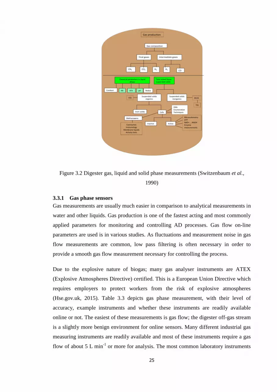
25
Figure 3.2 Digester gas, liquid and solid phase measurements (Switzenbaum et al.,
1990)
3.3.1 Gas phase sensors
Gas measurements are usually much easier in comparison to analytical measurements in
water and other liquids. Gas production is one of the fastest acting and most commonly
applied parameters for monitoring and controlling AD processes. Gas flow on-line
parameters are used is in various studies. As fluctuations and measurement noise in gas
flow measurements are common, low pass filtering is often necessary in order to
provide a smooth gas flow measurement necessary for controlling the process.
Due to the explosive nature of biogas; many gas analyser instruments are ATEX
(Explosive Atmospheres Directive) certified. This is a European Union Directive which
requires employers to protect workers from the risk of explosive atmospheres
(Hse.gov.uk, 2015). Table 3.3 depicts gas phase measurement, with their level of
accuracy, example instruments and whether these instruments are readily available
online or not. The easiest of these measurements is gas flow; the digester off-gas stream
is a slightly more benign environment for online sensors. Many different industrial gas
measuring instruments are readily available and most of these instruments require a gas
flow of about 5 L min-1
or more for analysis. The most common laboratory instruments
Gas production
n CO2
Gas composition
Intermediate gases Final gases
CH4
H2
S
CO
H2
VFA
Chemical parameters in liquid phase
Conduct pH
Alk
Redox
Suspended solids organics
Inert solids
Coenzymes Immunology
Membrane liquids Activity tests
Methanogens
Total mixed liquor suspended solids
Suspended solids inorganics
Active
Inactive
Cells
Microcalometry ATP NAD+…..NADH Enzyme measurements
DNA Enumeration Techniques
MLSS
TSS
VSS

26
are volumetric displacement and can measure gas flow at very low concentrations. The
measured gas flow signal can be affected by noise, usually due to the effects of
foaming. This noise typically requires online filtering to provide a useable signal (Pind
et al., 2003).
Biogas flow monitoring systems are readily available and widely applied in industry and
the accuracy of these instruments is affected by temperature values due to dilution of
water vapour in the gas with increased temperature which can increase from 8 % at
35oC to 17 % at 55
oC. Prices range considerably between portable devices and fixed
point or wall mounted modular devices and continuous process monitoring; with the
Gas Data GFM416 biogas analyser costing around £3200.

27
Table 3.3 Gas phase measurements
Technology Types or
Method
Ranges or Level of
Accuracy
Reliability
and Cost
On-line or Process
Dynamics
Examples
Gas
flow
Volumetric displacement
instruments, thermal
dispersion devices, orifices
plates, pilot tubes and turbine
meters
Range: 0-500 Nl min-1
. and
± 0.5 % repeatability, 5
L·min–1-0.1mL·min–
1(Guwy et al., 1995)
£3000-
5000
Speed of response
typically 30 seconds
Geotech-GA3000, HiTech-
GIR5000, Gas Data-GFM416
(Products Archive -
Geotechnical Instruments
(UK) Ltd, 2016)
CH4
and
CO2
Volumetric displacement
measurement, GC, IR
adsorption analysis methods
CH4 0-60 % and CO2 10-
50 % of total gas.
£800-1500 Readily available
both lab and
industrial scale
LI-COR, CEA CH4,
Servomex Ir1520
H2 Mercury-mercuric oxide
detector cell (0.01ppm),
thermistor metal conductivity
0-4 % range typically by
volume
£350-500 None found
H2S Measure H levels using
electronic sensors or gas
measurements,
electrochemical sensors
In concentrations between
0-50 ppm in gas produced
£200-500 GC and FT-IR
analysis, applied to
6 sites (Arnold and
Kajolinna, 2010)
None found
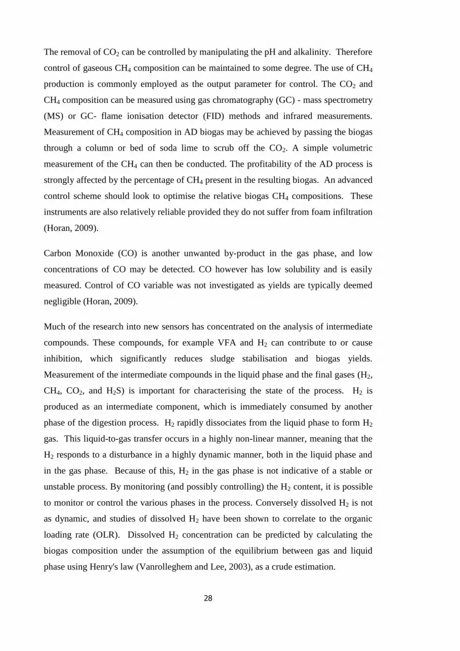
28
The removal of CO2 can be controlled by manipulating the pH and alkalinity. Therefore
control of gaseous CH4 composition can be maintained to some degree. The use of CH4
production is commonly employed as the output parameter for control. The CO2 and
CH4 composition can be measured using gas chromatography (GC) - mass spectrometry
(MS) or GC- flame ionisation detector (FID) methods and infrared measurements.
Measurement of CH4 composition in AD biogas may be achieved by passing the biogas
through a column or bed of soda lime to scrub off the CO2. A simple volumetric
measurement of the CH4 can then be conducted. The profitability of the AD process is
strongly affected by the percentage of CH4 present in the resulting biogas. An advanced
control scheme should look to optimise the relative biogas CH4 compositions. These
instruments are also relatively reliable provided they do not suffer from foam infiltration
(Horan, 2009).
Carbon Monoxide (CO) is another unwanted by-product in the gas phase, and low
concentrations of CO may be detected. CO however has low solubility and is easily
measured. Control of CO variable was not investigated as yields are typically deemed
negligible (Horan, 2009).
Much of the research into new sensors has concentrated on the analysis of intermediate
compounds. These compounds, for example VFA and H2 can contribute to or cause
inhibition, which significantly reduces sludge stabilisation and biogas yields.
Measurement of the intermediate compounds in the liquid phase and the final gases (H2,
CH4, CO2, and H2S) is important for characterising the state of the process. H2 is
produced as an intermediate component, which is immediately consumed by another
phase of the digestion process. H2 rapidly dissociates from the liquid phase to form H2
gas. This liquid-to-gas transfer occurs in a highly non-linear manner, meaning that the
H2 responds to a disturbance in a highly dynamic manner, both in the liquid phase and
in the gas phase. Because of this, H2 in the gas phase is not indicative of a stable or
unstable process. By monitoring (and possibly controlling) the H2 content, it is possible
to monitor or control the various phases in the process. Conversely dissolved H2 is not
as dynamic, and studies of dissolved H2 have been shown to correlate to the organic
loading rate (OLR). Dissolved H2 concentration can be predicted by calculating the
biogas composition under the assumption of the equilibrium between gas and liquid
phase using Henry's law (Vanrolleghem and Lee, 2003), as a crude estimation.

29
3.3.2 Liquid phase sensors
Monitoring of the intermediate chemical species that are created within the digester
vessel and then immediately consumed within the same vessel (or an immediate
downstream vessel) can provide key information on microbial activity. The
intermediates produced are degraded from soluble and insoluble proteins, carbohydrates
and lipids. Monitoring of these intermediates is carried out in the liquid phase, within
the digester vessel itself. Instrumentation for the monitoring of the biological
intermediates such as VFA and bicarbonate alkalinity is an active research area. Soft
sensors for VFA and alkalinity have been developed to enable better monitoring of the
process. Finally the analysis of the fermentation stage of the digestion process is
achieved through techniques such as photometric cuvette tests, ion chromatography, or
titration methods.
VFAs are fatty acids with a carbon chain of less than six. These are deemed to be the
most important intermediates in the process. The conversion of VFAs to CH4 and CO2
is conducted through the acetogenesis and methanogens stages. The monitoring of the
VFA composition gives important information about the state of these stages. As the
composition of the feedstock entering the digester can vary greatly, the general
interpretation of the VFA concentration can become highly problematic. For example,
an increasing VFA content may be due to a change in the feedstock, or alternatively it
may be due to a change in the microbial balance between the different stages. These
two different causes require diametrically opposite control actions, therefore VFA
monitoring at multiple points in the process is important for optimal control of the AD
process. The most important drawback to fulfil automatic control of VFAs is the lack of
on-line measurement devices, and the potentially high cost of those instruments that are
available.
Current methods for VFA measurement include distillation, calorimetry, GC and
various titration techniques. Of these approaches the titrimetric methods are considered
to be more rapid, simplest and most cost effective. Most of these assume that VFAs are
mainly composed of acetic acid (Bouvier et al., 2002). In the literature several
publications have reported the on-line monitoring of VFA’s through titrimetric methods
(Bouvier et al., 2002; Feitkenhauer et al., 2002).
30
Table 3.4 Liquid phase measurements
Technology Types or
Method
Ranges or Level of
Accuracy
Reliability or
Cost
On-line or Process Dynamics Examples
VFA Distillation, calorimetry,
chromatography and
titration techniques; GC,
HPLC, GCMS, MS
technologies.
VFA accumulation
reflects a kinetic
uncoupling between
acid producers and
consumers
£12000-20000 HSGC (Kanokwan et al., 2007),
FT-IR spectrometer as an on-line
sensor (J. P Steyer et al., 2002),
Multi-syringe and multi-pumping
combined system;
spectroflourimeter (Palacio-Barco
et al., 2010)
Anasense®
(AppliTek,
2009) Ammonia Ion selective, and
electrochemical based
sensors such as ion
selective electrode (ISE)
, colorimetric
100–1100 mg-N · L–
1; Colorimetric range:
0-10 mg/l, ISE range:
0-20000 mg/l,
Accuracy: 2 % or
0.015mg/l
£12000-20000 Anasense®
(AppliTek,
2009), SCAN:
Ammolyser
(SCAN, 2011)
H2 Amperometric probe (50
nM), H2 or air fuel cell
(80 nM), mass
spectrometry, coiled
silicone tubing in the
reactor.
Typically an
estimate from
H2 gas. Not
readily
available yet
Available on lab scale and
estimation mechanism for
industrial application based on H2
gas
None found
BOD Spectrometer: measure
optical spectra from 200
to 750 nm directly in
liquid
Not an usual
parameter for AD
None found Lab scale in-house developed
biosensor (Liu et al., 2004)
Carbolyser
(SCAN, 2011)
COD or
TOC
Spectrometer measure
optical spectra from 200
to 750 nm directly in
liquid
COD: 0-1500 mg L-1
O2 and 2 % accuracy.
TOC: 0-10000 ppm
and accuracy: 2-3%
£25000-£30000 FT-IR spectrometer as an on-line
sensor
Carbolyser
(SCAN, 2011)
Alkalinity,
PA, TA
Total buffer capacity 1000-3000 mg L-1
typically
None found FT-IR spectrometer as an on-line
sensor
Anasense®
(AppliTek,
2009)

31
Off-line measurements of VFAs for verifying the state of the biomass within the AD has
been applied in control studies. In these studies, the control algorithm has been based
on other measured on-line parameters of inorganic chemical components, such as redox
potential, ammonia, pH, and alkalinity. Another approach has been VFA estimation
using a modified nitrate sensor for measuring nitrate reduction through a denitrifying
organism immersed in partially digested feedstock’s in an excess of nitrates. Measuring
nitrate reduction through titration is proportional to the organic carbon (Ward et al.,
2008). Titrimetric methods can also be applied for the analysis of total and partial
alkalinity.
VFAs are formed during the acidogenesis and acetogenesis stage. A stable efficient
fermentation process yields VFA component (acetic, propionic, butyrate etc.) values
between 500 to 3000 mg L-1
as the equivalent amount of acetic acid. There is
equilibrium between the production of acid by hydrolysis and acid degradation by
methanation. An acid concentration above 10000 mg L -1
results in pH drop usually
below 7 and results in a reduction in CH4 concentration. This parameter could
potentially be monitored and controlled using the Anasense instrument.
The pH level in the digester is a particularly important parameter for monitoring and
control. In general the ideal range of pH is between 6.6 and 7.6. If the pH is
particularly low, then the methanogenic bacteria essential to the final stage of CH4
production will be inhibited. Currently there are a wide range of sensors available for
the measurement of pH, however many pH probe electrodes are prone to electrode
poisoning due to the harsh environments in the digestion process. The hydrogen
sulphide (H2S) concentration present in the sludge causes electrode poisoning to most
pH monitoring instrumentation. The Hach Lange pHD sc digital differential electrode
for pH and redox measurement is designed to overcome this problem. The reference
system of the pHD sc electrode does not come into contact with the fluid that is being
measured and avoids the problem of electrode poisoning.
The measurement of carbohydrate levels in the digester vessel is also considered.
Substrate carbohydrates may be in either soluble or insoluble form. The measurement
of soluble carbohydrate is comparatively much easier, using methods such as high
performance liquid chromatography (HPLC) which may be applied on-line. In
comparison insoluble carbohydrates require complicated pre-treatment methods, after
which they can be measured using HPLC, colorimetric methods or GCMS. Because of

32
the pre-treatment requirements, on-line measurements are not possible. Even for offline
lab measurements, the costs for these measurements are sufficiently high and hence
these measurements are only conducted on a small scale. Currently there is no direct on-
line measurement of the composition of either H2S or CH4 in the liquid phase
(Vanrolleghem and Lee, 2003). Any future developments in the measurements of these
parameters may yield new potential control strategies.
Temperature sensing probes are relatively cheap and reliable, and the digester vessel
can be instrumented with a number of these at various positions both radially and
axially around the circumference of the vessel. Local temperature variations may well
indicate the presence of poor mixing, or dead spots in the digester. Temperature probes
should also be mounted in the hot water circuit entering the digester, and possibly on the
biogas streams leaving the digester. This would allow the online calculation of the
digester heat balance. Optimising the heat balance is essential to optimising the digester
operation as a whole.
The use of gas flow measurement as an on-line parameter is found in numerous studies.
This is regarded as a key monitoring parameter (in conjunction with the sludge feed
rate), as it is a relatively fast indicator of changes in the microbial population.
Soluble H2 is an intermediate species which is both produced and immediately
consumed in the AD process. Gaseous H2 concentration may be measured using a
mercury-mercuric oxide detector cell; an exhale H2 monitor; or palladium metal oxide
semiconductors (Pind et al., 2003). H2 has a very short relaxation time as shown in
Table 3.5 and the content in the gas phase could be between 20-30 ppm to 400-600 ppm
which makes measurements much easier in the gas phase.
Table 3.5 Theoretical relaxation times for some AD parameters (Switzenbaum et al.,
1990)
Substrate H2 Glucose CO2 Acetate Propionate CH4
Relaxation time 15 seconds 3 minutes 1 hour 2 hours 4 hours 2 days

33
H2S is produced as a result of the degradation of sulphide containing compounds such
as proteins in small quantities. H2S forms a small proportion of the overall biogas
composition.
3.3.3 Solid phase sensors
For the AD process, the 'solid phase' refers to solids carried in liquid suspension, either
in the feedstock, digestate, or in the main body of the digester vessels. Solid
measurements are usually conducted on feedstock prior to entering the digester and then
post digestion, so as to ensure that the instruments can be accessed for maintenance
purposes. The main purpose of measuring the solids before and after digestion is to
evaluate the percentage solids reduction, which indicates the level of microbial activity
in the digester. Accurate measurement of the solid component properties is more
difficult compared to gas or liquid measurements. Solid phase parameters for
measurements include percentage dry solids (% DS), cell enumeration,
deoxyribonucleic acid (DNA) sequencing, protein content, bacterial lipids, adenosine
tri-phosphate (ATP), enzyme activities, methanogenic activity measurement, micro-
calorimetry, co-enzymes, C1-carriers of methanogens and immunology of methanogens.
In general these parameters are not often used for automatic control as these are usually
measured off-line with long analysis periods and complex systems for measurement
(Moletta, 1998). Laboratory analyses for the characterisation of bacteria or the organic
compounds are mostly carried out for research purposes and typically not an actively
monitored process parameter.
One of the newer sensor types is near-infrared spectroscopy (NIRS), which is used in a
variety of industries for classifying or predicting the characteristics of complex media
and bulk solid materials. NIRS is a non-destructive optical technique, which produces a
spectrum as its output, as such NIRS requires a multivariate technique such as partial
least squares (PLS) regression to map the spectral output to one or more measured
physical parameters. NIRS has the advantage of being able to measure several
parameters simultaneously providing a calibration model is prepared for the parameters
of interest. The need for a calibration model is a drawback for the NIRS technique, as
each type of waste may require its own calibration model and a biochemical methane
potential (BMP) test may still be required to obtain the reference value. NIRS has been
used to monitor ADs mostly for determining VFA content and BMP.

34
Table 3.6 Solid phase measurements
Technology Types or
Method
Ranges or Level of
Accuracy
Reliability
and Cost
On-line or Process
Dynamics
Examples
Total organic
carbon (TOC)
Spectrometer: measure
optical spectra from 200 to
750 nm directly in liquid
Range: 0-10000 ppm;
Accuracy: 2-3 %
Average
price £25000
FT-IR spectrometer as an
on-line sensor
SCAN:
Carbolyser
VOC Spectrometer: measure
optical spectra from 200 to
750 nm directly in liquid
Not an usual parameter for
AD
None found GC and FT-IR analysis,
applied to 6 sites (Arnold
and Kajolinna, 2010)
None found
Indirect
measurement of
organic matter
Assessment of VS and total
solids (TS)
Not a usual parameter for
AD, calculation on the inlet
feed to digester, varies
dependent on feed.
None found None found None found

35
One key variable for the digestion process is the % DS fed into the digester. Typically
this parameter is measured off-line, and these spot sample results are then used to adjust
the sludge dewatering process accordingly. The optimum solid content obtained for
biogas production is in the range of 7 to 9 percentage dry solids (% DS) (Balsam, 2002).
This is the amount of solids in sludge, which contain organic matter of proteins,
carbohydrates, fats, nutrients. Due to the function of water in the digester, the total
solids (TS) content will directly correspond to water content. Water content is an
important parameter as it enables the movement and growth of bacteria, facilitating the
dissolution and transport of nutrients and contributes to the metabolic reactions as most
of these are dependent on the hydrophobicity of the organic material. Water can also
reduce the limitation on mass transfer of non-homogenous or particulate substrate
(Budiyono et al., 2010). % DS information may be used to estimate the organic loading
to the digester. The organic loading rate (OLR) is a key parameter for the operation of
the digester. An OLR greater than 3 kg VS (m3.d
-1) may lead to overloading of the
digester which will in turn require a reduction in the sludge feed rate to allow the
digester to recover.
Online DS meters for the sludge feed stream are available, and are relatively reliable.
These sensors are designed to work with sludge dry solids contents in the range 0 % to
10 %. This sensor information may be used to estimate the organic loading of the
digester which is a key parameter for operating the digester; a loading rate above 3 kg
VS (m3.d
-1) may lead to overloading of the digester which will in-turn require a
reduction in the sludge feed rate in order to allow the digester to recover.
In the UK, the use of treated digestate sludge as an agricultural fertiliser is governed by
the 'Safe Sludge Matrix' (SSM). This is a set of rules governing what type of crops that
different sludge can be applied to. A 'conventionally treated sludge' is one in which at
least 99 % of pathogens have been removed. An 'enhanced treated sludge' is one in
which at least 99.9999 % of pathogens have been removed. Table 3.7 shows the UK
Safe Sludge Matrix (Chambers et al., 2001). The matrix sets out the types of crop
groups which may be treated with conventional, enhanced or untreated sludge.
The main driver for determining how a digester is operating is ensuring that the digested
sludge is compliant with sludge stabilisation requirements. Beyond the requirements for
pathogen reduction there is no other direct specification for digestate quality in general
use. As it is deemed to be a waste product, digestate is excluded from the main farm
quality assurance scheme and this is the main obstacle for applying digestate use on

36
agricultural land (Booth, 2009). This will inevitably change due to increased regulations
and the move towards selling digestate as a product.
Table 3.7 The safe sludge matrix (Chambers et al., 2001)
Crop group Untreated
sludges
Conventionally treated sludges Enhanced
treated sludges
Fruit ×
× √
√
√
√
10 month
harvest
interval
applies
Salads ×
× (30 month harvest interval
applies)
Vegetables ×
× (12 month harvest interval
applies)
Horticulture ×
×
Combinables
and animal feed
crops
× √ √
Grass and forage
(grazed)
× × (deep injected
or ploughed
down only)
3 week no
grazing and
harvest
interval
applies
√ 3 week no
grazing and
harvest
interval
applies Grass and forage
(harvested)
× √ (no grazing in
season of
application)
√
Regulations such as these articulated in the Code of Good Practices (CoGP) and SSM
are used for sludge stabilisation in the UK. Treatment processes for sludge are managed
by the principles of hazard analysis and critical control point (HACCP) management.
HACCP applies risk based management and control procedures to manage and reduce
potential risks to human health and the environment. The HACCP approach is adopted
and applied to sludge treatment, to ensure that the microbiological requirements set out
in the SSM are achieved and that the appropriate quality assurance and risk

37
management and reduction procedures are in place. This ensures that if the digestate is
being spread on agricultural land, it complies with the relevant microbiological
standards (Davis et al., 2010).
The SSM however does not include specific sludge quality indices. In an attempt to
remedy this, the waste resources action program (WRAP) created an industry
specification, the Publicly Available Specification (PAS 110) (WRAP, 2010) which
producers use to verify that digestate produced is of consistent quality and fit for
purpose. Some of the parameters from the PAS 110 guidelines include limits for toxic
elements such as copper, zinc and lead; limits for digestate stability characteristics such
as VFA and residual biomass potential as well as declaration of nutrient characteristics
of total nitrogen, phosphorus and potassium (NPK) values (WRAP, 2010). In March
2011, the Andigestion plant in Devon became the first AD plant to achieve digestate
certification and the site is approved under the Biofertiliser Certification Scheme (BCS).
BCS was built on from PAS 110 and offers a tool for classifying digestate (Organic-
farmers-and-Growers, 2011).
To comply with these guidelines, adequate instrumentation for the measurement and
monitoring specified parameters may be required in the near future, with a key
challenge being the ability to reliably and accurately measure these parameters.
Currently composition can be analysed within the laboratory as opposed to online in the
digester and hence soft sensors may be developed to as surrogate measurements.
3.3.4 Software sensors
There are limitations in the availability of reliable on-line sensor instruments for those
parameters discussed previously. It is possible that these limitations may be overcome
through the development and deployment of software-based sensors (also known as
'inferential sensors' or 'soft sensors').
A software sensor associates a hardware sensor and an estimation algorithm (software)
to provide on-line estimate of an un-measurable variable (Chéruy, 1997) and this will be
discussed in detail in Chapter 7. The key to a successful software sensor is to make use
of multiple instances of cheap, reliable, and easy to maintain sensors (such as flows,
temperatures and pressures) together with an appropriate multivariate model or
algorithm, in order to estimate some hard-to-measure parameter in real-time.
Development of software sensors for AD is an active research area, with new models
38
and techniques being published frequently. There are many common models used in
developing soft or inferential sensors.
The phenomenological or model driven approach, which is commonly based on first
principle models, describes the underlying physical and chemical background of the
process. As these models are usually based on the ideal steady-state of the process
(which for AD is largely unknown), this makes their use as the basis for soft sensors in
AD problematic.
The data driven approach employs a range of data analysis techniques including
univariate or multivariate statistical analysis, artificial neural network and fuzzy models,
and rely on a historical record of past behaviour of a particular process to estimate
future behaviour. These are more popular as they are perceived to describe the real
process condition as the data used is measured within the processing plant.
There is an increasing need for model based estimators to reliably predict costly or
unavailable measurements on the basis of related but less expensive on-line sensor
values (Theilliol et al., 2003). An example of such a system is a model which calculates
the risk of foaming due to microbiological causes. As causes of foaming in AD are not
in complete agreement; this model has encapsulated invaluable empirical knowledge of
key factors, with organic loading rate (OLR) and filamentous microorganisms present in
the activated sludge system, as the inputs to the model. This case study was used to
evaluate the performance of the model used in the IWA Benchmark Simulation Model
No. 2 as a framework (Alex et al., 2008a). Simulation results for one open loop
configuration and two close loop control strategies proved the usefulness of this
approach for the estimation of the risk of foaming in AD’s (Dalmau et al.).
Currently the use of soft sensors on industrial scale processes is limited, mainly due to
the difficulty in developing robust models and in validating cause sensor information. It
is common practice to analyse samples off-line to compare results to the soft sensor
value to ensure that the reliability of the soft sensor.
The development of a software sensor typically requires an intensive laboratory
sampling campaign to develop the sensor, as well as periodic lab samples to validate the
software sensor values, and to provide 'bias correction' for unmeasured drifts in values.

39
As such, the software sensor approach would be more suitable for parameters which are
frequently measured, such as VFA or pathogen levels in digestate.
3.3.5 Sensor requirements for advanced control
As a result of this instrumentation review and the benchmark study in Chapter 5,
‘minimum’, ‘essential’ and ‘nice to have’ instrumentation requirements for considering
the implementation of any advanced control scheme are summarised in Table 3.8.
Table 3.8 Summary of instrumentation
Minimum Essential ‘nice to have’
Input
Pressure or level
measurements
% DS Chemical
composition
Feed flowrate TOC COD
Process
state
Temperature VFA Redox potential
pH Bicarbonate alkalinity,
alkalinity, total alkalinity
Ammonia
Intermediate gases
of H2 and CO
Output Biogas composition
(CO2, CH4 and H2S)
Heating and cooling
elements
Biogas flowrate VS
The minimum instrumentation requirements are readily available easy to measure
instruments which provide basic monitoring of the input, process state and output
parameters of the system. In addition to the minimum level of instrumentation, essential
instrumentation requirement includes sensors that characterise the digester environment
and give some indication of the microorganism activity, such as VFA, or bicarbonate
alkalinity. Additionally, sensors mounted prior to the AD to give the characteristic of
the quality of incoming sludge (such as % DS, bicarbonate alkalinity) would enable a

40
reduction in the uncertainty in the process. Within the context of an advanced control
scheme, manipulated variables could be adjusted in response to these measured
disturbances, in order to meet control strategies. As these new sensor types become
readily available, there is still a barrier of reliability, accuracy, and cost to overcome and
gain widespread usage in monitoring, control and optimisation of AD systems. This is
considered as the main hurdle for new instruments developed for bicarbonate alkalinity
and VFA. Sensors that are non-essential or ‘nice to have’ for control include ammonium
which exists in a pH dependent equilibrium with ammonia. An increase in the pH shifts
the equilibrium to favour ammonia. Ammonia is toxic to bacteria and acts as an
inhibitor when present in the process. However ammonia inhibition is only more
evident in protein rich feedstocks (Wiese and Ralf, 2007). Online monitoring of
ammonia content ensures a trouble free operation and ammonia probes are relatively
commonplace in activated sludge plant operation, with the same probes being applied to
digester sludge streams.
As biogas production requires anaerobic environment better yields, redox potential is
recommended to be below 330 mV. Feedstocks containing oxygen, nitrate groups and
sulphate extensively affect the redox potential and thus the pH, as such redox potential
is also recommended as ‘nice to have’ measurement.
Choosing an ideal sensor for application on existing or new plants need to be conducted
with great care. The recommendation for minimum, 'essential' instruments listed in table
3.8 are provided at any site considered for a pilot study.
Conclusions
AD is not a new technology, however due to the biological nature of the process, the
relatively harsh environment and the lack of robust validation methods for new
instruments, there is a general lack of available instrumentation for measuring the
biological and chemical state in the digester vessel. In addition, gaps in the core
knowledge of the underlying mechanisms involved make it difficult to quantify the need
for a specific instrument. Continuous developments are ongoing with respect to more
robust, sophisticated sensors in order to provide insight into the major uncertainties and
disturbances in the AD process. However there is a requirement for further development
by both academics and industrialists to improve the reliability of new instruments and
also the applicability of the information provided by these instruments for automated

41
monitoring and control systems. Clearly the benefit of applying new instrumentation is
improved monitoring and better operator understanding with more flexibility with
respect to the operation of the process. Additionally, new sensor data provides
information to further understand and improve the process. In most cases, biological
and chemical laboratory data such as alkalinity and VFA concentrations is used as
'backup information' to better inform daily operation, rather than for closed loop
optimisation. Use of such data for developing soft sensor models may provide frequent
prediction of VFA to improve the daily operation and control of the process. Hence,
information from such a sensor should be collected, interpreted, and acted upon in real-
time, within the framework of an advanced control system to optimise the process.
Recent developments from Bioprocess Control (with the Automatic Methane Potential
Test System), AppliTek (with the Anasense instrument) and others are paving the way
for online monitoring and control of AD systems. As these instruments have not
achieved widespread industrial usage, it is difficult to assess the reliability and accuracy
of them. For example, the Anasense® instrument has been validated on both pilot scale
and industrial scale by its developers. Their conclusion was that the system requires
further developments in order to improve its robustness, especially in the presence of
highly charged cations (Molina et al., 2004). This demonstrates that robustness is a
significant hurdle for some newly developed sensors.
The recommended essential sensors for AD control shown in Table 3.8; beyond this, the
minimum level of instrumentation for attempting advanced control in AD should
include (1) some means of measuring the disturbances being applied to the process; the
most significant disturbances being the rate, concentration, and nature of the feedstock.
Whilst the flow is commonly measured, the concentration and the composition often are
not measured. Installation of online dry solids meters for this purpose is recommended.
Additionally it may be possible to characterise the composition of the feed by accurately
tracking the relative proportions of primary, secondary and co-digestion feedstocks
being applied to the digester. In addition to this, measuring the ammonia content of the
feedstock with an ammonia probe may yield considerable benefits. (2) Some means of
measuring and or characterising the biological or chemical conditions within the
digester itself. By monitoring and controlling such measurements, the stability of the
digester can be maintained. Of the available sensors, pH and ammonia probes appear to
offer the best chance of producing repeatable and reliable information. The Anasense®

42
probe for measuring VFA's is an exciting development, but it may not be sufficiently
robust to allow for industrial process control. Furthermore if such an instrument is
trialed, then there should be a parallel development of a software based sensor, which
may prove to be considerably more reliable. Chapter 7 volatile solids soft sensor
development aims to increase the level of monitoring on the process and further
development of soft sensors can help improve the level of monitoring significantly.
Additional improvements can be gained by closely working with instrumentation
providers such as Geotech to develop more robust reliable instruments. As part of this
research, Perceptive Engineering Ltd engaged with Geotech to trial the Capilex VFA
instrument. Trials with the instrument were not conducted during the period of this
thesis; however increase collaborations between AD processers, Universities,
instrumentation and technology providers can improve the development of increase
robust instruments and the level of monitoring on the AD system.

43
4 Methodology
4.1 Introduction
Traditionally AD systems have been constructed as large civil engineering projects and
the need for monitoring, control and optimisation has been a low priority and as such
retrofitting new instrumentation can be difficult. New AD systems currently being built
are however more automated and involve input from cross disciplinary fields. Although
some of the systems involved in this study are fairly new, there is still a limited degree
of instrumentation and monitoring. Therefore, there is a need to use techniques to
extract as much information from the process as possible to improve the monitoring and
control of these complex systems. There are a considerable number of approaches
available and the information extraction techniques applied here include principal
component analysis (PCA), partial least squares (PLS), recursive least squares (RLS)
neural networks (NN), model predictive control (MPC), quadratic programming (QP)
and various data pre-processing strategies.
Bioprocesses in general are inherently difficult to control, but there has been a range of
successful approaches reported in the pharmaceutical and food industries. In common
with other bioprocesses, the characteristic of the AD bioprocess, which exhibits varying
dynamics and complexity, makes it difficult to monitor and control.
Data driven methods for developing soft sensors and process models for process
monitoring and control through multivariate statistical analysis are widely applied and
well established techniques. Within the AD community however, soft sensor application
on industrial processes are limited. The industries perception of the AD process is
changing and moving away from the AD process being a waste reduction process to a
manufacturing process with high value output products, for which there is increasing
need to improve the process through enhanced instrumentation and control.
The overall aim of the research presented in this thesis is to design an integrated
monitoring and optimal control system for the supervisory operation of anaerobic
digesters (AD). There are several sub-objectives required to achieve this aim:
1. Quantification of the baseline performance of existing plants;
2. Review of existing instrumentation;
3. Modelling of the AD plant behaviour, with the emphasis on biogas production,
digester stability and quality attributes of digestate and biogas;

44
4. Soft sensor development to improve monitoring and measurement systems as
required;
5. Assessment of the challenges of a generic AD controller and or optimiser;
6. Optimal integration of AD systems within wastewater treatment works (WwTW
s);
7. Assessing the opportunities for an advanced controller on AD systems;
8. Prototype development of controller or optimiser system fulfilling the aims of
the user requirement specification (URS);
9. Controller performance evaluation and system improvement.
This will form a complete engineering cycle of specification, design, modelling,
implementation and testing as depicted in Figure 4.1. The specification stage involves
quantification of the baseline performance, review of existing instrumentation and
assessment of the challenges of a generic controller. The design phase will involve
using the results of the specification stage to formulate the URS developed through the
benchmark analysis (Chapter 5). Modelling for the controller and soft sensors constitute
the modelling step. Prototype development of the advanced controller will form the
development stage which will then be tested and evaluated through integration of the
system on WwTW and controller performance evaluation.
Quantification of baseline performance of existing plants has enabled key strengths,
weaknesses, opportunities and threats affecting the project aim to be identified.
Example of strengths include: (1) identification of several commonalities within the
results from the four main WwTWs such as variability in certain measurements makes it
easier to transfer models from one plant to the next, (2) significant bottlenecks identified
for each site and (3) quick fix money saving solutions identified, giving greater value to
the overall project. Several opportunities were also identified along with various
weaknesses and threats and these are summarised in Table 5.6. One of the key
weaknesses found was lack of instrumentation which resulted in the benchmarked
systems not being fully evaluated on a physiochemical and biological scale. This also
posed a greater threat as without adequate instrumentation on the process to monitor key
parameters; the aims of control cannot be achieved. This led to the need to fully review
instrumentation on the AD process. Soft sensor application on the AD process was
identified as a key means of overcoming the instrumentation limitation on the process,
while at the same time recognising that soft sensors are also reliant on instrumentation.
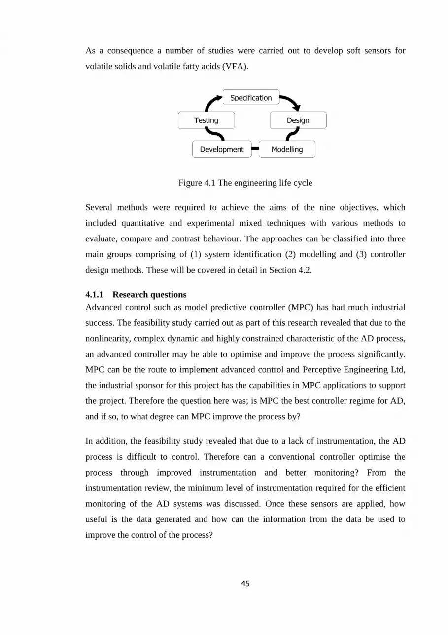
45
As a consequence a number of studies were carried out to develop soft sensors for
volatile solids and volatile fatty acids (VFA).
Figure 4.1 The engineering life cycle
Several methods were required to achieve the aims of the nine objectives, which
included quantitative and experimental mixed techniques with various methods to
evaluate, compare and contrast behaviour. The approaches can be classified into three
main groups comprising of (1) system identification (2) modelling and (3) controller
design methods. These will be covered in detail in Section 4.2.
4.1.1 Research questions
Advanced control such as model predictive controller (MPC) has had much industrial
success. The feasibility study carried out as part of this research revealed that due to the
nonlinearity, complex dynamic and highly constrained characteristic of the AD process,
an advanced controller may be able to optimise and improve the process significantly.
MPC can be the route to implement advanced control and Perceptive Engineering Ltd,
the industrial sponsor for this project has the capabilities in MPC applications to support
the project. Therefore the question here was; is MPC the best controller regime for AD,
and if so, to what degree can MPC improve the process by?
In addition, the feasibility study revealed that due to a lack of instrumentation, the AD
process is difficult to control. Therefore can a conventional controller optimise the
process through improved instrumentation and better monitoring? From the
instrumentation review, the minimum level of instrumentation required for the efficient
monitoring of the AD systems was discussed. Once these sensors are applied, how
useful is the data generated and how can the information from the data be used to
improve the control of the process?
Specification
Design
Development
Testing
Modelling

46
There are questions associated with the overall aim of the project, concerning the
different technologies and complexities of AD systems. How transferrable are the
findings from the benchmark, inventory control and soft sensor studies applied to
different AD systems so far? Is the same level of instrumentation required for the
different AD technologies? What are the similarities between AD systems and what are
the significant differences? If there was a different population of microorganisms would
the same parameters need to be monitored and controlled?
The process of developing the research started with the conceptual phase of formulating
the ideas into a realistic research design. Following successful application of advanced
control solutions on wastewater treatment processes (WwTP) (activated sludge
processes in particular) by Perceptive Engineering Ltd (O'Brien et al., 2011); market
research analysis was conducted considering the opportunities for advanced control on
ADs. The consortium was formed and the aims of the feasibility studies were then set.
Through the initial literature review, the scope and significance of the problem was
understood and the gaps in the current state of art were identified.
4.1.2 Research design
Figure 4.2 Knowledge extraction from data pyramid (Xue Zhang Wang, 1999)
The overall research aim of this project is to evaluate whether an advanced controller
such as MPC can improve the AD process. Determining whether the aims have been
achieved will require three fold technical justifications of assessing the improvements
observed through MPC; the financial case to ensure that the payback period for
Raw data
Data
Information
Knowledge
Rules
Volume
Value
47
installing the controller is within the time frame set by the consortium and the
application is ethical, sustainable and transferrable to other AD systems. Critical to the
success of this is instrumentation, access to industrial AD processes and knowledgeable
engineers.
Figure 4.2 demonstrates the stages of data mining from which information and
knowledge are extracted from raw data. This is the underlying theme throughout the
various studies undertaken within this project. Data can exist in any form with no
significance, knowledge or information beyond its existence. Thus raw data may exist in
large volumes whilst yielding little known value or useful transparent information that
can easily be understood. Selection of raw data and pre-processing provides data that
can be transformed into information. Rules and decision making tasks can then be
performed from interpretation of the information into knowledge, enabling data to be
transformed from a data rich source into information rich output moving up the
pyramid.
From the lower levels of the pyramid upwards; the value in knowledge increases whilst
the volume of data decreases. On industrial AD processes hundreds of parameters may
be measured, of these only a limited number may be of interest for operating the
process. Managers and high level decision makers may monitor or require knowledge
from only a couple of key performance indicators (KPI’s) to make decisions about the
process. Thus the knowledge of the process increases whilst the volume of data
decreases. Within this project, large volumes of data were collected during the
feasibility stage to gather information about the various processes. This was used as
knowledge for building models from which rules such as controller settings, ranges for
operating parameters and measures of performance indicators could be set to evaluate
the system behaviour. In terms of the modelling aspects of this project, at one site data
from approximately 800 signals were obtained and of these only 50 signals were
deemed useful for assessing the status of the process. For the soft sensor study only 8
process data signals were selected from which the final model only used two signals
which related to the output parameter. Thus the use of low volume data to obtain
knowledge from an initial high volume of data is a common theme within this research.

48
4.1.3 Overview of applied methods in thesis
A range of techniques are applied to fulfil the needs of the studies within the project.
These will be covered in detail within the different sections of the thesis and a summary
is given here. The various methods include: system identification; methodology for soft
sensor development; benchmarking of industrial processes; controller design; and
optimiser design. The five steps to be followed for building models, making use of the
methods and achieving the aims of this project are:
1. Selection of raw data (raw process data for benchmark, DoE and perturbed or
excited plant data);
2. Data pre-processing;
3. Knowledge interpretation (model building);
4. Information transformation (soft sensor development);
5. Decision making from established rules (advanced controller application).
Selection of raw data is a critical point in the overall research to avoid the concept of
‘rubbish in, rubbish out’ outcome of process data modelling. The nature of the results
generated from the various modelling techniques will depend heavily on the quality of
data used for the modelling. Following selection of useful data, inadequate data pre-
processing can result in unreliable models. Knowledge interpretation from these models
is also essential and requires deep understanding of the AD system.
Figure 4.3 Levels of methods
In moving towards improved operational objectives it is necessary to consider data
generation, system identification, modelling and control and optimisation methods.
Data
generation
methods
Historical process
data
Simulation data
Data generation
through DoE
System
Identification
methods
Principal
component
analysis (PCA)
Correlation
analysis
Recursive least
squares
Modelling
methods
Partial least
squares (PLS)
Neural networks
(NN)
Control and
optimisation
methods
Quadratic
programming
(QP)
Model predictive
control (MPC)

49
These are shown in Figure 4.3. Data generation methods applied here include the use of
historical process data, simulated and excited or DoE generated process data. Due to the
large operational difference in laboratory scale AD and industrial ADs, laboratory
assessments are not considered for this research. Historical process data is first used, as
years of data are freely available. Simulations are also used to generate data, as these are
cost effective ways of obtaining data; however they are not as accurate representation of
industrial ADs due to modelling difficulties arising with bioprocesses.
System identification is the approach of building mathematical models of dynamic
systems based on observed data from the system (Lennart, 1999). System identification
forms a major part of this research. Once data has been generated, a series of system
identification methods can be applied to gain knowledge about the process. This broad
area covers many methods including linear, nonlinear, parametric, nonparametric,
hybrid structures. The simplest approach to system identification is impulse response
identification, where the impulse needs to be large enough to enable the response to be
greater than the noise within the system (Dimitry, 2005).
4.2 Modelling
Science is generally based on inference of models from observations and studies on
their properties. The models become the paradigms, hypothesis, laws of nature and
interpretation of the true system. The model thus is the concept of how variables relate
to each other when they interact with the system. As true representation of the system
cannot be achieved through models; models are evaluated on their usefulness rather than
truth (Appels et al., 2008). The system characteristics that model approximates can be
defined by:
Linearity - obeying the principles of superposition with additive and scaling
properties;
Causality - if output depends only on the present and or past values), stability (if
the system does not diverge;
Memory - whether the system depends on the present value alone or can it
depend on the past and future values too;
Time invariant - lack of time dependency on the system, such that the system’s
response to a given input does not depend on the time the input is applied.

50
These system properties must be considered when building the model. The model
building has three basic entities; these include (1) the data set, (2) the model structure
and (3) model identification methods. This can consist of many steps and thus within
this research the model building approaches cover the stages of problem statement,
defining the modelling environment, conceptual modelling, model representation,
implementation, verification, initialisation, validation, documentation and model
application.
4.2.1 Model identification techniques
The control and optimisation of AD systems require an accurate dynamic model of the
process. However modelling of AD systems often result in high order nonlinear models
with several unknown parameters.
Least squares (LS) is the most popular cost function for parameter identification in AD
models. LS generally describe the approach of solving an overdetermined system of
equations through an approximation. The aim of the method is to minimise the sum of
the squares of the residuals rather than solve the inexactly specified system (Cleve,
2004). The LS estimation can be constructed in the simple form of
𝒚 = 𝐀𝐱 + 𝒗 Equation 4.1
Where y constitutes sensor measurement, x is the estimator, v is the unknown noise or
measurement error and the 𝒾th row of A characterises 𝒾th sensor. The estimation is
conducted by choosing �̂� that can minimise ∥ 𝐴�̂� − 𝑦 ∥. This is the deviation between
what is actually observed by (y) and what can be observed if = �̂� , with no noise where
𝑣 = 0. The LS estimation is thus �̂� = (𝐴𝑇𝐴)−1𝐴𝑇𝑦. This gives the maximum
likelihood estimation of the parameters (Stephen, 2008).
With regards to a control solution for the AD process, it is useful to have a model of the
AD system available online that updates as the process changes. Methods for solving
such problems are usually called adaptive methods. Identification techniques for such
systems are termed recursive identification methods (Lennart, 1999). Recursive least
squares (RLS) is a recursive variant which improves the efficiency of LS algorithm. The
RLS algorithm works by moving through a time history dataset and continually
updating model coefficients as it passes through the dataset. The algorithm uses the
covariance matrix weight factor, which determines how quickly the model coefficients

51
are changed. Recursive identification tools are common for handling systems with
varying dynamics as in the case of the AD process. A new parameter set can be
estimated for each observation. While the update of parameters may be attractive, there
are a number of shortcomings including:
Numerical instability and sensitivity to outliers;
Sensitivity of RLS to the initial conditions of the algorithm;
Slow tracking capability for time varying parameters (Jiang and Zhang, 2004).
However RLS is still a popular approach for online parameter estimation applications
and as such the method is used widely in this research.
4.2.2 Soft sensor based methods
The behaviour of a process is indicated by the state of the process and the process inputs
that impact on it. The states of many secondary ‘explanatory’ variables reflect the states
of the primary variables. Secondary variables are variables whose values can be
explained by changes in other variables such as primary variables. With the abundance
of computer aided tools available, the concept of inferential or software measurement is
well defined and inferential model building techniques are commonly applied. However
while the concepts are common, there are still key design factors to consider. These
include the characteristic of the data, the need for robust pre-processing techniques to
carefully remove noise and outliers within the data. The selection of the correct
secondary outputs and inputs for model building, in combination with process
knowledge is essential in generating a model that is both mathematically applicable and
sound from an engineering perspective. The model must then be tested for reliability
based on how the estimator deals with measurement problems, delays, infrequent
sampling and the irregular return of information.
Process stability is a measure of the consistency of the process with respect to process
characteristics; a stable process behaves consistently over time. In the digestion process
the different environmental condition requirement for the acid and methane forming
bacteria is the major cause of instability in the process, this is followed by inhibition and
foaming. Due to the large instability in AD processes, it is common in practice to
construct digesters larger than the optimal size to reduce the impact of instability. This
is expensive with respect to construction, operation and maintenance. By monitoring

52
key variables in the process, instability can be reduced, but to do so requires knowledge
of the causes of instability.
Digester instability can be a result of hydraulic, organic and toxic overloading (Graef
and Andrews, 1974a). Hydraulic overloading is a result of an organisms inability to
reproduce before being washed out due to the reduction in the residence time. The
residence time is defined as the reactor volume divided by the influent sludge flowrate.
Organic overloading is a result of build-up of volatile acids which can cause inhibition
to methanogenic organisms. Toxic overloading is generally caused by feeding the
digester with materials which can kill methanogenic organisms. These may include
heavy metals, ammonia, detergents, organic chemicals and cations. Thus monitoring of
key parameters that can provide indication of instability in the digester can improve the
monitoring to avoid digester failures.
Table 4.1 Examples of modelling techniques on AD systems
Measurements Estimation methods Uncertainty Reference
CH4 Non-linear regression
with the Marquardt-
Levenberg algorithm
Covariance matrix-
FIM
Lokshina et
al. (2001)
TSS, VSS, Biogas,
COD, VFA and gas
composition
Least squares criterion Confidence region
and linear
confidence interval
Kalfas et al.
(2006)
Biogas Gradient search
technique
Confidence region Batstone et
al. (2009)
Various methods have been used for software or inferential sensor developments. Table
4.1 lists examples of AD system modelling techniques for estimating some useful AD
parameters, and some of these techniques will be explored in detail in Chapter 7.
4.2.3 Control approaches on AD processes
The term advanced control can be misleading in its meaning. In its early days it was
taken to mean any alternative control to the traditional three term (proportional, integral,

53
derivative) controller. However it can describe the practice of using elements from
various disciplines that include control engineering, decision theory, artificial
intelligence, statistics, signal processing, hardware and software engineering.
The three phase AD process involves sequential and parallel reaction pathways. The
complexity and uncertainty in the dynamics of the microorganisms involved in the
process make it difficult to model. In comparing multi-organism systems to single
organism systems, it is widely accepted that no single kinetic model can describe all the
complexities of the single organism system; it is therefore a major task for scientists and
engineers to model multi organism systems. Initial attempts to model the AD process
concentrated on the rate limiting step, but this varies for different conditions. In general
hydrolysis is the rate limiting step. Most of these models in literature (Appels et al.,
2008) are very specific and steady state in nature. These are simple models, and most
tend to fail to accurately describe the digester dynamics. The aims of these models are
generally to achieve the following:
Estimation of process states such as reactor volume, biogas production, its
compositions and retention time etc. for determining the performance of a
specific system;
Allow sensitivity analysis to be conducted for various process parameters;
Allow assessment of model differences and knowledge of where the process can
be improved;
Whole plant optimisation capability providing understanding of how the
digestion process can affect the downstream processes (Appels et al., 2008).
Within the AD process, the acid and methane forming microorganisms differ in
physiology, nutritional needs, growth kinetics and sensitivity to environmental
conditions. Maintaining the balance between these microorganisms is crucial to gain
stability of the whole process and this is generally the primary cause of digester
instability (Jean-Philippe Steyer et al., 2006). The complexities of the AD process
increases the number of control objectives, thus from the feasibility results undertaken
so far, an ideal control scheme for the process should aim to have the following
objectives:
1. Pathogen reduction to meet compliance;

54
2. Optimise biogas production;
3. Optimise CH4 composition;
4. Optimise the multiple attributes of digestate quality;
5. Improve the energy balance of the AD process and with other processes on the
site to optimise efficient use energy;
6. Align gas production with ‘triad’ periods to gain maximum revenue;
7. Align combine heat and power (CHP) unit with AD for optimum energy
production;
8. Limit inventory disturbance to the upstream and downstream process (several
hierarchal control objectives);
9. Control of temperature to a minimum variation;
10. Control of % DS to enable optimum organic loading rate (OLR) feed without
overloading digester;
11. Control of retention time to meet compliance and optimise throughput;
12. Control of feed flow with minimum variability to improve stability;
13. Odour reduction control;
14. Foam reduction control.
Some of these objectives conflict with each another and require sophisticated control
systems to achieve the best balance of the objectives. There is thus a requirement for a
complex multi objective controller. An ideal controller will therefore need to meet or
balance all these objectives or as many as possible. Most industrial AD control
applications mainly include simple PI and PID controllers to control temperature and
levels, however there are examples of pilot and laboratory scale artificial neural
networks (ANN), fuzzy logic, linear and nonlinear model based control (Pind et al.,
2003) on industrial AD systems and these tend to be single objective in nature. This

55
limitation of a single input, single output control strategy, often linear in form is
insufficient to handle a complex process such as AD.
The AD process has large unknown number of microorganisms in a population from
various sources and different processing units. The lack of complete knowledge of the
system environment and direct cause and effect relationships of the various parameters
make the task of achieving the goals of the project complicated. Varying AD
configurations, system characteristics, structures (due to physical, geographical and
legislative factors) and input characteristics limit the use of generic models to achieve
the aims of control for AD systems (Wahab et al., 2007). These have resulted in varying
range of control strategies and structures applied.
4.3 Advanced control
Process control in bioprocesses aims to influence the individual behaviour of the
different living cells in the digester by controlling their extracellular environment
(Boudreau and McMillan, 2007). The extracellular environmental state condition can be
determined by process variables. These process variables must be measured or inferred
from other measurements to enable them to be controlled. Process control aims to
transfer variability from process output to the process inputs subject to measurement
resolution, noise, loop dead time, repeatability and controller tuning (Boudreau and
McMillan, 2007).
4.3.1 Model predictive control
MPC also known as receding horizon control (RHC), dynamic matrix control (DMC)
and generalised predictive control (GPC) consists of control algorithms which
numerically solve an optimisation problem at each step (Dimitry, 2005). The algorithm
used in this research is based on the minimisation of the cost function:
𝐽 = ∑ [𝑒𝑖+1𝑃𝑒𝑖+1𝑇 + ∆𝑢𝑖𝑄∆𝑢𝑖
𝑇]𝑁𝑖 = 1 Equation 4.2
Where the weighting matrices are given by 𝑃 and 𝑄 over the horizon, N. ∆𝑢 is the
vector of the current and future control moves subject to constraints, 𝑒 is the vector of
the setpoint tracking errors, 𝑖 is the sample point.
MPC models provide the exponential and ramping time response for deviations about
operating points. MPC involves the operation of multivariable controllers under process
constraints (Sandoz et al., 2000). These constraints may be ‘hard’ constraints of

56
manipulated variable (MV) minimum and maximum limits, incremental move limits, as
well as ‘soft’ constraints such as the controlled variable (CV) minimum and maximum
limits. This makes the MPC controller ideal for constraint optimisation problems found
in the AD process. There are several methods available to manage such constraints,
such as long range (LR), quadratic programming (QP) and a combination of these two;
long range QP (LRQP).
The PerceptiveAPC (Perceptive Engineering Ltd, 2012) MPC solution uses the QP
constraint management method. The QP solver aims to optimise by minimising or
maximising a quadratic function of multivariable form, subject to linear equality and
inequality constraints.
QP can be incorporated into MPC for constraint linear control, which is the general,
conventional approach. General objectives of an MPC includes (i) input, output
constraints violation prevention (ii) driving CVs and MVs to steady state optimal
values, (iii) prevention of excessive moves of MVs and controlling the plant when
signals and actuators fail. There are therefore trade-offs and approximations to translate
these objectives into a mathematical problem statement for defining the character of the
controller. Different possible solutions exist for defining this and therefore naturally
there are several MPC control formulations. Perceptive Engineering Ltd has several
model forms incorporated into PerceptiveAPC which include finite impulse response
(FIR), autoregressive with exogenous inputs (ARX), linear and nonlinear modelling
with NN. The steady state and dynamic optimisation objective is achieved with QP and
output horizon through finite horizon. Most MPC products are based on linear empirical
models, however nonlinear processes such as the AD can be represented by a discrete
time nonlinear model such that:
𝒙𝒌+𝟏 = 𝒇(𝒙𝒌, 𝒖𝒌), 𝒙𝒌 ∈ 𝕩, 𝒖𝒌 ∈ 𝕌, Equation 4.3
Where 𝑥𝑘 ∈ ℝ𝑛𝑥 𝑎𝑛𝑑 𝑢𝑘 ∈ ℝ𝑛𝑢 are the plant states and control action at time 𝑘.
𝐦𝐢𝐧 ∑ 𝒍(𝒛𝒊, 𝒗𝒊)
𝑵−𝟏
𝒊=𝟎
Equation 4.4
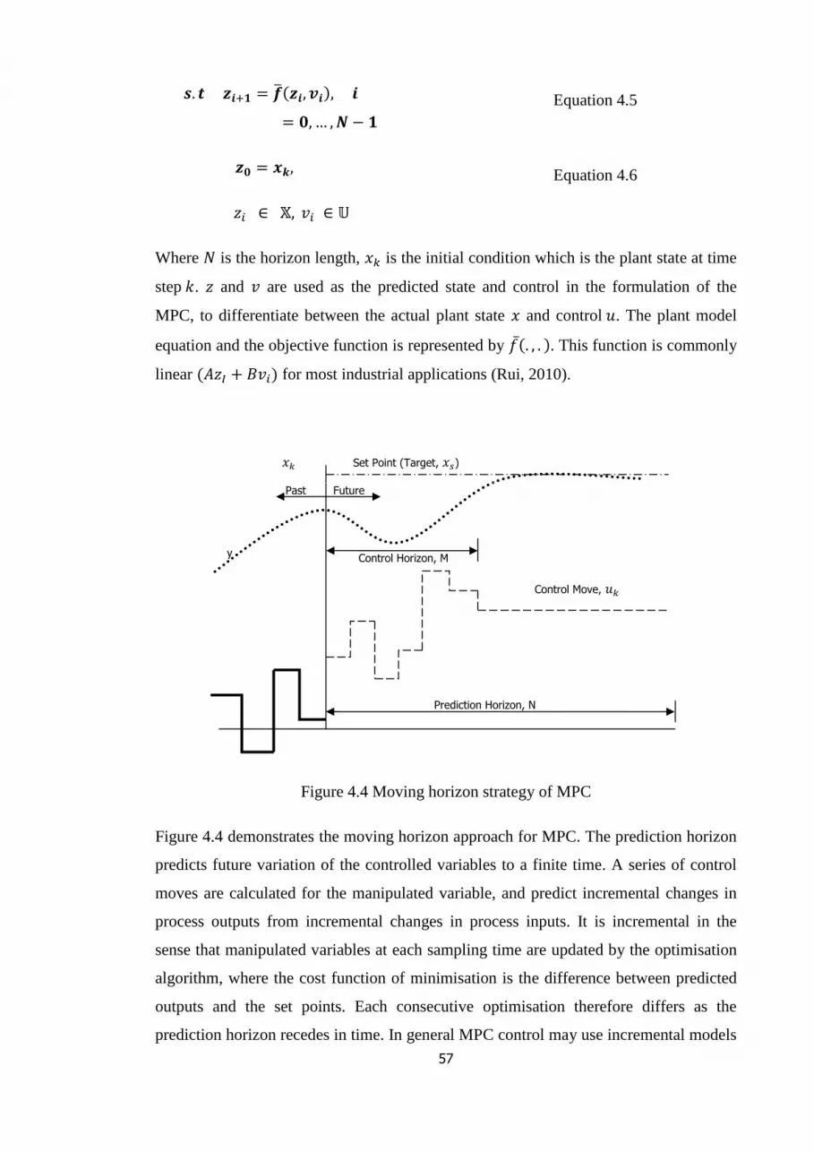
57
𝒔. 𝒕 𝒛𝒊+𝟏 = �̅�(𝒛𝒊, 𝒗𝒊), 𝒊
= 𝟎, … , 𝑵 − 𝟏
Equation 4.5
𝒛𝟎 = 𝒙𝒌,
𝑧𝑖 ∈ 𝕏, 𝑣𝑖 ∈ 𝕌
Equation 4.6
Where 𝑁 is the horizon length, 𝑥𝑘 is the initial condition which is the plant state at time
step 𝑘. 𝑧 and 𝑣 are used as the predicted state and control in the formulation of the
MPC, to differentiate between the actual plant state 𝑥 and control 𝑢. The plant model
equation and the objective function is represented by 𝑓(̅. , . ). This function is commonly
linear (𝐴𝑧𝐼 + 𝐵𝑣𝑖) for most industrial applications (Rui, 2010).
Figure 4.4 Moving horizon strategy of MPC
Figure 4.4 demonstrates the moving horizon approach for MPC. The prediction horizon
predicts future variation of the controlled variables to a finite time. A series of control
moves are calculated for the manipulated variable, and predict incremental changes in
process outputs from incremental changes in process inputs. It is incremental in the
sense that manipulated variables at each sampling time are updated by the optimisation
algorithm, where the cost function of minimisation is the difference between predicted
outputs and the set points. Each consecutive optimisation therefore differs as the
prediction horizon recedes in time. In general MPC control may use incremental models
y
Prediction Horizon, N
Control Move, 𝑢𝑘
Control Horizon, M
Past Future
𝑥𝑘 Set Point (Target, 𝑥𝑠)

58
of FIR and ARX. These models use current and previous values of process cause signals
to predict process effect signals.
There are a series of calculations involved in MPC control execution; this is depicted in
Figure 4.5. Step one requires knowledge of the current state of the process such as the
state of the inputs of disturbance, manipulated and output control variables. The steps
that follow generally aim to ensure the status and direction of the process is moving
towards steady state and dynamic optimisation (Qin and Badgwell, 2003).
Figure 4.5 Series of flow of calculations conducted for MPC control (Qin and Badgwell,
2003)
State estimation aims to estimate the dynamic state of the system. Failure to include this
concept into the MPC may result in the need for further instrumentation to estimate
additional process measurements. Other effects may include (1) for integrating or
unstable processes, the use of ad hoc fixes to remove offsets and (2) limitations on
unmeasured disturbance models. Thus most industrial MPC control calculation design
incorporates some feedback mechanism.
The determination of the controlled process subset requires the controller to determine
which MV’s to be moved and which CVs to be controlled. This will include the
selection of high and low level control outputs.
Ill-conditioning occurs where a small error in the calculation can result in larger errors.
In the case of MPC, small changes in the controller error can lead to large MV moves
(1) Reading MV, DV and CV
values from the process
(2) Output feedback state
estimation
(7) Output MV’s sent to the process
(6) Dynamic optimisation
(5) Optimisation of local steady state
(4) Ill-conditioning removal
(3) Determination of controlled process subset

59
with a high condition number in the process gain. Such situations require examination
of the condition number at each control execution in order to exclude the ill-
conditioning impact.
The majority of industrial MPC controllers execute local steady state optimisation at
each control cycle. This enables the steady state inputs and outputs to be close to their
targets. The controller may use a linear program (LP), QP or both to conduct the
optimisation and this dependent on the provider and or the nature of the problem.
In terms of dynamic optimisation, changes are made to the MVs to drive the process to
the set steady state by the MPC controller without violating constraints. The constraints
can be hard (should never be violated), soft (some violations are allowed) or set point
approximations where there is penalisation on deviations above or below the setpoint
(Qin and Badgwell, 2003).
Common reasons for failures in industrial applications of MPC include; constraints,
unique performance criteria, process nonlinearities, model uncertainties and cultural
reasons with regards to education, people or financial reasons (Qin and Badgwell,
2003). The cultural reasons such as education, the people or financial reasons are very
critical to the success of the controller in the long term. This is because with a good
understanding of the process from the control engineers, a reasonable MPC with little
model uncertainties can be designed and implemented. The controller is then left with
operators, who will manage and make use of the controller dependent on their training
and the level of time available to maintain the controller which may be financially
constrained. As per the simulation activities conducted so far, some of these are
eliminated; however the nonlinearities and model uncertainties present in AD systems
may make it difficult to achieve a successful application of MPC.
4.3.2 Dynamic model structures
FIR and ARX are popular linear model structures. Process models are central to MPC
and FIR is a popular model structure of choice for MPCs, due to the ease of fitting
complex dynamic systems without the selection of a model structure. FIR uses lagged
inputs for capturing the system dynamics of the process and therefore is commonly non-
parsimonious and a large amount of model parameters are needed. These follow a more
complex modelling approach and includes large data sets whereas parsimonious models
like ARX aim for simplicity (Nounou and Nounou, 2007). ARX uses both lagged

60
inputs and outputs to represent the output and offers greater simplicity. Parsimonious
models also offer models with few degrees of freedom, which can avoid over-fitting a
situation where the model works well in a given range but breaks down in predictability
outside that range. The FIR model can be described as:
𝒚(𝒌) = ∑ 𝑩𝒋𝒖(𝒌 − 𝒋)𝑵𝒋=𝟏 + 𝒗(𝒌) Equation 4.7
Where N corresponds to the settling time and 𝑢(𝑘), 𝑦(𝑘) and 𝑣(𝑘) are the process
input, output and noise vectors respectively. 𝐵𝑗 is the matrix of the coefficients to be
identified models of the FIR can only be applied to stable processes (Qin, 1998; Nounou
and Nounou, 2007).
The ARX model structure predicts the process and the future trajectory of the effect
signals using current and past process cause signals. For a multivariable system such as
the AD, ARX can be represented by:
𝒚(𝒌) = ∑ 𝑨𝒊 ∗ 𝒚(𝒌 − 𝒊) + ∑ 𝑩𝒋 ∗ 𝒖(𝒌 − 𝒋)𝒏𝒖𝒋=𝟏
𝒏𝒚
𝒊=𝟏+ 𝒗(𝒌) Equation 4.8
Where 𝑢(𝑘) and 𝑦(𝑘) are the inputs and outputs of the process data vectors. 𝑣(𝑘) is
vector representing the noise and 𝐴𝑖 and 𝐵𝑗represent matrices for the model coefficients
and 𝑛𝑦 and 𝑛𝑢 are the time lags for the inputs and output variables. This method allows
use of steady-state regression techniques for modelling dynamic processes (Qin, 1998;
Su et al., 2009). Modelling in this form has been applied to AD processes (Premier et
al., 1999).
4.3.3 The quadratic programming algorithm
The aim of the quadratic program optimiser is to move the process to a steady state
optimum operating point. The constraint controller key objective is to hold process
variables at specified setpoint values or within their constraint limits subject to the
actuation variable constraint limits (Perceptive Engineering Ltd, 2012).
𝑱 = ∑ 𝒂𝒊𝒊 ∗ 𝑴𝒊 + ∑ 𝒃𝒋𝒋 ∗ 𝑨𝒋 Equation 4.9
Where 𝑀𝑖 represents the process variables, 𝐴𝑖 as the actuation variables and the cost
assigned to the process and actuation variables as 𝑎𝑖 and 𝑏𝑖. The optimum is maximised
subject to process and actuation constraints. The algorithm is available in most
industrial MPC frameworks where the dynamic model associated with the constraint

61
controller is used to generate the steady state model for use in the optimiser directly.
The QP algorithm is used in the inventory simulation study Chapter 6; to optimise the
system and compare an MPC with and without an optimiser.
4.4 Multivariate statistical analysis
Decision making activities in terms of the monitoring and control of AD processes
require chemical measurements that are reliable and that can be used to enhance the
process control understanding. Rapid technological advancements have resulted in large
volumes of data being stored and retrieved easily, enabling an increase in the
application of data based modelling.
The growing use of data based modelling over the past forty years has resulted in the
advancement of mathematical and logic based methods. The success of data based
technologies is however a result of how accurately and successfully a system is defined
and measured. There has been considerable success in multivariate calibration,
multivariate process modelling & monitoring & pattern recognition, calibration &
discriminant analysis as well as structured modelling (Wold and Sjostrom, 1998).
Pioneers such as Svante Wold and Bruce Kowalski combined mathematical modelling,
multivariate statistics and chemical measurements to develop the field of chemometrics.
These achievements were only possible due to the use of established methods such as
principal component analysis (PCA) and partial least squares (PLS).
The basis of identifying a good quality model relies on the quantity and quality of the
data used for the modelling. It has been suggested that the input data must have a
minimum of 5 measured changes that are of the order of 5 times larger than the noise
associated with the input (Boudreau and McMillan, 2007). The historical data generated
for the feasibility studies lacked this quality attribute and therefore a DoE was required
to improve the quality of the data. This can be carried out by conducting step or pseudo
random binary sequence (PRBS) tests. The generation of such data can take months to
years for a system such as the AD.
A further challenge is that some critical parameters such as those affecting the safe
sludge matrix requirement cannot be changed as it will yield non complying product.
These impose constraints and set the boundaries on the process. Thus processes models
such as those for AD are bounded and limited by the degree to which the process can be
excited.

62
4.4.1 Principal component analysis
PCA was developed in 1901 by Pearson (Pearson, 1901) with the geometric
optimisation explanation and later Hotelling’s in 1933 (Hotelling, 1933) reported the
algebraic derivation of PCA. Given a set of data consisting of a large number of
interrelated variables, PCA aims to reduce the dimensionality of the problem whilst
retaining the major sources of variation in the data set (Jolliffe, 2005). For a vector of x
with p random variables, if the variance of p random variables, the structure of the
covariances or the correlations between the p variables are of interest, then for a large
complex p variables, it is best to look for some of the p derived variables that preserve
most of the information given by variances and correlations or covariances (Jolliffe,
2002). PCA concentrates on variances and places less emphasis on covariance and
correlations (Jolliffe, 2002). However although PCA focuses on variance, it does not
ignore correlations and covariance (Jolliffe, 2005).
The inferential sensor study uses PCA to examine the relationships between variables
within the AD process data, since there are a large number of measured quality
variables which are highly correlated. Through the approach of PCA, dimensionality of
the multivariate data is reduced whilst still retaining the original variables as each
principal component is a linear combination of the original variables. This enables the
representation of the original data set containing correlated variables, in a new ordinate
system that is characterised by uncorrelated variables called principal components
(PCs).
𝑿 = 𝑻𝑷𝑻 + 𝑬 Equation 4.10
Where X is the process variables, T is the score matrix, P is the loadings matrix and E is
the errors. X may be decomposed through singular value decomposition (SVD) or
nonlinear iterative partial least squares (NIPALS). The procedure was carried out using
Matlab software with the PLS toolbox (Wise et al., 2010). The data was first autoscaled
before applying PCA since the variables have different units. As PCA aims to capture
variation, autoscaling enables all variables to be treated on an equal basis in the analysis
and therefore variables that have greater variation due to the magnitude of the variable
do not dominate variables with a smaller order of magnitude of variation.
PCA has various assumptions, which include linearity, large variances having important
structure and PCs are orthogonal. There are methods available for modelling nonlinear
63
systems with nonlinear PCA approaches (Martin, 2010). Process knowledge is required
to determine whether PCs with low variance are noise.
PCA is a common and flexible approach used for data compression, information
extraction and preliminary visualisation of samples (Wold et al., 1987; Jolliffe, 2005).
The application of PCA may reduce the dimensionality of the multivariate data into a
smaller number of PCs than original variables. It enables the representation of the
original data set containing correlated variables, in a new reference system that is
characterised by uncorrelated variables of PCs. The PCs are linear combinations of the
original variables calculated hierarchically and are mutually orthogonal. The greatest
amount of variation contained in the original data set is captured by the first PC.
Subsequent PCs captures the next greatest possible amount of variance. Once obtained,
the loadings and scores can be graphically represented to observe any trends or
groupings in the data set, in form of variables and sample respectively.
4.4.2 Partial least squares
Although PCA may be a popular approach in chemometrics for treating sets of data
subject to high dimensionality; it does not offer prediction of a response variable. Partial
least squares or projection to latent structure (PLS) models predict a process output
from linear combinations of a reduced set of independent variables, namely latent
variables. These are typically steady state methods, which eliminate correlations
between inputs (Boudreau and McMillan, 2007). Predictive models can be constructed
for highly collinear systems and involve many factors. PLS is therefore less use for
understanding underlying relationships within a set of data but rather has a general
purpose for response prediction (Tobias, 1995). PLS was pioneered in the econometrics
field by Herman Wold in the late 1960s and later found application in the chemical field
by his son S. Wold and others such as H. Martins and B. Kowalski (Wold, 1966; Wold
et al., 1973; Kowalski et al., 1982; Wold, 2004).
The method of PLS aims to relate two data matrices of X and Y by means of a linear
multivariate model. This method is applied in this research for building predictive
models because of its usefulness in dealing with noisy and collinear data (Ericksson et
al., 2006). As discussed previously MLS has the tendency for over-fitting, where there
may be too many observations. In such cases, there may be a low number of factors
(latent variables) that account for most of the variation in the response. PLS extracts the

64
latent factors which account for most of factor variation and thus avoids the overfitting
issues if the model structure is selected appropriately.
For processes with large a number of factors where collinearity may exist and process
relationships are not well understood such as the AD process, PLS is a useful tool for
constructing predictive models of such systems (Tobias, 1995). Principal component
regression (PCR) aims to find factors that capture the greatest amount of variance in the
predictor (X) variables, whilst multi linear regression (MLR) attempts to find a single
factor which best correlates the predictor and the predicted variables. PLS relates to
both PCR and MLR and attempts to maximise covariance (Wise et al., 2006). Selection
of latent variables (LV) in PLS models is very important as selection of too few or too
many can result in under or over fitting of the model, resulting in a model that fits the
sampled data perfectly but fails to predict new data well. Over fitting violates parsimony
and may lead to poor future performance.
If all the variables in the block are measured in the same units, then no scaling is
required. When the variables in a block are measured in different units, then variance
scaling may be used. This is conducted by dividing all the values in the variable by the
standard deviation of that variable to enable the variance of each variable to be a unity.
Furthermore variables can be given different weights depending on their influence on
the model.
4.4.3 Inferential measurements
Information is used for operating the plants through monitoring and control as well
evaluating the performance of the plant. Predictive models, namely soft sensor, virtual
online analysers or inferential sensor can also be built from this information. Modelling
of these sensors can follow the data driven approach or model driven. Model driven soft
sensors generally are of the form of first principle modelling, which describe the
physical and chemical characteristics of the process. The highly dynamic and complex
characteristic of industrial processes makes use of such model types difficult for
practical use. Data driven soft sensors are therefore more common on industrial
processes and generally use PCA and regression techniques.
The general approach for soft sensor development is depicted in Figure 4.6 A robust
soft sensor must aim to predict with accuracy, precision and reliability but also cope
with measurement noise, data outliers, drifts, missing values and data colinearity

65
(Kadlec, 2009). Inferential measurements improve reliability and reduce process
composition noise but drift and unknowns are inevitable. Data pre-processing
techniques used included visual inspection, removal of bad data, outlier detection and
treatment, data cleaning including filtering and data alignment to reflect process
operation. This process was applied to the simulated and industrial process data selected
for the inferential sensor modelling. Once the simulation and process data was available,
the model development commenced with initial data inspection.
As the offline process data used for the inferential sensor development was measured
infrequently with large variability in when the measurements were conducted, this made
modelling with PLS difficult and therefore less likely to be used in basic process
control.
Figure 4.6 Schematic of inferential sensor development process
4.5 Conclusions
This chapter presented a brief summary of key methods used in this thesis. Multivariate
statistical analysis techniques are used in Chapters 5 and 7 with soft sensor development
in Chapter 7. Multivariate statistical analysis methods are used in this thesis due to the
limitations of increased uncertainty in parameter values and variability imposed by
Initial data inspection
Data selection
Data pre-processing
Model selection and design
Model training and Validation
Soft sensor maintenance

66
models designed with widespread applicability such as ADM1. The virtual plant model
ADM1 has many advantages as described in section 2.3.2.

67
5 Benchmark study
5.1 Introduction
The benchmark study, discussed in this chapter formed the backbone of the feasibility
study. Between the three water companies, four sites were selected (1) Blackburn
wastewater treatment works (WwTW) (2) Mitchell Laithes WwTW (3) Bran Sands
WwTW and (4) Lancaster WwTW. An initial benchmark analysis was undertaken on
the Lancaster mesophilic anaerobic digestion system, but it was later upgraded to the
Monsal Enhanced Enzymic Hydrolysis (EEH) and a further benchmark analysis was
conducted. However due to this change the site excluded from the analysis undertaken
in this chapter but the data from this site is included in Chapter 6, with respect to the
soft sensor development activities. The general findings from the site contribute to the
overall business case and together these four sites provide a good representation of the
various AD technologies available to the water industry.
The aim of the benchmark study is to establish baseline performance using process data
for the existing plants generalised delay steady state behaviour and in the presence of
controlled disturbances. Benchmarking allows the assessment of best practice and the
identification of any bottlenecks inherent to the process as well as providing insight into
the culture with respect to the daily operation of the process. The benchmark study
addresses the following goals:
Comparison of the operational objectives, review current process operational
performance and defining, quantifying, and qualifying the performance metrics;
Investigate the performance of the existing regulatory control system and
identify areas for improvements in terms of advanced control monitoring;
Determine the level of accuracy and precision for current instrumentation and
sampling methods for determining systematic and random errors;
Calculate process capability and performance indices for key process variables.
A crucial part of the benchmarking exercise is focus on monitoring and measurement
systems with respect to control as identified in Chapter 3; this is addressed through the
assessment of (i) process performance (outputs of the process); (ii) the inputs required
to achieve the outputs and (iii) other parameters to ensure that performance is delivered
(Ahmad and Benson, 1999). The robustness of these measurements depends on a
number of factors including the availability of data that provide relevant information,
and the ability to trust the data. Online measurements form the basis of control systems

68
and thus obtaining data from reliable and correctly appropriately operated measurement
systems is crucial. There is a requirement to avoid systematic measurement errors.
Calculating the uncertainties in the instruments allows the controller to be parameterised
and hence operate close to the constraints.
The use of historical process data to benchmark a site enables the determination of the
behaviour of the plant and allows the modelling of its performance through the data
generated from the various processes. There are several challenges with this approach:
The availability of the necessary sensors for monitoring key performance
indicators (KPIs);
Accuracy and validity of the measurement systems for the evaluation of
systematic errors;
Precision and reliability of the measurement systems to account for random
errors.
Without testing the various measurement systems against these challenges, an
assessment of the accuracy and reliability of the data generated cannot be undertaken.
The data used for the analysis is thus assumed be a good representation of the process,
prior to the analysis.
For the identification of relevant KPIs to satisfy the project aims, a hierarchy of KPIs
were identified Figure 5.1. Every organisation will have a set of KPIs to measure their
performance and progression. These may include lost time, employee motivation,
customer written complaints and net energy usage etc. Within the water industry these
may be sewage treatment works breach of consents, water quality, sewer flooding
incidents and pollution incidents. With respect to the AD project, corporate KPIs for the
water companies include a reduction in net energy usage and reduction in CO2
emissions. Electricity consumption generally accounts for over 70 % of the water
companies CO2 emissions and hence reducing the reliance on imported electricity is
important for the companies involved, and this can be achieved through the utilisation
of the biogas produced from the AD process. The energy generated is mainly used on
site with excess exported to the national grid. The objective for the 3 water companies is
then to optimise the AD and combined heat and power (CHP) processes to reduce their
reliance on imported energy. This also satisfies government incentives with respect to
increasing renewable energy resources (ofgem, 2011b). Exported electricity from AD

69
processes is of greater value compared to electricity generated from conventional fossil
derived sources, as per the renewable obligation certificate (ROCs), feed in tariffs
(FITs) and renewable heat incentives (ofgem, 2011a). Maximum energy production and
minimum energy usage thus form the basis of the corporate KPIs. Business unit KPIs
differ between the 3 companies. United Utilities (UU’s) aim is to improve digestate
quality, whilst the exploration of co-digestion opportunities of other waste streams with
sewage sludge is a priority for Northumbrian Water Ltd (NWL). Yorkshire Water’s
(YW) objectives are the overall optimisation of the AD process with CHP operation.
From these business KPIs, various control KPIs are formed and setpoints to be
investigated are generated.
Figure 5.1 The hierarchy of KPI
The benchmark analysis is conducted using Perceptive’s Advanced Process Control
(APC) software systems (Perceptive Engineering Ltd, 2012). Various statistical process
control (SPC) techniques were implemented to analyse the process audit data, process
capability (PC) form the core of the analyses. Pc describes the minimum variability that
occurs when the process is in a state of statistical process control. This is true for
processes where process variability is only due to random and common causes intrinsic
to the process. Combining the capability standard deviation with customer specification,
setpoint or the objective function gives an index which illustrates the best quality
control possible for the process. This enables the identification of any risk in using the
current quality control to achieve the specification.
Process performance indices (Pp and Ppk) and process capability indices (Cp and CpK)
are two metrics that relate specification and variability (Shunta, 1997). These two
Corporate KPIs
Business Unit KPIs
Throughput Yield …….Outages Consent Limits
Production Maintenance Quality Environment
Temperature CH4% OLR VFA pH ………% DS Set Points
Control KPIs

70
metrics together provide information that can be used to guide quality control
improvements through (i) reviewing the current performance of the process, (ii)
estimating any potential improvement in quality and (iii) providing a guide on how
improvements can be achieved. Cp describes the minimum variability occurring while
the process is in a state of statistical process control. This is defined by equation 5.1 as
the difference between the upper and lower specification limits (USL-LSL) divided by
six sigma (6σ). Cp considers only the spread of the data in relation to the specification
limits. This is the state where variability is caused by random or common causes
inherent within the process, thereby giving an index for the best possible control. A high
value of Cp corresponds to a process capable of meeting the specification. Generally,
the rule of thumb is if Cp<1 then the process is unsatisfactory and Cp>1.6 indicates a
process with high capability with Cp between 1 and 1.6 in the medium range of
capability.
𝐶𝑝 = (𝑎𝑙𝑙𝑜𝑤𝑎𝑏𝑙𝑒 𝑟𝑎𝑛𝑔𝑒)
6𝜎=
(𝑈𝑆𝐿 − 𝐿𝑆𝐿)
6𝜎
Equation 5.1
Nevertheless, Pp measures all sources of variability in describing the average operation
by the current control system. Ppk gives an indication of how well the controls maintain
the variability within the desired range. These metrics combined can be used to assess
whether the performance of the process meets its capability. Table 5.1 can be used as a
guide to assess the capability and performance of the process (Shunta, 1997) by
evaluating several KPIs from the process data.
Table 5.1 Process capability analysis
Does performance meet capability?
No (Ppk<<Cp) Yes (Ppk~Cp)
Does capability
meet
specification?
No (Cp<1) Change process
Improve control
Change process
Yes (CP>>1) Improve control Little incentive for
improvement

71
5.2 The benchmark sites
5.2.1 Blackburn WwTW
The Blackburn anaerobic digestion (AD) process was commissioned in 2006 following
an upgrade from a traditional single phase MAD system to the Monsal EEH MAD
technology. The site in Lancashire handles around 13,500 tDS of sludge per year, for
approximately half a million people in the Blackburn and South Lancashire area. Figure
5.2 illustrates a simplified process flow for the advanced digestion process where the
red lines indicate flows of the pre-digested sludge, purple lines indicate the flows of
digestate, green lines indicate flows of biogas, and blue lines indicate heating water
flows. The site utilises its own primary and secondary sludge, plus imported sludge and
cake from other sites, as well food waste. All the feed streams pass into the balancing
tank and are then thickened by the gravity belt thickeners. The impact of the different
waste streams on the digestion process cannot be evaluated as the quantity and quality
of the different streams being mixed are not recorded.
The dataset was extracted from United Utilities’s OSIsoft1 PI (Process Information)
historian which records data from various AD process control systems of the Blackburn
WwTW SCADA system, programmable logic controller (PLC) and the laboratory
information management system (LIMS) as well as from calculated KPIs.
Approximately 396 signals were collected from 14 January 2010 13:00 to 14 July 2010
12:00, totalling 188 days of data used for the benchmark study.
5.2.2 Mitchell Laithes WwTW
The digestion process at Mitchell Laithes WwTW is a traditional MAD. A simplified
diagram of the process is shown in Figure 5.3. The site located in Dewsbury treats
imported sludge from nearby WwTW and the sites own generated sludge. The data set
used for the analysis was extracted from Mitchell Laithes SCADA system with 110
signals collected over a period of 150 days from 29th
October 2010 at 00:00 to 1st June
2011. The level of instrumentation at this site is limited and consequently, the KPIs of
volatile solids destruction, digestate chemistry, gas composition and the level of
foaming within the digester could not be investigated. This made it challenging to
evaluate the performance of the digestion process and hence most of the analysis mainly
identified bottlenecks in instrumentation and inventory.
1 OSIsoft is a software company manufacturing the PI system of real-time data infrastructure solutions
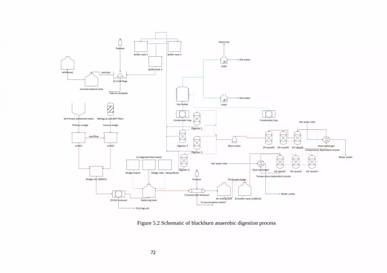
72
16 Primary settlement tanks Biological and BAF filters
Primary sludge Humus sludge
2X Grit removal
Thickened sludge
EH vessel1
EH vessel6 EH vessel4
EH vessel3EH vessel2
Digester 1
Digester 2
Digester 3
Digester 4
Gas holder
Blast cooler
CHP1
CHP2
Condensate trap Condensate trap
2x Centrifuge
centrate balance tank
centratewhitbread
Balancing tankAir mixing tank EH buffer tank (1200m3)
sump2sump1
Sludge silo 1800m3
2 Gravity belt thickener
Sludge import Sludge cake - deliquidised
overflow
Co-digested food waste
Polymer
To accumulation tanks?
Heat exchanger
Temperature dependent recycle
Heat exchanger
Temperature dependent recycleEH vessel5
Polymer
Cake to stockpile
Buffer tank 2Buffer tank 1
Buffer tank 3
Electricity
Hot water
Hot water
Hot water inlet
Water outlet
Hot water inlet
Water outlet
Grit/rags etc
Figure 5.2 Schematic of blackburn anaerobic digestion process

73
Figure 5.3 Schematic of Mitchell Laithes AD process

74
5.2.3 Bran Sands WwTW
The Bran Sands WwTW is one of Northumbrian Water’s regional sludge treatment
centres (RSTC). The 50 acre site was previously partly used for sludge drying. The
company made a strategic decision to invest in a thermal hydrolysis process (THP). Part
of the remit was to utilise as much of the equipment from the old drying plant as
possible which included instrumentation used for the thickening processes. The dryers
are still available on standby should the thermal hydrolysis AD breakdown. The site is
manned 24 hour and treats both domestic and industrial waste. A simplified outline of
the process is given in Figure 5.4.
Figure 5.4 Schematic of Bran Sands AD process
Northumbrian Water identified a number of issues they were working to address prior to
the benchmark study taking place. These included the following:
High operator variation leading to increased variation in the process;
Uncertainty in how to reduce faults and daily breakdown in the operation of the
pumps and belt thickeners;
Uncontrollable high levels of foaming and uncertainty to the causes of foaming;
Variability in terms of quantity and quality of the imported cake potentially
resulting in blockages through an increase in ‘rags’ (accumulation of sticks,
plastics and other materials typically larger than 6mm) in the system and
increased process downtime caused by ‘rags’ in the strain tank;
Adiabatic
Coolers 3x
Digesters 3x
Digested
Sludge Tanks
Digested
RSTC
Phase 2
Biogas Holders
Boilers 2x
Flare Stack
Gas Engines 4x
Key
Biogas storage and upgrading
RSTC phase 1 and 2 and holding areas
2 Stream CAMBI Thermal hydrolysis
ETW
Primary Sludge
Raw Sludge
Storage Tanks
Imported
Liquid Sludge
Tanker
Discharge Tank
Cake
Reception
Sludge Mixing
Tanks
Sludge
Straining
Sludge
Dewatering
Cake
Reception Silo
Blending Pump
Pulper Reactors Reactors Reactors Reactors Flash
Tanks Cambi
Buffer Silo
Pulper Feed
Pump
75
Design limitation of the AD plant. Insulation for boilers and pipes required;
Combined Heat and Power (CHP) units: Performance affected by boiler demand
for biogas supply and heat balance, moisture in the biogas affects performance
significantly and operators need to drain moisture traps continuously to reduce
this affects.
Four operators from the site were tasked with resolving some of these issues and their
findings although excluded from the results of the benchmark study help to build the
business case for the site for sludge inventory control which aided the inventory
simulation study in Chapter 6.
The data set used for the analyses was extracted from the site’s data historian. The site
uses three different systems for monitoring, control and data storage. These are the
XCS5 which is located in the wastewater treatment area, Intouch which was previously
utilised in the old drying plant and which is now used for the belts and dewatering units
for the AD process and finally XCS6 (Oracle) which has been implemented on the
advanced digestion process. 392 signals were extracted during a period of 89 days
between 5th
January 2011 to 5th
April 2011 and these were imported into the
PerceptiveAPC software for analysis. Laboratory data from the operators was also
included with 113 signals between 7th
September 2009 to 24th
April 2011. The data
obtained both from the laboratory and the data historian was subject to significant
amount of missing data, variation in sampling time and hence required pre-processing
prior to analysis.
5.3 Benchmark data analysis methodology
The benchmark analysis was conducted in PerceptiveAPC (Perceptive Engineering Ltd,
2012), Minitab 16 Statistical Software (Microsoft-cooporation, 2006) and Matlab
(Mathsworks, 2012). PerceptiveAPC suite of products consists of real time and off-line
development tools for different industrial sectors and process types (Perceptiveapc.com,
2015) including:
1. PharmaMV for the pharmaceutical sector;
2. WaterMV for the water industry;
3. BatchMV for batch production;
4. ADvisorMV for optimisation of AD systems.
76
PercepticeAPC offers modelling, visualisation and analysis tools which combine
multivariate statistical analysis and model predictive control (Perceptiveapc.com, 2015).
Featuring:
Process analysis: use of univariate and multivariate statistical methods for
detecting outliers, conducting correlation analysis and statistical normality etc.;
Process monitoring: single and multivariable alarm thresholds, fault detection
and diagnoses;
Process modelling: empirical linear and non-linear regression techniques which
include sensitivity analysis and cross validation metrics;
Process control: a range of industrial control algorithms ranging from PID to
model predictive control;
Process optimisation: calculation of optimum solutions for improved control
(Perceptiveapc.com, 2015).
The data from each site was loaded into PerceptiveAPC separately at 5 minutes
sampling interval for the online data which in intervals of seconds. It was decided that
due to the slow dynamics of the Ad system, 5 minute sampling interval was adequate.
Several key steps were followed to pre-process the data to enable analysis on the data as
the process data generated is generally very noisy and contains errors, missing data and
outliers; it therefore required various pre-processing techniques to refine the data. The
systematic pre-processing procedures followed were:
1. Visual inspection;
2. Handling missing data;
3. Outlier detection;
4. Data alignment;
5. Offline data pre-processing to reflect the online data.
The first step for data pre-processing was visual inspection to inspect the full dataset
and identify the signals which required further data pre-processing. The inspection
required use of knowledge of the process so far, the specification ranges for different
parameters and discussion with operators to discuss the data. The visual inspection
revealed long periods of missing data; high ‘spikes’ in the data such retention values
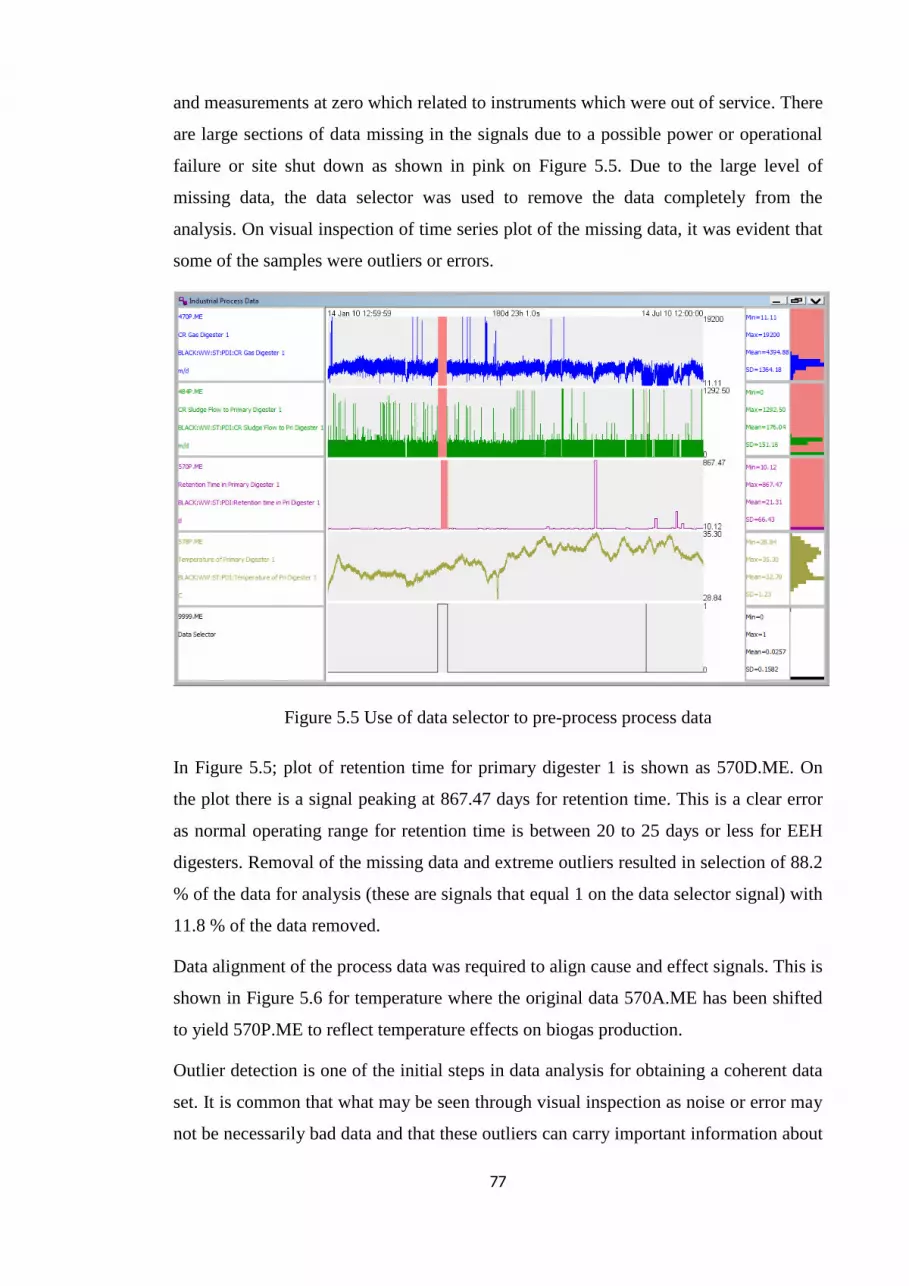
77
and measurements at zero which related to instruments which were out of service. There
are large sections of data missing in the signals due to a possible power or operational
failure or site shut down as shown in pink on Figure 5.5. Due to the large level of
missing data, the data selector was used to remove the data completely from the
analysis. On visual inspection of time series plot of the missing data, it was evident that
some of the samples were outliers or errors.
Figure 5.5 Use of data selector to pre-process process data
In Figure 5.5; plot of retention time for primary digester 1 is shown as 570D.ME. On
the plot there is a signal peaking at 867.47 days for retention time. This is a clear error
as normal operating range for retention time is between 20 to 25 days or less for EEH
digesters. Removal of the missing data and extreme outliers resulted in selection of 88.2
% of the data for analysis (these are signals that equal 1 on the data selector signal) with
11.8 % of the data removed.
Data alignment of the process data was required to align cause and effect signals. This is
shown in Figure 5.6 for temperature where the original data 570A.ME has been shifted
to yield 570P.ME to reflect temperature effects on biogas production.
Outlier detection is one of the initial steps in data analysis for obtaining a coherent data
set. It is common that what may be seen through visual inspection as noise or error may
not be necessarily bad data and that these outliers can carry important information about

78
the process. As such removal of what may be deemed to be as outliers can lead to a
model giving incorrect results, misspecification and biased parameter estimation (Ben-
Gal, 2005). The univariate hampel filter (Hampel, 1971; Hampel, 1974) addresses the
issue outliers have on the robustness of an estimator. The hampel filter approach was
then used to remove further outliers such as the spikes in feed and gas data. Figure 5.6
depicts various signals along with their pre-processed signal.
Figure 5.6 Data pre-processing analysis
The offline samples are collected 2-3 times a week and the last sampled value is held
until the next sample point. This results in process parameters remaining constant until
the next sample is taken hence to enable better modelling with the online process data, a
ramp function was used in PerceptiveAPC. The pre-processed data in Figure 5.6 (red
plot) for volatile solids is ramped to the next sample point and therefore only holds the
peak positions. Figure 5.6 shows examples of the signals from the industrial process:
biogas production (blue), digester feed flowrate (green), retention time (purple) and
digester temperature (dark green). There are missing values (pink) for some of the
online data due to plant shutdowns. Additionally there are spikes in the data and outliers

79
including a large spike in the retention time at 857 days, which is not a feasible value.
The periods covering the missing data and the spikes were excluded from the analysis.
Table 5.2 List of Key Performance Indicators (Horan, 2009)
Parameter Range Units
Biogas yield 0.1-1 m3 kg VS
-1
Energy produced per kg vs-1
Various KW KG VS-1
Energy generated 0-4x10⁴ KW hr
-1
H2S <1000 ppm For some CHP units
H2 and CO2 1-5 % and 0-50 % % in biogas
Methane yield 50-80 % in biogas
0.2-0.8 m3 kg
-1 VSapp
100-286 m3.CH4.VS.CODfed
% gas flared 0-100 Varies
Gas Holder level Process dependent Varies
HRT 14-25 days
Alkalinity 1000-3000 Mg L-1
Temperature 30-40 for MAD systems oC
Polyelectrolyte usage 0-300 Kg day-1
Optimum feed rate 0-500 m3 day
-1
Feed TS (%) 4-8 % % of total volume
VS removal 50-65 % %
VS destruction 30-90 % %
Digestate quality Various means to satisfy PAS 110 Varies

80
Using the process design specification settings and list of typical key performance
indicators in Table 5.2, time series analysis was conducted on the datasets to determine
the internal structure of the data. The results for these are discussed in Section 5.4.
5.4 Benchmark results
5.4.1 Blackburn enhanced enzymic hydrolysis MAD
Time series plots were conducted for each of the samples to investigate the data. Several
key findings were identified and a summary of these key findings are discussed in this
section.
Currently the % DS is controlled manually by the process operators through adjusting
the amount of polymer in the gravity belt thickeners (GBTs), which reduce the sludge
volume through removal of water and thickening of the sludge. For this process the %
DS has a specification range of 5 to 7 %. The process capability chart Figure 5.7,
illustrates the offline % DS for the Blackburn site Figure 5.7a and the online % DS for
Mitchell Laithes Figure 5.7b. The red lines indicate the lower and upper specification
limits and the black distribution curve indicates the normal distribution for the data
whilst the blue curve identifies the theoretical minimum distribution that can be
achieved as per minimum variance control. 40 % of the time, the % DS is outside of
specification for the Blackburn site when the offline measurement is recorded. A
consequence of the sampling periods; samples extracted at 3-5 days intervals; the
variability is of the same order as the standard deviation cannot be reduced due to the
low sampling frequency. By sampling at a higher frequency, random process or
measurement variations in the % DS could be observed and mechanisms put in place to
reduce the level.
On examining the quality metrics of the % DS data from Blackburn, Cp is less than 1
which indicates that there is excessive random variability inherent in the process and
Ppk~Cp confirms that this random variability may be reduced by changes to the process
such as through improved measurement procedures thereby ensuring % DS is closer to
specification. This can be achieved by online % DS analysis as observed for the
Mitchell Laithes site, in Figure 5.7b. Montgomery (2005) defines quality as being
inversely proportional to variability. The reduction of variability in the process and its
outputs enables quality improvement. These are the reasons why a reduction in
variability is important for maintaining consistent quality.

81
Figure 5.7 Process capability chart for online and offline % DS
The sludge feed % DS to the digester usually does not exceed 10-12 % due to
limitations in pumping. High % DS may result in high yields of gas and may give an
indication of the contents of nutrients and organics available for the microorganisms to
feed on depending on the particular waste. A high % DS is shown to correlate with high
yields of biogas (Barber, 2005b). % DS composition is maintained through the addition
a) Blackburn offline
% DS distibution
b) Mitchell Laithes
% DS distribution
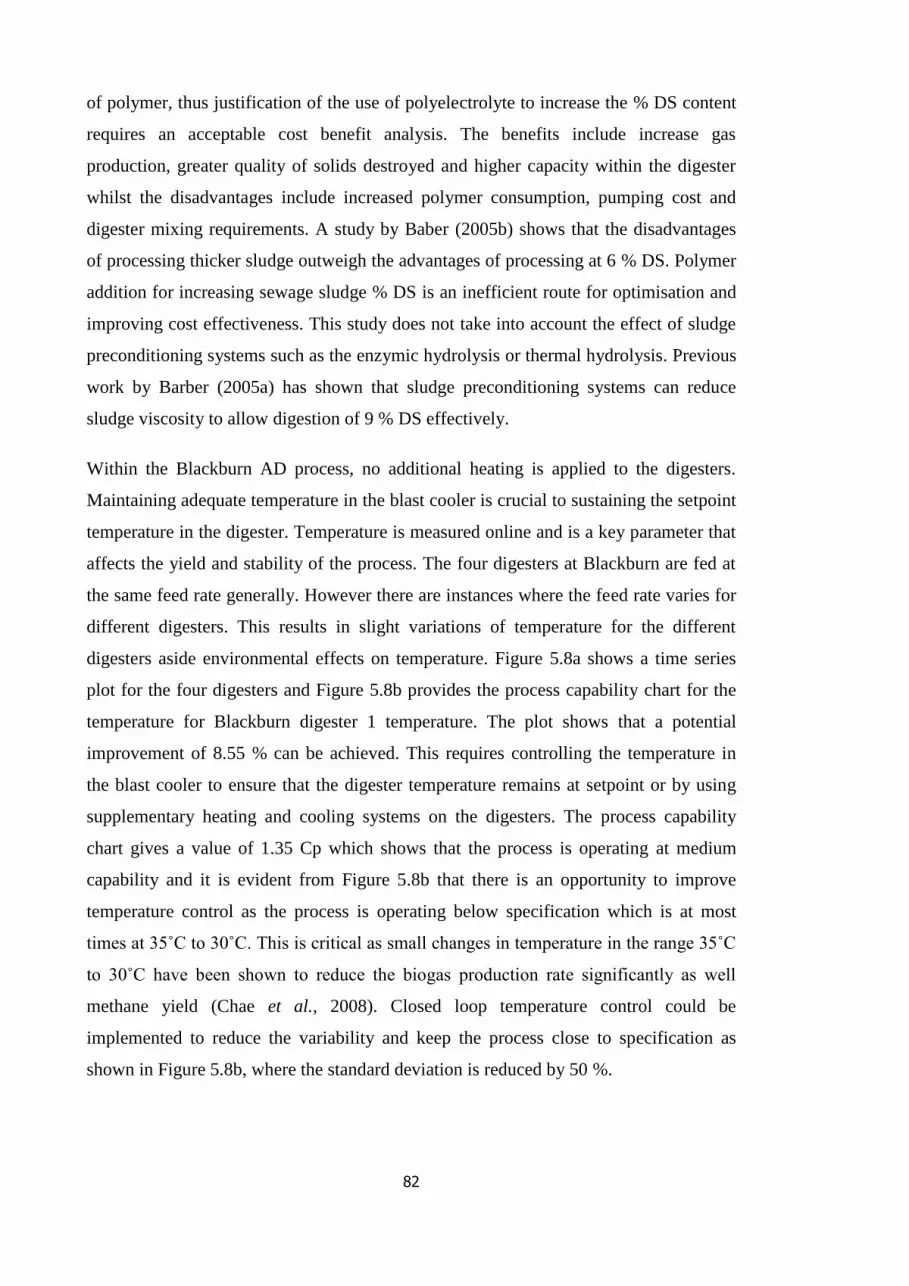
82
of polymer, thus justification of the use of polyelectrolyte to increase the % DS content
requires an acceptable cost benefit analysis. The benefits include increase gas
production, greater quality of solids destroyed and higher capacity within the digester
whilst the disadvantages include increased polymer consumption, pumping cost and
digester mixing requirements. A study by Baber (2005b) shows that the disadvantages
of processing thicker sludge outweigh the advantages of processing at 6 % DS. Polymer
addition for increasing sewage sludge % DS is an inefficient route for optimisation and
improving cost effectiveness. This study does not take into account the effect of sludge
preconditioning systems such as the enzymic hydrolysis or thermal hydrolysis. Previous
work by Barber (2005a) has shown that sludge preconditioning systems can reduce
sludge viscosity to allow digestion of 9 % DS effectively.
Within the Blackburn AD process, no additional heating is applied to the digesters.
Maintaining adequate temperature in the blast cooler is crucial to sustaining the setpoint
temperature in the digester. Temperature is measured online and is a key parameter that
affects the yield and stability of the process. The four digesters at Blackburn are fed at
the same feed rate generally. However there are instances where the feed rate varies for
different digesters. This results in slight variations of temperature for the different
digesters aside environmental effects on temperature. Figure 5.8a shows a time series
plot for the four digesters and Figure 5.8b provides the process capability chart for the
temperature for Blackburn digester 1 temperature. The plot shows that a potential
improvement of 8.55 % can be achieved. This requires controlling the temperature in
the blast cooler to ensure that the digester temperature remains at setpoint or by using
supplementary heating and cooling systems on the digesters. The process capability
chart gives a value of 1.35 Cp which shows that the process is operating at medium
capability and it is evident from Figure 5.8b that there is an opportunity to improve
temperature control as the process is operating below specification which is at most
times at 35˚C to 30˚C. This is critical as small changes in temperature in the range 35˚C
to 30˚C have been shown to reduce the biogas production rate significantly as well
methane yield (Chae et al., 2008). Closed loop temperature control could be
implemented to reduce the variability and keep the process close to specification as
shown in Figure 5.8b, where the standard deviation is reduced by 50 %.

83
Figure 5.8 Temperature distributions for Blackburn WwTW
a) Digester 1 - 4
temperature
distribution
b) Process
capability chart
for digester 1
temperature
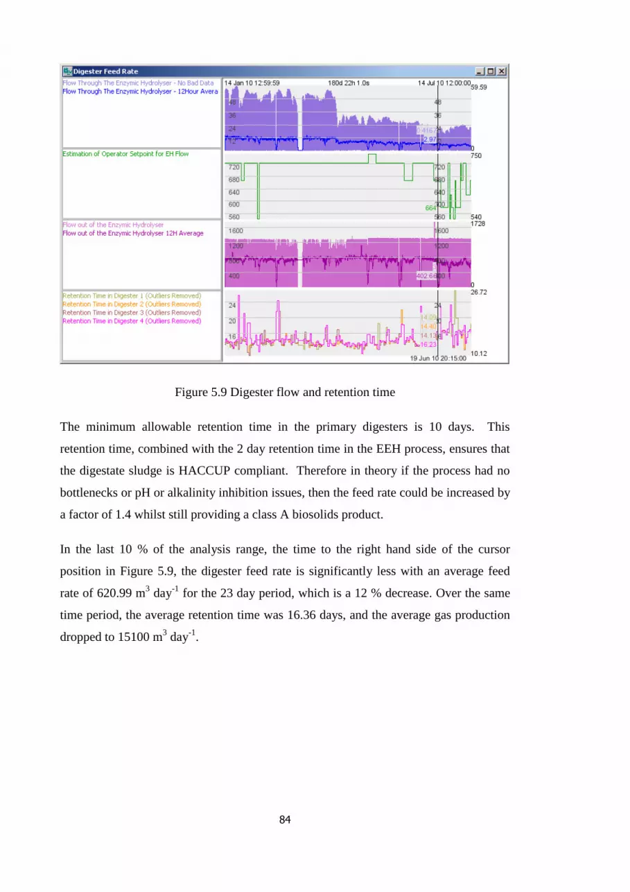
84
Figure 5.9 Digester flow and retention time
The minimum allowable retention time in the primary digesters is 10 days. This
retention time, combined with the 2 day retention time in the EEH process, ensures that
the digestate sludge is HACCUP compliant. Therefore in theory if the process had no
bottlenecks or pH or alkalinity inhibition issues, then the feed rate could be increased by
a factor of 1.4 whilst still providing a class A biosolids product.
In the last 10 % of the analysis range, the time to the right hand side of the cursor
position in Figure 5.9, the digester feed rate is significantly less with an average feed
rate of 620.99 m3 day
-1 for the 23 day period, which is a 12 % decrease. Over the same
time period, the average retention time was 16.36 days, and the average gas production
dropped to 15100 m3 day
-1.

85
Figure 5.10 Gas holder level, volume of gas flared and energy generated
Figure 5.10 shows trend for gas holder level in the uppermost pane, the middle pane
shows the flow to the flare stack, and the lower pane shows the combined electricity
generation of the two CHP engines. It was found that for 1.8 % of the time, the gas
holder level is full and all engines are working to full power and therefore excess gas at
these times require flaring. Therefore the current gas holder and CHPs are unable to
efficiently utilise the gas being generated. There is a need for larger engines, which will
consume more of the biogas. This will reduce the volume in the gas holder and therefore
reduce the instances of gas flaring. CHP2 engine is off when energy generation is below
4000 kWh day-1
and this equates to 19.2 % of the time. If the gas holder level is above
13 meters during this time, then is can be assumed that the outage is due to maintenance
or an unavoidable incident, rather than simply switching the CHP engine off due to a
lack of available biogas. This happens 9.9 % of the time. The remainder of the CHP
downtime 9.3 % of the total time of the analysis range considered can be regarded as
lost opportunity. In other words, 9.3 % of the time the CHP engines are switched off
due to a lack of available biogas, whilst 1.8 % of the time, gas is being flared due to an
excess of biogas. This equates to 8885.51 kWh day
-1 lost on average during these times.
The maximum constant level of energy generation for CHP 2 is about 11300kWh day-1
and therefore the potential to be gained by having the CHP working at these lost times is

86
11300 – 8885.51 which gives 2414.49 kWh d-1
. Assuming that the average cost of
electricity is 6.5p kWh-1
, this gives a monetary estimate of the lost opportunity through
better gas holder inventory management of about £57283.77 per annum. This clearly
shows that the most efficient operation is achieved by maintaining the gas holder level
in the range from 13 m to 13.6 m. If the holder level is in this range, then no gas is
being wasted through flaring, and the CHP engines are running at their maximum rate.
Over the whole analysis range, the gas holder only spends 26.8 % of the time in this
ideal range. Figure 5.11 shows a process capability chart of the gas holder level, with
the ideal range being entered as high and low specification limits. This chart clearly
shows that most of the operating data lies outside of the ideal range and as the flare
stack opens on high gas holder levels, the data is clearly not normally distributed, so the
process capability analysis can only be considered to be a rough approximation. Even if
theoretically 'perfect' minimum variance control were to be achieved, much of the
distribution will still exceed the specification limits, so the complete elimination of
flaring with the current hardware configuration may be impossible.
Figure 5.11 Process capability chart of the gas holder level
The majority of the analyses conducted for the Blackburn WwTW site were univariate
to fully understand the relationship between the different variables as well as
relationships between the observations and variables, principal component analysis
(PCA) was conducted using the PLS toolbox in Matlab (Wise et al., 2010). Based on

87
the data available, and KPIs identified in for the Blackburn AD, a total of 13 variables
were selected for the PCA. Figure 5.12 provide the loadings plot for the first 4 principal
components (PCs). As can be observed, a number of variables are closely related
including foam depth and foam level, i.e. as foam level increases, foam depth will
increase. pH measurements are sensitive to temperature, and thus pH measurements are
temperature dependent.
These analyses allow the confirmation of the theory behind the process and where this is
aligned with practice increases the reliability of the data set. Volatile matter (VM)
appears to be unrelated to the other variables. VM gives an indication of the quality of
the sewage sludge and consequently is expected to correlate with biogas yield. This is
not evident from the results. Providing there is a stable digestion process at constant
retention time, % DS prior digestion and post digestion will also correlate. This may
give an indication of the variability in feed composition. Thus % DS of the digestate
may not necessary be controlled by the % DS of the feed. Volatile matter, volatile acids
and sewage sludge chemistries may perhaps have greater effect on the digestate quality
than % DS.
a) Loadings Plot PC1/PC2 b)Loadings Plot PC3/PC4
Figure 5.12 Loadings plot for PC1-PC4
Investigation of these variables affect the output parameters of biogas yield, post
digestion % DS and foam levels, the data generated from Blackburn was undertaken
through a DoE analysis in Minitab 16 Statistical Software (Microsoft-cooporation,
2006). It was assumed that the variables are linearly related. Table 5.3 shows the
-0.5 -0.4 -0.3 -0.2 -0.1 0 0.1 0.2 0.3 0.4 0.5-0.4
-0.3
-0.2
-0.1
0
0.1
0.2
0.3
0.4
0.5
Loadings on PC 1 (26.76%)
Loadin
gs o
n P
C 2
(16.0
7%
)
Temperature
Pressure
FeedFlow
FoamDepth FoamLevel
RetentionTime Alkalinity
pH
VA
VM
Post%DS
Pre%DS
BiogasY
Variables/Loadings Plot
-0.6 -0.4 -0.2 0 0.2 0.4 0.6 0.8-0.8
-0.6
-0.4
-0.2
0
0.2
0.4
0.6
Loadings on PC 3 (11.38%)
Loadin
gs o
n P
C 4
(9.7
6%
)
Temperature
Pressure
FeedFlow
FoamDepth
FoamLevel
Retention Time
Alkalinity
pH
VA
VM
Post%DS
Pre%DS
Biogas Y
Variables/Loadings Plot

88
estimated effects and coefficients when gas production is the output parameter.
Temperature, feed rate, retention time, feed % DS and their interactions effects on gas
production was analysed.
A standard method of assessing the goodness of fit for a statistical model is the
coefficient of determination R2. R
2 is the quotient of the variances of the fitted values
and observed values of the independent variable, given by:
𝑟2 =∑(�̂�𝑖 − �̅�)2
∑(𝑦𝑖 − �̅�)2
Equation 5.2 (Yau, 2015)
where 𝑦 is the observed values of the independent variable, �̂�𝑖 is the fitted value and �̅�
is the mean. R2 lies between 0 and 1 and if R
2 is equal to 1, the model is a perfect fit to
the data whereas if R2 is 0, the model is unsatisfactory or the mean is the best fit. For
these reasons the R2 values observed are very low for the Blackburn analysis crucial
variables which affect gas production in a digestion process are not included as the data
is unavailable. For example, although the % DS is included, an increase in % DS does
not directly correlate to an increase in gas production as it depends more on the quality
of the sludge. Measurement of feed sludge composition and quality is thus required with
information of sludge age, amount of primary and second sludge, level of biodegradable
substrate, and the types of organic material. Other external factors include mixing,
volatile fatty acid (VFA) accumulation and pH effects which are also not included.
The final results for estimated effects and coefficients for biogas yield are shown in
Table 5.3. These provides that all four factors, temperature, feed flowrate, retention time
and % DS have a significant effect on biogas yield. Although this is well understood
and the reasons are clear, it provides additional credibility to the data generated from the
site in that it captures the linearity theory. The effect of retention time is an interesting
finding as it is monitored to generally ensure compliance.

89
Table 5.3 Final estimated effects and coefficients for gas produced
Term Effect Coef SE Coef T P
Constant -81.4 60.48 -1.35 0.181
Temperature 576.0 288.0 79.58 3.62 0.000
Feed flow 485.6 242.8 79.58 3.92 0.000
Retention time -600.2 -300.1 96.97 -3.09 0.002
Feed % DS 857.6 428.8 117.80 3.64 0.000
Temperature x Feed flow -644.2 -322.1 104.91 -3.07 0.003
Temperature x Retention time 1337.5 668.7 165.28 4.05 0.000
Temperature x Feed % DS -634.6 -317.3 99.45 -3.19 0.002
Feed flow x Retention time 548.1 274.0 106.58 2.57 0.011
Feed flow x Feed % DS -1169.9 -584.9 157.85 -3.71 0.000
Retention time x Feed % DS 1165.0 582.5 115.12 3.76 0.000
Temperature x Feed flow x Retention
time
-1356.7 -678.3 223.73 -3.03 0.003
Temperature x Retention time x Feed %
DS
-959.7 -479.8 124.73 -3.85 0.000
Feed flow x Retention time x Feed % DS -1506.6 -753.3 201.86 -3.73 0.000
S = 41.1282, PRESS = 248518, R2 = 38.70 %, R
2 (pred) = 32.79%, R
2 (adj) = 32.75 %
Figure 5.13 shows four plots demonstrating the effect of various factors on biogas
production. The normal plot Figure 5.13a identifies the factors or combination of factors
which have the greatest effect on biogas production. The plot shows that the
combinations of temperature and retention time have the highest percentage effect on
gas production.
Contour plots are used to explore the potential relationship between three variables. The
two contour plots in Figure 5.13c and 5.13d explore the 3-dimensional relationship in
two dimension of (c) Feed % DS vs gas production and temperature and (d) retention
90
time vs gas production and temperature; where the darker the colour, the higher the feed
% DS and retention time (Microsoft-cooporation, 2006). As such high feed % DS is
given by temperatures below 32°C and gas production rates between 130 and 200 m3 d
-
1. The contour plot in Figure 5.13d for retention time vs gas production and temperature
was more scattered as there are two optimums for retention time as such it is difficult to
draw conclusions from this. However a positive correlation is expected and the results
are inconclusive, as there is a requirement for further validation of this analysis with
new robust data. Economical aims for processes such as AD systems aim to produce
high yields of products at low energy consumption usage as quickly as possible, thus by
improving the efficiency of the process, lower temperature with short retention times
resulting in high levels of biogas produced is the ideal economic benefit. The contour
plots show that this had not been achieved; there is therefore a strong requirement for
monitoring the incoming sludge to better estimate which condition can yield an efficient
optimum gas production.
Figure 5.13 Factor effect analyses
43210-1-2-3-4
99
95
90
80
70
60
50
40
30
20
10
5
1
Standardized Effect
Pe
rce
nt
A Temperature
B FeedF low
C RetentionTime
D FeedDS
Factor Name
Not Significant
Significant
Effect Type
BCD
ACD
ABC
CD
BD
AD
AC
AB
D
C
B
A
Normal Plot of the Standardized Effects(response is GasProd, Alpha = .05)
35.014531.1231
250
200
150
100
199.928
26.717712.8201
250
200
150
100
7.443.95
Temperature
Me
an
FeedFlow
RetentionTime FeedDS
Main Effects Plot for GasProdData Means
Temperature
Ga
sP
rod
35.034.534.033.533.032.532.031.5
225
200
175
150
125
100
75
50
>
–
–
–
–
–
–
< 4.0
4.0 4.5
4.5 5.0
5.0 5.5
5.5 6.0
6.0 6.5
6.5 7.0
7.0
FeedDS
Contour Plot of FeedDS vs GasProd, Temperature
Temperature
Ga
sP
rod
35.034.534.033.533.032.532.031.5
225
200
175
150
125
100
75
50
>
–
–
–
–
< 15.0
15.0 17.5
17.5 20.0
20.0 22.5
22.5 25.0
25.0
RetentionTime
Contour Plot of RetentionTime vs GasProd, Temperature
91
Key findings from Blackburn can be summarised as:
1. Significant level of variability in the % DS;
2. Opportunity for digester temperature control;
3. Low gas yield with performance below design specification;
4. Foam level build-up and effects on biogas production on the whole process;
5. Low volatile solids destruction;
6. Digester feed rate limitation due to inventory;
7. CHP engine capacity limitation;
8. Sludge inventory scheduling, cause of large instability within the process;
9. An optimum identified for gas holder level efficiency range;
10. Opportunities for online instrumentation.
These results can be classified into two groups (i) bottlenecks inherent in the process (1-
5) and (ii) bottlenecks associated with inventory and instrumentation (6-10). Through
discussing with the operators and from the conclusions drawn from the initial findings,
it was clear that before optimisation of the actual process can be achieved, in terms of
optimising biogas production, and stabilising the process, the bottlenecks in inventory
and limitations associated with scheduling and instrumentation capacity need to be
reduced or removed.
It was calculated that by increasing the CHP unit capacity for the site to avoid gas
flaring, about £45,800 per annum could be generated. A further £57,200 per annum
could be generated by aligning the energy production with CHP unit. Furthermore a
considerable amount of money could be generated from scheduling of biogas
production to align with the CHP capacity. This depends on a constant feed rate to
stabilise the digestion process. However operators have little control over imported
sludge with respect to frequency, quantity, quality and limited capacity for storage; the
feed rate is mainly determined by the buffer tank level. Reducing the variability in these
factors could massively reduce the overall variability and instability in the process.
The analyses performed for this site identifies significant bottlenecks which may be
improved with increased in instrumentation and robust monitoring to enable control of
the process. A summary of the key bottlenecks are:
Infrequent feed % DS monitoring;
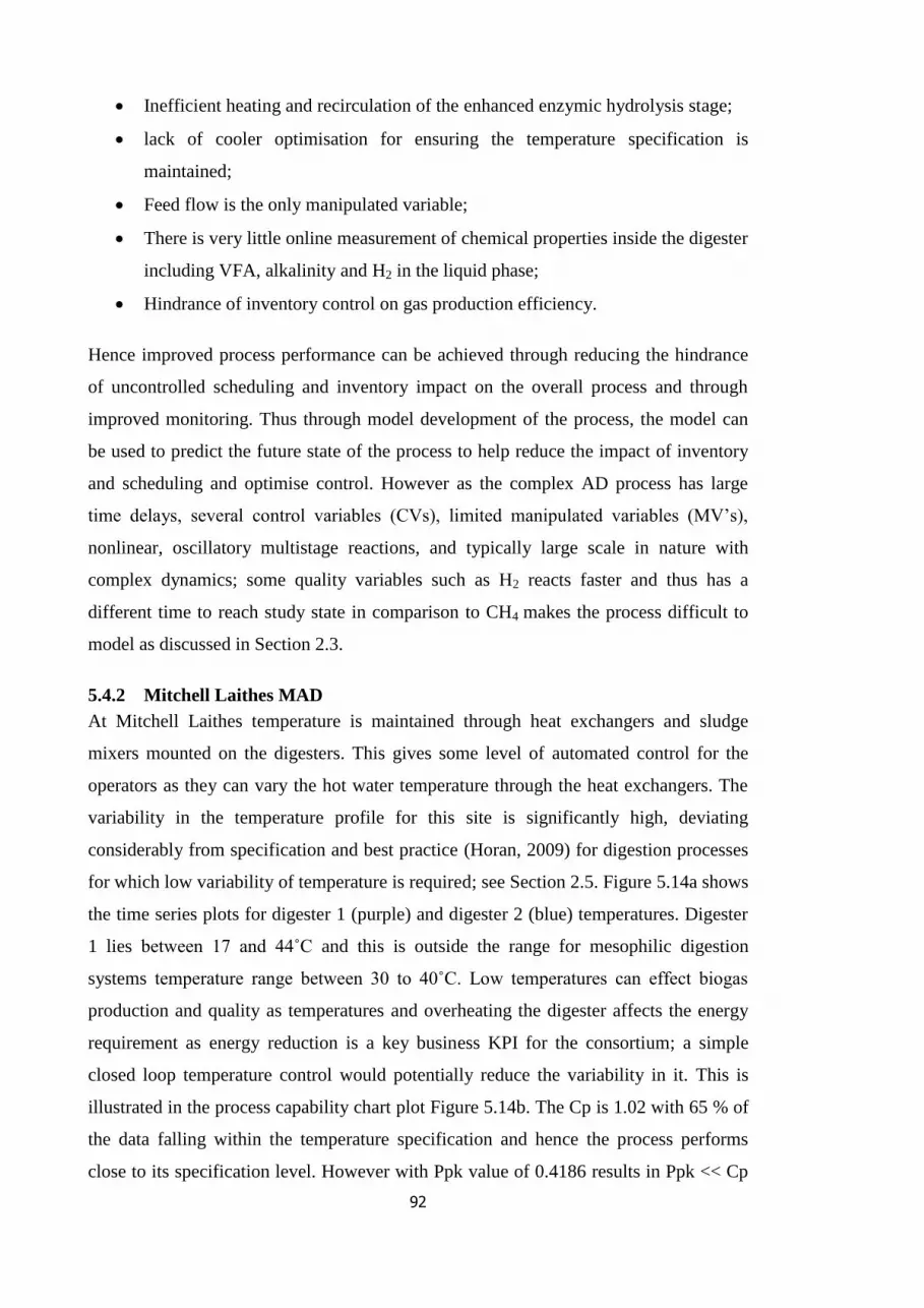
92
Inefficient heating and recirculation of the enhanced enzymic hydrolysis stage;
lack of cooler optimisation for ensuring the temperature specification is
maintained;
Feed flow is the only manipulated variable;
There is very little online measurement of chemical properties inside the digester
including VFA, alkalinity and H2 in the liquid phase;
Hindrance of inventory control on gas production efficiency.
Hence improved process performance can be achieved through reducing the hindrance
of uncontrolled scheduling and inventory impact on the overall process and through
improved monitoring. Thus through model development of the process, the model can
be used to predict the future state of the process to help reduce the impact of inventory
and scheduling and optimise control. However as the complex AD process has large
time delays, several control variables (CVs), limited manipulated variables (MV’s),
nonlinear, oscillatory multistage reactions, and typically large scale in nature with
complex dynamics; some quality variables such as H2 reacts faster and thus has a
different time to reach study state in comparison to CH4 makes the process difficult to
model as discussed in Section 2.3.
5.4.2 Mitchell Laithes MAD
At Mitchell Laithes temperature is maintained through heat exchangers and sludge
mixers mounted on the digesters. This gives some level of automated control for the
operators as they can vary the hot water temperature through the heat exchangers. The
variability in the temperature profile for this site is significantly high, deviating
considerably from specification and best practice (Horan, 2009) for digestion processes
for which low variability of temperature is required; see Section 2.5. Figure 5.14a shows
the time series plots for digester 1 (purple) and digester 2 (blue) temperatures. Digester
1 lies between 17 and 44˚C and this is outside the range for mesophilic digestion
systems temperature range between 30 to 40˚C. Low temperatures can effect biogas
production and quality as temperatures and overheating the digester affects the energy
requirement as energy reduction is a key business KPI for the consortium; a simple
closed loop temperature control would potentially reduce the variability in it. This is
illustrated in the process capability chart plot Figure 5.14b. The Cp is 1.02 with 65 % of
the data falling within the temperature specification and hence the process performs
close to its specification level. However with Ppk value of 0.4186 results in Ppk << Cp
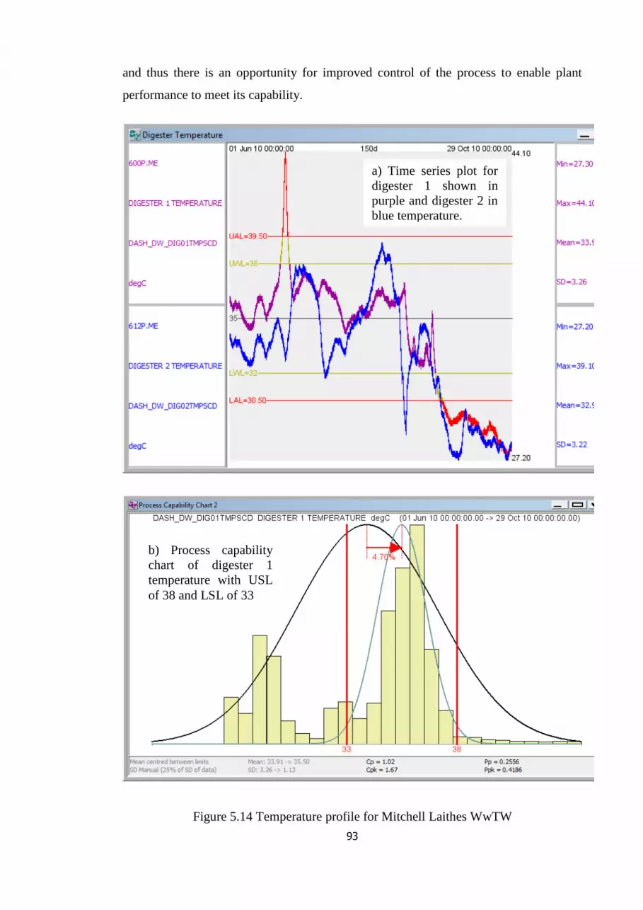
93
and thus there is an opportunity for improved control of the process to enable plant
performance to meet its capability.
Figure 5.14 Temperature profile for Mitchell Laithes WwTW
a) Time series plot for
digester 1 shown in
purple and digester 2 in
blue temperature.
b) Process capability
chart of digester 1
temperature with USL
of 38 and LSL of 33
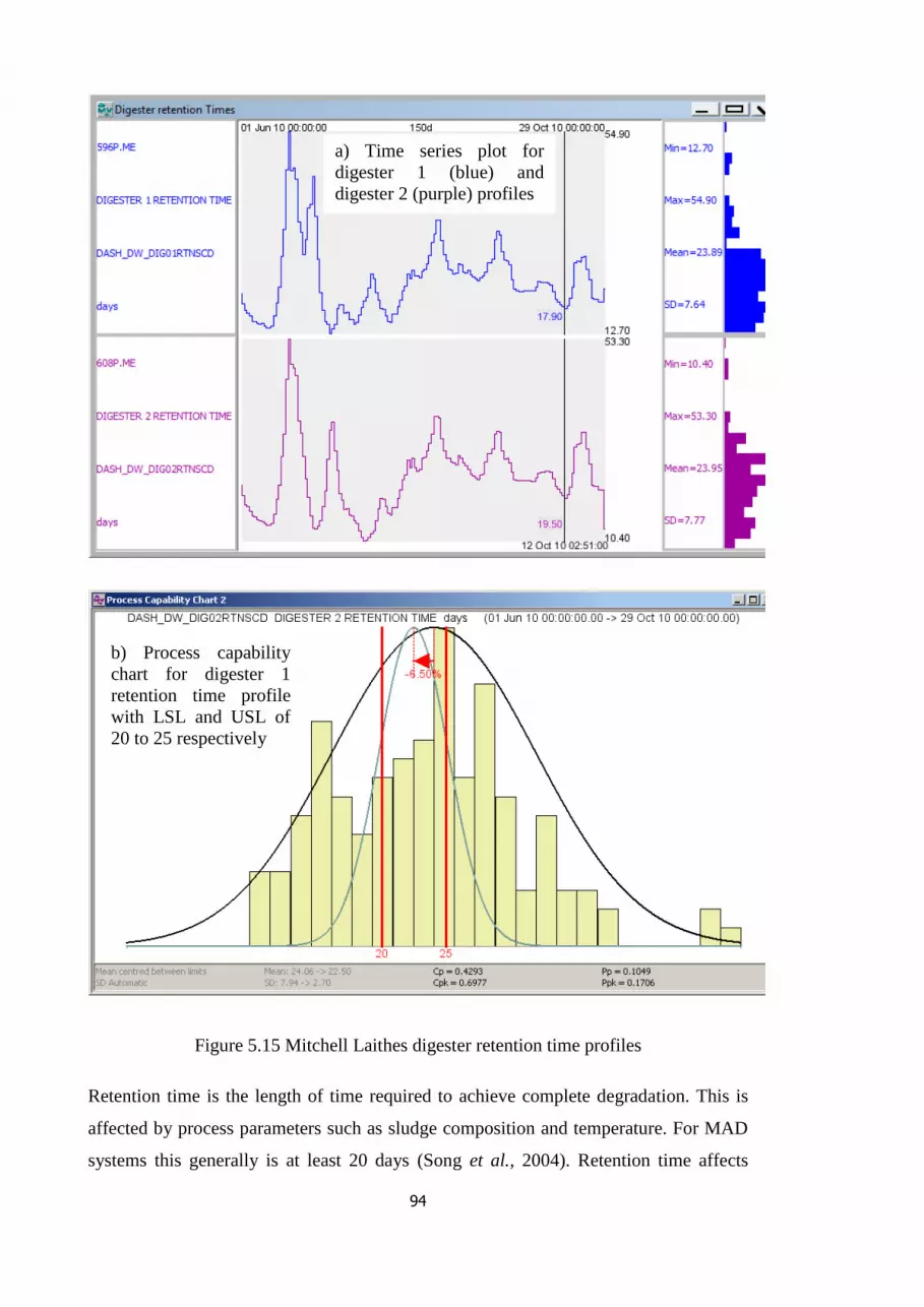
94
Figure 5.15 Mitchell Laithes digester retention time profiles
Retention time is the length of time required to achieve complete degradation. This is
affected by process parameters such as sludge composition and temperature. For MAD
systems this generally is at least 20 days (Song et al., 2004). Retention time affects
a) Time series plot for
digester 1 (blue) and
digester 2 (purple) profiles
b) Process capability
chart for digester 1
retention time profile
with LSL and USL of
20 to 25 respectively

95
digestate quality and therefore compliance. The sludge is expected to remain in the
digester for a minimum time dependent on the temperature of operation and HACCP
ensure that the digestate being spread on agricultural land complies with the relevant
microbiological standards such as the safe sludge matrix (Davis et al., 2010) as HACCP
manage and reduce potential risks to human health and the environment.
Figure 5.15a shows the retention time profiles for the two digesters and Figure 5.15b
gives the distribution of retention time for digester 1. The average retention time for
digesters 1 and 2 were 23.89 and 23.95 days respectively. The minimum allowable
retention time in the primary digesters is 12 days. This retention time, ensures that the
digestate sludge meets the requirements for acceptable digestate quality. However, for
single stage MAD, the optimum digestate quality and biogas production typically
requires over 20 days of retention time. As shown there is significant variability within
the data due to changes in the feed and digestate removal rate, with the retention time
ranging over 42 days. The specification limits for Mitchell Laithes is set between 20 and
25 days shown in Figure 5.15b and digester 1 (blue plot), the process performs within
this specification range for only 27 % of the time. 35.3 % the retention time below 20
days and 37.3 % it is above 25 days offers an opportunity to increase throughput for the
process. Hence for a possible 70 % of the time, the sludge produced does not meet
specification. By reducing the variability in feed flow into the digester, the variability of
retention time may be reduced and the system could be better controlled to
specification. There is scope here for optimisation, by balancing the inventory
management requirements with the aim to minimise the variability in retention time.
Figure 5.16 Primary and imported % DS

96
The Mitchell Laithes AD process had a number of Hach Lange online dry solids
analysers located at various points in the process. Figure 5.16 shows the signal for the
primary imported sludge dry solids and Figure 5.7 showed the process capability chart.
The blue 'theoretical' minimum variance distribution is considerably smaller than the
black 'actual' variance distribution. In other words, it is theoretically possible to control
the % DS much more tightly than it is controlled at the moment. The Figure also shows
that 9.9 % of the data is outside the low specification limit of 4 %, and 32.2 % of the
data is outside the high specification limit of 8 % with an average % DS was 6.83 %.
Figure 5.17 Sludge buffered stock level and digester feedflow
Figure 5.17 trends show the buffered tank stock level and the digester 1 and 2 feedflow
and 12 hour average. Once the buffered stock level drops below approximately 35 %,
both the level signal, and the feed to the digesters tends to stop and over the whole
analysis range, the stock level was below 35 % for 26.8 % of the time, and was above
80 % for 11.8 % of the time. For all of the observed cases when the buffered stock level
was above 80 %, the digester feed rate was running at a reasonably high level.
Therefore for smooth disturbance-free operation of the digester, the buffered stock level
should be maintained above 35 %.
The effect of the feed rate upon the digester temperature is shown in Figure 5.18. In
this figure, before the cursor position, both digester vessels receive almost exactly the
same amount of feed, and the two digester temperatures are correlated accordingly.
After the cursor marker, almost all of the feed is diverted to digester 2, whilst digester 1

97
receives very little feed. This immediately causes the digester 2 temperature to drop,
whilst the digester 1 temperature increases rapidly. When the feed proportion is
swapped later on, the opposite effect happens to the temperature.
Figure 5.18 Digester feedflow effect on digester temperature
The effect of digester feed rate on the gas production is demonstrated in Figure 5.19.
Raw sludge feed rate signals for digester 1 and digester 2 in the uppermost pane of the
plot. Twelve-hour averaged versions of the same signals are shown in the middle pane
of the trend. The bottom trend shows the gas flows from the digesters 1 and 2, and
combined gas flow, and a 12 hour averaged combined flow shown as the black trace.
The averaged gas flow is relatively constant whilst the average feed rate is constant,
however after the first cursor, the feed is shut off for long periods, and consequently the
gas flow drops significantly, ultimately reaching a value of less than half of the original
gas flow before the feed is restored.

98
Figure 5.19 Digester feed flow effect on gas production
Figure 5.20 Site power consumed, generated and exported
The average total site power consumed is 1117.47 kW, whilst the average site generated
power is 505 kW, and the average imported power is 665.85 kW. Figure 5.20 shows

99
plots for the power consumed, generated and imported. The site generated power tends
to be either a high, medium or low value depending on the capacity of the CHP’s. As
the site is almost always importing power, the value of the site generated power can be
calculated based on the import tariff price. This tariff price varies from site to site, and
on a temporal basis. For the purposes of demonstration we have used the following
illustrative figures:
00:00 to 07:00: 4.6 p kWh-1
07:00 to 16:00: 6.7 p kWh-1
16:00 to 19:00: 13.3 p kWh-1
19:00 to 24:00: 6.7 p kWh-1
The average value is £813.82 per day equivalent to £297,000 per annum. This value
does not include the value of renewables obligation certificates. Clearly the value of the
electricity produced is highly temporal, depending on the current tariff, and the number
of CHP's running. Assuming that the biogas storage capacity can be adequately
managed, it is theoretically possible to increase the value of the power generated to
£974.44 per day equivalent to £355,670 per annum simply by aligning the peak tariff
with the peak CHP generation. This represents a value increase of £58,626 per annum,
or a 19.7 % value improvement.
Key findings from the Mitchell Laithes site are:
Significantly high variability in the retention time of the process;
The site produces very little electricity of approximately 0.49 MWh tDS-1
, which
is below what is observed for similar AD systems 0.8-0.9 MWh tDS-1
;
Feedflow limitations imposed by upstream and downstream sludge thickening
and dewatering instrumentations (GBTs, Centrifuges, belt thickeners), which
affects the availability of thickened sludge;
Online % DS data analysis showed significant variability in the data and that the
process was operating outside specification for a large period;
The site compares well with generalised MAD systems, producing 297 Nm3
tDS-1
of biogas which fits into the upper range observed for typical MAD’s of
200-300 Nm3 tDS
-1;

100
There is a significant bottleneck with respect to controlling the temperature close
to specification as there is large variability observed.
General conclusions from this site are similar to those of Blackburn WwTW. The effect
of inventory and scheduling effects on the digestion process were more evident on this
site. The opportunity for a predictive controller to reduce the variability in the feed
through better prediction of inventory is essential. The efficiencies of systems such as
the centrifuges can be greatly improved. There are various sludge thickening devices
available such as centrifuges, belt thickeners, thickening drums and other dewatering
units. Analysis can be conducted to evaluate the efficiencies of these systems to better
inform the water companies on ways to reduce the bottlenecks these instruments impact
on the downstream processes of the overall digestion process.
5.4.3 Bran Sands CAMBI MAD
Measurements of temperature within the digester are obtained from three probes. These
are placed in the upper, middle and lower levels of the digester. Figure 5.21a shows a
plot of the temperature for digester 3, and it can be observed that the average
temperature for all three levels is about 41˚C thus considering the 2500m3 size; digester
there appears to be good temperature distribution throughout. This is achieved by a
closed loop temperature control system. The variability is further greatly reduced in
comparison to Blackburn and Mitchell Laithes; thereby highlighting the potential for
reducing variability in temperature through a closed loop control system.
Water content of the sludge is one of the most important factors with regards to the total
energy demand of the thermal hydrolysis. The hydrolysis temperature plays a key role
in the energy balance. CAMBI recommends 165˚C as the optimised temperature based
on experience. Temperatures for the reactors are not available however temperature of
the sludge coming out of the flashtank is on average 111˚C. CAMBI states that this
temperature (out of the flash tank) should be about 102˚C and ‘practically kept
constant’. Figure 5.21b shows the actual temperatures from the flash tanks which
fluctuate considerably. By deviating from the design on key parameters such as this,
Bran Sands digestion operates below the designed energy balance for the system.

101
Figure 5.21 Temperature profiles for digester 3 and the flash tanks
a) Digester 3
Temperature
Distribution
b) Temperature
out of Flash
Tanks
102
The process design states that 12.3 % DS in the reactor as the optimum. The viscosity at
12.3 % DS is low enough to ensure good homogeneity of the sludge and steam mixture.
Figure 5.22a gives the offline results for % DS for the two pulpers. The energy balance
is based on the sludge feed into the pulper at 15.9 % DS. The injection of recycle steam
from the flash tank and the reactor leads to approximately 14 % DS of sludge out of the
pulpers. There is considerable variation in the pulper output % DS in Figure 10a. The
variation in sludge input to CAMBI is ±1.0 % DS about the hourly average that was set
for the design. The % DS from the digester recirculation units is given in Figure 5.22b.
The range is between 5 and 7 % DS. This is low for a CAMBI process as one of the key
design benefits of the CAMBI technology is that it can handle % DS at a level of 14 %.
Thus the process is performing below its capabilities.
Offline analysis of % DS from the pulpers Offline analysis of % DS from digester
recirculation
Figure 5.22 Analysis of % DS from the pulpers and digester recirculation
For mesophilic digestion, CH4 is generally in the range between 65-68 % of the gas
concentration and 32-35 % for CO2. Figure 5.23a gives the signal for the whole analysis
range and not all of the 94 day analysis range is shown in this trend, additionally, the
CO2 composition measurement only appears to be available from the 24th of February
onwards. Figure 5.14b show trend for both signals in the range where there is data for
both signals from 01 January 2011 to 05 April 2011 with CH4 composition between the
range 58-64 % and CO2 between 44-51 %. CH4 composition is at the low end of the
specification resulting in high CO2 levels in the gas phase. Analysis of the CH4 signal
reveals that the gas component swings through a range of 10 %. Sensitivity analysis

103
conducted using the AD spreadsheet (Redman, 2010) showed that a 1 % increase in
CH4 composition results in an approximately 1.7 % increase in the energy content of the
biogas. For this reason, maintaining high CH4 composition in the gas may have a greater
effect on the energy produced than increasing biogas yield.
Plot of actual CH4 (green) and CO2 (blue)
composition in biogas for the analysis range
Zoomed-in plot of actual CH4 (green)
and CO2 (blue) composition in biogas
for a section of the analysis range
Figure 5.23 CH4 and CO2 composition analysis
CH4 content may be increased through:
Co-digestion: improving the substrate composition improves CH4 content
(Callaghan et al., 1999; Sosnowski et al., 2003; Lehtomäki et al., 2007; Astals et
al., 2011; Zhang et al., 2011). This is however difficult to assess as the different
feed streams need to be investigated to assess the CH4 yield potential;
Temperature: temperatures between 32-35˚C are deemed to be the most efficient
for stable continuous production of CH4 for mesophilic digestion (Song et al.,
2004; Chae et al., 2008; Ward et al., 2008). At low temperatures CH4 content
tends to be higher while biogas yield as a whole is lower;
CH4 production may increase with increasing organic loading rate (OLR) (Ince
et al., 1995) prior to overloading. As there is significant variability in the CH4
content for the Bran Sands data, monitoring and control of parameters such as
the feed rate may be used to control the CH4 composition. A study showed that
OLR affects the CH4 composition (Babaee and Shayegan, 2011) and by

104
modelling the effect of feed rate and CH4 into the potential controller can help
with obtaining highest possible yields for CH4.
A second interesting observation was seen for CH4 composition and digester feed rate.
Figure 5.24 shows a 12 hour filtered signal for the digester feed rate in blue and a 12
hour filtered signal for CH4 composition in the gas phase. The data suggests that as the
feed rate increases, CH4 composition decreases. The opposite effect is observed within
the benchmark simulation model 2 (BSM2) (Alex et al., 2008a), where an increase in
feed rate causes an increase in CH4 yield. It is possible that a different variable is
causing the decrease in CH4 yield. This may be due to the feed sludge stoichiometry
such as sludge age, low % DS and variation in the organic matter which might cause the
methanogens reaction step to shift towards the production of increased CO2 yield
instead of CH4. NWL is keen on exploring co-digestion regimes with wastewater
sludge. Analysis of the digestion system with cause effect analysis on changes to sludge
composition and effects on KPIs such as CH4 yield need to be undertaken. This is more
important for this site as there is considerable evidence that the digestion process is
highly unstable due to foaming issues that affect both upstream and downstream
processes.
Figure 5.24 Digester feed flow versus CH4 composition
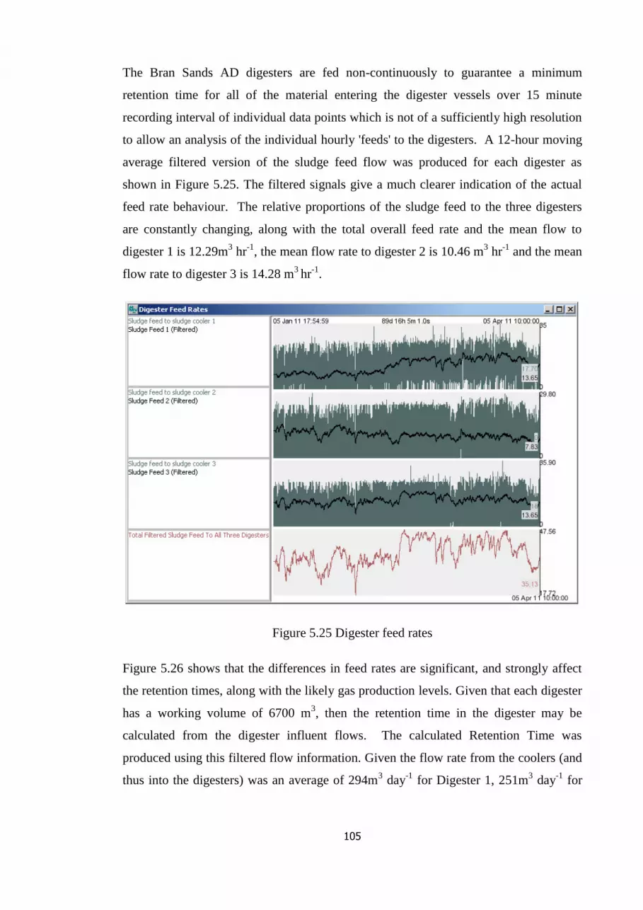
105
The Bran Sands AD digesters are fed non-continuously to guarantee a minimum
retention time for all of the material entering the digester vessels over 15 minute
recording interval of individual data points which is not of a sufficiently high resolution
to allow an analysis of the individual hourly 'feeds' to the digesters. A 12-hour moving
average filtered version of the sludge feed flow was produced for each digester as
shown in Figure 5.25. The filtered signals give a much clearer indication of the actual
feed rate behaviour. The relative proportions of the sludge feed to the three digesters
are constantly changing, along with the total overall feed rate and the mean flow to
digester 1 is 12.29m3 hr
-1, the mean flow rate to digester 2 is 10.46 m
3 hr
-1 and the mean
flow rate to digester 3 is 14.28 m3
hr-1
.
Figure 5.25 Digester feed rates
Figure 5.26 shows that the differences in feed rates are significant, and strongly affect
the retention times, along with the likely gas production levels. Given that each digester
has a working volume of 6700 m3, then the retention time in the digester may be
calculated from the digester influent flows. The calculated Retention Time was
produced using this filtered flow information. Given the flow rate from the coolers (and
thus into the digesters) was an average of 294m3 day
-1 for Digester 1, 251m
3 day
-1 for

106
Digester 2 and 342m3 day
-1 for Digester 3, the retention times in these digesters was
calculated as an average of 25.5, 27.5 and 20.5 days respectively.
Figure 5.26 Digester retention time
Further inspection of the data leads to an interesting relationship between the retention
time in the digesters, and the total energy generated by the gas engines. In this case, the
average digester retention time has a correlation coefficient of -0.8 with the energy
generated from gas indicating a high level of correlation between these variables. This
can be demonstrated visually by comparing the retention time with the inverse of the
energy metric, in Figure 5.27a. This implies that in this instance a reduction in the
average retention time would provide an increase in the energy produced. This can be
further confirmed by inspecting the cumulative sum of the retention time, and of the
energy usage in Figure 5.27b.

107
Figure 5.27 Average digester retention time and cumulative sum – retention time vs
energy produced
At the time of analysis Bran Sands was undergoing several initiatives to address some
of the problems. There are several opportunities which were not revealed from the data
generated. Some of these however need to be resolved to improve the overall efficiency
at the site. The issue of foaming currently means the digestion process is operating
a)
b)
108
below its capability. Further work and analysis is required to remove or reduce this
bottleneck from the process to enable the digestion to reach maximum capability.
The Bran Sands digestion process is fairly new and, as such the level of instrumentation
was expected to be quite high in comparison to sites like Mitchell Laithes. The data
generated from the site did not allow an efficient evaluation of the site’s digestion
process. Key signals such as biogas flowrate and % DS feed to digester were
unavailable making it difficult to compare results from this site with others.
Key findings from Bran Sands are as follows:
Gas flow measurements unavailable;
Inventory and scheduling bottlenecks affecting sludge availability;
CHP engine capacity limitation;
The average energy produced is about 0.34MWh tDS-1
which is well below
typical ranges of 0.8-0.9MWh tDS-1
;
Maintaining efficient heat balance and heat availability;
High % DS variability.
5.4.4 Sensitivity analysis
The data generated from Bran Sands especially had a number of KPI signals missing.
To help with the business case, sensitivity analyses were conducted using the AD
spreadsheet (Redman, 2010). This is a free publicly available spreadsheet, part of a
biogas toolbox designed to assist the AD developer in assessing the viability and
optimisation of different options. There are various feed streams available in the toolbox
however; wastewater sludge characteristics are not modelled as the project is more
aligned with the energy from crops sector.
100 % efficiency is fictional and cannot be achieved as maintenance and repairs are
inevitable. Additional limitations of capital, management ability, labour, communication
and or instrumentation may cause inefficiencies. A 1 % increase in CHP efficiency may
increase income by up to 3 % as indicated by the AD spreadsheet. Various factors may
improve efficiency of the whole site such as optimising feedstock throughput, electricity
and heat production (utilisation of all energy produced through efficient energy balance
for the site), improving the operational efficiency, reducing the feedstock costs and
feedstock capacity could potentially significantly improve efficiency.

109
Figure 5.28 Biogas yield efficiency
Figure 5.28 shows a plot of increasing the efficiency of biogas yield against an increase
in income generated from the process. This is achieved by means of energy production
through CHP units as per the model in the spreadsheet with the value of renewable
obligation certificates (ROCs) (ofgem, 2011b) which doubles the unit value of
electricity. As expected, there is a strong linear correlation between yield increase and
income. The biogas yields from Mitchell Laithes and Blackburn are shown on the plot;
however data for Bran Sands site is unavailable to be indicated on the plot. This analysis
gives a basis for improving the biogas yield efficiency per tDS fed to the digester. A
second analysis was conducted to study the effects of the digester output on the co-
digestion of different waste streams. Wastewater sludge characteristics are not included
in the model and as such are not used in the analysis. As expected there is a positive
increase in value in pig slurry by mixing it with vegetable waste. By knowing the
economics of obtaining certain feedstocks, a cost benefit analysis can be conducted with
the help of analysis such as this to determine the capability of certain co-digestion
regimes.
5.5 Discussions
Due to the level of instrumentation at the three benchmark sites, a comparison between
them is limited. Table 5.4 provides a summary of the KPIs available at all three sites. In
general, there two stage AD processes at Blackburn and Bran Sands outperforms the
single stage MAD at Mitchell Laithes. However, although Bran Sands site is relatively
new the Blackburn site outperforms Bran Sands. This is shown by the level of gas
y = 0.208x - 10.282
-20
0
20
40
60
80
100
120
140
0 100 200 300 400 500 600 700
Inco
me
fro
m C
HP
op
era
tio
n (
£/t
DS)
Biogas Yield (m3/tDS)
Mitchell laithes
Blackburn

110
production per tonne of dry solids fed into the digester, which is more than 4 times the
level gas produced at Mitchell Laithes. This may be due to the quality of the sludge
used at this site, thus without significant analysis of the sludge composition at these
sites, it is difficult to conclude on the reason for the differing performances apart from
the difference in technologies and practices.
Table 5.4 Site comparison of KPI
KPI Blackburn Bran Sands Mitchell
Laithes
Gas produced pet tDS of feed (Nm3 tDS
-1) 453 297 106
Electricity produced per tDS of feed
(MW/tDS)
0.53 0.49 0.209
Organic loading rate (mean in kgVS m3 d
-1) 3.50 1.84 1.68
Digester temperature range (˚C) 27 to 35 38 to 43 27 to 44
Retention number average (days) 14 (+2) 24 23
Digester feed rate (m3 h
-1) 29.34 37.04 19.61
The spread of the data from the three sites varies considerable as shown in Table 5.5.
Although Mitchell Laithes site has a temperature control, the site has the largest
temperature variance.
Table 5.5 Analysis of the spread of temperature data for the benchmark sites
Mean StDev Variance Median Range
Blackburn 31 2.739 7.5 31 8
Bran Sands 40.5 1.871 3.5 40.5 5
Mitchell Laithes 35.5 5.34 28.5 35.5 17
The feasibility study revealed several opportunities in the process; potential savings can
be made by increasing the CHP capacity and aligning energy production with unit
electricity cost price. Long term solutions based around this AD project, include
enhanced monitoring of the process through soft sensor development and the
development of a multi-objective advanced controller to meet the aims of the various
control objectives. The aim of the study was firstly to provide a business case for the
application of an advanced control system to the AD processes.
The benchmark study was carried out with the aim of applying advanced control such as
MPC to improve the process. Significant findings were (1) Inventory and scheduling

111
have an impact on both downstream and upstream processes and form the main
bottleneck in the process; (2) There exist lack of online instrumentations; (3) There is
limited monitoring of the process in general; (4) Offline analyses results in long
sampling intervals; (5) There are quality variables which are not performing at their
specification setpoints and (6) Foaming issues with unknown specific cause.
These formed strong evidence for the project to progress to the development phase to
develop solutions to improve these AD systems. Being an industrially focussed
Engineering Doctorate, the benchmark study is used to evaluate the improvements that
can be gained from using MPC on the AD systems. MPC may be beneficial (i)
continuous process: the availability of feed and the effects of inventory and scheduling
is of high importance. MPC can enable modelling the past feed to allow better
prediction of the future inventory. Controlling the inventory both upstream and
downstream of the digestion process is crucial to optimising the whole process,
advanced control scheme can help with this; (ii) lack of instrumentation: MPC can
harness soft sensor capabilities into the control system and make it possible to reduce
the need for new instrumentations for measurement. However although these form a
strong case for implementation of advanced control system, these cannot be quantified
at this stage due to a lack of relevant data for direct cause effect analysis to establish a
definitive business case. (iii) MPC offers advantage of repeated online optimisation
(feedback) and solving multivariable and constrained with varying objectives and limits
of varying uniformity.
Results generated so far successfully demonstrate an opportunity for advanced control
structures such as MPC and the SWOT analysis in Table 5.6 demonstrates this. The
strengths of the benchmark study lies within the commonalities of the results and the
identification of quick fix money saving solutions. There is opportunity to improve
inventory and scheduling impacts on the AD process thus phase II activities start with
Chapter 6 the inventory simulation which aims to reduce inventory and scheduling
bottlenecks. There is also opportunity to improve monitoring on the process and
Chapter 7 volatile solids soft sensor development aims to achieve this. Weaknesses
identified in the benchmark study results have the potential risks of (i) the necessary
minimum and ideal instrumentation may prove to be unreliable or inadequate to provide
reliable information; (ii) current AD systems may prove to be uncontrollable, large
disturbances or too few adjustable parameters. Difficulty in meeting all or most of the

112
control objectives may increase the complexity of the operation and (iii) real time
experimental testing needed to obtain a rich dataset for modelling may be difficult to
undertake.
5.6 Conclusions
The benchmark study was successful in highlighting significant opportunities for
control and optimisation, implementation of a multi-objective robust advanced
controller that satisfies the aims of the project will be challenging. This is due to the
high level of uncertainty and unknowns within the system. A lack of robust online or
offline instrumentation results in unknown feed composition, uncertainty in the state of
the degradation process and quality of the system outputs. As a result, modelling of the
process has proven to be difficult. Additional studies are required to investigate feed
composition for the various sites, determine potential causes of foaming and digester
degradation pathways to better predict the process outputs.
It can be concluded that no single technology outperforms the other and there are
several commonalities in the performance of the different systems. Increased
monitoring of key parameters and studies into whole plant optimisation such as focus on
the energy balance is essential to improving the performance of the plants.
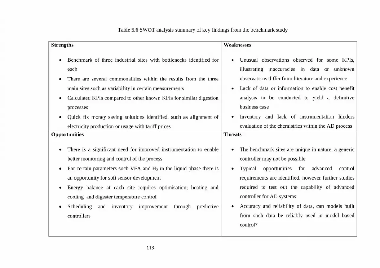
113
Table 5.6 SWOT analysis summary of key findings from the benchmark study
Strengths
Benchmark of three industrial sites with bottlenecks identified for
each
There are several commonalities within the results from the three
main sites such as variability in certain measurements
Calculated KPIs compared to other known KPIs for similar digestion
processes
Quick fix money saving solutions identified, such as alignment of
electricity production or usage with tariff prices
Weaknesses
Unusual observations observed for some KPIs,
illustrating inaccuracies in data or unknown
observations differ from literature and experience
Lack of data or information to enable cost benefit
analysis to be conducted to yield a definitive
business case
Inventory and lack of instrumentation hinders
evaluation of the chemistries within the AD process
Opportunities
There is a significant need for improved instrumentation to enable
better monitoring and control of the process
For certain parameters such VFA and H2 in the liquid phase there is
an opportunity for soft sensor development
Energy balance at each site requires optimisation; heating and
cooling and digester temperature control
Scheduling and inventory improvement through predictive
controllers
Threats
The benchmark sites are unique in nature, a generic
controller may not be possible
Typical opportunities for advanced control
requirements are identified, however further studies
required to test out the capability of advanced
controller for AD systems
Accuracy and reliability of data, can models built
from such data be reliably used in model based
control?

114

115
6 Inventory simulation
6.1 Introduction
The benchmark study in Chapter 4 identified a number of issues including:
1. Inventory and scheduling have an impact on both downstream and upstream
operations and form the main bottleneck in optimising AD processes;
2. There is a significant lack of online instrumentation;
3. There is limited monitoring of the process in general, resulting in a lack of
detailed understanding of the process.
The key bottleneck for optimising industrial AD processes is thus related to the sludge
scheduling and inventory levels. AD processes are typically downstream processes at
wastewater treatment works (WwTW), and therefore the availability of sludge depends
on the upstream processes including activated sludge processes (ASPs), aeration and
settling tanks. Most AD process sites also import sludge from other WwTW sites and
the deliveries are irregular and unpredictable in volume and quality. This was the case
for all the benchmark sites and the operators try to reduce the uncertainty in the
imported sludge volume, quality and frequency to improve the stability of the AD
process. The inventory at any particular site varies considerably and is further impacted
by amounts of storage and or buffer tank availability.
Close control of feed is essential for the stability of the process. This is because feed
flow rate to the digester which is generally the only manipulated variable is dependent
on the level of scheduling and inventory. Constant feed flow is desirable for the stability
of the process as large changes in feed affects the process drastically. More specifically,
large changes in inventory levels results in large fluctuations in feed rate causing
instability in the process. Inventory and feed rate variations act as the main disturbance
in the system. It is therefore desirable to feed the digester with as constant a feed as
possible.
This issue was explored further by designing a simulation to evaluate the capability of a
model predictive controller to control the inventory levels and reduce their disturbance
on downstream processes. It is hypothesised that by removing this disturbance, the true
capability of implementing an advanced controller for the optimisation of the overall
AD system can be identified. A simulation model reflecting the characteristics of the
industrial process and the effect of inventory on its operation was designed. A study was

116
then conducted to test the capability of model predictive control to regulate inventory
levels and to remove or reduce the effect of inventory on process performance.
6.2 The simulation model
The design and details of the simulation can be found in standard Perceptive functional
design specification document titled “Anaerobic Digester Inventory Simulation” giving
a detailed overview of the simulation model. The codes are written in the basic
programming language within the Perceptive Engineering Ltd (PEL) software solution
and this is provided in the disc attached. Perceptive Engineering Ltd has proprietary
rights to the simulation model, therefore only a summary of the model is given here.
The schematic of the simulation process in Figure 6.1 provides the human machine
interface (HMI) using DAQfactory provided by AzeoTech (AzeoTech, 2012). Figure
6.1 provides a schematic of the simulation process. The simulation model begins with
the Gravity Belt Thickener (GBT) where an unknown composition of sludge is
thickened. Thickened sludge from the GBT flows into the thickened sludge silo or
buffer tank. Sludge flowrate and percentage dry solids (% DS) are the two variables
available to the GBT. Dynamic data from Blackburn WwTW is streamed into the GBT.
The rate of the streamed data is scaled depending on the time of the week. The streamed
flow is multiplied by 1.2 for weekdays and 0.5 for weekends. This is because on
observing the inventory levels of sludge at benchmarked sites; inventory levels at the
beginning of the week were very high and at weekends there were no deliveries apart
from Bran Sands WwTW for which there are considerably low deliveries on weekends.
Therefore, the inventory available on these sites reduces considerably on weekends.
This is crucial knowledge to add into the simulation as it enables an opportunity for
maintaining constant feed to the digester and depicting the important disturbances into
the system.
The simulation also contains a heating circuit as depicted in Figure 6.2. Waste heat
energy from the CHP is used to heat a hot water circuit with additional heat provided by
a backup boiler. Heat is lost from the system either from the main digester vessel
through convection, conduction, or from adiabatic coolers. The thermal inertia of the
adiabatic cooler is simulated as a first order response with time delay and the setpoint
value for the adiabatic coolers is negative, to denote heat flow out of the system; whilst
the thermal inertia of the backup boiler is simulated as a first order response with time

117
delay and the setpoint value for the backup boiler is positive, to denote heat flow into
the system. The adiabatic coolers and backup boilers are controllable elements in the
simulation. This enables an analysis for optimising the energy production and the
overall heat balance for the system to address one of the project aims of the overall
project for reducing carbon footprint. Cost elements for heating and cooling the system
are implemented into the model to enable best operation to be maintained.

118
Figure 6.1 Schematic of AD inventory simulation

119
Figure 6.2 AD simulator heating circuit

120
Figure 6.3 Programming signals specification page
121
6.2.1 Simulator structure model
The model consists of seven auto regressive with exogenous inputs (ARX) model
blocks which form the basis of the simulation. These block models relate to:
1. Thickened sludge tank;
2. Heating water temperature after combined heat and power (CHP);
3. Digestate tank;
4. Heating water temperature after coolers;
5. AD gas production;
6. Heating water temperature after backup boilers and;
7. Gas holder level simulation.
The underlying structures of the blocks are recursive least squares (RLS) models. The
block models describe the tank levels, gas production, heating and energy usage in the
system. The simulator enables models identified within the PerceptiveAPC design
system to simulate the AD plant behaviour. The models can be read or fed into the
online system to generate simulated data after model development in the design system.
In configuring a simulator block several properties are required to be specified. These
are:
1. Group level – determines whether the simulator is active or not during online.
Default group signal for simulators is 999.GR operations;
2. Level – determines the conditions under which the block can become active, the
level of the group signal must be higher than or equal to this level;
3. Update interval – defines the interval of the simulator;
4. Sample interval – interval at which new data samples are read into the simulator
algorithm, setting the sample interval smaller than the update interval helps
reduce noise.
For a nonlinear system such as the AD process, linear modelling techniques may be
ineffective at characterising the cause-effect relationships. However, as the simulator
model is simplified to account mainly for heat balance and level control, these factors
are easily modelled and therefore linear models are adequate for this system. The use of
linear model approach is driven by the use of PerceptiveAPC system. Model extensions
of physiochemical and biochemical characteristics of the sludge may require nonlinear
modelling techniques such as neural networks which are available in the
PerceptiveAPC.

122
6.2.2 Simulator design
For the understanding of the behaviour of the AD system over time, it is important to
understand the time response of the system to be able to predict the systems response
and hence, how the ability to implement process control. By understanding the system
dynamics, it is possible to determine the speed of response, the level of overshoot before
settling, oscillations in the system, process instabilities and how rapidly a step change in
a process parameter takes to reach steady state and the rate of change of output
parameters. For an AD process, the dynamics differ for each stage of the digestion
process and also for parameters within a particular process. Therefore understanding the
dynamics at each of the digestion stages and how these affect process parameters is
essential for control.
Current data generated from the benchmark sites fails to provide a complete profile of
the system dynamics of the AD process, with respect to the effect of inventory on the
process. The benchmark data and process understanding resulted in the development of
a simulation model for the optimisation of the inventory. The complex characteristic of
the AD system results in limitations in the developed models of the process and,
consequently, there are inconsistencies between the process model and industrial AD
systems. These issues are due to a lack of in depth process knowledge such as:
Limited number of process interactions being modelled – these are summarised
in Figure 6.3 and focus on parameters that directly or indirectly effect inventory
of the system;
Assumptions on the scale of some unmeasured parameters;
Assumptions on the rate of change of some process effects – the scaling factors
for temperature and feed flow effect on biogas production in Tables 6.1 to 6.3
are assumptions based on theoretical understanding;
Models which do not take into account full indirect effects – for example the
biogas production is based upon a univariate simulation model using the dry
solids signal to the digester as the cause signal for the model with 16 days as
time taken to reach steady state and scale factors for temperature and feed flow
rate applied as summarised in Table 6.1, 6.2 and 6.3 showing temperature
correction, feed rate standard deviation correction and digester temperature
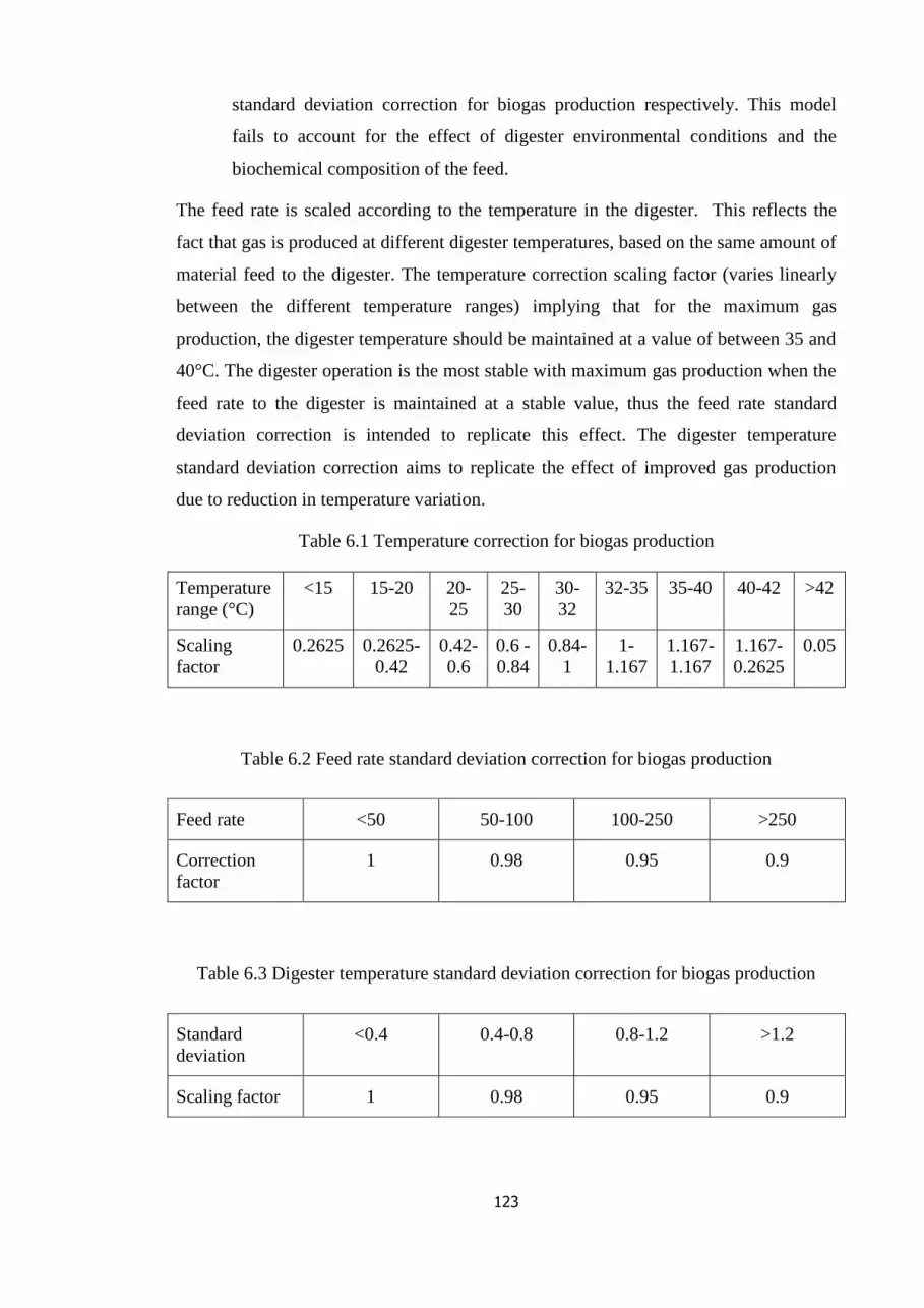
123
standard deviation correction for biogas production respectively. This model
fails to account for the effect of digester environmental conditions and the
biochemical composition of the feed.
The feed rate is scaled according to the temperature in the digester. This reflects the
fact that gas is produced at different digester temperatures, based on the same amount of
material feed to the digester. The temperature correction scaling factor (varies linearly
between the different temperature ranges) implying that for the maximum gas
production, the digester temperature should be maintained at a value of between 35 and
40°C. The digester operation is the most stable with maximum gas production when the
feed rate to the digester is maintained at a stable value, thus the feed rate standard
deviation correction is intended to replicate this effect. The digester temperature
standard deviation correction aims to replicate the effect of improved gas production
due to reduction in temperature variation.
Table 6.1 Temperature correction for biogas production
Temperature
range (°C)
<15 15-20 20-
25
25-
30
30-
32
32-35 35-40 40-42 >42
Scaling
factor
0.2625 0.2625-
0.42
0.42-
0.6
0.6 -
0.84
0.84-
1
1-
1.167
1.167-
1.167
1.167-
0.2625
0.05
Table 6.2 Feed rate standard deviation correction for biogas production
Feed rate <50 50-100 100-250 >250
Correction
factor
1 0.98 0.95 0.9
Table 6.3 Digester temperature standard deviation correction for biogas production
Standard
deviation
<0.4 0.4-0.8 0.8-1.2 >1.2
Scaling factor 1 0.98 0.95 0.9

124
The simulation model was validated and verified to compare the model and its
behaviour to the benchmark sites. This included an iterative calibration process to make
adjustments to the revised model. The objective of the model was to reduce the
disturbances in the process as a result of variation in sludge inventory levels through the
application of a model predictive advanced controller. The hypothesis was therefore; the
model predictive controller can effectively control the sludge inventory levels, thus
improving the stability of the process and maximising biogas and energy production.
This will be illustrated through a reduction in the level of tank level ‘trips’ (i.e. the tank
level violating the upper and lower limits of tank alarm settings), increasing the energy
production and overall site efficiency. The aim of using the simulation in this manner is
to gain further understanding from the process and to utilise this during the plant testing
or design of experiments on the industrial site. Changes made on the plant will thus be a
combination of the results from the simulation results and improved process
understanding. This dynamic model provides a platform for testing control and
optimisation strategies primarily for assessing the capability of a model predictive
control (MPC) controller for removing or reducing the scheduling and inventory
bottleneck.
The benchmark data showed that the industrial systems are subject to several level trips
from the buffer tanks, gas holders, buffer tanks, digestate tanks and centrifuges. Level
trips are incorporated on the buffer tank, thickened sludge silo, digester, digestate silo
and gas holder tanks to trip. This is typical of digestion plant operation and there is a
cost element associated with overflowing the tanks or starting and restarting instrument.
Flow to the buffer tank stops above 99 % full, until the level drops to 90 % full and if
the buffer tank level falls below 1 % full, feed to the digester is tripped to stop until the
level reaches 10 % full.

125
Table 6.4 Simulation level trip signals
Signal ID Description Values
100.ME GBT trip on high thickened sludge tank 0=ok 1=tripped
102.ME AD feed flow trip on low thickened sludge tank 0=ok 1=tripped
104.ME AD feed flow trip on high digestate tank 0=ok 1=tripped
106.ME Centrifuge trip on low digestate tank 0=ok 1=tripped
108.ME Flare on high gas holder level 0=ok 1=tripped
110.ME Trip CHP on low gas holder level 0=ok 1=tripped
112.ME AD feed flow trip on hi-hi gas holder level 0=ok 1=tripped
Table 6.4 and Figure 6.4 provide the level trips occurring for the simulation prior to
controller implementation. As can be seen the level trips occur on a frequent basis and
the thickened sludge tank level overshadows all other trips. The model objective is
therefore to ascertain a way to reduce trips occurring. A base line analysis was initially
conducted from the simulation to establish input or output, data availability, model
structure, parameter estimation and evaluation of model accuracy.
Figure 6.4 Level trips

126
6.2.3 System understanding
Figure 6.5 Step tests for feed flowrate and % DS and their effect on biogas production
Following the completion of the simulator design, step changes were performed on the
manipulated inputs including feed flowrate and % dry solids to observe the changes in
measured outputs such as biogas production. These process excitations or step tests
were conducted to generate data which captured the dynamics necessary for the
modelling. An example of this is shown in Figure 6.5, with step changes of feed flow
rate in blue, % dry solids in green and the result of the step changes shown in the gas
production plot in purple. As can be seen, the peaks and troughs of the gas produced
plot coincide with the step changes of the feed flow rate and % dry solids. The data
generated from the step tests were used to establish relationships within the system and
comparisons were made to ensure the simulation results fitted with what had been
observed or expected to at the industrial sites. This evaluation of system performance
led to an iterative method where the model was continuously updated to make it reflect
more closely to the performance of the industrial process. Some significant findings
from initial simulated outputs were:
The main bottleneck in the process was identified to be the thickened sludge
tank level. The feed to the thickened sludge tank is depicted in Figure 6.6 in blue
over a period of four weeks of simulation time shown in the black division lines.
The figure shows considerable variation over the 4 week period as a direct result

127
of variation in imported sludge. The tank level has the highest number of level
trips and this is shown in Figure 6.4. Knowledge of the scheduling of imported
sludge from other AD is crucial to the control and optimisation of the process;
The simulation also revealed insight into the best initial set points for the system
which limits the amounts of level trips. For example the feed to thickened sludge
tank peaks at about 2393 m3day
-1 with an average or mean flow of about 620m
3
day-1
. These flowrates mean that the tank can fill and empty quite quickly. Feed
flow-rate to the digester can therefore be set to the average flow of the thickened
sludge tank feed to 620 m3 day
-1;
The digestate feed rate to digestate tank level is dependent on digester feed. The
feed flow to digester drastically reduces the digestate tank level; this operates in
an on or off batch mode process (at zero or 2200 m3 day
-1). Knowledge of the
AD feed rate, digestate flow or digestate tank level is required to manipulate the
centrifuge in order not to trip the digestate tank level as this had a great impact
on the tank level.
Figure 6.6 Feed to Thickened sludge tank
The MPC controller enables disturbance profile modelling of expected sludge levels
over the week and therefore a degree of the disturbance can be predicted. Although the
profile varies greatly there is a general drop in the feed to the thickened sludge tank
level over the weekend, this increases generally from Monday, and by Wednesday

128
inventory levels are in the high range through to Friday. Figure 6.6 shows the various
profiles over four days. Modelling of the disturbance profile into the system will help
with reducing disturbances in the system as a whole as the sludge inventory level had a
knock on effect for almost every process in the system.
6.3 Modelling
The PerceptiveAPC model development software uses data driven algorithms to
develop empirical models instead of using first principle models which require
theoretical knowledge of the systems components. The full AD process is too complex
for first principle modelling, for the purposes described here, and therefore the use of
statistical process models to describe the system is followed. Step tests were conducted
to generate an appropriate dataset for the modelling. The training data needed to satisfy
various features to include richness, variability and consistency. This ensured that the
process moves around throughout the data range; the data included all the operating
ranges of the process; to avoid the controller struggling if the process moves to a
different region and the dataset is together in sequence. The MPC models are used to
test the capability of an advanced controller for controlling the process as a whole,
specifically to address the findings from the benchmark study. Two main models were
developed:
1. MPC1: a ‘basic’ structure as the standard MPC control structure depicted in
Figure 6.7;
2. MPC2: a ‘split dynamic’ model structure depicted in Figure 6.8 where the
system dynamics are split into slow and fast characteristics with the aim of
improving total control of the system.
MPC1 in Figure 6.7 shows cause signals on the left hand side in brown (measured
signals), light and dark blue colours as the actuators with effect signals on the right in
light and dark green consisting of set points, state targets and output parameters. The
cause signals are linked to their effect signals by the black arrows. For example, the
measured signal 491.ME feed rate is linked to the actuator signal 1000.AC AD feed rate
which is linked to the effect signals of 332Q.ME Thickened sludge Tank Level (SC),
1000.CT Feed Rate Steady State Target, 478P.ME Biogas Produced By AD (set point),
569P.ME Digestate Tank Level (SC) and 585P.ME Primary Digester Temperature (Set
point).

129
MPC1 and MPC2 both use the same cause and effect signals. MPC2 aims to investigate
the potential improvement for MPC control through separation of the different levels of
system dynamic. Fast dynamic parameters are for example biogas flow, heating and
cooling aspect of the process and slow dynamics are typical parameters contributing to
the production of biogas.
Following the selection of model cause and effect signals, the next step was to set the
model objectives. The main model objective is to avoid tripping the various levels. The
hierarchy of the objectives is summarised in Table 6.5. The lists 9 control objectives and
constraints in order of importance, with 10 being the most important and 2 the least
important. Brief description of the reasons for the objectives and the order of ranking
are also provided in the table. For example, prevention of AD feed stream tripping as a
result of high gas holder level is given the highest level of importance of 10. This is
caused by low levels of sludge in the buffer tank. Avoidance of this is the main aim of
the simulation and ensures constant feed to the system.

130
Figure 6.7 MPC1 basic model structure
288Q.ME Thickened sludge
to buffer tank
1000.AC AD Feed Rate
491P.ME Feed Rate
681L.ME Centrifuge
Run Time (min day-1
)
1010.AC Centrifuge Feed
Rate
480P.ME Gas to CHP
1020.AC Speed / Gas to
CHP
478P.ME Biogas Produced
by AD
1030.AC Biogas Produced by AD Setpoint
585P.ME Primary Digester
Temperature
1040.AC Primary Digester
Temperature
776Q.ME Heat Removed From Adiabatic
Cooling 1050.AC Split Range Adiabatic Cooler / Backup
Boiler 777Q.ME Heat Added Through Backup Boiler 766P.ME Sludge
Dry Solids To Digester
588Q.ME Flow to Gas Flare
750P.ME Ambient
Temperature
697P.ME H-Water Temperature
After Adiabatic Coolers (SC)
695P.ME H-Water Temperature After Backup Boiler (SC)
332Q.ME Thickened sludge Tank Level (SC)
1000.CT Feed Rate Steady State Target
478P.ME Biogas Produced By AD
(setpoint)
569P.ME Digestate Tank
Level (SC)
1030.CT Digestate Tank Level Steady State Target
544Q.ME Gas Holder Level (Setpoint)
585P.ME Primary Digester
Temperature (Setpoint)
696P.ME H-Water Temperature
After CHP (SC)

131
Figure 6.8 MPC2 split dynamic model structure
288Q.ME Thickened sludge
to buffer tank
1000.AC AD Feed Rate
491P.ME Feed Rate
681L.ME Centrifuge
Run Time (min day-1
)
1010.AC Centrifuge Feed
Rate
480P.ME Gas to CHP
1020.AC Speed / Gas to
CHP
478P.ME Biogas Produced
by AD
1030.AC Biogas Produced by AD Setpoint
585P.ME Primary Digester
Temperature
1040.AC Primary Digester
Temperature
766P.ME Sludge Dry Solids To
Digester
588Q.ME Flow to Gas Flare
750P.ME Ambient
Temperature
1050.AC Split Range Adiabatic Cooler / Backup
Boiler
776Q.ME Heat Removed From Adiabatic
Cooling
777Q.ME Heat Added Through Backup Boiler
697P.ME H-Water Temperature
After Adiabatic Coolers (SC)
695P.ME H-Water Temperature After Backup Boiler (SC)
332Q.ME Thickened sludge Tank Level (SC)
1000.CT Feed Rate Steady State Target
478P.ME Biogas Produced By AD
(setpoint)
569P.ME Digestate Tank
Level (SC)
1030.CT Digestate Tank Level Steady State Target
544Q.ME Gas Holder Level (Setpoint)
585P.ME Primary Digester
Temperature (Setpoint)
696P.ME H-Water Temperature
After CHP (SC)
695P.ME H-Water Temperature After Backup Boiler (SC)
1060.AC H-Water Temperature After
Backup Boilers
1020.CT Split Range Heat
Addition Steady State Target
(zero)

132
Table 6.5 Hierarchy of control objectives and constraints
Control objective or constraints Hierarchy
of
importance
Reason
Prevention of AD feed tripping as a
result of high gas holder level
10 Causes feed rate instability. Results in flaring of gas and hence affect CHP
efficiency and energy production per tDS processed
Prevention of AD feed tripping On
high digestate tank level
9 Cause feed rate instability. Increase retention time in the system and hence reduces
throughput in the system
Prevention of AD feed flow tripping
on low thickened sludge tank level
8 Affects all downstream processes. Cause feed rate instability, limits gas production
and results in waste of resources
Prevention of CHP unit tripping on
low gas holder level
7 Affects energy production. Scheduling to improve revenue generation through
aligning energy produced with triad periods
Prevention of GBT instrument
tripping due to high thickened sludge
tank level
6 Affects the upstream processes
Prevention of gas flaring due to high
gas holder level
5 Waste and environmental issue. Currently regulations permit flaring of gas into the
atmosphere. This may change over time with tougher regulations and therefore
there is a greater need to prevent this
Reduction of AD feed rate variability 4 This causes instability in the digestion process and may cause foaming
Increasing the average value of CHP
energy savings
3 Through alignment of energy production with peak electricity selling price
Prevention of centrifuge instrument
tripping on low digestate tank level
2 This affects downstream processes (post digestion)

133
6.3.1 MPC model building in PerceptiveAPC
The modelling page in PerceptiveAPC consists of tabs for specification, coefficients and
evaluation. The specification tab is where the MPC model attributes or details are
specified and this is depicted in Figure 6.9. The coefficients page allows evaluation of
model coefficients followed by model evaluation. The steps followed on the modelling
page are selection of the model details:
1. Model cause and effect signals: the model details begin with the selection of the
model cause and effect signals. These are selected as per Figure 6.7 and 6.8;
2. Block mode: MPC was selected for the block model as a controller model was
required instead of an estimator or simulator model;
3. Model type: Within the PerceptiveAPC framework both linear and nonlinear model
types can be derived.
4. Model structure: the model structure selection enables the user to select absolute or
incremental model structure. The basic finite impulse response (FIR) model format
is modified to enable the history of incremental changes in the cause signals to be
used rather than history of the absolute changes. If a model is nonlinear then the
model is also absolute and incremental nonlinear models are not permitted. As a
linear model type was constructed, the incremental model is selected to improve the
robustness of the model in the presence of unmeasured process drift.
5. Model format: There are three options available in PerceptiveAPC including
principal component analysis (PCA), partial least squares (PLS) and recursive least
squares (RLS). As the linear incremental model type was selected, RLS is the most
appropriate computation algorithm as it enables different paths in the model to be
identified separately using different sets of data, as all coefficients in the model are
changed when the model is identified in PCA and PLS models (Jiang and Zhang,
2004; Perceptive Engineering Ltd, 2012). Therefore, linear RLS models allow ‘path
by path’ modelling, which is achieved by masking out other paths, which is required
as per Figure 6.7 and 6.8. Modelling each path separately allows different
coefficients to be selected and the effectiveness of each path on the overall model
can be identified.
Figure 6.10 illustrates example of four variables affecting temperature prediction.
The diagram shows the fastest approach of making changes to temperature is
through the changes to the feed rate (A). The cold sludge coming into the digester
cools the digester down faster than changes in ambient temperature, cooler or boiler

134
settings and gas flow to the CHP units. Within the simulation, the incoming sludge
is of lower temperature, which means the heating of the digester is more difficult or
happens slower than the cooling of the digester when cooler sludge is continuously
fed into the digester.
The next fastest effect on the digester temperature is the cooler or boiler settings
(D), where there is an initial delay to bring the temperature to the set point. This is
followed by a faster response, provided that the disturbances are kept to a minimum.
Ambient temperature (B) affects is the third effective cause signal, but unlike the
other factors, this is an environmental disturbance which cannot be controlled. The
CHP speed (C) had the lowest effect. Understanding of the model coefficients
enables further understanding on how to control the overall process;
6. Model response structure: The choice of multiple or single effect structure model
depends on the type of model required. For multiple effect structures, the effect on
the prediction of any effect signal involves all other effect signals from the
multivariate structure. This allows effect signals to be cross-coupled in the resulting
structure. Single effect eliminates the cross-coupling, which is ideal for model based
controllers as it can reduce poor effects (through bad data) in the effect signals and,
therefore, making the model more robust.
7. Order of dynamics and Delays: The order of dynamics specifies how many of the
previous samples of the effect signal are used in conjunction with the cause terms to
predict the effect signals trajectory. A higher order of dynamics may provide better
prediction during unmeasured disturbances and may also yield a model less
sensitive to process noise. In this case the order of dynamics was set to one to enable
ARX modelling type. For control applications, an order of dynamics of 1-3 is
typical. The number of auto regressive nodes is determined by the order of dynamics
assigned to the model; for FIR models, the order of dynamics is set to zero and the
difference between the min and max delay should be longer than the longest
transient time to steady-state of any of the effect signals.

135
Figure 6.9 PerceptiveAPC V4.1 modelling page
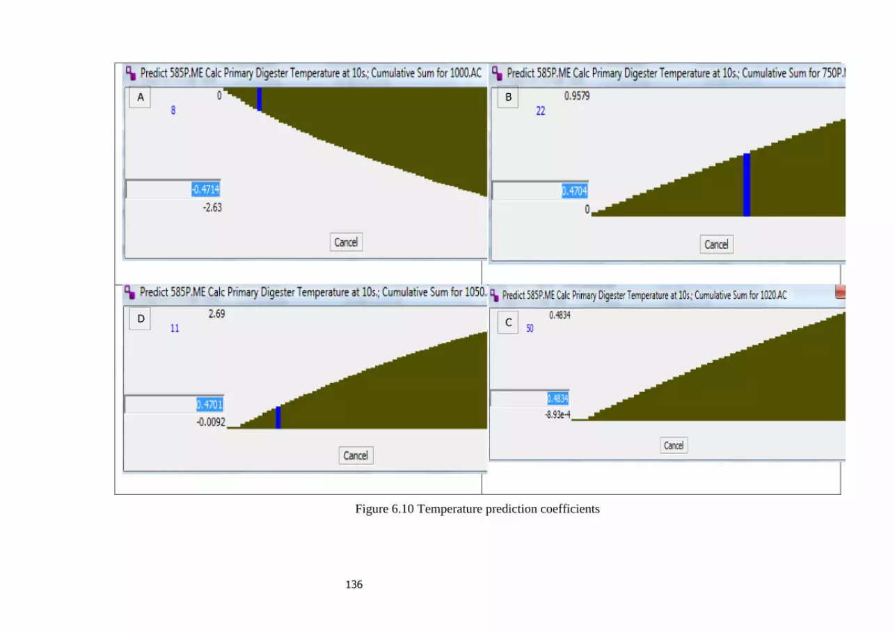
136
Figure 6.10 Temperature prediction coefficients
A B
D C

137
6.3.2 PID model
A PID controller was designed in PerceptiveAPC using basic code. The code is included
in the disc attached. The PID model was designed to control temperature by
manipulating the feed rate. Detail analysis of the model has not been conducted due to
software licence expiration of the PerceptiveAPC, however the PID model was
evaluated at 33°C setpoint and the results is compared with MPC1, MPC2, split
dynamic model and the optimiser model.
6.4 Controller testing
Following the development of the MPC controller in Section 6.3, the next step was to
evaluate the controller performance through a series of scenario evaluation tests. There
were:
Evaluating the MPC1 controller structure in Figure 6.7, this forms the standard
controller for the inventory simulation;
Evaluation of the MPC2 ‘dynamic’ two level structure in Figure 6.8 to test the
impact of splitting the system dynamics into 2 models of fast and slow dynamics
on controller performance;
Alternative controller comparison with a conventional controller such a PID. A
PID controller is developed and simulated to compare results with MPC1 and
MPC2 and evaluate the performance between traditional and advance
controllers;
In addition, an optimiser was developed to test and evaluate the performance of
MPC1, MPC2 and the PID controller scenarios with an optimiser to test for
controller performance with the optimiser.
These four evaluation scenarios helped to assess the need for an advanced controller,
and were compared to the design benchmark system where there is ‘no control’. This
forms the general status of the benchmarked sites in Chapter 5.
6.4.1 MPC1: the benchmark structure system evaluation
The benchmark structure MPC1 was evaluated to understand the capabilities of MPC.
MPC1 model was loaded into PharmaMV Real-Time environment as depicted in Figure
6.11. The Real-Time environment allows models developed in the development
environment to be deployed in real time. The figure shows the specification page for the

138
response signals (the top section of the figure) and cause or predictor signals at the
bottom of the figure.
The Real-Time environment has a controller monitor management framework where the
model specification can be set. The specification for MPC1 can be set to include the
order of priority, hard and soft constraints, and high or low set point settings for the
different signals. A series of overnight runs of the simulation was conducted to
iteratively change the settings to tune the controller to yield optimum performance.
Five examples are provided in this section which includes obtaining the optimum
setpoint for feed rate, adiabatic cooler, back-up boiler setting, digestate tank level, CHP
feed rate and ambient temperature effect on digester temperature.

139
Figure 6.11 PharmaMV 4.1 Controller Monitor management screen
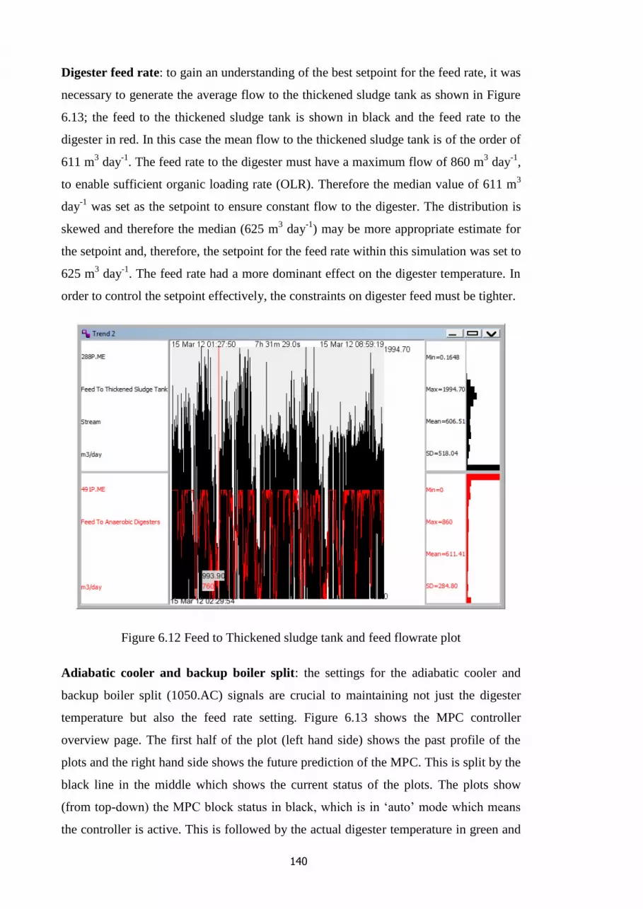
140
Digester feed rate: to gain an understanding of the best setpoint for the feed rate, it was
necessary to generate the average flow to the thickened sludge tank as shown in Figure
6.13; the feed to the thickened sludge tank is shown in black and the feed rate to the
digester in red. In this case the mean flow to the thickened sludge tank is of the order of
611 m3 day
-1. The feed rate to the digester must have a maximum flow of 860 m
3 day
-1,
to enable sufficient organic loading rate (OLR). Therefore the median value of 611 m3
day-1
was set as the setpoint to ensure constant flow to the digester. The distribution is
skewed and therefore the median (625 m3 day
-1) may be more appropriate estimate for
the setpoint and, therefore, the setpoint for the feed rate within this simulation was set to
625 m3 day
-1. The feed rate had a more dominant effect on the digester temperature. In
order to control the setpoint effectively, the constraints on digester feed must be tighter.
Figure 6.12 Feed to Thickened sludge tank and feed flowrate plot
Adiabatic cooler and backup boiler split: the settings for the adiabatic cooler and
backup boiler split (1050.AC) signals are crucial to maintaining not just the digester
temperature but also the feed rate setting. Figure 6.13 shows the MPC controller
overview page. The first half of the plot (left hand side) shows the past profile of the
plots and the right hand side shows the future prediction of the MPC. This is split by the
black line in the middle which shows the current status of the plots. The plots show
(from top-down) the MPC block status in black, which is in ‘auto’ mode which means
the controller is active. This is followed by the actual digester temperature in green and

141
the MPC prediction of digester temperature in brown. The 1050.AC is shown in blue,
with its target setpoint in pink with the red lines showing the high and low constraint
levels. AD feed rate is given in light purple and CHP feed rate, sludge dry solids, flow
to gas flare and ambient temperature are given in purple. The rate at which heating or
cooling is available to the digester is essential for establishing the rate at which the
digester heats and cools. At low 1050.AC splitting, the digester takes a long time to cool
and heat and the 1050.AC signal almost acts in an on or off mode, violating the low and
high constraint setpoints. The -100:100 kW split appears to be too low for heating and
cooling the system, looking at the process data obtained; a setting of -1000:1000 kW for
1050.AC was used. This enables faster heating or cooling and also appears to behave in
a similar way to observations in the process data.
Digestate tank: Figure 6.14 illustrates the digestate tank level in red, the centrifuge
demand multiplier in green, centrifuge feed rate in black, digestate flow from the
digesters in blue and AD feed rate in Pink. There was an initial difficulty in controlling
the digestate tank level by centrifuge run time alone as the major influence on the tank
level is the digestate feed rate from the digesters which determines the flow of sludge
from the digesters to digestate tank. By modelling the tank with feedforward
information of the digestate feed rate, the model was greatly improved.

142
Figure 6.13 Signal 1050.AC controller setting
Future Past
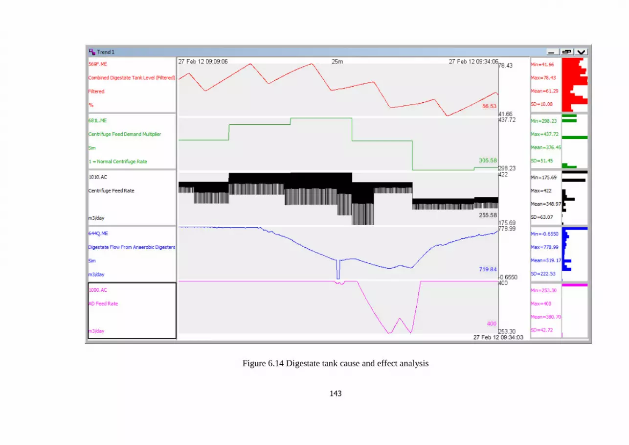
143
Figure 6.14 Digestate tank cause and effect analysis

144
Figure 6.15 CHP feed rate cause and effect analysis
Change in 696P.ME before change in observed in other
signals
Change is observed in other signals
with delay

145
Figure 6.16 Ambient temperature effect on digester temperature

146
CHP feed rate: Figure 6.15 shows plots of CHP feed rate speed in blue top plot,
followed by the gas holder level in green, digester temperature in purple and the heating
water circuit temperatures (before the AD, after CHP and after the coolers) in black.
The plot shows that changes in CHP feed rate do not correspond well with setpoint
changes. Due to the high priority set for the controller objective and constraints to avoid
flaring biogas (shown in Table 6.5), as the gas holder level rises to its high constraint
level, the setpoint of the CHP feed rate is override to increase the flow to reduce the
level in the gas holder. Comparison with other related signals shows it corresponds to a
drop in the heating water circuit temperatures affecting the CHP feed rate.
Understanding of these cause and effect relationships has enabled better control
implementation to be achieved.
Ambient temperature: ambient temperature effect on digester temperature is
considerable as illustrated in Figure 6.16, with digester temperature in blue, ambient
temperature in red and digester feed rate in black. An increase of one degree in ambient
temperature increases the digester temperature by 0.089˚C. Ambient temperature is set
as a disturbance in the controller specification due to it being an environmental effect
which cannot be controlled or predicted. However by understanding an increase or
decrease change in ambient temperature effect the digester temperature, the digester
temperature can be controlled better by factoring in the effects of ambient temperature
with manipulated variables effecting temperature.
6.4.2 Bottleneck shift
Bottlenecks are defined in the simulation as processing steps which hinder optimum
digestion of sludge to high yields of biogas. Depending on what the hierarchy of control
objectives are, the bottle neck in the process shifts to different processing steps.
However the main bottleneck in the process is the thickened sludge tank. The level of
thickened sludge available for digestion determines the variability in AD feed rate and,
therefore, affects the downstream processes. This is a result of the main controller
objective set to prevent the AD feed flow tripping as a result of high gas holder level,
which means the AD feed flow is more dependent on the biogas level than the thickened
sludge level. By setting the main controller objective to avoid tripping the thickened
sludge flow to the AD, the bottleneck shift to the gas holder level. This is a typical
situation observed on all of the benchmarked sites as sludge inventory are generally
high which result in optimum digester feed flows yielding high levels of biogas. Due to
finite levels of CHP units, this result in biogas being flared when CHP units run at
147
optimum levels. This issue may be only resolved through increasing the capacity of
tanks as this is the approach taken at Blackburn to increase CHP capacity through an
additional an CHP unit. Nevertheless the optimisation question remains as to whether it
is possible to process the high sludge inventory without flaring gas or tripping the CHP
units at this capacity. At present, this does not appear to be possible due to the high
inventory levels and constraint on tank volumes, still there is a considerable reduction in
gas flaring for which the cost will be beneficial to operate in this manner and flare little
gas, rather than invest in increased tank capacity to the site such as additional CHP
units. This is of course subject to environmental regulations, as tighter control on gas
flaring will inevitably occur and increase the importance of avoiding gas flaring
objective in the system.
6.5 Controller results
Following an iterative approach to tuning and tightening the MPC controller, a series of
seven hour simulation runs were conducted to evaluate the system. Seven hours of
simulation time equates to about twelve weeks of ‘real-time’. The seven hour runs were
conducted for the series of scenario evaluation tests outlined in Section 6.5 which
includes:
Evaluating the MPC1 controller structure, results for this is given in sections
6.5.1 and 6.5.2;
Evaluation of the MPC2, results for this is given in Section 6.5.3 ;
Evaluating the optimiser on MPC1 controller, results for this given in Section
6.5.4;
PID controller evaluation and ‘uncontrolled’ scenario analysis is provided in
Section 6.5.5.
6.5.1 MPC1
The simulation process is bottlenecked in capacity just like the industrial processes
benchmarked in the feasibility study. Therefore for a given design and capacity
availability, optimum setpoints can be identified and only then can the process be fully
optimised. Due to the process continuing to be inhibited by capacity, the level of feed
into thickened sludge tank has to be reduced or the tank sizes increased to enable the
process to be optimised. Therefore the simulation can serve as a test bed for designing
new plants.

148
Through setting and tightening constraints on the thickened sludge tank level, the tank
level is maintained without tripping. The tanks increase AD feed rate to keep the tank at
the low level resulting in increased biogas production and led to the bottleneck moving
to the gas holder. As CHP units are run at maximum speed, increase of gas flaring
occurs.
The mean of the thickened sludge tank and the digester feed rate plot shown in Figure
6.12 are close to each other; 606 and 611 for the sludge tank feed and the digester feed
respectively considering the large ranges as indicated by the standard deviation which,
is 581.16 and 181.19 for 288Q.ME and 491P.ME respectively. The digester feed rate for
the purpose of stability and control needs to have minimum standard deviation. To limit
this gas holder level setpoint is kept to a minimum of 9 to avoid hitting the low
constraint setpoint of 8 which is required for maximum efficiency of the CHP operation.
Tighter control is required on the thickened sludge tank level due to the large
disturbance of incoming sludge to the site. Giving the tank lots of head room enables it
to accommodate variation when sludge availability increases and reduces as the changes
are very rapid over a large range. For this reason the tank level 332Q.ME is set as a soft
constraint with high and low constraint limits as 60 and 40 %, respectively. The tight
constraint limits enable the tank to adjust without hitting the levels where trips occur.
These tight constraint limits are required for ideal control of the industrial process.
The digestate tank level and centrifuge operation can be controlled fairly easily due to
the feed forward information from AD feed rate. Temperature is controlled very well
and this was expected as most industrial sites have reliable temperature control.
The key findings from the simulation assessment can be summarised as follows:
The feed to thickened sludge tank level i.e. the sludge inventory on site changes
quickly and is unpredictable, therefore prediction of incoming feed is not
possible. The aim was to implement disturbance profile modelling into the
controller design to help the controller better predict changes;
Temperature is best controlled by the feed rate for cooling with cold sludge feed
making heating more difficult as cold sludge is continuously added. The next
factor affecting temperature is the cooler or boiler settings followed by ambient
temperature and CHP speed respectively;

149
The best setpoints are identified to best control the process with constraints
settings based on system dynamics and process understanding.
With respect to the aims of this study, it is evident that an advanced controller such as
MPC can reduce the limitations of inventory for a constraint optimisation problem such
as this. This can be carried out through measurement accuracy, speed of response,
stability and relative stability and sensitivity. Process prediction is only as good as the
underlying model, then knowledge and account of eventualities and variability is
essential to maintaining effective control. Disturbances can be a result of change in
process dynamics, measurement noise or external factors.
In summary, the model predictive controller has been shown to significantly improve
the process. Best temperature settings for various scenarios are identified. An advanced
controller such as MPC can be used to effectively control the multi-constraint, nonlinear
characteristic of the process. The MPC calculates a future set of moves to avoid the
constraint violation. This has been shown to improve the process in a simulation
environment as shown in Figure 6.17; where about 40 % increase in biogas production
can be achieved at 13 % lower average temperatures.

150
Figure 6.17 Inventory improvement results

151
6.5.2 Cost benefit analysis of MPC1
The MPC1 model is further evaluated on cost benefit basis to quantify the financial
gain from the controller. There are costs benefit elements associated with several
parameters which are calculated by the simulation. These cost and benefit elements
were modelled into the simulation as shown in Figure 6.18 to yield the total
simulation cost benefit signal shown at the bottom of the plot in black. The cost and
benefit elements are:
1. Savings associated with CHP electricity generation, the benefit is calculated
based on the following energy tariffs, shown in the blue (top) in Figure 6.18. 4.6
p kWh-1
- before 07:00, 13.3 p kWh-1
- between 16:00 and 19:00 and 6.7 p kWh-
1 - any other time.
2. Cost associated with the thickened sludge silo tripping on a high level, resulting
in no sludge being imported onto site until the 'backlog' is cleared, therefore a
cost penalty of £1000 day-1
for 24 hours is applied. This is shown in green in
Figure 6.18.
3. Cost associated with the thickened sludge silo tripping on a low level is shown
purple in Figure 6.18. This requires the operator to do some work to clear the
trip and reset the plant, therefore a cost penalty is applied with the penalty of
£600 day-1
for four hours.
4. Cost of the digestate silo tripping on a high level leading to the operator having
to clear the trip and reset the plant, therefore a cost penalty of £600 day-1
for
eight hours is applied. This is shown in dark yellow in Figure 6.18.
5. £600 day-1
for six hours is applied to the gas holder tripping on a high level,
resulting in the operator doing some work to clear the trip and reset the plant.
This is shown in light purple in Figure 6.18.
6. £600 day-1
for six hours is applied the digestate silo trips on a low level. This is
shown in orange in Figure 6.18, with all the cost penalty elements tripping the
tanks acting in on or off mode.
7. Electrical energy cost associated with running the adiabatic coolers is shown red
in Figure 6.18. The conversion efficiency between electrical energy and thermal
energy is assumed to be 50 % and the benefit is calculated based on the energy
tariffs of 4.6 p kWh-1
- before 07:00, 13.3 p kWh-1
- between 16:00 and 19:00
and 6.7 p kWh-1
- any other time.

152
8. There is a fuel energy cost associated with running the backup boiler is shown in
blue (bottom) of Figure 6.18. The boiler running on distillate fuel oil.

153
Figure 6.18 Signals associated with ‘real time’ cost calculations

154
The cost and benefit elements of the system are evaluated through changes in the
temperature setpoint. This is because temperature crucially effects the benefits of the
system, namely biogas production as this is modelled with the biogas correction factors
shown in Table 6.1, 6.2 and 6.3 in Section 6.2.2 and also the cost elements associated
with cooling and controlling the system.
Mesophilic digesters generally operate around 35˚C with a range between 25-45˚C. The
optimum temperature varies depending on the feedstock composition (Monnet, 2003).
Overnight runs (7 hours of simulation time, equivalent to about 3 months of ‘real life’
time) of the simulation were conducted at temperatures between 25-40˚C. The aim was
to evaluate best temperature condition for the operation of the simulation at set
conditions with the hypothesis that the optimum is around 35˚C.
Table 6.6 shows a summary of results from 14 overnight runs showing the effect of
temperature variation on the number of trips as previously listed in Table 6.4, CHP
energy savings and total simulation cost benefit analysis. The analysis of the trips
included:
1. The number of trips occurring – calculated from number of times any of the
level trips occur;
2. % of time trips occur – this is calculated as the % time taken to reset the level
trips;
3. GBT trip on high thickened sludge tank level (H TsT);
4. AD trip on low thickened sludge tank level (L TsT);
5. AD trip on high digestate tank level (H DigestT);
6. Centrifuge trip on low digestate tank level (L DigestT);
7. Flare on high gas holder level (H GHL);
8. CHP trip on low gas holder level (L GHL);
9. AD feed trip on high gas holder level (H GHL).
Together these 9 analyses of the trips together with the savings achieved by the CHP
unit yield the total simulation cost benefit analysis on the basis of the hierarchy of
control objectives and constraints set in Table 6.5.
Table 6.6 shows that lower temperature settings i.e. below 28˚C operate at a cost and
higher temperatures produce benefit for the system and therefore the digester should be
run 35 and 38˚C. This reflect the temperature effect on biogas production modelled with

155
a biogas correction factors shown in Table 6.1, 6.2 and 6.3 in Section 6.2.2, and follows
a parabola distribution as shown in Figure 6.20.

156
Table 6.6 Cost benefit associated with temperature
Temperature
(˚C)
No.
of
trips
% time
of trips
occurring
CHP
energy
savings
Total
simulation
cost
benefit
GBT
Trip
on H
TsT
AD
Trip
on L
TsT
AD trip
on H
DigestT
Centrifuge
Trip on L
DigestT
Flare
on H
GHL
CHP
trip on
L
GHL
AD
feed
trip on
H
GHL Run 1 25 513 101.7 538.6 -2297.17 197 0 88 0 0 228 0
Run 2 26 483 94.9 582.03 -2445.9 199 0 87 0 0 193 0
Run 3 27 425 86.3 643.6 -2379.14 203 0 88 0 0 134 0
Run 4 28 362 78.2 696.1 -2364.27 203 0 87 0 0 70 0
Run 5 29 322 75.9 740.56 -2340.86 207 0 90 0 2 30 0
Run 6 30 293 72.9 799.93 -2319.04 202 0 88 0 1 0 0
Run 7 31 395 49.9 1307.9 -255.56 347 0 0 0 32 0 16
Run 8 32 395 50.8 1413.32 -11.38 338 0 0 0 35 0 22
Run 9 33 430 54.1 1449.15 -27 354 0 0 0 44 0 32
Run
10
34 455 60.8 1441.74 -193.7 332 0 0 0 84 0 39
Run
11
35 691 65.8 1440.63 -391.87 350 0 0 0 291 0 50
Run
12
36 1533 77 1452.89 -483.05 383 0 0 0 1073 0 77
Run
13
37 1529 75.7 1465.67 -910.59 365 0 0 0 1092 0 72
Run
14
38 1101 70.9 1465.61 -2732.98 327 0 0 0 738 0 46

157
Analysis of the baseline analysis of the simulation performance without the
controller showed an average biogas production of 13,500m3 day
-1 as shown in
Figure 6.19, a CHP energy saving of £973 day-1
and all the seven level trips shown
in Table 6.4 tripping. With the controller active, CHP energy saving is increased to
£1,465 day-1
and the lower levels of the baseline only show low temperatures below
30˚C. If this average is maintained throughout the year, there is a saving of £492
day-1
, equating to approximately £179k a year. The cost to implement a control
project at Perceptive Engineering Ltd had two elements, the software and the
engineering services. The software generally cost around £12,000 for a “small” site,
and £18,000 for a “large” site, although this varies between projects. The cost for
engineering services varies also and generally the more manipulated variables, the
greater the estimated cost. For a site similar in size to the simulation, this would be
of the cost of £45k; making the total cost of the controller £63k. For this cost, the
payback time for installing the controller would be less than 6 months.
Figure 6.19 Biogas produced
Although the controller is shown to increase CHP energy savings by up to 33 %, real-
time optimisation and multivariable control systems typically add 6-10 % value to
process (Cutler and Perry, 1983). This is therefore a large saving on the CHP units. The
total cost benefit monetary value achieved for the simulation gave negative cost values
as shown in blue in Figure 6.20. The plot shows the cost benefit value achieved for
temperatures between 25 and 30°C is constant. The shape of the plot between 30 and

158
38°C however shows a bell curve or normal distribution plot with a peak at 33°C. The
negative values indicate that the plant cost money and made no profit with the
controller. However the negative values were a result of high cost penalties associated
with tripping the tank levels. The baseline simulation without the controller resulted in a
total cost of £2,135 day-1
. By setting the baseline as a zero cost benefit value and the
shifting the actual cost benefit values up by £2,135; Figure 6.20 also shows the shifted
total simulation cost benefit in red. This therefore gave highest cost benefit value for the
system at about £2,100 day-1
.
Figure 6.20 Total simulation cost benefit
There is constant benefit up to 30˚C before a large positive increase at 31˚C as shown in
Figure 6.20. The plot shows the optimum cost benefit gain to be around 32 to 33˚C.
This is again at the lower end of the mesophilic specification. The plot also shows total
benefit in £ day-1
to be below zero at all temperature settings. From the industrial data,
this is not true of AD systems as the process generates positive revenue. This is a result
of the cost elements built into the simulation design, where the balance of energy
produced revenue and cost associated with tank trips are not at the correct settings,
though the shape of the curve is valid for AD systems and changes in the cost values
will only shift the plot up. The revenue calculation does not also take into account
ROCs (renewable obligation certificate), which doubles the value of energy produced
on ADs.
-3000
-2000
-1000
0
1000
2000
3000
25 26 27 28 29 30 31 32 33 34 35 36 37 38
shifted Total simulation
cost/benefit
Temperature °C
C
o
s
t
/
b
e
n
e
f
i
t

159
Figure 6.21 illustrates the various trips occurring for the overnight runs at different
temperatures. From the results it is clear that for the temperature range of 25 to 38°C
studied using MPC1, the trips on the AD for the low thickened sludge tank level and the
centrifuge trip on high digestate tank is totally eliminated by the controller. Therefore,
the main issues for the overnight runs are the trips on high thickened sludge tank level
and the AD trip on high digestate tank level. This means that the level of inventory
coming into the site may be higher than what the plant is capable of processing. The
other level trips reflect the temperature effects on gas production as at low temperatures,
the CHP trip on low gas holder level occurs whilst at high temperatures; gas is flared
and the AD trip on high gas holder level occurs. This is expected due to the temperature
effect on biogas production modelled with a biogas correction factors shown in Table
6.1, 6.2 and 6.3 in Section 6.2.2. However the level of trips is greater at high
temperatures and should be avoided as the trips occurring at high temperatures may be
of greater cost due to gas flaring and tripping the CHP.
Figure 6.21 Number of trips
Figure 6.22 shows a plot of CHP energy savings against temperature settings between
25 to 38˚C. This shows a steady linear increase between 25 and 30˚C followed by a
large increase in CHP energy savings between 30 and 31˚C of about £510. The plot
illustrates that the peak energy saving is at 33˚C and this temperature setpoint was
related to the gas flaring at high temperatures and therefore increasing the temperature
above 33°C does not significantly increase CHP energy savings.
0
200
400
600
800
1000
1200
25 26 27 28 29 30 31 32 33 34 35 36 37 38
No
. o
f T
rip
s o
ccuri
ng
Temperature ºC
100.ME GBT Trip on H TsT
104.ME AD trip on H DigestT
110.ME CHP trip on L GHL
108.ME Flare on H GHL
112.ME AD feed trip on H GHL

160
Figure 6.22 CHP energy savings against temperature
Figure 6.23 Number of trips occurring versus temperature
Figure 6.24 % of times trips occur
500
700
900
1100
1300
1500
25 26 27 28 29 30 31 32 33 34 35 36 37 38
CH
P E
ner
gy S
avin
gs
(£)
Temperature ºC
200
400
600
800
1000
1200
1400
1600
25 26 27 28 29 30 31 32 33 34 35 36 37 38
No
. o
f T
rip
s O
ccuri
ng
Temperature ºC
40
50
60
70
80
90
100
25 26 27 28 29 30 31 32 33 34 35 36 37 38
% o
f T
ime
Tri
ps
Occ
uri
ng
Temperature ºC

161
Figure 6.23 and Figure 6.24 shows the give number of trips occurring and the % of time
trips occur. There is high level of trips occurring around 36 to 37˚C resulting from trips
in the gas holder leading to gas flaring. This is due to the increase in high gas
production resulting from the high temperatures. The gas is being flared because the
CHP units have reached their maximum capacity. Figure 6.23 also show the temperature
settings where minimum trips occur. This is highlighted by the black circle between 31
and 32°C setpoints. The % of time the trips occur shown in Figure 6.24 is also lowest at
these setpoint. This is, therefore, the best setpoints for achieving lower levels of trips
occurring at the lowest amount of time.
The key findings from the simulation assessment can be summarised as follows:
Significant reduction in level trips, with total elimination of AD trip on low
thickened sludge tank level and centrifuge trip on low digestate tank level;
A key setpoint in the process is around 31˚C, where the level trips are at zero, or
stable. Total simulation cost benefit and CHP energy savings increase
significantly above 31˚C;
Optimum temperature for total simulation cost benefit gain was found to be
around 33˚C instead of the predicted optimum of 35˚C. This is specific to the
simulation conditions, as sludge inventory is high, high temperature operations
incur more trips and the cost element associated with these within the simulation
makes operation at high temperatures not cost effective. The optimum is
therefore process dependent as at different capacities and operational constraints,
the optimum will vary.
6.5.3 MPC2: System dynamics
This section reviews the results for the MPC2 controller depicted in Figure 6.8. This
controller was designed to investigate the benefits of separating the slow and fast
dynamic parameters in the simulation as AD system has varying dynamics.
On observing the controller in the simulation, it became evident that the slow dynamic
structure was too slow to react to the changes in the fast dynamics structure and effected
the rate of response in meeting the controller objectives. This can be demonstrated in
Figure 6.25. The plot show gas holder level (purple) has fast dynamics and is affected
by biogas production which is affected by digester temperature (blue) and feed rate
(green). As the gas holder level increase to the point of tripping the level, the feed rate
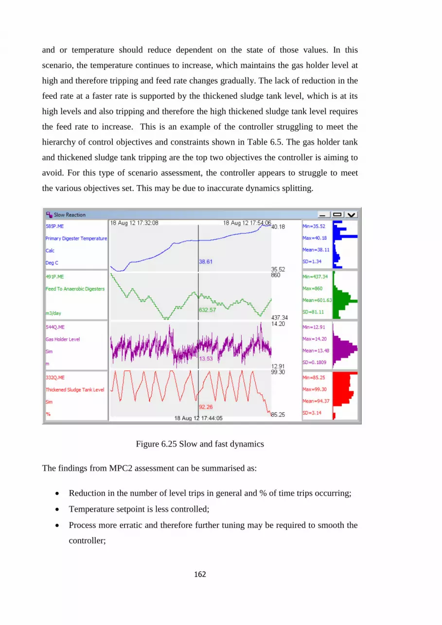
162
and or temperature should reduce dependent on the state of those values. In this
scenario, the temperature continues to increase, which maintains the gas holder level at
high and therefore tripping and feed rate changes gradually. The lack of reduction in the
feed rate at a faster rate is supported by the thickened sludge tank level, which is at its
high levels and also tripping and therefore the high thickened sludge tank level requires
the feed rate to increase. This is an example of the controller struggling to meet the
hierarchy of control objectives and constraints shown in Table 6.5. The gas holder tank
and thickened sludge tank tripping are the top two objectives the controller is aiming to
avoid. For this type of scenario assessment, the controller appears to struggle to meet
the various objectives set. This may be due to inaccurate dynamics splitting.
Figure 6.25 Slow and fast dynamics
The findings from MPC2 assessment can be summarised as:
Reduction in the number of level trips in general and % of time trips occurring;
Temperature setpoint is less controlled;
Process more erratic and therefore further tuning may be required to smooth the
controller;

163
Gravity belt thicker trip on high thickened sludge tank tripped above 197 times
for all MPC1 simulation runs, however for the MPC2 model; this is reduced to
77. Which is over a 60 % reduction in the number of trips occurring for the GBT
system;
The overall simulation cost benefit did not improved for the settings.
Although the findings show that the MPC2 simulation system is less controlled
smoothly in comparison to the MPC1 structure, there is a significant reduction in the
number of level trips occurring in the system. Further assessment can be conducted on
this model to ascertain whether any further improvements can be made.
6.5.4 Optimisation
A quadratic programming (QP) optimiser discussed in Section 4.3.1 and 4.3.3 is applied
to the MPC1 structure in Figure 6.7 and evaluated. The first objective of the QP
optimiser is to keep the process within the bounds of its constraints followed by cost
minimisation.
Figure 6.26 Controller Management page of flat structure with optimiser
For comparison purpose; all optimum settings for the MPC1 structure were kept as
shown in Figure 6.26, depicting the controller management page with the optimiser

164
switched on. When the QP optimiser is active, the solution is ‘relaxed’ in most cases.
This happens when the QP cannot find a feasible solution within the defined constraint
limits, therefore the constraint limits are allowed to be ‘relaxed’ according to the
priority settings that have been provided (Perceptive Engineering Ltd, 2012). This
means the solution provided is not the optimum operating point of the process but a best
attempt was carried out to satisfy the constraints and priorities. QP ‘relaxed’ output or
infeasible solution may be due to model errors or incorrect model set-up.
Figure 6.27 Tighter control achieved with optimiser
The result from the optimiser showed tighter control is obtained with temperature values
deviating less than 0.5˚C. Although constraints were violated at some reduced instances,
the optimiser appears to control the process well as shown in Figure 6.27. The figure
shows primary digester temperature (purple), feed rate (blue), thickened sludge tank
level (red) and gas holder level (green). As the thickened sludge tank reduces close to its
low limit level trip, the feed to the AD gradually reduces to enable the thickened sludge
tank level to increase. A decrease in feed rate cause the gas holder level to reduce
further due to the low feed rate and this causes the temperature to increase to enable
more gas production.
6.5.5 Controller performance comparison
This section compares MPC1, MPC2 and the MPC1 with the optimiser PID controller
and the base model without controller. The best performing temperature setpoint for the
simulation was at 33ºC and thus the simulated results were at 33ºC. Figure 6.28 depicts

165
the CHP energy savings and total simulation cost benefit in £ per day. The results
favour the benchmark MPC1 controller shown in dark blue, which yields highest CHP
energy savings for the system and high total simulation cost benefit value. This is
followed closely by the MPC1 with the optimiser controller shown in light blue and
then the MPC2 (purple). The performance with a ‘no controller’ shown in red performs
better than the PID controller and although the ‘no controller’ yields £0 of total
simulation benefit to the system, the PID controller results in £510 cost.
Figure 6.28 Controller evaluation comparisons: CHP energy savings and total
simulation cost benefit
The benefit of the optimiser on MPC1 was evident on comparing the number of trips
and the % time of time the trips occur. There appears to be a significant reduction in the
number of level trips occurring with the MPC1 and optimiser as shown in Figure 6.29 in
dark blue. The figure shows a reduction in trips with the optimiser for up to 92 % less
from the ‘no control’ benchmark simulation system. This is a significant finding and
may help formulate the case for implementing an optimised solution for the actual
industrial application for the project.
MPC2 plotted in red is shown to outperform MPC1. This is a significant finding as
MPC2 was shown to have 60 % and 63 % reduction in level trips and % of time the
trips occur respectively, whilst MPC1 was shown to have 38 % and 49 % reduction in
level trips and % of time the trips occur respectively. There separating the various
-510
-10
490
990
1490
1990
CHP energy savings Total simulation cost/benefit
£ p
er d
ay
MPC1+ Optimiser MPC1
No Control PID
MPC2

166
dynamics in the simulation enables reduction in level of trips. However MPC2 yields
lower energy savings and total benefit than MPC1.
Figure 6.29 Controller evaluation comparisons: No. of trips and % time of trips
occurring
Although the PID controller yields 2 % reduction in level trips than the ‘no controller’,
the PID controller takes longer to reset itself as shown in Figure 6.29 purple with the
longest % of time the trips occur. The 2 % in level trips can potentially increase by
developing multiple PID controllers on the system. However the reduction in level trips
did not reflect the CHP energy savings and the overall cost benefit of the system. This
may be due to the values given to certain cost elements within the model. For example,
priority settings and actuator move weights were tuned to ensure low levels of trips
occur as the primary aim of the simulator. Therefore the simulator aims to limit the level
of tank trips before optimising CHP energy savings and biogas production to improve
the overall cost benefit of the simulator.
6.6 Discussions and conclusions
The inventory simulation was subject to several assumptions and therefore the results
presented here have to be treated with caution. There is however significant evidence
0
100
200
300
400
500
600
700
800
No. of trips % time of trips occuring
No
. a
nd
% o
f ti
me
trip
s o
ccu
rin
g
MPC1+Optimiser MPC2
MPC1 PID
No Control

167
that an advanced controller such as MPC can significantly reduce the number of level
trips; as per the scenarios tested in the analysis.
The simulation results illustrate that the multi-objective control problem of AD can be
controlled with respect to scheduling and inventory. The simulation also highlights the
problems associated with the system dynamics. The large variability in the system
means variables such as temperature settings take a considerable time to heat or cool
down with the boiler cooler settings whilst the cooling effect on increased feed is more
instantaneous. Therefore the benefit of separating the dynamics in MPC2 has been
shown to significantly reduce the number of level trips occurring.
There remain significant trips still occurring in the system, especially for the MPC1,
which were mainly due to the system capacity to cope with the high sludge inventory.
The degree of improvement with respect to control and efficiency of the process
controllability is subject to the design. Capacity plays a detrimental role, as findings
from all benchmarked sites showed a bottleneck resulting from the inventory. This had
led to AD systems being historically designed at larger scales than operational intent. In
spite of this, these processes are still subject to capacity limitations. With respect to the
AD consortium for this project, this was an area where better understanding is required
for future designs. The design limitation issue cannot easily be removed and companies
cannot continue to design larger plants than needed for operation to enable better
flexibility for inventory and scheduling due to economic factors. The aim therefore is to
apply better control and optimisation solutions to improve the process and reduce the
limitation of capacity. This will be achievable not just through better monitoring but
increased and combined understanding of the various areas of the process. Strong
integration of microbial, bio-physiochemical and engineering for improving the
economics of the process will yield better improvement of the control of AD processes.
The existing control system at Blackburn WwTW is reduced to temperature and level
controls. The benchmark study showed that this level of control was not efficient for
controlling the process; however the data available lacked capturing of the system
dynamics for modelling for control implementation. The simulation here is used as a
basis to evaluate the specific dynamics, correlations and relationships needed to design
controllers for a potential system. This would require plant testing or formally DoE to
yield robust data for modelling. Future activities following on from the assessment

168
conducted so far therefore includes plant testing to generate data robust enough for
constructing models as per the simulation to evaluate the MPC1, MPC2, MPC1 plus
optimiser and PID controllers for controlling inventory and optimising the AD system
as a whole.
Generating robust data for modelling requires instruments that can measure the required
parameters capturing the dynamics, correlations and relationships within the system. In
some such cases robust instrumentation was unavailable and as such opportunities for
inferential measurements were investigated. Chapter 7 is an example of such
investigation which aimed to test the capability of building volatile solids inferential
sensor model.
169
7 Volatile solids model
7.1 Introduction
Lack of instrumentation is the main control bottleneck in the AD process. Sensors and
analysers are necessary to reduce the variability related to changes in the initial
conditions, uncertain kinetics and input concentrations of the process. Without
knowledge of the process conditions, the process is inevitably difficult to control.
Inferential measurement is a powerful and increasingly popular methodology that
allows process quality and difficult to measure process parameters to be inferred from
other easily measurable parameters such as temperature, flows and pressures. This study
investigates the opportunities for developing inferential sensor for volatile solids (VS).
7.2 Digestate
Traditionally, the objective of AD in wastewater treatment plants (WwTP) has been that
of sludge stabilisation and odour reduction. Biogas production, solids destruction and
pathogen reduction are now key areas of interest with biogas being the main product.
The second by-product, digestate, is the solid component that remains after digestion,
and is typically used for agricultural purposes or sent to landfill. Digestate quality is
thus becoming more important with industry exploiting it as a valuable end-product.
The availability of instrumentation for the monitoring of digestate quality is limited and
generally offline. Risk-based management and control procedures are in place to
manage digestate quality, in particular where the intended use is agricultural land. The
quality of the digestate must comply with appropriate microbiological standards,
including the safe sludge matrix (SSM) (Davis et al., 2010). Digestate quality attributes
as defined by the Publicly-Available Specification 110 (PAS110) (WRAP, 2010) and
the SSM include the level of VS, volatile fatty acids (VFA), residual biomass potential
(RBP), animal by-product (ABP) and hazard analysis and critical control points
(HACCP) for compliance with declarations of pH, total nutrients (Nitrogen,
Phosphorus, Potassium), total solids (TS), and loss on ignition (WRAP, 2010) required.
PAS110 ensures that the AD system uses suitable input materials, which are effectively
processed to produce digestate product in sufficient time. The process must also be
managed and monitored to meet both market needs and for the protection of the
environment. The specification offers digestate producers guidelines for the AD
process, as industry accepted specifications for digestate and ADs are unavailable.

170
Process monitoring in the fermentation industry is well advanced and established. The
similarities of such processes are aligned with AD and therefore technological
developments in this area are interest to AD researchers. Process Analytical Technology
(PAT) enables monitoring of complex biological processes using electrochemical and
spectroscopic instruments. By applying PAT with chemometric multivariate data
analysis to the AD process, it could ensure the optimum potential of the AD process to
reach new levels of stability, robustness, reliability and effectiveness (Madsen et al.,
2011).
Chapter 2 and 3 demonstrated the strong requirement for increased robust
instrumentation, for the AD process, which is the main bottleneck in process control
improvement. There is a strong interest to characterise the quality of digestate but to
date, there is no set specification for digestate quality. SSM and PAS110 are used as
guidelines to meet HACCP compliance. Therefore the availability of an online digestate
quality attribute through the use of PAT and chemometric multivariate analysis would
enhance the control of digestate quality and could potentially increase the value of the
digestate.
Biosolids is the term used to describe the treated solids fraction of the digestate or
stabilised sewage sludge (Lawrence K; Wang et al., 2008). The safe sludge matrix
(Chambers et al., 2001) governs the regulation for applying sewage sludge on
agricultural land. This is supported with processing requirements, storage and
application procedures to reduce the risk to human health and the environment. The
stability of the digestate is defined by several factors such as the level of pathogens,
odour and reduction in further decomposition of the organic materials involved (Gomez
et al., 2005). There is no single accepted analytical method to measure this multi-
attribute stability factor. However there are several individual tests to define the degree
of stabilisation. Digestate as a quality output measurement of the digestion process is
dependent mainly on feed sludge composition, digestion temperature and retention time.
The process greatly depends on influent feed composition and therefore in order to
model digestate quality, knowledge of the feed composition is required. The quality test
for digestate is based on test for stability, test for compliance and declaration of other
quality variables. These are:
VS;

171
VFA (0.43g COD gVS-1
);
Residual biomass potential (RBP) 0.25l gVS-1
;
Animal by product (ABP) and HACCP compliance;
Declaration of pH, total nutrients (Nitrogen, Phosphorus, Potassium), TS, loss
on ignition.
The compliance element is based on the digestion conditions of temperature and
retention time and is the main aim during digestion to meet the HACCP requirement.
This requires digesting the sludge for a set period of time at a set temperature dependent
on the characteristic of the feed stream.
Total solids (TS) measure the solids in the digestate and are composed of insoluble
suspended solids (SS) and soluble compounds. Volatile solids is the main organic
fraction which can be burnt off from the SS (Alturkmani, 2010). The quality of digestate
is defined by the organic and inorganic matter present, in the absence of phytotoxicity
and weed seeds.
The key parameters affecting digestate quality are temperature and retention time (Seadi
and Holm-Nielsen, 2010). However due to the highly variable feed compositions in the
feed and feed flow, these parameters may affect digestate quality immensely. The
digestion process offers valuable nutrient source as the process generally enhances the
availability of nutrients. Characterisation of digestate quality requires the stability
factors and declaration of the pH and nutrients to be modelled. Analysis of the nutrient
content is very important, as it affects the price for selling digestate. This is calculated
from the sum of nutrients (N, P2O5 and K2O) available to plants for land application.
Provided there are measurements for these variables, the digestate quality can be
calculated. Chapters 2 and 3 demonstrated current methods for measuring digestate are
limited to irregular, infrequent and offline measurements of % DS and volatile matter.
Instrumentation for measuring digestate quality parameters as determined by pH are
readily available and implement on industrial scale AD systems. Control of nitrogen
removal rate and phosphate precipitation are measured (Ingildsen, 2002), where N, P
and K nutrient values are measured offline. VFA sensors are available on pilot scale and
information for industrial scale application is not available. Residual biomass potential
can also be calculated offline. There are testing procedures for all these variables as part

172
of the PAS110 criteria (WRAP, 2010). Table 7.1 highlights the test procedures and
requirements for digestate quality measurements.
Table 7.1 Digestate quality test procedures
Test Method Test
period
Accuracy or
reproducibility
RBP Measure of stability by measuring the
total biogas production within a specified
period of time, at 35˚C
28 days Affected by high VFA
concentrations
VFA Online instrumentation available for
AnaSense, Capilex etc. methods include
wet chemistry methods of distillation,
colorimetric technique, titration and gas
chromatography such as the Shimadzu
GC-2010 (Shimadzu, 2012).
Minutes Weak concentrations are
difficult to detect,
accuracy increases with
high concentrations.
VS Commonly two step drying method by
heating the sample to about 105˚C to dry
off the water, the weighted dry cooled
sample is then dried further at 550˚C to
dry off the VS
About 7
hours
Affected mainly by the
temperature and drying
time.
7.2.1 Volatile solids
Volatile solids are organic compounds found in animals and plants. The biological
digestion process of AD breaks these solids down and converts into CH4, CO2 and H2
etc. Volatile solids in the digestate is determined by the % DS fed into the digester, the
sludge composition, digestion temperature and the % DS of the digestate. VS is
analysed by drying a sample of the digestate in high temperature ovens. This is an
important digestate quality output test for stability and the % VS remaining in the
digestate will eventually break down post digestion and potentially pollute the
environment (through land application as biosolids). High VS content in the digestate
means fewer solids are converted into biogas during digestion and therefore results in a
173
waste of resources. There is therefore an economic and environmental reason for
reducing the level of VS in digestate. Measurement of VS enables a quantitative
measure of the organic matter but fails to account for biodegradability of the solids in
the digestion process. Therefore high VS (low degradation) levels post digestion may
indicate process inefficiency or the presence of organic matter like lignin which are not
biodegradable (Schievano et al., 2011). VS destruction rate is inevitably affected by
many factors to including level of polymer added, digester operating temperature,
mixing efficiency, retention time, characteristic of the microorganisms available,
composition of sludge etc. These factors make the VS measure difficult in both
prediction and estimation.
VS provide an indication of the stability of the digestate and hence the stability of the
process can be inferred. Online instrumentation for VS is not available and, although
offline analysis can be conducted, the sampling rate is typically low and irregular. VS
may potentially provide a better indication of the sludge quality (biochemistry) than
other measurements such as % DS (Dry Solids Percentage). It is expected that VS will
negatively correlate with biogas production, as an increase in biogas corresponds to an
increase in the breakdown of organic molecules and therefore lower VS. The effect of
temperature on VS may be more complex due to the non-linear relationship between
temperature overall process performance. In general an increase in temperature from
mesophilic to thermophilic increases the reaction rate and efficiency at which the
organic solids are destroyed resulting in a lower VS (Buhr and Andrews, 1977). A
negative correlation can be expected between VS and retention time, with VS having
been shown to decrease with increasing retention time (Moen et al., 2003).
Measurement test procedures for VS are also simpler than those conducted offline for
VFA or RBP, as the test for VS does not require wet chemistry techniques such as
titration, colorimetric and chromatography techniques as required for VFA (Palacio-
Barco et al., 2010). For these reasons, VS is an important digestate quality attribute and
the use of VS for online monitoring and control will potentially result in a tighter
control on digestate quality.
7.2.2 Soft sensor use in AD systems
The behaviour of a process is indicated by the measurements made and are related to the
state of the process. Information contained in many secondary variables reflects the
behaviour of the primary variables. Therefore, the aim of this study is to investigate
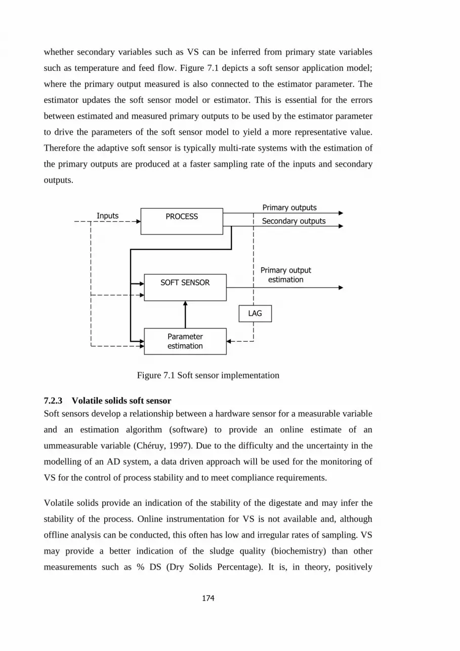
174
whether secondary variables such as VS can be inferred from primary state variables
such as temperature and feed flow. Figure 7.1 depicts a soft sensor application model;
where the primary output measured is also connected to the estimator parameter. The
estimator updates the soft sensor model or estimator. This is essential for the errors
between estimated and measured primary outputs to be used by the estimator parameter
to drive the parameters of the soft sensor model to yield a more representative value.
Therefore the adaptive soft sensor is typically multi-rate systems with the estimation of
the primary outputs are produced at a faster sampling rate of the inputs and secondary
outputs.
Figure 7.1 Soft sensor implementation
7.2.3 Volatile solids soft sensor
Soft sensors develop a relationship between a hardware sensor for a measurable variable
and an estimation algorithm (software) to provide an online estimate of an
ummeasurable variable (Chéruy, 1997). Due to the difficulty and the uncertainty in the
modelling of an AD system, a data driven approach will be used for the monitoring of
VS for the control of process stability and to meet compliance requirements.
Volatile solids provide an indication of the stability of the digestate and may infer the
stability of the process. Online instrumentation for VS is not available and, although
offline analysis can be conducted, this often has low and irregular rates of sampling. VS
may provide a better indication of the sludge quality (biochemistry) than other
measurements such as % DS (Dry Solids Percentage). It is, in theory, positively
Primary output
estimation
Secondary outputs
Primary outputs Inputs PROCESS
SOFT SENSOR
Parameter
estimation
LAG

175
correlated with feed rate and negatively correlated with temperature, retention time and
gas production.
VS are affected by a number of factors that are important to consider for modelling
purpose:
A higher temperature is shown to increase the speed of degradation and hence
higher temperatures may result in lower VS levels;
The digester feed rate determines the retention time, and organic loading rate
(OLR). By increasing the feed rate, the retention time is reduced and therefore
the sludge spends less time in the digester resulting in higher VS levels
potentially (Ponsá et al., 2008);
Feed composition is the main disturbance affecting VS levels, as digester biogas
and digestate depend on the composition of the incoming sludge. This includes
the level of VS entering the digester and the composition of the organic
compounds and microorganisms, and is therefore the primary source of
variability and the main disturbance (Ashekuzzaman and Poulsen, 2011);
Environmental factors such as pH, mixing and microorganism population also
affect VS. Antagonism (the suppression of some species of micro-organisms by
others), acclimation (adaptation to a new environment or a change to the old
environment) and synergisms (micro-organisms acting together for mutual
benefit) together can affect the level of VS that remains after digestion (Chen et
al., 2008).
Assuming linear relationships exist, these factors can be captured by the Equation VS =
Ax + By + e; where A is the OLR of the system, B is the temperature, x are the
unmeasured disturbances entering the system, y are the environmental factors including
pH and mixing and e is the error. Challenges faced in the development of a VS soft
sensor are associated with the unmeasured disturbances and the other unknown
environmental factors associated with microorganism activity.
To date there is no evidence of the application of a VS soft sensor. The reasons for lack
of studies into VS soft sensor development and commercial availability of robust online
instrumentation for VS are the same for other parameters such as VFA and % DS. These
reasons can be grouped into two (1) reasons within the industry (specifically water

176
industry where AD systems are more common) and (2) difficulty in designing of robust
instruments for treating bio-products such as digestate.
7.3 Blackburn AD volatile solids soft sensor development
Data from Blackburn WwTW anaerobic digestion process is used as the industrial data
for use in the VS soft sensor development study. The soft sensor development procedure
is outlined in Figure 4.6. These steps are common to most data based modelling
techniques with steps 2, 3, and 4 being the most important stages for getting a good
model. The availability of ‘good data’ is dependent on:
Sensor availability: The ‘right’ parameters being measured, having the right
instruments available to get the required data;
Accuracy and validity of the measurement systems: for evaluation of systematic
errors;
Precision and reliability of the measurement systems: to account for random
errors;
Sensitivity and dead band of measurement systems.
Sampled at the right rate and or frequency to capture the dynamics within the
process.
These make the selection of ‘right’ data a key step to obtaining a good model.
Furthermore ‘good data’ is about process coverage also. This needs more thought
coming up with more science and appropriate what constitutes ‘good data’. If the initial
data going into the modelling procedure is not robust enough, then inevitably, it will be
difficult to obtain a robust predictive model using such data.
7.3.1 Data selection
The Blackburn dataset contains approximately 396 signals, collected within the time
range of 14 January 2010 13:00 to 14 July 2010 12:00, i.e. about 188 days. The data is
time-aligned with a sampling interval of five minutes. Screening of all 396 signals was
conducted to select both online and offline signals which may have effect on the VS of
the digestate. There are signals which may affect VS from the start of the process in the
primary settlement tanks where offline measurement such as chemical oxygen demand
(COD), ammonia and soluble solids to digestate analysis of % DS and volatile acids
(VA). Current data from Blackburn WwTW provide offline information for digestate
volatile matter (VS), pH, alkalinity, volatile acids (VA), and percentage dry solids (%

177
DS). These are laboratory data extracted approximately twice per week. These fail to
meet the requirements of the PAS110 directive and general assessment of digestate
value, which includes: digestate stability measurement for residual biomass potential
(RBP), data for the log kill (HACCP), and nutrient levels for Nitrogen (N), Phosphorus
(P) and Potassium (K). These are important for setting the price for the digestate, as per
the AD calculator.
The offline VS, VA, pH, and % DS may be used to estimate the quality of the digestate.
Modelling of all these parameters will require a multiple-input multiple-output (MIMO)
system that will be difficult to assess the quality of the digestate. In such cases,
experience indicates that, multiple multiple-input single-output (MISO) models are
preferable. The plan is therefore to develop a MISO system for modelling VS, pH or
VA. From the data provided there are several signals available for the development of a
possible soft-sensor. However most of these signals are only available offline. Online
signals that may be useful in developing the soft sensor include:
Digester liquid and foam levels and flows;
Polyelectrolyte usage;
EH hydrolyse stage temperature in and out;
Pasteurisation stage temperature in and out;
Digester gas produced and pressure;
Digester temperature.
There are different levels of measurements for the different processing units as depicted
in Table 7.2. There are mixing and buffering tanks before or after each stage. The
sampling time at each point therefore reflects the measure of the variable at the time and
therefore temperature in the hydrolysis phase, is not a measure of the same sample in
the digester at any particular point. Thus the measurements need to be time aligned. The
sludge preparation area has few online signals but some useful offline signals regarding
sludge composition. Data from this area will be excluded as all the feed stream is
entered into the buffer tanks and continuous feed of the mixed sludge is fed to the
thickening phase. Although there are good online data for the thickening stage, as a
means of reducing variability in the system, the thickened sludge is entered into a buffer
tank before feeding into the EEH, thus the tanks act as filters as well as delays. Without
any details of the lag time for the thickening stage, the data cannot be time shifted to

178
reflect the digestion process. This is true for the other processing steps except the EEH
stage which is known to take 1.5-2 days and therefore can be shifted to match VS. For
this reason data selected for the modelling are extracted from the EEH and digestion
phase alone. However the sludge flows from the EEH is split into the 4 digesters and
there are irregularities as at times the total flow is directed towards one single digester.
For these reasons, the EEH data is also excluded from the analysis. This leaves only
variables during the digestion phase, for which due to limited instrumentation, most of
the key parameters needed to characterise VS are unavailable, these include pH,
alkalinity, VFA and sludge composition.

179
Table 7.2 Signal availability for different processing units
Sludge
preparation
Thickening EEH Digestion Digestate
Process
function
mixing imported
food and sewage
sludge with sites
own sludge
Removal of excess water and
polymer addition to yield % DS
between 6-8 %
Separates hydrolysis and acidogenic
stages from methanogenic stage.
Inactivates pathogen, optimise process
and reduce RT.
Stabilisation of sludge,
gas production and
pathogen reduction
Digestate cake
preparation process.
Main
Processing
units
BAFF, sumps, grit
removal, storage
units
Gravity belt thickener, polymer
dosing unit, air mixing and
thickened sludge buffer tank
3 serial CSTR’s at 42˚C, 3 serial batch
tanks at 55˚C and 2 water sludge or
water HEX
Adiabatic cooler, 4
digesters
Polymer dosing
unit, centrifuge, 3
buffer centrate
balancing tanks
Online
signals
Flows Sludge fed through thickener, poly
usage. Unthickened sludge, buffer
tank level, energy cost or usage and
volume
Thickened sludge flow in or out, tank
level, boiler circuit temperature,
hydrolyser or pasteurisation stage
sludge temperature in or out, foam
levels, energy cost and usage
temperature, pressure,
temperature, sludge
flow, gas produced,
foam depth and liquid
level
Levels, flow, cake
pile level, centrate
speed, poly dosing
flow or usage
Offline
signals
Ammonia, BOD,
COD, SS. 16 tank
levels
Ammonia, BOD, COD, pH, VS, %
DS
None None H2S, % DS, SS,
alkalinity, pH, VA,
VM
Average
process
duration
Continuous Continuous 2 days 14 days continuous
Mode of
operation
Continuous Continuous Batch or Continuous Continuous Continuous
Processing
effects on
VS
Feed composition
and sludge age
Concentration of polymer, initial
VS and % DS will have significant
effect on final VS
Temperature, hydraulic residence time,
feed rate, and mixing will significantly
affect VS
Temperature, feed rate,
retention time and
mixing will significantly
affect VS
Not applicable

180
7.3.2 Data Pre-processing
The process data generated is generally very noisy; as it contained a lot of errors,
missing data and outliers it therefore required various pre-processing techniques to
refine the data. The systematic pre-processing procedure is:
Handle missing data;
Outlier detection;
Data alignment;
VS offline data pre-processing to reflect the online data;
PCA.
Figure 7.2 Data selector use to remove missing data
There are large sections of data missing in the signals due to a possible power or
operational failure as shown in pink on Figure 7.2. Due to the large level of missing
data, the data selector was used to remove the data completely from the analysis. On

181
visual inspection of time series plot of the missing data, it was evident that some of the
samples were outliers or errors. In Figure 7.3, plot of retention time for primary digester
1 is shown as 570D.ME. On the plot there is a signal peaking at 867.47 days for
retention time. This is a clear error as normal operating range for retention time is
between 20 to 25 days or less for EEH digesters. Removal of the missing data and
extreme outliers resulted in selection of 88.2 % of the data for analysis (these are signals
that equal 1 on the data selector signal) with 11.8 % of the data removed.
Figure 7.3 Signals post data cleaning and signal shifts
Outlier detection is one of the initial steps in data analysis for obtaining a coherent data
set. It is common that what may be seen through visual inspection as noise or error may
not be necessarily bad data and that these outliers can carry important information about
the process. As such removal of what may be deemed to be as outliers can lead to a
model giving incorrect results, misspecification and biased parameter estimation (Ben-
Gal, 2005). The univariate hampel filter (Hampel, 1971; Hampel, 1974) addresses the
issue outliers have on the robustness of an estimator. The hampel filter approach was
then used to remove further outliers such as the spikes in feed and gas data.

182
Figure 7.4 Volatile solids signal from process data showing actual and pre-processed
signals
Figure 7.4 depicts plot of the VS signal from the process data where the top blue plot is
the actual signal and bottom red is the pre-processed signal. The offline VS data has 50
samples over the whole 6 months period of data collected compared to 17280 samples
for the online signals. The offline signals are extracted 2 to 3 times per week and there
are various factors affecting the sampling and analysis which needs to be taken into
consideration, such as:
Multiple sampling points: the sample can be extracted from different points
dependent on which pump is in use;
Sampled amount for analysis varies: an accurate measure of the analysis sample
is not conducted but judged from experience. The initial weight is noted and the
final weight is taken from it to give the loss in weight due to VS. It is evident
that drying times effect VS values, the variation in weight can effect the drying
time and therefore yields inaccurate measurement of VS;
Operator variation;
Data entry: the calculated VS values are entered into the PI historian system
from which there can be errors, especially in matching the time stamped against
the time the sample is taken;

183
Control: there is little evidence of operator retraining or management systems to
ensure tests are carried out correctly.
These sampling and analysis issues suggest a poor level of accuracy in the VS data. As
a consequence the data may not capture the dynamics or give a full of account of VS in
the digester.
Figure 7.5 Observation of effects of sludge flow on retention time and temperature
Volatile solids are affected by temperature and the retention time. Both these parameters
are controlled by the digester feed. This makes the digester feed the most important
cause attribute. The feed controls the process in general; however the signal operates in
an on or off mode and as such required averaging of the data over a 12 hour period. The
correlation between the variables is useful to consider. Increase in temperature causes a
reduction in VS levels yielding a negative correlation, however the observed correlation
in Figure 7.5 is the opposite, as there is a positive correlation. This arises due to
problems in time alignment. The data is shifted to align the observations, in order to
capture the uncertainties in the lag times such as the time taken for an increase in
temperature to take an effect on volatile solids. This was conducted through visual
inspection of the data to identify patterns which may identify the cause-effect

184
characteristics of the process. Misalignment in the data also resulted in cause signals to
act as effect signals with respect to VS and therefore data alignment was key to the
model building.
Table 7.3 Initial correlation analysis
Peak correlations VS Temperature RT Feed flow
VS 1 -0.543 -0.557 0.547
Temperature -0.543 1 -0.548 -0.416
RT -0.557 -0.548 1 -0.285
Feed flow 0.547 -0.416 -0.285 1
In a theoretical sense, temperature, retention time and feed flow depicted in Figure 7.5
should have significant effect on VS and therefore should be highly correlated with VS.
Table 7.3 summarises initial peak correlation analysis of VS against these parameters
conducted in PerceptiveAPC. By shifting the data sets and aligning the signals, the
expected peak correlation is achieved. From this initial analysis, the signs (±) of the
correlations are as expected; negative correlations for temperature and retention time as
increase in these factors reduces the level of VS and positive correlation for feed flow as
increases in the feed flow increases the VS levels. However the values of the correlation
values are weak, which may be because of the dynamic impact.
7.4 Modelling
A good quality model relies on the quantity and quality of the data used for the
modelling. It has been suggested that the input data must have minimum of 5 measured
changes with 5 times larger than the noise associated with the input (Boudreau and
McMillan, 2007). The historical data generated for the VS prediction model lacked this
characteristic and therefore a possible DoE may be required for improvement of the
quality of the data. Such a procedure involves conducting step or pseudo random binary
sequence (PRBS). The generation of such data may take months to years for a
bioreactor system such as the AD.
185
Chemometric methods of PCA and PLS are used in the modelling stage for obtaining
predictive model for VS. Given a set of data consisting of a large number of interrelated
variables, PCA aims reduce the dimensionality of the data set whilst retaining the
variation in the data set as much as possible (Jolliffe, 2005). Principal component
analysis (PCA) was developed in 1901 by Pearson (Pearson, 1901) with the geometric
optimisation explanation and later Hotelling in 1933 (Hotelling, 1933) with the
algebraic derivation of PCA. Principal component analysis (PCA) is popular procedure
for reducing the dimensionality of the variable space. The inferential sensor study uses
the PCA technique for examining the relationships within the AD process data. This has
a large number of measured quality variables of which most are highly correlated
therefore reducing the dimensionality of the multivariate data to a few manageable
dimensions. Importantly the original variables are retained as each principal component
is a linear combination of the original variables. This enables the representation of the
original data set containing correlated variables, in a new ordinate system that is
characterised by uncorrelated variables called principal components (PCs).
The procedure was carried out using Matlab software with the PLS toolbox (Wise et al.,
2010). The data was first autoscaled before applying PCA since the variables have
different units. As PCA aims to capture variation, autoscaling enables all variables to be
treated on an equal basis in the analysis and therefore variables that have greater
variation due to the magnitude of the variable do not dominate variables with smaller
order of magnitude of variation.
7.4.1 Correlation analysis
Correlation analysis on both offline and online signals which may have an effect on VS
was conducted, and the results shown in Figure 9. However most do not reflect the
impact on the sludge within the digester due to the different process stages. Most of the
signals showed have little or no correlation with VS, which could be due to time delays
within the processes. The opportunity to have VS predicted online within a short time
period is essential for control of the AD process. Therefore there was a need to establish
the time delays for the various cause signals. The effects of these parameters on VS is
not well established from first principles and as a result, the time taken for VS variable
to settle to steady state after a step change for parameters such as temperature, feed rate,
retention time or gas production cannot be determined theoretically. As a result an

186
iterative search was conducted to establish an appropriate min or max delays for the
model, and therefore the data shifted to align the cause and effect variables.
Figure 7.6 Signals Selected For Modelling
Figure 7.6 lists the signals available for modelling required for the VS soft sensor.
These are online signals that may affect digested sludge VS. This constitutes of 14
signals which required pre-processing before analysis to remove bad data caused by
missing values. The missing data approach is to replace bad values by the last good
value.
The data in general contained a lot of spikes and the measurement of the flow was
contaminated by opening and closing the valve, resulting in a repetitive irregular
pattern. To reduce this, spike removal analysis was conducted on the gas produced, and
the feed flow signal was averaged over an hour to reduce the on or off pattern in the
data.
The development of the soft sensor was conducted in two phases. Phase 1 required
analysis of the data to investigate which of the variables selected have a statistically
significant effect on the digested sludge VS. This was conducted using PCA and
response surface regression analysis in Minitab 16 Statistical Software. Phase 2 required
the use of the PerceptiveAPC PLS modelling solution to formulate a prediction model.

187
The online signals formed a large dataset which was too large for analysis in Minitab 16
Statistical Software. The VS offline signal holds the same data point for about 2-3 days.
The data was therefore reduced in size to reflect the changing VS data points only. The
46945 samples were therefore reduced to 67 samples. This considerable reduction in the
sample size will effect the results considerably but will allow better estimation of the
effects on VS.
Figure 7.7 Correlation analysis on various signals
The correlation analysis results in Figure 7.7 indicate overall weak correlations for all
the cause signals. These are peak correlations and some of the cause signals selected do
not just have little theoretical justification but also the delays and changes in the various
stages of the process mean that these cannot be used as direct effects. There were
several variables which were shown to correlate strongly with VS, such as foaming and
liquid levels. These variables may be related to other variables, for which the
relationship or correlation may be caused by another factor in the system such as the
sludge composition. Variables deemed to have a causation relationship with VS include
temperature and feed rate which also determines the retention time, but the correlation
values for these are much weaker than expected. The results here are therefore
insufficient for selecting these as cause signals for the prediction model and therefore

188
further analysis is required to select variables that can aid with building a theoretically
and industrially robust prediction model.
7.4.2 Parallel coordinates
Figure 7.8 Parallel coordinates plot A and B
Parallel coordinates plots conducted to explore relationships between different signals.
This is robust method for visualising and analysing multivariate data. The results given

189
in Figure 7.8 showed that high pasteurisation temperatures in and out of the EEH stage
correlate with low VS levels. This is a significant finding as high pasteurisation
temperature means the initial pre-treatment stage in the EEH has significant effect on
the level of VS. However the relationship is not a direct linear function as the pre-
treated sludge goes into a buffer unit before entering the digester. High levels of % DS
also infer high levels of VS, which is expected. Low levels of pH post digestion is
shown to yield low level of VS as digester pH is not available it can be assumed that by
keeping the digestion pH low, VS destruction rate may increase resulting in the low
levels of VS observed. However the range of pH post digestion is quite small between
6.9 and 7.6 and although most of the lower level of pH is observed for low VS, there are
high pH values for low VS as well. BSM2 simulation environment may give further
insight into pH effect on VS and this is to be investigated further.
7.4.3 Minitab 16 Statistical Software response surface regression analysis
Hypothesis test analyses were conducted here to determine whether there is enough
evidence to reject or accept the null hypothesis. This was conducted using Minitab 16
Statistical Software (Microsoft-cooporation, 2006) and background to be covered in the
methodology section of the thesis.
Table 7.4 Estimated regression coefficients for VMPD
Term Coef SE Coef T P
Constant 56.353 0.8117 69.425 0.000
Foam Level -3.079 1.1942 -2.578 0.012
Liquid Level -5.680 1.6086 -3.531 0.001
Dig1Temp 2.104 1.0257 2.052 0.044
The final results from this analysis showed the factors that have statistical significance
to VS were foam level, liquid level and temperature in the digester. These factors have
P-value <0.05 and are shown in Table 7.5. P-value is an estimate of the probability that
the results occurred by accident. That is there is lee than 5 % chance that the results
were by chance. Temperature is expected to have significant effect on VS as high
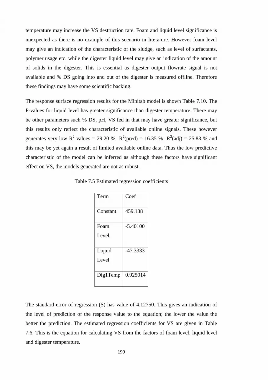
190
temperature may increase the VS destruction rate. Foam and liquid level significance is
unexpected as there is no example of this scenario in literature. However foam level
may give an indication of the characteristic of the sludge, such as level of surfactants,
polymer usage etc. while the digester liquid level may give an indication of the amount
of solids in the digester. This is essential as digester output flowrate signal is not
available and % DS going into and out of the digester is measured offline. Therefore
these findings may have some scientific backing.
The response surface regression results for the Minitab model is shown Table 7.10. The
P-values for liquid level has greater significance than digester temperature. There may
be other parameters such % DS, pH, VS fed in that may have greater significance, but
this results only reflect the characteristic of available online signals. These however
generates very low R2 values = 29.20 % R
2(pred) = 16.35 % R
2(adj) = 25.83 % and
this may be yet again a result of limited available online data. Thus the low predictive
characteristic of the model can be inferred as although these factors have significant
effect on VS, the models generated are not as robust.
Table 7.5 Estimated regression coefficients
Term Coef
Constant 459.138
Foam
Level
-5.40100
Liquid
Level
-47.3333
Dig1Temp 0.925014
The standard error of regression (S) has value of 4.12750. This gives an indication of
the level of prediction of the response value to the equation; the lower the value the
better the prediction. The estimated regression coefficients for VS are given in Table
7.6. This is the equation for calculating VS from the factors of foam level, liquid level
and digester temperature.

191
A B
Figure 7.9 Contour Plots for VS against Foam Level, Liquid Level and Digester
Temperature
The contour plots depicted in Figure 7.9 shows that from the design high levels of foam
and liquid level is required to obtain low VS levels at low temperatures. High liquid
levels may mean that the level of solids may be low in the digester and therefore lower
VS. This may be the reason for the strong statistical significance. Correlation with foam
level is not so strong. From the contour plots in Figure 7.9, there is not a clear best
operating domain by which the 3 factors of temperature, foam and liquid level can be
operated to ensure low VS and therefore high gas production etc. From Figure 7.9a, low
VS level at most is associated with low temperatures, although temperature spread is
quite wide and high foam levels. The rise in foam level may be due to increase VS
destruction rate and therefore increase in reaction increase may constitute high foam
level and therefore low VS output. From plot B, low temperature effects on VS are
more visible and correspond with high liquid levels. In theoretical sense and therefore
the hypothesis expect high temperatures to correspond with low VS rather than low
temperatures. For these reasons, along with the weak predictive model generated, the
model has little scientific and process knowledge justification and therefore deem
unsuitable.
PCA was used here to establish the relationships between the data and samples or
identifying patterns within the data as shown in the 6 diagrams in Figure 7.10. The final
zoomed in plots in figure 13E and 13F reveal that feed rate, temperature and gas
produced show to be similar, closely grouped with VS and therefore related to the VS.
Dig1Temp
Foa
mLe
ve
l
34.534.033.533.032.532.031.531.030.5
9.4
9.2
9.0
8.8
8.6
8.4
>
–
–
–
–
–
< 45
45 50
50 55
55 60
60 65
65 70
70
VMPD
Contour Plot of VMPD vs FoamLevel, Dig1Temp
Dig1Temp
Liq
uid
Le
ve
l
34.534.033.533.032.532.031.531.030.5
8.25
8.20
8.15
8.10
8.05
>
–
–
–
–
–
< 45
45 50
50 55
55 60
60 65
65 70
70
VMPD
Contour Plot of VMPD vs LiquidLevel, Dig1Temp

192
7.4.4 Principal component analysis
PC1:PC2 plot B: zoomed in view
C:PCe:PC4 plot D: Zoomed in PC3:PC4 plot
E: PC1:PC2 Final F: final PC3:PC4 plot
Figure 7.10 PCA results of available signals
-0.4 -0.2 0 0.2 0.4 0.6-0.5
-0.4
-0.3
-0.2
-0.1
0
0.1
0.2
0.3
0.4
0.5
Loadings on PC 1 (59.77%)
Loadin
gs o
n P
C 2
(27.9
3%
)
470Y.ME
484Y.ME
498Y.ME
500Y.ME
570Y.ME
578Y.ME
634Y.ME
714P.ME
722P.ME 738P.ME 166P.ME
714P.ME
722P.ME
730P.ME 760P.ME
Variables/Loadings Plot
0.25 0.3 0.35 0.4 0.45 0.5
-0.2
-0.15
-0.1
-0.05
0
Loadings on PC 1 (59.77%)
Loadin
gs o
n P
C 2
(27.9
3%
)
498Y.ME
500Y.ME
570Y.ME
578Y.ME
722P.ME
738P.ME
166P.ME
722P.ME
730P.ME 760P.ME
Variables/Loadings Plot
-0.5 0 0.5 1-0.6
-0.4
-0.2
0
0.2
0.4
0.6
0.8
Loadings on PC 3 (4.45%)
Loadin
gs o
n P
C 4
(3.5
9%
)
470Y.ME
484Y.ME
498Y.ME
500Y.ME
570Y.ME
578Y.ME
634Y.ME
714P.ME
722P.ME
738P.ME
166P.ME
714P.ME
722P.ME
730P.ME
760P.ME
Variables/Loadings Plot
-0.2 -0.15 -0.1 -0.05 0 0.05 0.1 0.15 0.2
-0.15
-0.1
-0.05
0
0.05
0.1
0.15
Loadings on PC 3 (4.45%)
Loadin
gs o
n P
C 4
(3.5
9%
)
470Y.ME
484Y.ME
498Y.ME
500Y.ME
570Y.ME
578Y.ME
634Y.ME
714P.ME
722P.ME
738P.ME
166P.ME
714P.ME
722P.ME
730P.ME
760P.ME
Variables/Loadings Plot
-0.8 -0.6 -0.4 -0.2 0 0.2 0.4 0.6 0.8-0.6
-0.4
-0.2
0
0.2
0.4
0.6
0.8
Loadings on PC 1 (82.42%)
Loadin
gs o
n P
C 2
(15.9
8%
)
470Y.ME
484Y.ME
570Y.ME
578Y.ME 738P.ME
Variables/Loadings Plot
-0.8 -0.6 -0.4 -0.2 0 0.2 0.4 0.6 0.8-0.5
0
0.5
1
Loadings on PC 3 (1.16%)
Loadin
gs o
n P
C 4
(0.4
5%
)
470Y.ME
484Y.ME
570Y.ME
578Y.ME
738P.ME
Variables/Loadings Plot

193
7.4.5 Estimator modelling in PerceptiveAPC solution
Figure 7.11 Actual and pre-processed VS signal
Figure 7.11 shows actual VS signal in blue and pre-processed signal in red. Due to low
number of samples and the VS values being held until a new sample value is available,
peak position filtering was conducted on the data. This gives the best approach of filling
in the gaps in sampling. About 50 samples over the whole 6 months of data collected
compared to over 17280 for online data. Offline samples are extracted 2-3 times per
week from multiple points of sampling. Sample amount for analysis varies with focus
only in the loss of weight as the difference between the initial sample weight and final
weight after testing. Quality control of the analysis procedure is difficult to determine as
there is no documentation of re-training, or management system in place to ensure all
tests are carried out in similar manner. The values generated from the offline tests are
entered into the PI historian system; there is a chance of possible errors on inserting the
data back in the data historian. All analysis conducted are also subject to operator
variation, for these various reasons, the accuracy, precision and significance of the
offline VS data is difficult to determine. The data however covers a wide range of
values; with minimum and maximum value of 42.70 and 70.30 respectively, these give
acceptable VS and unacceptable VS results as per the PAS110.

194
Table 7.7 give the results for correlation analysis conducted in Matlab (Mathsworks,
2012). These values are very low and fail to provide quantify significant relationship
between the factors of feed rate, feed VS, temperature, pH and gas produced. With such
low correlation value, a weak predictive model will inevitable be resulted from these
value. The signs (±) of the correlation values fail to make scientific sense. Theoretically
as the feed rate increases, digestate VS should increases and therefore yield a strong
positive correlation as the sludge spends less time in the digester and thus lower
degradation process generated. However a weak negative correlation is observed. High
temperatures are expected to increase the degradation process and therefore more
organics are broken down, thus low VS resulting. Giving a strong negative correlation
instead of the weak positive correlation observed. This infers that as you increase the
temperature, VS values increases. Although this confirms the results from the Minitab
study, there is no scientific justification for it. This is also true for the gas production
effect on VS. As VS decreases, inferring that there is high degradation rate, this should
result in high gas production. Unexpectedly a positive correlation is observed where a
strong negative is presumed.
Table 7.6 Blackburn digestate VS correlation values
Digestate VS correlation
values
Feed
rate
Feed
VS
Temperature pH Gas
produced
Blackburn process data -0.2839 0.2884 0.4096 0.3247 -0.1663
Figure 7.12 shows the loading plot after shifting VS data for 1 day to correspond with
feed rate and temperature effects. 738X.ME is VS. Feed rate (484X.ME) positively
correlates with VS and Temperature (578X.ME) negatively correlates with VS. This
pre-processing helps to obtain the expected signage of correlation and higher correlation
values. Provided the dynamics in the system observed is correct and thus justification
for shifting the online data forward one day, then this shift in data may result in a better
predictive model which makes scientific sense to some degree.
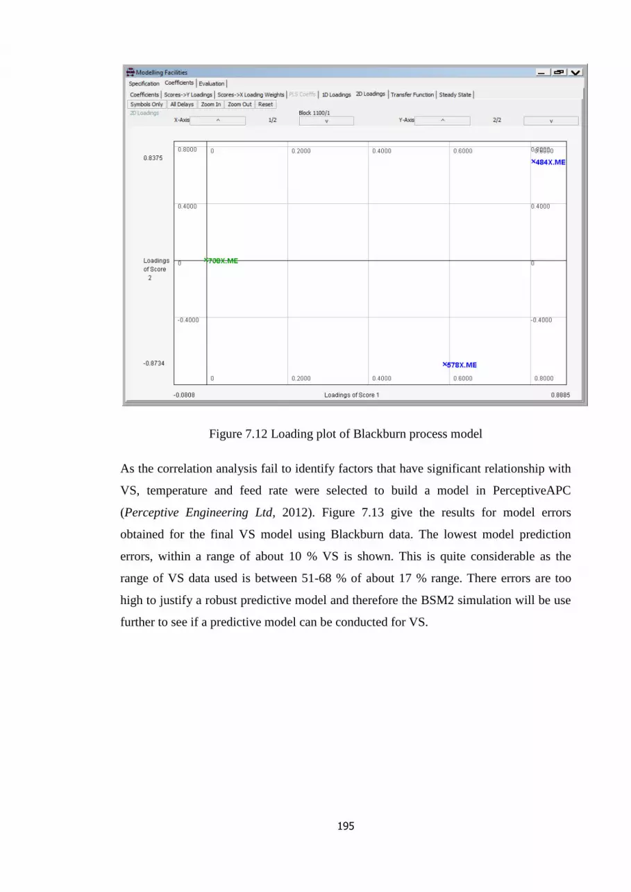
195
Figure 7.12 Loading plot of Blackburn process model
As the correlation analysis fail to identify factors that have significant relationship with
VS, temperature and feed rate were selected to build a model in PerceptiveAPC
(Perceptive Engineering Ltd, 2012). Figure 7.13 give the results for model errors
obtained for the final VS model using Blackburn data. The lowest model prediction
errors, within a range of about 10 % VS is shown. This is quite considerable as the
range of VS data used is between 51-68 % of about 17 % range. There errors are too
high to justify a robust predictive model and therefore the BSM2 simulation will be use
further to see if a predictive model can be conducted for VS.

196
Figure 7.13 Final process model errors
7.5 Volatile solids soft sensor development in ADMI
Benchmark systems are popular for the assessment of process performance i.e. biogas
yield, control system evaluation and comparison of similar purposes are common in
defining the best possible approach to take before implementation for cost reduction. A
wastewater treatment plant (WwTP) should be considered as a single completely
integrated system. This would enable primary and secondary clarification units,
activated sludge reactors, anaerobic digesters, thickeners, dewatering systems and other
sub-processes to be combined, operated and controlled by local and supervisory control
systems taking into account he interactions between the processes (Henze et al., 2008).
The European cooperation in science and technology (COST) Action 682 and 624
which ended in 2004 was set up with the aim of developing benchmark tools for
simulation based evaluation of control strategies for activated sludge plants. This work
is now continued under the framework of the IWA Task Group on Benchmarking of
Control Strategies for WwTPs. Together the group have developed:
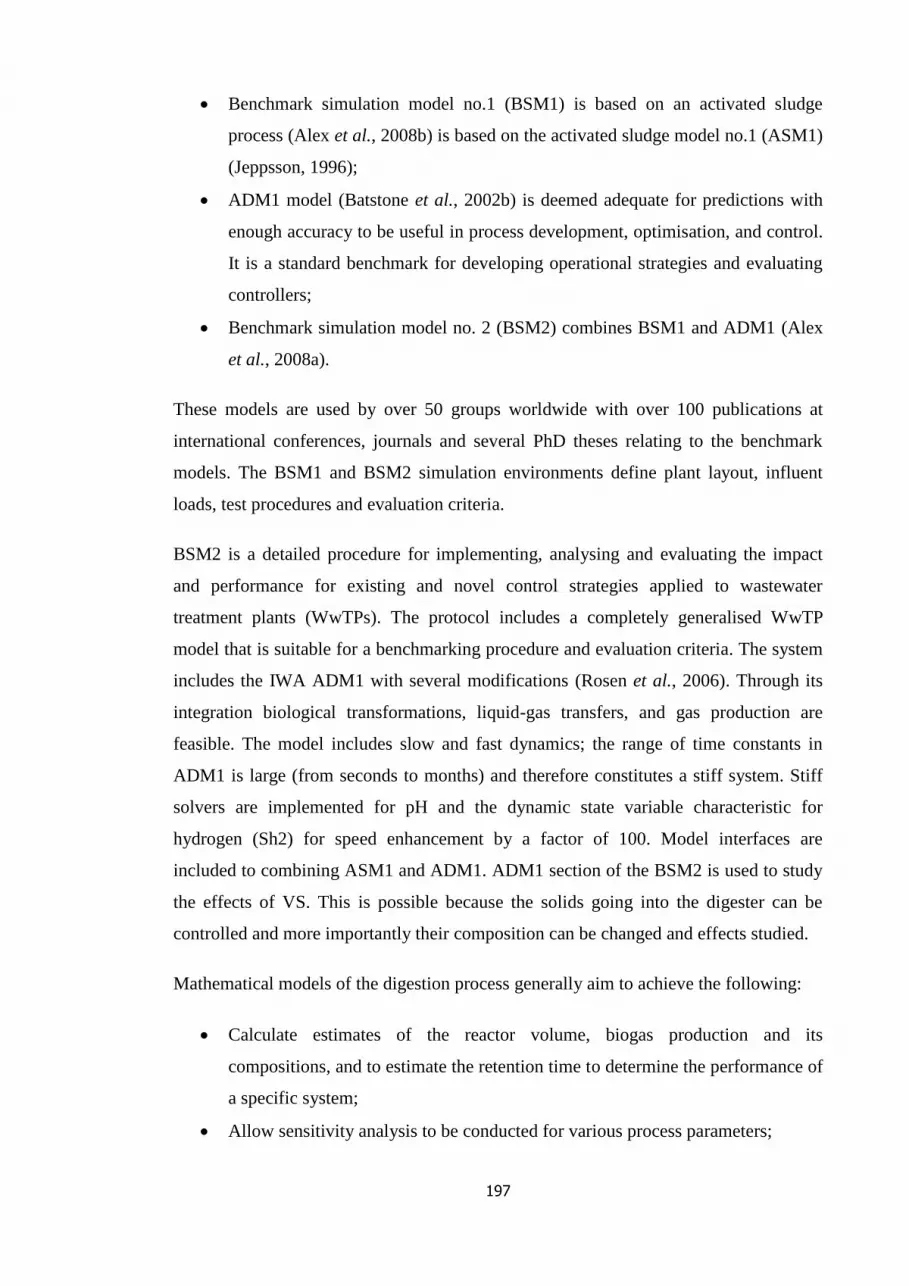
197
Benchmark simulation model no.1 (BSM1) is based on an activated sludge
process (Alex et al., 2008b) is based on the activated sludge model no.1 (ASM1)
(Jeppsson, 1996);
ADM1 model (Batstone et al., 2002b) is deemed adequate for predictions with
enough accuracy to be useful in process development, optimisation, and control.
It is a standard benchmark for developing operational strategies and evaluating
controllers;
Benchmark simulation model no. 2 (BSM2) combines BSM1 and ADM1 (Alex
et al., 2008a).
These models are used by over 50 groups worldwide with over 100 publications at
international conferences, journals and several PhD theses relating to the benchmark
models. The BSM1 and BSM2 simulation environments define plant layout, influent
loads, test procedures and evaluation criteria.
BSM2 is a detailed procedure for implementing, analysing and evaluating the impact
and performance for existing and novel control strategies applied to wastewater
treatment plants (WwTPs). The protocol includes a completely generalised WwTP
model that is suitable for a benchmarking procedure and evaluation criteria. The system
includes the IWA ADM1 with several modifications (Rosen et al., 2006). Through its
integration biological transformations, liquid-gas transfers, and gas production are
feasible. The model includes slow and fast dynamics; the range of time constants in
ADM1 is large (from seconds to months) and therefore constitutes a stiff system. Stiff
solvers are implemented for pH and the dynamic state variable characteristic for
hydrogen (Sh2) for speed enhancement by a factor of 100. Model interfaces are
included to combining ASM1 and ADM1. ADM1 section of the BSM2 is used to study
the effects of VS. This is possible because the solids going into the digester can be
controlled and more importantly their composition can be changed and effects studied.
Mathematical models of the digestion process generally aim to achieve the following:
Calculate estimates of the reactor volume, biogas production and its
compositions, and to estimate the retention time to determine the performance of
a specific system;
Allow sensitivity analysis to be conducted for various process parameters;

198
The cross-checking of simulation study results with actual plant performance
gives added knowledge about the model, and can identify gaps in the predictive
capability of the model;
Use in whole plant optimisation studies, as they can predict how the digestion
process is affected by upstream processes, and how the digestion process can
impact on downstream processes (Appels et al., 2008).
The ADM1 model is used here to compare and cross-check the result of the process data
VS model. As ADM1 is entirely theoretical, theoretical assessment of the process model
can be achieved.
7.5.1 Parameter evaluation in ADM1
Figure 7.14 Schematic of the simulation process
The schematic for the simulation process is shown in Figure 7.14. ADM1 is composed
of many several key measurement parameters such as VFA’s and sludge composition.
However there are several limitations within the model, such as:
Sludge characterized by proteins, carbohydrates and lipids only. This over
simplifies actual sludge characteristics;
Temperature effects considered for physiochemical parameters but not for the
biochemical reactions, temperature effects are not fully modelled;
Temperature cannot be varied within the simulation but able to conduct single
runs at different temperature settings between 0-60˚C;
Over simplification of the model and lack of temperature dependence means the model
greatly defers from actual AD processes. The complexities and nonlinearities within AD
processes are a mainly impacted by the feed composition and environmental factors of
temperature. ADM1 however offer several opportunities to include:
The organic compounds and inerts make-up the total solids. Therefore able to
add VS signal as a % of the organic compounds and the inert;
Thickener
MAD
Indigenous 1˚ and 2˚
sludge: characterised by proteins, carbohydrates,
lipids and inerts only
Biogas
Digestate downstream
processes

199
Opportunity to monitor VFA accumulation;
Opportunity to explore gas composition effects on changes to feed and VS.
With these opportunities, step tests can be conducted to generate data for modelling the
VS. although there are more key signals available in the simulation such as gas
composition and measure of the various VFA’s these are not available in the process
data and therefore, for model ‘like for like’ comparisons, these useful variables were
eliminated from the model. Thus an alternative model investigating the various
parameters available for modelling will be conducted to illustrate if with improve in
measurement; a better model can be generated with more variables.
𝑇𝑆𝑆 = 0.75(𝑋𝑆 + 𝑋𝐼 + 𝑋𝐵,𝐻 + 𝑋𝐵,𝐴 + 𝑋𝑃
Where XS is the slowly biodegradable substrate, XI is particulate inert organic matter,
XB,H as active heterotrophic biomass, XB,A as active autotrophic biomass and XP as
particulate products arising from biomass decay. These are the components measured in
the ASM1 domain to constitute solids going into the digester.
Table 7.7 COD Equivalent of polymer
Polymer Equivalent to COD
1g carbohydrates 1.07g COD
1g lipid 2.91g COD
1g protein 1.5g COD
The digester interface has these parameters converted to 3 main organic forms of
proteins, carbohydrates and lipids which make up the level of volatile solids measured
in kg COD m3-1
. The chemical oxygen demand (COD) is the amount of oxygen required
to oxidise the organic carbon completely to CO2 and water. COD contains both
biodegradable and non-biodegradable solids. COD measurements were converted into
VS through the following estimations for the simulation as shown in Table 7.8.
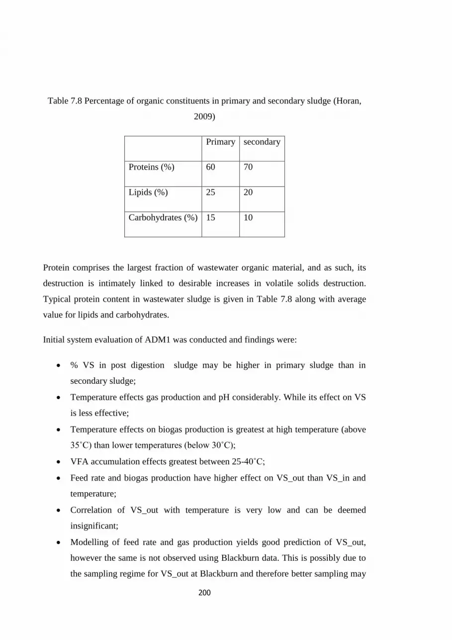
200
Table 7.8 Percentage of organic constituents in primary and secondary sludge (Horan,
2009)
Primary secondary
Proteins (%) 60 70
Lipids (%) 25 20
Carbohydrates (%) 15 10
Protein comprises the largest fraction of wastewater organic material, and as such, its
destruction is intimately linked to desirable increases in volatile solids destruction.
Typical protein content in wastewater sludge is given in Table 7.8 along with average
value for lipids and carbohydrates.
Initial system evaluation of ADM1 was conducted and findings were:
% VS in post digestion sludge may be higher in primary sludge than in
secondary sludge;
Temperature effects gas production and pH considerably. While its effect on VS
is less effective;
Temperature effects on biogas production is greatest at high temperature (above
35˚C) than lower temperatures (below 30˚C);
VFA accumulation effects greatest between 25-40˚C;
Feed rate and biogas production have higher effect on VS_out than VS_in and
temperature;
Correlation of VS_out with temperature is very low and can be deemed
insignificant;
Modelling of feed rate and gas production yields good prediction of VS_out,
however the same is not observed using Blackburn data. This is possibly due to
the sampling regime for VS_out at Blackburn and therefore better sampling may

201
provide data that can effectively illustrate the correlation of gas production and
feed rate on VS_out.
Step Testing
Step tests were carried out to test the system dynamics within BSM2. Some of these
results are depicted in Figure 7.15. There are mainly 4 signals going into the digester of
mainly the organic matter and inert. The total organic matter going into the digester is
assumed to undergo full disintegration with low residues. Therefore the volatile solids
are assumed to be the three polymers of carbohydrates, lipids and proteins. The
polymers plus the inert give the total solids going into the digester.
Table 7.9 Correlations analysis results for variables in ADM1
VS_out Feed rate VS_in Temperature pH Gas produced
1.0000 0.8945 0.7054 -0.0964 -0.4127 0.9306
1.0000 0.9440 0.7380 -0.0829 -0.4419 0.9713
Correlation coefficients of VS out against the 5 components selected and results are
shown in Table 7.9. First row for all data and second row data shows data for when the
process is in a stable state. As can be seen feed rate, VS_in, and gas produced all form
strong positive correlation with VS_out, while temperature and pH form weak negative
correlations with VS_out. The weak negative correlation with temperature is a
significant finding, as it demonstrates that initial assumption of VS_out being mostly
affected by the retention time and temperature mainly does not hold. And therefore VS
may be affected greatest by the feed rate, gas produced and the characteristic of the
incoming sludge i.e. the VS in. As feed rate and gas produced measurements are easily
available, makes these variables ideal for soft sensor model for VS_out. Correlation
coefficients values for gas flow and feed rate with VS_out:
Gas flow and feed rate both yields weak negative correlation with VS_out; this is the
opposite of what is observed in BSM2 where a strong positive correlation is observed;

202
This illustrates the weakness in the process data as it deviates strongly from what is
expected; however in theory VS_out should decrease with increasing gas production
and therefore the negative correlation is expected, but the value of the correlation is
very weak and therefore deemed insignificant to yield and accurate or reliable model.
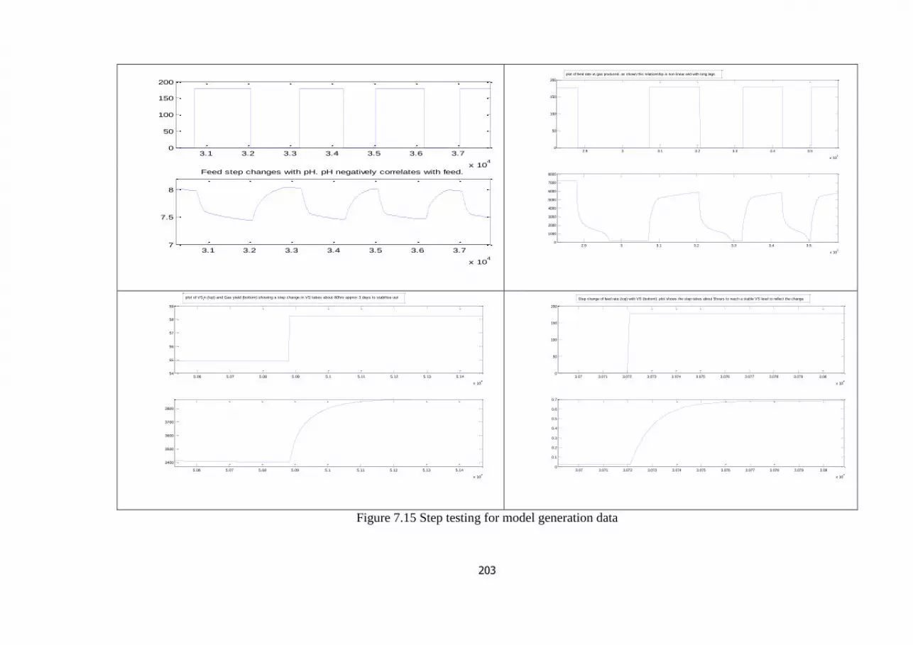
203
Figure 7.15 Step testing for model generation data
3.1 3.2 3.3 3.4 3.5 3.6 3.7
x 104
0
50
100
150
200
3.1 3.2 3.3 3.4 3.5 3.6 3.7
x 104
7
7.5
8
Feed step changes with pH. pH negatively correlates with feed.
2.9 3 3.1 3.2 3.3 3.4 3.5
x 104
0
50
100
150
200
2.9 3 3.1 3.2 3.3 3.4 3.5
x 104
0
1000
2000
3000
4000
5000
6000
7000
8000
plot of feed rate vs gas produced. as shown this relationship is non linear and with long lags.
5.06 5.07 5.08 5.09 5.1 5.11 5.12 5.13 5.14
x 104
54
55
56
57
58
59
5.06 5.07 5.08 5.09 5.1 5.11 5.12 5.13 5.14
x 104
3400
3500
3600
3700
3800
plot of VSin (top) and Gas yield (bottom) showing a step change in VS takes about 80hrs approx 3 days to stabilise out
3.07 3.071 3.072 3.073 3.074 3.075 3.076 3.077 3.078 3.079 3.08
x 104
0
50
100
150
200
3.07 3.071 3.072 3.073 3.074 3.075 3.076 3.077 3.078 3.079 3.08
x 104
0
0.1
0.2
0.3
0.4
0.5
0.6
0.7
Step change of feed rate (top) with VS (bottom): plot shows the step takes about 5hours to reach a stable VS level to reflect the change
204
Figure 7.16 ADM1 PCA loadings plots
The PCA loadings plot of the simulated data in Figure 7.16 shows that gas produced
rate and feed rate are similar to digestate VS. This is because on the loadings plot,
variables ‘sitting together’, grouped closely infer similar behaviour between variable
and thus maybe statically related. This analysis along with the correlation results
indicates that a good predictive model can be generated for VS with feed and biogas
flowrate alone. The benefits of selecting these two variables include:
Feed flow and biogas flowrate measurements available online;
Instrumentation for these are robust and readily available;
Use off primary input (feed flow) and primary output variables;
Feed flow is the main disturbance into the system and biogas flowrate a good
monitoring parameter.
The structure of the final model is therefore depicted in Figure 7.17. However a
successful model with feed and biogas flowrate alone will refute the understanding of
the multivariate characteristic of the process. However the various model assumptions,
over simplification of the process and the lack of temperature dependency inclusion in
the model may simply linearize the model and thus the process and therefore reducing
the multivariate characteristic of the process.
-0.6 -0.4 -0.2 0 0.2 0.4 0.6 0.8-0.6
-0.4
-0.2
0
0.2
0.4
0.6
0.8
Loadings on PC 1 (61.88%)
Loadin
gs o
n P
C 2
(25.5
0%
)
Feed_rate VS_in
Temperature
VS_out
pH
Gas_prod
Variables/Loadings Plot
-0.6 -0.4 -0.2 0 0.2 0.4 0.6 0.8 1
-0.2
0
0.2
0.4
0.6
0.8
1
Loadings on PC 3 (9.32%)
Loadin
gs o
n P
C 4
(3.1
8%
)
Feed_rate
VS_in
Temperature
VS_out
pH
Gas_prod
Variables/Loadings Plot

205
Figure 7.17 VS model
The results from the final model using feed and biogas flowrate to predictive VS is
shown in Figure 7.18. The first depict the results for the model in red and model errors
in blue. The model errors are very small and therefore a good predictive model is
generated.
Figure 7.18 VS predictive model from ADM1 results
7.6 Conclusions
The correlations of the variables with digestate VS in the industrial data are all very low
and not sufficient to yield a reliable process model. Gas flow and feed flowrate both
display a weak negative correlation with digestate VS. This result illustrates the
limitations of the process data as it deviates strongly from theory and the simulation
study. The low correlations observed may be a result of disturbances in the process
which are unmeasured and therefore not included in the model. This may include the
feed composition for which there is no measure and the environmental conditions in the
digester.
Utilizing the simulation data for the modelling of feed rate and gas production yields a
good prediction of digestate VS, however the same is not observed using the process
Property Predictor
Process response parameters
Feed flow rate
Biogas flow rate Volatile solids inferential sensor
Simple robust sensors
0 1 2 3 4 5 6 7 8
x 105
-1
0
1
2
3
4
5
6x 10
-3
yin(1:729231,1)
data 1
0 1 2 3 4 5 6 7 8
x 105
-2
-1.5
-1
-0.5
0
0.5
1
1.5
2x 10
-3
results.error

206
data. This is possibly due to the sampling regime at this site for digestate VS, sampled
approximately 2-3 times per week. Better sampling may provide data that demonstrates
a correlation between gas production and feed rate, and digestate VS. Analysis of the
simulation data revealed that variations in concentrations of VS in the range of 30˚C and
35˚C are very low. In the industrial data, the temperature ranged between 29˚C to 36˚C,
indicating that the range measured may be too limited to reveal the effects of
temperature on VS.
There is very little studies on digestate and measure of stability with respect to VS.
Initially analysis conducted confirms the digester environmental conditions of
temperature, levels of liquid and foam have statistical significant effect on VS of
digestate. The signals that may be better at characterising the digestate quality includes
with respect to VS include online data for:
% DS;
Feed type or composition;
pH;
Retention time.
However these signals are not available online. The model may improve significantly
provided there is possible online analysis for % DS and pH. The data available along
with the ADM1 simulation environment give the following findings:
Good prediction obtained with simulated data;
The relationships of process variables illustrated with PCA, VS more similar to
feed rate and gas production than temperature;
Deviation of correlation in process data from theoretical expectation, possibly
due to various unmeasured overshadowing effects;
The complexity of the underlying non-linearity in the system evident.
The correlation analysis of variables with digestate VS in the industrial data are all very
low and insufficient to yield a reliable process model. Gas flow and feed flowrate both
display a weak negative correlation with digestate VS. This result illustrates the
weakness in the process data available as it deviates strongly from theory and
simulation. The low correlations observed may indicate disturbances in the process
which are unmeasured and therefore not included in the model. This may include the
207
feed composition for which there is no measure of and the environmental conditions in
the digester.
Utilizing the simulation data in the modelling of feed rate and gas production yields a
good prediction of digestate VS, however the same is not observed using the process
data. This is possibly due to the sampling regime at this site for digestate VS, sampled
approximately 2-3 times per week. Better sampling may provide data that demonstrates
a correlation between gas production and feed rate, and digestate VS. Analysis of the
simulation data revealed that variations in concentrations of VS in the range of 30˚C and
35˚C are very low. In the industrial data, the temperature ranged between 29˚C to 36˚C,
indicating that the range measured may be too limited to reveal the effects of
temperature on VS.
The process data in this case study was unable to produce a model suitable for the
prediction of VS. The use of the BSM2 model however provided useful information on
the dynamics of the anaerobic digestion process. The next stage of this study will use
this knowledge to conduct a DoE study on the industrial process. The objective of this
DoE study will be the generation of data that covers the wide-ranging dynamics of the
system to help build an industrial VS soft sensor.

208

209
8 Conclusions
8.1 Introduction
This chapter concludes the thesis by returning to the research questions stated in
Chapter 1:
Can an advanced control system improve the efficiency, stability and robustness of an
AD process?, what is the minimum instrumentation requirement to achieve the aims
identified in the feasibility assessment? and what is the level of improvement to be
gained from advanced control?
Subsequently contributions and conclusions are summarised, followed by a perspective
for future work.
8.2 Discussions
This thesis has encompassed a feasibility study into the use of MPC on industrial AD
systems. This has included the benchmark study of four industrial processes, literature
search and instrumentation review identifying minimum, essential and ‘nice to have’
instrumentation, which formed the completion of phase I activities as set out in Figure
1.1.
The phase I activities aimed to address the first question “Can an advanced control
system improve the efficiency, stability and robustness of an AD process?” The
literature and instrumentation reviews identified the strengths, weaknesses opportunities
and threats for an advanced control such as MPC on industrial AD systems. These
findings along with the benchmark study formed the basis for the hypothesis that
“advanced control system can improve the efficiency, stability and robustness of an AD
process”. The thesis then progressed to demonstrate how an advanced control system
can improve the efficiency, stability and robustness of an AD process. The first step for
demonstrating the hypothesis was to identify the minimum instrumentation required to
for an MPC controller to fulfil the aims identified in the feasibility study. The
instrumentation review and the benchmark study identified key instrumentation
requirement. Parameters with readily unavailable instrumentation to monitor them
online were investigated further through the development of inferential sensor models to
predict parameters.
Chapter 7 investigated the VS soft sensor development activities respectively. This
chapter concluded that although there were significant improvements to be made with

210
regards to online instrumentation for industrial AD systems, soft sensor models offer
possible solutions that negate the need for expensive and potentially problematic online
measurements.
Following on from this the simulation study in Chapter 6 has shown the level of
improvements that are to be made with MPC. Through the inventory simulation
analysis, the hypothesis that significant improvements in the efficiency, stability and
robustness of the AD process can be made with MPC was proven true. This was
demonstrated at simulation level and not industrial scale. Therefore, it was deemed
necessary that the findings from the simulation and soft sensor models underwent
further investigation at industrial scale.
The industrial data used for the models in this thesis were not intended for MPC
modelling and the data provided have several limitations. The data used were taken
from systems where controllability and control model development approaches were not
considered at the design stages. Failure to adequately consider controllability and
control at the design stage means that any proposed control scheme is restricted by the
design. The AD system is subject to considerable uncertainties and disturbances that
affect the operating conditions and product qualities such as biogas and sludge
composition. To help achieve optimum dynamic performances and economic profits,
assessment of the performance with respect to controllability is required at the design
phase (Ekawati and Bahri, 2003). Measurements such as separation of the different
process phases for the digestion technology help improve the stability and
controllability. This reduces the degree of non-linearity in the system yet there still
remains an opportunity for improved control.
Although the inventory simulation demonstrated the level of improvements to be made
with MPC, there still remained analysis of the potential improvements that could be
made on real AD systems. The benchmark study data was shown to be insufficient for
modelling the effect of MPC using industrial data and as such various data sets from
different AD systems were analysed to test their usefulness for model development for
soft sensors and or MPC. A case study was conducted to show the use of sludge
composition data for VFA modelling. The case study focused on an analysis of data
generated in the School of Civil Engineering and Geosciences, Newcastle University.
The data relates to an experimental study of various feed compositions and includes an
analysis of the microbial population which provided an insight into the effects of feed
composition on the microbial and environmental conditions within a digester. The
211
objective of this case study was to combine the use of multivariate techniques with the
process knowledge developed through phase I and II activities and develop an
inferential sensor for predicting molecular species population changes to infer stability
of the AD process. A second case study was also conducted for the analysis of two
datasets obtained from (1) a laboratory for the treatment of wastewater from the starch
industry and (2) a pilot plant set-up for the treatment of waste water from the production
of bioethanol. The datasets were obtained from the Leibniz University of Hanover at the
Institute for Sanitary Engineering and Waste Management. The aim of this case study
was to compare different experimental setups of varying feedstocks and use of the data
for potential soft sensor or MPC models. A third case study was a comparison of two
datasets from different reactor design systems treating the same waste. The reactors
were the same size and are fed with same feedstock over a three month period. The
objective of this case study was to investigate the impact of different reactor systems.
These case studies combined the aims to investigate the impact of varying feedstocks,
reactor systems and experimental set-ups to understand how these changes effect the
dynamics within the AD process and where possible inferential sensor development was
conducted with case study datasets. However due to the limited results obtained from
these three case studies, they have not been included in the thesis.
8.3 Conclusion
In summary the main conclusions of this thesis are as follows:
1. MPC controller on a simulated AD system has yielded significant improvements
for controlling inventory, yielding:
40 % increase in biogas production can be achieved at 13 % lower
average temperatures;
£179k a year of CHP energy savings can be achieved, equating to 33 %
increase in CHP energy savings using MPC1. This could contribute to
the cost of installing the controller with payback period of 6 months
maximum;
A significant reduction in the number of trips with the optimiser of up to
92 % less trips in comparison with the ‘no control’ benchmark
simulation system;
A reduced number in level of trips by separating the various dynamics in
the simulation. MPC2 was shown to have 60 % and 63 % reduction in

212
level trips and % of time the trips occur respectively, whilst MPC1 was
shown to have 38 % and 49 % reduction in level trips and % of time the
trips occur respectively;
2. A volatile solids inferential sensor was developed yielding good prediction with
simulated data;
3. A VFA inferential model is developed with pilot-scale data yielding a degree of
prediction;
4. Benchmark analysis of three industrial AD processes has been conducted
highlighting the key strengths, weaknesses, opportunities and threats of
industrial AD systems
5. ‘Minimum’, ‘essential’ and ‘nice to have’ instrumentation requirements for the
AD process was identified.
The phase II activities of prototype development have yielded offline simulation
(Chapter 6) and the development of a VS soft sensor (Chapter 7). The difference in
results from Chapter 7 regarding the industrial and simulation data has demonstrated the
importance of the need for better quality monitoring of the AD process. The process
data in this case study was unable to produce a model suitable for the prediction of VS.
The use of the BSM2 model however provided useful information on the dynamics of
the AD process.
The activities carried out in this thesis has supported the development of ADvisorMV
(Perceptiveapc.com, 2015), which is now part of the Perceptive Engineering suite of
products.
Research activities from this thesis were conducted in 2011 and 2012 with publications
in 2012 and 2013. There are several related publications in 2013 with projects looking
into the use of MPC for the AD process. However these tend to focus on small scale
systems (Lovett, 2013) and pilot-scale ADs (Haugen, 2014). This thesis is the first
known collaborative project between three water companies, a University and a
technology provider at industrial scale. Further collaborative research on the AD
process should aim to include multidiscipline academics, industrialist to include
technology and instrumentation providers.
8.4 Future work
The future work can be summarised as follows:

213
Development of an initial DoE to apply step changes on key AD parameters on
industrial scale systems to generate data which covers the dynamics present in
the system. The objective of the DoE study would be the generation of data that
covers the wide-ranging dynamics of the system to help build an industrial VS
soft sensor. Increasing the data size for modelling is also essential as the process
has long varying dynamics and therefore data that accounts for a long period of
the process is essential. The DoE would require the minimum and essential AD
instrumentation identified in Chapter 3 to generate the necessary data for
modelling;
Completion of the vendor review and questionnaire: although this has been
attempted as part of phase 1 activities, the approach has been unsuccessful.
There are now various AD focused networks and groups such as the BBSRC
NIBB Anaerobic Digestion (AD) Network (Anaerobicdigestionnet.com, 2015)
and these networks can be used as platforms to reach out to the AD community
more effectively;
Validation of the VS model and VFA models on industrial process: the DoE
could potentially generate data robust enough to build improved VS and VFA
models with industrial data. These models would then require validation on
industrial process where the models can be trialled online;
Development of the functional design specification: validation of the VS and
VFA models would increase further understanding of the AD system to enable
the final development of the AD-Master’s functional design specification as part
of the phase II activities set out in Figure 1.1;
Installation and testing prototypes: completion of phase III activities and this
will consists of testing the AD-Master prototype on an industrial process and
would include further DoE to generate further data to enable full evaluation and
market assessment of the system as phase IV activities.
These future activities were set out prior April 2013 during the period with industrial
sponsor’s involvement in the thesis. As such, a number of the future activities listed in
Section 8.4 may have already taken place as Perceptive Engineering Ltd currently has
AD controller product as part of their suit of products (Perceptiveapc.com, 2015).

214
215
9 Bibliography
Ahmad, M. and Benson, R. (1999) Benchmarking in the process industries. Institution
of Chemical Engineers.
Alex, J., Benedetti, L., Copp, J., Gernaey, K. V., Jeppsson, U., Nopens, I., Pons, M. N.,
Rosen, C., Steyer, J.-P. and vanrolleghem, P. A. (2008a) Benchmark Simulation Model
no. 2 (BSM2).
Alex, J., Benedetti, L., Copp, J., Gernaey, K. V., Jeppsson, U., Nopens, I., Pons, M. N.,
Steyer, J.-P. and vanrolleghem, P. A. (2008b) Benchmark Simulation Model no. 1
(BSM1).
Alturkmani, A. (2010) 'Industrial wastewater', p. 32 [Online]. Available at:
www.4enveng.com.
Alvarez, R. and Lidén, G. (2008) 'The effect of temperature variation on biomethanation
at high altitude', Bioresource Technology, 99(15), pp. 7278-7284.
Anaerobicdigestionnet.com (2015) Welcome to BBSRC ADNetwork. Available at:
http://www.anaerobicdigestionnet.com/.
Andrews, J. F. (1974) 'Dynamic models and control strategies for wastewater treatment
processes', Water Research, 8(5), pp. 261-289.
Andrews, J. F. and Graef, S. P. (1971) 'Dynamic modeling and simulation of the
anaerobic digestion process', in R.F, G. (ed.) Anaerobic Biological Treatment
Processes. Washington D.C: American chemical society, pp. 126-162.
Angelonidi, E. and Smith, S. R. (2014) 2nd International conference on Sustainable
Solid waste Management. Athens, Greece. Available at:
http://www.athens2014.biowaste.gr/pdf/Angelonidi_Smith.pdf.
Appels, L., Baeyens, J., Degrève, J. and Dewil, R. (2008) 'Principles and potential of the
anaerobic digestion of waste-activated sludge', Progress in Energy and Combustion
Science, 34(6), pp. 755-781.
AppliTek (2009) 'AnaSense: Online monitoring of anaerobic digester and wastewater
treatment', p. 8 [Online].
Arnold, M. and Kajolinna, T. (2010) 'Development of on-line measurement techniques
for siloxanes and other trace compounds in biogas', Waste Management, 30(6), pp.
1011-1017.
Ashekuzzaman, S. M. and Poulsen, T. G. (2011) 'Optimizing feed composition for
improved methane yield during anaerobic digestion of cow manure based waste
mixtures', Bioresource Technology, 102(3), pp. 2213-2218.
Astals, S., Ariso, M., Galí, A. and Mata-Alvarez, J. (2011) 'Co-digestion of pig manure
and glycerine: Experimental and modelling study', Journal of Environmental
Management, 92(4), pp. 1091-1096.
Astals, S., Batstone, D. J., Mata-Alvarez, J. and Jensen, P. D. (2014) 'Identification of
synergistic impacts during anaerobic co-digestion of organic wastes', Bioresource
Technology, 169, pp. 421-427.
Astals, S., Musenze, R. S., Bai, X., Tannock, S., Tait, S., Pratt, S. and Jensen, P. D.
(2015) 'Anaerobic co-digestion of pig manure and algae: impact of intracellular algal

216
products recovery on co-digestion performance', Bioresource Technology, 181, pp. 97-
104.
AzeoTech (2012) DAQFactory (Version 5) [Computer program]. AzeoTech Inc.
Available at: http://www.azeotech.com/downloads.php.
Babaee, A. and Shayegan, J. (2011) 'Anaerobic Digestion of Vegetable Waste', ICheaP
- 10 The tenth International Conference on Chemical and Process Engineering.
Florence, Italy, 8/5/2011. http://www.aidic.it/icheap10/webpapers/207Babaee.pdf:
ICheaP - 10. Available at: http://www.aidic.it/icheap10/webpapers/207Babaee.pdf.
Balsam, J. (2002) 'Anaerobic Digestion of Animal Wastes: Factors to Consider',
ATTRA - National Sustainable Agriculture Information Service, p. 12 [Online].
Available at:
http://www.bse.vt.edu/green/Documents/ATTRA_AD%20Considerations.pdf.
Barber, W. P. (2005a) 'THE EFFECTS OF IMPROVING SEWAGE SLUDGE
DIGESTION', Water and Environment Journal, 19(3), p. 11.
Barber, W. P. (2005b) 'THE EFFECTS OF IMPROVING SEWAGE SLUDGE
DIGESTION', Water and Environment Journal, 19(3), pp. 214-224.
Batstone, D. J., Keler, J., Angelidaki, I., Kalyuzhnyi, S. V., Pavlostathis, S. G., Rozzi,
A., Sanders, W. T. M., Seigrist, H. and Vavilin, V. A. (2002a) Anaerobic digestion
model No.1 (ADM1). Cornwall: IWA publishing.
Batstone, D. J., Keler, J., Angelidaki, I., Kalyuzhnyi, S. V., Pavlostathis, S. G., Rozzi,
A., Sanders, W. T. M., Seigrist, H. and Vavilin, V. A. (2002b) 'The IWA Anaerobic
Digestion Model No 1 (ADM1) ', IWA water science and technology, 45(10), pp. 65-73.
Batstone, D. J., Keller, J. and Steyer, J. P. (2006) 'A review of ADM1 extensions,
applications, and analysis: 2002-2005', Water science and technology : a journal of the
International Association on Water Pollution Research, 54(4), pp. 1-10.
Batstone, D. J., Torrijos, M., Ruiz, C. and Schmidt, J. E. (2004) 'Use of an anaerobic
sequencing batch reactor for parameter estimation in modelling of anaerobic digestion',
Water science and technology : a journal of the International Association on Water
Pollution Research, 50(10), pp. 295-303.
Beck, M. B. (1986) 'Identification, estimation and control of biological waste-water
treatment processes', Control Theory and Applications, IEE Proceedings D, 133(5), pp.
254-264.
Ben-Gal, I. (2005) 'Outlier Detection', Data Mining and Knowledge Discovery
Handbook: A Complete Guide for Practitioners and Researchers, p. 16 [Online].
Available at: http://www.eng.tau.ac.il/~bengal/outlier.pdf (Accessed: 02/11/2012).
Bernard, O. and Bastin, G. (2005a) 'Identification of reaction networks for bioprocesses:
determination of a partially unknown pseudo-stoichiometric matrix', Bioprocess and
Biosystems Engineering, 27, p. 9.
Bernard, O. and Bastin, G. (2005b) 'On the estimation of the pseudo-stoichiometric
matrix for macroscopic mass balance modelling of biotechnology processes',
Mathematical Biosciences, 193, p. 27.
Bernard, O., Chachuat, B., Helias, A., Le Dantec, B., Sialve, B., Steyer, J. P., Lardon,
L., Neveu, P., Lambert, S., Gallop, J. and Dixon, M. (2004) 10th IWA world congress
on Anaerobic Digestion (AD10). Montreal, Canada, 29 August-2 september 2004.

217
Bernard, O., Hadj-Sadok, Z., Dochain, D., Genovesi, A. and Steyer, J. P. (2001)
'Dynamical Model Development and Parameter Identification for an Anaerobic
wastewater Treatment Process', Biotechnology and Bioengineering, 75(4), p. 15.
Boe, K., Batstone, D. J., Steyer, J.-P. and Angelidaki, I. (2010) 'State indicators for
monitoring the anaerobic digestion process', Water Research, 44(20), pp. 5973-5980.
Booth, J. (2009) Feasibility Study for a Central Anaerobic Digestion Plant in
Aberdeenshire. Ltd, S.
Boudreau, M. A. and McMillan, G. K. (2007) New Directions In Bioprocess Modelling
And Control: Maximising Process Analytical Technology Benefits. ISA.
Bouvier, J. C., Steyer, J. P. and Delgenes, J. P. (2002) 'On-line titrimetric sensor for the
control of VFA and/or alkalinity in anaerobic digestion processes treating industrial
vinasses ', [Online].
Bowen, J. E., Dolfing, J., Devenport, J. R., Read, L. F. and Curtis, P. T. (2014) 'Low-
temperature limitation of bioreactor sludge in anaerobic treatment of domestic
wastewater', Water Science & Technology, 69(5), p. 1004.
Budiyono, Widiasa, I. N., Johari, S. and Sunarso (2010) 'The Influence of Total Solid
Contents on Biogas Yield from Cattle Manure Using Rumen Fluid Inoculum', Energy
Research Journal, 1(1), p. 6.
Buhr, H. O. and Andrews, J. F. (1977) 'The thermophilic anaerobic digestion process',
Water Research, 11(2), pp. 129-143.
Cadena-Pereda, R. O., Rivera-Muñoz, E. M., Herrera-Ruiz, G., Gomez-Melendez, D. J.
and Anaya-Rivera, E. K. (2012) 'Automatic carbon dioxide-methane gas sensor based
on the solubility of gases in water', Sensors (Basel, Switzerland), 12(8), pp. 10742-
10758.
Callaghan, F. J., Wase, D. A. J., Thayanithy, K. and Forster, C. F. (1999) 'Co-digestion
of waste organic solids: batch studies', Bioresource Technology, 67(2), pp. 117-122.
CAMBI (2011) 'CAMBI PLant Locations Worldwide', Plant Locations. Available at:
http://www.cambi.no/wip4/location.epl?cat=10650 (Accessed: 20/05/2011).
Chae, K. J., Jang, A., Yim, S. K. and Kim, I. S. (2008) 'The effects of digestion
temperature and temperature shock on the biogas yields from the mesophilic anaerobic
digestion of swine manure', Bioresource Technology, 99(1), pp. 1-6.
Chambers, B., Hickman, G. and Aitken, M. (2001) 'The safe sludge matrix : Guidlines
for the application of sewage sludge to agricultural land', p. 4 [Online].
Chen, Y., Cheng, J. J. and Creamer, K. S. (2008) 'Inhibition of anaerobic digestion
process: A review', Bioresource Technology, 99(10), pp. 4044-4064.
Chéruy, A. (1997) 'Software sensors in bioprocess engineering', Journal of
Biotechnology, 52(3), pp. 193-199.
Cioabla, A. E., Ionel, I., Dumitrel, G.-A. and Popescu, F. (2012) 'Comparative study on
factors affecting anaerobic digestion of agricultural vegetal residues', Biotechnology for
Biofuels, 5(39), Journal, p. 9 [Online]. Available at:
http://www.biotechnologyforbiofuels.com/content/5/1/39.
Cleve, M. (2004) 'Least Squares', in The MathWorks, I. (ed.) Numerical Computing
with MATLAB. the Society for Industrial and Applied Mathematics. Available at:
http://www.mathworks.com/moler.
218
Climate Change Act (2011). Available at: http://www.theccc.org.uk/ (Accessed:
30/07/2011).
Cutler, C. R. and Perry, R. T. (1983) 'Real time optimization with multivariable control
is required to maximize profits', Computers & Chemical Engineering, 7(5), pp.
663-667.
Dalmau, J., Comas, J., Rodríguez-Roda, I., Pagilla, K. and Steyer, J.-P. (2010) 'Model
development and simulation for predicting risk of foaming in anaerobic digestion
systems', Bioresource Technology, 101(12), pp. 4306-4314.
Davis, B., Hobson, J., Palfrey, R., Pitchers, R., Rumsby, P., Carlton-Smith, C. and
Middleton, J. (2010) Environmental, economic and social impacts of the use of sewage
sludge on land
Derbal, K., Bencheikh-lehocine, M., Cecchi, F., Meniai, A. H. and Pavan, P. (2009)
'Application of the IWA ADM1 model to simulate anaerobic co-digestion of organic
waste with waste activated sludge in mesophilic condition', Bioresource Technology,
100(4), pp. 1539-1543.
Dimitry, G. (2005) 'Model Identification', EE392m: Control Engineering in Industry, p.
23 [Online]. Available at: www.stanford.edu/class/ee392m/.
Dochain, D. and Vanrolleghem, P. A. (2001) Dynamical Modelling and Estimation in
Wastewater Treatment Processes. Cornwall, UK: IWA Publishing.
Donoso-Bravo, A., Mailier, J., Martin, C., Rodríguez, J., Aceves-Lara, C. A. and
Wouwer, A. V. (2011) 'Model selection, identification and validation in anaerobic
digestion: A review', Water Research, 45(17), pp. 5347-5364.
Ekawati, E. and Bahri, P. A. (2003) 'The integration of the output controllability index
within the dynamic operability framework in process system design', Journal of Process
Control, 13(8), pp. 717-727.
Ericksson, L., Johansson, E., Kettaneh-Wold, N., Trygg, J., Wikstrom, C. and Wold, S.
(2006) Multi- and Megavariate Data Analysis. Umetrics Academy training in
multivariate technology.
Feitkenhauer, H., von Sachs, J. and Meyer, U. (2002) 'On-line titration of volatile fatty
acids for the process control of anaerobic digestion plants', Water Research, 36(1), pp.
212-218.
Foss, B. A., Lohmann, B. and Marquardt, W. (1998) 'A field study of the industrial
modeling process', Journal of Process Control, 8(5–6), pp. 325-338.
García-Diéguez, C., Bernard, O. and Roca, E. (2013) 'Reducing the Anaerobic
Digestion Model No.1 for its application to an industrial wastewater treatment plant
treating winery effluent wastewater', Bioresource Technology, 132, p. 9.
García-Diéguez, C., Molina, F. and Roca, E. (2011) 'Multi-objective cascade controller
for an anaerobic digester', Process Biochemistry, In Press, Corrected Proof.
'GIR5000 series - Biogas & Landfill analysers - Multiparameter analysers for biogas
applications', (2016) Technical datasheet, p. 2, mtl-
inst.com/images/uploads/datasheets/GIR5000 [Online]. Available at: https://www.mtl-
inst.com/images/uploads/datasheets/GIR5000.pdf (Accessed: 25 May 2016).
Gomez, X., Cuetos, M. J., Garcia, A. I. and Moran, A. (2005) 'Evaluation of digestate
stability from anaerobic process by thermogravimetric analysis', Thermochimica Acta,
426(1-2), pp. 179-184.

219
Graef, S. P. and Andrews, J. F. (1974a) 'Stability and Control of Anaerobic Digestion',
Journal (Water Pollution Control Federation), 46(4), pp. 666-683.
Graef, S. P. and Andrews, J. F. (1974b) 'Stability and Control of Anaerobic Digestion',
water pollution control federation, 46(4), pp. 666-683.
Guo, J., Peng, Y., Ni, B.-J. J., Han, X., Fan, L. and Yuan, Z. (2015) 'Dissecting
microbial community structure and methane-producing pathways of a full-scale
anaerobic reactor digesting activated sludge from wastewater treatment by metagenomic
sequencing', Microbial cell factories, 14(1), p. 33.
Guwy, A. J., Hawkes, D. L. and Hawkes, F. R. (1995) 'On-line low flow high-precision
gas metering systems', Water Research, 29(3), pp. 977-979.
Hampel, F. R. (1971) 'A general qualitative definition of robustness', The Annals of
Mathematical Statistics, 42(6), pp. 1887-1896.
Hampel, F. R. (1974) 'The influence curve and its role in robust estimation', Journal of
the American Statistical Association, 69(346), pp. 383-393.
Hassam, S., Cherki, B., Ficara, E. and Harmand, J. (2012) 'Towards A systematic
approach to reduce complex bioprocess models - Application to the ADM1', 20th
Mediterranean Conference on Control and Automation (MED). 573. IEEE, p. 6.
Haugen, F. A. (2014) Optimal Design, Operation and Control of an Anaerobic
Digestion Reactor. Telemark University College [Online]. Available at:
http://home.hit.no/~finnh/phd/thesis/phd_dissertation_finn_haugen.pdf.
Heinzle, E., Dunn, I. J. and Ryhiner, G. B. (1993) Modeling and control for anaerobic
wastewater treatment. Springer.
Henze, M., Loosdrecht, M. C. M., Ekama, G. A. and Brdjanovic, D. (2008) Biological
Wastewater Treatment: Principles, Modelling and Design. London: IWA publishing.
Hill, D. T. (1982) 'A Comprehensive Dynamic Model for Animal Waste
Methanogenesis', American Society of Agricultural and Biological Engineers, 25(5), p.
7.
Hinken, L., Gasso, P. M., Weichgrebe, D. and Rosenwinkel, H. K. (2013)
'Implementation of Sulphate Reduction and Sulphide Inhibition in ADM1 for Modelling
of a Pilot Plant Treating Bioethanol Wastewater', AD13:13th World Congress on
Anaerobic Digestion – Recovering (bio) Resources for the World. Santiago de
Compostela, Spain.
Holm-Nielsen, J. B., Al Seadi, T. and Oleskowicz-Popiel, P. (2009) 'The future of
anaerobic digestion and biogas utilization', Bioresource Technology, 100(22), pp. 5478-
5484.
Horan, N. J. (2009) Anaerobic digestion training course. Aqua Enviro.
Hotelling, H. (1933) 'Analysis of a complex of statistical variables into principal
components', J. Educ. Psych., 24.
Hse.gov.uk (2015) ATEX and explosive atmospheres - Fire and explosion. Available at:
http://www.hse.gov.uk/fireandexplosion/atex.htm (Accessed: 15/05/2015).
Ince, O., Anderson, G. K. and Kasapgil, B. (1995) 'Control of organic loading rate using
the specific methanogenic activity test during start-up of an anaerobic digestion system',
Water Research, 29(1), pp. 349-355.

220
Ingildsen, P. (2002) Realising Full-Scale Control in Wastewater Treatment Systems
Using In Situ Nutrient Sensors. Lund University [Online]. Available at:
http://www.iea.lth.se/publications/Theses/LTH-IEA-1030.pdf.
Iso.org (2015) ISO 15839:2003 - Water quality -- On-line sensors/analysing equipment
for water -- Specifications and performance tests. Available at:
http://www.iso.org/iso/catalogue_detail.htm?csnumber=28740 (Accessed: 16/05/2015).
Jensen, P. D., Astals, S., Lu, Y., Devadas, M. and Batstone, D. J. (2014) 'Anaerobic
codigestion of sewage sludge and glycerol, focusing on process kinetics, microbial
dynamics and sludge dewaterability', Water Research, 67, pp. 355-366.
Jeppsson, U. (1996) A General Description of the Activated Sludge Model No. 1
(ASM1). Lund institute of technology.
Jiang, J. and Zhang, Y. (2004) 'A revisit to block and recursive least squares for
parameter estimation', Computers & Electrical Engineering, 30(5), pp. 403-416.
Jolliffe, I. T. (2002) Principal Component Analysis. second edn. New York: Springer.
Jolliffe, I. T. (2005) 'Principal Component Analysis' Encyclopedia of Statistics in
Behavioral Science. John Wiley & Sons, Ltd.
Kadlec, P. (2009) On robust and adaptive soft sensors. University of Bournmouth.
Kanokwan, B., Damien John, B. and Irini, A. (2007) 'An innovative online VFA
monitoring system for the anerobic process, based on headspace gas chromatography',
Biotechnology and Bioengineering, 96(4), pp. 712-721.
Karray, R., Hamza, M. and Sayadi, S. (2015) 'Evaluation of ultrasonic, acid, thermo-
alkaline and enzymatic pre-treatments on anaerobic digestion of Ulva rigida for biogas
production', Bioresource Technology, 187, pp. 205-213.
Kowalski, R., Gerlach, R. and Wold, H. (1982) 'Chemical Systems under Indirect
Observation', in Joreskog, K. and Wold, H. (eds.) Systems under indirect observations.
Amsterdam, pp. 191-209.
Kugelman, I. J. and McCarty, P. L. (1965) 'Cation Toxicity and Stimulation in
Anaerobic Waste Treatment', Water pollution control federation, 37(1), p. 21.
Lehtomäki, A., Huttunen, S. and Rintala, J. A. (2007) 'Laboratory investigations on co-
digestion of energy crops and crop residues with cow manure for methane production:
Effect of crop to manure ratio', Resources, Conservation and Recycling, 51(3), pp. 591-
609.
Lennart, L. (1999) System Identification Theory for the User. Second edn. United States
of America: Prentice Hall.
Level, flow, pressure, temperature measurement | Endress+Hauser (2016)
'Uk.endress.com. (2016). Level, flow, pressure, temperature measurement |
Endress+Hauser. '. Available at: http://www.uk.endress.com/en [(Accessed: 25 May
2016).
Li, L., He, Q., Ma, Y., Wang, X. and Peng, X. (2015) 'Dynamics of microbial
community in a mesophilic anaerobic digester treating food waste: Relationship
between community structure and process stability', Bioresource Technology, 189, pp.
113-120.
Lidholm, O. and Ossiansson, E. (2008) Modeling Anaerobic Digestion -Validation and
calibration of the Siegrist model with uncertainty and sensitivity analysis. Lunds
Universitet.

221
Liu, J., Olsson, G. and Mattiasson, B. (2004) 'On-line monitoring of a two-stage
anaerobic digestion process using a BOD analyzer', Journal of Biotechnology, 109(3),
pp. 263-275.
Lokshina, L., Vavilin, V. A., Kettunen, H., Rintala, J. A., Holliger, C. and
Nozhevnikova, A. (2001) 'Evaluation of Kinetic coefficients using integrated Monod
and Haldane Models for low temperature acetoclastic methanogenesis', Water Research,
35(12), p. 10.
Lovett, D. (2013) 'Optimisation of small-scale AD – a computerised control system', p.
30 [Online]. Available at:
http://www.wrap.org.uk/sites/files/wrap/Perceptive%20Engineering%20-
%20DIAD%202%20feasibility%20study.pdf.
Lyberatos, G. and Skiadas, I. V. (1999) 'Modelling of anaerobic digestion - a review',
Global Nest, 1(2), pp. 63-76.
Madsen, M., Holm-Nielsen, J. B. and Esbensen, K. H. (2011) 'Monitoring of anaerobic
digestion processes: A review perspective', Renewable and Sustainable Energy Reviews,
15(6), pp. 3141-3155.
Mairet, F., Bernard, O., Ras, M., Lardon, L. and steyer, J. P. (2011) 'Testing the ability
of ADM1 to represent the anaerobic digestion of microalgae', 8th IWA Symposium on
Systems Analysis and Integrated Assessment. Watermatex 2011, p. 8. Available at:
http://www.prodinra.inra.fr/prodinra/pinra/data/2011/06/PROD2011d7235293_2011062
8044829675.pdf.
Marsh, G. (2008) 'Rise of the Anaerobic Digester', Renewable Energy Focus, 9(6), pp.
28-30, 32, 34.
Martin, E. B. (2010) Principal Component Analysis. Lecture notes. Newcastle
University.
Mathsworks (2012) MATLAB [Computer program]. Mathsworks. Available at:
http://www.mathworks.co.uk/products/matlab/.
Mendez-Acosta, H. O., Palacios-Ruiz, B., Alcaraz-Gonzalez, V., Gonzalez-Alvarez, V.
and Garcia-Sandoval, J. P. (2010) 'A robust control scheme to improve the stability of
anaerobic digestion processes', Journal of Process Control, 20(4), pp. 375-383.
Microsoft-cooporation (2006) Minitab 15 [Computer program]. Minitab Ltd. Available
at: http://www.minitab.com/en-GB/company/contact-us/default.aspx.
Moen, G., Stensel, H. D., Lepistö, R. and Ferguson, J. F. (2003) 'Effect of Solids
Retention Time on the Performance of Thermophilic and Mesophilic Digestion of
Combined Municipal Wastewater Sludges', Water Environment Research, 75(6), pp.
539-548.
Moletta, R. (1998) 'Anaerobic Digestion Monitoring and Control', p. 8 [Online].
Available at:
http://rene.moletta.perso.sfr.fr/articles/commande/commande%20automatique%2098.pd
f (Accessed: 22/02/2011).
Molina, F., Ruiz, G., Roca, E. and Lema, J. M. (2004) 'Report on full-scale performance
of the sensors within TELEMAC', Deliverable 2.7, p. 30 [Online]. Available at:
http://www.ercim.eu/telemac/del/D2.7_Public.pdf (Accessed: 20/01/2011).
Monnet, F. (2003) An Introduction to Anaerobic Digestion of Organic Wastes.
Scotland, R. [Online]. Available at:

222
http://www.biogasmax.co.uk/media/introanaerobicdigestion__073323000_1011_24042
007.pdf.
Monsal (2011) 'monsal Advanced Digestion technology', Advanced Digestion.
Available at: http://www.monsal.com/Biowaste/Advanced_Digestion.asp (Accessed:
22/06/2011).
Montgomery, D. C. (2005) Introduction to Statistical Quality Control. 5 edn. New
York: John wiley and sons, Inc.
Noone, G. P. (2006) 'A Review of Mesophilic Anaerobic Digestion Technology and the
Drivers for Process Changes', Aqua Enviro Advances in Technology for the anaerobic
digestion of municipal sludge, p. 12 [Online]. Available at:
http://www.monsal.com/Documents/Microsoft%20Word%20-
%20Technical%20Paper%20-%20No%2038%20PDF.pdf (Accessed: 22/06/2011).
Nounou, M. N. and Nounou, H. N. (2007) 'Improving the prediction and parsimony of
ARX models using multiscale estimation', Applied Soft Computing, 7(3), pp. 711-721.
Nova analytical systems, i. (2010) 'Nova analytical inc catalog', Continuous Process
Methane Gas Analyzer by Infrared Detector - 470 Series. Available at:
http://catalog.nova-gas.com/viewitems/inuous-methane-analyzers-continuous-ch4-
analyzers-/thane-gas-analyzer-by-infrared-detector-470-series (Accessed: 20/02/2011).
O'Brien, M., Mack, J., Lennox, B., Lovett, D. and Wall, A. (2011) 'Model predictive
control of an activated sludge process: A case study', Control Engineering Practice,
19(1), pp. 54-61.
ofgem (2011a) Feed-in Tariffs: Guidance for renewable installations. London:
ofgem/ofgem E-Serve. [Online]. Available at:
http://www.ofgem.gov.uk/Sustainability/Environment/fits/Documents1/FIT%20generat
or%20guidance_final.pdf.
ofgem (2011b) Renewables Obligation: Guidance for generators London: ofgem.
[Online]. Available at:
http://www.ofgem.gov.uk/Sustainability/Environment/RenewablObl/Documents1/RO%
20Generator%20Guidance%20May%202011%20final.pdf.
Olsson, G., Nielsen, M., Jensen, L. A. and Yuan, Z. (2005) Instrumentation, Control
and Automation in Wastewater systems. IWA publishing.
Organic-farmers-and-Growers (2011) First AD plant achieves digestate certification.
Available at: http://www.organicfarmers.org.uk/news/news_more.php?id=217
(Accessed: 16/06/2011).
Palacio-Barco, E., Robert-Peillard, F., Boudenne, J.-L. and Coulomb, B. (2010) 'On-line
analysis of volatile fatty acids in anaerobic treatment processes', Analytica Chimica
Acta, 668(1), pp. 74-79.
Pavlostathis, S. G. and Gossett, J. M. (1986) 'A kinetic model for anaerobic digestion of
biological sludge', Biotechnology and Bioengineering, 28(10), pp. 1519-1530.
Pearson, K. (1901) 'On lines and planes of closest fit to systems of points in space',
Philosophical Magazine, 2, pp. 559-572.
Perceptive Engineering Ltd (2012) (Version PerceptiveAPC V4.1) [Computer
program]. Perceptive Engineering Ltd.
Perceptiveapc.com (2015) Perceptive Engineering Products. Available at:
http://www.perceptiveapc.com/products/ (Accessed: 16 May 2015).

223
pH / ORP transmitters - Analytical Measurement | ABB (2016) 'New.abb.com. (2016).
pH / ORP transmitters - Analytical Measurement | ABB'. Available at:
http://new.abb.com/products/measurement-products/analytical/continuous-liquid-
analyzer/ph-orp-measurement/ph-orp-transmitters (Accessed: 25 May 2016).
Pind, P., Angelidaki, I., Ahring, B., Stamatelatou, K. and Lyberatos, G. (2003)
'Monitoring and Control of Anaerobic Reactors', in Biomethanation II. pp. 135-182.
Polit, M., Estaben, M. and Labat, P. (2002) 'A fuzzy model for an anaerobic digester,
comparison with experimental results', Engineering Applications of Artificial
Intelligence, 15(5), pp. 385-390.
Premier, G. C., Dinsdale, R., Guwy, A. J., Hawkes, F. R., Hawkes, D. L. and Wilcox, S.
J. (1999) 'A comparison of the ability of black box and neural network models of ARX
structure to represent a fluidized bed anaerobic digestion process', Water Research,
33(4), pp. 1027-1037.
Products | Bioprocess Control (2016). Available at:
http://www.bioprocesscontrol.com/products/ (Accessed: 25 May 2016).
Products Archive - Geotechnical Instruments (UK) Ltd (2016). Available at:
http://www.geotechuk.com/products/ (Accessed: 25 May 2016).
Pullammanapallil, P. O., Svoronos, J. M., LYBERATOS, G. and Chynoweth, D. P.
(1991) 'Dynamic model for conventionally mixed anaerobic digestion reactors', AIChE
Annual Meeting. Los Angeles. AIChE.
Qin, J. S. (1998) 'Recursive PLS algorithms for adaptive data modeling', Computers &
Chemical Engineering, 22(4–5), pp. 503-514.
Qin, J. S. and Badgwell, T. A. (2003) 'A survey of industrial model predictive control
technology', Control Engineering Practice, 11(7), pp. 733-764.
Ramirez, I., Volcke, E. I. P., Rajinikanth, R. and Steyer, J.-P. (2009) 'Modeling
microbial diversity in anaerobic digestion through an extended ADM1 model', Water
Research, 43(11), pp. 2787-2800.
Redman, G. (2010) A detailed economic assessment of Anaerobic Digestion technology
and its Suitability to UK farming and waste systems NNFCC, M. b. t.
Rodriguez, J., Roca, E., Lema, J. M. and Bernard, O. (2008) 'Detremination of the
adequate minimum model complexity required in anaerobic bioprocessess using
experimental data', Journal of Chemical Technology and Biotechnology, 83, p. 9.
Rosen, C., Vrecko, D., Gernaey, K. V., Pons, M. N. and Jeppsson, U. (2006)
'Implementing ADM1 for plant-wide benchmark simulations in Matlab/Simulink',
Water Science & Technology: IWA Publishing 2, 54(4), pp. 11-19.
Ruffino, B., Campo, G., Genon, G., Lorenzi, E., Novarino, D., Scibilia, G. and Zanetti,
M. (2014) 'Improvement of anaerobic digestion of sewage sludge in a wastewater
treatment plant by means of mechanical and thermal pre-treatments: Performance,
energy and economical assessment', Bioresource Technology, 175C, pp. 298-308.
Rui, H. (2010) Nonlinear model predictive control and dynamic real time optimisation
for large-scale processes. Piitsburgh. [Online]. Available at:
http://numero.cheme.cmu.edu/uploads/Huangthesis.pdf.
Sandoz, D. J., Desforges, M. J., Lennox, B. and Goulding, P. R. (2000) 'Algorithms for
industrial model predictive control', Computing & Control Engineering Journal, (June
2000), p. 10.

224
Saravanan, V. and Sreekrishnan, T. R. (2006) 'Modelling anaerobic biofilm reactors - A
review', Journal of Environmental Management, 81(1), p. 10.
SCAN (2011) 'spectrolyser for wastewater ', spectrolyser. Available at: http://www.s-
can.at/text.php?kat=5&id=21&langcode= (Accessed: 22/02/2011).
Schievano, A., D'Imporzano, G., Orzi, V. and Adani, F. (2011) 'On-field study of
anaerobic digestion full-scale plants (Part II): New approaches in monitoring and
evaluating process efficiency', Bioresource Technology, 102(19), pp. 8814-8819.
Seadi, T. A. and Holm-Nielsen, J. B. (2010) Good practice in Quality managment of
AD residues fro biogas production. Esbjerg: Bioenergy, I.
Shimadzu (2012) 'Product description', GC-2010 Plus. Available at:
http://www.shimadzu.com/an/gc/2010plus.html (Accessed: 01/11/12).
Shunta, J. P. (1997) Achieving World Class Manufacturing through Process Control
Prentice Hall PTR.
Siegrist, H., Vogt, D., Garcia-Heras, J. L. and Gujer, W. (2002) 'Mathematical Model
for Meso- and Thermophilic Anaerobic Sewage Sludge Digestion', Environmental
Science & Technology, 36(5), pp. 1113-1123.
Smith, P. H., Bordeaux, F. M., Goto, M., Shiralipour, A., Andrews, J. F., Ide, S. and
Barnett, M. W. (1988) 'Biological production of methane from biomass', in R, F. J. (ed.)
Methane from biomass. W H Smith, p. pp. 44.
Song, Y.-C., Kwon, S.-J. and Woo, J.-H. (2004) 'Mesophilic and thermophilic
temperature co-phase anaerobic digestion compared with single-stage mesophilic- and
thermophilic digestion of sewage sludge', Water Research, 38(7), pp. 1653-1662.
Sosnowski, P., Wieczorek, A. and Ledakowicz, S. (2003) 'Anaerobic co-digestion of
sewage sludge and organic fraction of municipal solid wastes', Advances in
Environmental Research, 7(3), pp. 609-616.
Stephen, B. (2008) 'Least-squares', Linear Systems and Optimization: Introduction to
Linear Dynamical Systems p. 23 [Online]. Available at:
http://see.stanford.edu/see/courseinfo.aspx?coll=17005383-19c6-49ed-9497-
2ba8bfcfe5f6.
Steyer, J.-P., Bernard, O., Batstone, D. J. and Angelidaki, I. (2006) 'Lessons learnt from
15 years of ICA in anaerobic digesters', Water Science & Technology: IWA Publishing
2006, 53(4-5), pp. 25-33.
Steyer, J. P., Bouvier, J. C., Conte, T., Gras, P., Harmand, J. and Delgenes, J. P. (2002)
'On-line measurements of COD, TOC, VFA, total and partial alkalinity in anaerobic
digestion processes using infra-red spectrometry', water science technology, 45(10), p.
6.
Su, W. S., Jietae, L. and Ln-Beum, L. (2009) Process Identification and PID control.
Wiley and Sons.
Supaphol, S., Jenkins, S. N., Intomo, P., Waite, I. S. and O'Donnell, A. G. (2011)
'Microbial community dynamics in mesophilic anaerobic co-digestion of mixed waste',
Bioresource Technology, 102(5), pp. 4021-4027.
Switzenbaum, M. S., Giraldo-Gomez, E. and Hickey, R. F. (1990) 'Monitoring of the
anaerobic methane fermentation process', Enzyme and Microbial Technology, 12(10),
pp. 722-730.

225
Theilliol, D., Ponsart, J.-C., Harmand, J., Join, C. and Gras, P. (2003) 'On-line
estimation of unmeasured inputs for anaerobic wastewater treatment processes', Control
Engineering Practice, 11(9), pp. 1007-1019.
Tobias, R. D. (1995) 'An Introduction to Partial Least Squares regression', p. 8 [Online].
Available at: http://support.sas.com/techsup/technote/ts509.pdf (Accessed: 12/10/2012).
UK, P. I. (2011) 'online product description for HK - Dry solids', Dry solids. Available
at: http://www.processinstruments.net/products/dry-solids.php (Accessed: 23/02/2011).
Vanrolleghem, P. A. and Lee, D. S. (2003) 'On-line monitoring equipment from
wastewater treatment processes: state of the art', Water Science & Technology, 47(2), p.
34.
Vanwonterghem, I., Jensen, P. D., Rabaey, K. and Tyson, G. W. (2015) 'Temperature
and solids retention time control microbial population dynamics and volatile fatty acid
production in replicated anaerobic digesters', Scientific reports, 5, p. 8496.
Wahab, N. A., Katebi, M. R. and Balderud, J. (2007) Proceedings of the 15th
Mediterranean Confrence on Control and Automation. Athens, Greece, 27-29 July
2007. http://www.advantech.gr/med07/papers/T04-012-160.pdf:
http://www.advantech.gr/med07/papers/T04-012-160.pdf. Available at:
http://www.advantech.gr/med07/papers/T04-012-160.pdf.
Wang, L. K., Shammas, N. K. and Hung, Y.-T. (2008) Biosolids Engineering and
Management [Online]. Available at: www.springerlink.com.
Wang, X. Z. (1999) Data Mining and Knowledge Discovery for Process Monitoring
and Control. Springer, London.
Ward, A. J., Bruni, E., Lykkegaard, M. K., Feilberg, A., Adamsen, A. P. S., Jensen, A.
P. and Poulsen, A. K. (2011) 'Real time monitoring of a biogas digester with gas
chromatography, near-infrared spectroscopy, and membrane-inlet mass spectrometry',
Bioresource Technology, 102(5), pp. 4098-4103.
Ward, A. J., Hobbs, P. J., Holliman, P. J. and Jones, D. L. (2008) 'Optimisation of the
anaerobic digestion of agricultural resources', Bioresource Technology, 99(17), pp.
7928-7940.
Warthmann, R. and Baier, U. (2013) 'Optimization of anaerobic digestion by
pretreatment, additives and process engineering', http://www.iea-biogas.net/files/daten-
redaktion/download/publications/workshop/12/5_Optimisation%20by%20pre-
treatment_Warthmann.pdf [Online].
Wett, B., Eladawy, A. and Ogurek, M. (2006) 'Description of nitrogen incorporation and
release in ADM1', Water science and technology : a journal of the International
Association on Water Pollution Research, 54(4), pp. 67-76.
Wiese, J. and Ralf, K. (2007) 'Laboratory analysis & process analysis biogas plant
monitoring', Application Report, p. 12 [Online]. Available at: http://www.hach-
lange.co.uk/shop/action_q/download%3Bdocument/DOK_ID/14782553/type/pdf/lkz/G
B/spkz/en/TOKEN/6u1Aofpp0QTqgeig-dHqhmL2R5I/M/smmpJQ.
Wise, B. M., Gallagher, N. B., Bro, R., Shaver, J. M., Windig, W. and Koch, R. S.
(2006) Chemometrics Tutorial for PLS_Toolbox and Solo. Wenatchee: Eigenvector
Research, I.
Wise, B. M., Shaver, J. M., Gallagher, N. B., Bro, R. and Windig, W. (2010) PLS
toolbox [Computer program]. Eigenvector Research Incoporated. Available at:
http://www.eigenvector.com/software/pls_toolbox.htm.

226
Wold, H. (1966) 'Nonlinear estimation by iterative least squares procedures', in David,
F. N. (ed.) Research papers in Statistics. New York: Wiley.
Wold, H. (2004) 'Partial Least Squares', in Encyclopedia of Statistical Sciences. John
Wiley & Sons, Inc.
Wold, H., Patrick Suppes, L. H. A. J. and Gr, C. M. (1973) 'Cause-Effect Relationships:
Operative Aspects', in Studies in Logic and the Foundations of Mathematics. Elsevier,
pp. 789-801.
Wold, S., Esbensen, K. and Geladi, P. (1987) 'Principal component analysis',
Chemometrics and Intelligent Laboratory Systems, 2(1-3), pp. 37-52.
Wold, S. and Sjostrom, M. (1998) 'Chemometrics, present and future success',
Chemometrics and Intelligent Laboratory Systems, 44, pp. 3-14.
PAS 110: 2010 Specification for whole digestate, separated liquor and separated fibre
derived from the anaerobic digestion of source-segregated biodegradable material.
Yau, C. (2015) R Tutorial - An R Introduction to Statistics - Coefficient of
Determination. Available at: http://www.r-tutor.com/elementary-statistics/simple-linear-
regression/coefficient-determination.
Zaher, U. E.-S. (2005) Modelling and monitoring the anaerobic digestion process in
view of optimisation and smooth operation of WWTP's. University of Ghent.
Zhang, L., Lee, Y.-W. and Jahng, D. (2011) 'Anaerobic co-digestion of food waste and
piggery wastewater: focusing on the role of trace elements', Bioresource Technology, In
Press, Accepted Manuscript.
Recommended


