
Preliminary & Incomplete November 2005
GENDER INEQUALITY, SPOUSAL CAREERS AND DIVORCE
Pierre-Andre ChiapporiColumbia University
Murat IyigunUniversity of Colorado, Sabanci University and IZA
Yoram WeissTel Aviv University and IZA
AbstractWe present a model in which couples first match in the marriage markets and,
on the basis of their relative spousal endowment levels, decide whether to have children,specialize in market production or homework and determine their intra-household allo-cations. After couples’ marriage match qualities are revealed, better-matched couplesstay married and poorly-matched couples separate. A spousal education or endowmentgap encourages couples to have children and specialize. The presence of children low-ers the likelihood of divorce but the impact of children on the propensity to divorce issmallest among middle-income couples. The reason is that the latter react the least tochanges in their marital status in making household allocations. Regardless of theirmarital status, high-productivity mothers go back to work after they have children. How-ever, low-productivity, divorced mothers also go back to work if they had been marriedto low-productivity men who cannot support their offspring in separation. As the gendereducation or endowment gap narrows, couples tend to specialize less and have fewer orno children. These choices in turn feedback into a lower marital surplus and a higherlikelihood of divorce. Thus, our model indicates that the spousal endowment or educationgap can by itself account for the patterns of spousal specialization, the decision to havechildren, the likelihood of divorce, and the transfers between the spouses in divorce.
Keywords: The Collective Household Model, Marriage, Bargaining.JEL Classification Numbers: C78, D61, D70.
–––––––––––––––––––––Corresponding author: Murat Iyigun, University of Colorado at Boulder, Department of Economics,Campus Box 256, Boulder, CO 80309-0256. E-mail: [email protected]. Phone: (303) 492-6653. Fax: (303) 492-8622.

1. Introduction
What marriage was in the 1950s is quite different than what it is now in many industrial-
ized and middle-income countries. Besides the generally higher tendencies to remain sin-
gle, cohabitate, or delay marriage, a typical couple in such countries now has more equal
educational attainment and intra-household allocations, fewer children, higher spending
on child care, less spousal specialization and significantly higher likelihood of divorce.
This stands in stark contrast to the classic pattern of a stay-home mom and a full-time
working dad who typically did not contemplate divorce. While many social, economic
and demographic factors have been compiled in attempts to explain some aspects of this
phenomenon, economists and demographers have not been able to identify a common
culprit for this evolution. An important reason for this is the dearth of unified models
that combine the determination of intra-household allocations with spousal matching,
specialization and divorce.
In what follows, we present one such model—as far as we know, the prototype—where
the spousal matching process that precedes marriage, the household specialization that
occurs within it as well as the possibility that any given marriage may end in divorce are
embedded into a framework of intra-household allocations. By doing so, we are able to
show that the spousal education (or endowment) gap can not only influence intra-marital
allocations and the household labor supply, but also help to explain the historical trends
in spousal specialization, fertility, and divorce.
In particular, it has been well documented that factors such as the sex ratio in
the marriage markets, spousal non-wage incomes, and divorce laws interact with the
distributions of educational attainment among marriage-age, single men and women in
determining resource allocations within intact households. We show in this paper that
marriage markets in general and “who marries whom” in particular has wider-reaching
effects on who has (more) children, who goes back to work (after childbirth), who is likely
to divorce and what are the allocations of resources and time after divorce. If marriage
markets produce a wide gender education (or income) gap between the spouses, then
couples are more likely to have (more) children and specialize in market production
and home work. Such specialization tends to raise the marital surplus and lower the
1

likelihood of divorce. In turn, lower spousal inequality discourages specialization between
the spouses, reenforces the tendency among couples to not have children, remain in the
labor force and not specialize. Accordingly, more equal educational attainment between
the sexes is sufficient to generate higher rates of divorce, fewer couples that are specialized
in home work and market production, more equal intra-household allocations and a rise
in child care spending.
The integrated nature of our model, in which both spousal matching and post-
divorce allocations are determined endogenously, generates some peripheral results as
well: First, among women who stay married, only those with relatively high wage incomes
go back to work subsequent to childbirth. However, among women who get divorced,
women with high wage incomes as well as those with low wage incomes who were married
to low-wage husbands go back to work after childbirth. The reason for this is that, while
specialization by production activity benefits couples that stay together, it does so to a
much lesser extent when a couple separates and the ex-husband’s transfer is not generous
enough to keep the mother from going back to work. Second, child care expenditures rise
with family income, but single mothers that were married to low-income men also need to
expend resources on child care. Third, the willingness of ex-husbands to make transfers
to their ex-wives depends on the existence of children and, not surprisingly, the highest
transfers are made by high-income dads to low-income moms. Finally, while the decision
to have children lowers the likelihood of divorce in general, it does so the least for couples
with moderate-income husbands and moderate- to low-income wives. The existence of
children links ex-spouses who share utility from their offspring. This induces the payment
of transfers between the divorced father and mother. But the amount of these transfers
relative to ex-spouses’ incomes is such that the resource allocations in marriage and
divorce do not differ for couples with moderate-income husbands and moderate- to low-
income wives. In contrast, for all other couples, resource allocations shift so as to make
the spouses much worse off in divorce.
2. Some Facts
Marriage continues to be a “natural” state despite more prevalent divorce. As shown
2

in Table 1, most adults aged 20 or older were married at any given time although the
proportion of married adults has secularly declined in six high-income countries. The
steep declines during the late-1950s and early-1960s in the percentage of those who are
younger than thirty five and ever married are indicative of more individuals remaining
single and the longer delays in the decision to marry.1 Nonetheless, the main reason
why there are fewer married adults in industrialized countries today is that more couples
divorce. In the United States, for example, the divorce rate among married women
between the ages of 15 and 44 doubled between 1965 and 1975, rising to 35 per million
from 15 per million. And, as shown in Table 2, the percentage of those who got divorced
after their first and second marriages rose between 1975 and 1990 for all American women
aged 20 to 54.
Such profound demographic changes were not just confined to individuals’ marital
status and history either. For one, the husbands’ and wives’ education and wages have
become more similar in the last four decades. As shown in Figure 1, the proportion of
American women with at least a college degree has gradually caught up with—and taken
over—the fraction of American men with similar education levels. As depicted in Figure
2, couples’ education levels have become more similar for the cohort married in the 1990s
compared with the one married in the 1970s.2 Two, while the gender gap has narrowed
and the divorce rates have risen, married women’s labor force attachment and partici-
pation have steadily grown. As shown in Table 3, the fraction of one-earner households,
together with the share of those in which the sole earner is the husband, has gradually
declined since the late-1960s; the share of two-earner couples and the contribution of the
wives to total household income have systematically risen since then. Three, the labor
force attachment of wives with relatively higher educational attainment and labor market
earnings has become considerably higher than those with lower educational attainment
and earnings.3 And while women have become more attached to the labor force, child
care expenditures per household has naturally risen since the 1960s. Children of mothers
with higher earnings are more likely to be cared for at child-care centers and total family
1The Census Bureau (1992).2For more details on related facts, see Browning, Chiappori and Weiss (2005).3See, for example, Mulligan and Rubinstein (2005).
3
income has a positive association with the use of a child-care center (BLS, 1992).
[Tables 1-3 and Figures 1, 2 about here.]
3. The Related Literature
Our model merges a non-unitary model of the household with endogenous spousal match-
ing and divorce. As such, it is related to three strands in the economics of the family
literature. The first one, led by the seminal work of Gale and Shapley (1962) and further
developed by Roth and Sotomayor (1990), are models of one-to-one matching. The basic
assortative, one-to-one matching algorithm developed by this strand provides the basis
of the frictionless spousal matching process that we employ below.
The second strand related to our work covers the non-unitary models of the house-
hold model, which encompasses the early- and late-generation marital bargaining theo-
ries. The collective model—the most generalized non-unitary household framework—allows
for differences between spousal preferences to affect household choices by relying on an
intra-household sharing rule. Its special case, the non-cooperative bargaining model,
generates the same feature via Nash-bargaining weights that are exogenous to spousal
choices. Among the earliest examples of the collective models are Becker (1981), Chiap-
pori (1988, 1992), and Bourguignon and Chiappori (1994) and those of marital bargaining
are Manser and Brown (1980), McElroy and Horney (1981) and Sen (1983). All of these
models assume and rely on the fact that the sharing rule or the bargaining power of
spouses are determined exogenously (or endogenously but based on external distribution
factors).
The third strand to which our paper is related includes contributions such as
Michael (1988), Becker (1992), Ruggles (1998), and Stone (1995). These papers attempt
to identify the exogenous factors that are responsible for the dramatic increases in divorce
rates in most advanced economies in the second half of the 20th century. Others in this
strand, like Diamond and Maskin (1979), Aiyagari et al. (2000), and Chiappori-Weiss
(2000, 2004), develop general equilibrium models of the marriage market in order to
explore, among other things, the welfare implications of policies related to the marriage
4

markets and divorce. The model we present below builds on this strand and differs from
it because it embeds spousal matching, specialization and divorce into an intra-household
allocation model.
In what follows, we model meeting between potential mates as a frictionless process
(where all meetings between feasible matches lead to a union). The alternative, like the
models in Chiappori and Weiss (2000, 2004), is to consider frictions in marital matching
(as a result of which not all meetings lead to marriages). Both approaches have their own
merits but models with frictions have very different implications than models without
them, especially in the determination of intra-marital spousal allocations and whether
households can sustain Pareto efficient decisions.
The remainder of our paper is organized as follows: In section 4, we discuss the
essential features of our model. In Section 5, we establish who marries whom. In Section
6, we define spousal preferences and the marital production technology before we de-
termine the optimal patterns of specialization and divorce. In Section 7, we review our
model implications and present some numerical examples. In Section 8, we conclude.
4. The Model Basics
The economy is made up of individuals who are endowed with one unit of time and live
for two periods. The sequence of events are as follows:
1. At the beginning of the first period, men and women match in the marriage markets
although each person can choose to remain single. After couples match and marry,
they decide whether or not to have offspring and, on the basis of that choice, they
make their resource allocations.4
2. At the end of the first period, marriage match qualities are revealed. For any couple
i, match quality is drawn from a symmetric distribution F (θi) over the support [0,
4There are two important assumptions that we make here. First, we implicitly assume that theprerequisite for having offspring is getting married. Second, we abstract from the couples’ decisionregarding the quantity of children. As such, one can literally interpret our model and distinguishbetween couples that choose to have kids and those that don’t. Alternatively, the terminology weemploy with regards to the choice of offspring could be interpreted liberally so as to make a distinctionbetween low-fertility couples and high-fertility couples.
5

2] which implies that the expected match quality, E(θi), equals one.5 Each spouse
derives the same utility from marriage match quality once it is revealed. Depending
on their marriage match quality, couples can either stay together or get divorced.6
3. Good-quality marriages (those that draw relatively higher θis) continue and couples
in such marriages make their choices cooperatively. Couples whose match quality
turns out to be poor (those who draw lower θis) may get divorced. In divorce,
the mother obtains child custody and the father can—and, given that his utility
will depend on his offspring’s welfare, will try to—make transfer payments to his
ex-wife. But he has no control over how his transfers are utilized. Furthermore,
the marginal return to resources allocated to children is higher in marriage than it
is in divorce.
4. If a couple decides to have children in the first period, one spouse needs to devote
time to childrearing (and/or home production). The couple can choose to augment
the spouse’ childrearing time with additional child care expenditures. In the second
period, the childrearing spouse can continue to stay at home or go back to work.
[Figure 3 about here.]
5. Who Marries Whom
We assume a continuum of men whose earnings capacity endowments (educational attain-
ment or human capital levels) y are distributed over the income support [0, 1] according
to some distribution G, and a continuum of women whose endowments z are also distrib-
5Hence, marriage match quality, θ, is couple specific and does not vary by spouse. If our modelwere extended so that marriage match quality were individual specific, then our main conclusions wouldremain intact, although such an extension could introduce other interesting aspects of marital matching,spousal allocations and divorce not covered below.
6We can make extend our model to allow for remarriage. This could be informative because, ce-teris paribus, partners would take into account each other’s prospects for remarriage in making choicesregarding spousal specialization and intra-household allocations. Nonetheless, this is a technically cum-bersome extension and the main result we promote here would remain qualitatively intact even whenone were to allow divorcees to remarry. As a consequence, we chose to abstract from this possibility.
6

uted over the same support according to the distribution H. We normalize the measure
of all men in the population to one and denote that of women by r, r Q 1.7
As we shall establish in the following sections, the production technologies are such
that marital output exhibits complementarities in spousal endowments. Thus, if a man
with an income of y is married to a woman with an income of z, then the set of men
with incomes above y must exactly equal the set of women with incomes above z. This
implies the following marriage market clearing condition:
1 − G(y) = r[1 − H(z)] . (1)
As a result, we have the following matching spousal matching functions:
y = Φ{1 − r(1 − H(z)]} ≡ φ(z) (2)
and,
z = Ψ
½1 − 1
r(1 − G(y)]
¾≡ ψ(y) (3)
where Φ ≡ G−1 and Ψ ≡ H−1.
All men and women could potentially marry if there is an equal measure of men
and women in the marriage market (that is when r = 1). All men could get married if
there is a scarcity of men (when r > 1) and all women could marry if there is a scarcity
of women (when r < 1). If r > 1, women with incomes less than z0 ≡ Ψ(1 − 1/r) wouldunambiguously remain single and if r < 1, y0 ≡ Φ(1−r) men would surely remain single.If r > 1, the function described by equation (3) pins down the wife of a man with an
income of y; if r < 1, the function given by (2) identifies the husband of a woman with
an income of z; and if r = 1, then y = z.
7Thus, r equals one if there are equal measures of men and women and it is less (greater) than oneif there are less (more) women than men.
7

6. Preferences, Technology and Spousal Specialization
We assume that the preferences of an individual i, i = y, z, are represented by an intra-
temporal utility function that values private consumption as well as public goods that
can be produced at home or purchased on the market. Single individuals cannot have
children and married couples can choose not to have any either. Marriage generates
a surplus because couples derive joint utility from marital public goods. For couples
without kids, marital public goods are confined to the goods that the couple purchases
on the market and shares at home.8 For couples with children, the main public good
in marriage is the utility they derive from the existence and welfare of their offspring.
Accordingly, an individual i has the following intra-temporal utility specification:
ui = qci , (4)
where q denotes the utility derived from the marital public good and ci, i = y, z, is
individual i’s private consumption.9
For married individuals, the marriage match quality, θi, enters equation (4) multi-
plicatively. In the first period, when the match quality is not known to either spouse, we
have ui = E(θi) qci = qci. And in the second period, when the marriage match quality
is revealed, we have ui = θiqci.
For any given couple with the endowments (y, z) who choose not to have children,
we assume that there is no need for specialization and the marital public goods are
purchased on the market. Hence, for such couples, the marital public goods are produced
via the following simple technology:
q = e , (5)
8For simplicity, we assume that couples without children do not need to specialize in market produc-tion and home work, but the model could easily be extended to allow for specialization among coupleswithout children too.
9Henceforth, if the superscript T , T = 1, 2, appears on any variable or utility levels it will denotethe relevant time period.
8
where e denotes the pecuniary resources devoted to the acquisition of marital public
goods.
For a couple with the endowments of (y, z) who choose to have children, one spouse
needs to devote full time to childrearing when the child is born (the first period). Thus
for couples with children, the welfare of their offspring is augmented according to
q = κ[e + τ(ty + tz)] , (6)
where e denotes the pecuniary resources devoted to child care expenditures, ti, ti ∈{0, 1} , i = y, z, represents the time allocated by each spouse to childrearing, and where
τ , τ > 0, denotes childrearing productivity of a spouse per efficiency units of labor.10
The variable κ represents the productivity of resources allocated to offspring. On
the basis of empirical evidence that, ceteris paribus, children fare better in marriage than
in divorce, we assume that the return to investment in children is higher in marriage than
it is in divorce.11 In particular, we have
κ =
⎧⎨⎩ k in marriage
∆k in divorce, (7)
where k > 1 and ∆ < 1.
The household budget constraint for any married couple (y, z) is given by
e+ cz + cy = (1− ty)y + (1− tz)z . (8)
For heuristic purposes, we assume hereafter that the external distribution factors
in the marriage markets are such that all husbands have endowments greater than or
10We assume that the deterioration of skills due to labor force detachment, δ, is high enough so thatδ > τ . This ensures that there are always some women who will choose go back to work after childbirth.11For instance, references.
9

equal to that of their wives, i.e., y > z.12 This implies that, if any couple decides to
have offspring, then it will be optimal for the mother to specialize in childrearing and
the father to work in the market full time in the first period.
Since marriage generates a surplus and the expected marriage match quality, E(θi),
is equal to unity, all individuals will want to get married in the first period. For any
given combination of spousal endowment levels, (y, z), those with better marriage match
draws will stay together in the second period and those with worse draws will divorce.
6.1. The Couple Remains Married
In this section, we assume that couples will stay together for sure in the second period
and identify the choices such couples would make. In the next section, we investigate
the couples’ problem under the other extreme assumption that they will unambiguously
divorce in the second period. Later on, we relax these assumptions and derive the
threshold combination of spousal endowments, y and z, below which couples will choose
to divorce in both periods.
For couples that will stay together in both periods for sure and decide not to have
any children, there is no specialization and both spouses work in the market. As a result,
both the husband and the wife benefit from career advancement due to learning-by-doing.
For such couples, qT = eT = cTz + cTy = (y + z)/2 and the aggregate expected lifetime
utility equals
U =(y + z)2
2. (9)
For couples that will stay together and decide to have children, there are four
possibilities:
(I) If z > τ , then after having and rearing the child(ren) in the first period, the mother
goes back to work. Due to the fact that y > z ⇒ y > τ , the husband’s market wage
income is high enough to supplement the mother’s childrearing input with additional
12Of course, the essence of what we describe below applies more generally and is independent of thisrestriction.
10

child care expenditures so that e1 = (y − τ)/2, q1 = c1z + c1y = (y + τ)/2, q2 = e2 = c2z
+ c2y = (y + z)/2, and the aggregate expected lifetime utility equals
U =k (y + τ)2
4+
k (y + z)2
4. (10)
(II) If z ≤ τ and y > τ , the wife has higher productivity in childrearing than in market
production subsequent to childbirth(s). Consequently, the couple specializes so that the
husband works in the market and the wife commits to home production (i.e., childrearing)
in both periods. That is ty = 0 and tz = 1. This helps the husband to experience career
advancement at work. In addition, he is endowed well enough in both periods that the
couple augments the wife’s childrearing time commitment with market-supplied child
care (i.e., e > 0). Thus, we have eT = (y − τ)/2, qT = cTz + cTy = (y + τ)/2 and an
aggregate utility given by
U =k (y + τ)2
2. (11)
(III) If z ≤ τ and y ≤ τ , then the wife still has higher productivity in childrearing
than in market production and the couple specializes so that the husband works in
the market and the wife devotes her time to home production (i.e., childrearing) in both
periods. That is ty = 0 and tz = 1. However, unlike case (II), the couple cannot augment
the wife’s childrearing time with additional child care additional expenditures in either
period (i.e., now e = 0 in both periods). Thus, we have qT = τ , cTz + cTy = y and the
couples’ aggregate expected utility is equal to
U = 2kτy . (12)
Given equation (9) and the three cases that apply for couples that have children,
we can establish when a sure-to-stay-married couple (y, z) would choose to specialize
and have offspring and when it would not. If z ≤ τ so that either case (II) or case
11
(III) applies, then it is easy to verify that a couple (y, z) will always specialize and have
offspring. If, however, z > τ , then we compare equation (9) with (10) to infer that a
sure-to-stay-together couple (y, z) will prefer to have children if and only if the following
holds:
k >2(y + z)2
(y + z)2 + (y + τ)2. (13)
Since the rhs of (13) is strictly increasing in z, it is clear that more endowed and
equal couples can choose not to specialize and have children whereas less endowed and
more unequal couples will choose to do so. The parameter restrictions under which this
holds can be derived by ensuring that the inequality in equation (13) is reversed for y =
z = 1:
Assumption 1:
k <8
5 + τ(τ + 2). (14)
If parameters satisfy Assumption 1, then poorer and more unequal couples will
specialize and have children, but richer and more equal couples will choose not to do so
even though their marriage is guaranteed to last.
In Panel A of Table 4 we summarize our main results for sure-to-stay-married
couples.
[Table 4.A about here.]
6.2. The Couple Divorces
When a couple without offspring divorces at the beginning of the second period, they
stop sharing the consumption of their marital public good. As a result, all divorced
individuals without children stop cooperating and solve the following problem:
maxei
ei(xi − ei), xi = y, z , (15)
12

which yields the solutions e = cx = x/2 and an aggregate utility level equal to (y2+z2)/4
in the second period.
6.2.1. The Mother’s Choice (the determination of e and tz):
When a couple with offspring divorces, the mother obtains the custody of the child(ren).
While the spouses operate non-cooperatively upon divorce, the husbands still want to
make transfers to their ex-wives, acknowledging that they cannot monitor the use of their
transfers but taking into account how the transfers would be allocated by the mothers
to the offspring.13
In the second period, a divorced mother has to decide whether to work in the
market or devote her time to childrearing taking as given the amount of the transfer
made by her husband, which we denote by s. Conditional on that choice, she also has
to decide how much resources to expend on child care. In sum, such a mother solves
max{maxe[∆k (e+ τ) (s− e)], max
e[∆ke (s+ z − e)]} (16)
subject to e + cz ≤ (1− tz)z + s.
If z > τ , the mother works in the market and purchases market-based child care
too. Then, tz = 0 and e = (s + z)/2. Even if z > τ and the transfer from her husband
is not high enough so that s ≤ τ , the mother still works in the market but she does not
purchase child care. Then, tz = e = 0.
Instead, if z ≤ τ and s > τ , she remains specialized in childrearing. In this case,
tz = 1 and e = (s − τ)/2. Her indirect utility as function of s is
u(s) =
⎧⎪⎪⎨⎪⎪⎩max
³∆k(s+τ)2
4, ∆k(s+z)
4
2´
for s > τ ,
max³∆kτs, ∆k(s+z)
4
2´
for s ≤ τ .
(17)
13We assume that divorced couples do not cooperate upon divorce because this is the optimal thing todo for couples without children (recall that such couples do not share the consumption of a public goodfollowing divorce). In contrast, couples with children continue to share the consumption of a publicgood. Hence, for them, there exists a motive for cooperation following divorce. Nonetheless, we rulethis possibility out for a consistent treatment of both couples with children and those without.
13

So when does the mother not work in the market and specialize in home produc-
tion? According to equation (17), she works in the market if s ≤ τ and sτ ≤ (s+ z)2 /4,
but if s = τ , she works at home if and only if τs > (s+ z)2 /4 where
τs ≤ (s+ z)
4
2
⇔ s2 + 2(z − 2τ)s + z2 ≥ 0 . (18)
The quadratic on the right hand side of (18) has the following two roots:
2τ − z ± 2√τ 2 − τz . (19)
The two roots in (19) are real and positive. The higher root exceeds τ and the
lower root is below τ. The conditions s ≤ τ and τs ≤ (s+ z)2 /4 hold together only if
s ≤ 2τ − z − 2√τ 2 − τz. (20)
Thus, we find that, if τ > z and s is small, the mother is pushed into the market
even if she has comparative advantage in work at home.
6.2.2. The Father’s Choice (the determination of s):
In the second period, a divorced father maximizes his second-period utility given by
v(s) = ∆k[e(s) + τtz(s)] (y − s) (21)
where e(s) and tz(s) ∈ {0, 1} are determined by the mother as functions of s. Here weneed to distinguish four cases.
(I) z > τ :
The mother works in the market and chooses a strictly positive amount of child care
expenditure equal to
14

e =s+ z
2. (22)
The father then solves
maxs
∆k
µs+ z
2
¶(y − s) . (23)
Hence, we get
s =y − z
2. (24)
With the optimal transfer given by (24), the husband and the mother respectively
get the second-period utilities
∆k (y + z)2
8and
∆k (y + z)
16
2
. (25)
(II) z ≤ τ , s ≤ τ and s ≤ 2τ − z − 2√τ 2 − τz :
In this case too, the mother works in the market. For z < τ,
s ≤ 2τ − z − 2√τ 2 − τz ⇒ s ≤ τ . (26)
Hence, the father solves
maxs
∆k
µs+ z
2
¶(y − s) , (27)
subject to
0 ≤ s ≤ min(y, 2τ − z − 2√τ 2 − τz) , (28)
and yielding the interior solution
15

s =y − z
2. (29)
Since the transfer amount in (29) is identical to the one in (24), it implies child care
expenditures given by (22) and utility levels for the husband and the wife respectively
given by equation (25). Such an interior solution can hold only if
y < 4τ − z − 4√τ 2 − τz. (30)
(III) z ≤ τ and s > τ :
The mother stays at home and takes care of the child. The father’s problem becomes
maxs
∆k
µτ + s
2
¶(y − s) . (31)
subject to
τ < s ≤ y . (32)
In an interior solution he selects
s =y − τ
2. (33)
As a result, his second-period utility level and that of his ex-wife’s respectively
equal
∆k (y + τ)2
8and
∆k (y + τ)
16
2
. (34)
This solution can hold only if
y > 3τ . (35)
16

(IV) z ≤ τ , s ≤ τ and s > 2τ − z − 2√τ 2 − τz :
In this case, too, the mother works at home and the father solves
maxs
∆k
µτ + s
2
¶(y − s) (36)
subject to
τ ≥ s > 2τ − z − 2√τ 2 − τz . (37)
In an interior solution he selects the transfer amount given by (33) and generates
the utility levels in (34) for himself and his ex-wife respectively. Such a solution exists
only for
τ > y − τ
2> 2τ − z − 2
√τ 2 − τz , (38)
which we can restate as
3τ > y > 5τ − 2z − 4√τ 2 − τz . (39)
With (41), we establish that even if the husband’s second-period wage income, y,
is below 3τ but it exceeds 5τ − 2z− 4√τ 2 − τz, the equilibrium we derived in case (III)
still applies and generates the transfer in (35) and the utility levels in (36).
There is an important comparison between this case and the one we laid out in
(II) above. In both cases the mother has a comparative advantage in home production
(childrearing) because τ ≥ z; in case (II), she works in the market since the transfer her
ex-husband makes is not high enough, whereas in case (IV) she does not—allocating her
time to childrearing—because the transfer is sufficiently high. Nonetheless, in both cases,
the father derives higher utility if he can keep the mother out of the labor market since
(y + τ)2/8 > (y + z)2/8. As a consequence, the father would want to make a transfer
high enough to keep his ex-wife indifferent between home work and market labor. Hence,
17
when the equilibrium transfer amount, s, could fall in the range [(y − τ)/2, (y − z)/2],
it equals 2τ − z − 2√τ 2 − τz :
s = s(z) = 2τ − z − 2√τ 2 − τz . (40)
This solution is applicable in the range
5τ − 2z − 4√τ 2 − τz > y > 4τ − z − 4
√τ 2 − τz . (41)
In this range, the mother is indifferent between market work and home production
(childrearing). That is, τs = (s+z)2/4 and the utility levels of the father and the mother
respectively equal
v = ∆kτ [y − s(z)] and u = ∆kτs(z) . (42)
If the husband’s second-period income, y, falls strictly below the threshold 4τ −z − 4
√τ 2 − τz, then case (II) applies and the husband’s income is not high enough the
keep the mother indifferent between home production and market work upon divorce.
As a consequence, the mother goes back to work after divorce.
In Panel B of Table 4, we summarize the four cases that can attain in divorce.
If women’s market wage income exceeds their productivity in the market in the second
period (z > τ), then the mother goes back to work in the second period, the ex-couple
does not specialize, and they purchase child care. If women’s market wage income is less
than or equal to their productivity at home (z 6 τ), then there are three possibilities.
First, if the husband endowment is relatively low so that 4τ − z − 4√τ 2 − τz > y, then
both the father and the mother work in the market because the husband’s transfer is
not high enough to keep the mother from working in the second period. Second, if
the husband’s endowment is a bit higher so that 5τ− 2z− 4√τ 2 − τz > y > 4τ − z −
4√τ 2 − τz, then the ex-couple specializes but cannot augment the mother’s childrearing
18

time with additional resources. Finally, if the husband’s endowment is relatively high
so that y > 5τ− 2z− 4√τ 2 − τz, then the ex-couple still specializes and augments the
mother’s childrearing time with child care in the amount (y + τ)/4.
[Table 4.B about here.]
In Figures 4 and 5, we depict the optimal patterns of spousal time allocations
in the spousal endowment space (y, z). In Figure 4, we show the optimal choices of
sure-to-stay-together couples with children and in Figure 5, we present the decision of
sure-to-separate couples with children (recall that for couples without kids both spouses
work and do not specialize regardless of their endowment levels).
For couples with children who are guaranteed to stay together in the second period,
the endowment space is divided into four parts. When the wife’s endowment z exceeds
τ (Region A), then the wife goes back to work after childbirth and the couple purchases
child care in the second period. When the wife’s endowment is lower with z ≤ τ and
the husband is poorly endowed so that y ≤ τ , then such a couple specializes but does
not purchase child care in either period (Region B). Finally, if the husband is very well
endowed, then the couple specializes and augments the mother’s childrearing time with
additional child care expenditures (Region C).
For couples who will divorce in the second period for sure, our conclusions are
slightly different. When z exceeds τ (Region A), then the wife goes back to work after
childbirth and divorce and her ex-husband makes a high enough transfer that the mother
spends part of it on child care. If z ≤ τ and the husband is poorly endowed so that
y ≤ 4τ − z −√τ 2 − τz, then the husband’s transfer is not high enough to keep the
mother out of the labor market although she is more productive at child care (Region B).
With increases in the husband’s endowment, we first enter the range in which the mother
remains specialized in child care but the transfer she gets is not high enough to augment
her childrearing with additional resources (Region C). Then, with yet higher husband’s
endowment, we find that the mother remains specialized in child care after divorce and is
able to augment her time with market supplied child care using the transfer she receives
19

(Region D).
[Figures 4 and 5 about here.]
The comparison of the behavior of couples in marriage and in divorce reveals that,
among women that stay married, only those with relatively high wage incomes go back
to work subsequent to childbirth. However, among women that get divorced, women
with high wage incomes as well as those with low wage incomes who were married to
low-wage husbands go back to work after childbirth. This is because specialization by
production activity benefits couples that stay together, but it does so to a much lesser
extent when the couple separates and the ex-husband’s transfer is not generous enough
to keep the mother from going back to work. Second, child care expenditures rise with
family income, but single mothers that were married to low-income men also need to
expend resources on child care. Finally, after divorce, the highest transfers are made by
high-income dads to low-income moms.
6.3. Endogenous Divorce
Recall that each couple’s marriage match quality, θi, is revealed at the beginning of
the second period. Based on our analysis in Sections 6.1 and 6.2, couples’ joint output
depends on the spousal inequality in endowments and the productivity of men and women
at home and the market. As a result, those variables together with the marriage match
quality θi will determine which couples divorce in the second period.
Using equation (9) and the indirect aggregate expected singles’ utility, which is
the solution to the problem specified in (15), we can establish that, among couples that
chose not to have children in the first period, those that divorce have endowments that
satisfy the following inequality:
θi <y2 + z2
y2 + z2 + 2yz. (43)
According to equation (43), the likelihood of divorce for childless couples rises with
20

increases in spousal endowments y and z.
For couples that chose to have offspring in the first period, we go through the four
relevant cases in turn:
(I) If women’s wage income after childbirth exceeds their productivity at home, z > τ ,
the couple does not specialize regardless of the fate of their marriage, the wife stays at
home only in the first period if they decide to have children, and they purchase child
care on the market in both periods. In this case, divorce occurs if and only if
θi <3∆
4. (44)
For couples with children whose moms go back to work in the second period, the
likelihood of divorce is independent of spousal incomes y and z; it depends solely on the
loss in child investment productivity in divorce, ∆.
(II) If z ≤ τ and y > 5τ − 2z − 4√τ 2 − τz, the wife does not work regardless of whether
the couple stays married or gets divorced. The transfer from the husband to the wife,
which equals (y− τ)/2, is sufficiently high to guarantee this and the partners separate if
and only if
θi <3∆
4. (45)
In this case too the likelihood of divorce depends only on the loss in child investment
productivity in divorce, ∆, and it is independent of spousal incomes y and z.
(III) Second, if z 6 τ and 5τ − 2z − 4√τ 2 − τz > y > 4τ−z−4
√τ 2 − τz, the wife still
may not work regardless of the fate of her marriage because the husband ensures that
his transfer to his ex-wife is high enough for her to be indifferent between market labor
supply and childrearing. Depending on whether, in marriage, the couple can allocate
resources to market-supplied child care, e, there are two different thresholds for divorce:
21
(i) If y > τ , the husband generates high enough labor income that child care spending,
e, equals (y − τ)/2 > 0 if the couple stays married and it equals zero if they divorce.
The couple (y, z) divorces if and only if
θi <4∆τy
(y + τ)2. (46)
Here the likelihood of divorce rises with increases in the husband’s endowment y
but is independent of changes in that of the wife z. In addition, given that marital sur-
plus depends strictly positively on spousal endowments and divorce reduces the couple’s
aggregate welfare, the ratio τy/[(y + τ)2/4] on the lhs of (46) is less than one. This
implies that the likelihood of divorce is lower in this case than they are according to (44)
and (45).
(ii) If y ≤ τ , then the husband’s labor market income is not high enough to devote
resources to child care in marriage or divorce. As a result, the threshold for divorce
becomes
θi < ∆ , (47)
implying that the divorce probability is independent of both y and z and highest in this
case.
(IV) The wife is forced to work if the couple separates when z 6 τ and 4τ − z −4√τ 2 − τz > y. Just like the case above, we need to distinguish two subcases:
(i) If y > τ , child care spending, e, equals (y − τ)/2 if the couple stays married and it
equals (y + z)/4 if they divorce. Given that the mother does not work if the couple
stays married but needs to work in case they separate, divorce occurs if and only if
22

θi <3∆(y + z)2
4(y + τ)2. (48)
In this case, the likelihood of divorce increases with increases in the wives’ en-
dowment z but it decreases with higher y. Again, due to the fact that marital sur-
plus increases with higher spousal endowments and divorce reduces welfare, the ratio
(y + z)2/(y + τ)2 on the lhs of (48) is less than one but larger than the ratio in (46).
(ii) If y ≤ τ , then the couple does not spend on child care regardless of whether they
get divorced or not. Given that the mother works in the market only if the couple gets
divorced, the threshold for divorce becomes
θi <3∆ (y + z)2
16τy. (49)
As in case (i), the likelihood of divorce increases with z and decreases with y. The
ratio 3(y + z)2/16τy is less than one and larger than those in (46) and (48).
In Panel C of Table 4, we summarize the conditions for divorce for all couples. [We
get the second and third columns in this panel by subtracting the relevant columns in
panel B from those in panel A after adding the marital quality draw θi.]
[Table 4.C about here.]
We can summarize our main findings regarding divorce as follows: Since mari-
tal surplus depends strictly positively on spousal endowments and divorce reduces the
couples’ aggregate welfare, there is an income effect through which an increase in the
husbands’ endowment y always reduces the likelihood of divorce. For rich and more
equal couples, among which the wives go back to work after childbirth, the same holds
true for the wives’ endowment z. For poorer and more unequal couples, among which
the wives specialize in homework and childrearing, higher wives’ endowment z improves
23
the welfare of wives in divorce only. This makes the likelihood of divorce rise with in-
creases in z. Moreover, because divorce eliminates cooperative behavior between the
spouses, there is always a utility loss in divorce from the consumption of the public and
the private goods (of course, in divorce there is always an additional utility loss due to
the “distance” of fathers from their offspring and a gain for couples who have drawn rel-
atively bad marriage match qualities). The only exception is case (III)-(ii) under which
a couple that gets divorced does not experience a utility loss from the consumption of
public and private goods. In all other cases couples experience a strict utility loss from
private and public consumption. This implies that the highest probability of divorce is
observed when case (III)-(ii) applies.
6.4. Do Couples with Children Divorce Less?
Given our analysis in the preceding section, we can easily establish the parameter re-
strictions under which specialization in home work and market production reduces the
likelihood of divorce for all couples (y, z). For couples without children, the threshold
for divorce is determined by equation (43). For couples with children, it depends on
the spousal endowment levels; depending on the applicable range, the divorce threshold
for couples with children is given by one of the equations between (44) and (49). Con-
sequently, if the thresholds for divorce specified in (44) through (49) are strictly below
that in (43), then it is less likely for specialized couples with kids to divorce than couples
without kids.
Assumption 2:
∆ <1
2. (50)
If Assumption 2 is satisfied, even couples with the lowest total marital surplus with
kids (who according to case (III)-(ii) lose 1−∆ fraction of their aggregate wellbeing in
divorce) would be less likely to divorce compared with similar couples who choose not to
have kids (and lose the fraction 1 − (y2+z2) / [(y+z)2] in net from divorce). Moreover,
given that the net loss from divorce exceeds 1−∆ for all other couples with kids and it
24
equals 1 − (y2 + z2) / [(y + z)2] without them, we can deduce that the decision to have
children lowers the likelihood of divorce for all couples. Nonetheless, while the decision
to have children will lower the likelihood of divorce if Assumption 2 holds, it does so the
least for couples with moderate-income husbands and moderate- to low-income wives.
The reason for this is that the existence of children links ex-spouses who share utility
from their offspring. This induces the payment of transfers between the divorced father
and mother. However, the resource allocations in marriage and divorce do not differ for
couples with moderate-income husbands and moderate- to low-income wives. In contrast,
for all other couples, resource allocations change and make the spouses much worse off
in divorce.
In sum, if Assumptions 1 and 2 are jointly satisfied, then the efficiency of investment
in children is significantly lower in divorce than in marriage (i.e. ∆ is small) and the
utility gain due to parenthood is not too large (i.e. k is not too large). When those
restrictions hold together, (a) all specialized couples are less likely to divorce if they
choose to have children and (b) richer and more equal couples are less likely to specialize
and have children.
As we mentioned above, for couples with wives who choose to go back to work after
childbirth, higher household income—either because of increases in y or z—raises marital
surplus and, ceteris paribus, lowers the likelihood of divorce. This suggests that there
will be two forces at work influencing the likelihood of divorce as marriage markets and
demographic change induce couples to become richer and more equal (due to relative
increases in women’s education). First, there will be an “income effect,” due to the
fact that increases in household income will lower the probability of divorce. Second,
there will be a “spousal specialization” impact as higher and more equal educational
attainment between the couples induce less specialization and more divorce.
The “income effect” becomes more pronounced as couples become richer and more
equal. Thus, as long as Assumptions 1 and 2 are satisfied, we can establish that the
likelihood of divorce for couples with endowments in the ranges given by cases (II)
through (IV)-(i) in Sections 6.2 and 6.3 (who choose to have children and specialize)
would be lower than at least some couples with endowments that fit case (I) (who choose
25

not to specialize and have children).
6.5. Expected Inter-temporal Utility
For all that follows, let θ̂ denote the threshold marriage match quality below which a
given couple (y, z) would choose to separate in the second period. Now let SN(y, z; θ̂)
denote the expected utility of a couple (y, z) over the two periods if they decide not to
have children. It equals
SN(y, z; θi) =(y + z)2
4+F (θ̂)
µy2 + z2
4
¶+[1−F (θ̂)]
∙(y + z)2
4+E(θi
¯̄̄θi > θ̂ )
¸, (51)
where θ̂ denotes the threshold marriage match quality that satisfies (43) as an equality.
Similarly, let SS(y, z; θi) denote the expected utility of the same couple if they
choose to have children. Depending on the couple’s endowments, y and z, there are six
different cases here. If z > τ , then
SS(y, z; θi) =k(y + τ)2
4+F (θ̂)
∙3∆k(y + z)2
16
¸+[1−F (θ̂)]
∙k(y + z)2
4+E(θi
¯̄̄θi > θ̂ )
¸,
(52)
where θ̂ denotes the threshold marriage match quality that satisfies (44) as an equality.
If z ≤ τ and y > 5τ − 2z − 4√τ 2 − τz, then
SS(y, z; θi) =(y + τ)2
4+F (θ̂)
∙3∆k(y + τ)2
16
¸+[1−F (θ̂)]
∙k(y + τ)2
4+E(θi
¯̄̄θi > θ̂ )
¸,
(53)
where θ̂ denotes the threshold marriage match quality that satisfies (45) as an equality.
If z ≤ τ < y and 5τ − 2z − 4√τ 2 − τz > y > 4τ − z − 4
√τ 2 − τz, then
SS(y, z; θi) =(y + τ)2
4+ F (θ̂)(∆kτy) + [1− F (θ̂)]
∙k(y + τ)2
4+E(θi
¯̄̄θi > θ̂ )
¸, (54)
26

where θ̂ denotes the threshold marriage match quality that satisfies (46) as an equality.
If z < y ≤ τ and 5τ − 2z − 4√τ 2 − τz > y > 4τ − z − 4
√τ 2 − τz, then
SS(y, z; θi) =(y + τ)2
4+ F (θ̂)(∆kτy) + [1− F (θ̂)]
hkτy + E(θi
¯̄̄θi > θ̂ )
i, (55)
where θ̂ denotes the threshold marriage match quality that satisfies (47) as an equality.
If z ≤ τ < y and 4τ − z − 4√τ 2 − τz > y, then
SS(y, z; θi) =(y + τ)2
4+F (θ̂)
∙3∆k(y + z)2
16
¸+[1−F (θ̂)]
∙k(y + τ)2
4+E(θi
¯̄̄θi > θ̂ )
¸,
(56)
where θ̂ denotes the threshold marriage match quality that satisfies (48) as an equality.
And, finally if z < y ≤ τ and 4τ − z − 4√τ 2 − τz > y, then
SS(y, z; θi) =(y + τ)2
4+F (θ̂)
∙3∆k(y + z)2
16
¸+[1−F (θ̂)]
hkτy + E(θi
¯̄̄θi > θ̂ )
i, (57)
where θ̂ denotes the threshold marriage match quality that satisfies (49) as an equality.
Note that, for some well behaved distribution function F (θi), we can confirm that
for all the cases above Sy, Sz > 0 and either Syz, Szy > 0. This verifies that assortative
matching can be sustained as a marriage market equilibrium. We shall return to this
issue in our numerical example below.
7. Comparative Statics
In this section, we provide a numerical example to illustrate some of our main findings.
To begin with, recall that the marital match qualities θi are distributed uniformly over
their support [0, 2]. In our first set of exercises, we illustrate the overall impact of a
closing of the gender endowment gap on outcomes. In Panel A of Table 5, we list the
27

values of the other parameters that need to be specified in the model. As can be seen, in
the first three numerical examples we carry out, we set the sex ratio, r, equal to one; the
utility gain associated with parenthood, k, equal to 1.25; the productivity of investment
in children after divorce, ∆, equal to .4; and the relative productivity at home, τ , equal
to .5.
In Panels B, C and D, we examine the impact of the closing of the spousal en-
dowment gap on outcomes. In all of these panels (as well as those labeled E, F , and G)
we present the outcomes for couples that are at each of the four quartiles by husbands’
endowment y. In Panel B, we set the upper bound of the support for the endowment
distribution for women, Z, at .5. Since we set the sex ratio r is equal to one, the process
of spousal matching produces couples among all of whom the husbands have twice the
market earning power of their respective wives. With such a large spousal endowment
gap, all couples have children and specialize. Those that are in the first and second
quartiles of the assortative order augment the mothers’ childrearing time with additional
child care expenditures (both in marriage and divorce). In divorce, the amount of trans-
fers from the husband to his ex-wife and child(ren) rises with the level of the husband’s
income. The likelihood of divorce is identical for the second, third, and fourth quartiles
at 20 percent, and it is lower for the highest quartile couple at 15 percent.
In Panel C, we present the outcomes when the upper bound of the support of
the endowment distribution for women, Z, is set at .75 so that the spousal endowment
gap is narrower for all couples. With a narrowing of the endowment gap between the
spouses, we find that all couples still have children (or have more of them) but only
those in the lower assortative ranks remain specialized. Among couples that are in the
first and second quartiles, the narrowing of the gender gap entices mothers to go back to
work after childbirth(s) and for the couple to purchase child care on the market. Also,
due to the fact that the market wage income of the wife is now higher, the likelihood of
divorce is higher for the second and third-quartile couples (while remaining unchanged
for those in the top and bottom quartiles) and the amount of transfers the husbands
make in divorce are lower in all four quartiles.
In Panel D, we show the results we derived using an identical endowment distribu-
28

tion for men and women (i.e., Z = 1). In this case, only the lowest quartile couples have
children and specialize and couples in the higher ranks have fewer (or no) children and
they do not specialize. Less specialization between the couples leads to higher rates of di-
vorce but, conditional on the survival of the marriage, more spousal inequality produces
higher spending on marital public goods (regardless of whether the couple has children
or not).
[Table 5, Panels A, B, C and D about here.]
In Panel A0, we provide parameter values that are the basis of three more com-
parative statics. First, in Panel E, we explore how higher productivity in investment
in children in divorce, ∆, influences the outcomes. In this panel, our parameter values
are identical to the ones employed in Panel D except the fact that ∆ now equals .475
instead of .4. The impact of higher efficiency in child investments in divorce is that the
utility loss suffered in divorce is smaller for all parties involved. As a result, it makes di-
vorce weakly more likely; the divorce ratio remains unchanged among the first-, second-
and bottom-quartile couples but it goes up among the third-quartile couples who now
specialize and have kids due to higher ∆.
In the final two panels of Table 5, we demonstrate what role an imbalanced sex
ratio r might play in our conclusions. In both panels, we set the sex ratio r at .90
so that men are more abundant in the marriage markets. In Panel F, we present our
results when Z equals .75 and in Panel G we list the outcomes when Z equals one. As
a comparison of Panels C and F shows, an imbalanced sex ratio propagates the spousal
endowment gap and lowers investment in children in marriage and divorce, but it raises
the amount of husbands’ transfers to their wives (and if they exist, to their offspring) in
case of divorce. As a consequence, it also leads to a lower likelihood of divorce for all
couples except those in the bottom quartile. A comparison of Panels D and G roughly
reveal a similar story, although the lower spousal inequality helps to keep divorce rates
fairly unchanged and the impact on spending on public spending relatively small.
29

[Table 5, Panels A’, E, F and G about here.]
8. Conclusion
Since the end of World War II, there has been dramatic change in the realm of cohabita-
tion and marriage in industrialized countries. Understanding the source of this evolution
remains a major challenge for economists and demographers alike. While a long list of
social, economic and demographic factors has been compiled in attempts to explain some
aspects of this cross-country phenomenon, there still exists a dearth of models that unify
the determination of intra-household allocations with spousal matching, specialization
and divorce.
What we present above is an early example of a unified household model in which
the spousal matching process that precedes marriage, the household specialization that
occurs within it as well as the possibility that any given marriage may end in divorce
are embedded into a framework of intra-household allocations. As the main benefit of
doing so, we were able to identify that the gender education gap can help to explain
the historical trends in spousal specialization, labor force participation, intra-household
allocations and the likelihood of divorce.
In particular, we have shown that the interplay between spousal specialization
and distribution factors—such as the sex ratio in the marriage markets, wage incomes
and spousal endowments—influences marriage and divorce. A wide gender gap in spousal
endowments encourages couples to specialize in market production and home production.
In turn, such a specialization tends to raise the marital surplus and lower the likelihood of
divorce. In contrast, a narrower gender education gap discourages specialization between
the spouses, leads to fewer children per household, and can account for higher rates of
divorce. The higher likelihood of divorce, in turn, reenforces the tendency among couples
to remain in the labor force.
30
9. References
Aiyagari, S., J. Greenwood, and N. Guner. (2000). “On the State of the Union,”Journal of Political Economy, 108, 213-44.
Becker, G. S. (1981). A Treatise on the Family, (MA: Harvard University Press).
Becker, G. S. (1992). “Fertility and the Economy,” Journal of Population Economics,5, 158-201.
Bourguignon, F. and P. A. Chiappori. (1994). “The Collective Approach to House-hold Behavior,” in R. Blundell, I. Preston, and I. Walker eds., The Measurement ofHousehold Welfare, (Cambridge, U.K.: Cambridge University Press).
Browning, M., P. A. Chiappori, and Y. Weiss. (2003). “A Simple MatchingModel of the Marriage Market,” University of Chicago, unpublished manuscript.
Browning, M., P. A. Chiappori, and Y. Weiss. (2005). Family Economics, Uni-versity of Chicago, unpublished textbook manuscript.
Census Bureau. (1992). Current Population Reports: Marriage, Divorce, and Remar-riage in the 1990s, (Washington, D.C.: U.S. Department of Commerce).
Chiappori, P. A. (1988). “Rational Household Labor Supply,” Econometrica, 56, 63-90.
Chiappori, P. A. (1992). “Collective Labor Supply and Welfare,” Journal of PoliticalEconomy, 100 (3), 437—67.
Chiappori, P. A. and Y. Weiss. (2000). “Marriage Contracts and Divorce: An Equi-libirum Analysis,” University of Chicago, unpublished manuscript.
Chiappori, P. A. and Y. Weiss. (2004). “Divorce, Remarriage and Child Support,”Tel Aviv University, unpublished manuscript.
Diamond, P. and E. Maskin. (1979). “An Equilibrium Analysis of Search and Breachof Contract, I: Steady States,” Bell Journal of Economics, 10, 282-316.
Gale, D. and L. Shapley. (1962). “College Admission and the Stability of Marriage,”American Mathemtical Monthly, 69: 9-15.
31

Manser, M. and M. Brown. (1980). “Marriage and Housheold Decision-Making: ABargaining Analysis,” International Economic Review, 21, February, 31-44.
McElroy, M. B. and M. J. Horney. (1981). “Nash-Bargained Decisions: Towardsa Generalization of the Theory of Demand,” International Economic Review, 22, June,333-49.
Michael, R. (1988). “Why Did the Divorce Rate Double Within a Decade?,” Researchin Population Economics, 6, 367-99.
Mulligan, C. B. and Y. Rubinstein. (2005). “Selection, Investment, and theWomen’s Relative Wages since 1975,” NBER Working Paper No: 11159, February.
Roth, A. and M. Sotomayor. (1990). Two Sided Matching: A Study in Game-Theoretic Modeling and Analysis, (Cambridge: Cambridge University Press).
Ruggles, S. (1997). “The Rise of Divorce and Separation in the United States, 1880-1990,” Demography, 34, 455-66.
Sen, A. (1983). “Economics and the Family,” Asian Development Review, 1, 14-26.
Stone, L. (1995). Road to Divorce, (Oxford: Oxford University Press).
U. S. Department of Labor, Bureau of Labor Statistics (BLS). (1992). Workand Family: Child-care Arrangements of Young Working Mothers, Report No: 820, Jan-uary 1992.
32

Table 1: Marriage Experience for Men and Women: 1935-1974
Year 1935 to 1944 1945 to 1954 1955 to 1964 1965 to 1974Women:
% Ever Married by20 years 51.9 44.9 33.6 25.225 years 82.8 75.4 63.4 c.n.a.30 years 90.0 84.1 78.8 c.n.a.35 years 92.5 88.5 c.n.a. c.n.a.40 years 94.3 90.9 c.n.a. c.n.a.45 years 95.0 c.n.a. c.n.a. c.n.a.50 years 95.3 c.n.a. c.n.a. c.n.a.
Men:% Ever Married by
20 years 25.5 24.8 18.6 11.325 years 69.9 62.3 49.1 c.n.a.30 years 84.7 77.0 69.2 c.n.a.35 years 88.9 83.9 c.n.a. c.n.a.40 years 91.3 87.9 c.n.a. c.n.a.45 years 92.9 c.n.a. c.n.a. c.n.a.50 years 94.1 c.n.a. c.n.a. c.n.a.
c.n.a. : Cohort not alive at the time of the surveySource: Bureau of the Census
33

Table 2: Marriage Experience for Women: 1975-1990
Year 1975 1980 1985 1990Women Divorced after:
First Marriage20-24 11.2 14.2 13.9 12.525-29 17.1 20.7 21.0 19.230-34 19.8 26.2 29.3 28.135-39 21.5 27.2 32.0 34.140-44 20.5 26.1 32.1 35.845-49 21.0 23.1 29.0 35.250-54 18.0 21.8 25.7 29.5
Second Marriage20-24 n.a. 8.5 8.7 13.125-29 n.a. 15.6 18.2 17.830-34 n.a. 19.1 20.0 22.735-39 n.a. 24.7 26.9 28.540-44 n.a. 28.4 33.0 30.645-49 n.a. 25.1 33.8 36.450-54 n.a. 29.0 27.3 34.5
Source: Bureau of the Census
34

Table 3: Married Couples by the Number, Contribution and Relationship of Earners:1967-2003
FamiliesOne Earner(percent)
Two Earnersor more(percent)
Wives’Contribution(percent)
Year Total Husband Only Total Husband & Wife Median
1967 38.1 35.6 55.1 43.6 n.a.1970 35.9 33.3 56.8 45.7 26.61973 34.1 30.8 57.4 46.9 26.01979 28.3 24.3 60.4 52.1 26.01985 25.4 20.4 61.4 54.5 28.31992 22.5 17.1 63.9 58.7 32.41998 22.4 16.8 64.4 59.8 32.82003 24.3 18.1 61.8 57.5 35.2
Source: Bureau of Labor Statistics
35

Table 4: Summary of Results
Panel A: Marriage Continues, P (Divorce) = 0Parameters U without Children U with Children
z > τ (y+z)2
2k(y+τ)2
4+ k(y+z)2
4
z ≤ τ and y > τ ” k(y+τ)2
2
z ≤ τ and y ≤ τ ” 2kτy
Panel B: Couple Divorces, P (Divorce) = 1Parameters U without Children U with Children
z > τ (y+z)2
4+ (y2+z2)
4k(y+τ)2
4+ 3∆k(y+z)2
16
z ≤ τ and y > 5τ − 2z − 4√τ 2 − τz ” k(y+τ)2
4+ 3∆k(y+τ)2
16
z ≤ τ and
5τ − 2z − 4√τ 2 − τz > y
> 4τ − z − 4√τ 2 − τz
” k(y+τ)2
4+ ∆kτy
z ≤ τ and 4τ − z − 4√τ 2 − τz > y ” k(y+τ)2
4+ 3∆k(y+z)2
16
Panel C: Divorce Thresholds—θ̂Parameters Without Children With Children
z > τ y2+z2
y2+z2+2yz3∆4
z ≤ τ and y > 5τ − 2z − 4√τ 2 − τz ” 3∆
4
z ≤ τ and
5τ − 2z − 4√τ 2 − τz > y
> 4τ − z − 4√τ 2 − τz
”
4∆τy(y+τ)2
if y > τ
∆ if y ≤ τ
z ≤ τ and 4τ − z − 4√τ 2 − τz > y ”
3∆(y+z)2
4(y+τ)2if y > τ
3∆(y+z)2
16τyif y ≤ τ

Table 5: Numerical Examples
Panel A− Parameter V aluesPanel ∆ k τ r Z
B .4 1.25 .50 1 .5C .4 1.25 .50 1 .75D .4 1.25 .50 1 1
Panel B
y z Specialize Child F (θ̂) e(Mar.) e(Div.) s SN(θ̂i) SS(θ̂i)
.25 .125 Yes Yes .20 0 .50 .01 .065 .273.5 .25 Yes Yes .20 0 .50 .04 .256 .515.75 .375 Yes Yes .20 .25 .50 .125 .576 .7881 .5 Yes Yes .15 1.5 .50 .25 1.02 1.17
Panel C
y z Specialize Child F (θ̂) e(Mar.) e(Div.) s SN(θ̂i) SS(θ̂i)
.25 .188 Yes Yes .20 0 .50 .02 .087 .273.5 .375 Yes Yes .26 0 .219 .063 .350 .475.75 .563 No Yes .26 .781 .453 .094 .787 .8621 .75 No Yes .15 1.13 .688 .125 1.39 1.40
Panel D
y z Specialize Child F (θ̂) e(Mar.) e(Div.) s SN(θ̂i) SS(θ̂i)
.25 .25 Yes Yes .16 0 .125 0 .114 .268.5 .5 No No .25 1 .50 0 .457 .453.75 .75 No No .25 1.50 .75 0 1.03 1.011 1 No No .25 2 1 0 1.83 1.66
37
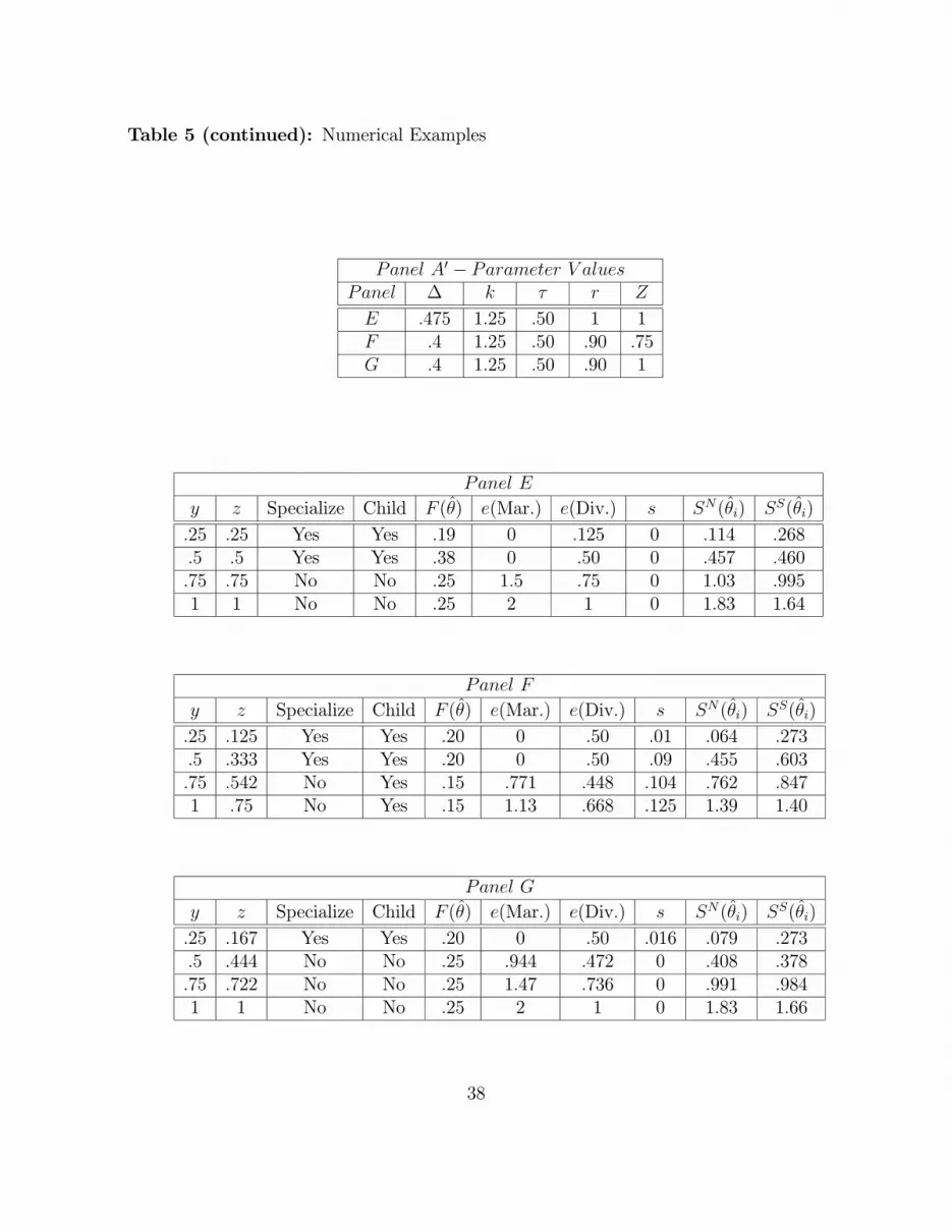
Table 5 (continued): Numerical Examples
Panel A0 − Parameter V aluesPanel ∆ k τ r Z
E .475 1.25 .50 1 1F .4 1.25 .50 .90 .75G .4 1.25 .50 .90 1
Panel E
y z Specialize Child F (θ̂) e(Mar.) e(Div.) s SN(θ̂i) SS(θ̂i)
.25 .25 Yes Yes .19 0 .125 0 .114 .268.5 .5 Yes Yes .38 0 .50 0 .457 .460.75 .75 No No .25 1.5 .75 0 1.03 .9951 1 No No .25 2 1 0 1.83 1.64
Panel F
y z Specialize Child F (θ̂) e(Mar.) e(Div.) s SN(θ̂i) SS(θ̂i)
.25 .125 Yes Yes .20 0 .50 .01 .064 .273.5 .333 Yes Yes .20 0 .50 .09 .455 .603.75 .542 No Yes .15 .771 .448 .104 .762 .8471 .75 No Yes .15 1.13 .668 .125 1.39 1.40
Panel G
y z Specialize Child F (θ̂) e(Mar.) e(Div.) s SN(θ̂i) SS(θ̂i)
.25 .167 Yes Yes .20 0 .50 .016 .079 .273.5 .444 No No .25 .944 .472 0 .408 .378.75 .722 No No .25 1.47 .736 0 .991 .9841 1 No No .25 2 1 0 1.83 1.66
38

Figure 1: The Proportion of College+ Educated by Sex (20-40 year olds)
39
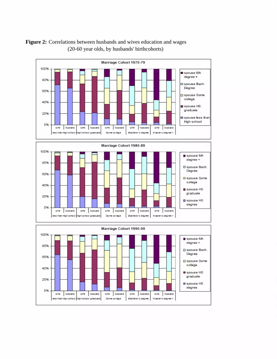
Figure 2: Correlations between husbands and wives education and wages (20-60 year olds, by husbands' birthcohorts)
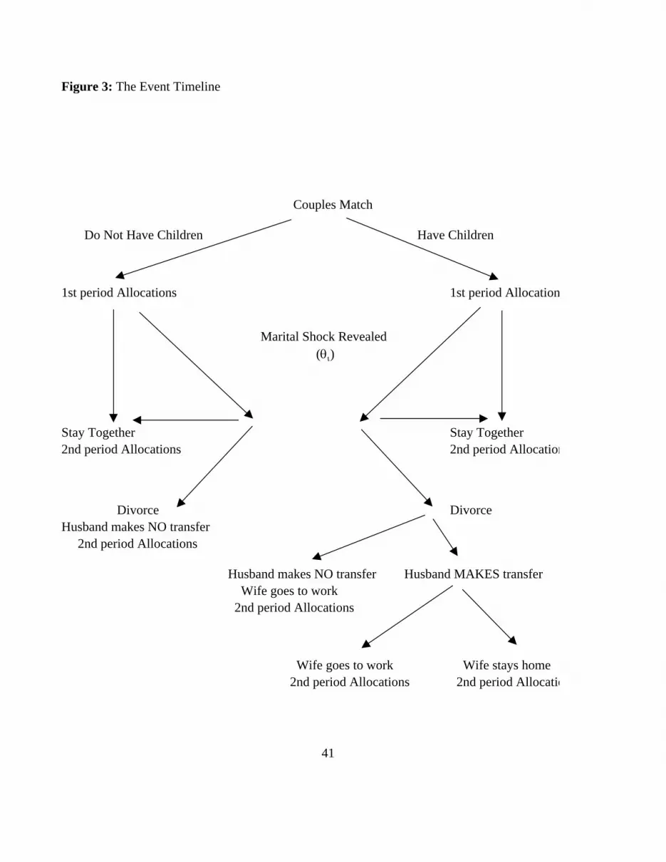
Figure 3: The Event Timeline
Couples Match
Do Not Have Children Have Children
1st period Allocations 1st period Allocation
Marital Shock Revealed (θι)
Stay Together Stay Together2nd period Allocations 2nd period Allocation
Divorce Divorce
Husband makes NO transfer 2nd period Allocations
Husband makes NO transfer Husband MAKES transfer Wife goes to work 2nd period Allocations
Wife goes to work Wife stays home 2nd period Allocations 2nd period Allocatio
41

Figure 4: Couples with kids, P(Divorce) = 0 z 1
Region A (δz > τ)
τ/δ
Region B
Region C
τ yFigure 5: Couples with kids, P(Divorce) = 1
z 1
Region A
τ/δ
Region B
Region D
Region C
τ y42
zzy τττ −−−= 2425
zzy τττ −−−= 244
Recommended


