Embed Size (px)
Citation preview

politecnico di milano
School of Civil, Environmental and Land ManagementEngineering
Department of Electronics, Information and Bioengineering
Master of Science in
Environmental and Land Planning Engineering
Effects of Climate Change onHydrology and HydropowerSystems in the Italian Alps
Supervisor:
prof . andrea castelletti
Assistant Supervisors:
dr . daniela anghileri
prof . paolo burlando
Master Graduation Thesis by:
pietro richelli
Student Id n. 799519
Academic Year 2013-2014


Nunc age, quo pacto pluvius concrescat in altisnubibus umor et in terras demissus ut imberdecidat, expediam. primum iam semina aquaimulta simul vincam consurgere nubibus ipsis
omnibus ex rebus pariterque ita crescere utrumqueet nubis et aquam, quae cumque in nubibus extat,
ut pariter nobis corpus cum sanguine crescit,sudor item atque umor qui cumque est denique membris.
Now come, and howthe rainy moisture thickens into being
in the lofty clouds, and how upon the lands’tis then discharged in down-pour of large showers,
I will unfold. And first triumphantlywill I persuade thee that up-rise together,
with clouds themselves, full many seeds of waterfrom out all things, and that they both increase-
both clouds and water which is in the clouds-in like proportion, as our frames increasein like proportion with our blood, as well
as sweat or any moisture in our members.
— Lucretius, De rerum natura, 55 B.C.E.translation by William Ellery Leonard


A C K N O W L E D G M E N T S
First and foremost, I would like to thank my supervisor, ProfessorAndrea Castelletti. With his lectures he aroused my interest in waterresources management and, with his valuable advices, he constantlyencouraged and supported my thesis.
I would sincerely like to thank Daniela Anghileri for her incessantsupport and commitment to get the most out of this research. Thanksto her I learnt a lot during the last few months.I would like to express my gratitude to Professor Paolo Burlando,who hosted me in Zurich at ETH, giving me the opportunity to workin an extremely stimulating and exciting environment.Moreover, I would like to thank the brilliant researches that, with theirhelp, contributed to this work: Matteo Giuliani, Simona Denaro, YuLi, and the entire research group in Hydrology and Water ResourcesManagement at ETH.I am also grateful to other master students that shared with me partof the thesis: Alessia, Slaven, and Beatrice.Besides the scientific aspects of the work, this thesis has been possi-ble also due to the help of a bunch of wonderful classmates. Manythanks go to Mattia, Iris, Davide, Umberto, Daniele, Simone, Rebecca,and Irene.
Academic support is a necessary but not sufficient condition to achievesuch a goal. In that sense I would like to thank my family for the un-conditional support and encouragement across these years of univer-sity. I owe to my father, my mother, and my sister a big slice of thisthesis. Moreover, special thanks go to my grandparents, who have al-ways been an example to me.
Finally, I need to thank Maya. Besides her huge effort in correctingand revising the text of the thesis, she stayed always close to me inthe past months with understanding, trust, and love.
And now, enjoy reading.
v


C O N T E N T S
Abstract xvRiassunto xvii1 introduction 1
1.1 Setting the Context 1
1.2 Objectives of the Thesis 2
1.3 Thesis Structure 3
2 methods and tools 5
2.1 Methodology 5
2.2 Models and Tools 6
2.2.1 Representative Concentration Pathways and IPCCAR5 6
2.2.2 General Circulation Models and Regional Cir-culation Models 10
2.2.3 The Quantile Mapping Statistical DownscalingTechnique 11
2.2.4 Topkapi-ETH 14
3 study site 17
3.1 Lake Como Territory 17
3.2 Hydropower Production 17
3.2.1 A2A 17
3.2.2 Enel 22
3.2.3 Edipower 27
3.2.4 Edison 30
3.2.5 Simplifications and Notes 30
4 climate change scenarios 33
4.1 The EURO-CORDEX Project 33
4.2 Selected Scenarios 34
4.3 Statistical Analysis of the EURO-CORDEX Scenarios 37
5 statistical downscaling 53
5.1 Historical Climate Observations 53
5.2 Statistical Downscaling via Quantile Mapping 53
5.3 Statistical Analysis of the Downscaled Scenarios 54
6 hydrological modelling 59
6.1 Topkapi-ETH Setup 59
6.1.1 Digital Elevation Model 59
6.1.2 Soil Map 60
6.1.3 Land Cover Map 60
6.1.4 Glacier Map 60
6.1.5 Thiessen Polygons for Temperature, Precipita-tion and Cloud Cover Transmissivity 60
6.1.6 Reservoirs 61
6.1.7 Groundwater Depth 61
vii

6.2 Calibration and Validation 66
6.3 Hydrological Scenarios Analysis 69
6.3.1 Experiment Setup 69
6.3.2 Impact of Climate Change on Streamflows 69
6.3.3 Impact of Climate Change on Glaciers 78
6.3.4 Impact of Climate Change on Reservoir Inflowsand Levels 81
7 uncertainty characterization 87
7.1 “Cascade of Uncertainty” in Climate Change ImpactStudies 87
7.1.1 Uncertainty in Radiative Forcing Modelling 90
7.1.2 Uncertainty in Global Climate Modelling 90
7.1.3 Uncertainty in Regional Climate Modelling 91
7.1.4 Uncertainty in Statistical Downscaling 91
7.1.5 Uncertainty in Hydrological Modelling 91
7.1.6 Uncertainty in Water Resources Management 92
7.2 Methods Used in the Literature to Address Uncertainty 92
7.3 Numerical Results 95
8 conclusions 107
Bibliography 111
a climate scenarios mash 119
b hydrological scenarios mash 139
viii

L I S T O F F I G U R E S
Figure 2.1 Thesis methodology 7
Figure 2.2 RCPs IPCC AR5 trajectories 9
Figure 2.3 GCMs 3D structure 10
Figure 2.4 RCM of the European domain 11
Figure 2.5 Bias correction with Quantile Mapping 13
Figure 2.6 Qq plot for Paris area, minimum temperature 13
Figure 2.7 Topkapi-ETH structure 14
Figure 3.1 Map of the Lake Como catchment 18
Figure 3.2 Map of the main reservoirs of the catchment 18
Figure 3.3 A2A hydropower network 19
Figure 3.4 Cancano reservoir 21
Figure 3.5 San Giacomo reservoir 21
Figure 3.6 Enel network in Valmalenco 23
Figure 3.7 Enel network in Val Gerola 23
Figure 3.8 Alpe Gera reservoir 24
Figure 3.9 Campo Moro reservoir 24
Figure 3.10 Inferno reservoir 25
Figure 3.11 Pescegallo reservoir 25
Figure 3.12 Trona reservoir 26
Figure 3.13 Edipower hydropower network 28
Figure 3.14 Montespluga reservoir 29
Figure 3.15 Truzzo reservoir 29
Figure 3.16 Edison hydropower network, Venina-Armisa link 30
Figure 3.17 Edison hydropower network, Ganda-Belviso link 31
Figure 3.18 Venina reservoir 31
Figure 3.19 Belviso reservoir 32
Figure 4.1 EUR-11 resolution over the area of interest 35
Figure 4.2 EUR-44 resolution over the area of interest 35
Figure 4.3 Boxplot climate control period 38
Figure 4.4 Boxplot climate RCP4.5 39
Figure 4.5 Boxplot climate RCP8.5 40
Figure 4.6 Cluster control period 41
Figure 4.7 Cluster RCP4.5 scenario 42
Figure 4.8 Cluster RCP8.5 scenario 42
Figure 4.9 RCA4/NCC temperature 44
Figure 4.10 RCA4/NCC precipitation 45
Figure 4.11 RCA4/NCC RR30 46
Figure 4.12 REMO/MPI temperature 48
Figure 4.13 REMO/MPI precipitation 49
Figure 4.14 RACMO/ICHEC temperature 50
Figure 4.15 RACMO/ICHEC precipitation 51
ix

Figure 5.1 Historical observation map 54
Figure 5.2 Chiavenna temperature quantile-quantile plot 55
Figure 5.3 RCP4.5 downscaled scenarios 56
Figure 5.4 RCP8.5 downscaled scenarios 56
Figure 5.5 Temperature downscaled scenarios 57
Figure 5.6 Precipitation downscaled scenarios 58
Figure 6.1 Digital Elevation Model 62
Figure 6.2 Soil type map 62
Figure 6.3 Land cover map 63
Figure 6.4 Glaciers depth 63
Figure 6.5 Temperature Thiessen polygons 64
Figure 6.6 Precipitation Thiessen polygons 64
Figure 6.7 Reservoirs 65
Figure 6.8 Groundwater depth 65
Figure 6.9 Fuentes location on the catchment 67
Figure 6.10 Calibration Fuentes 70
Figure 6.11 Boxplot streamflow Fuentes control period 71
Figure 6.12 Boxplot streamflow Fuentes RCP4.5 72
Figure 6.13 Boxplot streamflow Fuentes RCP8.5 72
Figure 6.14 Trajectories Fuentes control period 73
Figure 6.15 Trajectories Fuentes RCP4.5 73
Figure 6.16 Trajectories Fuentes RCP8.5 74
Figure 6.17 REMO/MPI Fuentes 76
Figure 6.18 RACMO/ICHEC Fuentes 77
Figure 6.19 Forni/Val Lia Glaciers Map 78
Figure 6.20 Glaciers discharge REMO/MPI 79
Figure 6.21 Glaciers discharge RACMO/ICHEC 80
Figure 6.22 REMO/MPI RCP4.5 A2A reservoir 82
Figure 6.23 REMO/MPI RCP8.5 A2A reservoir 83
Figure 6.24 RACMO/ICHEC RCP4.5 A2A reservoir 84
Figure 6.25 RACMO/ICHEC RCP8.5 A2A reservoir 85
Figure 7.1 Risk, uncertainty and ignorance scheme 88
Figure 7.2 The cascade of uncertainty 89
Figure 7.3 The cascade of uncertainty revised 89
Figure 7.4 GCM vs RCP uncertainty 97
Figure 7.5 RCM vs RCP uncertainty 98
Figure 7.6 GCM vs RCM uncertainty RCP4.5 98
Figure 7.7 GCM vs RCM uncertainty RCP8.5 99
Figure 7.8 Temperature Uncertainty 100
Figure 7.9 Precipitation Uncertainty 101
Figure 7.10 RCP-related uncertainty in hydrology I 102
Figure 7.11 RCP-related uncertainty in hydrology II 103
Figure 7.12 GCM-related uncertainty in hydrology 104
Figure 7.13 RCM-related uncertainty in hydrology 105
Figure A.1 RCA4/MIROC temperature 120
Figure A.2 RCA4/MIROC precipitation 121
x

Figure A.3 RCA4/NCC temperature 122
Figure A.4 RCA4/NCC precipitation 123
Figure A.5 RCA4/NOAA temperature 124
Figure A.6 RCA4/NOAA precipitation 125
Figure A.7 RCA4/CCC temperature 126
Figure A.8 RCA4/CCC precipitation 127
Figure A.9 RCA4/CNRM temperature 128
Figure A.10 RCA4/CNRM precipitation 129
Figure A.11 RCA4/ICHEC temperature 130
Figure A.12 RCA4/ICHEC precipitation 131
Figure A.13 HIRHAM/ICHEC temperature 132
Figure A.14 HIRAM/ICHEC precipitation 133
Figure A.15 CCLM/ICHEC temperature 134
Figure A.16 CCLM/ICHEC precipitation 135
Figure A.17 CCLM/MPI temperature 136
Figure A.18 CCLM/MPI precipitation 137
Figure B.1 RCA4/MIROC, Fuentes 140
Figure B.2 RCA4/NCC Fuentes 141
Figure B.3 RCA4/NOAA Fuentes 142
Figure B.4 RCA4/CCC Fuentes 143
Figure B.5 RCA4/CNRM Fuentes 144
Figure B.6 RCA4/ICHEC Fuentes 145
Figure B.7 HIRHAM/ICHEC Fuentes 146
Figure B.8 CCLM/ICHEC Fuentes 147
Figure B.9 CCLM/MPI Fuentes 148
L I S T O F TA B L E S
Table 2.1 RCPs characteristics 9
Table 3.1 Reservoirs characteristics 20
Table 4.1 EURO-CORDEX simulations characteristics 33
Table 4.2 Climate scenarios characteristics 34
Table 4.3 Combinations of EURO-CORDEX scenarios 36
Table 6.1 Calibration performance summary 69
A C R O N Y M S
RCM Regional Circulation Model
xi

GCM General Circulation Model
RCP Representative Concentration Pathway
IPCC Intergovernamental Panel for Climate Change
AR5 Fifth Assessment Report
GHGs Green House Gases
QM Quantile Mapping
SD Statistical Downscaling
ECP Extended Concentration Pathway
TE Topkapi-ETH
HWRM Hydrology and Water Resources Management
GC Grid Cell
IfU Institute of Environmental Engineering
IIASA International Institute for Applied System Analysis
NIES National Institute for Environmental Studies
JGCRI Joint Global Change Research Institute
SRES Special Report on Emission Scenarios
TAR Third Assessment Report
AR4 Fourth Assessment Report
DEM Digital Elevation Model
WRCP World Climate Research Program
CCT Cloud Cover Transmissivity
ARPA Regional Agency for the Protection of the Environment
MASH Moving Average over Shifting Horizon
NASA National Aeronautics and Space Administration
NGA National Geospatial-Intelligence Agency
USGS United States Geological Survey
DUSAF Destinazione d’Uso dei Suoli Agricoli e Forestali
GIS Geographical Information System
SRTM Shuttle Radar Topography Mission
xii

PPPs Policies, Plans, and Programs
ANOVA ANalysis Of VAriance
WMO World Meteorological Organization
xiii


A B S T R A C T
In this study we assess the impact of climate change on the hydro-logical cycle of an Alpine catchment and on the management of hy-dropower systems. We apply the traditional climate change impactstudy approach, known in the literature as “scenario-based” approach,to the case study of Lake Como catchment. The “scenario-based” ap-proach consists in employing a modelling chain, which comprises thedefinition of Green House Gases emission scenarios, the simulationof climate models and hydrological models, and the simulation of theimpact on water resources.We take into account an ensemble of climate scenarios, comprisingtwo Representative Concentration Pathways (RCPs), seven GeneralCirculation Models (GCMs) and five Regional Circulation Models(RCMs). The analysis of the climate scenarios on the domain of inter-est shows an increase in temperature and a seasonal shift in precip-itation, causing drier summers and more rainy winters. We apply astatistical downscaling to the climate scenarios in order to match theadequate spatial resolution needed for hydrological modelling. Weadopt Topkapi-ETH, a physically-based and fully distributed hydro-logical model, to reproduce the response of the catchment hydrologyto climate change. The employment of a spatially distributed modelis due to the possibility of assessing the impact of climate change ondifferent areas of the catchment. Moreover, Topkapi-ETH allows tosimulate anthropogenic infrastructures such as reservoirs and riverdiversions, which are widely present in the Lake Como catchment.The simulation results over the XXI century scenario show a seasonalshift in the hydrological cycle, with lower flow in summer, higherflow in winter, and an earlier snowmelt peak. This results in differentpatterns of storage building in the Alpine hydropower reservoirs.Finally, we analyze the uncertainty on hydro-climatic variables asso-ciated to climate modelling. Results show that the uncertainty relatedto the choice of the GCM is the most critical, but comparable to theone of the RCM. The choice of the RCP is generally less crucial forshort lead times, but it increases in relative terms for longer leadtimes.
xv


R I A S S U N T O
In questo studio viene valutato l’impatto del mutamento climatico sulciclo idrologico di un bacino alpino e sulla gestione di sistemi idroelet-trici. Il tradizionale approccio allo studio dell’impatto del mutamentoclimatico, noto in letteratura come “scenario-based”, viene applicatoad un caso di studio nelle Alpi italiane: il bacino idrografico del lagodi Como. L’approccio “scenario-based”, consiste nell’utilizzo di unacatena modellistica che include la definizione di scenari emissivi digas climalteranti, la simulazione di modelli climatici e idrologici e lasimulazione dell’impatto sulle risorse idriche.Viene preso in considerazione un ensemble di scenari climatici com-prendenti due Representative Concentration Pathway (RCP), setteGeneral Circulation Model (GCM) e cinque Regional Circulation Model(RCM). L’analisi degli scenari climatici sul dominio di interesse mostraun aumento delle temperature e uno shift stagionale delle precipi-tazioni, che prevede estati più siccitose ed inverni con maggiori pre-cipitazioni. Un downscaling statistico è applicato agli scenari climatici,per renderne la risoluzione spaziale adeguata alla modellazione idro-logica. Al fine di comprendere la risposta idrologica al mutamento cli-matico viene utilizzato Topkapi-ETH, un modello fisicamente basatoe spazialmente distribuito. L’utilizzo di un modello spazialmente dis-tribuito è dovuto alla possibilità di valutare l’impatto del cambia-mento climatico in diverse aree del bacino. Inoltre, Topkapi-ETH con-sente di implementare infrastrutture idrauliche, quali serbatoi idroelet-trici e canali di gronda, largamente presenti nel bacino. I risultatidella simulazione sull’orizzonte temporale del XXI secolo mostranouno shift stagionale nel ciclo idrologico, risultante in portate minorid’estate e maggiori in inverno, oltre che in una anticipazione del piccodi scioglimento nivale. Ciò comporta diverse traiettorie di invaso neiserbatoi idroelettrici.Infine, è analizzata l’incertezza sulle variabili idroclimatiche associatealla modellazione climatica. I risultati mostrano che l’incertezza legataalla scelta del GCM è la più critica, ma confrontabile con quella legataalla scelta del RCM. La scelta del RCP è generalmente meno crucialeall’inizio, ma cresce con il passare del tempo lungo l’orizzonte tem-porale.
xvii

1I N T R O D U C T I O N
1.1 setting the context
Climate change is considered to be a key factor in the availabilityof water resources during the XXI century [IPCC, 2014]. The rise oftemperature and the shift in the distribution of precipitation at theglobal scale will affect the hydrological cycle and thus the water re-lated human activities. The hydrology of the Alpine regions is likelyto be affected more then others since they are characterized by a highpresence of snow and glaciers and are more sensitive to climate con-ditions [Zierl and Bugmann, 2005; Beniston, 2003]. The temperatureincrease will cause an earlier snowmelt and a shift in temporal andspatial precipitation patterns will considerably change water avail-ability. Furthermore, the impact of climate change on hydrology willbe accentuated by the glaciers retreat [Haeberli and Beniston, 1998].The hydropower plants installed in the Alps play a key role in the sup-ply of electricity and, due to their flexibility compared to other elec-tricity sources, they also provide a certain stability in the internationalnetwork [Gaudard et al., 2014]. Moreover, their importance as a keyresource is growing with the increase of power installed in intermit-tent renewable energy sources such as wind and solar power. Sincethe patterns of production of wind and solar power are very irreg-ular, and other traditional sources of electricity (e.g., nuclear powerand fossil fuel) are less flexible, hydropower is a strategic source forthe future. Hydropower in a mountainous country like Switzerlandrepresents 59.7% of electricity generation [Energiebundesamt, 2012],while in Italy this value decreases to 13.2% [Terna, 2012], mantaininganyhow a considerable share of the national production. The changescurrently taking place in the electricity market due to the increasingshare of renewable energies and the implementation of an energystock exchange are leading to several transformations in which hy-dropower will be one of the main players.In such a context, it is important to investigate the complex relation-ship occurring among climate, water availability, and hydropowerproduction.When dealing with climate change, the uncertainty related to futureprojection can not be neglected. Climate change impact studies arethe result of a complex modelling chain, which comprises the defi-nition of the Representative Concentration Pathway (RCP), the Gen-eral Circulation Model (GCM), Regional Circulation Model (RCM), thedownscaling procedure, the hydrological modelling, and the mod-
1

2 introduction
elling of the reservoirs. In recent years considerable effort has beenspent in order to characterize the uncertainty related to climate andhydrology. Since an uncertainty analysis can be addressed in severaldifferent ways, a large number of approaches have been proposed inthe past years, to tackle specific aspects of the problem. For example,Murphy et al. [2004] analyzed the changes in the probability densityfunctions of some climate indicators, with a probabilistic approach.Hawkins and Sutton [2009] tried instead to quantify how the differentsources of uncertainty change with the lead time of the projection. An-other approach was proposed by Finger et al. [2012] that attempted,through an analysis of the variance, to quantify how different sourcesof uncertainty affect the climate during the twelve months of the year.
1.2 objectives of the thesis
The main objective of this thesis is to assess the impact of climatechange on hydrology and hydropower production in the Italian Alps.In particular, we focus on the Lake Como catchment. We adopt theclassical workflow of climate change impact studies, known in theliterature as “scenario-based”. The first step is the analysis of climatechange scenarios. More precisely, we consider temperature and pre-cipitation as projected by an ensemble of climate models forced withtwo different Representative Concentration Pathways RCPs (4.5 and8.5). These scenarios refer to the EURO-CORDEX project and theIntergovernamental Panel for Climate Change (IPCC) Fifth Assess-ment Report (AR5). The next step is to apply a statistical downscal-ing, since the spatial resolution of the climate scenarios is not fineenough for the hydrological modelling. Then, a fully distributed andphysically-based hydrological model is calibrated and simulated. Theimportance of employing a spatially distributed hydrological modelis related to the possibility of assessing the response of hydrology toclimate change in every single part of the catchment, allowing spa-tial analyses on river network, glaciers, and reservoirs. The last stepcomprises the assessment of the impact of hydrological scenarios onthe management of the reservoirs that can, thanks to the spatially dis-tributed hydrological modelling, be jointly taken into account. Alongwith this workflow, an uncertainty characterization is carried out inorder to assess the contribution of the single modelling componentsto the global uncertainty.Ultimately, the main innovative contributions of this thesis are thefollowing:
• The analysis of the predicted impact of climate change on theSouthern Alps and on the Lake Como catchment, within theEURO-CORDEX framework.

1.3 thesis structure 3
• The employment of a fully distributed hydrological model, inorder to analyze the complexity of the response of hydrologyto climate change, together with the impact on the reservoirsmanagement.
• The uncertainty characterization, carried out in order to assess,within the “scenario-based” workflow, where most of the uncer-tainty is located.
1.3 thesis structure
This thesis is structured in the following parts:
• The next chapter (2) contains a description of the methods andtools used in the thesis: the climate models, the statistical down-scaling technique and the hydrological model.
• Chapter 3 provides a comprehensive description of the studyarea of the Lake Como catchment.
• Chapter 4 is about the impact of climate change on the studysite. The IPCC AR5 is introduced and the EURO-CORDEX projectwith its climate models is described. Then the results of ouranalysis on the climate change are shown.
• Chapter 5 is intended to describe the adopted downscaling pro-cedure, starting with the datasets used and concluding withsome comparisons between historical observations and down-scaled climate scenarios.
• Chapter 6 describes the application of the hydrological modelTopkapi-ETH to the Lake Como catchment. At the beginning acomprehensive description of the model properties and inputdata for setup and calibration is given to the reader. In the sec-ond part the hydrological scenarios obtained via simulation ofTopkapi-ETH on the case study are analyzed.
• Chapter 7 tackles the issues related to uncertainty. It is shownhow the problem has been approached in the past and whichprocedure is adopted in this work to give a quantitative de-scription of the single modelling component contribution to theglobal uncertainty.


2M E T H O D S A N D T O O L S
2.1 methodology
The general framework used in this thesis to assess the impact ofclimate change is usually addressed in literature as "top-down" or"scenario-based" approach [Wilby and Dessai, 2010]. This approachconsists on the application of a cascade of models, from the demo-graphic development to the management of a water system. Gener-ally, in the field of water resources management this modelling cas-cade includes:
• The definition of a Green House Gases (GHGs) emission sce-nario.
• The global climate modelling via General Circulation Models(GCMs).
• The regional climate modelling via Regional Circulation Models(RCMs).
• The application of statistical downscaling in order to possiblyrefine even more the resolution of the climate variables.
• The employment of a hydrological model, to evaluate the stream-flow scenarios.
• The modelling of the impact on water resources management.
Another possible way to approach climate change impact studies isthe so-called "bottom-up" or "vulnerability-based" approach [Wilbyand Dessai, 2010]. In this different approach the perspective is re-versed since it relies mainly on the observation of the current watersystem and less on the future scenarios. It usually implies the twofollowing main steps:
• The identification of the current water system vulnerabilities.
• The definition of better strategies to deal with them.
The integration of the two methods is probably the best way to set acomprehensive analysis and approach policy design in climate changeconditions. Nevertheless, as the main goal of this thesis is to assessthe impact of the climate change on existing hydropower reservoirs,the first approach ("scenario-based") is applied. The models and toolsapplied to the Lake Como catchment to implement the workflow of
5

6 methods and tools
the scenario-based approach are graphically shown in Figure 2.1 andlisted here:
• We consider two Representative Concentration Pathways in theframework of IPCC Fifth Assessment Report, they are RCP4.5 andRCP8.5.
• We take into account an ensemble of combinations of GCMs andRCMs to evaluate the effect of climate change on the variables oftemperature and precipitation on the Lake Como catchment.
• As the resolution of RCMs is still to coarse for a physically-basedhydrological model we apply a statistical downscaling using theQuantile Mapping technique.
• We calibrate a fully distributed and physically-based hydrologi-cal model (Topkapi-ETH) on the catchment and simulate it, fedby the downscaled scenarios, in order to assess the impact ofclimate change on the hydrology.
• Within Topkapi-ETH we apply an operative rule to the reser-voirs in the catchment, to evaluate how changes in hydrologywill reflect on the reservoirs.
2.2 models and tools
In the next sections we describe the models and tools used in the the-sis, namely the RCPs, the GCMs and RCMs, the statistical downscalingtechnique and the hydrological model.
2.2.1 Representative Concentration Pathways and IPCC AR5
The Representative Concentration Pathways are Green House Gases(GHGs) concentration trajectories adopted by the IPCC for its AR5 in2014. They describe possible climate futures on the basis of the radia-tive forcing values (changes in balance between incoming and outgo-ing radiation to the atmosphere, caused by its composition) relative tothe pre-industrial period. RCPs substitute the Special Report on Emis-sion Scenarios (SRES) projections published in 2000, and used in IPCC
Third Assessment Report (TAR) e Fourth Assessment Report (AR4).The SRES describes emission scenarios. Emission scenarios are a repre-sentation of the future discharges in the atmosphere of GHGs that pro-vide input to climate models. To be produced they require assump-tions about patterns of economic and demographic growth, technol-ogy development and future energy consumption. The SRES are com-plemented by socio-economic storylines, which help in their interpre-tation. Although they have been widely used, after over a decade of

2.2 models and tools 7
Figure 2.1: Flow chart of the main steps followed in the analysis. On theleft side of the graph, are shown the traditional steps of ascenario-based workflow in water resources management. Onthe right side are listed the sources of the tools used in eachspecific step: the RCPs were considered in the framework ofthe IPCC AR5; the climate scenarios were retrieved from theEURO-CORDEX project; the downscaling technique used wasthe Quantile Mapping; the hydrological model employed wasTopkapi-ETH, which comprises reservoir operative rules.

8 methods and tools
climate change studies, new economic data and technology develop-ments, different and new scenarios were released [Moss et al., 2010].The new scenarios, rather than using storylines, use radiative forc-ing trajectories, which are not associated with unique socio-economicscenarios, but can result from many combinations of demographic,economic and technology futures. Since climate models require dataon concentrations of radiatively active constituents in the atmosphere,the research community identified a specific emission scenario aspathway towards achieving each radiative forcing trajectory. This stepwas necessary to make them usable in climate modelling and com-pare them with the old SRES scenarios. A selection process took placein order to identify the final RCPs, with criteria established by the re-search community. The main criteria adopted were: the compatibilitywith the complete range of emission scenarios existing in literature; amanageable and even number of scenarios (in order to avoid a centralone to be taken as ‘best estimate’); a clear separation of the radiativeforcing trajectories on the long term, to make them distinguishable.The IPCC Working Group III used these criteria in 2007, in order toidentify first 32 potential candidates and then to make the final choiceon four of them. Figure 2.2 illustrates the final chosen RCPs amongthe other candidates. The four RCPs selected in the IPCC AR5 (RCP2.6,RCP4.5, RCP6, RCP8.5) are named after the range of radiative forcingvalues at the end of the century (2100) relative to pre-industrial val-ues (+2.6, +4.5, +6.0 and +8.5 W/m2). The main characteristics of eachscenario (summarized in Table 2.1) are the following:
• RCP2.6 was developed in the Netherlands by the IMAGE mod-elling team. The emission path is representative of scenarios inliterature that lead to very low GHGs levels, It is also know as the“peak-and-decline scenario”, reaching a maximum of radiativeforcing around mid-century (+3.1 W/m2) and then declining[van Vuuren et al., 2007].
• RCP4.5 was developed in the United States by the Joint GlobalChange Research Institute (JGCRI). It is a stabilization scenarioin which the total radiative forcing is stabilized, without over-shoot (without reaching a peak), shortly after 2100 [Clarke, 2007;Smith and Wigley 2006].
• RCP6.0 was developed in Japan at the National Institute for Envi-ronmental Studies (NIES). It is again a stabilization scenario thatpredicts that the total radiative forcing will stabilize, withoutovershoot, shortly after 2100 thanks to the application of sometechnologies and strategies to reduce GHGs emissions. The sta-bilization of radiative forcing will take place like in RCP4.5, butwith a higher value of GHGs concentration [Fujino, 2006; Hijiokaet al. 2008].

2.2 models and tools 9
Figure 2.2: RCPs trajectories (in bold) compared to the ones of other candi-tates, taken from Moss et al. [2010]
• RCP8.5 was developed in Austria at the International Institutefor Applied System Analysis (IIASA) using MESSAGE-MACRO,a model that incorporates energy supply with a non-linear macroe-conomic model. This RCP presents increasing GHGs emissionsover time and is representative of scenarios in literature thatshow high GHGs concentrations [Riahi et al., 2007].
Another interesting new feature of the RCPs, with regarding to theSRES, is that there was an attempt to go beyond 2100 with the projec-tions. The Extended Concentration Pathway (ECP)s were developedextending GHGs concentrations and emissions time series. The ECPs
radiative co2 temperature sres
name forcing (ppm)anomaly (°c) pathway equivalent
RCP8.5 8.5 W/m21370 4.9 Rising A1F1
RCP6.0 6.0 W/m2850 3.0 Stabilization B2
RCP4.5 4.5 W/m2650 2.4 Stabilization B1
RCP6.0 2.6 W/m2490 1.5 Peak and Decline None
Table 2.1: IPCC AR5 RCPs main characteristics
10 methods and tools
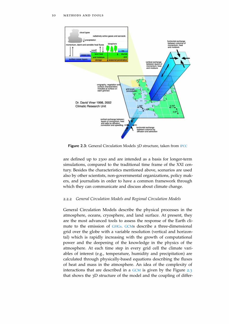
Figure 2.3: General Circulation Models 3D structure, taken from IPCC
are defined up to 2300 and are intended as a basis for longer-termsimulations, compared to the traditional time frame of the XXI cen-tury. Besides the characteristics mentioned above, scenarios are usedalso by other scientists, non-governmental organizations, policy mak-ers, and journalists in order to have a common framework throughwhich they can communicate and discuss about climate change.
2.2.2 General Circulation Models and Regional Circulation Models
General Circulation Models describe the physical processes in theatmosphere, oceans, cryosphere, and land surface. At present, theyare the most advanced tools to assess the response of the Earth cli-mate to the emission of GHGs. GCMs describe a three-dimensionalgrid over the globe with a variable resolution (vertical and horizon-tal) which is rapidly increasing with the growth of computationalpower and the deepening of the knowledge in the physics of theatmosphere. At each time step in every grid cell the climate vari-ables of interest (e.g., temperature, humidity and precipitation) arecalculated through physically-based equations describing the fluxesof heat and mass in the atmosphere. An idea of the complexity ofinteractions that are described in a GCM is given by the Figure 2.3that shows the 3D structure of the model and the coupling of differ-

2.2 models and tools 11
Figure 2.4: Example of RCM over the European domain, taken from WMO
ent components of the climate such as land, atmosphere, oceans andice-sheets. Even though the resolution of GCMs has improved in thepast years, it is still not fine enough to provide the accuracy neededfor climate change impact studies. Further refinement of GCMs’ out-puts can be obtained by applying some downscaling techniques. Thedynamical downscaling technique consists in nesting a Regional Cir-culation Model into a GCM. RCMs have the same structure of GCMsbut work at a finer spatial resolution so account for more details,such as orography, land use and small-scale atmospheric features.They provide better accuracy needed in climate change impact stud-ies with a resolution that is generally between 10 km and 50 km(Figure 2.4). The nesting procedure consists in the GCMs providingthe boundary conditions for the RCM run. The dynamical downscal-ing is particularly attractive for mountainous [Frei et al., 2006] andcoastal area, where the coarse spatial resolution of a GCM cannot de-scribe correctly the physical processes taking place, which are usuallydominated by local circulation phenomena, rather than global. Eventhough the reduced domain area could increase the speed of the sim-ulation, the finer resolution makes RCMs extremely computationallyintensive [Fowler and Tebaldi, 2007].
2.2.3 The Quantile Mapping Statistical Downscaling Technique
In the majority of climate change impact studies the resolution ofGCMs and RCMs is not fine enough and computational limits do notallow further dynamical downscaling. In those cases the mismatchbetween global climate and local scale can be tackled with StatisticalDownscaling (SD) techniques. SD is based on the fact that local cli-mate is influenced by two main factors: the large-scale climate andthe small-scale local features (e.g., land cover, topographic features,coasts [Von Storch, 1995]). Local climate variables are derived first de-termining a statistical relationship, which links the large-scale pre-dictor to the small-scale predictand. For this part of the work, his-

12 methods and tools
torical observations of the local climate are required. After that, theestimated statistical relationship between predictor and predictand isapplied to the output of the climate model, in order to obtain the localclimate data [Wilby et al., 2004]. Usually predictors and predictandsrepresent the same physical variable, but it is not strictly necessary.The SD methods are often used in climate change impact studies asthey are computationally inexpensive, especially compared to dynam-ical downscaling techniques. Other advantages are that they can pro-vide site-specific information, as points, typically needed in climatechange impact studies [Mearns et al., 2003] and the removal of themodel bias [Boe et al., 2007]. A limit is that they strongly depend onthe quality of the historical observations, thus they can be used onlywhen reliable datasets are available. Another weakness of SD methodsin climate change impact studies is that they assume that the relation-ship between the two variables will remain the same in the future un-der different climate forcing which might not be true under climatechange conditions. Several SD methods have been proposed, amongwhich the most common are: delta change method [Hay et al., 2000],neural network [Olsson et al., 2001], analog method [Zorita, 1999], weathergenerator [Wilks and Wilby, 1999], unbiasing method [Deque, 2007]and quantile mapping [Boe et al., 2007]. In this study Quantile Map-ping (QM) has been adopted, due to its simplicity and flexibility. TheQM consists of generating a correction function (f) between the cli-mate model outputs distribution and the observations distributionand its application to remove the bias. An example of bias removalis shown if Figure 2.5 [Boe et al., 2007]. As input the QM requires thehistorical observations, the model outputs of a control run during thesame period and the forecast model outputs over the future scenario.The procedure consists in two main phases:
• CALIBRATION PHASE: the correction function (f) between thecumulative density function (cdf) of the model outputs in thecontrol run (C) and the cdf of the observations (O) is calibrated.An example is shown in Figure 2.6, for the minimum tempera-ture in the Paris area [Deque, 2007].
O = f ′(C)
• PROJECTION PHASE: the calibrated correction function (f ′) isand applied to the variables from the forecast (F), removing thebias. A linear interpolation is applied between two percentiles.The result of the operation is the downscaled time series (F ′).
F ′ = f ′(F)
In the QM algorithm used in this work, if a forecast value exceedsthe quantiles computed (which might happen under climate changeconditions) a constant correction equal to the 99
th or 1st quantile
is applied. The calibration phase can be done yearly, seasonally ormonthly, as the model error might differ during the year.

2.2 models and tools 13
Figure 2.5: Scheme of bias correction using Quantile Mapping. cdf standsfor Cumulative Distribution Function. The subscript o, f, c standfor the historical observation, the climate scenario model out-put and the control simulation respectively. For the value xf(d)of the variable x in the day d in the climate scenario, thecorresponding seasonal cumulative frequency Pc(xf(d)) whereP(x) = Pr(X 6 x) is searched in the calculated cdf of theclimate control simulation. After that, the value of x such asPo(x) = Pc(xf(d)) is searched on the cdf of the historical ob-servations. This final value (xfcorr(d)), is used as the correctedvalue of xf(d) [Boe et al., 2007].
Figure 2.6: Quantile–quantile plot for model outputs (x-axis) versus histor-ical observations (y-axis) of the minimum temperature (°C) inthe Paris area during the period 1961-1990. Solid line representswinter values, while dash line summer values [Deque, 2007].

14 methods and tools
Figure 2.7: Topkapi-ETH Structure. The arrows represent the flows takingplace in a grid cell.
2.2.4 Topkapi-ETH
When dealing with climate change, it is very important to correctlydescribe the physical processes occurring in the hydrological cycle, inorder to assess how changes in climate affect the hydrological regimes.Therefore, it is highly preferable to employ physically-based model,rather than empirical and conceptual ones. The model adopted inthis thesis is Topkapi-ETH (Topographic Kinematic Approximationand Integration model), originally developed by Todini and others[Ciarapica and E., 2002; Liu and Todini, 2002; Liu and Todini, 2006].After some enhancements at the department of Hydrology and WaterResources Management (HWRM), in the Institute of EnvironmentalEngineering (IfU) of the Federal Institute of Technology in Zurich, ittook the current name, Topkapi-ETH (TE).Topkapi-ETH presents a regular grid in which the smallest computa-tional element is the single Grid Cell (GC). Flow directions are definedas shown in Figure 2.7 with a single outflow direction (one down-stream GC) and up to three upstream cells. The model uses a verticaldiscretization of belowground in three layers. The deepest layer mim-ics the behavior of slow components such as fractured or porous rockacquifers, while the first two layers represents deep and shallow soilas non-linear reservoir. GCs are connected to the surface and subsur-face according to topographic gradients. The potential infiltration rateis calculated with an empirical formula and runoff can result fromsaturation excess or infiltration processes. The topographic effects on

2.2 models and tools 15
radiation (particularly significant in mountainous terrains) are regu-lated as described in Corripio [2003]. The evapotraspiration is regu-lated by the Priestly Taylor equation [Priestley and Taylor, 1972] anda monthly correction is applied to distinguish between different landuses. Snow and ice-melt are calculated with an empirical temperatureindex model, which is fed only by shortwave radiation and air tem-perature [Pellicciotti et al., 2005; Carenzo et al., 2009]. Topkapi-ETHcompared to other physically-based state-of-art hydrological modelsdoes not represent the rigorousness and richness of hydrological pro-cesses [Fatichi et al., 2013], but it is a reasonable trade-off between hy-drological representation and computational time for large catchmentconsidering also the long time horizons and the large number of sim-ulation required by the different climate change scenarios consideredin this analysis. Moreover the latest upgrade of the model, done byHWRM at ETH Zurich gives the possibility to take into account someanthropogenic infrastructures such as reservoirs, river diversions andwater abstractions. The reservoirs are described by their technical fea-tures such as maximum outflow, spillway definition, volume-levelcurves, and environmental flows and some simple operational rulesare implemented. Other artificial facilities such as diversion channelsand water abstractions can be included in the model setup.In Topkapi-ETH, the values of air temperature, cloud cover trasmis-sivity and precipitation for each GC at the temporal and spatial resolu-tion selected for the model simulation are the meteorological inputsrequired. Furthermore, Topkapi-ETH requires a series of spatial in-puts for the model setup: a digital elevation map of the catchment,a soil map, a land use map, and a map of the glaciers. For the gridcells time series the available outputs are: water volume in upper sub-surface layer, effective saturation in upper subsurface layer, effectivesaturation in lower subsurface layer, effective saturation in ground-water aquifer, channel flow, flow in upper subsurface layer, flow inlower subsurface layer, flow in groundwater aquifer, and snow waterequivalent.


3S T U D Y S I T E
3.1 lake como territory
The Lake Como, also known with its traditional Latin name “Lario”is a natural lake with glacial origins (Figure 3.1). With its 140 me-ters of depth is the fifth deepest European lake (after four Norwegianlakes) and with its 145 km2 of surface it is the third largest Italianlake after Lake Garda and Lake Maggiore. The lake is surroundedby mountains and receives water by 37 tributaries (Mera and Addabeing the main ones). The River Adda, the only emissary of the lake,flows through the Lombardy territory until it reaches the River Po.The Lake Como is regulated by the Olginate dam, located near Lecco.The catchment of River Adda, closed at the Olginate dam, has anarea of 4762 km2 of which 90% is Italian and the remaining 10% isSwiss. The Swiss part of the basin is composed by the territory of ValBregaglia and Val Poschiavo. The River Spoel, which naturally flowsinto the Danube catchment, is partly diverted into the Lake of SanGiacomo. At the bottom of the Valtellina, the River Adda flows atFuentes into the Lake Como, with an average discharge of 88m3/s[Giacomelli et al., 2008]. A snowmelt peak in late spring and a sec-ondary peak in autumn characterize the hydrological year, while inwinter average streamflows are considerably lower.
3.2 hydropower production
Since the beginning of the past century the area upstream the LakeComo has been exploited with the construction of many dams andartificial lakes. Today it is a complex hydropower system, with severalbig reservoirs, run by four main energy companies: A2A, Enel, Edisonand Edipower. Figure 3.2 shows the location of the main reservoirs,while Table 3.1 illustrates their main characteristics.
3.2.1 A2A
A2A (previously named AEM, Azienda Elettrica Milanese) owns awidespread and extensive hydraulic network in Valtellina (Figure 3.3).The two main artificial lakes are Cancano and San Giacomo (Figures3.4 and 3.5), which feed a dense network of power plants headedby the main one of Premadio. They are two contiguous reservoirs,located in the municipality of Valdidentro, in the Fraele Valley. Thefirst lake, San Giacomo was built in 1950, has an altitude measured
17

18 study site
Figure 3.1: Map of the Lake Como catchment. It is possible to distinguishthe four main sub-catchments: the River Adda, the River Mera,the catchment of the Lake Como and the catchment of the Spoel,which naturally would be a tributary of the Danube, but it isartificially diverted to the Cancano reservoir.
Figure 3.2: Map of the main reservoirs of the catchment. It is possible to seehow some reservoirs where conceptually merged together forthe analysis: Cancano and San Giacomo, Alpe Gera and CampoMoro and Trona, Inferno and Pescegallo.

3.2 hydropower production 19
Figure 3.3: A2A hydropower network in Valtellina, adapted from A2A

20 study site
natural connected dam
name storage basin basin altitude company
Mm3 Km2 Km2 m a.s.l
San Giacomo 64.0 18.7 322.3 1952 A2A
Cancano 124.0 36.0 322.3 1902 A2A
Alpe Gera 68.1 39.9 50.9 2128 Enel
Campo Moro 10.8 39.9 50.9 1969 Enel
Inferno 4.2 1.1 0.3 2088 Enel
Trona 5.4 2.6 11.5 1805 Enel
Pescegallo 1.1 0.9 1.0 1863 Enel
Montespluga 32.6 24.0 2.9 1904 Edipower
Truzzo 20.0 10.0 5.5 2088 Edipower
Venina 11.2 8.3 11.8 1824 Edison
Belviso 50.1 27.3 20.1 1486 Edison
Table 3.1: Characteristics of the main reservoirs existing in Valtellina andValchiavenna
at the top of its dam of 1951.5 m and a maximum storage of 64 Mm3.It is fed by the channel Spoel and the streams Gravia, Frodolfo, Alpe,Zebrù, Forcola, and Braulio together with the River Adda. The LakeCancano, located directly next to San Giacomo, has a capacity of 124
Mm3 and a dam, built in 1956, located at 1902 m a.s.l.. The reservoiris fed directly by Lake San Giacomo and the channel Viola. The en-tire catchment has an area of 36 Km2, but considering the connectedbasin it goes up to 322.3 Km2. The power plant of Premadio, locateddownstream the two big reservoirs, has a total installed capacity of226 MW, thanks to six Pelton turbines. The maximum streamflow inthe power plant is 39 m3/s.

3.2 hydropower production 21
Figure 3.4: Cancano reservoir, source: ARPA Lombardia
Figure 3.5: San Giacomo reservoir, source: ARPA Lombardia
22 study site
3.2.2 Enel
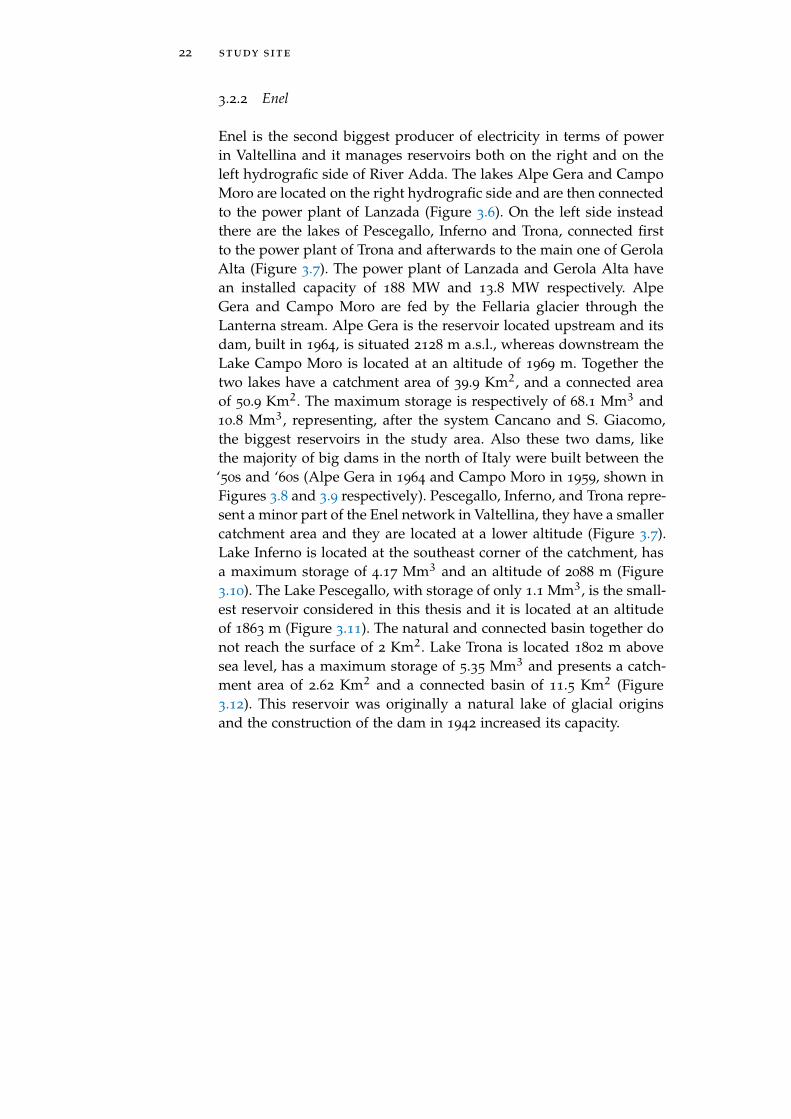
Enel is the second biggest producer of electricity in terms of powerin Valtellina and it manages reservoirs both on the right and on theleft hydrografic side of River Adda. The lakes Alpe Gera and CampoMoro are located on the right hydrografic side and are then connectedto the power plant of Lanzada (Figure 3.6). On the left side insteadthere are the lakes of Pescegallo, Inferno and Trona, connected firstto the power plant of Trona and afterwards to the main one of GerolaAlta (Figure 3.7). The power plant of Lanzada and Gerola Alta havean installed capacity of 188 MW and 13.8 MW respectively. AlpeGera and Campo Moro are fed by the Fellaria glacier through theLanterna stream. Alpe Gera is the reservoir located upstream and itsdam, built in 1964, is situated 2128 m a.s.l., whereas downstream theLake Campo Moro is located at an altitude of 1969 m. Together thetwo lakes have a catchment area of 39.9 Km2, and a connected areaof 50.9 Km2. The maximum storage is respectively of 68.1 Mm3 and10.8 Mm3, representing, after the system Cancano and S. Giacomo,the biggest reservoirs in the study area. Also these two dams, likethe majority of big dams in the north of Italy were built between the‘50s and ‘60s (Alpe Gera in 1964 and Campo Moro in 1959, shown inFigures 3.8 and 3.9 respectively). Pescegallo, Inferno, and Trona repre-sent a minor part of the Enel network in Valtellina, they have a smallercatchment area and they are located at a lower altitude (Figure 3.7).Lake Inferno is located at the southeast corner of the catchment, hasa maximum storage of 4.17 Mm3 and an altitude of 2088 m (Figure3.10). The Lake Pescegallo, with storage of only 1.1 Mm3, is the small-est reservoir considered in this thesis and it is located at an altitudeof 1863 m (Figure 3.11). The natural and connected basin together donot reach the surface of 2 Km2. Lake Trona is located 1802 m abovesea level, has a maximum storage of 5.35 Mm3 and presents a catch-ment area of 2.62 Km2 and a connected basin of 11.5 Km2 (Figure3.12). This reservoir was originally a natural lake of glacial originsand the construction of the dam in 1942 increased its capacity.

3.2 hydropower production 23
Figure 3.6: Enel network in Valmalenco, where the dams of Campo Moroand Alpe Gera are located, source: Enel
Figure 3.7: Enel network in Val Gerola, where the dams of Trona and In-ferno and Pescegallo are located, source: Enel

24 study site
Figure 3.8: Alpe Gera reservoir, source: ARPA Lombardia
Figure 3.9: Campo Moro reservoir, source: ARPA Lombardia

3.2 hydropower production 25
Figure 3.10: Inferno reservoir, source: ARPA Lombardia
Figure 3.11: Pescegallo reservoir, source: ARPA Lombardia

26 study site
Figure 3.12: Trona reservoir, source: ARPA Lombardia

3.2 hydropower production 27
3.2.3 Edipower
The reservoirs belonging to Edipower are located in Valchiavenna,along the rivers Liro and Mera (Figure 3.13). River Mera’s source islocated over 2800 m above the sea level in Switzerland and it reachesthe Italian territory in Castesegna. Liro’s source is located near theSpluga pass and after roughly 25 Km it flows into the Mera near thetown of Chiavenna. Due to particular climatic conditions this arealocated north of the Lake Como is characterized by humid windsand frequent and intense precipitation events. Downstream the tworeservoirs, it is built a dense hydropower network, whose biggestplant is the one of Mese, having an installed capacity of 170 MW.Lake Montespluga is located between the Spluga pass and Madesimo,it has a maximum storage of 32.6 Mm3 and an altidude of 1903.5 m.It is closed by two dams, Cardanello and Stuetta, both built in 1932
and it has a catchment area of 24 Km2 and a connected basin if 2.85
Km2 (Figure 3.14). Lake Truzzo is located in a valley perpendicularto Valchiavenna (Valle del Drogo) and has a maximum storage of 20
Mm3. After the one of the Alpe Gera, it is the highest among the onesconsidered in this analysis (2088 m a.s.l.). It has a catchment area of10 Km2 and a connected basin of 5.5 Km2 (Figure 3.15).

28 study site
Figure 3.13: Edipower hydropower network in Valchiavenna, source:Edipower

3.2 hydropower production 29
Figure 3.14: Montespluga reservoir, source: ARPA Lombardia
Figure 3.15: Truzzo reservoir, source: ARPA Lombardia

30 study site
Figure 3.16: Edison hydropower network in the area of the Lake Venina,source: Edison
3.2.4 Edison
The facilities of Edison in the area of Valtellina were built by Falcksteelworks between the ‘20s and the ‘60s and they consist of twohydraulic links: the link Venina-Armisa (Figure 3.16) and the linkGanda-Belviso (Figure 3.17). Lake Venina is fed mainly by the homony-mous river and it is closed downstream by a dam located 1824 mabove the sea level. It has a maximum storage of 11.2 Mm3 and anatural catchment area of 8.3 Km2, while the connected basin is 11.8Km2 wide. Lake Venina feeds the homonymous plant, which has atotal capacity of 67 MW (Figure 3.18). Lake Belviso owes its name tothe River Belviso by which it is fed and it was born with the con-struction of the Frera dam (1486 m a.s.l). Due to the strategic locationnext to several valleys it has a catchment area of 27.3 Km2 and 20.1Km2 of connected basin. With a maximum storage of 50.1 Mm3, LakeBelviso is the fourth biggest lake among the ones described here (Fig-ure 3.19). Lake Belviso feeds with its water the two main plants of thelink: Ganda and Belviso, which have both a capacity of 66 MW and astreamflow concession of 14 m3/s.
3.2.5 Simplifications and Notes
As already mentioned, not the whole river catchment of Adda is inthe Italian territory. The part of the catchment in the Helvetic territoryis anyhow exploited with hydropower reservoirs and plants, but inthis analysis we have to exclude the Swiss reservoirs due the scarcityof data that would mislead the analysis. These excluded lakes are:Lake White, Lake Poschiavo, Lake Pirola, Lake Palù, and Lake Al-

3.2 hydropower production 31
Figure 3.17: Edison hydropower network in the area of the Lake Belviso,source: Edison
Figure 3.18: Venina reservoir, source: ARPA Lombardia

32 study site
Figure 3.19: Belviso reservoir, source: ARPA Lombardia
bigna. Lake Albigna is the biggest among the reservoirs excludedfrom the analysis and its maximum storage is 70.6 Mm3. The otherreservoirs excluded are smaller and together the Swiss reservoirs ac-count for approximately one fifth of the total water storage in theLake Como catchment.

4C L I M AT E C H A N G E S C E N A R I O S
4.1 the euro-cordex project
The EURO-CORDEX Project is the European branch of the CORDEXinitiative, an international program, sponsored by the World ClimateResearch Program (WRCP), which aims at creating a framework toproduce advanced regional climate change projections. It is the directdescendant of the projects Prudence and Ensembles, which endedin 2004 and 2009, respectively. EURO-CORDEX provides regional cli-mate change projections over the European domain within the frame-work of the IPCC Fifth Assessment Report [Jacob et al., 2014]. Theproject started in 2009, when the WRCP established a Task Force for Re-gional Climate Downscaling that created the CORDEX initiative withthe major goals of providing a climate projection and model evalua-tion framework as well as an interface to the researchers in climatechange impact, adaptation and mitigation studies [Giorgi et al., 2009].Because of the projects Ensembles and Prudence, Europe was alreadythe object of high spatial resolution regional climate change simu-lation. The improvements brought with EURO-CORDEX are the in-creased spatial resolution (12.5 Km, 0.11 degree) and the use of thenew RCPs. Some extra simulations are anyhow conducted with thestandard resolution of 50 Km (0.44 degree), as shown in Table 4.1.The simulations considered in the EURO-CORDEX project are basedon the following Representative Concentration Pathways describedin the AR5:
• RCP8.5: rising radiative forcing crossing 8.5 W/m² at the end ofthe 21
st century [Riahi et al., 2007].
• RCP4.5: stabilization of radiative forcing after the 21st century
at 4.5 W/m² [Clarke, 2007; Smith and Wigley 2006].
• RCP2.6: peaking radiative forcing within the 21st century at 3.0
W/m² and declining afterwards [van Vuuren et al., 2007].
Region 27N-72N, 22W-45E
Control Period 1951-2005
Scenario 2006-2100
Spatial Resolution EUR-11 (0.11 degree) / EUR-44 (0.44 degree)
Table 4.1: EURO-CORDEX simulations characteristics
33

34 climate change scenarios
scenario rcm gcm resolution
RCA4/MIROC RCA4 MIROC-MIROC5 0.44 degree
RCA4/NCC RCA4 NCC-NorESM1-M 0.44 degree
RCA4/NOAA RCA4 NOAA-GFSL-GFDL-ESM2M 0.44 degree
RCA4/CCC RCA4 CCCma-CanESM2 0.44 degree
RCA4/CNRM RCA4 CNRM-CERFACS-CNRM-CM5 0.11 degree
RCA4/ICHEC RCA4 ICHEC-EC-EARTH 0.11 degree
RACMO/ICHEC RACMO22E ICHEC-EC-EARTH 0.11 degree
HIRHAM/ICHEC HIRHAM5 ICHEC-EC-EARTH 0.11 degree
CCLM/ICHEC CCLM 4-8-17 ICHEC-EC-EARTH 0.11 degree
CCLM/MPI CCLM 4-8-17 MPI-M-MPI-ESM-LR 0.11 degree
REMO/MPI REMO2009 MPI-M-MPI-ESM-LR 0.11 degree
Table 4.2: Climate scenarios characteristics
4.2 selected scenarios
We retrieve the climate scenarios trying to consider the highest possi-ble number of GCMs and RCMs combinations and RCPs in order to bet-ter represent the climate scenario uncertainty. Out of the three avail-able RCPs considered in the EURO-CORDEX project, only two (RCP4.5and RCP8.5) are taken into account whereas the so-called “peak-and-decline” scenario (RCP2.6) was not available in a sufficient number ofsimulations and thus not comparable with the former two. We selecta daily time resolution and the two variables of interest: precipita-tion and temperature. We download in total twenty-two scenariosand consider them in the analysis. They include two different Repre-sentative Concentration Pathways, five Regional Circulation Models(REMO, RCA4, RACMO, HIRHAM, CCLM) and seven General Cir-culation Models (MPI, NOAA, NCC, CCC, ICHEC, MPI, MIROC) asshown in Table 4.2. The original European domain is cut over theregion of interest, the Lake Como catchment and the surrounding ar-eas as shown in Figure 4.1 and Figure 4.2. Regarding the length ofthe time horizon, we take into account the complete EURO-CORDEXscenario, which begins in 2006 and ends in 2100, and use it throughthe entire analysis.Table 4.3 shows the available climate scenarios, represented as com-binations of GCM and RCM. The columns represent the RCMs and therows indicate the GCMs, while in the single cells is written the spatialresolution of the simulation, if available. The large number of emptycells in the table shows that the most of the possible combinationsbetween GCM and RCM are not available. This aspect has a negativeimpact on the uncertainty characterization carried out in Chapter 7,limiting the analysis that can be done.

4.2 selected scenarios 35
Figure 4.1: EUR-11 resolution over the area of interest
Figure 4.2: EUR-44 resolution over the area of interest

36 climate change scenarios
rca4 cclm hirham racmo remo
MIROC 0.44 - - - -
NCC 0.44 - - - -
NOAA 0.44 - - - -
CCC 0.44 - - - -
CNRM 0.11 - - - -
ICHEC 0.11 0.11 0.11 0.11 -
MPI - 0.11 - - 0.11
Table 4.3: Combinations of EURO-CORDEX climate scenarios. The RCMsare shown in the first row, while the GCMs are represented in thefirst column. All the climate scenarios listed here are available inboth RCP4.5 and RCP8.5.

4.3 statistical analysis of the euro-cordex scenarios 37
4.3 statistical analysis of the euro-cordex scenarios
We conduct a statistical analysis on the climate scenarios in order tocharacterize the predicted changes in temperature and precipitationover the area of interest. The main objective of this analysis is the un-derstanding of the differences between current climate and future sce-narios, predicted by the different climate models. In order to do thatwe carry out an analysis on the temperature and precipitation timeseries, together with spatial and interannual plots. First we calculatesome statistics, summarizing them in boxplots, and analyze similari-ties and eventual clusters among the climate models. Then some spa-tial plots are analyzed in order to gain some more information on thespatial distribution of the climate change over the domain of interest.In order to do so, we plot the map of the Lake Como catchment overa raster plot representing the cells of the climate models consideredin the analysis. Finally the focus is moved to the seasonal behaviour,calculating a cyclostationary average with a tool named Moving Aver-age over Shifting Horizon (MASH) [Anghileri et al., 2014], which facil-itates the detection of trends in the two climate variables within theyear. The MASH tool is helpful for the analysis of changes in the sea-sonal pattern of precipitation and temperature. The first clear aspectthat we see is a high variability within the different climate modelscenarios for both the variables, even when considering only the con-trol period. The variability among the different models can be seenin the boxplots in Figures 4.3, 4.4, and 4.5, which show the statisticscomputed over the entire period simulated by each scenario. All themodels agree in predicting a rise in the mean of temperature and itsfirst and third quantiles. Specifically, the mean temperature over thescenario horizon is expected to increase between 1° C and 4° C. Whenlooking at main statistics only, it is harder to detect changes in pre-cipitation (Figures 4.4b and 4.5b). Most of the scenarios show a slightincrease in the mean annual precipitation, but the rest predicts lowervalues.

38 climate change scenarios
−30
−20
−10
0
10
20
30
RC
A4
MIR
OC
RC
A4
NC
C
RC
A4
NO
AA
RC
A4
CC
C
RC
A4
CN
RM
RC
A4
IC
HE
C
RA
CM
O I
CH
EC
HIR
AM
IC
HE
C
CC
LM
IC
HE
C
CC
LM
MP
I
RE
MO
MP
I
[°C
]
TEMPERATURE CONTROL PERIOD
(a)
0
5
10
15
20
RC
A4
MIR
OC
RC
A4
NC
C
RC
A4
NO
AA
RC
A4
CC
C
RC
A4
CN
RM
RC
A4
IC
HE
C
RA
CM
O I
CH
EC
HIR
AM
IC
HE
C
CC
LM
IC
HE
C
CC
LM
MP
I
RE
MO
MP
I
[mm
/d]
PRECIPITATION CONTROL PERIOD
(b)
Figure 4.3: Boxplot temperature and precipitation control period

4.3 statistical analysis of the euro-cordex scenarios 39
−30
−20
−10
0
10
20
30
RC
A4
MIR
OC
RC
A4
NC
C
RC
A4
NO
AA
RC
A4
CC
C
RC
A4
CN
RM
RC
A4
IC
HE
C
RA
CM
O I
CH
EC
HIR
AM
IC
HE
C
CC
LM
IC
HE
C
CC
LM
MP
I
RE
MO
MP
I
[°C
]
TEMPERATURE RCP4.5
(a)
0
5
10
15
20
RC
A4
MIR
OC
RC
A4
NC
C
RC
A4
NO
AA
RC
A4
CC
C
RC
A4
CN
RM
RC
A4
IC
HE
C
RA
CM
O I
CH
EC
HIR
AM
IC
HE
C
CC
LM
IC
HE
C
CC
LM
MP
I
RE
MO
MP
I
[mm
/d]
PRECIPITATION RCP4.5
(b)
Figure 4.4: Boxplot temperature and precipitation RCP4.5

40 climate change scenarios
−30
−20
−10
0
10
20
30
RC
A4
MIR
OC
RC
A4
NC
C
RC
A4
NO
AA
RC
A4
CC
C
RC
A4
CN
RM
RC
A4
IC
HE
C
RA
CM
O I
CH
EC
HIR
AM
IC
HE
C
CC
LM
IC
HE
C
CC
LM
MP
I
RE
MO
MP
I
[°C
]
TEMPERATURE RCP8.5
(a)
0
5
10
15
20
RC
A4
MIR
OC
RC
A4
NC
C
RC
A4
NO
AA
RC
A4
CC
C
RC
A4
CN
RM
RC
A4
IC
HE
C
RA
CM
O I
CH
EC
HIR
AM
IC
HE
C
CC
LM
IC
HE
C
CC
LM
MP
I
RE
MO
MP
I
[mm
/d]
PRECIPITATION RCP8.5
(b)
Figure 4.5: Boxplot temperature and precipitation RCP8.5

4.3 statistical analysis of the euro-cordex scenarios 41
0 2 4 6 8 103
3.5
4
4.5
5
5.5
6
mean temperature [°C]
me
an
pre
cip
ita
tio
n [
mm
/d]
CONTROL PERIOD
RCA4 MIROC
RCA4 NCCRCA4 NOAA
RCA4 CCCRCA4 CNRM
RCA4 ICHEC
CCLM MPICCLM ICHEC
HIRHAM ICHECRACMO ICHEC
REMO MPI
Figure 4.6: Climate models mean precipitation and temperature over thecontrol period. Different GCMs are represented by different sym-bols, while different RCMs are represented by different colors.
We plot also the mean values of temperature and precipitation inorder to assess the existence of clusters of scenarios having a simi-lar behavior. The plots in Figures 4.6, 4.7, and 4.8 allow to identifywarmer or colder and drier or wetter scenarios. The scenarios areequally spread over the graph, suggesting that there are no clearlydistinguishable clusters. However, looking at the single dots, we canidentify the models predicting the extreme scenarios. For instance,the scenarios REMO/MPI and RCA4/CCC predict under both RCPs,drier and warmer climates, while the scenario RCA4/CNRM predictswetter and colder ones. Conversely, the scenario RACMO/ICHEC in-dicates always a drier and colder climate compared to the other ones.

42 climate change scenarios
0 2 4 6 8 103
3.5
4
4.5
5
5.5
6
mean temperature [°C]
me
an
pre
cip
ita
tio
n [
mm
/d]
RCP4.5 SCENARIO
RCA4 MIROC
RCA4 NCCRCA4 NOAA
RCA4 CCCRCA4 CNRM
RCA4 ICHEC
CCLM MPICCLM ICHEC
HIRHAM ICHECRACMO ICHEC
REMO MPI
Figure 4.7: Climate models mean precipitation and temperature over theRCP4.5 Scenario (2006-2100). Different GCMs are represented bydifferent symbols, while different RCMs are represented by dif-ferent colors.
0 2 4 6 8 103
3.5
4
4.5
5
5.5
6
mean temperature [°C]
me
an
pre
cip
ita
tio
n [
mm
/d]
RCP8.5 SCENARIO
RCA4 MIROC
RCA4 NCCRCA4 NOAA
RCA4 CCCRCA4 CNRM
RCA4 ICHEC
CCLM MPICCLM ICHEC
HIRHAM ICHECRACMO ICHEC
REMO MPI
Figure 4.8: Climate models mean precipitation and temperature over theRCP8.5 Scenario (2006-2100). Different GCMs are represented bydifferent symbols, while different RCMs are represented by dif-ferent colors.

4.3 statistical analysis of the euro-cordex scenarios 43
The spatial variability of the climate change within the area of inter-est is assessed through some raster plots, where the climate variablesare plotted over the domain in different color shades. We separatethe scenario’s horizon in four sub-periods of twenty years startingfrom 2021 (2021-2040, 2041-2060, 2061-2080, and 2081-2100). In Figure4.9 the differences in mean temperature between the sub-periods andthe control period (1951-2005) for the scenario RCA4/NCC (taken asan example for the entire ensemble) are plotted, forced by both theRCPs. Figure 4.9 shows that the temperature’s increasing trend is vis-ible on the entire domain and that under the RCP8.5 this tendencyhas a higher intensity. Regarding the mean precipitation, the relativedifference ((xscen − xctrl)/xctrl), with x representing the mean dailyprecipitation), is calculated and plotted over the domain. Figure 4.10
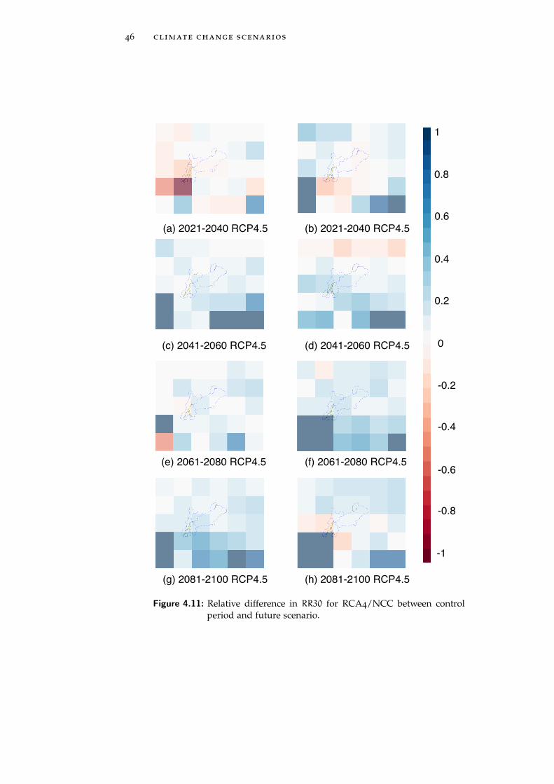
shows a slight increase in precipitation over most of the cells com-pared to the control period. However, precipitation is predicted todecrease in other cells of the domain. Unlike temperature, with pre-cipitation we can not detect a clear trend, and the RCP8.5 is not an in-tensification of the RCP4.5, but predicts different temporal evolutions.An indicator describing changes in the frequency of heavy precipita-tion events is RR30 [Frei et al., 1998]. The RR30 index represents thefrequency of days with a precipitation over 30 mm of rain
RR30 = Ndays(rain>30mm)/Ndays
where Ndays is the total number of days and Ndays(rain>30mm)
is the number of days in which the precipitation exceeds 30 mm. InFigure 4.11 the relative difference of the indicator RR30 is plottedover the domain during the four sub-periods already described. Wecan see that an increase of approximately 20% in heavy precipitationevents is expected over the domain of interest in the majority of thecells for the model RCA4/NCC fed by the RCP4.5 scenario, while forthe RCP8.5 scenario this increase goes up to 30%. The two RCPs areconcordant in predicting an increase of heavy precipitation eventsand the RCP8.5 shows a more intense rise compared to the RCP4.5.

44 climate change scenarios
(a) 2021-2040 RCP4.5!
(h) 2081-2100 RCP4.5!
(d) 2041-2060 RCP4.5!
(f) 2061-2080 RCP4.5!
(c) 2041-2060 RCP4.5!
(g) 2081-2100 RCP4.5!
(e) 2061-2080 RCP4.5!
(b) 2021-2040 RCP4.5!
6!
5!
4!
3!
2!
1!
0!
Figure 4.9: Changes in mean temperature (° C) of RCA4/NCC between con-trol period and future scenario.

4.3 statistical analysis of the euro-cordex scenarios 45
(a) 2021-2040 RCP4.5!
(h) 2081-2100 RCP4.5!
(d) 2041-2060 RCP4.5!
(f) 2061-2080 RCP4.5!
(c) 2041-2060 RCP4.5!
(g) 2081-2100 RCP4.5!
(e) 2061-2080 RCP4.5!
(b) 2021-2040 RCP4.5!
0.5!
0.4!
0.3!
0.2!
0.1!
0!
-0.1!
-0.2!
-0.3!
-0.4!
-0.5!
Figure 4.10: Relative difference in mean precipitation (-) for RCA4/NCCbetween control period and future scenario.
46 climate change scenarios
(a) 2021-2040 RCP4.5!
(h) 2081-2100 RCP4.5!
(d) 2041-2060 RCP4.5!
(f) 2061-2080 RCP4.5!
(c) 2041-2060 RCP4.5!
(g) 2081-2100 RCP4.5!
(e) 2061-2080 RCP4.5!
(b) 2021-2040 RCP4.5!
1!
0.8!
0.6!
0.4!
0.2!
0!
-0.2!
-0.4!
-0.6!
-0.8!
-1!
Figure 4.11: Relative difference in RR30 for RCA4/NCC between controlperiod and future scenario.

4.3 statistical analysis of the euro-cordex scenarios 47
In this thesis, among the several analysis methods, we use the MASH
tool [Anghileri et al., 2014]. The MASH is a novel visual method, whichallows detecting trends in climate and hydrological variables, show-ing changes in seasonal patterns. The MASH consists of averaging thedaily values over consecutive days in the same year (considering al-ways 365 days per year) and over the same days for consecutive years,shifting progressively the horizon. The MASH can therefore be consid-ered as the following matrix
MASH =
µ1,1 µ1,2 ... µ1,Nh
µ2,1 µ2,2 ... µ2,Nh
... ... ... ...
µ365,1 µ365,2 ... µ365,Nh
where each element is the average daily flow on the tth day of theyear over the hth horizon, calculated as follows
µt,h = meany∈[h,h+Y−1]
[mean
d∈[t−w,t+w]Xd,y
]where Xd,y is the value of the variable of interest at day d and year y.Y is a parameter representing the number of years averaged together,in the formula from year h to year h+ Y − 1. w is the parameter re-lated to the day-to-day variability and total number of days averagedtogether is 2 ∗w+ 1 (from day t−w to day t+w, as shown in the for-mula). In our analysis we set the parameters Y to 20, considered to belarge enough to filter out the natural climate variability. The parame-ter w, related to the daily variability, was set to 15 (namely averagingover 31 days), considered to be a good compromise between filter-ing the day-to-day variability and preserving the natural seasonalpatterns. Figures 4.12, 4.13, 4.14, and 4.15 show the MASH plots fortwo climate scenarios of the variables of temperature and precipita-tion under the RCP4.5 and RCP8.5 over the XXI century time horizon.The two scenarios REMO/MPI and RACMO/ICHEC are chosen asrepresentative of the entire ensemble. The graphs of the remainingscenarios are reported in Appendix A. Within the scenario time hori-zon, we see the increase in temperature, which has a positive signin all seasons and is always higher in graphs related to the RCP8.5(Figures 4.12b and 4.14b). Regarding the precipitation, most of thescenarios analyzed show a decrease in the summer months and anincrease in winter, as shown in Figures 4.13a to 4.15b for the repre-sentative scenarios REMO/MPI and RACMO/ICHEC. The intensityof this seasonal shift is higher for the RCP8.5, as shown for instancein Figure 4.13b for the scenario REMO/MPI. Similar changes werealready detected in other works on the Alpine region, for example inGobiet et al. [2014].

48 climate change scenarios
0 50 100 150 200 250 300 350
−10
−5
0
5
10
15
20
25
[Calendar Unit]
[°C
]
2008 to 2027
2018 to 2037
2028 to 2047
2038 to 2057
2048 to 2067
2058 to 2077
2068 to 2087
2078 to 2097
(a) RCP4.5
0 50 100 150 200 250 300 350
−10
−5
0
5
10
15
20
25
[Calendar Unit]
[°C
]
2008 to 2027
2018 to 2037
2028 to 2047
2038 to 2057
2048 to 2067
2058 to 2077
2068 to 2087
2078 to 2097
(b) RCP8.5
Figure 4.12: Temperature MASH of REMO/MPI

4.3 statistical analysis of the euro-cordex scenarios 49
0 50 100 150 200 250 300 350
2
3
4
5
6
7
8
9
Calendar Unit
[mm
/da
y]
2008 to 2027
2018 to 2037
2028 to 2047
2038 to 2057
2048 to 2067
2058 to 2077
2068 to 2087
2078 to 2097
(a) RCP4.5
0 50 100 150 200 250 300 350
2
3
4
5
6
7
8
9
Calendar Unit
[mm
/da
y]
2008 to 2027
2018 to 2037
2028 to 2047
2038 to 2057
2048 to 2067
2058 to 2077
2068 to 2087
2078 to 2097
(b) RCP8.5
Figure 4.13: Precipitation MASH of REMO/MPI

50 climate change scenarios
0 50 100 150 200 250 300 350
−10
−5
0
5
10
15
20
25
[Calendar Unit]
[°C
]
2008 to 2027
2018 to 2037
2028 to 2047
2038 to 2057
2048 to 2067
2058 to 2077
2068 to 2087
2078 to 2097
(a) RCP4.5
0 50 100 150 200 250 300 350
−10
−5
0
5
10
15
20
25
[Calendar Unit]
[°C
]
2008 to 2027
2018 to 2037
2028 to 2047
2038 to 2057
2048 to 2067
2058 to 2077
2068 to 2087
2078 to 2097
(b) RCP8.5
Figure 4.14: Temperature MASH of RACMO/ICHEC

4.3 statistical analysis of the euro-cordex scenarios 51
0 50 100 150 200 250 300 350
2
3
4
5
6
7
8
9
Calendar Unit
[mm
/da
y]
2008 to 2027
2018 to 2037
2028 to 2047
2038 to 2057
2048 to 2067
2058 to 2077
2068 to 2087
2078 to 2097
(a) RCP4.5
0 50 100 150 200 250 300 350
2
3
4
5
6
7
8
9
Calendar Unit
[mm
/da
y]
2008 to 2027
2018 to 2037
2028 to 2047
2038 to 2057
2048 to 2067
2058 to 2077
2068 to 2087
2078 to 2097
(b) RCP8.5
Figure 4.15: Precipitation MASH of RACMO/ICHEC


5S TAT I S T I C A L D O W N S C A L I N G
5.1 historical climate observations
As described in Chapter 2, in order to downscale the climate changescenarios we need historical climate observations on a sufficientlylong time horizon. The historical observations used in this analy-sis are taken from the temperature stations belonging to ARPA andfrom a high-resolution grid precipitation dataset distributed by theSwiss Federal Office of Meteorology and Climatology, MeteoSwiss(Figure 5.1). The ARPA meteorological network consists of several sta-tions with daily and hourly time resolution located in Lombardia. Wechoose the stations with a long time series and with a good recordquality. The results of this selection are the time series of mean dailytemperature from 1988 to 2001 recorded in Sondrio, Chiavenna, Scaisand Santa Caterina (Figure 5.1). The precipitation grid dataset is theresult of a trans-national analysis that has been carried out collectinginformation from precipitation gauges over the Alpine area in sevencountries (Italy, Switzerland, Austria, Germany, France, Slovenia, andCroatia) with approximately 5500 measurements per day from 1971
to 2008 [Isotta et al., 2014]. The result is a high-resolution grid (5 Km),over a domain that encompasses approximately 1200 km from Franceto Austria and over 700 km from southern Germany to northern Italy,including parts of the territory of Slovenia and Croatia. The grid cellsthat intersect the Lake Como catchment are 247 (Figure 5.1).
5.2 statistical downscaling via quantile mapping
We adopt a simple and efficient procedure to carry out the down-scaling of the climate model outputs. We associate the closest EURO-CORDEX cell to every single ARPA weather stations and grid cell ofthe Alpine dataset. We carry out this assignment twice, once withEURO-CORDEX coarser resolution (0.44 degree) and once with thefiner one (0.11 degree). We perform the assignment in order to beable to carry out the downscaling of the climate model on every pointof the Alpine precipitation grid and on every temperature gauge. Af-ter assigning a predictor (large-scale output of the climate models) toevery predictand (small scale variable of the climate observations),the Quantile Mapping method is applied, computing the quantilecurves. As an example, Figure 5.2 shows the quantile-quantile plotof the EURO-CORDEX cell in the EUR-44 resolution over the period1988-2001 (model RCA4/MIROC) and the temperature time series of
53

54 statistical downscaling
Figure 5.1: Precipitation Grid Cells and ARPA Temperature stations
the nearest weather station (Chiavenna). We see that, in this case, theclimate model underestimates the observations and it does it moreintensely for low temperature.
5.3 statistical analysis of the downscaled scenarios
After the downscaling phase a brief statistical analysis is carried out.The goal of this part of the work is to examine if the downscaledscenarios are consistent with the original climate model outputs andif the expected effects of the bias removal are observed. The bias re-moval should reduce the differences in the average behaviour amongthe model scenarios in the control period and consequently also in thefuture scenarios, if we suppose that the model errors of the GCM/RCMare constant over the past and over the future. This effect can be seenin Figures 5.3 and 5.4, where the mean precipitation and the meantemperature of all the model scenarios are plotted on a graph. Com-pared to what shown in Chapter 4, we see that the behaviour of thedifferent models over the future scenario, even considering both theRCPs, is less spread (w.r.t. Figures 4.7 and 4.8) and contained in asmaller region of the graph with mean temperature between 7° Cand 10° C. The same range for mean daily precipitation varies ap-proximately from 3.35 to 4.25 mm/d, corresponding to yearly precip-itation values between 1200 and 1550 mm/y.

5.3 statistical analysis of the downscaled scenarios 55
−20 −15 −10 −5 0 5 10 15
−20
−15
−10
−5
0
5
10
15
Backcast
Ob
se
rva
tio
n
Figure 5.2: Quantile-quantile plot of the Chiavenna temperature station andits predictor for the model RCA4/MIROC forced by the RCP4.5

56 statistical downscaling
0 2 4 6 8 103
3.5
4
4.5
5
5.5
6
mean temperature [°C]
me
an
pre
cip
ita
tio
n [
mm
/d]
RCP4.5 SCENARIO DOWNSCALED
hisRCA4 MIROC
RCA4 NCC
RCA4 NOAARCA4 CCC
RCA4 CNRMRCA4 ICHEC
CCLM MPICCLM ICHEC
HIRHAM ICHEC
RACMO ICHECREMO MPI
Figure 5.3: Mean values of temperature (x-axis) and precipitation (y-axis)for all the dowscaled scenarios fed by the RCP4.5 over the timehorizon 2006-2100. Different GCMs are represented by differentsymbols, while different RCMs are represented by different col-ors.
0 2 4 6 8 103
3.5
4
4.5
5
5.5
6
mean temperature [°C]
me
an
pre
cip
ita
tio
n [
mm
/d]
RCP8.5 SCENARIO DOWNSCALED
hisRCA4 MIROC
RCA4 NCC
RCA4 NOAARCA4 CCC
RCA4 CNRMRCA4 ICHEC
CCLM MPICCLM ICHEC
HIRHAM ICHEC
RACMO ICHECREMO MPI
Figure 5.4: Mean values of temperature (x-axis) and precipitation (y-axis)for all the dowscaled scenarios fed by the RCP8.5 over the timehorizon 2006-2100. Different GCMs are represented by differentsymbols, while different RCMs are represented by different col-ors.
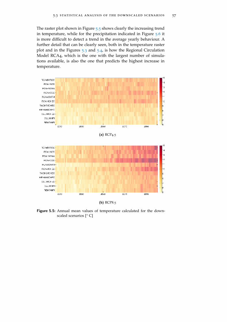
5.3 statistical analysis of the downscaled scenarios 57
The raster plot shown in Figure 5.5 shows clearly the increasing trendin temperature, while for the precipitation indicated in Figure 5.6 itis more difficult to detect a trend in the average yearly behaviour. Afurther detail that can be clearly seen, both in the temperature rasterplot and in the Figures 5.3 and 5.4, is how the Regional CirculationModel RCA4, which is the one with the largest number of simula-tions available, is also the one that predicts the highest increase intemperature.
(a) RCP4.5
0
(b) RCP8.5
Figure 5.5: Annual mean values of temperature calculated for the down-scaled scenarios [° C]

58 statistical downscaling
(a) RCP4.5
(b) RCP8.5
Figure 5.6: Annual mean values of precipitation calculated for the down-scaled scenarios [mm/d]

6H Y D R O L O G I C A L M O D E L L I N G
6.1 topkapi-eth setup
The following step of the thesis involves the understanding of the cli-mate change impact on the hydrology of the Lake Como catchment.As already shown in Chapter 2, in order to fully understand the re-lationship between changes in climate and hydrological regime, it isnecessary to consider a model that describes the physical processesaffecting the hydrological cycle in an Alpine environment (e.g., evapo-transpiration, snowmelt, and glacier dynamics). We use Topkapi-ETH(TE), a physically-based and fully distributed hydrological model thatprovides the possibility to account for anthropogenic infrastructuressuch as reservoirs and river diversions, which play a key role in thestudy site. The importance of employing a spatially distributed modelis due to the possibility of assessing the hydrological response toclimate change in every single area of the catchment, allowing spa-tial analyses on river network, glaciers, and hydropower reservoirs.Moreover, the spatial analysis could be extended to the assessmentof mitigation measures on other water-related activities, for instanceflood protection, ecosystem conservation, and agriculture. TE repre-sents a good trade-off between computational time, required to runthe model, and a thorough description of hydrological processes. Weimplement the model on a spatial grid of 250 m, which representsa good compromise between a reasonable computational time (giventhe large number of climate scenarios which has to be simulated) andan accurate topographic description of the complex Alpine terrain.The model requires a description of several spatial characteristics ofthe catchment: a Digital Elevation Model (DEM), a soil map, a landcover map, a glaciers map, a glaciers depth map, and the maps of theThiessen polygons of the weather stations of temperature, precipita-tion, and cloud cover transmissivity.
6.1.1 Digital Elevation Model
The Digital Elevation Model is obtained from the Shuttle Radar To-pography Mission (SRTM), a space mission coordinated by NationalAeronautics and Space Administration (NASA) and National Geospatial-Intelligence Agency (NGA). The data has an original resolution of 1
arc-second (approximately 30 m) and was retrieved in GeoTIFF for-mat from the United States Geological Survey (USGS) website, see Fig-
59
60 hydrological modelling
ure 6.1. A DEM is required in Topkapi-ETH to extract informationabout the catchment area, the flow direction, and the river network.
6.1.2 Soil Map
Considering the location of the basin, which extends over two coun-tries, the information concerning soil is obtained from two differentsources and then merged together within a Geographical Informa-tion System (GIS). For the Italian part of the domain, the soil mapis provided by the local ARPA. For the Swiss part we retrieve theBodeneignuskarte from the Swiss Federal Agriculture Office (Bunde-samt für Landwirtschaft), see Figure 6.2. To every soil class are asso-ciated the parameters regarding thickness and hydraulic properties(see Section 6.2).
6.1.3 Land Cover Map
Also for the land cover, we obtaine the information from two differentsources. For the Italian part of the basin, the used land cover map isthe Destinazione d’Uso dei Suoli Agricoli e Forestali (DUSAF), a prod-uct developed by the local ARPA. For the Swiss part of the domainthe Corine Land Cover, a European land cover map less detailed thanDUSAF, is the best information available, see Figure 6.3. Parameters asthe Manning coefficients and the monthly evapotranspiration coeffi-cients are associated in Topkapi-ETH to every class of the land covermap (see Section 6.2).
6.1.4 Glacier Map
A glaciers map is provided by the local ARPA. Since there is no avail-able information on the glaciers’ ice thickness across the whole do-main, this data is estimated from the area, with an empirical formulaand assuming an uniform ice thickness, as follows [Fatichi et al., 2013;Farinotti et al., 2009]
hice = 33A0.36
where A[km2] is the area of the single glacier and hice[m] representsits ice thickness. This assumption on the initial ice thickness is neces-sary to evaluate the potential glacier retreat due to melting, see Figure6.4.
6.1.5 Thiessen Polygons for Temperature, Precipitation and Cloud CoverTransmissivity
Since Topkapi-ETH requires spatial inputs, we transform the tempera-ture, precipitation, and Cloud Cover Transmissivity time series from

6.1 topkapi-eth setup 61
points to maps using the Thiessen polygons. As already shown inChapter 5, the temperature time series are taken from the historicalARPA stations and the Thiessen polygons are computed in a GIS en-vironment, see Figure 6.5. Figure 6.6 shows the map obtained trans-forming with Thiessen polygons the points of the Alpine precipitationgrid. The best available information on Cloud Cover Transmissivity isprovided by a single station, at the Samedan Airport, which is locatedslightly outside the catchment. We thus consider only one Thiessenpolygon over the entire domain.
6.1.6 Reservoirs
Figure 6.7 shows the hydropower reservoirs included in the analysisas well as the Lake Como. Besides the location and the spatial extentfor each reservoir, Topkapi-ETH further requires a level/storage anda level/max-outflow curve. Moreover, Topkapi-ETH allows includingsimple reservoir operational rules, which can be defined separatelyfor each artificial lake.
6.1.7 Groundwater Depth
The groundwater depth is an optional input in Topkapi-ETH that sim-ulates the groundwater flow with an approach described in Liu et al.[2005], accounting for percolation to deep soil layers and groundwa-ter flows. In our analysis we define two groundwater classes, one, 8
meters deep, at lower altitudes along the river network and one, 2
meters deep, for the rest of the catchment, as shown in Figure 6.8.

62 hydrological modelling
Figure 6.1: DEM of the catchment obtained with Topkapi-ETH
Figure 6.2: Soil Type Map

6.1 topkapi-eth setup 63
Figure 6.3: Land Cover Map
Figure 6.4: Glaciers Depth Map

64 hydrological modelling
Figure 6.5: Temperature Thiessen Polygons Map
Figure 6.6: Precipitation Thiessen Polygons Map

6.1 topkapi-eth setup 65
Figure 6.7: Reservoirs map
Figure 6.8: Groundwater Depth Map

66 hydrological modelling
6.2 calibration and validation
As described in Chapter 2, Topkapi-ETH requires as input time seriesof precipitation, temperature and cloud cover transmissivity. As al-ready said, we retrieve the former two from the Alpine precipitationgrid distributed by MeteoSwiss [Isotta et al., 2014] and the ARPA tem-perature gauges. Cloud Cover Transmissivity (CCT) is obtained by thesolar radiation collected in Samedan, located approximately 25 Kmoutside the catchment.Topkapi-ETH can simulate the reservoirs operation defining a “rulecurve” , i.e., a reference trajectory that can be defined as the trajectoryof the storage during a normal hydrological year [Soncini-Sessa et al., 2007].In Topkapi-ETH the “rule curve” is implemented setting the reservoiroutflow to zero, when the storage is lower than the reference trajec-tory, and to the maximum value allowed, when the storage is biggerthan the reference trajectory. This simple operative rule is far fromcorrectly describing the behaviour of the reservoir manager, whosedecisions are based on other factors (e.g., day of the week, forecastedinflow, and electricity price). Nevertheless, the employment of a “rulecurve” can reproduce the general effect of the reservoirs on the hy-drology, which is basically moving water volumes among seasons.The annual reference trajectory for each reservoir is calculated fromthe historical observations of storages for the period 2006-2012. Wecompute a cyclostationary mean across the 2006-2012 time horizon,smoothing the values with a mobile window of 11 days.We consider the section of Fuentes, located on the River Adda at themouth to the Lake Como for the calibration and validation of the hy-drological model (Figure 6.9). Observations at Fuentes gauge stationare the most reliable observations of streamflow across the catchment.The time series used for the calibration is provided by ARPA, compris-ing a period of 41 years (1971-2011). The calibration of Topkapi-ETHis initially performed using literature values for the parameters refer-ring to soil and land use properties. In fact, all its parameters have aphysical meaning and are associated to particular classes. For exam-ple, the physical properties of the soil, such as hydraulic conductivity,can vary depending on its composition. This initial parameter set isthen slightly adjusted to improve the performances of the model withregard to the available streamflow time series. More precisely, we per-form a manual calibration of the following parameters:
• Manning coefficient:it is the surface roughness coefficient and depends on the landcover types, defining the resistance to flows.
• Monthly evapotranspiration coefficients:they represent the evapotranspiration factors for each land cover

6.2 calibration and validation 67
Figure 6.9: Fuentes location on the catchment. The Figure shows the riversection of Fuentes, where we did the calibration, the Lake Comoand the River Adda.
type and month. The values are generally lower in the coldmonths and higher in spring and summer.
• Soil Depth:it represents the soil thickness of the two layers defined in Topkapi-ETH.
• Residual water content ratio (ThetaR) and water content ratioat saturation (ThetaS):they represent the water content characteristics of the two soillayers.
• Horizontal (KsH) and vertical (KsV) hydraulic conductivity:they are a measure of saturated soil ability to transmit waterwhen subjected to a hydraulic gradient. These parameters varywithin a wide range of orders of magnitude, depending on thesoil type. For instance, clay has a lower hydraulic conductivityat saturation than sand.
The calibration is performed w.r.t. three performance indices: Thecoefficient of determination (R2), the root of the mean square error(RMSE), and Kling-Gupta Efficiency (KGE). R2 represents the portionof the total variance of the observed data that can be explained by themodel
R2 = 1−var(yobs,t − ymod,t)
var(yobs,t)
68 hydrological modelling
where yobs,t and ymod,t are the observed and modelled time seriesrespectively. As known, R2 is very sensitive to outliers and not sensi-tive to proportional and additive variations, so it might be misleading,for instance, when dealing with systematic underestimations or over-estimation of the streamflow [Legates and McCabe, 1999].
RMSE represents the standard deviation of the difference betweenobserved and predicted values and it is widely used in hydrologicalmodelling [Legates and McCabe, 1999]
RMSE =
√∑Nt=1(yobs,t − ymod,t)2
N
where yobs,t and ymod,t are the observed and modelled values attime t respectively.
KGE is an alternative measure of performance for hydrological mod-els which aims to overcome the traditional problems associated withcalibration, for instance variability underestimation and low sensitiv-ity to proportional and additive variations [Gupta et al., 2009]
α =σmod
σobs, β =
µmod
µobs, r =
√R2
ED =√(r− 1)2 + (α− 1)2 + (β− 1)2
KGE = 1− ED
where σobs and σmod are the standard deviations of observed andmodelled time series, while µobs and µmod are the two means.
We calibrate the model on the period 1988-1994, considering the firsttwo years as warm-up period, and we validate it on the period 1997-1999. The final performance values of the calibration are: R2 = 0.72,RMSE = 103.30 m3/s, and KGE = 0.74 (Table 6.1). Figure 6.10 showsthe comparison between modelled and observed time series over theperiod 1990-1994 (Figure 6.10a) and over the year 1992 (Figure 6.10b).These values are acceptable considering the wide domain, the dailytime step, and the spatial time resolution adopted (250 m). As visibleespecially in the zoom-in over the year 1992 (Figure 6.10b), there areweekly fluctuations caused by the operations of the reservoirs thatrelease smaller volumes of water during the weekends. Those fluc-tuations are visible especially in the winter months as the naturalstreamflow is lower. In order to filter the extra variability caused bythe hydropower operations, we calculate the performance metrics onthe weekly average streamflow, instead of on the daily one (Table 6.1).As expected, all the metrics improve when computed on a weeklybasis.

6.3 hydrological scenarios analysis 69
Calib. Daily Valid. Daily Calib. Weekly Valid. Weekly
R2[−] 0.72 0.69 0.79 0.79
RMSE[m3/s] 103.30 59.82 37.18 49.94
KGE[−] 0.74 0.77 0.81 0.84
Table 6.1: Calibration performance summary: R2, RMSE, and KGE over thecalibration and validation periods
6.3 hydrological scenarios analysis
6.3.1 Experiment Setup
In order to assess the impact of climate change on the hydrology ofthe catchment, we carry out the simulations of Topkapi-ETH fed bythe downscaled time series of temperature and precipitation retrievedfrom the EURO-CORDEX scenarios. As already discussed in Chapter4, we consider combinations of five RCMs (REMO, RCA4, RACMO,HIRHAM, and CCLM) and seven GCMs (MPI, NOAA, NCC, ICHEC,MIROC, CCC, and CNRM) forced by two Representative Concentra-tion Pathways (RCP4.5 and RCP8.5), for a total of 22 scenarios over theperiod 2006-2100 (not all the combinations are available). Aside the 22
simulations of the future scenarios, we also carry out 11 simulationsfed by the downscaled variables over the control period, in order tosimulate the current hydrology. The total computational time is ap-proximately 90 hours. As for the reservoir operation, we perform abusiness-as-usual analysis, supposing that the rule curves will remainthe historical ones also in the future.
6.3.2 Impact of Climate Change on Streamflows
We carry out a statistical analysis of the hydrological model output,in order to assess how the predicted changes in temperature and pre-cipitation reflect on the streamflows in the catchment. As alreadydone for the climate scenarios, we use boxplots to summarize themain statistics (Figures 6.11, 6.12, and 6.13). After that, we calculatethe cyclostationary mean of all the scenarios over the CORDEX time-horizon. Finally, we compute MASH plots of all the hydrological sce-narios. In this Chapter we present only the results relative to the sce-narios REMO/MPI and RACMO/ICHEC, considered representativeof the entire ensemble (for the MASH of the other scenarios see Ap-pendix B).

70 hydrological modelling
1990 1991 1992 1993 19940
100
200
300
400
500
600
700
800
time [d]
str
eam
flow
[m
3/s
]
Fuentes 1990−1994
Observed
Modelled
(a) 1990-1994
J F M A M J J A S O N D0
50
100
150
200
250
300
350
400
time [d]
str
eam
flow
[m
3/s
]
Fuentes 1992
Observed
Modelled
(b) Zoom-in 1992
Figure 6.10: Observed and modelled streamflows at the river section ofFuentes

6.3 hydrological scenarios analysis 71
0
50
100
150
200
250
300
RC
A4
MIR
OC
RC
A4
NC
C
RC
A4
NO
AA
RC
A4
CC
C
RC
A4
CN
RM
RC
A4
IC
HE
C
RA
CM
O I
CH
EC
HIR
AM
IC
HE
C
CC
LM
IC
HE
C
CC
LM
MP
I
RE
MO
MP
I
[m3/s
]
FUENTES STREAMFLOW CONTROL PERIOD
Figure 6.11: Boxplot Streamflow Fuentes Control Period
As already seen with the climate variables, looking only at the stan-dard statistics shown in the boxplots, it is difficult to determine con-cordant changes in hydrology between the control period and thefuture scenarios (Boxplots 6.11 to 6.13). Figure 6.11 shows that allthe scenarios have similar statistics, besides the CCLM/MPI, whichshows a slightly higher variability. Figure 6.14, 6.15, and 6.16 showthe cyclostationary averages of the streamflows at Fuentes, computedover the control period and then over the future horizon for all the cli-mate scenarios forced by RCP4.5 and 8.5 respectively. Looking at thescattered distribution of the lines on the graphs we perceive the highuncertainty related to the climate models that reflects on the hydro-logical scenarios. Over the control period the climate scenarios havingCCLM as RCM, show a different pattern with a late snowmelt peakand lower intensity in the autumn flows. The cyclostationary meanof the simulation outputs over the future scenarios (Figures 6.15 and6.16) show a high variability, among the different models, both in win-ter and summer streamflows and in the time of the snowmelt peak.

72 hydrological modelling
0
50
100
150
200
250
300
RC
A4
MIR
OC
RC
A4
NC
C
RC
A4
NO
AA
RC
A4
CC
C
RC
A4
CN
RM
RC
A4
IC
HE
C
RA
CM
O I
CH
EC
HIR
AM
IC
HE
C
CC
LM
IC
HE
C
CC
LM
MP
I
RE
MO
MP
I
[m3/s
]
FUENTES STREAMFLOW RCP4.5
Figure 6.12: Boxplot Streamflow Fuentes RCP4.5
0
50
100
150
200
250
300
RC
A4
MIR
OC
RC
A4
NC
C
RC
A4
NO
AA
RC
A4
CC
C
RC
A4
CN
RM
RC
A4
IC
HE
C
RA
CM
O I
CH
EC
HIR
AM
IC
HE
C
CC
LM
IC
HE
C
CC
LM
MP
I
RE
MO
MP
I
[m3/s
]
FUENTES STREAMFLOW RCP8.5
Figure 6.13: Boxplot Streamflow Fuentes RCP8.5

6.3 hydrological scenarios analysis 73
0 50 100 150 200 250 300 3500
50
100
150
200
250
Caledar unit
Str
eam
flow
[m
3/s
]
RCA4 MIROC
RCA4 NCC
RCA4 NOAA
RCA4 CCC
RCA4 CNRM
RCA4 ICHEC
RACMO ICHEC
HIRHAM ICHEC
CCLM ICHEC
CCLM MPI
REMO MPI
Figure 6.14: Trajectories Fuentes Control Period
0 50 100 150 200 250 300 3500
50
100
150
200
250
Caledar unit
Str
eam
flow
[m
3/s
]
RCA4 MIROC
RCA4 NCC
RCA4 NOAA
RCA4 CCC
RCA4 CNRM
RCA4 ICHEC
RACMO ICHEC
HIRHAM ICHEC
CCLM ICHEC
CCLM MPI
REMO MPI
Figure 6.15: Trajectories Fuentes RCP4.5

74 hydrological modelling
0 50 100 150 200 250 300 3500
50
100
150
200
250
Caledar unit
Str
eam
flow
[m
3/s
]
RCA4 MIROC
RCA4 NCC
RCA4 NOAA
RCA4 CCC
RCA4 CNRM
RCA4 ICHEC
RACMO ICHEC
HIRHAM ICHEC
CCLM ICHEC
CCLM MPI
REMO MPI
Figure 6.16: Trajectories Fuentes RCP8.5

6.3 hydrological scenarios analysis 75
As already done in Chapter 4 for the climate variables, we apply theMASH tool also to the hydrological scenarios, to detect changes in theseasonal pattern of streamflow over the century. In order to be consis-tent with the previous analysis, the parameters used are Y = 20 andw = 15. As already mentioned for the climate variables, these valuesrepresent a good trade-off between filtering out the daily variabilityand preserving seasonal patterns. In this section we show the MASH
relative to the scenarios REMO/MPI and RACMO/ICHEC, taken asrepresentative of the whole ensemble (the graphs related to the otherscenarios are fully shown in Appendix B). The main trends visiblein Figures 6.17 and 6.18 are an increase in winter streamflow and adecrease in summer streamflow. Other aspects observed in most ofthe scenarios are a shift towards an earlier snowmelt peak and a de-layed secondary autumn peak. Figure 6.17 shows the MASH for theREMO/MPI scenario, where the mean rise in winter streamflow be-tween the first and last two decades of simulation (2008-2027 and2081-2100) amounts to 26.6% for RCP4.5 and to 43.14% for RCP8.5. Onthe contrary there is a mean summer decrease of 7.3% and 23.1% re-spectively. The changes detected in the RACMO/ICHEC scenario are19.6% and 31.6% of winter increase for RCPs 4.5 and 8.5, and reduc-tions of 5.5% and 14.9% during the summer months (Figure 6.18). Thesnowmelt peak is expected up to one month earlier for the RCP8.5 insome scenarios, while this anticipation is lower for the RCP4.5. Theshift towards a later autumn peak can be seen under both the RCPs,as shown in Figure 6.17, representing the outputs of the model RE-MO/MPI fed by RCP4.5 and RCP8.5.

76 hydrological modelling
0 50 100 150 200 250 300 3500
50
100
150
200
250
Calendar Unit
[m3/s
]
2008 to 2027
2018 to 2037
2028 to 2047
2038 to 2057
2048 to 2067
2058 to 2077
2068 to 2087
2078 to 2097
(a) RCP4.5
0 50 100 150 200 250 300 3500
50
100
150
200
250
Calendar Unit
[m3/s
]
2008 to 2027
2018 to 2037
2028 to 2047
2038 to 2057
2048 to 2067
2058 to 2077
2068 to 2087
2078 to 2097
(b) RCP8.5
Figure 6.17: REMO/MPI, Fuentes streamflow

6.3 hydrological scenarios analysis 77
0 50 100 150 200 250 300 3500
50
100
150
200
250
Calendar Unit
[m3/s
]
2008 to 2027
2018 to 2037
2028 to 2047
2038 to 2057
2048 to 2067
2058 to 2077
2068 to 2087
2078 to 2097
(a) RCP4.5
0 50 100 150 200 250 300 3500
50
100
150
200
250
Calendar Unit
[m3/s
]
2008 to 2027
2018 to 2037
2028 to 2047
2038 to 2057
2048 to 2067
2058 to 2077
2068 to 2087
2078 to 2097
(b) RCP8.5
Figure 6.18: RACMO/ICHEC, Fuentes streamflow

78 hydrological modelling
Figure 6.19: Glacier Map of the catchment with highlighted the ForniGlacier (in blue) and the Val Lia / Cardonnè Glacier (in red).
6.3.3 Impact of Climate Change on Glaciers
Glaciers retreat strongly affects the hydrology in high-elevation catch-ments [Fatichi et al., 2013]. In the Lake Como basin the glaciers sur-face is only 1.4% of the total area, considering the catchment closedat Olginate, but this value considerably increases if taking into ac-count only the areas nearby the Alpine reservoirs. San Giacomo andCancano reservoirs, for instance, are fed by highly glacierized areasthrough artificial channels. As an example, we analyzed the ForniGlacier, the Val Lia, and the Cardonnè Glaciers. The Forni Glacieris the biggest glacier in the Italian Alps and it is located in the Or-tles–Cevedale Group at an average altitude of 3096 m a.s.l.. Con-trarily, the Val Lia and Cardonnè Glaciers are considerably smallerand located on average at 2800 m a.s.l. (Figure 6.19). Monitoring theoutput of the two representative scenarios (REMO/MPI and RAC-MO/ICHEC) we see that the smaller and lower glacier shows a con-siderable decrease in yearly discharge (Figures 6.20a and 6.21a). Onthe contrary the glacier of Forni, located at a higher altitude, does notshow relevant signs of retreat in the two climate models, forced bythe RCP4.5 (Figures 6.20b and 6.21b). When forced by the RCP8.5, themodel REMO/MPI shows instead an increase in the discharge of theForni Glacier, during the last decades of the century (Figure 6.20b,blue line), which might be caused by the initial retreat, which usu-ally produces higher discharges [Jansson et al., 2003]. Similar resultson the elevation dependent glacier response to climate change whereobtained by Fatichi et al. [2013]. The sum of the discharges from allthe glaciers considered in the catchment shows a decrease of 20% forRCP4.5 and of 32.7% for RCP8.5 comparing the last part of the century(2071-2100) to the control period, when taking into account all the 22
scenarios of the analysis.
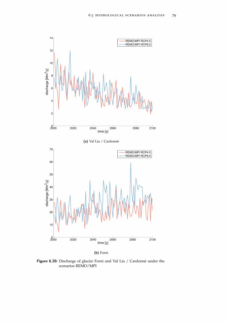
6.3 hydrological scenarios analysis 79
2000 2020 2040 2060 2080 21000
2
4
6
8
10
12
14
time [y]
dis
charg
e [M
m3/y
]
Val Lia / Cardonnè
REMO/MPI RCP4.5REMO/MPI RCP8.5
(a) Val Lia / Cardonnè
2000 2020 2040 2060 2080 21000
10
20
30
40
50
60
70
time [y]
dis
charg
e [M
m3/y
]
Forni
REMO/MPI RCP4.5REMO/MPI RCP8.5
(b) Forni
Figure 6.20: Discharge of glacier Forni and Val Lia / Cardonnè under thescenarios REMO/MPI

80 hydrological modelling
2000 2020 2040 2060 2080 21000
2
4
6
8
10
12
14
time [y]
dis
charg
e [M
m3/y
]
Val Lia / Cardonnè
RACMO/ICHEC RCP4.5RACMO/ICHEC RCP8.5
(a) Val Lia / Cardonnè
2000 2020 2040 2060 2080 21000
10
20
30
40
50
60
70
time [y]
dis
charg
e [M
m3/y
]
Forni
RACMO/ICHEC RCP4.5RACMO/ICHEC RCP8.5
(b) Forni
Figure 6.21: Discharge of glacier Forni and Val Lia / Cardonnè under thescenarios RACMO/ICHEC

6.3 hydrological scenarios analysis 81
6.3.4 Impact of Climate Change on Reservoir Inflows and Levels
The last objective of our analysis is the understanding of the impactof climate change on the inflow to the reservoirs and the resulting ef-fects on their management. We focus on the biggest reservoirs in thecatchment, i.e., San Giacomo and Cancano reservoirs. Topkapi-ETHallows monitoring the inflow to the reservoir from its tributaries, lakebanks, precipitation, and redistributed snow. The operative rule usedduring the simulation is the one employing a “rule curve”, calculatedwith the historical level observations, as already discussed in Section6.2. The MASH tool is adopted also to analyze the reservoir levels,and to compare it to the target level of the “rule curve”. Figures6.22a and 6.23a show the MASH for the REMO/MPI scenario, indi-cating a 9.8% rise in winter streamflow for RCP4.5 between the firstand last two decades of simulation (2008-2027 and 2081-2100) and20% for RCP8.5. The summer decrease amounts to 8.9% and 22.8%respectively. Figures 6.24a and 6.25a show the changes detected inthe RACMO/ICHEC scenario that amount to 12.8% and 18.5% ofwinter increase for RCPs 4.5 and 8.5, and reductions of 1% and 11%respectively during the summer. Figures 6.22b, 6.23b, 6.24b, and 6.25bshow the water level of the reservoir during the simulations forced bythe reference scenarios. They demonstrate how the hydrological shiftwould affect the levels and the storages of the reservoir. The red linesare the cyclostationary mean calculated over the last decades of thecentury. They show a decrease during summer and autumn in the wa-ter level compared to the blue lines, which are the means calculatedat the beginning of the simulation horizon. A 7 cm gap in the level,shown in Figure 6.23b between the target level and the means com-puted by the MASH over the last decades of simulation (shades of red),indicates approximately 300,000 m3 less storage. The shift towards anearlier snowmelt peak in the REMO/MPI scenario has an impact onthe storage pattern of the reservoir, which tends to be filled earlier.Figures 6.22b and 6.23b show the respective shift in the level pattern,where the red lines in the months of May, June, and July show highervalues than the blue ones. Regarding the scenario RACMO/ICHEC,forced by the RCP4.5, Figure 6.24b shows that, after an initial decrease,in the last part of the century (red lines), the storage of the reservoirseems to get closer to the target level. On the other hand, the samemodel forced by the RCP8.5 shows a clear decrease in the reservoirstorage, caused by an intense reduction in summer and autumn in-flow (Figure 6.25b). The results shown in this Chapter demonstratethat the current storage seasonal patterns can not be reproduced inthe future under climate change conditions. The impossibility of fol-lowing the current seasonal patterns, due to lower summer inflowsand a seasonal hydrological shift, will very likely induce hydropowercompanies to change their strategy.

82 hydrological modelling
0 50 100 150 200 250 300 3500
5
10
15
20
25
Calendar Unit
[m3/s
]
2008 to 2027
2018 to 2037
2028 to 2047
2038 to 2057
2048 to 2067
2058 to 2077
2068 to 2087
2078 to 2097
(a) inflow
(b) level
Figure 6.22: REMO/MPI RCP4.5. MASH of the A2A reservoir inflow andlevel. The target level adopted in the simulation is representedwith a black line.

6.3 hydrological scenarios analysis 83
0 50 100 150 200 250 300 3500
5
10
15
20
25
Calendar Unit
[m3/s
]
2008 to 2027
2018 to 2037
2028 to 2047
2038 to 2057
2048 to 2067
2058 to 2077
2068 to 2087
2078 to 2097
(a) inflow
(b) level
Figure 6.23: REMO/MPI RCP8.5. MASH of the A2A reservoir inflow andlevel. The target level adopted in the simulation is representedwith a black line.
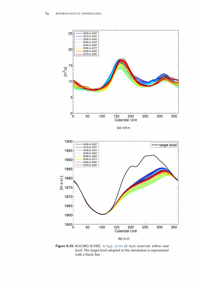
84 hydrological modelling
0 50 100 150 200 250 300 3500
5
10
15
20
25
Calendar Unit
[m3/s
]
2008 to 2027
2018 to 2037
2028 to 2047
2038 to 2057
2048 to 2067
2058 to 2077
2068 to 2087
2078 to 2097
(a) inflow
(b) level
Figure 6.24: RACMO/ICHEC RCP4.5. MASH of A2A reservoir inflow andlevel. The target level adopted in the simulation is representedwith a black line.

6.3 hydrological scenarios analysis 85
0 50 100 150 200 250 300 3500
5
10
15
20
25
Calendar Unit
[m3/s
]
2008 to 2027
2018 to 2037
2028 to 2047
2038 to 2057
2048 to 2067
2058 to 2077
2068 to 2087
2078 to 2097
(a) inflow
(b) level
Figure 6.25: RACMO/ICHEC RCP8.5. MASH of A2A reservoir inflow andlevel. The target level adopted in the simulation is representedwith a black line.


7U N C E RTA I N T Y C H A R A C T E R I Z AT I O N
7.1 “cascade of uncertainty” in climate change impact
studies
The aim of the majority of climate change impact studies is, implicitlyor explicitly, to evaluate or design Policies, Plans, and Programs (PPPs)to reduce or mitigate those impacts. The design and implementa-tion of those PPPs is generally a long and complex process due topolitical and economical reasons. The uncertainty related to climatechange impact studies adds a further degree of complexity to deci-sion making processes, which naturally would prefer certain predic-tions, rather than unclear estimations, in order to assess costs andbenefits of an action (e.g., in the next century the river will reacha specific higher level, therefore we need to build new river banks,of that specific height, in order to avoid floods). Indeed, althoughthe role of uncertainty is well addressed in literature, in most of thereal applications the approach consists of ‘squeezing it out’ from thedecision making process, as if the assumptions of deterministic envi-ronment were satisfied [Soncini-Sessa et al., 2007]. Already more thantwo decades ago Green [1992], quoting a work of Hogan and Jorgen-son [1991], explains how the uncertainty in climate change impacts af-fects and delays the decision making process and how complex is im-plementing costly action on the basis of theoretical predictions of ex-tremely uncertain and never-before experienced events. An importantaspect of uncertainty is its location among other terms related to pre-dictions. Foley [2010], adapting a scheme taken from Stirling [1998],tries to graphically define the concept of “uncertainty” between theones of “risk” and “ignorance”, considering the knowledge about theoutcomes and the knowledge about their likelihood. Figure 7.1 showsthat, with less firm basis for probabilities and less knowledge aboutthe outcomes of a system, scenario analysis should be carried out[Foley, 2010]. Thus, in the majority of climate change impact studies,where the outcomes are not clearly defined and the knowledge abouttheir probability is low, “scenario-based” approaches, as the one usedin this thesis and described in Chapter 2, are recommended.The traditional workflow of climate change impact studies, describedin Chapter 2, is composed by a chain of models. Each of them con-tains, to some extent, uncertain elements, which contribute to increasethe global uncertainty. In Mitchell and Houlme [1999] the concept ofthe “cascade of uncertainty” is introduced. It is described as the ad-
87

88 uncertainty characterization
Figure 7.1: A scheme for defining ‘risk’, ‘uncertainty’ and ‘ignorance’, takenfrom Foley [2010]
ditive process that leads to a fast growing global uncertainty in theoutput of regional climate modelling.This early “cascade” consists of three stages, schematized by triangles(Figure 7.2): the first represents the solar model and socio economicmodel, producing the magnitude of change in the external forcing;the second represents the climate model, producing the magnitude ofclimate change; the third represents the impact model, describing themagnitude of the environmental change. The basis of the trianglesshows the raised uncertainty compared to the vertex, as shown inFigure 7.2.More recently, Wilby and Dessai [2010], describe a similar concept: the“Envelope of Uncertainty” with an increased number of steps throughwhich the uncertainty growths. Obviously, the advancements in thedifferent research fields, in addition to a better understanding of thesystem, also lead to a more complex modelling chain, which pro-duces a more detailed cascade of uncertainty. In this work we show amodified version of the original “cascade of uncertainty”, which fitsto our analysis and case study but can be applied to other climatechange impact studies in the field of water resources management.In the next sections the uncertainty sources related to the differentcomponents shown in Figure 7.3 are described in detail.

7.1 “cascade of uncertainty” in climate change impact studies 89
Figure 7.2: The "Cascade of Uncertainty", from Mitchell and Hulme [1999]
Figure 7.3: The cascade of uncertainty applied to the study case, adaptedfrom Wilby and Dessai [2010]

90 uncertainty characterization
7.1.1 Uncertainty in Radiative Forcing Modelling
The description of the radiative forcing and the resulting definitionof the Representative Concentration Pathways are associated withmany sources of uncertainty. The definition of an emission scenario,which is the cause of the increase in radiative forcing (see Chapter2), involves the understanding of the population growth, the eco-nomic and social development and the future patterns of productionand consumption of energy. In this context, the principal source ofuncertainty stems from the unpredictability of anthropogenic GHGs
emissions and their resultant atmospheric concentration [Foley, 2010].The definition of radiative forcing scenarios, in addition to the emis-sion scenarios (like the old SRES), implies also the complex descrip-tion of the atmospheric GHGs concentrations and of the atmospherechemistry [Moss et al., 2010]. Further important aspects and potentialsources of uncertainty are the climate feedback and possible unex-pected consequences [Foley, 2010], which can arise when GHGs emis-sions interfere with natural climate processes. One example can bethe permafrost melting [Anisimov, 2007]. While it melts, methane andsoil carbon contained in the Arctic and Siberian frozen soil are re-leased, resulting in further global warming. This may obviously leadto a further thawing, amplifying the original signal as a positive feed-back. It has been suggested that methane released from permafrostmay have been the trigger for deglaciation at the end of the Marinoanice age, approximately 635M years ago [Kennedy et al., 2008].
7.1.2 Uncertainty in Global Climate Modelling
In the global climate modelling and in the GCMs design, uncertaintyarises from a limited understanding of the physical processes of theatmosphere that, combined with a coarse spatial resolution, leads toan inappropriate description of the interactions among atmosphere,oceans, cryosphere and land. Especially the parameterization of phys-ical processes taking place at the small scale, for example cloud for-mation, is a highly crucial aspect [Murphy et al., 2004]. Clouds havea variety of effects on both the water balance and the radiation bud-get, which are determined by their height and type [Foley, 2010]. Forinstance, low and thick clouds, such as stratocumulus, have a coolingeffect as they reflect back sunlight, while thin and high clouds such ascirrus, can constitute an extra forcing by trapping outgoing longwaveradiation. All these different effects can not be reproduced in GCMsbecause they happen at a too low spatial resolution.

7.1 “cascade of uncertainty” in climate change impact studies 91
7.1.3 Uncertainty in Regional Climate Modelling
The sources of uncertainty related to Regional Climate Modelling andhence to the RCMs design are not dissimilar to the ones already de-scribed for GCMs. The main difference is the finer resolution, which al-lows RCMs to account for other aspects such as orography, land coverand small atmospheric feature. Since the climate systems have simi-larities with non-linear, chaotic systems [Foley, 2010], unpredictabilitycan arise in two different ways, due to the concepts known in the liter-ature as predictability of the first and of the second kind [Chu, 1998].The first kind of predictability is related with initial conditions, anddescribes the amplification over time of errors in initial conditions. Itrepresents one of the reasons why it is not possible to make accurateweather forecast beyond a week. The second kind of predictability isrelated to boundary conditions. The RCM domains have boundarieswith the surrounding environment, and the model must consider thephysical processes taking place also in this environment. Even thoughit has been less studied than the first kind of predictability, it has beenargued that small variations to boundary conditions can also lead tolarge differences in the future behaviour [Chu, 1998]. For future pro-jections, RCMs usually inherit both initial and boundary conditionsfrom a parent GCM, with procedures known as nesting [Ding et al.,2006; Ju et al., 2007], or double-nesting [Im et al., 2006; Gao et al.,2006]. Since GCMs have already their own inherent flaws, RCM bound-ary conditions will always be a source of uncertainty.
7.1.4 Uncertainty in Statistical Downscaling
The choice of the downscaling procedure involves also a certain amountof uncertainty, arising from the quality of the available data and fromthe method employed. The historical climate observations needed forthe statistical downscaling are often affected by measurement error.Moreover, the length of time series available might be too short tocorrectly describe the climate characteristics. Another source of un-certainty is related to the kind of relationship searched among theconsidered variables. This aspect depends on the downscaling proce-dure adopted. In this work, we use the Quantile Mapping technique,consisting in applying a correction function between the quantiles ofobserved and modelled values (Chapter 2).
7.1.5 Uncertainty in Hydrological Modelling
Although it has been argued that uncertainty related to the hydro-logical model is much smaller than the one related to climate pro-jections [Teng et al., 2012], that step represents an important part ofthe modelling chain and uncertainty could arise in many different

92 uncertainty characterization
ways. First, the uncertainty of a hydrological model could be relatedto its structure, which might not correctly represents the physicalprocesses occurring among climate variables and streamflows. Thisis mainly the case of lumped and empirical rainfall-runoff models,but also physically-based and fully distributed hydrological mod-els, as Topkapi-ETH (Chapter 2), can suffer of structural uncertainty[Finger et al., 2012]. A second source of uncertainty is represented bythe parameters, since calibration is a critical step of hydrological mod-elling. A further aspect of the uncertainty in hydrological modelling,when studying Alpine areas, is related to the description of snowand ice in the catchment. It has been shown how glacier dynamicsare crucial in determining changes in streamflow during the summermonths [Finger et al., 2012], while in Jung et al. [2012] it is demon-strated that in snow-dominated catchments the uncertainty related tothe hydrological model parameters is higher than elsewhere.
7.1.6 Uncertainty in Water Resources Management
Uncertainties in the description of the water management systemcould stem from the system model and from the manager behaviour.Regarding the system model, the structural error is quite small. Thehydropower reservoir description provided in Topkapi-ETH, consid-ering the scale of interest, is, for instance, quite accurate, if consid-ering only the physical system. On the contrary, the sources of un-certainty regarding the water system manager behaviour could beseveral. If considering again the example of an Alpine hydropowerreservoir, variations in the energy price or water demand will leadthe reservoirs manager to change the behaviour as much as varia-tions in the hydrological conditions [Anghileri, 2013]. This last aspectmust be taken into account when carrying out analyses, which aimto explicitly consider the water resources management.
7.2 methods used in the literature to address uncer-tainty
The problems related to uncertainty described in the previous sec-tion led to a deep research interest in the topic. The examined as-pects are its general quantification, its relative partition among thedifferent sources, and its relationship with the internal climate vari-ability. The internal climate variability is shown by the natural fluc-tuations of the climate variables that arise also with no changes inthe radiative forcing [Hawkins and Sutton, 2009]. It constitutes a fur-ther source of uncertainty that, if not explicitly taken into account,could be confused with climate change induced variations and mis-lead the results. Thus, the appreciation of the internal climate vari-ability and its fluctuations are key matters for the decision making.

7.2 methods used in the literature to address uncertainty 93
In the past, uncertainty has been tackled in several different ways,as the width and the complexity of the topic allow the use of manyapproaches. A climate model can perform well in representing oneaspect of the climate, and lack skills in modelling another. Often cli-mate models simulate accurately future seasonal trends, but do notgive a clear description of changes in extreme events. The resultsof a study may vary a lot depending on the choice of the modeland, in order to have robust and reliable findings, often a combina-tion of different models, known as ensemble, can provide overall ahigher reliability [Tebaldi and Knutti, 2007]. Ensemble methods arewidespread in climate change studies and they can be distinguishedin two categories: multi-model ensembles and perturbed physics en-sembles. The multi-model ensemble approach consists in combiningmultiple model prediction together [Mitchell and Hulme, 1999]. Ide-ally, individual members of the ensemble should show high perfor-mances by themselves and correctly represent the climate. However,in reality, using multi-model ensembles can compensate single modelweaknesses and errors. The multi-model ensemble approach can po-tentially generate misleading results, since often the members arechosen more due to their availability than for demonstrated qual-ity [Allen and Stainforth, 2002]. Multi-model ensembles have also thestrength to account for intermodal variability, representing it in thespread of the projections. The perturbed physics ensemble approachconsists of several run of a single model, each perturbing the param-eterization [Barnett et al., 2006]. Theoretically, in doing so, the uncer-tainty related to the model parameterization should be represented inthe output spread. Compared to the multi-model ensembles, whosemembers are chosen on an opportunistic basis [Murphy et al., 2007],with perturbed physics ensembles the quantification of uncertaintyshould be more systematic [Foley, 2010]. The drawback is that thisimplies the subjective choice of the model to be used. This decisioncould be taken based on performance indicators, but the most skill-ful model in representing the current climate may not be as reliableunder future conditions. While a perturbed physics approach can beused to quantify intra-model variability, it cannot characterize theinter-model variability as multi-model ensembles do.
In the last years, ensemble methods have been used in several worksto tackle the problem of uncertainty in climate change impact studies.Hereafter, we present some of the most interesting recent findings, de-scribing the methods that have been used to quantify and characterizeuncertainty in climate change and water resources management stud-ies.
Murphy et al. [2004] present an attempt to determine the range of cli-mate changes based on a 53-members ensemble of the GCM HadAM3

94 uncertainty characterization
obtained by varying the parameters. The parameters affected by theperturbation were the ones regarding the main processes describedin the climate models such as: cloud formation, precipitation, con-vection, solar radiation, and land surface processes. The ensembleproduced a range of climate changes much wider, in terms of climatevariables probability distribution, than the ones predicted by meth-ods based on individual simulations.
Horton et al. [2006] assess the hydrological response to climate changeover 11 catchments in the Swiss Alps with a reservoir-based hydro-logical model. Nineteen combinations of three GCMs and nine RCMsare taken into account together with two SRES emission scenarios. Themethod used to assess the uncertainty among different sources is theanalysis of the simulations output driven by a single GCM and differ-ent RCMs and vice versa. The main finding is that, besides the uncer-tainty induced by the choice of the emission scenario, the variabilityassociated with the choice of the RCM is comparable to the one relatedto the choice of the GCM.
A sophisticated decomposition of the variance is applied by Dequeet al. [2007] in order to quantify the uncertainty in climate variablesassociated to different sources over the European domain. Two SRES
scenarios, ten RCMs and three GCMs are considered within the frame-work of the PRUDENCE project. With an algebraic method the vari-ance is decomposed and then aggregated into the four main uncer-tainty sources: the choice of the SRES, the choice of the GCM, the choiceof the RCM, and the choice of the ensemble member (as some mod-els were available in different simulations). The results show that themain source of uncertainty is related to the GCM choice, but duringthe summer the used RCMs provide a comparable contribution of vari-ability.
Hawkins and Sutton [2009] show an attempt of separating the sourcesof uncertainty over a time horizon, in order to highlight the potentialto narrow uncertainty in climate predictions, namely the possibilityto reduce the global uncertainty addressing properly further researcheffort. The three components of internal variability of the climate,model uncertainty and scenario uncertainty are separated proposinga method based on the fit of the projection with a fourth-order poly-nomial. The results of the analysis based on 15 GCMs and three SRES
show that, although the emission scenario contribution will increasetill the end of the century, the main source of uncertainty within thenext decades is the one related to the climate model.
A comparison of the uncertainty caused by GCMs and hydrologicalmodelling is presented by Teng et al. [2012] in Southeast Australia.

7.3 numerical results 95
To assess the variability related to the 15 GCMs and the five lumpedrainfall-runoff models taken into account, the relative variation be-tween minimum and maximum values of annual and seasonal meanwas calculated, fixing first the GCM and then the hydrological model.The results show that uncertainty caused by global climate modellingis expected to be much higher than the one generated by hydrologicalmodelling.
Jung et al. [2012] assess the uncertainty related to two SRES, eightGCMs and four different parameterizations of the hydrological modelon two different US catchments, one snow-dominated and one rainfall-dominated. The method used to assess the relative contribution of thesingle modelling component to global uncertainty is based on calcu-lating the maximum variation in runoff among the different sources.The main finding is that in the snow-dominated catchment the un-certainty related to the hydrological model parameters is higher thanin the other study case. This suggests that the importance of an ac-curate hydrological modelling increases in mountainous and snow-dominated areas.
Another attempt in quantifying the uncertainty in climate change im-pact on hydrology is presented by Finger et al. [2012], where sevenRCMs are used to feed Topkapi-ETH coupled with a dynamical glacierdescription. To take into account the hydrological modelling uncer-tainty, ten parameterization and three glacier extents are considered.To examine the uncertainty of the three sources (climate projections,Topkapi-ETH parameterizations and glacier extents), an ANalysis OfVAriance (ANOVA) is carried out. The ANOVA is done monthly andover two time frames in the future (2037-2064 and 2071-2098). The re-sults show that the uncertainty related to climate projections is higherduring winter and spring, while during summer and autumn the hy-drology and glaciers contribute to a higher variability. In the period2071-2098 the uncertainty related to the hydrological model parame-ters increases, whereas the one related to the glacier extents becomessmaller.
7.3 numerical results
In order to take into account uncertainty, we consider the highestnumber of climate scenarios available at the moment the thesis started.In total we take into account 22 scenarios from the EURO-CORDEXproject, comprising two RCPs, seven GCMs and five RCMs, as describedin Chapter 4. We consider the climate scenarios only due to their avail-ability and not for demonstrated skills, and, although this could re-sult in misleading outcomes when working with multi-model ensem-ble [Allen and Stainforth, 2002], we assume them equally performing

96 uncertainty characterization
through the rest of the analysis. The goal of this analysis is to pro-vide an assessment of the uncertainty related to the choice of RCP,GCM and RCM and to quantify the relative contribution of these threesources to the global uncertainty. Theoretically, a formal uncertaintyanalysis could be carried out only with a wider availability of sce-narios and an equal distribution of RCPs, GCMs, and RCMs in the en-semble. Although that is not our case, as already seen in Table 4.3in Chapter 4, we perform a brief uncertainty characterization usingthe scenarios available. This characterization is done both analyzingclimate variables and hydrological variables, to examine how the un-certainty on climate reflects on hydrology. In order to do so, we usesimple and reproducible methods, basing our choices on the literatureoutlined in the last paragraphs. First, comparing the mean of temper-ature and precipitation in a graph, we try to assess in a first approx-imation, from the spread of the values of increases and reductionsin mean temperature and precipitation, which source of modelling(RCP, RCM, and GCM), is responsible for the highest variability in theoutput. Then, similarly to what has been done by Hawkins and Sut-ton [2009], we try to quantify how this uncertainty evolves with time.After that, we analyze the hydrological scenarios, showing graphs ofcyclostationary streamflow means, letting vary only one modellingcomponent, to assess the uncertainty associated to that source.
The Figures 7.4, 7.5, 7.6, and 7.7 are intended to give to assess thevariability related to different sources, considering the spread of thesimulation outputs. Among the three considered sources of uncer-tainty (RCP, GCM, and RCM) we fix one of them in turn and computethe mean daily temperature and precipitation over the control and fu-ture scenario for each combination of the other two sources. We thenplot the difference for temperature and the relative difference for pre-cipitation between future scenario and control period. The wider thespread of the dots related to one source is, the higher is the uncer-tainty caused by that source. As the members of our multi-modelensemble are not equally distributed among the different sources(Chapter 4, Table 4.3) and many model combinations are missing,we consider only one GCM, one RCM (the ones with the largest num-ber of simulations available) and the two RCPs to perform the analy-sis. Figure 7.4 shows the 12 climate scenarios having RCA4 as RCM,thus representing the variability related to RCP and GCM. Despite theuneven number of GCMs (six) and RCPs (two), we see how the out-puts related to the different GCMs (different colors and highlightedby the yellow polygon) are more spread on the graph than the onesrelated to the RCPs (different symbols: triangles for RCP4.5 and dotsfor RCP8.5). The eight climate scenarios having ICHEC as GCM areshown in Figure 7.5. We see that the spread of the statistics relatedto different RCMs (different colors and highlighted by the blue poly-

7.3 numerical results 97
0 1 2 3 4 5 6−0.1
−0.08
−0.06
−0.04
−0.02
0
0.02
0.04
0.06
0.08
0.1
delta temperature [°C]
delta
pre
cipita
tion
[−]
RCA4/MIROC 8.5RCA4/NCC 8.5RCA4/NOAA 8.5RCA4/CCC 8.5RCA4/CNRM 8.5RCA4/ICHEC 8.5RCA4/MIROC 4.5RCA4/NCC 4.5RCA4/NOAA 4.5RCA4/CCC 4.5RCA4/CNRM 4.5RCA4/ICHEC 4.5his
Figure 7.4: Uncertainty related to the choice of GCM and RCP
gon) is higher than the one with different symbols associated to theRepresentative Concentration Pathways. In Figures 7.6 and 7.7, ninescenarios, driven by the same RCP and having either the same RCM
(RCA4) or GCM (ICHEC), are shown. Generally we might see thatthe variability induced by the choice of the GCM, represented by thespread of the dots (highlighted by the yellow polygon), is comparableto the one induced by the choice of the RCM, visible in the spread ofthe triangles (highlighted by the blue polygon). In both Figures wealso see that the RCM RCA4 tends to predict an increase in the meanprecipitation.A further goal of this part of the analysis is to show how the rela-tive contribution to the global uncertainty changes with time, follow-ing the general approach described in Hawkins and Sutton [2009],but using a slightly different methodology. Moreover, instead of con-centrating on the uncertainty related to internal climate variability,general climate models and emission scenarios, we focus on radia-tive forcing scenarios, global climate modelling and regional climatemodelling. In order to do so, we first calculate the mean of temper-ature and precipitation for the 22 climate scenarios over 19 five-yearperiods from 2006-2010 to 2096-2100. Then, we compute the Coeffi-cient of Variation of the statistics just calculated among the climatescenarios with same RCM and GCM, but different RCP. The procedureis then repeated for the different modelling components: first calculat-ing means and coefficients of variation for the models with same RCP
and RCM, but different GCM and then calculating means and coeffi-

98 uncertainty characterization
0 1 2 3 4 5 6−0.1
−0.08
−0.06
−0.04
−0.02
0
0.02
0.04
0.06
0.08
0.1
delta temperature [°C]
delta
pre
cipita
tion
[−]
RCA4/ICHEC 8.5CCLM/ICHEC 8.5HIRHAM/ICHEC 8.5RACMO/ICHEC 8.5RCA4/ICHEC 4.5CCLM/ICHEC 4.5HIRHAM/ICHEC 4.5RACMO/ICHEC 4.5his
Figure 7.5: Uncertainty related to the choice of RCM and RCP
0 1 2 3 4 5 6−0.1
−0.08
−0.06
−0.04
−0.02
0
0.02
0.04
0.06
0.08
0.1
delta temperature [°C]
delta
pre
cipita
tion
[−]
RCA4/MIROCRCA4/NCCRCA4/NOAARCA4/CCCRCA4/CNRMRCA4/ICHECCCLM/ICHECHIRHAM/ICHECRACMO/ICHEChis
Figure 7.6: Uncertainty related to the choice of GCM and RCM fixing RCP4.5

7.3 numerical results 99
0 1 2 3 4 5 6−0.1
−0.08
−0.06
−0.04
−0.02
0
0.02
0.04
0.06
0.08
0.1
delta temperature [°C]
delta
pre
cipita
tion
[−]
RCA4/MIROCRCA4/NCCRCA4/NOAARCA4/CCCRCA4/CNRMRCA4/ICHECCCLM/ICHECHIRHAM/ICHECRACMO/ICHEChis
Figure 7.7: Uncertainty related to the choice of RCM and GCM fixing RCP8.5
cients of variation for the ones with same RCP and GCM, but differentRCM. The Coefficient of Variation (CV) is chosen as non-dimensionaland standardized measure, defined as the ratio between mean (µ) andstandard deviation (σ).
CV =σ
µ
The time series of the Coefficient of Variation related to the three com-ponents (CVt(RCP), CVt(GCM), and CVt(RCM)) are then normal-ized to unity in order to obtain the relative contribution to the globaluncertainty. Then the obtained values are represented on the bargraphs shown in Figure 7.8 for temperature and 7.9 for precipitation.The employment of this method would assume that the three sourcesof uncertainty are independent from each other and this might not becorrect, especially if considering RCM and GCM. Nevertheless, in a firstapproximation, we can consider this assumption valid and interpretthe results shown in the two figures as a measure of the variabilityrelated to the three modelling components.
CVnt(RCP) =CVt(RCP)
CVt(RCP) +CVt(GCM) +CVt(RCM)
CVnt(GCM) =CVt(GCM)
CVt(RCP) +CVt(GCM) +CVt(RCM)
CVnt(RCM) =CVt(RCM)
CVt(RCP) +CVt(GCM) +CVt(RCM)

100 uncertainty characterization
Figure 7.8: Temperature Uncertainty
Figure 7.8 shows that the uncertainty in temperature related to thechoice of the GCM is comparable to the one related to the RCM choice.The choice of the RCP seems to have a lower impact at the beginning,but it grows with time after mid-century. The rising impact of theRCP choice is consistent with the definition of Representative Concen-tration Pathways in Figure 2.2, where we see how RCP4.5 and RCP8.5begin to diverge considerably after the first half of the century. Forthe precipitation (Figure 7.9) the contribution to global uncertainty ofthe three modelling components has the same order of magnitude,and there is no shown growing trend in the RCP-related variability.The further step of this analysis is to examine how the uncertainty inclimate variables reflects on the uncertainty of the hydrological futurescenarios shown in Chapter 6. In order to do so, we follow a simpleapproach, similar to the one used to analyze the climate scenarios un-certainty. It is based on fixing two modelling components, letting thethird one varying and analyzing the spread of the outputs to charac-terize the uncertainty. In this part of the work we wanted to examinethe inter-annual variability. Therefore, we showed the cyclostationarymean of the streamflows at Fuentes over the future scenario, as com-puted in Chapter 6. Figures 7.10 and 7.11 show the outputs of com-binations varying the RCP, while in Figures 7.12 and 7.13 the com-binations with different GCM and RCM are represented. As alreadystated before, the unequal distribution of the available simulations inEURO-CORDEX (Table 4.3) and the considerably larger number ofGCMs and RCMs, compared to the only two RCPs do not allow a for-

7.3 numerical results 101
Figure 7.9: Precipitation Uncertainty
mal uncertainty analysis. Nevertheless, to a first approximation, wecan see that the variability induced by different RCPs is lower than theone that might be induced by different climate models. Both global(Figure 7.12) and regional models (Figure 7.13) can produce consid-erably different seasonal hydrological patterns. Following a methodused in Teng et al. [2012], we try to quantify this variability calcu-lating the monthly percentage variation as the difference between themaximum and minimum values divided by the minimum. This analy-sis confirms that the choices of GCM and RCM play the most importantrole in terms of variability with an average variation of 39% for bothcomponents, while the minimum and maximum monthly variationswere 21% and 68% and 19% and 60% respectively. On the contrarythe RCP variability proves to be less significant, with a mean value of10% and minimum and maximum monthly values of 7% and 16%.

102 uncertainty characterization
0 50 100 150 200 250 300 3500
50
100
150
200
250
Caledar unit
Str
ea
mflo
w [
m3/s
]
RCA4 MIROC
RCP4.5
RCP8.5
(a) RCA4/MIROC forced by RCP4.5 and 8.5
0 50 100 150 200 250 300 3500
50
100
150
200
250
Caledar unit
Str
ea
mflo
w [
m3/s
]
RCA4 NCC
RCP4.5
RCP8.5
(b) RCA4/NCC forced by RCP4.5 and 8.5
0 50 100 150 200 250 300 3500
50
100
150
200
250
Caledar unit
Str
ea
mflo
w [
m3/s
]
RCA4 NOAA
RCP4.5
RCP8.5
(c) RCA4/NOAA forced by RCP4.5 and 8.5
0 50 100 150 200 250 300 3500
50
100
150
200
250
Caledar unit
Str
ea
mflo
w [
m3/s
]
RCA4 CCC
RCP4.5
RCP8.5
(d) RCA4/CCC forced by RCP4.5 and 8.5
0 50 100 150 200 250 300 3500
50
100
150
200
250
Caledar unit
Str
ea
mflo
w [
m3/s
]
RCA4 CNRM
RCP4.5
RCP8.5
(e) RCA4/CNRM forced by RCP4.5 and 8.5
0 50 100 150 200 250 300 3500
50
100
150
200
250
Caledar unit
Str
ea
mflo
w [
m3/s
]
RCA4 ICHEC
RCP4.5
RCP8.5
(f) RCA4/ICHEC forced by RCP4.5 and 8.5
Figure 7.10: Mean trajectories simulated at Fuentes of the scenar-ios RCA4/MIROC, RCA4/NCC, RCA4/NOAA, RCA4/CCC,RCA4/CNRM, and RCA4/ICHEC forced by RCP4.5 and 8.5

7.3 numerical results 103
0 50 100 150 200 250 300 3500
50
100
150
200
250
Caledar unit
Str
ea
mflo
w [
m3/s
]
RACMO ICHEC
RCP4.5
RCP8.5
(a) RACMO/ICHEC forced by RCP4.5 and 8.5
0 50 100 150 200 250 300 3500
50
100
150
200
250
Caledar unit
Str
ea
mflo
w [
m3/s
]
HIRHAM ICHEC
RCP4.5
RCP8.5
(b) HIRAM/ICHEC forced by RCP4.5 and 8.5
0 50 100 150 200 250 300 3500
50
100
150
200
250
Caledar unit
Str
ea
mflo
w [
m3/s
]
CCLM ICHEC
RCP4.5
RCP8.5
(c) CCLM/ICHEC forced by RCP4.5 and 8.5
0 50 100 150 200 250 300 3500
50
100
150
200
250
Caledar unit
Str
ea
mflo
w [
m3/s
]
CCLM MPI
RCP4.5
RCP8.5
(d) CCLM/MPI forced by RCP4.5 and 8.5
0 50 100 150 200 250 300 3500
50
100
150
200
250
Caledar unit
Str
ea
mflo
w [
m3/s
]
REMO MPI
RCP4.5
RCP8.5
(e) REMO/MPI forced by RCP4.5 and 8.5
Figure 7.11: Mean trajectories simulated at Fuentes of the scenarios RAC-MO/ICHEC, HIRHAM/ICHEC, CCLM/ICHEC, CCLM/MPI,and REMP/MPI forced by RCP4.5 and 8.5

104 uncertainty characterization
0 50 100 150 200 250 300 3500
50
100
150
200
250
Caledar unit
Str
ea
mflo
w [
m3/s
]
CCLM RCP4.5
MPI
ICHEC
(a) CCLM/ICHEC and CCLM/MPI forcedbyRCP4.5
0 50 100 150 200 250 300 3500
50
100
150
200
250
Caledar unit
Str
ea
mflo
w [
m3/s
]
CCLM RCP8.5
MPI
ICHEC
(b) CCLM/ICHEC and CCLM/MPI forcedbyRCP8.5
0 50 100 150 200 250 300 3500
50
100
150
200
250
Caledar unit
Str
ea
mflo
w [
m3/s
]
RCA4 RCP4.5
MIROC
NOAA
NCC
CCC
CNRM
ICHEC
(c) RCA4/MIROC, RCA4/NCC,RCA4/NOAA, RCA4/CCC,RCA4/CNRM, and RCA4/ICHECforced byRCP4.5
0 50 100 150 200 250 300 3500
50
100
150
200
250
Caledar unit
Str
ea
mflo
w [
m3/s
]
RCA4 RCP8.5
MIROC
NOAA
NCC
CCC
CNRM
ICHEC
(d) RCA4/MIROC, RCA4/NCC,RCA4/NOAA, RCA4/CCC,RCA4/CNRM, and RCA4/ICHECforced byRCP8.5
Figure 7.12: Mean trajectories simulated at Fuentes of the sce-narios CCLM/ICHEC, CCLM/MPI, RCA4/MIROC,RCA4/NCC, RCA4/NOAA, RCA4/CCC, RCA4/CNRM,and RCA4/ICHEC forced by RCP4.5 and 8.5

7.3 numerical results 105
0 50 100 150 200 250 300 3500
50
100
150
200
250
Caledar unit
Str
ea
mflo
w [
m3/s
]
MPI RCP4.5
CCLM
REMO
(a) CCLM/MPI and REMO/MPI forcedbyRCP4.5
0 50 100 150 200 250 300 3500
50
100
150
200
250
Caledar unit
Str
ea
mflo
w [
m3/s
]
MPI RCP8.5
CCLM
REMO
(b) CCLM/MPI and REMO/MPI forcedbyRCP8.5
0 50 100 150 200 250 300 3500
50
100
150
200
250
Caledar unit
Str
ea
mflo
w [
m3/s
]
ICHEC RCP4.5
RACMO
HIRHAM
CCLM
RCA4
(c) RCA4/ICHEC, RACMO/ICHEC,HIRHAM/ICHEC, and CCLM/ICHECforced byRCP4.5
0 50 100 150 200 250 300 3500
50
100
150
200
250
Caledar unit
Str
ea
mflo
w [
m3/s
]
ICHEC RCP8.5
RACMO
HIRHAM
CCLM
RCA4
(d) RCA4/ICHEC, RACMO/ICHEC,HIRHAM/ICHEC, and CCLM/ICHECforced byRCP8.5
Figure 7.13: Mean trajectories simulated at Fuentes of the scenariosCCLM/MPI, REMO/MPI, RCA4/ICHEC, RACMO/ICHEC,HIRHAM/ICHEC, and CCLM/ICHEC forced by RCP4.5 and8.5


8C O N C L U S I O N S
The objective of the thesis is to assess the impact of climate changeon the hydrology of Alpine catchments and on the hydropower reser-voirs. We focus on a case study in the Southern Alps: the Lake Comocatchment, an area of 4762 Km2, partly located in Switzerland andcharacterized by a dense hydropower network. The approach adoptedis the one in literature often referred as “scenario-based”, or “top-down” approach. The “scenario-based” approach consists in the em-ployment of a modelling chain, comprising the definition of GHGs
emission scenarios, the global and regional climate modelling, thehydrological modelling and the modelling of the impact on the wa-ter resources management. The traditional weakness of this approachis the high uncertainty, which grows along the modelling chain. Wetackle uncertainty taking into account a large number of climate sce-narios and carrying out an uncertainty characterization in parallelwith the “scenario-based” workflow.The first part of the analysis is related to the climate change. Weretrieve 22 climate scenarios from the EURO-CORDEX project includ-ing in total two different RCPs (RCP4.5 and RCP8.5), seven GeneralCirculation Models (MPI, NOAA, NCC, CCC, ICHEC, MPI, MIROC),five Regional Circulation Models (REMO, RCA4, RACMO, HIRHAM,CCLM). Through a statistical analysis of the climate scenarios, weshow that temperature would increase evenly over the domain of in-terest in the next century. Regarding precipitation, the climate modelsdo not show the same changes in the mean yearly precipitation, butthe majority of them shows a shift in the seasonal patterns, with driersummers and more rainy winters.The next step of the analysis is the hydrological modelling via Topkapi-ETH, a physically-based and fully distributed model. The employ-ment of a spatially distributed model is crucial to analyze the com-plex response of hydrology to climate change, allowing the detectionof impacts on different areas and constituents of the river basin. Inorder to refine the spatial resolution of the climate scenarios we ap-ply a statistical downscaling with the Quantile Mapping technique.We calibrate and validate Topkapi-ETH over the time horizon 1990-1999, focusing on the river section of Fuentes, located in proximity tothe Lake Como. The final validation performance reached with thebest parameterization shows R2 values of 0.69, when computed ona daily basis, and 0.79 on a weekly basis. The analysis of the effectsof climate change on the hydrology with the MASH tool shows sim-ilar trends with each climate scenario simulated: an increase in the
107

108 conclusions
winter streamflow, a decrease in the summer streamflow and an ear-lier snowmelt peak. These behaviours are more pronounced whenthe considering RCP8.5. The analysis of the glacier discharge shows ageneral decrease due to retreat, which seems to be more intense forglaciers located at lower elevations.The last part of this work deals with the inflow to the Alpine reser-voirs and the analysis of their seasonal storage. Topkapi-ETH allowstaking into account reservoirs, and in our analysis we implementthem forcing a “rule curve” as target level for reservoir operation. Wefocus on the main reservoir of the catchment, namely San Giacomoand Cancano. The MASH tool reveals how the seasonal changes of theinflow to the reservoir are qualitatively comparable to the ones reg-istered at Fuentes. The main aspects are again a shift towards higherstreamflows in winter, lower streamflows in summer and an earliersnowmelt peak. The seasonal shift influences the reservoir storages,by making it more difficult to reach the target level in summer, dueto a considerably lower inflow in those months. The changes in thehydrological cycle will very likely induce hydropower companies toadopt new water management practices.Finally, we carry out a brief uncertainty characterization. The charac-terization aims to assess the relative contribution to the global uncer-tainty of the three modelling components considered in the ensembleof climate scenarios: the RCP the GCM and the RCM. Our findings showthat the main source of uncertainty is related to the choice of the GCM,followed shortly by the one of the RCM and then by the one of the RCP,which has a lower impact at the beginning of the simulation horizon,but grows with time. Although based on several assumptions due tothe limited number of climate scenarios available at the time of theanalysis, our results are concordant with others shown in the litera-ture.Further research effort could be addressed to the implementation ofmore sophisticated operating policies, in order to better represent thebehaviour of the reservoir manager. In this way, it could be bettershown how changes in the reservoirs’ inflow induce changes in hy-dropower production, in terms of electricity produced and economicprofit. The spatially distributed hydrological modelling, as well as thepossibility to account for anthropogenic infrastructures in Topkapi-ETH, allows the analysis of the effect of possible mitigation measuresin every single area of the catchment. This spatial analysis couldultimately be extended to other water-related activities besides hy-dropower production (e.g., flood protection, ecosystem conservation,and agriculture). Moreover, in order to extend the results of the un-certainty analysis, it would be important to rely on a higher numberof simulations. This would allow a more comprehensive uncertaintyanalysis, that could be carried out with more sophisticated methods.Furthermore, it could be interesting to see the results of the RCP2.6,

conclusions 109
the so-called “peak-and-decline” scenario, in order to estimate if andby how much lower GHGs emission at the end of the century couldmitigate the effects of climate change on hydropower production.


B I B L I O G R A P H Y
[Allen and Stainforth, 2002] Allen, M. and Stainforth, D. (2002). To-wards objective probabilistic climate forecasting. Nature, 419.
[Anghileri, 2013] Anghileri, D. (2013). Management of Multi-PurposeReservoirs Under Climate Change: Impact Assessment and AdaptationStrategies. PhD thesis, Politecnico di Milano, Department Elettron-ica, Informazione e Bioingegneria.
[Anghileri et al., 2011] Anghileri, D., Pianosi, F., and Soncini-Sessa,R. (2011). A framework for the quantitative assessment of climatechange impacts on water-related activities at the basin scale. Hy-drology and Earth System Science,15, 15.
[Anghileri et al., 2014] Anghileri, D., Pianosi, F., and Soncini-Sessa, R.(2014). Trend detection in seasonal data: from hydrology to waterresources. Journal of Hydrology, 511.
[Anisimov, 2007] Anisimov, O. (2007). Potential feedback of thawingpermafrost to the global climate system through methane emission.Environmental Research Letters, 2.
[Barnett et al., 2006] Barnett, D., Brown, J., Murphy, J., Sexton, D.,and Webb, M. (2006). Quantifying uncertainty in changes in ex-treme event frequency in response to doubled co2 using a largeensemble of gcm simulations. Climate Dynamics, 26.
[Beniston, 2003] Beniston, M. (2003). Climatic change in mountainregions: a review of possible impacts. Climatic Change, 59.
[Boe et al., 2007] Boe, J., Terray, L., Habetsb, F., and Martinc, E. (2007).Statistical and dynamical downscaling of the seine basin climatefor hydro-meteorological studies. International Journal of Climatol-ogy, 27.
[Carenzo et al., 2009] Carenzo, M., Pellicciotti, F., Rimkus, S., andBurlando, P. (2009). Assessing the transferability and robustnessof an enhanced temperature-index glacier melt model. Journal ofGlaciology, 55.
[Chu, 1998] Chu, P. (1998). Two kinds of predictability in the lorenzsystem. Journal of the Atmospheric Scieces, 56.
[Ciarapica and Todini, 2002] Ciarapica, L. and Todini, E. (2002). Top-kapi: a model for the representation of the rainfall-runoff processat different scales. Hydrolog. Proc., 16.
111

112 Bibliography
[Clarke, 2007] Clarke (2007). Scenarios of greenhouse gas emissionsand atmospheric concentrations. Sub-report of Synthesis and Assess-ment Product, US Climate Change Science Program and the Subcommit-tee on Global Change Research, Department of Energy, Office of Biologi-cal and Environmental Research, Washington DC, 1.
[Corripio, 2003] Corripio, J. (2003). Vectorial algebra algorithms forcalculating terrain parameters from dems and solar radiation mod-elling in mountainous terrain. International Journal of GeographicalInformation, 17.
[Deque, 2007] Deque, M. (2007). Frequency of precipitation andtemperature extremes over france in an anthropogenic scenario:Model results and statistical correction according to observed val-ues. Global and Planetary Change, 57.
[Deque et al., 2007] Deque, M., Rowell, D. P., Luethi, D., Giorgi, F.,Christensen, J., Rockel, B., and Jacob, D. (2007). An intercompari-son of regional climate simulations for europe: assessing uncertain-ties in model projections. Climatic Change, 81.
[Ding et al., 2006] Ding, Y., Shi, X., Liu, Y., Liu, Y., Li, Q., and Qian,F. (2006). Multi-year simulations and experimental seasonal pre-dictions for rainy seasons in china by using a nested regional cli-mate model (regcm-ncc). part i: Sensitivity study. Advances in At-mospheric Sciences, 23.
[Energiebundesamt, 2012] Energiebundesamt (2012). Schweizerischeelektrizitätsstatistik 2012. Technical report, Schweizerische Ei-dgenossenschaft.
[Farinotti et al., 2009] Farinotti, D., Huss, M., Bauder, A., and Funk,M. (2009). An estimate of the glacier ice volume in the swiss alps.Global and Planetary Change, 68.
[Fatichi et al., 2013] Fatichi, S., Rimkus, S., Burlando, P., Bordoy, R.,and Molnar, P. (2013). Elevational dependence of climate changeimpacts on water resources in an alpine catchment. Hydrology andEarth System Science, 10.
[Finger et al., 2012] Finger, D., Heinrich, G., Gobiet, A., and A., B.(2012). Projections of future water resources and their uncertaintyin a glacierized catchment in the swiss alps and the subsequenteffects on hydropower production during the 21st century. Waterresources research, 48.
[Foley, 2010] Foley, A. (2010). Uncertainty in regional climate mod-elling: A review. Progress in Physical Geography, 1.
[Fowler and Tebaldi, 2007] Fowler, H. J.and Blenkinsopa, S. andTebaldi, C. (2007). Linking climate change modelling to impacts

Bibliography 113
studies: recent advances in downscaling techniques for hydrologi-cal modelling. International Journal of Climatology, 27.
[Frei et al., 2006] Frei, C., Schoell, R., and Fukutome, S. (2006). Fu-ture change of precipitation extremes in europe: Intercomparisonof scenarios from regional climate models. Journal of GeophysicalResearch, 111.
[Frei et al., 1998] Frei, C., Schär, C., Lüthi, D., and Davies, H. (1998).Heavy precipitation processes in a warmer climate. GeophysicalResearch Letters, 25.
[Fujino, 2006] Fujino, J. (2006). Multigas mitigation analysis on stabi-lization scenarios using aim global model. multigas mitigation andclimate policy. The Energy Journal, 3.
[Gao et al., 2006] Gao, X., Pal, j., and Giorgi, F. (2006). Projectedchanges in mean and extreme precipitation over the mediterra-nean region from a high resolution double nested rcm simulation.Geophysical Research Letters, 33.
[Gaudard et al., 2014] Gaudard, L., Romerio, F., Dalla Valle, F., andGorret, R. (2014). Climate change impacts on hydropower in theswiss and italian alps. Science of the Total Environment, 493.
[Giacomelli et al., 2008] Giacomelli, P., Rossetti, A., and Brambilla, M.(2008). Adapting water allocation management to drought scenar-ios. Natural Hazards Earth System Science, 8.
[Giorgi et al., 2009] Giorgi, F., Jones, C., and Asrar, G. (2009). Ad-dressing climate information needs at the regional level: the cordexframework. WMO Bulletin, 58.
[Gobiet et al., 2014] Gobiet, A., Sven Kotlarski, S., and Beniston, M.(2014). 21st century climate change in the european alps—a review.Science of the Total Environment, 493.
[Green, 1992] Green, C. (1992). Economics and the green-house effect.Climatic Change, 22.
[Gupta et al., 2009] Gupta, H., Kling, H., Yilmaz, K., and Martinez, G.(2009). Decomposition of the mean squared error and nse perfor-mance criteria: Implications for improving hydrological modelling.Journal of Hydrology, 377.
[Haeberli and Beniston, 1998] Haeberli, W. and Beniston, M. (1998).Climate change and its impacts on glaciers and permafrost in thealps. Ambio, 27.
[Hawkins and Sutton, 2009] Hawkins, E. and Sutton, R. (2009). Thepotential to narrow uncertainty in regional climate predictions.American Meterological Society, 41.

114 Bibliography
[Hay et al., 2000] Hay, L., Wilby, R., and Leavesley, G. (2000). A com-parison of delta change downscaled gcm scenarios for three moun-tainous basins in the united states. Journal of the American WaterResources Association, 36.
[Hijioka et al., 2008] Hijioka, Y., Matsuoka, Y., Nishimoto, H., andMasui, M. (2008). Global ghg emissions scenarios under ghg con-centration stabilization targets. Journal of Global Environmental En-gineering, 13.
[Hogan and Jorgenson, 1991] Hogan, W. and Jorgenson, D. (1991).Productivity trends and the cost of reducing co2 emissions. TheEnergy Journal, 12.
[Horton et al., 2006] Horton, P., Schaefli, B., Mezghani, A., Hingray,B., and Musy, A. (2006). Assessment of climate-change impacts onalpine discharge regimes with climate model uncertainty. Hydro-logical Processes, 20.
[Im et al., 2006] Im, E., Park, E., Kwon, W., and Giorgi, F. (2006).Present climate simulation over korea with a regional climatemodel using a one-way double-nested system. Theoretical and Ap-plied Climatology, 86.
[IPCC, 2014] IPCC (2014). Climate change 2014. impacts, adaptationand vulnerability. part a: Global and sectoral aspects. Fifth Assess-ment Report, WGII.
[Isotta et al., 2014] Isotta, F., Frei, C., and Weilguni, V. (2014). Theclimate of daily precipitation in the alps: development and analysisof a high-resolution grid dataset from pan-alpine rain-gauge data.International Journal of Climatology, 34.
[Jacob et al., 2014] Jacob, D., Petersen, J., and Eggert, B. (2014). Euro-cordex: new high-resolution climate change projections for euro-pean impact research. Regional Environmental Change, 14.
[Jansson et al., 2003] Jansson, P., Hock, R., and Schneider, T. (2003).The concept of glacier storage: a review. Journal of Hydrology, 282.
[Ju et al., 2007] Ju, L., Wang, H., and Jiang, D. (2007). Simulation ofthe last glacial maximum climate over east asia with a regional cli-mate model nested in a general circulation model. Palaeogeography,Palaeoclimatology, Palaeoecology, 248.
[Jung et al., 2012] Jung, W., Moradkhani, H., and H., C. (2012). Un-certainty assessment of climate change impacts for hydrologicallydistinct river basins. Journal of Hydrology, 8.
[Kennedy et al., 2008] Kennedy, M., Mrofka, D., and Von der Borch,C. (2008). Snowball earth termination by destabilization of equato-rial permafrost methane clathrate. Nature, 453.

Bibliography 115
[Legates and McCabe, 1999] Legates, D. and McCabe, G. (1999). Eval-uating the use of goodness of fit measures in hydrologic and hy-droclimatic model validation. Water resources research, 35.
[Liu et al., 2005] Liu, Z., Martina, M. L. V., and Todini, E. (2005).Flood forecasting using a fully distributed model: application ofthe topkapi model to the upper xixian catchment. Hydrology andEarth System Science, 9.
[Liu and Todini, 2002] Liu, Z. and Todini, E. (2002). Towards a com-prehensive physically-based rainfall-runoff model. Hydrology andEarth System Sciences, 6.
[Liu and Todini, 2006] Liu, Z. and Todini, E. (2006). Assessing thetopkapi non-linear reservoir cascade approximation by means of acharacteristic lines solution. Hydrological Processes, 19.
[Mearns et al., 2003] Mearns, L., Giorgi, F., Whetton, P., Pabon, D.,Hulme, M., and Lal, M. (2003). Guidelines for use of climate scenar-ios developed from regional climate model experiments. Technicalreport, IPCC.
[Mitchell and Hulme, 1999] Mitchell, D. and Hulme, M. (1999). Pre-dicting regional climate change: living with uncertainty. Progressin Physical Geography, 23.
[Moss et al., 2010] Moss, R., Edmonds, J., Hibbard, K., and Manning,R. (2010). The next generation of scenarios for climate change re-search and assessment. Nature, 463.
[Murphy et al., 2007] Murphy, J., Booth, B., Collins, M., Harris, G.,D.M.H Sexton, D., and Webb, M. (2007). A methodology for prob-abilistic predictions of regional climate change from perturbedphysics ensembles. Philosophical Transactions of the Royal Society A:Mathematical, Physical and Engineering Sciences, 365.
[Murphy et al., 2004] Murphy, J. M., Sexton, D., and Barnett, D.(2004). Quantification of modelling uncertainties in a large ensem-ble of climate change simulations. Nature, 430.
[Olsson et al., 2001] Olsson, J., Uvo, C., and Jinno, K. (2001). Statis-tical atmospheric downscaling of short-term extreme rainfall byneural networks. Physics and Chemistry of the Earth, 26.
[Pellicciotti et al., 2005] Pellicciotti, F., Brock, B., Strasser, U., Bur-lando, P., and Funk, M. (2005). An enhanced temperature-indexglacier melt model including the shortwave radiation balance: de-velopment and testing for haut glacier d’arolla, switzerland. Jour-nal of Glaciology, 51.

116 Bibliography
[Priestley and Taylor, 1972] Priestley, C. and Taylor, R. (1972). On theassessment of surface heat flux and evaporation using large-scaleparameters. Monthly Weather Review.
[Riahi et al., 2007] Riahi, K., Gruebler, A., and Nakicenovic, N. (2007).Scenarios of long-term socio-economic and environmental develop-ment under climate stabilization. Technological Forecasting and SocialChange, 74.
[Smith and Wigley, 2006] Smith, S. and Wigley, L. (2006). Multi-gasforcing stabilization with the minicam. multigas mitigation andclimate policy. The Energy Journal, 3.
[Soncini-Sessa et al., 2007] Soncini-Sessa, R., Castelletti, A., and We-ber, E. (2007). Integrated and Partecipatory Water Resources Manage-ment: Theory, volume 1A.
[Stirling, 1998] Stirling, A. (1998). On the economics and analysis ofdiversity. SPRU.
[Tebaldi and Knutti, 2007] Tebaldi, C. and Knutti, R. (2007). The useof the multi-model ensemble in probabilistic climate projections.Philosophical Transactions of the Royal Society A: Mathematical, Physi-cal and Engineering Sciences, 365.
[Teng et al., 2012] Teng, J., Vaze, J., and Chiew, F. (2012). Estimat-ing the relative uncertainties sourced from gcms and hydrologicalmodels in modeling climate change impact on runoff. Journal ofHydrometeorology, 13.
[Terna, 2012] Terna (2012). Dati generali. Technical report, TernaGroup.
[van Vuuren et al., 2007] van Vuuren, D., den Elzen, M., Lucas, P.,Eickhout, B., Strengers, B., and van Ruijven, B. (2007). Stabiliz-ing greenhouse gas concentrations at low levels: an assessment ofreduction strategies and costs. Climate Change, 81.
[Von Storch, 1995] Von Storch, H. (1995). Inconsistencies at the inter-face of climate impact studies and global climate research. Meteo-rologische Zeitschrift, 4.
[Wilby and Dessai, 2010] Wilby, L. and Dessai, S. (2010). Robustadaptation to climate change. Weather, 65.
[Wilby et al., 2004] Wilby, R., Charles, S., Zorita, E., Timbal, B., andMearns, L. (2004). Guidelines for use of climate scenarios de-veloped from statistical downscaling methods. Technical report,IPCC.

Bibliography 117
[Wilks and Wilby, 1999] Wilks, D. and Wilby, R. (1999). The weathergeneration game: a review of stochastic weather models. Progressin Physical Geography, 23.
[Zierl and Bugmann, 2005] Zierl, B. and Bugmann, H. (2005). Globalchange impacts on hydrological processes in alpine catchments.Water Resources Research, 41.
[Zorita, 1999] Zorita, E. ans Von Storch, H. (1999). The analog methodas a simple statistical downscaling technique: Comparison withmore complicated methods. Journal of Climate, 12.


AC L I M AT E S C E N A R I O S M A S H
119

120 climate scenarios mash
0 50 100 150 200 250 300 350
−10
−5
0
5
10
15
20
25
[Calendar Unit]
[°C
]
2008 to 2027
2018 to 2037
2028 to 2047
2038 to 2057
2048 to 2067
2058 to 2077
2068 to 2087
2078 to 2097
(a) RCP4.5
0 50 100 150 200 250 300 350
−10
−5
0
5
10
15
20
25
[Calendar Unit]
[°C
]
2008 to 2027
2018 to 2037
2028 to 2047
2038 to 2057
2048 to 2067
2058 to 2077
2068 to 2087
2078 to 2097
(b) RCP8.5
Figure A.1: Temperature MASH of RCA4/MIROC

climate scenarios mash 121
0 50 100 150 200 250 300 350
2
3
4
5
6
7
8
9
Calendar Unit
[mm
/da
y]
2008 to 2027
2018 to 2037
2028 to 2047
2038 to 2057
2048 to 2067
2058 to 2077
2068 to 2087
2078 to 2097
(a) RCP4.5
0 50 100 150 200 250 300 350
2
3
4
5
6
7
8
9
Calendar Unit
[mm
/da
y]
2008 to 2027
2018 to 2037
2028 to 2047
2038 to 2057
2048 to 2067
2058 to 2077
2068 to 2087
2078 to 2097
(b) RCP8.5
Figure A.2: Precipitation MASH of RCA4/MIROC

122 climate scenarios mash
0 50 100 150 200 250 300 350
−10
−5
0
5
10
15
20
25
[Calendar Unit]
[°C
]
2008 to 2027
2018 to 2037
2028 to 2047
2038 to 2057
2048 to 2067
2058 to 2077
2068 to 2087
2078 to 2097
(a) RCP4.5
0 50 100 150 200 250 300 350
−10
−5
0
5
10
15
20
25
[Calendar Unit]
[°C
]
2008 to 2027
2018 to 2037
2028 to 2047
2038 to 2057
2048 to 2067
2058 to 2077
2068 to 2087
2078 to 2097
(b) RCP8.5
Figure A.3: Temperature MASH of RCA4/NCC

climate scenarios mash 123
0 50 100 150 200 250 300 350
2
3
4
5
6
7
8
9
Calendar Unit
[mm
/da
y]
2008 to 2027
2018 to 2037
2028 to 2047
2038 to 2057
2048 to 2067
2058 to 2077
2068 to 2087
2078 to 2097
(a) RCP4.5
0 50 100 150 200 250 300 350
2
3
4
5
6
7
8
9
Calendar Unit
[mm
/da
y]
2008 to 2027
2018 to 2037
2028 to 2047
2038 to 2057
2048 to 2067
2058 to 2077
2068 to 2087
2078 to 2097
(b) RCP8.5
Figure A.4: Precipitation MASH of RCA4/NCC

124 climate scenarios mash
0 50 100 150 200 250 300 350
−10
−5
0
5
10
15
20
25
[Calendar Unit]
[°C
]
2008 to 2027
2018 to 2037
2028 to 2047
2038 to 2057
2048 to 2067
2058 to 2077
2068 to 2087
2078 to 2097
(a) RCP4.5
0 50 100 150 200 250 300 350
−10
−5
0
5
10
15
20
25
[Calendar Unit]
[°C
]
2008 to 2027
2018 to 2037
2028 to 2047
2038 to 2057
2048 to 2067
2058 to 2077
2068 to 2087
2078 to 2097
(b) RCP8.5
Figure A.5: Temperature MASH of RCA4/NOAA

climate scenarios mash 125
0 50 100 150 200 250 300 350
2
3
4
5
6
7
8
9
Calendar Unit
[mm
/da
y]
2008 to 2027
2018 to 2037
2028 to 2047
2038 to 2057
2048 to 2067
2058 to 2077
2068 to 2087
2078 to 2097
(a) RCP4.5
0 50 100 150 200 250 300 350
2
3
4
5
6
7
8
9
Calendar Unit
[mm
/da
y]
2008 to 2027
2018 to 2037
2028 to 2047
2038 to 2057
2048 to 2067
2058 to 2077
2068 to 2087
2078 to 2097
(b) RCP8.5
Figure A.6: Precipitation MASH of RCA4/NOAA

126 climate scenarios mash
0 50 100 150 200 250 300 350
−10
−5
0
5
10
15
20
25
[Calendar Unit]
[°C
]
2008 to 2027
2018 to 2037
2028 to 2047
2038 to 2057
2048 to 2067
2058 to 2077
2068 to 2087
2078 to 2097
(a) RCP4.5
0 50 100 150 200 250 300 350
−10
−5
0
5
10
15
20
25
[Calendar Unit]
[°C
]
2008 to 2027
2018 to 2037
2028 to 2047
2038 to 2057
2048 to 2067
2058 to 2077
2068 to 2087
2078 to 2097
(b) RCP8.5
Figure A.7: Temperature MASH of RCA4/CCC

climate scenarios mash 127
0 50 100 150 200 250 300 350
2
3
4
5
6
7
8
9
Calendar Unit
[mm
/da
y]
2008 to 2027
2018 to 2037
2028 to 2047
2038 to 2057
2048 to 2067
2058 to 2077
2068 to 2087
2078 to 2097
(a) RCP4.5
0 50 100 150 200 250 300 350
2
3
4
5
6
7
8
9
Calendar Unit
[mm
/da
y]
2008 to 2027
2018 to 2037
2028 to 2047
2038 to 2057
2048 to 2067
2058 to 2077
2068 to 2087
2078 to 2097
(b) RCP8.5
Figure A.8: Precipitation MASH of RCA4/CCC

128 climate scenarios mash
0 50 100 150 200 250 300 350
−10
−5
0
5
10
15
20
25
[Calendar Unit]
[°C
]
2008 to 2027
2018 to 2037
2028 to 2047
2038 to 2057
2048 to 2067
2058 to 2077
2068 to 2087
2078 to 2097
(a) RCP4.5
0 50 100 150 200 250 300 350
−10
−5
0
5
10
15
20
25
[Calendar Unit]
[°C
]
2008 to 2027
2018 to 2037
2028 to 2047
2038 to 2057
2048 to 2067
2058 to 2077
2068 to 2087
2078 to 2097
(b) RCP8.5
Figure A.9: Temperature MASH of RCA4/CNRM

climate scenarios mash 129
0 50 100 150 200 250 300 350
2
3
4
5
6
7
8
9
Calendar Unit
[mm
/da
y]
2008 to 2027
2018 to 2037
2028 to 2047
2038 to 2057
2048 to 2067
2058 to 2077
2068 to 2087
2078 to 2097
(a) RCP4.5
0 50 100 150 200 250 300 350
2
3
4
5
6
7
8
9
Calendar Unit
[mm
/da
y]
2008 to 2027
2018 to 2037
2028 to 2047
2038 to 2057
2048 to 2067
2058 to 2077
2068 to 2087
2078 to 2097
(b) RCP8.5
Figure A.10: Precipitation MASH of RCA4/CNRM
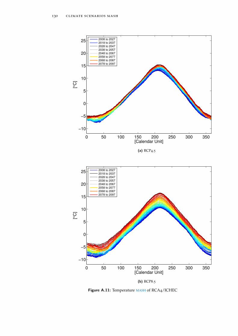
130 climate scenarios mash
0 50 100 150 200 250 300 350
−10
−5
0
5
10
15
20
25
[Calendar Unit]
[°C
]
2008 to 2027
2018 to 2037
2028 to 2047
2038 to 2057
2048 to 2067
2058 to 2077
2068 to 2087
2078 to 2097
(a) RCP4.5
0 50 100 150 200 250 300 350
−10
−5
0
5
10
15
20
25
[Calendar Unit]
[°C
]
2008 to 2027
2018 to 2037
2028 to 2047
2038 to 2057
2048 to 2067
2058 to 2077
2068 to 2087
2078 to 2097
(b) RCP8.5
Figure A.11: Temperature MASH of RCA4/ICHEC

climate scenarios mash 131
0 50 100 150 200 250 300 350
2
3
4
5
6
7
8
9
Calendar Unit
[mm
/da
y]
2008 to 2027
2018 to 2037
2028 to 2047
2038 to 2057
2048 to 2067
2058 to 2077
2068 to 2087
2078 to 2097
(a) RCP4.5
0 50 100 150 200 250 300 350
2
3
4
5
6
7
8
9
Calendar Unit
[mm
/da
y]
2008 to 2027
2018 to 2037
2028 to 2047
2038 to 2057
2048 to 2067
2058 to 2077
2068 to 2087
2078 to 2097
(b) RCP8.5
Figure A.12: Precipitation MASH of RCA4/ICHEC

132 climate scenarios mash
0 50 100 150 200 250 300 350
−10
−5
0
5
10
15
20
25
[Calendar Unit]
[°C
]
2008 to 2027
2018 to 2037
2028 to 2047
2038 to 2057
2048 to 2067
2058 to 2077
2068 to 2087
2078 to 2097
(a) RCP4.5
0 50 100 150 200 250 300 350
−10
−5
0
5
10
15
20
25
[Calendar Unit]
[°C
]
2008 to 2027
2018 to 2037
2028 to 2047
2038 to 2057
2048 to 2067
2058 to 2077
2068 to 2087
2078 to 2097
(b) RCP8.5
Figure A.13: Temperature MASH of HIRHAM/ICHEC

climate scenarios mash 133
0 50 100 150 200 250 300 350
2
3
4
5
6
7
8
9
Calendar Unit
[mm
/da
y]
2008 to 2027
2018 to 2037
2028 to 2047
2038 to 2057
2048 to 2067
2058 to 2077
2068 to 2087
2078 to 2097
(a) RCP4.5
0 50 100 150 200 250 300 350
2
3
4
5
6
7
8
9
Calendar Unit
[mm
/da
y]
2008 to 2027
2018 to 2037
2028 to 2047
2038 to 2057
2048 to 2067
2058 to 2077
2068 to 2087
2078 to 2097
(b) RCP8.5
Figure A.14: Precipitation MASH of HIRAM/ICHEC

134 climate scenarios mash
0 50 100 150 200 250 300 350
−10
−5
0
5
10
15
20
25
[Calendar Unit]
[°C
]
2008 to 2027
2018 to 2037
2028 to 2047
2038 to 2057
2048 to 2067
2058 to 2077
2068 to 2087
2078 to 2097
(a) RCP4.5
0 50 100 150 200 250 300 350
−10
−5
0
5
10
15
20
25
[Calendar Unit]
[°C
]
2008 to 2027
2018 to 2037
2028 to 2047
2038 to 2057
2048 to 2067
2058 to 2077
2068 to 2087
2078 to 2097
(b) RCP8.5
Figure A.15: Temperature MASH of CCLM/ICHEC
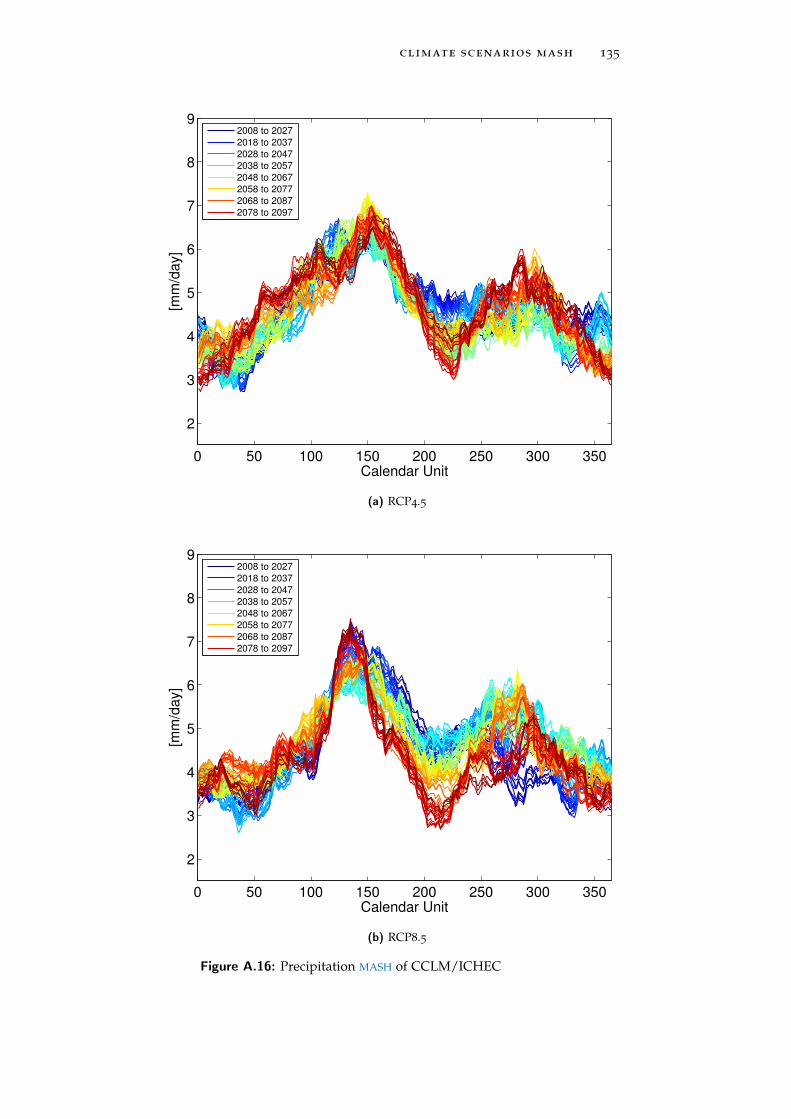
climate scenarios mash 135
0 50 100 150 200 250 300 350
2
3
4
5
6
7
8
9
Calendar Unit
[mm
/da
y]
2008 to 2027
2018 to 2037
2028 to 2047
2038 to 2057
2048 to 2067
2058 to 2077
2068 to 2087
2078 to 2097
(a) RCP4.5
0 50 100 150 200 250 300 350
2
3
4
5
6
7
8
9
Calendar Unit
[mm
/da
y]
2008 to 2027
2018 to 2037
2028 to 2047
2038 to 2057
2048 to 2067
2058 to 2077
2068 to 2087
2078 to 2097
(b) RCP8.5
Figure A.16: Precipitation MASH of CCLM/ICHEC

136 climate scenarios mash
0 50 100 150 200 250 300 350
−10
−5
0
5
10
15
20
25
[Calendar Unit]
[°C
]
2008 to 2027
2018 to 2037
2028 to 2047
2038 to 2057
2048 to 2067
2058 to 2077
2068 to 2087
2078 to 2097
(a) RCP4.5
0 50 100 150 200 250 300 350
−10
−5
0
5
10
15
20
25
[Calendar Unit]
[°C
]
2008 to 2027
2018 to 2037
2028 to 2047
2038 to 2057
2048 to 2067
2058 to 2077
2068 to 2087
2078 to 2097
(b) RCP8.5
Figure A.17: Temperature MASH of CCLM/MPI

climate scenarios mash 137
0 50 100 150 200 250 300 350
2
3
4
5
6
7
8
9
Calendar Unit
[mm
/da
y]
2008 to 2027
2018 to 2037
2028 to 2047
2038 to 2057
2048 to 2067
2058 to 2077
2068 to 2087
2078 to 2097
(a) RCP4.5
0 50 100 150 200 250 300 350
2
3
4
5
6
7
8
9
Calendar Unit
[mm
/da
y]
2008 to 2027
2018 to 2037
2028 to 2047
2038 to 2057
2048 to 2067
2058 to 2077
2068 to 2087
2078 to 2097
(b) RCP8.5
Figure A.18: Precipitation MASH of CCLM/MPI


BH Y D R O L O G I C A L S C E N A R I O S M A S H
139

140 hydrological scenarios mash
0 50 100 150 200 250 300 3500
50
100
150
200
250
Calendar Unit
[m3/s
]
2008 to 2027
2018 to 2037
2028 to 2047
2038 to 2057
2048 to 2067
2058 to 2077
2068 to 2087
2078 to 2097
(a) RCP4.5
0 50 100 150 200 250 300 3500
50
100
150
200
250
Calendar Unit
[m3/s
]
2008 to 2027
2018 to 2037
2028 to 2047
2038 to 2057
2048 to 2067
2058 to 2077
2068 to 2087
2078 to 2097
(b) RCP8.5
Figure B.1: RCA4/MIROC, Fuentes streamflow

hydrological scenarios mash 141
0 50 100 150 200 250 300 3500
50
100
150
200
250
Calendar Unit
[m3/s
]
2008 to 2027
2018 to 2037
2028 to 2047
2038 to 2057
2048 to 2067
2058 to 2077
2068 to 2087
2078 to 2097
(a) RCP4.5
0 50 100 150 200 250 300 3500
50
100
150
200
250
Calendar Unit
[m3/s
]
2008 to 2027
2018 to 2037
2028 to 2047
2038 to 2057
2048 to 2067
2058 to 2077
2068 to 2087
2078 to 2097
(b) RCP8.5
Figure B.2: RCA4/NCC, Fuentes streamflow

142 hydrological scenarios mash
0 50 100 150 200 250 300 3500
50
100
150
200
250
Calendar Unit
[m3/s
]
2008 to 2027
2018 to 2037
2028 to 2047
2038 to 2057
2048 to 2067
2058 to 2077
2068 to 2087
2078 to 2097
(a) RCP4.5
0 50 100 150 200 250 300 3500
50
100
150
200
250
Calendar Unit
[m3/s
]
2008 to 2027
2018 to 2037
2028 to 2047
2038 to 2057
2048 to 2067
2058 to 2077
2068 to 2087
2078 to 2097
(b) RCP8.5
Figure B.3: RCA4/NOAA, Fuentes streamflow

hydrological scenarios mash 143
0 50 100 150 200 250 300 3500
50
100
150
200
250
Calendar Unit
[m3/s
]
2008 to 2027
2018 to 2037
2028 to 2047
2038 to 2057
2048 to 2067
2058 to 2077
2068 to 2087
2078 to 2097
(a) RCP4.5
0 50 100 150 200 250 300 3500
50
100
150
200
250
Calendar Unit
[m3/s
]
2008 to 2027
2018 to 2037
2028 to 2047
2038 to 2057
2048 to 2067
2058 to 2077
2068 to 2087
2078 to 2097
(b) RCP8.5
Figure B.4: RCA4/CCC, Fuentes streamflow

144 hydrological scenarios mash
0 50 100 150 200 250 300 3500
50
100
150
200
250
Calendar Unit
[m3/s
]
2008 to 2027
2018 to 2037
2028 to 2047
2038 to 2057
2048 to 2067
2058 to 2077
2068 to 2087
2078 to 2097
(a) RCP4.5
0 50 100 150 200 250 300 3500
50
100
150
200
250
Calendar Unit
[m3/s
]
2008 to 2027
2018 to 2037
2028 to 2047
2038 to 2057
2048 to 2067
2058 to 2077
2068 to 2087
2078 to 2097
(b) RCP8.5
Figure B.5: RCA4/CNRM, Fuentes streamflow
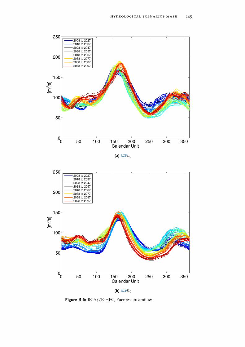
hydrological scenarios mash 145
0 50 100 150 200 250 300 3500
50
100
150
200
250
Calendar Unit
[m3/s
]
2008 to 2027
2018 to 2037
2028 to 2047
2038 to 2057
2048 to 2067
2058 to 2077
2068 to 2087
2078 to 2097
(a) RCP4.5
0 50 100 150 200 250 300 3500
50
100
150
200
250
Calendar Unit
[m3/s
]
2008 to 2027
2018 to 2037
2028 to 2047
2038 to 2057
2048 to 2067
2058 to 2077
2068 to 2087
2078 to 2097
(b) RCP8.5
Figure B.6: RCA4/ICHEC, Fuentes streamflow
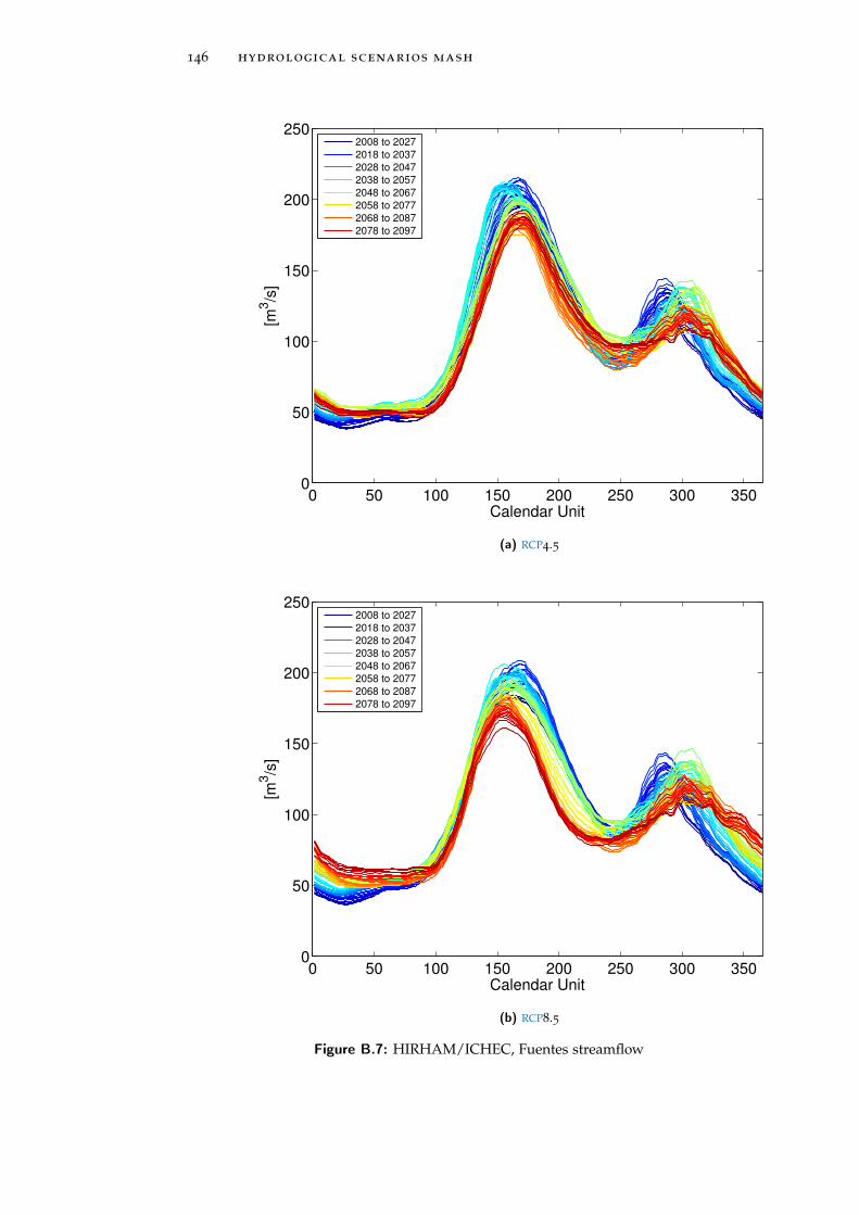
146 hydrological scenarios mash
0 50 100 150 200 250 300 3500
50
100
150
200
250
Calendar Unit
[m3/s
]
2008 to 2027
2018 to 2037
2028 to 2047
2038 to 2057
2048 to 2067
2058 to 2077
2068 to 2087
2078 to 2097
(a) RCP4.5
0 50 100 150 200 250 300 3500
50
100
150
200
250
Calendar Unit
[m3/s
]
2008 to 2027
2018 to 2037
2028 to 2047
2038 to 2057
2048 to 2067
2058 to 2077
2068 to 2087
2078 to 2097
(b) RCP8.5
Figure B.7: HIRHAM/ICHEC, Fuentes streamflow

hydrological scenarios mash 147
0 50 100 150 200 250 300 3500
50
100
150
200
250
Calendar Unit
[m3/s
]
2008 to 2027
2018 to 2037
2028 to 2047
2038 to 2057
2048 to 2067
2058 to 2077
2068 to 2087
2078 to 2097
(a) RCP4.5
0 50 100 150 200 250 300 3500
50
100
150
200
250
Calendar Unit
[m3/s
]
2008 to 2027
2018 to 2037
2028 to 2047
2038 to 2057
2048 to 2067
2058 to 2077
2068 to 2087
2078 to 2097
(b) RCP8.5
Figure B.8: CCLM/ICHEC, Fuentes streamflow

148 hydrological scenarios mash
0 50 100 150 200 250 300 3500
50
100
150
200
250
Calendar Unit
[m3/s
]
2008 to 2027
2018 to 2037
2028 to 2047
2038 to 2057
2048 to 2067
2058 to 2077
2068 to 2087
2078 to 2097
(a) RCP4.5
0 50 100 150 200 250 300 3500
50
100
150
200
250
Calendar Unit
[m3/s
]
2008 to 2027
2018 to 2037
2028 to 2047
2038 to 2057
2048 to 2067
2058 to 2077
2068 to 2087
2078 to 2097
(b) RCP8.5
Figure B.9: CCLM/MPI, Fuentes streamflow