WATER RESOURCE SUSTAINABILITY OF THE PALOUSE REGION: A SYSTEMS APPROACH

WATER RESOURCE SUSTAINABILITY OF THE PALOUSE REGION: A

SYSTEMS APPROACH

A Thesis

Presented in Partial Fulfillment of the Requirements for the

Degree of Master of Science

With a

Major in Civil Engineering

In the College of Graduate Studies

University of Idaho

by:

Ramesh Dhungel

December 2007

Major Professor: Fritz Fiedler, Ph.D., P.E.

ii

AUTHORIZATION TO SUBMIT THESIS

This thesis of Ramesh Dhungel, submitted for the degree of Master of Science with a major

in Civil Engineering and titled “Water Resource Sustainability of the Palouse Region: A

Systems Approach” has been reviewed in final form. Permission, as indicated by the

signatures and dates given below, is now granted to submit final copies to the College of

Graduate Studies for approval.

Major Professor Date Fritz Fiedler Committee Members Date

Chuck Harris

Date Erik R. Coats Department Administrator Date Sunil Sharma

Discipline’s College Dean Date Aicha Elshabini

Final Approval and Acceptance by the College of Graduate Studies

Date Margrit von Braun

iii

Abstract

The system dynamics approach was utilized for evaluating the sustainability of water

resources of the Palouse Region. The Palouse Basin, located on the border of Idaho and

Washington states, has three cities: Moscow, Pullman and Colfax. Water demand is

completely fulfilled by the groundwater aquifers. Two confined groundwater aquifers

systems exist, the upper Wanapum, and the lower Grande Ronde. These aquifers are located

within the basaltic Columbia River flows. The water levels of the Grande Ronde have been

declining up to 2 feet each year for more than fifty years. Study of these aquifers indicates

that there is likely to be a close relation between groundwater pumping and groundwater

depletion. This research was conducted to provide a broad synthesis of existing water

resources data, to understand the long-term implications of continued growth and water

demand on basin water resources, and to move towards sustainable management.

Demographic, hydrologic, geologic and economic data were collected and used to

develop systems models, comprised of population, hydrological and economical modules.

Water demand was forecasted by the population and demand components. Exponential

population growth was simulated with 1% annual growth for the entire Palouse Basin. The

hydrological component has groundwater and surface elements. In the Simple Model (SM),

groundwater of all regions was lumped into a single unit. In the Hydraulically Separated

Model (HSM), groundwater was divided into geological regions. A water balance at the land

surface was used to estimate recharge to the Wanapum. Leakage between the Wanapum and

Grande Ronde is allowed, and a range of recharge rates to the Grande Ronde is taken from

previously published estimates. A groundwater- surface water overlay was created to help

estimate recharge.

iv

Log-linear regression was used to find the relationship between the water demand and

several independent variables. Price elasticity of water demand of City of Pullman was

calculated. An economic module was developed from the regression equation with linear

extrapolation of the independent variables. Water demand was projected from the economic

module developed from the regression equation.

The water balance resulted in a mean areal precipitation of 71 centimeters,

evapotranspiration of 49 centimeters, runoff of 17 centimeters and recharge of 4.7

centimeters. The recharge from the water balance indicated a water level increase in the

Wanapum aquifer. The life of the aquifers depends on the initial volume of the aquifer and

recharge to the aquifer. The initial volume of the Grande Ronde is approximately 43 billion

gallons, and 1.6 billion gallons in the Wanapum, based on a storativity value of 10-3. Under

the current conditions, the SM projected the life of the Wanapum to be more than 100 years,

while the Grande Ronde life ranged from a couple of years to more than 100 years. Using the

current infrastructure and published storativity values (10-3 to 10-5), with no recharge

assumed to the Grande Ronde, the life of the Grande Ronde is simulated to be less than 20

years. Assuming one centimeter of recharge to the Grande Ronde added 30 years, and

assuming two centimeters added 100 years. The storativity was back-calculated with current

water extraction and water level decline rates to be 0.03. The back-calculated storativity

added 100 years to the life of the Grande Ronde. Because of the modeled hydraulic

separation among the groundwater regions, the HSM projects a comparatively shorter life of

the Moscow and Pullman Grande Ronde. So, if actual hydrological separation exists between

the groundwater regions, such separation may significantly affect water management of the

Palouse Basin.

v

To consider future water resources development, it was assumed that 80% of the

surface water can be potentially utilized. Paradise Creek was used for fulfilling Moscow’s

water demand, and the South Fork Palouse River for Pullman. In this applied water

management strategy, the surface water is able to fulfill water demand for the coming 100

years.

Regression results showed the price elasticity of water demand of marginal price is

inelastic while fixed price is elastic. The price elasticity of marginal price ranges from +1.6

to +2.97, indicating inelasticity. The exponents for median household income, fixed price and

precipitation had the expected signs in the regression equation. The developed economic

module projected a decline in water demand when the independent variables are assumed to

grow linearly over the coming 25 years.

A Sustainability Index showed that the Wanapum water use to be sustainable given

the present water use trend and infrastructure, while the Grande Ronde use was predicted to

be unsustainable.

vi

Acknowledgement

I would like to acknowledge my advisor Dr. Fritz Fiedler for his generous support.

This work would not have been possible with out his help and guidance. I am thankful to

Water of West (WOW) for the fund. I would like to thank Professor Chuck Harris and Dr.

Erik Coats for their continuous support and critical review of this thesis. I also want to thank

Dr. Erin Brooks, Professor John Bush, Dr. Ashley Lyman and Ms. Jennifer Hinds for helping

me understand different subject matters. I am thankful to all the staff and faculty member of

Department of Civil Engineering, Department of Statistics and writing center at University of

Idaho for their help to the completion of this thesis. I would like to thank City of Pullman,

City of Moscow and Washington State University for providing me supporting data for this

thesis.

I am grateful to my entire family member, specially my father and mother for their

support and inspiration, sister Rama and her husband Kailash, Rachana and her husband

Bikash, and my brother Ranjan for their help. Last but not the least, I am thankful to

colleagues, friends and the Nepalese community in Moscow that makes me feel home away

from home.

vii

Dedication

This thesis is dedicated to my parents Chandra Raj and Geeta

viii

Table of Contents

AUTHORIZATION TO SUBMIT THESIS............................................................................. ii

Abstract .................................................................................................................................... iii

Acknowledgement ................................................................................................................... vi

Dedication ............................................................................................................................... vii

Table of Contents................................................................................................................... viii

List of Figures .......................................................................................................................... xi

List of Tables .........................................................................................................................xiii

CHAPTER I .............................................................................................................................. 1

INTRODUCTION ................................................................................................................ 1

1.0 Overview..................................................................................................................... 1

1.1 Water Resource Management ..................................................................................... 1

1.2 Overview of Study Area ............................................................................................. 2

1.3 Palouse Basin Management ........................................................................................ 7

1.4 Background ............................................................................................................... 10

1.5 Objectives ................................................................................................................. 13

CHAPTER II........................................................................................................................... 14

LITERATURE REVIEW ................................................................................................... 14

2.0 Overview................................................................................................................... 14

2.1 Water Resource Sustainability.................................................................................. 14

2.2 Water Balance Approach to Recharge...................................................................... 17

2.3 Previous Study of Recharge of the Palouse Basin .................................................... 19

2.4 Water Pricing and Price Elasticity of Demand ......................................................... 21

2.5 System Dynamics Approach..................................................................................... 23

CHAPTER III ......................................................................................................................... 27

DATA REQUIRED FOR MODELING ............................................................................. 27

3.0 Overview................................................................................................................... 27

3.1 Watershed Map and Area.......................................................................................... 27

3.2 Geology of Palouse Basin Aquifer ........................................................................... 28

3.3 Aquifer Volume ........................................................................................................ 32

3.4 Precipitation Data for Hydrologic Model ................................................................. 35

3.5 Surface Runoff .......................................................................................................... 36

3.6 Evapotranspiration (ET)............................................................................................ 37

3.7 Recharge to Wanapum.............................................................................................. 38

3.8 Recharge to Grande Ronde ....................................................................................... 39

ix

3.9 Water Demand and Per Capita Water Use................................................................ 40

3.10 Population and Growth Data................................................................................... 40

3.11 Economic Data........................................................................................................ 41

CHAPTER IV ......................................................................................................................... 46

MODEL DEVELOPMENT SCENARIOS......................................................................... 46

4.0 Overview................................................................................................................... 46

4.1 Interactions among the Models................................................................................. 46

4.2 Population and Demand Forecast Model.................................................................. 48

4.3 Hydrological Model .................................................................................................. 49

4.4 Economic Module..................................................................................................... 58

4.5 Water Management Strategy..................................................................................... 61

4.6 Sustainability Index (SI) ........................................................................................... 65

CHAPTER V .......................................................................................................................... 67

RESULTS AND DISCUSSION......................................................................................... 67

5.0 Overview................................................................................................................... 67

5.1 Domestic Water Demand.......................................................................................... 67

5.2 Simple Model (SM) .................................................................................................. 69

5.3 Hydrologically Separated Model (HSM).................................................................. 88

5.4 HSM for Water Resource Management with Current Infrastructures ...................... 93

5.5 HSM with Simple Economics................................................................................... 94

5.6 HSM with Surface Water.......................................................................................... 97

5.7 Surface Water.......................................................................................................... 106

5.8 Sustainability Index (SI) ......................................................................................... 108

5.9 Summary................................................................................................................. 110

CHAPTER VI ....................................................................................................................... 112

CONCLUSIONS............................................................................................................... 112

6.0 Overview................................................................................................................. 112

6.1 System Dynamics Approach................................................................................... 112

6.2 SM and HSM .......................................................................................................... 113

6.3 Wanapum and Grande Ronde ................................................................................. 113

6.4 Watershed Economics............................................................................................. 115

6.5 Sustainability of Aquifers ....................................................................................... 115

6.6 Calibration and Validations .................................................................................... 116

6.7 Data and Results Quality ........................................................................................ 117

6.8 Summary................................................................................................................. 118

6.9 Recommendations................................................................................................... 118

x

6.10 Limitations ............................................................................................................ 122

REFERENCES ..................................................................................................................... 123

APPENDIX A....................................................................................................................... 129

Water Extraction Data of Four entities (1964-2005) ........................................................ 129

APPENDIX B ....................................................................................................................... 131

Comprehensive Data Set of City of Pullman for Economic Analysis .............................. 131

APPENDIX C ....................................................................................................................... 134

Model Development Sections in STELLA Software........................................................ 134

APPENDIX D....................................................................................................................... 156

Equations in Stella ............................................................................................................ 156

APPENDIX E ................................................................................................................... 170

3D Projection of Palouse Basin Groundwater Surface Water Overlay ............................ 170

xi

List of Figures

Figure 1-1: Palouse Basin Watershed...................................................................................... 3

Figure 1-2: North Fork and South Fork Palouse River............................................................ 4

Figure 1-3: Groundwater Basin with Six Regions (Bush and Hinds, 2006)............................ 5

Figure 1-4: Water Extraction from Four Entities..................................................................... 7

Figure 1-5: Composite Hydrograph of Wells in the Palouse Basin....................................... 11

Figure 1-6: Water Level Fluctuation in Moscow Grande Ronde .......................................... 12

Figure 1-7: Water Level Fluctuation in Pullman Grande Ronde........................................... 12

Figure 2-1: Major Considerations in Water Resource Management ..................................... 15

Figure 2-2: Water Resources Balance (Miloradov, 1995)..................................................... 18

Figure 2-3: Components of STELLA Software..................................................................... 25

Figure 3-1: Schematic East West Cross Section of Study Area (Owsley, 2003) .................. 31

Figure 3-2: Definition Sketch for Calculating Volume of Water in the Aquifers ................. 33

Figure 3-3: Water Consumption and Marginal Price............................................................. 43

Figure 3-4: Monthly Water Consumption of Residential Sector of City of Pullman............ 44

Figure 4-1: Interaction between the Models .......................................................................... 47

Figure 4-2: Population Model................................................................................................ 48

Figure 4-3: Groundwater- Surface Water Overlay ................................................................ 50

Figure 4-4: Schematic of SM of the Palouse Basin ............................................................... 52

Figure 4-5: Schematic of Connectivity in the HSM .............................................................. 54

Figure 5-1: Water Demand Projection of the Palouse Basin ................................................. 68

Figure 5-2: Water Demand Projection of the Major Cities ................................................... 68

Figure 5-3: SM-1 ................................................................................................................... 71

Figure 5-4: SM-2 ................................................................................................................... 72

Figure 5-5: SM-3 ................................................................................................................... 72

Figure 5-6: SM-4 ................................................................................................................... 73

Figure 5-7: SM-5 ................................................................................................................... 74

Figure 5-8: SM-5 (Feet)......................................................................................................... 74

Figure 5-9: SM-6 ................................................................................................................... 75

Figure 5-10: SM-7 ................................................................................................................. 76

Figure 5-11: SM-8 ................................................................................................................. 77

Figure 5-12: SM-8 (Feet)....................................................................................................... 78

Figure 5-13: SM-9 ................................................................................................................. 79

Figure 5-14: SM-10 ............................................................................................................... 80

Figure 5-15: SM-10 (Feet)..................................................................................................... 80

xii

Figure 5-16: SM-11 ............................................................................................................... 82

Figure 5-17: SM-12 ............................................................................................................... 82

Figure 5-18: SM-13 ............................................................................................................... 83

Figure 5-19: SM-13 (Feet)..................................................................................................... 84

Figure 5-20: Wanapum Water Level Trend (Ralston, 2004)................................................. 85

Figure 5-21: HSM-1............................................................................................................... 89

Figure 5-22: HSM-2............................................................................................................... 89

Figure 5-23: HSM-2 (Palouse, Colfax and Viola)................................................................. 90

Figure 5-24: HSM-3............................................................................................................... 91

Figure 5-25: HSM-5............................................................................................................... 93

Figure 5-26: Moscow water management without surface water (HSM-4) .......................... 94

Figure 5-27: Linear Extrapolation of Independent variables for Regression Equation......... 95

Figure 5-28: Water Demand Projection by Economic Module ............................................. 96

Figure 5-29: Water Extraction Pattern of Moscow (HSM-3) ................................................ 98

Figure 5-30: Groundwater Volume in Moscow Region Aquifers (HSM-3) ......................... 99

Figure 5-31: Water Extraction Pattern of Moscow (HSM-4) .............................................. 100

Figure 5-32: Groundwater Volume in Moscow Region Aquifers (HSM-4) ....................... 101

Figure 5-33: Water Extraction Pattern of Pullman (HSM-2) .............................................. 102

Figure 5-34: Groundwater Volume in Pullman Region Aquifers (HSM-2)........................ 103

Figure 5-35: Water Extraction Pattern of Pullman (HSM-4) .............................................. 104

Figure 5-36: Groundwater Volume in Pullman Region Aquifers (HSM-4)........................ 105

Figure 5-37: South Fork Palouse River Sub-Basins ............................................................ 107

Figure 5-38: SI Grande Ronde (HSM-6) ............................................................................. 109

Figure 5-39: SI Wanapum (SM-4)....................................................................................... 110

Figure 6-1: Future Schematic of SM of the Palouse Basin.................................................. 120

xiii

List of Tables

Table 2-1: Estimated Recharge Rates (WRIA-34) ................................................................ 20

Table 3-1: Area of Sub-Watersheds....................................................................................... 28

Table 3-2: Aquifer Volume, Area and Thickness (Bush and Hinds, 2006)........................... 30

Table 3-3: Potential Groundwater Drawdown (PBAC, 1999)............................................... 34

Table 3-4: Surface Area of Wanapum and Grand Ronde Basalts (Bush and Hinds, 2006) .. 35

Table 3-5: Mean Areal Precipitation of Palouse Basin Sub-Watersheds .............................. 36

Table 3-6: Period of Availability of Daily Discharge of USGS Gauging Stations................ 36

Table 3-7: Mean Areal Surface Runoff of Palouse Basin Sub-Watersheds .......................... 37

Table 3-8: Mean Areal Evapotranspiration of Palouse Basin Sub-Watersheds..................... 38

Table 3-9: Mean Areal Recharge of Palouse Basin Sub-Watersheds.................................... 39

Table 3-10: Population of major cities................................................................................... 40

Table 3-11: Marginal and Fixed Price Rates of City of Pullman........................................... 42

Table 3-12: Sample Data for Economic Analysis of Single Family, Pullman, Washington . 45

Table 4-1: Components of Water Balance of SM.................................................................. 53

Table 4-2: Components of Water Balance of HSM............................................................... 56

Table 4-3: Initial Volume of Groundwater in Aquifers ......................................................... 57

Table 4-4: Annual Recharge to the Designated Wanapum Groundwater Regions................ 58

Table 4-5: Regression Coefficients for Price Elasticity Curve for Single Family................. 59

Table 4-6: Regression Coefficients for Price Elasticity Curve for Residential Households . 60

Table 5-1 : SM Applied Conditions....................................................................................... 70

Table 5-2: Summary Table of the Life of the Groundwater Aquifers ................................... 86

Table 5-3: Projection of Present Water Level Depletion Trend ............................................ 87

Table 5-4: HSM for Water Management ............................................................................... 88

Table 5-5: Summary of Management Strategies.................................................................... 97

Table 5-6: Summary Table of Life of the Groundwater Aquifers ....................................... 105

Table 5-7: Summary of Paradise Creek and South Fork Palouse at Pullman...................... 108

Table 5-8: Estimated Surface Water Availability (Stasney, 2006)...................................... 108

1

CHAPTER I

INTRODUCTION

1.0 Overview

This chapter briefly discusses the general concept of water resources management

including the current water resource scenario of the Palouse Basin. The Palouse Basin, a

semi-arid area located along the border of northern Idaho and eastern Washington, is solely

dependent on groundwater for drinking water. The depletion of groundwater in the aquifers is

the major concern of this Basin. The background of this research is to analyze the water level

depletion of these aquifers, study the water use practice and recommend some future steps

for efficient water resource management. The major objective of this study is to use System

Dynamics Approach for evaluating and managing water resources of this basin.

1.1 Water Resource Management

Water resources can be managed primarily as surface water or groundwater or both

according to the geographic location and availability of water. In the United States, 74

percent of total public supply is provided by surface water during 1950 and 63 percent at

2000 with 11 percent decrease (Hutson et al., 2000). In comparison, 96 percent is fulfilled by

groundwater sources in Idaho (Anderson and Woosley, 2002). This indicates the increasing

trend of groundwater use in the public supply. Due to its widespread occurrence, generally

good quality and high reliability during droughts, the use of groundwater has increased

significantly in recent decades (Vrba and Lipponen, 2007). Because of scarcity and the

temporal unreliability of surface water resources in arid and semi-arid regions, the primary

source of drinking water is usually groundwater (Scanlon et al., 2006). But according to the

International Atomic Energy Agency (IAEA), much of the groundwater extracted in semi-

2

arid areas is “fossil water” (not recently recharged) and its use is not sustainable (Scanlon et

al., 2006). The combined utilization of surface water and groundwater can improve water

resources management in semi-arid regions.

For effective water resources management, it is necessary to understand the

interaction between groundwater and surface water. Efficient and sustainable management of

groundwater resources requires quantifying groundwater recharge (Khazaei et al., 2003).

Groundwater recharge can be broadly defined as the addition of water to a groundwater

reservoir (Vrba and Lipponen, 2007). In semi-arid areas, the variation of groundwater

recharge is typically significant in both space and time (Khazaei et al., 2003). Water tables

are often deep with localized (focused) recharge in semi-arid and arid areas, and there are

various mechanisms of recharge, such as infiltration from the beds of ephemeral streams, and

subsurface drainage from mountain areas through the alluvial material of valley beds

(Khazaei et al., 2003).

Due to the complexities of geologic formations and uncertainties in parameters such

as storativity (described subsequently), characterization of groundwater aquifers is

challenging. The most difficult component of the hydrologic budget is to quantify

groundwater recharge (Khazaei et al., 2003). So, the importance of recharge in the water

resources management is clear especially where groundwater is the major source of drinking

water. At this point, the important question is the estimation of the inflow, outflow and the

amount of stored water in an aquifer in particular spatial and temporal dimension.

1.2 Overview of Study Area

The Palouse Basin spans eastern Washington and northern Idaho. The major portion

is within Whitman County of Washington State, and Latah County of Idaho state, with a very

3

small area in Benewah County in Idaho. Figure 1-1 shows the Palouse Basin divided into six

sub-basins defined by United State Geological Survey (USGS) surface water gauging station

locations and state boundary (straight line at bottom).

Figure 1-1: Palouse Basin Watershed

The total area of the delineated watershed in this study is approximately 2,044 square

kilometers (km2). The largest cities within the watershed are Pullman, Moscow and Colfax

while other smaller towns are Palouse, Princeton, Viola, Potlatch, Onaway, and Harvard. The

4

Palouse Region is a semi-arid area where precipitation ranges from approximately 59 to 85

centimeters per year (yr). With elevation increasing to the east, the precipitation of Palouse

Basin increases. The mean temperature of the Palouse Basin decreases from west to east. The

precipitation of the Palouse Basin is either in the form of rain or snowfall. The North Fork

Palouse River and the South Fork Palouse River are major rivers of this basin (Figure 1-2).

The sub-watersheds delineated from the South Fork Palouse River can be termed as South

Fork Palouse Basin Watershed and North Fork Palouse Basin Watershed from the North

Fork Palouse River. Paradise Creek, Missouri Flat Creek and Fourmile Creek are some other

streams in the watershed. The runoff in these rivers is influenced by the snow melting and

rainfall in the frozen ground in the spring seasons (Palouse Basin Community Information

System, 2007).

Figure 1-2: North Fork and South Fork Palouse River

(Source: Palouse Basin Community Information System, 2007)

According to the geographic variations, the groundwater regions are divided into

Palouse, Colfax, Viola, Pullman, Moscow and Uniontown regions (Figure 1-3). The

5

uppermost layer of the Palouse Basin is composed of loess which is basically a deposit of

wind-blown silt. According to the dominant geologic formations, there are two groundwater

aquifers in the Palouse Basin, identified as the Wanapum (WP) and Grande Ronde aquifers

(GR). The composition of these aquifers is more than 60 percent basalt, with the rest being

sediments including silt, clay and sand. Both Wanapum and Grande Ronde are confined

aquifers (Larson et al., 2000).

Figure 1-3: Groundwater Basin with Six Regions (Bush and Hinds, 2006)

6

The Wanapum aquifer is the shallower of the two at approximately 110m deep and

the Grande Ronde aquifer at approximately 290m. These thicknesses (depth) represent the

potential depth of water extraction in these confined aquifers. The “2000 Annual Report

Water Use in the Palouse Basin” reports that water levels of these aquifers have been

decreasing up to 2 feet annually (McKenna, 2001) for seventy years (Robinschon, 2006,

PBAC, 2006). By 1923, the water level of the Wanapum aquifer had dropped to

approximately 13.4 meters below the surface and about 30.5 meters below the surface water

by 1957(Bloomberg, 1959).

The shallower Wanapum aquifer is the primary water supply for rural residents of

Latah County within the basin limits and in some areas of Whitman County (McKenna,

2001) and supplies approximately 32 percent Moscow’s drinking water (Ralston, 2004,

PBAC, 2006). Approximately 70 percent of Moscow’s and 100 percent of Pullman’s

drinking water demand is fulfilled by the lower Grande Ronde aquifer. These aquifers have

satisfactory groundwater quality for domestic, agricultural and industrial purposes. Also,

these aquifers have been the subject of much research over the last 40 years.

The total population of the area is about 51,000 people. The population within 7 miles

of Moscow and Pullman is denser compared to rest of the regions (i.e., Colfax, Viola and

Palouse). The decreasing level of groundwater in these aquifers, and thus its sustainability, is

a major concern of basin residents. If we review the water use pattern of the City of Moscow,

in 1964, 560 million gallons of water was extracted from City of Moscow pumping stations

and 820 millions gallons in 2005, a 46 percent rise. Figure 1-4 shows the trend of water use

by four major entities (i.e., City of Pullman, City of Moscow, University of Idaho and

Washington State University) from 1964 to 2005 (Appendix A).

7

0

200

400

600

800

1000

1960 1970 1980 1990 2000

Years

Wa

ter

Ex

tra

ctio

n (

Mil

lio

n G

all

on

s)Pullman

Washington

State University

University of

Idaho

Moscow

Figure 1-4: Water Extraction from Four Entities

1.3 Palouse Basin Management

Several organizations and social groups have been working in this basin for some

time. Among them are the Palouse Basin Aquifer Committee (PBAC), Palouse Conservation

District, the Palouse Water Conservation Network and Protect Our Water. All essentially

have the common goal of sustainable use for water in the aquifer. Few studies are carried out

about the surface water utilization of this Basin. A feasibility study was carried by Stevens,

Thompson, and Runyan in 1969 for utilizing surface water for the drinking water supply in

Pullman-Moscow area (McKenna, 1999). The study suggested construction of a pipeline

from the Palouse River at Laird Part in Latah County, or from the Snake River at Wawawai

County Park in Whitman (Stevens et al., 1970). At present, the use of surface water as an

additional supply is getting attention because of the threat of the groundwater scarcity in this

region.

The PBAC was formed in the late 1960s to address declining water levels in the

regional aquifers. It is a voluntary, cooperative, multi-jurisdictional committee comprised of

8

representatives from seven entities: University of Idaho (UI), Washington State University

(WSU), Pullman (Washington), Colfax (Washington), Moscow (Idaho), Whitman County

(Washington), and Latah County (Idaho). PBAC is guided by an intergovernmental

agreement signed by the stakeholder representatives. The Washington Department of

Ecology (WDOE) and the Idaho Department of Water Resources (IDWR) also have signed

an agreement with the committee. The purpose of the PBAC is to provide a forum for

stakeholders to address resource issues in the watershed, particularly by supporting research

to clarify the current situation of water resources in the basin and by considering possible

actions that members could take.

The management of the Palouse Basin was initiated in the 1960s. A significant effort

has been devoted to accelerate effective planning in the 1990s by implementing a Plan of

Action by PBAC. The major goal of the Plan of Action was to use the groundwater without

depleting the basin aquifers and protecting quality of water (PBAC, 1992). This Plan of

Action was the beginning action plan of all stakeholders of PBAC for the management of

groundwater with an attempt to limit the annual aquifer pumping that increases to one

percent of the pumping volume based on a five year moving average starting in 1986 (PBAC,

1992). The current stated mission of PBAC is to provide a long term, quality water supply

for the Palouse Basin by balancing basin wide water supply by 2020 (PBAC, 2006). PBAC

has developed a 20-Year Plan of the management of aquifer adopted in 2000 which is an

attempt to stabilize the declining groundwater levels in the deep Grande Ronde aquifer by the

year 2020. Furthermore; an important goal for achieving the above mission is to develop an

alternate water supply plan by 2010.

Water Resource Inventory Area (WRIA) 34 planning unit is composed of local and

9

state organizations of Washington and includes the state of Idaho as a voting member. Latah

County, Idaho, is included in the WRIA planning unit. Washington State watershed planning

process includes the following four phases. The first phase is an organization, second

assessment, third planning and final implementation. The Phase II level 1 is the phase of

compilation and reviewing of the existing data of the watershed. Level 2 of the Phase II is the

phase of collecting new data and level 3 is the long term monitoring of selected parameters

for improving management strategy. The planning phase should maintain the coordination

process, divide responsibilities, regulate and figure out funding sources. The planning phase

also provides the base for the implementation phase for managing water resources. It should

address the water resources management issues of agriculture, commercial, industrial and

residential sector including stream flow water.

The “Phase II-Level 1 Technical Assessment for the Palouse the Basin, Water

Resource Inventory Area (WRIA-34)” is an important study to address the management

aspect of the watershed that was prepared for the Palouse Planning Unit. Technical

requirements of the Watershed Planning Act (RCW 90.82) are fulfilled by this study. RCW

90.82, signed by the twelve state agencies in Washington, supports local government, interest

groups and citizens to manage water resources in WRIA areas. The key issues defined by

WRIA-34 of the Palouse Basin are future water availability (including some water rights

issues), concerns about water level decline in the Grande Ronde aquifer in the Pullman-

Moscow area and water quality concerns. Another important issue is to maintain cross-state

coordination with Idaho.

10

1.4 Background

The historical and on-going decreasing water level in the aquifers, particularly in the

Grande Ronde, is the major concern in the Palouse Basin, as this indicates unsustainable use.

Figure 1-5 shows the composite hydrograph of different wells in the Wanapum and Grande

Ronde aquifers in the Palouse Basin. The top section is the Palouse loess followed by the

Wanapum aquifer and the Grande Ronde (Figure 1-5). Figures 1-6 and 1-7 show the water

level fluctuation patterns of the Moscow and Pullman Grande Ronde wells. The apparent

depletion of groundwater level has the potential to create a scarcity of high quality drinking

water. Fluctuations in groundwater level might not simply and solely be indicative of

groundwater recharge and extraction, however. The naturally occurring changes in climate

and anthropogenic activities can contribute to long term fluctuations in groundwater level

over periods of decades (Healy et al., 2002). Due to the temporal variability of

evapotraspiration, precipitation, and irrigation, seasonal fluctuations in groundwater levels

are common in many areas. Phenomena like rainfall, pumping, barometric-pressure

fluctuations create seasonal fluctuations in groundwater levels (Healy et al., 2002). In the

year 1990, the City of Moscow reduced its dependence on Grande Ronde. From then,

approximately 70 percent of water was extracted from the Grande Ronde and the rest from

the Wanapum. But Pullman still is solely dependent in the Pullman Grande Ronde and there

has been constant depletion of the water level in the aquifer up to now.

The gradual increase in population and infrastructure development in Palouse Region

likely will lead to a further increase in water demand. But the declining groundwater level

raises the possible scarcity of drinking water in Palouse Region. So, the people residing in

this area are compelled to study groundwater in these aquifers and manage in a sustainable

11

manner according to the future need. The dependence on groundwater may be reduced by

using surface water, or it may be possible to use groundwater in a sustainable manner. The

primary goal of this research is to develop a model that provides a framework to study

sustainability and management of water resources of the Palouse Basin, synthesizing

available information and data using the “System Dynamics Approach” described in section

2.5.

Figure 1-5: Composite Hydrograph of Wells in the Palouse Basin

(Source: Leek F., 2006)

Figure 1-5 shows the groundwater level trend of the aquifers from the year 1923 to

2003. Figure 1-6 shows the long term hydrographs of Moscow and University of Idaho (UI)

wells.

12

Figure 1-6: Water Level Fluctuation in Moscow Grande Ronde

Figure 1-7 shows the long term hydrograph of Pullman and Washington State

University (WSU) wells.

Figure 1-7: Water Level Fluctuation in Pullman Grande Ronde

(Source: Leek, Wu, Bush, Qiu and Keller, 2005)

13

Both figures (1-6 and 1-7) show the water level is depleting in the Grande Ronde

aquifer.

1.5 Objectives

The overarching goal of this research is to develop a systems model to study water

resources sustainability of the Palouse Basin. The major objectives of this study are:

1. To estimate the quantity of surface and groundwater resources of the Palouse Basin at

particular temporal and spatial scales using available data and common calculation

methods;

2. To develop a water balance using these estimates and a systems model to simulate the

balance;

3. To link the developed water balance with estimates of demand, using population

growth and simple economics using systems modeling;

4. To use the model to explore sustainability and select management approaches; and

5. To conduct limited sensitivity analyses of the model to select parameters and various

future water use scenarios in the Palouse Basin.

14

CHAPTER II

LITERATURE REVIEW

2.0 Overview

This chapter is a review of literature on topics related to the water resources

management. The beginning section of this chapter discusses the concept of water resource

sustainability and sustainability index (SI). As recharge is one of the important components

of groundwater, water balance approach for calculating recharge is discussed. Some earlier

studies about the recharge computation of the Palouse Basin are also tabulated. The

relationship between the price and water demand is discussed in the section of the price

elasticity of water demand. And finally, the System Dynamics Approach and its use in water

resource planning and management is described.

2.1 Water Resource Sustainability

Creating balance between water demand and available water resources can be broadly

defined as sustainable water resources management (Simonovic et al., 1997). One definition

of sustainability states that “Sustainable water resource systems are those designed and

managed to fully contribute to the objectives of the society, now and in the future, while

maintaining their ecological, environmental, and hydrological integrity” (ASCE, 1998). The

“non-excessive” use of surface water, “non-depletive” groundwater abstraction, and

“efficient” re-use of treated wastewater are considered to be sustainable practices (Xu et al.,

2002). The Sustainable Water Resource Roundtable (SWRR) defines water use sustainability

as the ratio of water withdrawn to renewable supply (SWRR, 2005). The major

considerations for sustainable water resource management can be seen in Figure 2-1. Water

resource management is not only about the technical aspects of water demand and supply.

15

Sustainable management includes environmental, legal, social, economical and hydrological

aspects of water resources.

Figure 2-1: Major Considerations in Water Resource Management

Portland Basin, similar to the Palouse Basin, located across the Columbia River into

Southern Washington and Northern Oregon is also dependent on the deep aquifers for

regional water supply. Regional aquifer management of the Portland Basin purposed induced

recharge to decrease aquifer drawdown and increase sustainability of long-term groundwater

use (Koreny and Terry, 2001). It is not always easy to quantify the term sustainability but

there are several techniques available, such as sustainability indexes (SI) and indicators. The

ratio of water deficit relative to the corresponding supply can be defined as SI (Xu et al.,

2002). A 2002 article by Xu et al. used the approach where demand greater than 80 percent

of potential water supply was (arbitrarily) classified as vulnerable on the SI. Equation 2-1

shows how Xu defined the SI when supply is greater than demand and vice versa.

Environmental

Hydrologic

Economic Social

Legal

16

{

≤

>−=

DS

DSSDSSI

,0

,/)( (2-1)

where, D is the water demand and S is the available water-supply, in any consistent units.

There are numerous groundwater resource sustainability indicators published by

UNESCO (Vrba and Lipponen, 2007) in the report titled “Groundwater Resources

Sustainability Indicators.” In the context of the Palouse Region, understanding these

groundwater indicators has particular importance. The Groundwater Sustainability Indicator

(GSI) and Groundwater Depletion Indicator (GDI) are discussed briefly. In semi-arid areas,

to calculate GSI (Equation 2-2), the average annual abstraction and recharge values should be

used (Vrba and Lipponen, 2007). Three different scenarios were developed according to

abstraction and recharge conditions.

%100*TGR

TGAGSI = (2-2)

where, TGA is the total groundwater abstraction and TGR is the total groundwater recharge

Groundwater Scenario 1: abstraction ≤ recharge; (i.e., < 90 percent)

Groundwater Scenario 2: abstraction = recharge; (i.e., = 100 percent)

Groundwater Scenario 3: abstraction > recharge; (i.e., > 100 percent)

Groundwater Scenario 1 indicates that the groundwater is not fully utilized and this

sector is yet to be developed. Groundwater Scenario 2 is a developed condition whereas

Groundwater Scenario 3 is over exploitation of groundwater. Another groundwater

sustainability indicator in groundwater systems is the Groundwater Depletion Indicator

(GDI). GDI is defined as the ratio summation of areas with a groundwater depletion problem

to the total studied area in percentile.

17

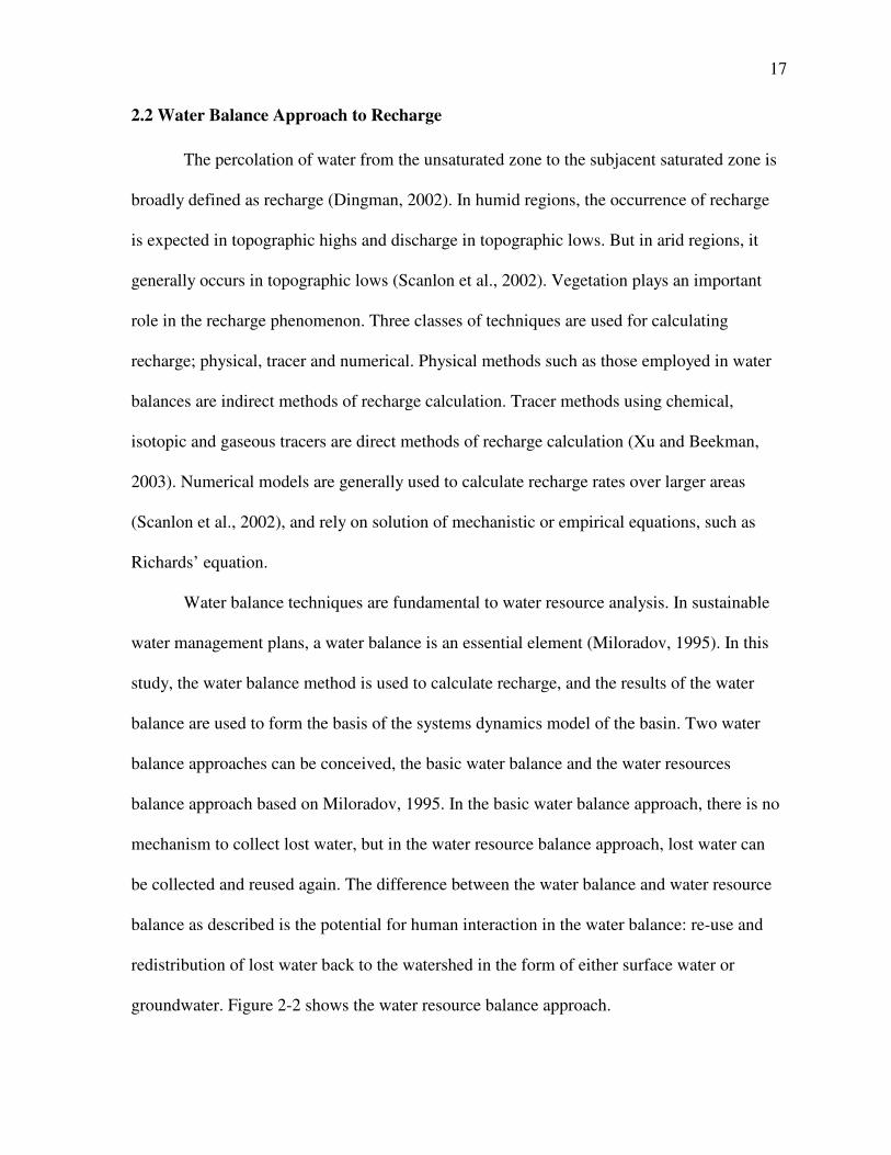
2.2 Water Balance Approach to Recharge

The percolation of water from the unsaturated zone to the subjacent saturated zone is

broadly defined as recharge (Dingman, 2002). In humid regions, the occurrence of recharge

is expected in topographic highs and discharge in topographic lows. But in arid regions, it

generally occurs in topographic lows (Scanlon et al., 2002). Vegetation plays an important

role in the recharge phenomenon. Three classes of techniques are used for calculating

recharge; physical, tracer and numerical. Physical methods such as those employed in water

balances are indirect methods of recharge calculation. Tracer methods using chemical,

isotopic and gaseous tracers are direct methods of recharge calculation (Xu and Beekman,

2003). Numerical models are generally used to calculate recharge rates over larger areas

(Scanlon et al., 2002), and rely on solution of mechanistic or empirical equations, such as

Richards’ equation.

Water balance techniques are fundamental to water resource analysis. In sustainable

water management plans, a water balance is an essential element (Miloradov, 1995). In this

study, the water balance method is used to calculate recharge, and the results of the water

balance are used to form the basis of the systems dynamics model of the basin. Two water

balance approaches can be conceived, the basic water balance and the water resources

balance approach based on Miloradov, 1995. In the basic water balance approach, there is no

mechanism to collect lost water, but in the water resource balance approach, lost water can

be collected and reused again. The difference between the water balance and water resource

balance as described is the potential for human interaction in the water balance: re-use and

redistribution of lost water back to the watershed in the form of either surface water or

groundwater. Figure 2-2 shows the water resource balance approach.

18

Figure 2-2: Water Resources Balance (Miloradov, 1995)

Water balance methods are based on the principle of conservation of mass. For an

arbitrary control volume over a given period of time, the difference between total input and

output will be balanced by the change of water storage with the volume (Equation 2-3).

StorageinChangeOutflowInflow =− (2-3)

Equation 2-4, after Sokolov and Chapman, (1974), shows the major inflows and outflows

components of water balance approach.

0=−∆−−−−++ ηSQQETQQP UOSOUISI (2-4)

The term P represents precipitation, QSI and QUI represent the surface and sub-surface

water inflow within water body from outside, QSO and QUO represent the surface and sub

surface water outflow from water body, ET is the evapotranspiration within the water body,

∆S is change in storage and η is the discrepancy (error) term. To simplify the analysis

presented here, the subsurface inflow and outflows is assumed to be zero for all scenarios

considered in this research. Equation 2-5 shows a general form of water balance approach

used in this study.

RQETP s =−− (2-5)

where, Qs is the discharge of river (surface water inflow) and R is the recharge.

Water available for use

Precipitation

Runoff

Surface Waters

Groundwaters

Additional water available for use

Lost water

19

The water balance approach is an indirect method of calculating recharge. In the

absence of direct measurements, the estimation of recharge by water balance models is the

best available tool (Faust et al., 2006). The major limitation of the water balance approach is

the dependence of one component to other (i.e., accuracy of recharge depends on the

accuracy of other components of water balance; Scanlon et al., 2002). Because of this

limitation, the usefulness of water balance methods in arid and semi-arid regions is

questioned by many researchers (Scanlon et al., 2002), primarily because of the uncertainty

in the estimation of evapotranspiration. In water balance approach, evapotranspiration is

typically more difficult to accurately quantify than precipitation and stream-flow and is large

in comparison to the magnitude of recharge.

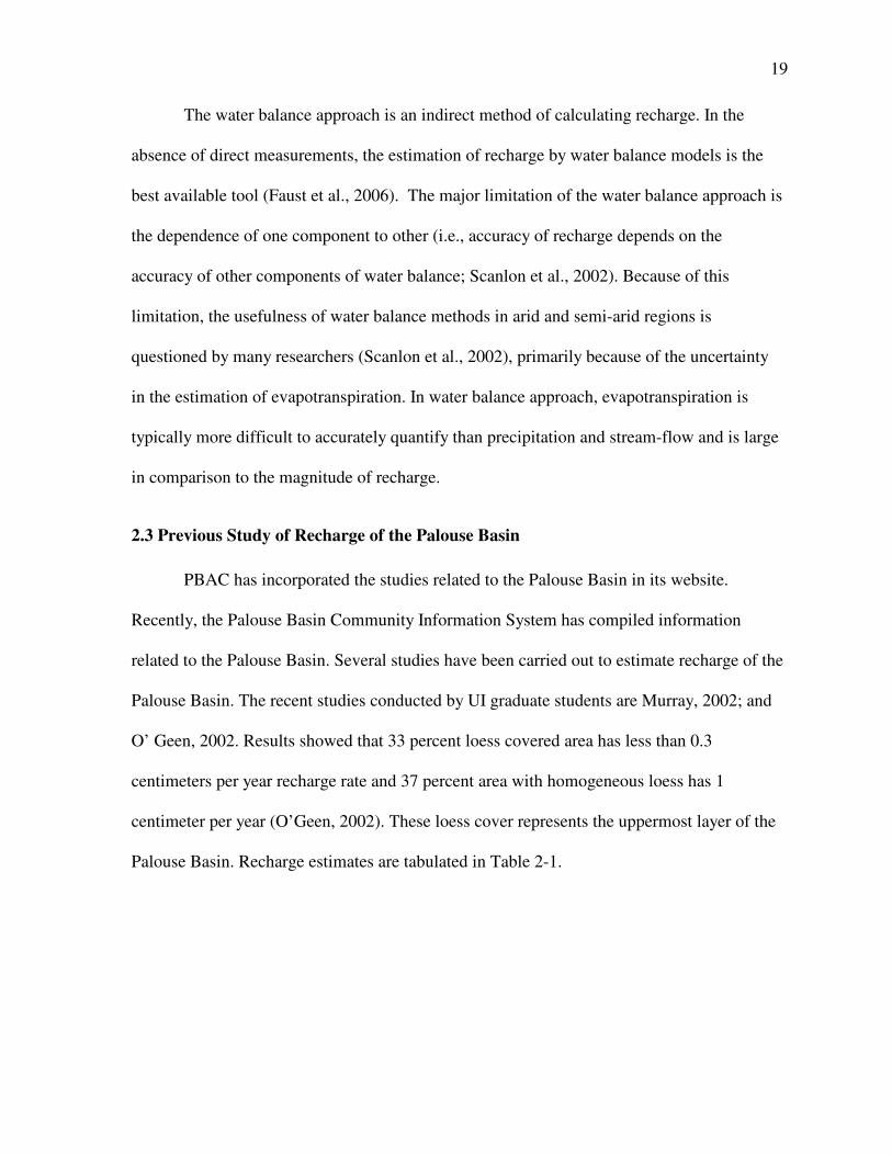
2.3 Previous Study of Recharge of the Palouse Basin

PBAC has incorporated the studies related to the Palouse Basin in its website.

Recently, the Palouse Basin Community Information System has compiled information

related to the Palouse Basin. Several studies have been carried out to estimate recharge of the

Palouse Basin. The recent studies conducted by UI graduate students are Murray, 2002; and

O’ Geen, 2002. Results showed that 33 percent loess covered area has less than 0.3

centimeters per year recharge rate and 37 percent area with homogeneous loess has 1

centimeter per year (O’Geen, 2002). These loess cover represents the uppermost layer of the

Palouse Basin. Recharge estimates are tabulated in Table 2-1.

20

Table 2-1: Estimated Recharge Rates (WRIA-34)

Recharge Rate Name

(cm yr-1

)

Palouse Loess

Stevens, 1960 3.0

Johnson, 1991 10.5

Muniz, 1991 2.5 to 10.3

O’ Brien and Others, 1997 (Pullman) 0.2 to 2

O’Geen, 2002 0.3-1

Wanapum

Foxworthy and Washburn, 19631 1.6

Barker, 1979 19.7

Smoot, 1987 9.15

Fealko and Fiedler, 2006 (Median) 8.5

Grande Ronde

Foxworthy and Washburn, 1963 1.6

Crosby and Chatters, 1965 Negligible

Barker, 1979 1.70

Smoot, 1987 4.83

Lum and others, 1990 5.08

Larson, 2000 Negligible

Not motioned (Wanapum or Grande

Ronde)

Bauer and Vaccaro, 1989 7.11 (Current)

Bauer and Vaccaro, 1989 10.42 (Pre-development)

Lum and others, 1990 7.11 (Total)

Baines, 1992 4.5

Bauer and Vaccaro, 1990 3.8

The recharge estimation of the Wanapum aquifer by Fealko, 2003 in the Pullman-

Moscow area is about 8.5 centimeters per year. Fealko used water balance approach applied

to the Paradise Creek Watershed to calculate these recharges. The isotope dating of the

groundwater of the Grande Ronde aquifer conducted by Kent Keller and others indicates the

21

age of the water as 10,000 years old (O'Brien et. al., 1996; Larson et. al., 2000).

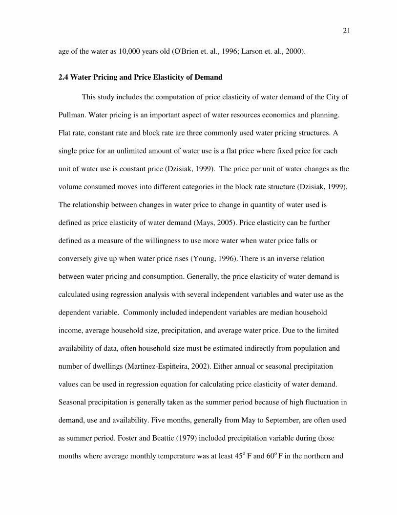
2.4 Water Pricing and Price Elasticity of Demand

This study includes the computation of price elasticity of water demand of the City of

Pullman. Water pricing is an important aspect of water resources economics and planning.

Flat rate, constant rate and block rate are three commonly used water pricing structures. A

single price for an unlimited amount of water use is a flat price where fixed price for each

unit of water use is constant price (Dzisiak, 1999). The price per unit of water changes as the

volume consumed moves into different categories in the block rate structure (Dzisiak, 1999).

The relationship between changes in water price to change in quantity of water used is

defined as price elasticity of water demand (Mays, 2005). Price elasticity can be further

defined as a measure of the willingness to use more water when water price falls or

conversely give up when water price rises (Young, 1996). There is an inverse relation

between water pricing and consumption. Generally, the price elasticity of water demand is

calculated using regression analysis with several independent variables and water use as the

dependent variable. Commonly included independent variables are median household

income, average household size, precipitation, and average water price. Due to the limited

availability of data, often household size must be estimated indirectly from population and

number of dwellings (Martinez-Espiñeira, 2002). Either annual or seasonal precipitation

values can be used in regression equation for calculating price elasticity of water demand.

Seasonal precipitation is generally taken as the summer period because of high fluctuation in

demand, use and availability. Five months, generally from May to September, are often used

as summer period. Foster and Beattie (1979) included precipitation variable during those

months where average monthly temperature was at least 45o F and 60o F in the northern and

22

southern regions of the United States respectively. Water demand is directly proportional to

temperature and inversely related to precipitation (Cook et al., 2001). In the summer, more

water is needed for irrigation if there is inadequate precipitation to maintain vegetation. If

precipitation is abundant, then the coefficient of precipitation is anticipated to be negative.

Study conducted by Linaweaver et al. (1967) use evapotraspiration in place of precipitation.

Available moisture or moisture defined by difference between the precipitation and

evapotranspiration can be used as alternative variables for precipitation. The common

exponential form of regression equation for calculating price elasticity of water demand is

shown in Equation 2-6.

43210 **** XXXX

r

X HPIPeQ = (2-6)

After taking log to the both sides, Equation 2-6 can be written as Equation 2-7. It is a

log linear empirical equation (Equation 2-7) used to model price elasticity of demand.

)ln(*)ln(*)ln(*)ln(*)ln( 43210 HXPXIXPXXQ r ++++= (2-7)

where, Q is the quantity of water consumption, Pr is water price, I is the median household

income ($ per year), P is the commutative precipitation (inch per year), H is the average

household size (number of people per household). X0 to X4 are the unknown least square

coefficients that should be estimated. IWR-MAIN, Water Demand Management Suite, has

used the following equation to calculate the predicted water use (Equation 2-8).

7654)3)((21 dddddFCdd RTHDHeMPaIQ = (2-8)

where, Q is the predicted water use in gallons per day, I is median household income

($1000’s), MP is effective marginal price ($ / 1000 gal), e is base of the natural logarithm,

FC is fixed charge ($), H is mean household size (person per household), T is maximum- day

temperature (degrees Fahrenheit), R is total seasonal rainfall (inches), a is intercept in

23

gallons/day and d1 to d7 are elasticity values for each independent or explanatory variable.

For a continuous demand function, price elasticity of water demand (ε) is calculated

by comparing the change in the quantity demanded (dQ) to the change in price (dPr)

(Equation 2-9).

)(*r

r

dP

dQ

Q

P=ε (2-9)

where, ε is the price elasticity of demand, Pr is the average water price, Q is the quantity of

water demand, dQ is the change in demand and dPr is the change in price.

2.4.1 Price elasticity in the Palouse Basin and nearby Cities

Lyman (1992) used a dynamic model to study water demand of City of Moscow.

Using number of climatic variables, price and income determinants and household

characteristics with survey data, peak and off-peaks effects were analyzed in water demand.

The price elasticity of seasonal demand for residential water is -0.65 for winter (off-peak)

and -3.33 for summer (peak) in Moscow, ID (Lyman, 1992).

Both short term and long term elasticity of marginal price is -0.3 in the Lewiston

Orchards Irrigation District (Rode, 2000). But the results for the marginal price, fixed price

and income variables are not statistically significant in entire City of Lewiston (Rode, 2000).

An effort to study dynamic aggregate water demand model for the Palouse Region (City of

Moscow and Pullman) by Peterson S.S., 1992 was inconclusive due to the insignificant

marginal variable (Rode, 2000).

2.5 System Dynamics Approach

In the 1950s, the System Dynamics Approach was initiated by J. W. Forrester at

Massachusetts Institute of Technology. Nonlinear dynamics form the general basis of

24

System Dynamics Approach (Ahmad and Simonovic, 2004). This approach can also be used

for shared vision planning. Shared vision planning involves discussion and debates as part of

the comprehensive decision making process (Stephenson, 2002). The emphasis of the shared

vision model is participation of stakeholders and technical experts together in a collaborative

planning process. Interactions between stakeholders and experts make complex feedback

mechanisms, similar to the natural feedback mechanisms in nature, and those between the

natural world and humans. For example, as water supplies diminish, the price of water tends

to increase, which reduces demand on the natural system.

Because of these numerous components and complex feedback mechanisms, it is

difficult to perform a sensitivity analysis using focused physical models. Sensitivity of

complex systems can be more readily explored using the systems approach. Xu et al. (2002)

emphasizes that difficulties mainly arise from the integration of social perspectives with the

technical elements. Results from more detailed and focused physical models can and should

inform system model development.

A basic challenge associated with any kind of modeling is to encapsulate the essential

aspects of real world phenomenon in the model. System modeling approach can be simple

enough for beginners who do not have the expertise required in other modeling efforts. The

approach facilitates understanding of the behavior of complex systems over time from causal

loop diagrams and stock and flows. Widely available systems software has user friendly

interfaces in which it is easy to develop and explain models. These types of models are

excellent for cause and effect analysis (sensitivity analysis) simulation. Because of these

factors, the System Dynamics Approach can be used as a useful tool in shared vision

planning, and facilitates interaction between experts with different disciplinary backgrounds.

25

Commercially available system dynamics software includes AnyLogic, Powersim,

Studio, CONSIDEO, Vensim, STELLA and iThink, MapSys, and Simile. STELLA Version

9 was used for developing the models in this study because of its solid reputation and wide

use. There are four basic model components in the STELLA software: stocks, flows,

converters and connecters. Stocks are able to accumulate or deplete things (such as

groundwater reservoirs) over time. It is a state variable which helps to define the state of

system. Flows control the changes of magnitude of stocks, and can be viewed as inputs and

outputs to stocks. Converters have a wide range of functions such as holding external factors

affecting stocks and flows (e.g., growth rates), data, numerical constants, equations and

graphical relationships. Finally, connecters are used for transferring information between

model components. Information can be transferred among all components with connecters

except for stocks (the storage in which are completely controlled by flows). Ghost

components help to make replicas, aliases, or shortcuts for individual stocks, flows, and

converters. Model boundaries are represented in STELLA by clouds. Source cloud is infinite

source of inflow and sink cloud is infinite sink for outflow. Figure 2-3 shows the basic

components of STELLA.

Stock

Inflow Outflow

Converter

Source Cloud Sink Cloud

Connecter

Figure 2-3: Components of STELLA Software

26

Use of the System Dynamics Approach in water resources planning accelerated in the

1990s. Some of the important works in this approach in water resource planning were

drought studies (Keyes and Palmer, 1993), modeling sea-level rise in a coastal area (Matthias

and Frederick, 1994) and river basin planning (Palmer, 1998; Ahmad et al., 2004).

Simonovic et al., (1997) used the System Dynamics Approach for planning and policy

analysis for the Nile River Basin in Egypt. Simonovic and his colleagues further applied this

approach in flood prediction, control and damages calculation, hydropower generation and

climate changes sectors. System Dynamics approach is used for community based water

planning in the Middle Rio Grande in north-central New Mexico (Tidwell et al., 2003). Dr.

Richard Palmer, Professor of Civil and Environmental Engineering, University of

Washington has developed the “Fairweather” model in the STELLA software as an example

for his students. “Fairweather” model integrates several aspects of watershed management,

such as hydrology, population dynamics, demand forecast, river rafting, economic metrics,

water supply, and water laws.

27

CHAPTER III

DATA REQUIRED FOR MODELING

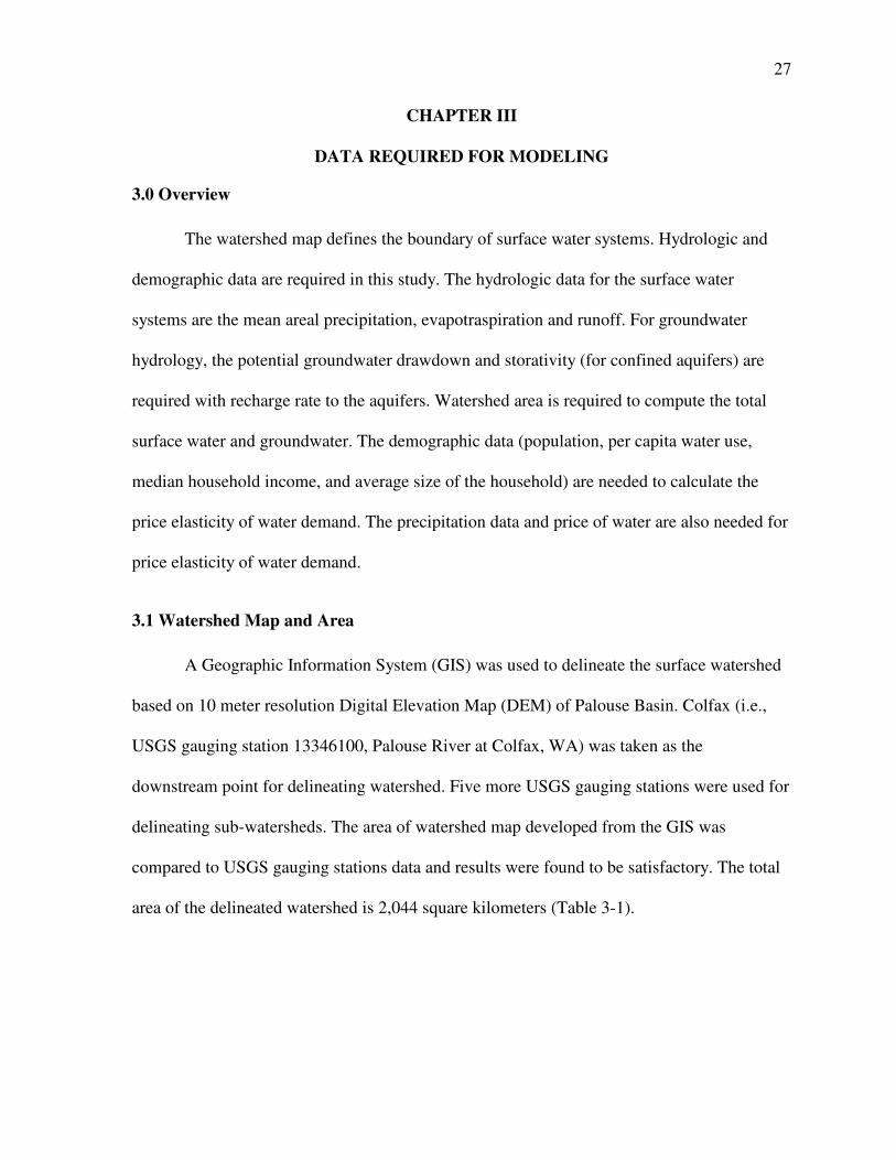
3.0 Overview

The watershed map defines the boundary of surface water systems. Hydrologic and

demographic data are required in this study. The hydrologic data for the surface water

systems are the mean areal precipitation, evapotraspiration and runoff. For groundwater

hydrology, the potential groundwater drawdown and storativity (for confined aquifers) are

required with recharge rate to the aquifers. Watershed area is required to compute the total

surface water and groundwater. The demographic data (population, per capita water use,

median household income, and average size of the household) are needed to calculate the

price elasticity of water demand. The precipitation data and price of water are also needed for

price elasticity of water demand.

3.1 Watershed Map and Area

A Geographic Information System (GIS) was used to delineate the surface watershed

based on 10 meter resolution Digital Elevation Map (DEM) of Palouse Basin. Colfax (i.e.,

USGS gauging station 13346100, Palouse River at Colfax, WA) was taken as the

downstream point for delineating watershed. Five more USGS gauging stations were used for

delineating sub-watersheds. The area of watershed map developed from the GIS was

compared to USGS gauging stations data and results were found to be satisfactory. The total

area of the delineated watershed is 2,044 square kilometers (Table 3-1).

28

Table 3-1: Area of Sub-Watersheds

Area of Sub-Watersheds (Local

Area ) USGS Gauging

Stations Site Name

(km2)

13349210 Palouse River below South Fork at Colfax

(Entire Basin) 2,044

13345000 Palouse River near Potlatch, ID 816.36

13345300 Palouse River at Palouse, WA 69.77

13346100 Palouse River at Colfax, WA (North Fork) 388.45

N/A1 South Fork above Colfax, WA (local) 439.03

13346800 Paradise Creek at UI at Moscow, ID 45.65

13348000 South Fork Palouse River at Pullman, WA 284.35

Total 2,044 1. No USGS gage exists on the South Fork of the Palouse upstream of Colfax. The stream flows were

computed as the difference between USGS gauge 13346100, downstream of the confluence of the South Fork and the main stem of the Palouse River and USGS gage 13348000 located on the main stem of the Palouse River just upstream of the confluence near Colfax.

3.2 Geology of Palouse Basin Aquifer

The geology of an aquifer helps to understand the spatial extent and characteristics of

the aquifer material matrix, its hydrological and geological separation and volume.

Numerous research activities have been carried out to understand the geology of the Palouse

Basin within the last thirty years. John Bush and his colleagues from University of Idaho and

Washington State University have led these efforts. The geology of the Palouse Basin is

highly complex and therefore it is difficult to understand the groundwater basin. According

to John Bush and his colleagues, the Palouse Basin aquifer can be divided into six regions

determined in part by geologic variations, and in part by information availability. They are

Moscow, Pullman, Colfax, Viola, Palouse and Uniontown (Figure 1-3). It is important to

note that the division of the basin into these regions does not imply hydrologic connections

or lack thereof.

The Palouse Basin lies within the Columbia River Basalt Group (CRBG). The uppermost

29

layer of the Palouse loess ranges from 0 to 76 meters (PBAC, 1990). Groundwater in the

Palouse loess is in unconfined state (Foxworthy and Washburn, 1963). As previously

discussed, there are upper and lower aquifers in the basin. The existence of the upper

Wanapum aquifer seems significant in all groundwater basins with comparatively thin layer

in Pullman area (46 meters) (Bush and Hinds, 2006). The Moscow Wanapum is productive

for groundwater extraction whereas the Pullman Wanapum is unproductive (Leek, 2006).

The hydrologic and geologic characteristics of the Grande Ronde also vary within the

different groundwater basins. The Grande Ronde of Pullman and Moscow region appears as

a confined aquifer (Fealko, 2003, Holom, 2006). But Bandon and Osiensky, 2007 mentioned

that the vicinity of Moscow Well 2 (located in the Wanapum aquifer) is not confined. The

Uniontown groundwater region is outside the designated surface water watershed area and

not accounted to any computation in this study. Table 3-2 shows the estimated volume, areas

and thickness of groundwater regions. It should be noted that the confidence in these

estimates varies greatly depending on available information with the best estimates being

near population centers. Figure 3-1 shows the schematic of the geology of the aquifers and

the locations of wells.

30

Table 3-2: Aquifer Volume, Area and Thickness (Bush and Hinds, 2006)

Average Wanapum Thickness

Average Grande Ronde

Thickness

Wanapum Volume

Grande Ronde Volume

Wanapum Area

Grande Ronde Area

Name of Groundwater

Regions

(m) (m) (m3) (m3) (km2) (km2)

Moscow 137 259 1.12E+10

Sediments-60% Basalt-40%

1.66E+10 Sediments-

65% Basalt-35%

81.75 63.94

Pullman Upper Grande Ronde (productive)

46 305 1.15E+10


7.20E+10 Sediments-

10% Basalt-90%

252.08 235.97

Pullman Lower Grande Ronde

+ Imnaha1 305

3.60E+10 Lower Grande

Ronde + Imnaha

Sediments- 10%

Basalt-90%

Viola 137 244 3854050289


5185964728 Sediments-

65% Basalt-35%

28.08 21.25

Palouse 85 152 1.62E+10


1.13E+10 Sediments -

60% Basalt-40%

190.12 74.32

Colfax 122 244 4.22E+10


8.10E+10 Sediments-5%

Basalt-95% 346.06 332.13

Uniontown 122 457-549 9.44E+10


3.17E+11 to 4.19E+11

(no wells, only outcrops along

snake river)

782.71

763.86

Uniontown Saddle

mountain

46 3.57E+10


1. Imnaha is lowermost layer of the Columbia Basin Basalt Group.

31

Figure 3-1: Schematic East West Cross Section of Study Area (Owsley, 2003)

32

3.3 Aquifer Volume

Porosity is the volume of water storage per volume of aquifer in an unconfined

aquifer. Likewise, the storage coefficient or storativity is volume of water storage per volume

of aquifer in a confined aquifer (White and Revees, 2002). Both the Wanapum and Grande

Ronde aquifers are confined; the storativity is thus used for calculating volume of water in

the aquifers. By definition, storativity is the volume of water that an aquifer releases per unit

surface area under a unit decline of hydraulic head. Alternatively, storativity is the ratio of

volume of water in confined aquifer to volume of aquifer (Equation 3-1).

AquiferofVolume

AquiferConfinedinWaterofVolumeSyStorativit =)( (3-1)

White (2002) computed volume of groundwater in New Zealand by using average saturated

thickness (Equation 3-2).

cofficientstorageaverageaquiferofareathicknesssaturatedAverageVolume **= (3-2)

Storativity of the Palouse Basin Grande Ronde ranges between 10-3 and 10-5 based on

aquifer discharge tests (Osiensky, 2006). A base value of 10-3 was used in the model, with an

allowed range from 10-2 to 10-5. The lowering of the groundwater level near the pumping

well is defined as drawdown (Mullen, 2007). The average potential groundwater drawdown

in the current infrastructure was calculated as a difference between the approximate pumping

water level and the pump intake elevation in the wells (Figure 3-2). There is also wide

variation in the thickness of the Wanapum and Grande Ronde regions. So, geometrical

methods (i.e., average potential drawdown depth, surface area) are used for calculating

groundwater volume in these aquifers. The average maximum potential groundwater

drawdown is computed at the bottom of the well. Potential maximum groundwater

drawdown data were obtained from the four entities (Table 3-3).

33

Well

Static water level,

Pumping level

Bottom of pump

Bottom of well

Figure 3-2: Definition Sketch for Calculating Volume of Water in the Aquifers

Equation 3-3 was used to calculate volume of water in aquifers in the Palouse Basin.

HASV ∆= ** (3-3)

where, V is the volume of water in aquifer, S is the storativity, ∆H is the water level change

used in computing the volume and A is the surface area of aquifer. The total groundwater

volume of the aquifer is calculated from the average saturated depth. ∆H, the potential

drawdown, is used calculate the volume of the groundwater which is smaller than the total

saturated thickness of the aquifer. The potential groundwater drawdown of Colfax, Palouse

and Viola are assumed to be similar to the Pullman groundwater region.

current drawdown

potential drawdown

maximum

potential drawdown

saturated

thickness

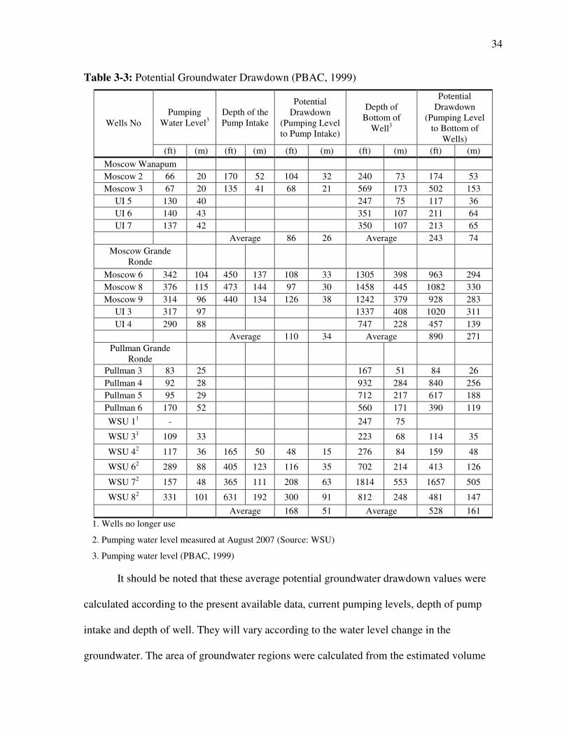
34

Table 3-3: Potential Groundwater Drawdown (PBAC, 1999)

Pumping Water Level3

Depth of the Pump Intake

Potential Drawdown

(Pumping Level to Pump Intake)

Depth of Bottom of

Well3

Potential Drawdown

(Pumping Level to Bottom of

Wells)

Wells No

(ft) (m) (ft) (m) (ft) (m) (ft) (m) (ft) (m)

Moscow Wanapum

Moscow 2 66 20 170 52 104 32 240 73 174 53

Moscow 3 67 20 135 41 68 21 569 173 502 153

UI 5 130 40 247 75 117 36

UI 6 140 43 351 107 211 64

UI 7 137 42 350 107 213 65

Average 86 26 Average 243 74

Moscow Grande Ronde

Moscow 6 342 104 450 137 108 33 1305 398 963 294

Moscow 8 376 115 473 144 97 30 1458 445 1082 330

Moscow 9 314 96 440 134 126 38 1242 379 928 283

UI 3 317 97 1337 408 1020 311

UI 4 290 88 747 228 457 139


Pullman Grande Ronde

Pullman 3 83 25 167 51 84 26

Pullman 4 92 28 932 284 840 256

Pullman 5 95 29 712 217 617 188

Pullman 6 170 52 560 171 390 119

WSU 11 - 247 75

WSU 31 109 33 223 68 114 35

WSU 42 117 36 165 50 48 15 276 84 159 48

WSU 62 289 88 405 123 116 35 702 214 413 126

WSU 72 157 48 365 111 208 63 1814 553 1657 505

WSU 82 331 101 631 192 300 91 812 248 481 147


1. Wells no longer use

2. Pumping water level measured at August 2007 (Source: WSU)

3. Pumping water level (PBAC, 1999)

It should be noted that these average potential groundwater drawdown values were

calculated according to the present available data, current pumping levels, depth of pump

intake and depth of well. They will vary according to the water level change in the

groundwater. The area of groundwater regions were calculated from the estimated volume

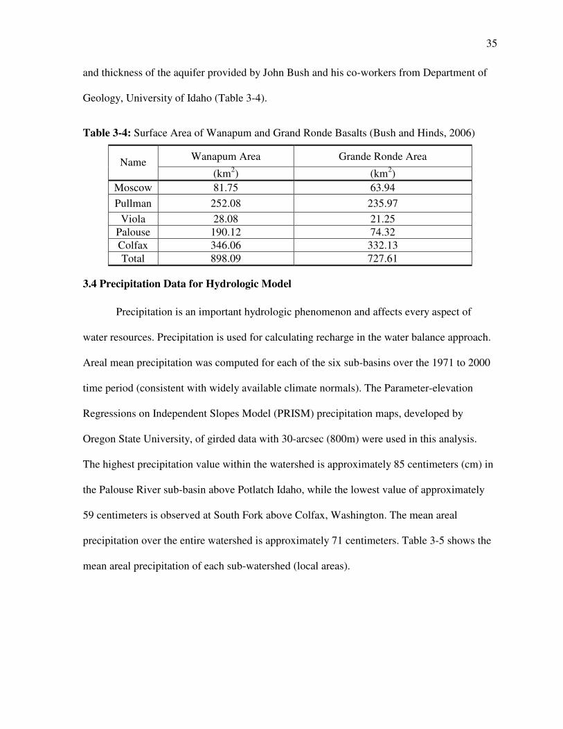
35

and thickness of the aquifer provided by John Bush and his co-workers from Department of

Geology, University of Idaho (Table 3-4).

Table 3-4: Surface Area of Wanapum and Grand Ronde Basalts (Bush and Hinds, 2006)

Wanapum Area Grande Ronde Area Name

(km2) (km2)

Moscow 81.75 63.94

Pullman 252.08 235.97

Viola 28.08 21.25

Palouse 190.12 74.32

Colfax 346.06 332.13

Total 898.09 727.61

3.4 Precipitation Data for Hydrologic Model

Precipitation is an important hydrologic phenomenon and affects every aspect of

water resources. Precipitation is used for calculating recharge in the water balance approach.

Areal mean precipitation was computed for each of the six sub-basins over the 1971 to 2000

time period (consistent with widely available climate normals). The Parameter-elevation

Regressions on Independent Slopes Model (PRISM) precipitation maps, developed by

Oregon State University, of girded data with 30-arcsec (800m) were used in this analysis.

The highest precipitation value within the watershed is approximately 85 centimeters (cm) in

the Palouse River sub-basin above Potlatch Idaho, while the lowest value of approximately

59 centimeters is observed at South Fork above Colfax, Washington. The mean areal

precipitation over the entire watershed is approximately 71 centimeters. Table 3-5 shows the

mean areal precipitation of each sub-watershed (local areas).

36

Table 3-5: Mean Areal Precipitation of Palouse Basin Sub-Watersheds

Precipitation

USGS Gauging Stations

Site Name

(cm)

13349210 Entire Basin 70.9

13346100 Palouse river at Colfax, WA (North Fork) 59.3

N/A South Fork above Colfax, WA (local) 58.9


13345300 Palouse river at Palouse, WA 66.7

13346800 Paradise Creek at University of Idaho at Moscow,

ID 75.1


3.5 Surface Runoff

Surface runoff is used in the water balance approach. Daily discharge data (1971-

2000) from USGS gauging stations were used to calculate surface runoff. Table 3-6 shows

USGS gauging stations with missing daily discharge data and the USGS gauging stations

used to fill the missing daily discharges. Missing data were estimated with linear regression

among the USGS gauging stations.

Table 3-6: Period of Availability of Daily Discharge of USGS Gauging Stations

Stations (Y)

Site Name Stations used for filling gap

(X)

Linear Regression Equation

Period of Availability

13349210 Entire Basin 13345000 y = 1.3951x + 22.83,

R2 = 0.8916 1963/10/01-1995/09/30

13345300 Palouse River at Palouse,

WA 13345000

y = 1.0381x + 1.54, R2 = 0.9708

04/19/1973-10/02/1980

13346100 Palouse River at Colfax,

WA (North Fork) 13345000

y = 1.0798x + 13.60, R2 = 0.9352

10/1/1963-05/31/1979

13346800 Paradise Creek at UI at

Moscow, ID 13348000

y = 0.2032x - 0.29, R2 = 0.719

10/01/1978-09/30/2006

13348000 South Fork Palouse river

at Pullman, WA 13346800

y = 3.5385x + 10.11, R2 = 0.719

02/01/1934-09/30/2006

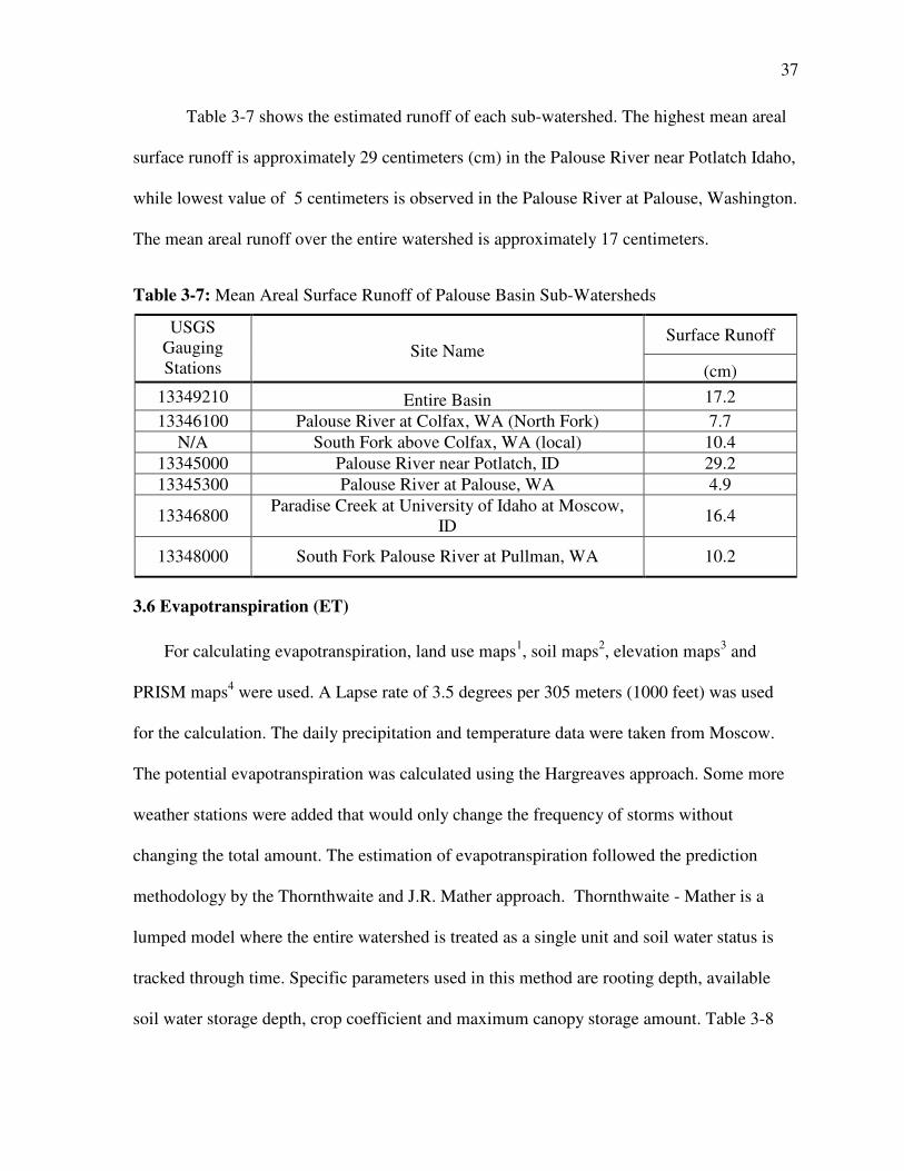
37

Table 3-7 shows the estimated runoff of each sub-watershed. The highest mean areal

surface runoff is approximately 29 centimeters (cm) in the Palouse River near Potlatch Idaho,

while lowest value of 5 centimeters is observed in the Palouse River at Palouse, Washington.

The mean areal runoff over the entire watershed is approximately 17 centimeters.

Table 3-7: Mean Areal Surface Runoff of Palouse Basin Sub-Watersheds

Surface Runoff USGS Gauging Stations

Site Name (cm)






13346800 Paradise Creek at University of Idaho at Moscow,

ID 16.4


3.6 Evapotranspiration (ET)

For calculating evapotranspiration, land use maps1, soil maps2, elevation maps3 and

PRISM maps4 were used. A Lapse rate of 3.5 degrees per 305 meters (1000 feet) was used

for the calculation. The daily precipitation and temperature data were taken from Moscow.

The potential evapotranspiration was calculated using the Hargreaves approach. Some more

weather stations were added that would only change the frequency of storms without

changing the total amount. The estimation of evapotranspiration followed the prediction

methodology by the Thornthwaite and J.R. Mather approach. Thornthwaite - Mather is a

lumped model where the entire watershed is treated as a single unit and soil water status is

tracked through time. Specific parameters used in this method are rooting depth, available

soil water storage depth, crop coefficient and maximum canopy storage amount. Table 3-8

38

shows the estimated evapotraspiration of each sub-watershed.

1. Land use Map reference: University of Idaho (UI) Library, U.S. Geological Survey, 20000329, Multi-

resolution Land Characterization for Idaho: University of Idaho library, Moscow, Idaho (30m resolution).

2. Soils Map: Soil Survey Geographic (SSURGO) Database, U.S. Department of Agriculture, Natural

Resources Conservation Service, 20060109 Fort Worth, Texas (30 m resolution),

URL:<http://www.ftw.nrcs.usda.gov/ssur_data.html>

3. Elevation Map: U.S. Geological Survey (USGS), EROS Data Center 1999, National Elevation, Dataset,

raster digital data Sioux Falls, SD (30 m resolution), http://gisdata.usgs.net/ned/>

4. PRISM maps (1971-2000) 800 m resolution,

http://www.ocs.oregonstate.edu/prism/products/viewer.phtml?file=/pub/prism/us_30s/grids/tmax/Normals/us_t

max_1971_2000.14.gz&year=1971_2000&vartype=tmax&month=14&status=final

Table 3-8: Mean Areal Evapotranspiration of Palouse Basin Sub-Watersheds

Evapotranspiration USGS Gauging Stations

Site Name (cm)






13346800 Paradise Creek at University of Idaho at Moscow, ID 49.8


The highest mean areal evapotraspiration is approximately 54 centimeters (cm) in the

Palouse River near Potlatch ID, while lowest value of approximately 45 centimeters is

observed in the South Fork above Colfax, Washington (North Fork). The mean areal

evapotraspiration over the entire watershed is approximately 49 centimeters.

3.7 Recharge to Wanapum

The recharge rate to the Wanapum aquifer is of primary importance. At present, even

though the major portion of water is extracted from the Grande Ronde, the recharge to

39

Wanapum represents the total amount of water that reaches to the groundwater basins. The

recharge rate to the Wanapum aquifer was calculated following Equation 2-5, using the basic

water balance approach over the 1971 to 2000 time period. Table 3-9 shows the recharge to

the entire Palouse watershed and the corresponding sub-watersheds.

Table 3-9: Mean Areal Recharge of Palouse Basin Sub-Watersheds

Precipitation ET

(Brooks, 2006)

Runoff (Fiedler, 2006)

Recharge Site Name

USGS Gauging Stations

(cm) (cm) (cm) (cm)

Entire Basin 13349210 70.9 49.0 17.2 4.7

Palouse River at Colfax, WA (North Fork)

13346100 59.3 45.2 7.7 6.4

South Fork above Colfax, WA (local)

N/A 58.9 44.8 10.4 3.7

Palouse River near Potlatch, ID

13345000 84.7 53.8 29.2 1.7

Palouse River at Palouse, WA

13345300 66.7 46.6 4.9 15.2

Paradise Creek at University of Idaho at

Moscow, ID 13346800 75.1 49.8 16.4 8.9

South Fork Palouse River at Pullman, WA

13348000 66.1 46.7 10.2 9.2

The average recharge rate to the entire watershed is 4.7 centimeters per year, varying

from 1.9 to 15.2 centimeters per year. The recharge computed in this study (Table 3-9) is

within the range of previous studies. The lowest value of recharge by Foxworthly and

Washburn (1963) is 1.6 centimeters and 19.7 centimeters per year as highest value by Baker

(1963).

3.8 Recharge to Grande Ronde

The Grande Ronde is commonly thought to receive little recharge. This assumption

is supported by aquifer water age dating (Crosby and Chatters, 1965 and Larson et al., 2000).

However, other researchers (Table 2.1) argued and calculated the existence of recharge from

Wanapum to Grande Ronde. The recharge rate to the Grande Ronde is assumed to be

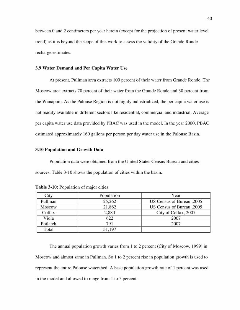
40

between 0 and 2 centimeters per year herein (except for the projection of present water level

trend) as it is beyond the scope of this work to assess the validity of the Grande Ronde

recharge estimates.

3.9 Water Demand and Per Capita Water Use

At present, Pullman area extracts 100 percent of their water from Grande Ronde. The

Moscow area extracts 70 percent of their water from the Grande Ronde and 30 percent from

the Wanapum. As the Palouse Region is not highly industrialized, the per capita water use is

not readily available in different sectors like residential, commercial and industrial. Average

per capita water use data provided by PBAC was used in the model. In the year 2000, PBAC

estimated approximately 160 gallons per person per day water use in the Palouse Basin.

3.10 Population and Growth Data

Population data were obtained from the United States Census Bureau and cities

sources. Table 3-10 shows the population of cities within the basin.

Table 3-10: Population of major cities

The annual population growth varies from 1 to 2 percent (City of Moscow, 1999) in

Moscow and almost same in Pullman. So 1 to 2 percent rise in population growth is used to

represent the entire Palouse watershed. A base population growth rate of 1 percent was used

in the model and allowed to range from 1 to 5 percent.

City Population Year

Pullman 25,262 US Census of Bureau ,2005

Moscow 21,862 US Census of Bureau ,2005

Colfax 2,880 City of Colfax, 2007

Viola 622 2007

Potlatch 791 2007

Total 51,197

41

3.11 Economic Data

The residential price elasticity of water demand of the City of Pullman was

calculated. Because of the limited availability of these data across the basin, the city of

Pullman was taken as representative of the basin, and used to develop a single price elasticity

relationship. The City of Pullman is the largest population center in Palouse Basin. Single

family, total residential families and total population are three economic scenarios for

calculating price elasticity of water demand. Total residential households includes single,

duplex, multiple, group and mobile homes. These water consumption estimates did not

include the industrial, commercial and schools and offices.

The independent variables for price-elasticity of water demand includes precipitation,

annual household income, average household size, marginal water price, and fixed water

price; whereas the monthly water use is dependent variable. Median household income in

dollars, marginal and fixed price in dollars, precipitation data in inches and household size

are the independent variables. In the Economic Scenario 1, the dependent variable is monthly

water use by single family per household per 100 cubic feet whereas in Economic Scenario 2,

monthly water use per household per 100 cubic feet by total residential sector. Finally, in

Economic Scenario 3 the dependent variable is mean monthly household water use by the

total population. Equation 3-4 shows the water use per household per 100 cubic feet of single

family class.

100*

)(100

33

HouseholdsFamilySingleofNumber

ftFamilySinglebyUseWaterftperhouseholdperUseWater = (3-4)

Table 3-11 shows the detailed price structures of City of Pullman from the year 1971

to 2006.

42

Table 3-11: Marginal and Fixed Price Rates of City of Pullman

Marginal Price Ready to

serve

($/100 ft3) Base Fee ($) Year

(501-1000) ft3 (1001-2000) ft3 (2001-3000) ft3 Over 3001 ft3

1971 0.32 0.24 0.16 0.12 2.75

(0-500) ft3 (500-2000) ft3 Above 2000 ft3

1972 0.44 0.36 0.20 2

Volume charge above 500 ft3 ($) 1 inch meter

size

1981 0.29 1.8

1981 0.34 5.2

1988 0.51 7.8

1991 0.55 8.46

1992 0.6 9.18

1993 0.65 9.96

1994 0.7 10.81

1995 0.71 10.98

1996 0.75 11.53

Volume charge above 500 ft3

Winter (October – May) Summer(June-

September)

1 inch meter size

1998 0.88 20.09

1999 0.92 1.13 20.99

2000 0.96 1.18 21.93

2000 0.96 1.18 21.93

2001 1 1.23 22.92

2002 1.05 1.29 23.95

2003

Winter Summer

(500-800) ft3 Over 800 ft3 (500-800) ft3 (801-2000) ft3 Over 2000ft3

($/100 ft3)

1 inch meter size

2004 1.1 1.15 1.3 1.4 1.75 24.9

2005 1.14 1.2 1.35 1.46 1.82 25.9

2006 1.19 1.24 1.41 1.51 1.89 26.93

Source City of Pullman

The marginal price of the City of Pullman is based on the volumetric water use. Up to

500 cubic feet for any kind of user class, no marginal price is to be paid but certain ready to

serve (fixed price) is to be paid whether water is used or not. The fixed charge also varies

according to the user class and size of the meter (Lamar and Weppner, 1995). The city of

Pullman has increasing block rate of marginal water price varying in the peak (summer) and

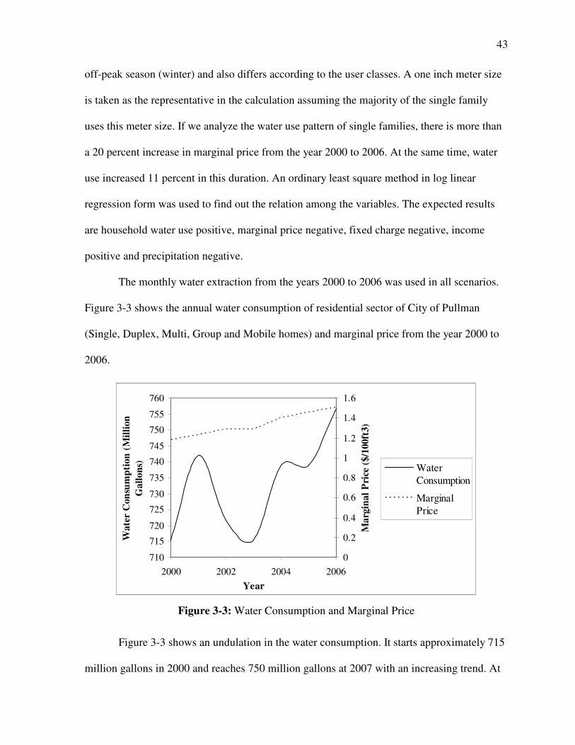
43

off-peak season (winter) and also differs according to the user classes. A one inch meter size

is taken as the representative in the calculation assuming the majority of the single family

uses this meter size. If we analyze the water use pattern of single families, there is more than

a 20 percent increase in marginal price from the year 2000 to 2006. At the same time, water

use increased 11 percent in this duration. An ordinary least square method in log linear

regression form was used to find out the relation among the variables. The expected results

are household water use positive, marginal price negative, fixed charge negative, income

positive and precipitation negative.

The monthly water extraction from the years 2000 to 2006 was used in all scenarios.

Figure 3-3 shows the annual water consumption of residential sector of City of Pullman

(Single, Duplex, Multi, Group and Mobile homes) and marginal price from the year 2000 to

2006.

710

715

720

725

730

735

740

745

750

755

760

2000 2002 2004 2006

Year

Wa

ter

Con

sum

pti

on

(M

illi

on

Ga

llo

ns)

0

0.2

0.4

0.6

0.8

1

1.2

1.4

1.6

Ma

rgin

al

Pri

ce (

$/1

00

ft3)

Water

Consumption

Marginal

Price

Figure 3-3: Water Consumption and Marginal Price

Figure 3-3 shows an undulation in the water consumption. It starts approximately 715

million gallons in 2000 and reaches 750 million gallons at 2007 with an increasing trend. At

44

the same time, the marginal price of water is increasing. Figure 3-4 shows the monthly water

consumption trend of residential sector from the year 2000 to 2006. In summer time, water

consumption is relatively higher than winter period.

0.000

20.000

40.000

60.000

80.000

100.000

120.000

2000 2001 2002 2003 2004 2005 2006 2007

Year

Mo

nth

ly W

ate

r C

on

sum

pti

on

(Mil

lio

n G

all

on

s)

Residential

Sector

Figure 3-4: Monthly Water Consumption of Residential Sector of City of Pullman

There are other specific limitations in this study. Because of a lack of exact service

connections, numbers of single family household data are used from some literature reviews.

The population, household size and median household income are generally calculated

annually and some are calculated on a decade basis. So, there is difficulty in collecting these

data in monthly basis. So these data are linearly interpolated in monthly basis. The household

level survey data is more precise and effective for calculating price elasticity. Table 3-12

shows the sample data for calculating price elasticity of water demand of single family.

Appendix B presents comprehensive data set of City of Pullman for economic analysis.

45

Table 3-12: Sample Data for Economic Analysis of Single Family, Pullman, Washington

Year Fixed Price Marginal

Price

Median Household

income Precipitation

(2000)

Household Water Use

/100 ft3 $ (1inch meter size) ($/100 ft3)

Household size

($ / year) (in / month)

Month Q FP MP H I P

January 6.11 21.93 0.96 2.24 21,662 1.90

February 5.67 21.93 0.96 2.24 21,696 2.66

March 6.57 21.93 0.96 2.24 21,731 2.31

April 5.81 21.93 0.96 2.24 21,765 1.21

May 7.67 21.93 0.96 2.24 21,799 2.14

June 10.92 21.93 1.18 2.24 21,833 1.19

July 16.47 21.93 1.18 2.24 21,867 0.01

August 23.14 21.93 1.18 2.24 21,902 0.04

September 17.78 21.93 1.18 2.24 21,936 1.51

October 8.15 21.93 0.96 2.24 21,970 1.65

November 7.18 21.93 0.96 2.24 22,004 1.86

December 6.05 21.93 0.96 2.24 22,038 1.44

Due to the limitation of this study, the monthly commutative time series data is used.

These types of aggregated time series data have lot of complications as if it is difficult to

understand the behavior of individual households.

46

CHAPTER IV

MODEL DEVELOPMENT SCENARIOS

4.0 Overview

A systems model of the Palouse Basin water resources was constructed using

STELLA software to evaluate water resources sustainability. The model is founded on the

data and water balance approach presented in Chapter 3, and includes a demand component

and basic economic considerations. Two versions were created: a lumped model that treats

the entire basin as a single unit designated the “Simple Model” (SM), and a “Hydrologically

Separated Model” (HSM) model that divides the basin into sub-units to account for some

spatial differences in supply and demand. Since many of the variables were uncertain,

selected parameters were allowed to vary, and uncertainty analysis was performed. This

chapter describes the conceptual modeling approach and its construction. Appendix C

presents the models as implemented in STELLA.

The Hydrological Model, Population and Demand Forecast Module, Surface Water

Utilization Module and Economic Module are described herein. The most common term

(groundwater aquifer) here indicates the stock which accumulates and depletes over time.

Basically, the Wanapum and Grande Ronde aquifers are stocks or reservoirs in the System

Dynamics Approach. The term “recharge” indicates flow which changes the magnitude of

reservoirs over time. The extraction of water from the groundwater aquifers and surface

water systems are flows.

4.1 Interactions among the Models

The forecasted population from the population model is used by demand forecast

model. Demand model uses per capita per day water use for forecasting water demand. After

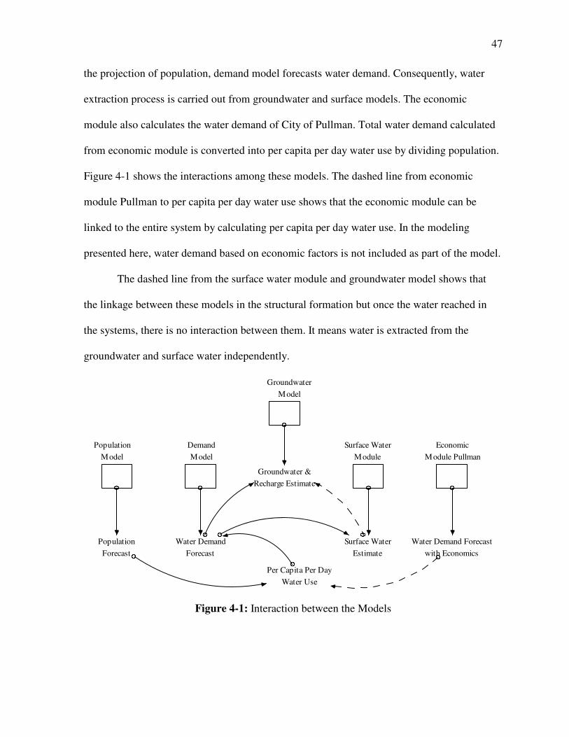
47

the projection of population, demand model forecasts water demand. Consequently, water

extraction process is carried out from groundwater and surface models. The economic

module also calculates the water demand of City of Pullman. Total water demand calculated

from economic module is converted into per capita per day water use by dividing population.

Figure 4-1 shows the interactions among these models. The dashed line from economic

module Pullman to per capita per day water use shows that the economic module can be

linked to the entire system by calculating per capita per day water use. In the modeling

presented here, water demand based on economic factors is not included as part of the model.

The dashed line from the surface water module and groundwater model shows that

the linkage between these models in the structural formation but once the water reached in

the systems, there is no interaction between them. It means water is extracted from the

groundwater and surface water independently.

Population

Model

Demand

Model

Groundwater

Model

Surface Water

Module

Economic

Module Pullman

Population

Forecast

Water Demand

Forecast

Groundwater &

Recharge Estimate

Surface Water

Estimate

Water Demand Forecast

with Economics

Per Capita Per Day

Water Use

Figure 4-1: Interaction between the Models

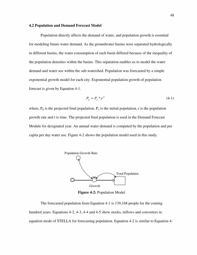
48

4.2 Population and Demand Forecast Model

Population directly affects the demand of water, and population growth is essential

for modeling future water demand. As the groundwater basins were separated hydrologically

in different basins, the water consumption of each basin differed because of the inequality of

the population densities within the basins. This separation enables us to model the water

demand and water use within the sub-watershed. Population was forecasted by a simple

exponential growth model for each city. Exponential population growth of population

forecast is given by Equation 4-1.

rt

op ePP *= (4-1)

where, Pp is the projected final population, Po is the initial population, r is the population

growth rate and t is time. The projected final population is used in the Demand Forecast

Module for designated year. An annual water demand is computed by the population and per

capita per day water use. Figure 4-2 shows the population model used in this study.

Total Population

Growth

Population Growth Rate

Figure 4-2: Population Model

The forecasted population from Equation 4-1 is 139,168 people for the coming

hundred years. Equations 4-2, 4-3, 4-4 and 4-5 show stocks, inflows and converters in

equation mode of STELLA for forecasting population. Equation 4-2 is similar to Equation 4-

49

1. It is intended here to show how the System Dynamics Approach works from this simple

model.

STOCKS:

dtGrowthdttPopulationtPopulation *)()()( +−= (4-2)

51197=PopulationINT (4-3)

INFLOWS:

RateGrowthPopulationPopulationGrowth *= (4-4)

CONVERTER:

01.0=RateGrowthPopulation (4-5)

where, dt is the time increment in the calculation and t is time. The forecasted population

from Equation 4-2 is 139,073 people at the year 2100.

4.3 Hydrological Model

The hydrologic section is divided into surface water hydrology and groundwater

hydrology. Surface water hydrology is described by mean annual precipitation, surface

runoff and evapotranspiration; recharge is computed by water balance assuming that the

average soil moisture storage change in the unsaturated zone is zero. The water balance

estimate of recharge is applied to shallow groundwater where shallow groundwater is known

to exist, and recharge to the deeper aquifer. The volume of groundwater in the aquifers is

computed using estimates of the aquifer areas and storativities made by geologists working in

the basin. Groundwater regions are assumed as non-leaking reservoirs. It is assumed that

recharge only occurs vertically and no lateral flow occurs during this process. Surface water

watersheds are delineated solely from USGS gauging station locations in order to perform

mass balance computations. Groundwater regions are determined from geologic formation of

50

aquifers and information availability. Due to the geographic variation between the surface

and groundwater regions, all the water that is assumed to percolate from the surface does not

reach the designated groundwater regions. In addition, the groundwater regions receive

different rates of recharged water. This is a basic assumption of the conceptual model used in

this study: distributed recharge to groundwater aquifers only occurs where the relevant basalt

formations exist. This conceptualization does not account for potential concentrated recharge

zones, for example, along stream channels.

Figure 4-3 shows the groundwater-surface water overlay, combining Figures 1-1

(surface water watersheds) and 1-3 (groundwater regions) from Chapter 1.

Figure 4-3: Groundwater- Surface Water Overlay

(Source: Palouse Basin Community Information System, 2007)

The area of surface water watershed is approximately 2,044 square kilometers and the

underlying groundwater area is 769 square kilometers. The majority of the sub-watershed

delineated by USGS gauging station 1334500, Palouse River near Potlatch, ID, was outside

the designated basalt groundwater regions. Also certain portions of all surface water sub-

51

watersheds lie outside groundwater regions. Some portion of the Colfax groundwater region

is above the confluence point of the South Fork and the North Fork Rivers, so this portion of

the groundwater region and the Uniontown groundwater region is outside the groundwater-

surface water overlay. That portion of recharged water which lies outside the groundwater

regions are not incorporated into the groundwater system. This does not affect the surface

water balance but does influence the groundwater computations. If future investigations

clarify the spatial distribution of recharge, or locations of more concentrated recharge, the

model can be modified accordingly.

Within the present infrastructure conditions, the average potential groundwater

drawdown from the pumping level to the pump intake level is 26 meters and 34 meters of the

Moscow Wanapum and Grande Ronde respectively (Table 3-3). The maximum potential

groundwater drawdown from the current pumping level to the bottom of the wells of the

Moscow and Pullman are shown at Table 3-3. The average value of the maximum potential

groundwater drawdown of the Moscow Wanapum is 74 meters, Moscow Grande Ronde is

271 meters and Pullman Grande Ronde is 161 meters (Table 3-3) up to the bottom of wells.

These potential groundwater drawdown values are used throughout the simulation for

calculating maximum drawdown in future extension scenarios. The maximum potential

groundwater drawdown of Colfax, Viola and Palouse is taken as the average saturated

thickness. At present, Moscow Wanapum is only potential for producing groundwater. So,

the total volume of the groundwater in the entire Wanapum is taken as the groundwater

volume of Moscow Wanapum. The remaining groundwater regions are assumed to be

unproductive for the groundwater. But water balances still exist in those areas in the Simple

Model and it is assumed that the recharge water either will be stored in the Wanapum system

52

or enters into the lower aquifer, the Grande Ronde.

Basically two sets of hydrological models: Simple Model (SM) and Hydrologically

Separated Model (HSM) were developed as according to the structural complexity and uses.

4.3.1 Simple Model (SM) Hydrology

In SM, water balance was computed over the entire watershed area (2,044 square

kilometers). It is assumed that the Wanapum acts as a single unit and same as Grande Ronde.

Figure 4-4 shows the schematic of SM.

Figure 4-4: Schematic of SM of the Palouse Basin

This is a preliminary model without spatially sub-dividing surface water areas and

groundwater regions. Studies show the Grande Ronde aquifer is hydraulically interconnected.

The Grande Ronde aquifer system of the Moscow, Pullman, Colfax and Garfield are

hydraulically connected (Ralston, 2004). There are two basic conditions implemented with

Recharge by

Water Balance

Upper Aquifer

Wanapum

Lower Aquifer

Grande Ronde

Surface Water

Watershed

Leakage by

Assumption

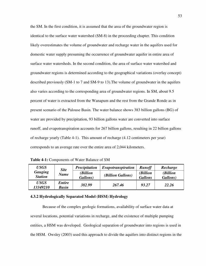
53

the SM. In the first condition, it is assumed that the area of the groundwater region is

identical to the surface water watershed (SM-8) in the proceeding chapter. This condition

likely overestimates the volume of groundwater and recharge water in the aquifers used for

domestic water supply presuming the occurrence of groundwater aquifer in entire area of

surface water watersheds. In the second condition, the area of surface water watershed and

groundwater regions is determined according to the geographical variations (overlay concept)

described previously (SM-1 to 7 and SM-9 to 13).The volume of groundwater in the aquifers

also varies according to the corresponding area of groundwater regions. In SM, about 9.5

percent of water is extracted from the Wanapum and the rest from the Grande Ronde as in

present scenario of the Palouse Basin. The water balance shows 383 billion gallons (BG) of

water are provided by precipitation, 93 billion gallons water are converted into surface

runoff, and evapotranspiration accounts for 267 billion gallons, resulting in 22 billion gallons

of recharge yearly (Table 4-1). This amount of recharge (4.12 centimeters per year)

corresponds to an average rate over the entire area of 2,044 kilometers.

Table 4-1: Components of Water Balance of SM

Precipitation Evapotranspiration Runoff Recharge USGS

Gauging

Station

Site

Name (Billion

Gallons) (Billion Gallons)

(Billion

Gallons

(Billion

Gallons)

USGS

13349210

Entire

Basin 382.99 267.46 93.27 22.26

4.3.2 Hydrologically Separated Model (HSM) Hydrology

Because of the complex geologic formations, availability of surface water data at

several locations, potential variations in recharge, and the existence of multiple pumping

entities, a HSM was developed. Geological separation of groundwater into regions is used in

the HSM. Owsley (2003) used this approach to divide the aquifers into distinct regions in the

54

Palouse Region. Figure 4-5 shows the schematic of the HSM.

Figure 4-5: Schematic of Connectivity in the HSM

The study of boundary conditions between the Moscow and Pullman groundwater

regions indicates that there can be boundary conditions between these cities (Sherman and

Osiensky, 2007). If the boundary condition exists between Moscow and Pullman, Pullman

can get water from west but Moscow has limited groundwater region to extract water

(Sherman and Osiensky, 2007). The aquifer test study (Moscow wells 2, 3, 6) of groundwater

monitoring and aquifer testing in the Wanapum aquifer showed the poor hydraulic

connection between the wells, and the Wanapum groundwater regions appears to be

compartmentalized (Bandon and Osiensky, 2007). Also, there is minimal flow between the

Palouse Basin above Colfax

USGS

13345000

USGS

13345300

USGS

13346100

N/A

South Fork

USGS

13346800

USGS

13348000

Wanapum

Palouse

Wanapum

Viola

Wanapum

Pullman

Wanapum

Moscow

Wanapum

Colfax

Grande Ronde

Colfax

Grande Ronde

Viola

Grande Ronde

Moscow

Grande Ronde

Pullman

Grande Ronde

Palouse

55

Pullman and Moscow aquifers (Leek, 2006). These arguments help to form the base of HSM

model. A basic assumption of this conceptualization is that the recharged water moves

vertically into groundwater regions in a spatially uniform manner within each region. In

addition, the groundwater regions receive different rates of recharged water. The water

balance was computed over each surface water watershed separately.

Table 4-2 shows the components of water balance of each surface water watershed in

terms of billion gallons. The Palouse groundwater region, overlaid by four surface water

watersheds, has the greatest variation in recharge rates while the Viola groundwater region

has the least. The Moscow groundwater region gets recharged from three different surface

watersheds while the Pullman groundwater region gets recharged from two. Because of the

geological formation and infrastructures, the potential groundwater drawdown of the

Moscow Grande Ronde and Pullman Grande Ronde aquifers are different.

Table 4-3 shows the initial volume of the groundwater in the Wanapum and Grande

Ronde computed by the potential groundwater drawdown at the bottom of the wells. This

computation uses the storativity value of 10-3. The groundwater volume of these aquifers will

be decreased by factor of 100 with lower storativity value (i.e., 10-5). The initial groundwater

volume of the Wanapum except Moscow is assumed to be zero. The volume of groundwater

in the aquifers was computed by Equation 3-2.

56

Table 4-2: Components of Water Balance of HSM

Precipitation Evapotranspiration Runoff Recharge USGS

Gauging Stations

Site Name

(Billion Gallons) (Billion Gallons) (Billion Gallons)

(Billion Gallons)

13345000 Palouse River near

Potlatch, ID 182.78 116.16 63.01 3.61

13345300 Palouse River at

Palouse, WA 12.30 8.57 0.89 2.84

13346100 Palouse River at

Colfax, WA (North Fork)

60.85 46.41 7.82 6.63

N/A South Fork Palouse above Colfax, WA

68.32 51.86 12.08 4.38

13346800 Paradise Creek at UI at

Moscow, ID 9.06 6.01 1.99 1.06

13348000 South Fork Palouse

River at Pullman, WA 49.69 35.12 7.63 6.94

Total 383 264.13 93.42 25.45

Table 4-3 shows the total initial volume of the Wanapum is about 1.6 billion gallons

when potential drawdown at the bottoms of the wells. In the similar condition, the Grande

Ronde has 40 billion gallons initial volume. The total groundwater volume computed from

average thickness (total depth) of aquifers is slightly larger than in the previous condition

(49.15 billion gallons; Table 4-3). The total volume of groundwater in the Wanapum and

Grande Ronde represents the total stored water in the aquifers irrespective to the present

water level. If no recharge in the aquifer is assumed, this groundwater volume represents the

total amount of groundwater in the Grande Ronde from its formation.

57

Table 4-3: Initial Volume of Groundwater in Aquifers

Groundwater

Area

Potential Groundwater Drawdown

at the bottom of wells

Average Thickness of

Aquifers

Groundwater Volume up to

bottom of wells

Total Groundwater

Volume (Total Depth)

Name

(km2)

Storativity

(meter) (meter) (Billion gallons)

(Billion gallons)

Wanapum

Moscow 81.75 10E-03 74 137.19 1.60 2.96

Total 1.60 2.96

Grande Ronde

Moscow 63.94 10E-03 271 259 4.58 4.58

Pullman 235.97 10E-03 161 305 10.04 19.01

Viola 21.25 10E-03 244 244 1.37 1.37

Palouse 74.32 10E-03 152 152 2.98 2.98

Colfax 332.13 10E-03 244 244 21.41 21.41

Total 40.37 49.15

Because of low storativity value (i.e., 10-3), the initial groundwater volumes are

smaller compared to the groundwater extraction. But conversely, Ralston (2004) mentioned

that the groundwater storage volume of these aquifers is still large (not quantified). It

basically indicates that the storativity value used in this study for calculating the initial

groundwater volume is to be further justified. The annual changes in water volume are

determined by the changes in groundwater level in aquifers. The groundwater level changes

in the wells are shown in Table 3-3 (pumping levels).

Table 4-4 shows the computation of recharge from different surface water sub-

watersheds to the corresponding groundwater regions of the upper aquifer, the Wanapum. It

is a portion of the surface water balance that reaches to the designated groundwater regions.

Computation of the surface water balance showed that out of 22 billion gallons of recharged

water; only 13 billion (about 60 percent) of water has reached to groundwater regions. Rest

40 percent recharged water is outside the groundwater regions and is not considered for

groundwater computation.

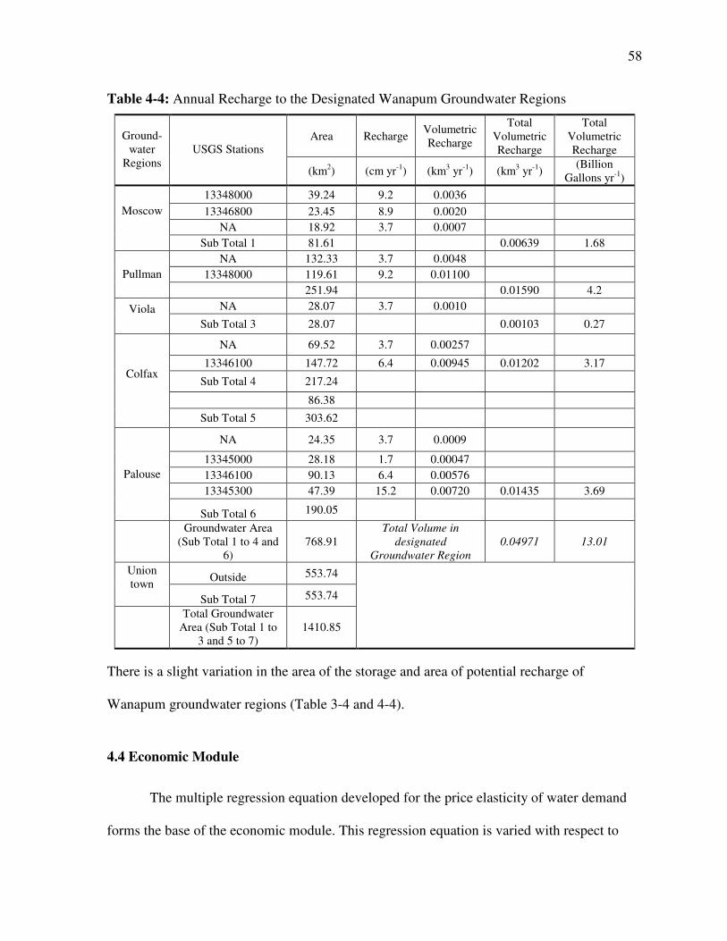
58

Table 4-4: Annual Recharge to the Designated Wanapum Groundwater Regions

Area Recharge Volumetric Recharge

Total Volumetric Recharge

Total Volumetric Recharge

Ground-water

Regions USGS Stations

(km2) (cm yr-1) (km3 yr-1) (km3 yr-1) (Billion

Gallons yr-1)

13348000 39.24 9.2 0.0036

13346800 23.45 8.9 0.0020

NA 18.92 3.7 0.0007

Moscow

Sub Total 1 81.61 0.00639 1.68

NA 132.33 3.7 0.0048

13348000 119.61 9.2 0.01100 Pullman

251.94 0.01590 4.2

NA 28.07 3.7 0.0010 Viola Sub Total 3 28.07 0.00103 0.27

NA 69.52 3.7 0.00257

13346100 147.72 6.4 0.00945 0.01202 3.17

Sub Total 4 217.24

86.38

Colfax

Sub Total 5 303.62

NA 24.35 3.7 0.0009

13345000 28.18 1.7 0.00047

13346100 90.13 6.4 0.00576

13345300 47.39 15.2 0.00720 0.01435 3.69

Palouse

Sub Total 6 190.05

Groundwater Area

(Sub Total 1 to 4 and 6)

768.91 Total Volume in

designated

Groundwater Region

0.04971 13.01

Outside 553.74 Union town

Sub Total 7 553.74

Total Groundwater Area (Sub Total 1 to

3 and 5 to 7) 1410.85

There is a slight variation in the area of the storage and area of potential recharge of

Wanapum groundwater regions (Table 3-4 and 4-4).

4.4 Economic Module

The multiple regression equation developed for the price elasticity of water demand

forms the base of the economic module. This regression equation is varied with respect to

59

time and water demand trend analysis is conducted. The trend of water demand can be

calculated by the economic module assuming the entire independent variables will behave in

a similar trend for certain period. Also the short term water demand analysis can be done by

increasing water price to decrease the water demand. The most important question here is to

compute the impact of change in water price to the water demand. Price elasticity relates

water demand to cost; in general, as cost increases, demand decreases.

Economic Scenario 1

In the Economic Scenario 1, regression analysis is carried out for single family user

class of City of Pullman. In Case 1, all five independent variables are used whereas in Case

2, the regression is carried out without household size. Results are shown in Table 4-5. In

Case 1, the result shows unrealistic results with large elasticity values in household size and

median household income. In both cases, the price elasticity of water demand has larger

value with positive sign. The coefficient of determination in both cases is 0.77. The negative

and positive signs in Table 4-5 and 4-6 are expected signs of variables in the regression

equations.

Table 4-5: Regression Coefficients for Price Elasticity Curve for Single Family

Marginal Price

Fixed Price

Median Household

Income

Household Size

Precipitation Constant Coefficient of Determination

F Statistics

MP FP I H P C R2 F

Expected signs of the variables

- - + + -

Case 1 General Case

2.97 -6.96 41.06 355.03 -0.09 153564.7 0.77 50.64

Case 2 General Case without household size

2.95 -7.18 5.82 -0.09 -33.89 0.77 63.52

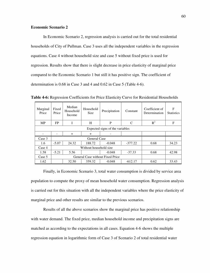
60

Economic Scenario 2

In Economic Scenario 2, regression analysis is carried out for the total residential

households of City of Pullman. Case 3 uses all the independent variables in the regression

equations. Case 4 without household size and case 5 without fixed price is used for

regression. Results show that there is slight decrease in price elasticity of marginal price

compared to the Economic Scenario 1 but still it has positive sign. The coefficient of

determination is 0.68 in Case 3 and 4 and 0.62 in Case 5 (Table 4-6).

Table 4-6: Regression Coefficients for Price Elasticity Curve for Residential Households

Marginal Price

Fixed Price

Median Household

Income

Household Size

Precipitation Constant Coefficient of Determination

F Statistics

MP FP I H P C R2 F

Expected signs of the variables

- - + + -

Case 3 General Case

1.6 -5.07 24.32 188.72 -0.048 -377.22 0.68 34.23

Case 4 Without household size

1.58 -5.21 5.56 -0.048 -37.33 0.68 42.98

Case 5 General Case without Fixed Price

1.62 32.50 359.32 -0.048 -612.17 0.62 33.43

Finally, in Economic Scenario 3, total water consumption is divided by service area

population to compute the proxy of mean household water consumption. Regression analysis

is carried out for this situation with all the independent variables where the price elasticity of

marginal price and other results are similar to the previous scenarios.

Results of all the above scenarios show the marginal price has positive relationship

with water demand. The fixed price, median household income and precipitation signs are

matched as according to the expectations in all cases. Equation 4-6 shows the multiple

regression equation in logarithmic form of Case 3 of Scenario 2 of total residential water

61

demand and Equation 4-7 in exponential form.

22.377)ln(

*048.0)ln(*72.188)ln(*32.24)ln(*07.5)ln(*6.1)ln(

−

−++−=

P

HIFPMPQ (4-6)

22.377048.072.18832.2407.56.1 ***** −−−= ePHIFPMPQ (4-7)

The marginal price elasticity of demand is +1.6, which means that 1 percent increase of water

price will increase water use by 1.6 percent. The price elasticity for fixed price is -5.07.

Water demand projected from the regression equation can be used to compute per

capita per day water use in designated years (Equation 4-8).

365*Pr

Pr

Populationojected

YearperDemandWaterojectedUseWaterDayperCapitaPer = (4-8)

Finally, forecasted per capita per day water use can be linked with the population model to

forecast water demand from the demand model.

4.5 Water Management Strategy

Both the SM and HSM are used to manage the water resources in the Palouse Basin.

The general trend of the total groundwater depletion in the aquifers can be visualized by the

SM whereas groundwater region wide trends by the HSM. The SM is used to evaluate the

water resources with the present infrastructures and the possible future infrastructures by

increasing potential groundwater drawdown. The primary attempt to manage water resources

in the Palouse Basin is to utilize groundwater sustainably. This is more challenging in the

Pullman area which solely depends in the lower aquifer; the Grande Ronde. So, the

management of water resources of the Pullman can be done either utilizing the groundwater

sustainably before the situation becomes worse or shifting to the surface water (or any other

feasible alternative options). The existence of the upper aquifer, the Wanapum, provides one

62

more options to manage the Moscow water resources. PBAC has also mentioned that the

shallow aquifer (Wanapum) in the Moscow can be used to reduce pumping pressure on the

deep aquifer (Grande Ronde). Additionally, the Wanapum can also be used to increase

recharge of the Grande Ronde (PBAC, 2004).

4.5.1 HSM for Water Resource Management with Current Infrastructures

This section discusses the use of HSM to evaluate the water resources situation of the

Palouse Basin with current infrastructures. The existence of upper and lower aquifers in the

Moscow region has increased possibility of future water management options of this area. At

present, 68 percent of domestic water in Moscow is extracted from the Grande Ronde and 32

percent from the Wanapum (PBAC, 2006). Within the present infrastructures condition,

when the Moscow Grande Ronde reaches to certain minimum volume, then the alternative is

shifting to the Wanapum but the Pullman doesn’t have this choice. Minimum Volume

Grande Ronde represents the minimum amount of water that is always stored in Grande

Ronde aquifer.

a) Moscow Groundwater Management Strategy

If volume of groundwater in the Moscow Grande Ronde reaches a certain minimum

volume, then water demand will be fulfilled by Moscow Wanapum. Otherwise thirty percent

of Moscow water demand is fulfilled by Wanapum and seventy percent of water is fulfilled

by Grande Ronde (Equation 4-9 and 4-10).

)*3.0()(

)(

DemandMoscowElseDemandMoscowthen

VolumeMinimumRondeGrandeMoscowIfWanapumMoscow <= (4-9)

)*7.0( DemandMoscowRondeGrandeMoscow = (4-10)

This condition reflects the current water management situation of the Moscow.

63

b) Pullman Groundwater Management Strategy

If volume of groundwater in the Pullman Grande Ronde reaches a certain minimum

volume, then alternative sources will have to be fetched. Otherwise hundred percent of water

is fulfilled by Pullman Grande Ronde (Equation 4-11).

)()0(

)(

DemandPullmanElsethen

VolumeMinimumRondeGrandePullmanIfRondeGrandePullman <= (4-11)

This management strategy reflects the present water management situation of the Pullman.

4.5.2 HSM for Water Resource Management with Surface Water Utilization

WRIA-34 identifies diverted stream flow, shallow groundwater, reclaimed water,

storm water and precipitation as potential water resources of this basin. Many other studies

also mentioned the use of surface water for solving water problems of the Palouse Basin.

This section discusses the water demand management of the Moscow and Pullman by

utilizing surface water.

Surface Water Utilization Module

A promising alternative to manage water resource in the Palouse Basin is the

combined use of groundwater and surface water (Stevens, 1970; Fealko, 2003; WRIA-34,

2004). The surface water from the Paradise Creek and South Fork of the Palouse River can

be utilized (PBAC, 2004). The Surface Water Utilization Module is used to evaluate

potential use of surface water in the basin. In this version of the module, it is assumed that

overall eight percent of the surface water has the potential to be utilized. The future model

development will address actual water rights and ecological needs, thus reducing the amount

of available surface water. The surface water utilization will open numerous water

management strategies in this watershed. One of the probable water management strategies

64

of the Moscow and Pullman is discussed below. The general condition here means the

condition before the Grande Ronde reaches minimum volume which can’t be extracted.

a) Moscow Groundwater Management Strategy

If volume of groundwater in the Moscow Grande Ronde reaches a certain minimum

volume, then fifty percent of the water demand will be fulfilled by Moscow Wanapum and

the remaining fifty percent by surface water. In general condition, thirty percent of the water

demand is to be fulfilled by Moscow Wanapum, another twenty-five percent by Moscow

Grande Ronde and the remaining forty-five percent by Moscow surface water (Equation 4-

12, 4-13 and 4-14).

)*25.0()0(

)(

DemandMoscowElsethen

VolumeMinimumRondeGrandeMoscowIfRondeGrandeMoscow <= (4-12)

)*3.0()*5.0(

)(


VolumeMinimumRondeGrandeMoscowIfWanapumMoscow <= (4-13)

)*45.0()*5.0(

)(


VolumeMinimumRondeGrandeMoscowIfWaterSurfaceMoscow <= (4-14)

b) Pullman Groundwater Management Strategy

If volume of groundwater in Pullman Grande Ronde reaches a certain minimum

volume, then hundred percent of the water demand will be fulfilled by Pullman surface

water. In general condition, fifty percent of the demand is to be fulfilled by Pullman Grande

Ronde and the remaining fifty percent by Pullman surface water (Equation 4-15 and 4-16).

)*5.0()0(

)(

DemandPullmanElsethen

VolumeMinimumRondeGrandePullmanIfRondeGrandePullman <= (4-15)

)*5.0()(

)(

DemandPullmanElseDemandPullmanthen

VolumeMinimumRondeGrandePullmanIfWaterSurfacePullman <= (4-16)

65

In Pullman, the dependency on Grande Ronde water can be reduced by 50 percent

replacing with the surface water.

4.6 Sustainability Index (SI)

It is difficult to define the overall sustainability of water resources of the Palouse

Basin, given that the components like environmental and legal factors are not included in this

research. Sustainability of water resources with surface and groundwater (discussed in the

previous sections) is still difficult because of the limited study of the surface water. So

sustainability of the groundwater is presented in the limited boundary of the annual

extraction and recharge pattern. The unique geology and water extraction pattern of the

Palouse Region makes the sustainability study of the water resources still challenging.

Because of the complex geologic formation, the recharged water reaches to the upper aquifer,

Wanapum. The uncertainty of the possible interconnection between the upper aquifer,

Wanapum and the lower aquifer, Grande Ronde, is another equally important issue. In a

general perspective, assuming water balance is correct, the annual recharge rate is greater

than the extraction rate in the Palouse Basin watershed. But the entire Palouse Basin is

dependent on the lower aquifer, Grande Ronde which has essentially no recharge. So the

sustainability of the Grande Ronde is more important in our context. Some probabilistic

scenarios to evaluate the sustainability of the basin are discussed below. To be consistent to

the groundwater indicators by UNESCO, the groundwater SI of both the Wanapum and

Grande Ronde are calculated from Equation 4-17 and 4-18 respectively.

%100*WANAPUM

WANAPUMTGR

TGAGSI

= (4-17)

GSI of Wanapum is basically the ratio of total recharged water to designated

66

groundwater regions of the Wanapum to the total water extraction.

%100*RONDEGRANDE

RONDEGRANDETGR

TGAGSI

= (4-18)

Groundwater Sustainability Index (GSI) of the Grande Ronde basically is the ratio of

the recharged water to the Grande Ronde to the total water demand. Total recharged water to

the Grande Ronde is the summation of recharged water to five groundwater regions annually.

Total demand is the summation of annual water demand of aforementioned cities. A

challenge here is to understand the water recharge pattern to the Grande Ronde. The

sustainability of the Grande Ronde not only depends on the present recharge and extraction

but also to the initial volume of groundwater in the aquifer. Many water scientists believe

that the recharge to the Grande Ronde is negligible and it is further justified that the age of

the groundwater of the Grande Ronde is more than 10,000 years ago. For sustainability of

groundwater systems, the annual recharge should balance extraction rate. If we assume no

recharge to the Grande Ronde, then from basic definition, groundwater to the Grande Ronde

is unsustainable. So if assumed no recharge to the Grande Ronde, the key question becomes

how many more years this aquifer will last in current water use pattern.

An important argument here is the total recharge water that enters in the Wanapum

has very small water demand. Conversely, the total water demand of the Palouse Basin is

fulfilled by the Grande Ronde which has literally no recharge. So GSI of the Wanapum

shows the overall sustainability of groundwater. At the same time, GSI of the Grande Ronde

shows the sustainability of Grande Ronde aquifer. So they both have particular importance in

defining sustainability of groundwater this region.

67

CHAPTER V

RESULTS AND DISCUSSION

5.0 Overview

In this chapter, the results of simulations are presented, and key parameters are

varied. Sensitivity analyses are carried out by varying storativity, recharge and area of

groundwater regions. An annual time interval was used for simulation. The population of this

area is estimated to grow by 1 percent annually (PBAC, 2000). The per capita per day water

use of the Palouse Basin is taken as 160 gallons (PBAC, 2000). All volumetric components

of the models are characterized in billion gallons. Simulations are carried out using SM and

HSM for the present infrastructure conditions and the probable future extension possibilities.

5.1 Domestic Water Demand

The Grande Ronde has comparatively small recharge with much higher water

extraction rate than the Wanapum. Total water extraction from the Palouse Basin is 2.77

billion gallons in the year 2005 (PBAC, 2005). Approximately 9.5 percent of the total water

demand of the Palouse Basin is fulfilled by the Wanapum and rest by the Grande Ronde.

Water extraction from the Grande Ronde (2.51 billon gallons per year) is approximately nine

times greater than the Wanapum (0.26 billon gallons per year) in the year 2005.

The water demand model estimates 2.97 billion gallons annual water demand of the

Palouse Basin at 2005 and will be about 7.63 billion gallons after one hundred years. The

projected population of the Palouse is about 139,073 people after one hundred years which is

approximately three times of the present population. Figure 5-1 shows the water demand

projection of the Palouse Basin with 1 percent annual growth rate. There is a small variation

in exact water extraction and modeled values which is because of the discrepancies on the

68

population growth rate, per capita per day water consumption and the yearly population data.

0

1.5

3

4.5

6

7.5

9

20042020

20362052

20682084

2100

Years

Wa

ter

Dem

an

d (

Bil

lio

n G

all

on

s)

Figure 5-1: Water Demand Projection of the Palouse Basin

0

1

2

3

4

20052021

20372053

20692085

Year

Wa

ter

Dem

an

d (

Billio

n G

allo

ns)

Moscow

Demand

Colfax

Demand

Pullman

Demand

Figure 5-2: Water Demand Projection of the Major Cities

Figure 5-2 shows water demand projection of the aforementioned cities of the Palouse

Basin. The estimated demand in the initial year (2005) is 0.16 billion gallons for Colfax, 1.27

69

billion gallons for Moscow, 0.04 billion gallons for Potlatch, 0.02 billion gallons for Viola

and 1.47 billion gallons for Pullman. The exact water extraction figures in the year 2005

from these cities are 1.05, 1.38 and 0.266 billion gallons by Moscow, Pullman and Colfax

respectively. The increase in commercial and industrial activities may further increase the

demand of water.

5.2 Simple Model (SM)

Basically, SM is a lumped model in which the Wanapum and Grande Ronde aquifers

act as single units. SM is used to evaluate the present water practice and as future indicator.

No specific management strategy is discussed except the possibility of increasing potential

groundwater drawdown by lowering the pumps. Altogether 13 scenarios shown on Table 5-1

are presented in this section. Scenarios 1 to 6 discuss the current and future infrastructure

conditions with varying potential groundwater drawdown. Scenarios 1 and 2 discuss the

potential groundwater drawdown at the bottom of the pump whereas scenarios 3 to 6 to the

bottom of the wells. The depth of the bottom of pumps of Colfax, Viola and Palouse region

are assumed to be identical to Pullman Region. Scenario 7 discusses the situation if the

potential recharge area of the Wanapum is identical to the Moscow groundwater region.

Contrary to Scenario 7, Scenario 8 address the impact of increase in surface area of

groundwater region assuming the entire surface water watershed has the potential for

recharge. Scenarios 9 to 10 discuss the groundwater situation from back calculated storativity

values. Scenarios 11 to 13 discuss an attempt to simulate the present groundwater level trend

of the Wanapum aquifer.

70

Table 5-1 : SM Applied Conditions

Potential groundwater drawdown

Groundwater region areas

Recharge Initial Volume

Grande Ronde Wanapum Moscow

Moscow Pullman WP GR WP GR WP GR

Scenario

(m) (km2) (cm yr-1) (BG yr-1 )

Storativity

1 2 3 4 5 6 7 8 9 10 11

SM-1 30 34 51 769 769 6.4 0 0.06 0.95 0.0001

SM-2 30 34 51 769 769 6.4 0 0.57 9.5 0.001

SM-3 74 271 161 769 769 6.4 0 0.16 4.26 0.0001

SM-4 74 271 161 769 769 6.4 0 1.61 42.64 0.001

SM-5 74 271 161 769 769 6.4 1 1.61 42.64 0.001

SM-6 74 271 161 769 769 6.4 2 1.61 42.64 0.001

SM-7 74 271 161 81.61 769 7.79 0 1.61 42.64 0.001

SM-8 74 271 161 2,044 2,044 4.12 0 40.16 146.49 0.001

SM-9 30 34 51 769 769 6.4 0 16.7 281.62 0.03

SM-10 74 271 161 769 769 6.4 0 47.2 1257.7 0.03

SM-11 30 34 51 769 769 0.34 0 0.57 9.5 0.001

SM-12 30 34 51 769 769 0.34 0 16.7 281.62 0.03

SM-13 74 271 161 769 769 0.22 0 47.2 1257.7 0.03

Column 10 of the Table 5-1 shows the initial volume of the groundwater in the

Grande Ronde is 0.95 and 9.5 billion gallons in Scenario 1 and 2 respectively. In the no

recharge assumption, these initial volumes represent the total volume of groundwater to the

Grande Ronde. From the year 1964 to date, more than 70 billion gallons water was extracted

from the Pullman and Moscow Grande Ronde only. As in scenarios 1 to 7, no recharge to the

Grande Ronde with current infrastructure (storativity of 10-3 to 10-5, groundwater drawdown

of 30-40m and area of 769 square kilometers), the total amount of water in the Grande Ronde

is smaller than the water extracted. In Scenario 7, the total recharge to the Wanapum is

assumed to be equal to the Moscow recharge. The initial volume of the Wanapum in this

scenario will be similar to other scenarios because potential groundwater drawdown of other

groundwater regions (i.e., Pullman, Colfax, Palouse and Viola) is assumed to be zero. All the

above scenarios except 8 have Grande Ronde aquifer area of 769 square kilometers.

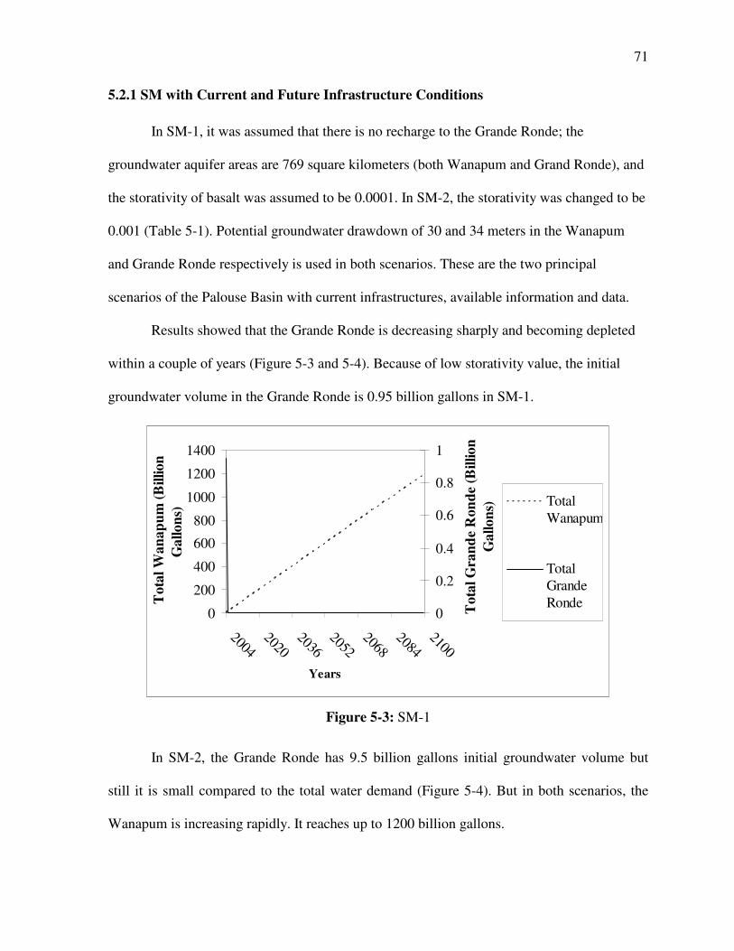
71

5.2.1 SM with Current and Future Infrastructure Conditions

In SM-1, it was assumed that there is no recharge to the Grande Ronde; the

groundwater aquifer areas are 769 square kilometers (both Wanapum and Grand Ronde), and

the storativity of basalt was assumed to be 0.0001. In SM-2, the storativity was changed to be

0.001 (Table 5-1). Potential groundwater drawdown of 30 and 34 meters in the Wanapum

and Grande Ronde respectively is used in both scenarios. These are the two principal

scenarios of the Palouse Basin with current infrastructures, available information and data.

Results showed that the Grande Ronde is decreasing sharply and becoming depleted

within a couple of years (Figure 5-3 and 5-4). Because of low storativity value, the initial

groundwater volume in the Grande Ronde is 0.95 billion gallons in SM-1.

0

200

400

600

800

1000

1200

1400

20042020

20362052

20682084

2100

Years

To

tal

Wa

na

pu

m (

Billio

n

Ga

llo

ns)

0

0.2

0.4

0.6

0.8

1

To

tal

Gra

nd

e R

on

de

(Billio

n

Ga

llo

ns) Total

Wanapum

TotalGrande

Ronde

Figure 5-3: SM-1

In SM-2, the Grande Ronde has 9.5 billion gallons initial groundwater volume but

still it is small compared to the total water demand (Figure 5-4). But in both scenarios, the

Wanapum is increasing rapidly. It reaches up to 1200 billion gallons.

72

0

200

400

600

800

1000

1200

1400

20042020

20362052

20682084

2100

Years

To

tal

Wa

na

pu

m (

Billio

n

Ga

llo

ns)

0

2

4

6

8

10

12

To

tal

Gra

nd

e R

on

de

(Billio

n

Ga

llo

ns)

Total

Wanapum

Total

GrandeRonde

Figure 5-4: SM-2

Simulations assuming water level depletion in the Grande Ronde aquifer to the

bottom of the wells (Scenario 3 and 4) were also conducted. Even if the potential

groundwater drawdown is increased, the Grande Ronde has a sharp decline (Figure 5-5 and

5-6).

0

200

400

600

800

1000

1200

1400

20042020

20362052

20682084

2100

Years

To

tal

Wa

na

pu

m (

Billio

n

Ga

llo

ns)

0

0.5

1

1.5

2

2.5

3

3.5

4

4.5

To

tal

Gra

nd

e R

on

de

(Billio

n

Ga

llo

ns) Total

Wanapum

TotalGrande

Ronde

Figure 5-5: SM-3

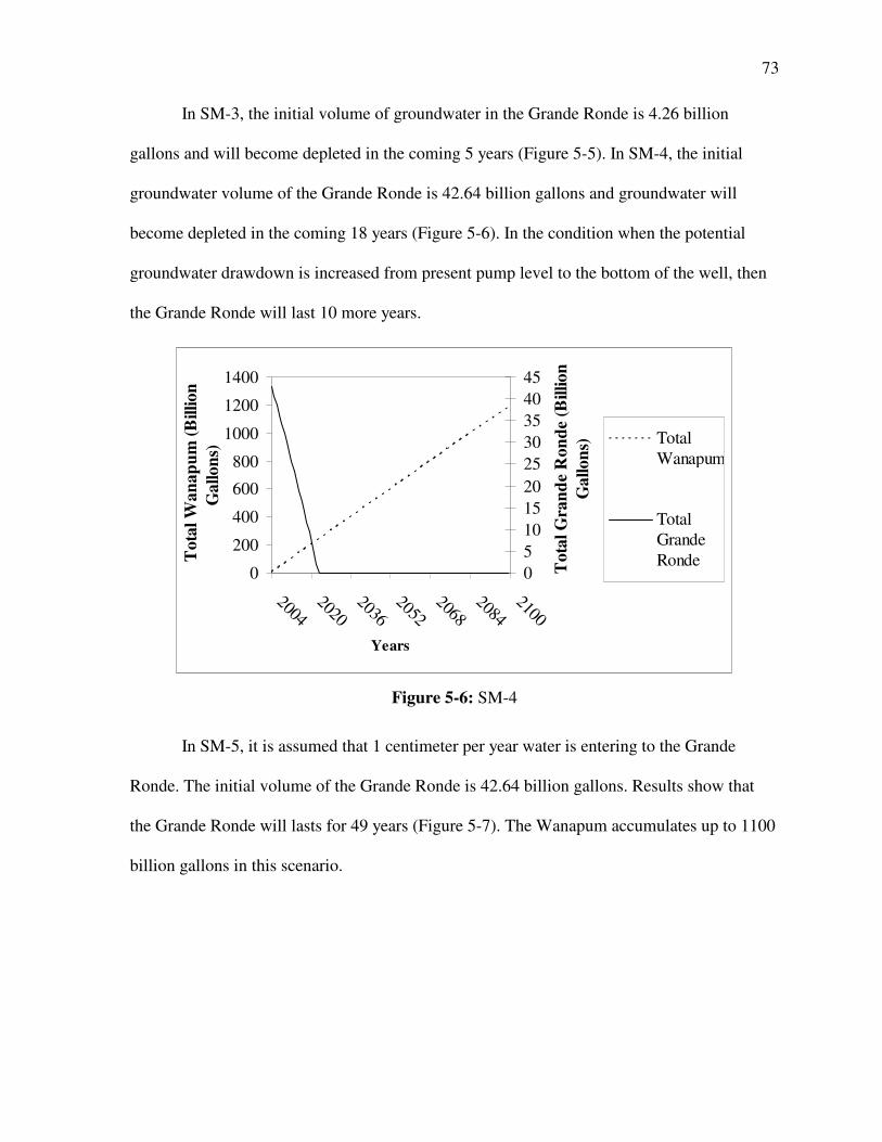
73

In SM-3, the initial volume of groundwater in the Grande Ronde is 4.26 billion

gallons and will become depleted in the coming 5 years (Figure 5-5). In SM-4, the initial

groundwater volume of the Grande Ronde is 42.64 billion gallons and groundwater will

become depleted in the coming 18 years (Figure 5-6). In the condition when the potential

groundwater drawdown is increased from present pump level to the bottom of the well, then

the Grande Ronde will last 10 more years.

0

200

400

600

800

1000

1200

1400

20042020

20362052

20682084

2100

Years

To

tal

Wa

na

pu

m (

Billio

n

Ga

llo

ns)

0

5

10

15

20

25

30

35

40

45

To

tal

Gra

nd

e R

on

de

(Billio

n

Ga

llo

ns) Total

Wanapum

TotalGrande

Ronde

Figure 5-6: SM-4

In SM-5, it is assumed that 1 centimeter per year water is entering to the Grande

Ronde. The initial volume of the Grande Ronde is 42.64 billion gallons. Results show that

the Grande Ronde will lasts for 49 years (Figure 5-7). The Wanapum accumulates up to 1100

billion gallons in this scenario.

74

0

200

400

600

800

1000

1200

20042020

20362052

20682084

2100

Years

To

tal

Wa

na

pu

m (

Billio

n

Ga

llo

ns)

0

5

10

15

20

25

30

35

40

45

To

tal

Gra

nd

e R

on

de

(Billio

n

Ga

llo

ns) Total

Wanapum

TotalGrande

Ronde

Figure 5-7: SM-5

The groundwater depletion rate is about 4 to 24 feet per year which is much faster

when compared to the present trend (Figure 5-8).

0

150

300

450

600

750

20042020

20362052

20682084

2100

Years

Gra

nd

e R

on

de

(Fee

t)

Figure 5-8: SM-5 (Feet)

In SM-6, the recharge rate to the Grande Ronde is increased to 2 centimeters per year.

In the applied infrastructure condition, there is no change in the initial groundwater volume

75

in the Grande Ronde (42.64 billion gallons). But in contrary to the previous simulations, the

Grande Ronde has an increasing trend and accumulates up to 100 billion gallons in the

coming 70 years and reaches zero after 124 years (Figure 5-9). If there is a further increase in

the recharge rate to the Grande Ronde, the water level increases and it will be in rising trend.

0

200

400

600

800

1000

1200

1400

20042030

20562082

21082134

Years

To

tal

Wa

na

pu

m (

Billio

n

Ga

llo

ns)

0

20

40

60

80

100

120

To

tal

Gra

nd

e R

on

de

(Billio

n

Ga

llo

ns) Total

Wanapum

TotalGrande

Ronde

Figure 5-9: SM-6

Even if these principle scenarios (except Scenario 6) are indicating the groundwater

of the Grande Ronde lasts not more than 50 years and water level to the Wanapum rises up to

1200 billion gallons, the water level of both Grande Ronde and Wanapum is not realistic

when compared to the present trend. All the above scenarios show the water level is

depleting in an alarming rate (3 to 25 foot per year). So, further alternative scenarios will be

discussed in the coming sections.

5.2.2 Recharge Area of the Wanapum as Moscow Groundwater Region

In SM-7, the potential recharge area of the Wanapum is assumed to be identical to the

Moscow groundwater region. In the previous sections, the entire basalt area (769 square

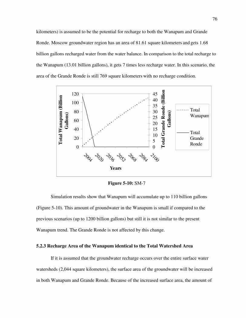
76

kilometers) is assumed to be the potential for recharge to both the Wanapum and Grande

Ronde. Moscow groundwater region has an area of 81.61 square kilometers and gets 1.68

billion gallons recharged water from the water balance. In comparison to the total recharge to

the Wanapum (13.01 billion gallons), it gets 7 times less recharge water. In this scenario, the

area of the Grande Ronde is still 769 square kilometers with no recharge condition.

0

20

40

60

80

100

120

20042020

20362052

20682084

2100

Years

To

tal

Wa

na

pu

m (

Billio

n

Ga

llo

ns)

0

5

10

15

20

2530

35

40

45

To

tal

Gra

nd

e R

on

de

(Billio

n

Ga

llo

ns)

Total

Wanapum

Total

GrandeRonde

Figure 5-10: SM-7

Simulation results show that Wanapum will accumulate up to 110 billion gallons

(Figure 5-10). This amount of groundwater in the Wanapum is small if compared to the

previous scenarios (up to 1200 billion gallons) but still it is not similar to the present

Wanapum trend. The Grande Ronde is not affected by this change.

5.2.3 Recharge Area of the Wanapum identical to the Total Watershed Area

If it is assumed that the groundwater recharge occurs over the entire surface water

watersheds (2,044 square kilometers), the surface area of the groundwater will be increased

in both Wanapum and Grande Ronde. Because of the increased surface area, the amount of

77

recharged water in the Wanapum will increase. But in the Grande Ronde, both recharge and

initial groundwater increases. In all the above discussed scenarios with no recharge to the

Grande Ronde, it is decreasing in an alarming rate. In this SM-8, the initial groundwater

volume of the Grande Ronde is 146.49 billion gallons.

0

500

1000

1500

2000

2500

20042020

20362052

20682084

2100

Years

To

tal

Wa

na

pu

m (

Billio

n

Ga

llo

ns)

0

20

40

60

80

100

120

140

160

To

tal

Gra

nd

e R

on

de

(Billio

n

Ga

llo

ns)

Total

Wanapum

Total

GrandeRonde

Figure 5-11: SM-8

Simulation results show the water level declination of the Grande Ronde aquifer is

milder than compared to the previous scenarios.

78

0

150

300

450

600

750

900

1050

20042020

20362052

20682084

2100

Years

Gra

nd

e R

on

de

(Fee

t)


Figure 5-12 shows an annual water level depletion of the Grande Ronde in feet. The

groundwater depletion rate is about 10 to 20 feet per year which is much faster when

compared to the present trend. An important question here is why is the water level from the

Grande Ronde declining in a much faster rate than the historic and present trend? The key

factors are storativity and recharge.

5.2.4 SM with Back Calculated Storativity

From the above discussion, either recharge or storativity values are apparently not in

the realistic range. So storativity was re-calculated in this section with an assumption of no

discharge and no recharge to the Grande Ronde, and it acts as a single unit. A constant water

level decline of 1.5 feet of entire Grand Ronde with an annual water extraction of 2.45 billion

gallons (PBAC, 2005) with the groundwater area of 769 square kilometers, the calculated

value of storativity value is 0.03. This value of storativity is approximately 30 times larger

than lower storativity value reported by Osiensky (2005). In SM-9, potential drawdown with

79

the current infrastructure is simulated whereas in SM-10 with future extension possibilities

from back calculated storativity. Results show that the initial volume of the groundwater in

the Grande Ronde is about 282 and 1258 billion gallons in SM-9 and SM-10 respectively

(Figure 5-13 and 5-14).

0

200

400

600

800

1000

1200

1400

20042020

20362052

20682084

2100

Years

To

tal

Wa

na

pu

m (

Billio

n

Ga

llo

ns)

0

50

100

150

200

250

300

To

tal

Gra

nd

e R

on

de

(Billio

n

Ga

llo

ns) Total

Wanapum

TotalGrande

Ronde

Figure 5-13: SM-9

Simulation results show that the Grande Ronde lasts for 84 years in SM-9 (Figure 5-

13).

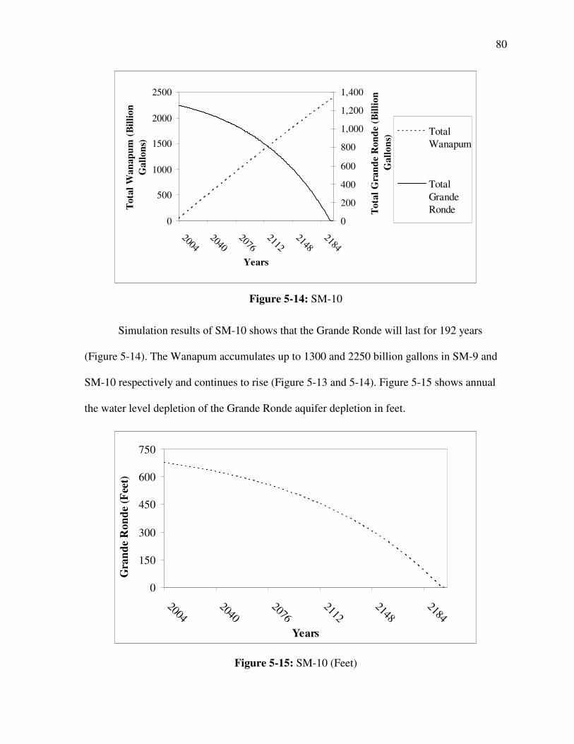
80

0

500

1000

1500

2000

2500

20042040

20762112

21482184

Years

Tota

l W

an

ap

um

(B

illi

on

Ga

llo

ns)

0

200

400

600

800

1,000

1,200

1,400

To

tal

Gra

nd

e R

on

de

(Bil

lio

n

Ga

llo

ns)

Total

Wanapum

Total

Grande

Ronde

Figure 5-14: SM-10

Simulation results of SM-10 shows that the Grande Ronde will last for 192 years

(Figure 5-14). The Wanapum accumulates up to 1300 and 2250 billion gallons in SM-9 and

SM-10 respectively and continues to rise (Figure 5-13 and 5-14). Figure 5-15 shows annual

the water level depletion of the Grande Ronde aquifer depletion in feet.

0

150

300

450

600

750

20042040

20762112

21482184

Years

Gra

nd

e R

on

de

(Fee

t)


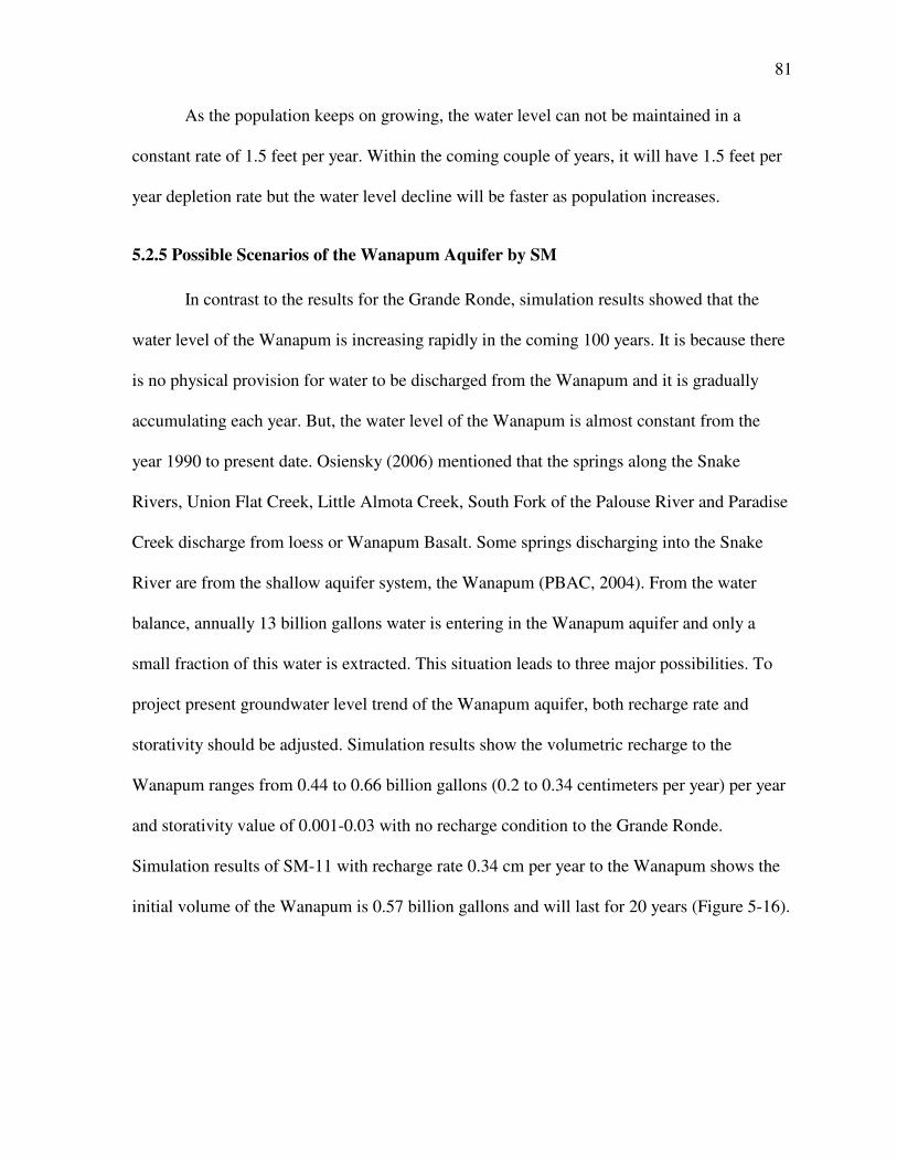
81

As the population keeps on growing, the water level can not be maintained in a

constant rate of 1.5 feet per year. Within the coming couple of years, it will have 1.5 feet per

year depletion rate but the water level decline will be faster as population increases.

5.2.5 Possible Scenarios of the Wanapum Aquifer by SM

In contrast to the results for the Grande Ronde, simulation results showed that the

water level of the Wanapum is increasing rapidly in the coming 100 years. It is because there

is no physical provision for water to be discharged from the Wanapum and it is gradually

accumulating each year. But, the water level of the Wanapum is almost constant from the

year 1990 to present date. Osiensky (2006) mentioned that the springs along the Snake

Rivers, Union Flat Creek, Little Almota Creek, South Fork of the Palouse River and Paradise

Creek discharge from loess or Wanapum Basalt. Some springs discharging into the Snake

River are from the shallow aquifer system, the Wanapum (PBAC, 2004). From the water

balance, annually 13 billion gallons water is entering in the Wanapum aquifer and only a

small fraction of this water is extracted. This situation leads to three major possibilities. To

project present groundwater level trend of the Wanapum aquifer, both recharge rate and

storativity should be adjusted. Simulation results show the volumetric recharge to the

Wanapum ranges from 0.44 to 0.66 billion gallons (0.2 to 0.34 centimeters per year) per year

and storativity value of 0.001-0.03 with no recharge condition to the Grande Ronde.

Simulation results of SM-11 with recharge rate 0.34 cm per year to the Wanapum shows the

initial volume of the Wanapum is 0.57 billion gallons and will last for 20 years (Figure 5-16).

82

0

0.1

0.2

0.3

0.4

0.5

0.6

20042014

20242034

2044

Years

To

tal

Wan

ap

um

(B

illi

on

Ga

llo

ns)

0

2

4

6

8

10

12

Tota

l G

ran

de

Ro

nd

e (B

illi

on

Ga

llon

s)

Total

Wanapum

Total

Grande

Ronde

Figure 5-16: SM-11

The adjusted volumetric recharge to the Wanapum is about 0.66 billion gallons with

storativity of 0.001. In SM-12, the initial volume of groundwater in the Wanapum is 16.7

billion gallons and will last for 90 years. The initial volume of the Grande Ronde is 281.62

billion gallons and will last 84 years (Figure 5-17).

0

2

4

6

8

10

12

14

16

18

20042020

20362052

20682084

2100

Years

To

tal

Wan

ap

um

(B

illi

on

Ga

llo

ns)

0

50

100

150

200

250

300

Tota

l G

ran

de

Ro

nd

e (B

illi

on

Ga

llon

s)

Total

Wanapum

Total

Grande

Ronde

Figure 5-17: SM-12

83

0

5

10

15

20

25

30

35

40

45

50

20042040

20762112

21482184

Years

To

tal

Wan

ap

um

(B

illi

on

Ga

llo

ns)

0

200

400

600

800

1,000

1,200

1,400

Tota

l G

ran

de

Ro

nd

e (B

illi

on

Ga

llon

s)

Total

Wanapum

Total

Grande

Ronde

Figure 5-18: SM-13

In SM-13, the rate of groundwater depletion in the Wanapum is almost constant but

because of gradual increase in population, it is becoming depleted in the coming 100 years.

The initial volume of groundwater in the Wanapum is 47.2 billion gallons and lasts

for 138 years in SM-13 (Figure 5-18). In this scenario, the total water level drop is only about

26 feet in the Wanapum aquifer in the coming 140 years whereas the Grande Ronde has 650

feet in the coming 180 years (Figure 5-19).

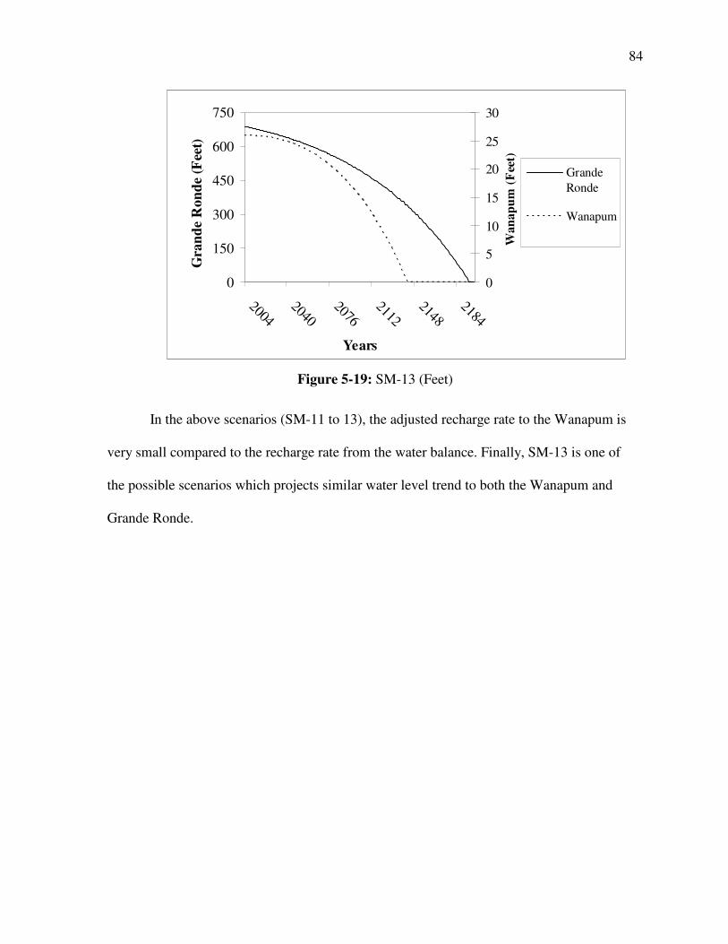
84

0

150

300

450

600

750

20042040

20762112

21482184

Years

Gra

nd

e R

on

de

(Fee

t)

0

5

10

15

20

25

30

Wan

ap

um

(F

eet)

Grande

Ronde

Wanapum


In the above scenarios (SM-11 to 13), the adjusted recharge rate to the Wanapum is

very small compared to the recharge rate from the water balance. Finally, SM-13 is one of

the possible scenarios which projects similar water level trend to both the Wanapum and

Grande Ronde.

85

Figure 5-20: Wanapum Water Level Trend (Ralston, 2004)

Figure 5-20 shows a gradual decrease of water level from 1940 to 1960s and recovery

of water level from 1960 to 1990s in two Wanapum wells. Ralston (2004) mentioned that the

water level of the Wanapum aquifer (at year 2004) is similar to 1940’s level (i.e., at the

beginning without water level drop). So, the water level depletion and recovery pattern of the

Wanapum aquifer indicates the effective recharge rate to the Wanapum is likely to be lower

than current water balance estimates. As in history, water level of the Wanapum has depleted

about 80 feet within 30 years (Figure 5-20), so it is not out of risk if more water is extracted.

5.2.6 Life of Groundwater Aquifers

Table 5-2 shows that within applied conditions, the maximum life of the Grande

Ronde is 192 years. SM-10 with back calculated storativity projects longest life period. This

is an optimistic scenario because the storativity value is relatively high compared to the

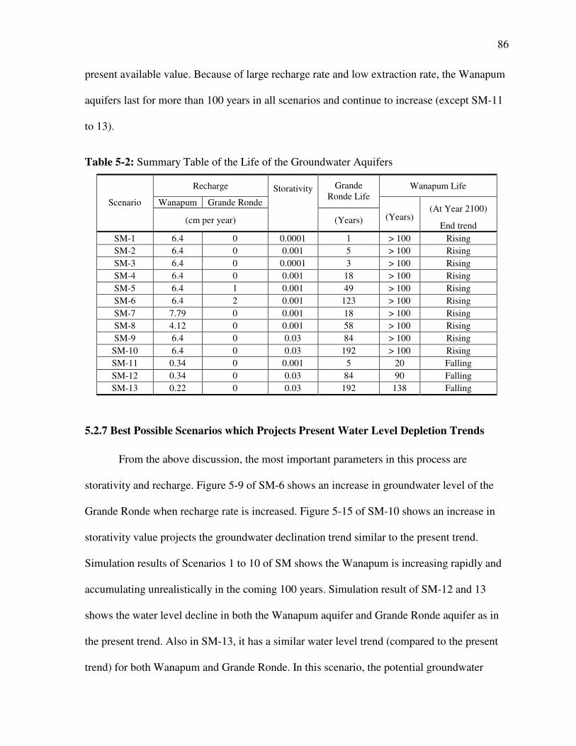
86

present available value. Because of large recharge rate and low extraction rate, the Wanapum

aquifers last for more than 100 years in all scenarios and continue to increase (except SM-11

to 13).

Table 5-2: Summary Table of the Life of the Groundwater Aquifers

Recharge Wanapum Life

Wanapum Grande Ronde

Grande Ronde Life

Scenario

(cm per year)

Storativity

(Years) (Years) (At Year 2100)

End trend

SM-1 6.4 0 0.0001 1 > 100 Rising

SM-2 6.4 0 0.001 5 > 100 Rising

SM-3 6.4 0 0.0001 3 > 100 Rising

SM-4 6.4 0 0.001 18 > 100 Rising

SM-5 6.4 1 0.001 49 > 100 Rising

SM-6 6.4 2 0.001 123 > 100 Rising

SM-7 7.79 0 0.001 18 > 100 Rising

SM-8 4.12 0 0.001 58 > 100 Rising

SM-9 6.4 0 0.03 84 > 100 Rising

SM-10 6.4 0 0.03 192 > 100 Rising

SM-11 0.34 0 0.001 5 20 Falling

SM-12 0.34 0 0.03 84 90 Falling

SM-13 0.22 0 0.03 192 138 Falling

5.2.7 Best Possible Scenarios which Projects Present Water Level Depletion Trends

From the above discussion, the most important parameters in this process are

storativity and recharge. Figure 5-9 of SM-6 shows an increase in groundwater level of the

Grande Ronde when recharge rate is increased. Figure 5-15 of SM-10 shows an increase in

storativity value projects the groundwater declination trend similar to the present trend.

Simulation results of Scenarios 1 to 10 of SM shows the Wanapum is increasing rapidly and

accumulating unrealistically in the coming 100 years. Simulation result of SM-12 and 13

shows the water level decline in both the Wanapum aquifer and Grande Ronde aquifer as in

the present trend. Also in SM-13, it has a similar water level trend (compared to the present

trend) for both Wanapum and Grande Ronde. In this scenario, the potential groundwater

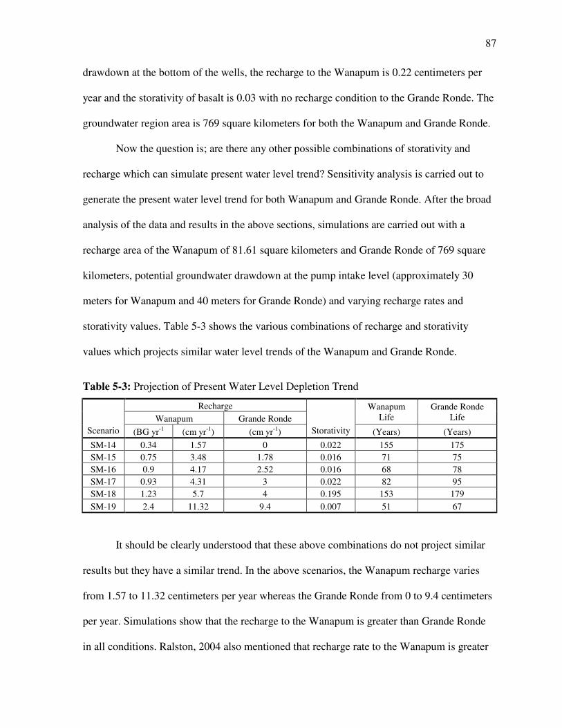
87

drawdown at the bottom of the wells, the recharge to the Wanapum is 0.22 centimeters per

year and the storativity of basalt is 0.03 with no recharge condition to the Grande Ronde. The

groundwater region area is 769 square kilometers for both the Wanapum and Grande Ronde.

Now the question is; are there any other possible combinations of storativity and

recharge which can simulate present water level trend? Sensitivity analysis is carried out to

generate the present water level trend for both Wanapum and Grande Ronde. After the broad

analysis of the data and results in the above sections, simulations are carried out with a

recharge area of the Wanapum of 81.61 square kilometers and Grande Ronde of 769 square

kilometers, potential groundwater drawdown at the pump intake level (approximately 30

meters for Wanapum and 40 meters for Grande Ronde) and varying recharge rates and

storativity values. Table 5-3 shows the various combinations of recharge and storativity

values which projects similar water level trends of the Wanapum and Grande Ronde.

Table 5-3: Projection of Present Water Level Depletion Trend

Recharge

Wanapum Grande Ronde

Wanapum Life

Grande Ronde Life

Scenario (BG yr-1 (cm yr-1) (cm yr-1) Storativity (Years) (Years)

SM-14 0.34 1.57 0 0.022 155 175

SM-15 0.75 3.48 1.78 0.016 71 75

SM-16 0.9 4.17 2.52 0.016 68 78

SM-17 0.93 4.31 3 0.022 82 95

SM-18 1.23 5.7 4 0.195 153 179

SM-19 2.4 11.32 9.4 0.007 51 67

It should be clearly understood that these above combinations do not project similar

results but they have a similar trend. In the above scenarios, the Wanapum recharge varies

from 1.57 to 11.32 centimeters per year whereas the Grande Ronde from 0 to 9.4 centimeters

per year. Simulations show that the recharge to the Wanapum is greater than Grande Ronde

in all conditions. Ralston, 2004 also mentioned that recharge rate to the Wanapum is greater

88

than the Grande Ronde. Likewise the storativity varies from 0.007 to 0.022. Results show the

life of Wanapum varies from 51 to 155 years whereas Grande Ronde from 67 to 175 years.

The life of Grande Ronde is longer than the Wanapum in all the scenarios.

5.3 Hydrologically Separated Model (HSM)

The key assumption of HSM is the separation of groundwater regions in a

hydraulically separated basin and no lateral connection among the groundwater regions. Five

scenarios shown on Table 5-4 are presented in this section. These scenarios are simulated

assuming the water level depletion in the Grande Ronde to the bottom of the wells.

Simulations with the potential groundwater drawdown to the pump intake level (present

infrastructures) are also carried out but the groundwater depletes almost instantly. It is

because of extremely low initial groundwater volume without recharge to the Grande Ronde.

Table 5-4: HSM for Water Management

5.3.1 HSM with General Scenarios

In HSM-1, the Grand Ronde gets 2 centimeters recharge per year with storativity of

0.0001. In HSM-2, storativity is changed to 0.001.

Potential groundwater

drawdown Recharge

Moscow Pullma

n

Initial Volume

Wanapum

Grande Ronde

Grande

Ronde Moscow

Wanapum

Moscow

Grande

Ronde

Pullma

n

Grande

Ronde

Scenari

o

(m) (cm) (BG yr-1

)

Storativity

HSM-1 74 271 197 2 0.16 0.46 1.23 0.0001

HSM-2 74 271 197 2 1.61 4.58 12.23 0.001

HSM-3 74 271 197 0 0.16 0.46 12.23 0.0001

HSM-4 74 271 197 0 1.61 4.58 12.23 0.001

HSM-5 74 271 197 0 73.9 210.83 565.64 0.046

HSM-6 74 271 197 1 1.61 4.58 12.3 0.001

89

0

0.2

0.4

0.6

0.8

1

1.2

1.4

20042020

20362052

20682084

2100

Years

Gra

nd

e R

on

de

(Billio

n

Ga

llo

ns)

0

10

20

30

40

50

60

70

Mo

scow

Wa

na

pu

m (

Bil

lio

n

Ga

llon

s)

Moscow

Grande

Ronde

Pullman

GrandeRonde

Moscow

Wanapum

Figure 5-21: HSM-1

Simulation result of HSM-1 shows that the Moscow Grande Ronde is becoming

depleted almost instantly while Pullman Grande Ronde within the couple of years (Figure 5-

21). In HSM-2, as in the previous trend, results showed a sharp decline of water level in both

Moscow and Pullman Grande Ronde aquifers (Figure 5-22).

0

2

4

6

8

10

12

14

20042020

20362052

20682084

2100

Years

Gra

nd

e R

on

de

(Billio

n

Ga

llo

ns)

0

10

20

30

40

50

60

70

Mo

scow

Wa

na

pu

m (

Bil

lio

n

Ga

llon

s)

Moscow

Grande

Ronde

Pullman

GrandeRonde

Moscow

Wanapum

Figure 5-22: HSM-2

90

Two centimeters of recharge provides about 1.5 billion gallons of water to the

Pullman Grande Ronde and 0.43 billion gallons to the Moscow Grande Ronde annually. But

because of low storativity values, the initial groundwater volume in the Grande Ronde is

small. The total stored and recharged groundwater in the aquifer is not sufficient to fulfill the

water demand of the Pullman and Moscow area. In HSM-2, Moscow Grande Ronde will

become depleted in 10 years whereas the Pullman Grande Ronde will be depleted in 25 years

(Figure 5-22). But in contrary to the Moscow and Pullman Grande Ronde aquifer, the

groundwater level of Palouse, Colfax and Viola are increasing (Figure 5-23). It is because the

recharge rate is high compared to the water demand in these areas. Results show that Colfax

groundwater rises up to 170 billion gallons, Viola 13 billion gallons and Palouse 90 billion

gallons at the end of the 100 years.

0

20

40

60

80

100

120

140

160

180

20042020

20362052

20682084

2100

Years

Gra

nd

e R

on

de

(B

illi

on

Ga

llo

ns)

PalouseGrande

Ronde

Colfax

Grande

Ronde

Viola

Grande

Ronde

Figure 5-23: HSM-2 (Palouse, Colfax and Viola)

When the recharge rate to the Grande Ronde changed to zero (Scenario 3), the

groundwater level decreases in all the Palouse, Colfax and Viola groundwater regions

(Figure 5-24).

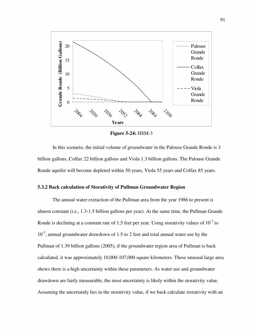
91

0

5

10

15

20

20042020

20362052

20682084

2100

Years

Gra

nd

e R

on

de

(B

illi

on

Ga

llo

ns)

PalouseGrande

Ronde

Colfax

Grande

Ronde

Viola

Grande

Ronde

Figure 5-24: HSM-3

In this scenario, the initial volume of groundwater in the Palouse Grande Ronde is 3

billion gallons, Colfax 22 billion gallons and Viola 1.3 billion gallons. The Palouse Grande

Ronde aquifer will become depleted within 50 years, Viola 55 years and Colfax 85 years.

5.3.2 Back calculation of Storativity of Pullman Groundwater Region

The annual water extraction of the Pullman area from the year 1986 to present is

almost constant (i.e., 1.3-1.5 billion gallons per year). At the same time, the Pullman Grande

Ronde is declining at a constant rate of 1.5 feet per year. Using storativity values of 10-3 to

10-5, annual groundwater drawdown of 1.5 to 2 feet and total annual water use by the

Pullman of 1.39 billion gallons (2005), if the groundwater region area of Pullman is back

calculated, it was approximately 10,000-107,000 square kilometers. These unusual large area

shows there is a high uncertainty within these parameters. As water use and groundwater

drawdown are fairly measurable, the most uncertainty is likely within the storativity value.

Assuming the uncertainly lies in the storativity value, if we back calculate storativity with an

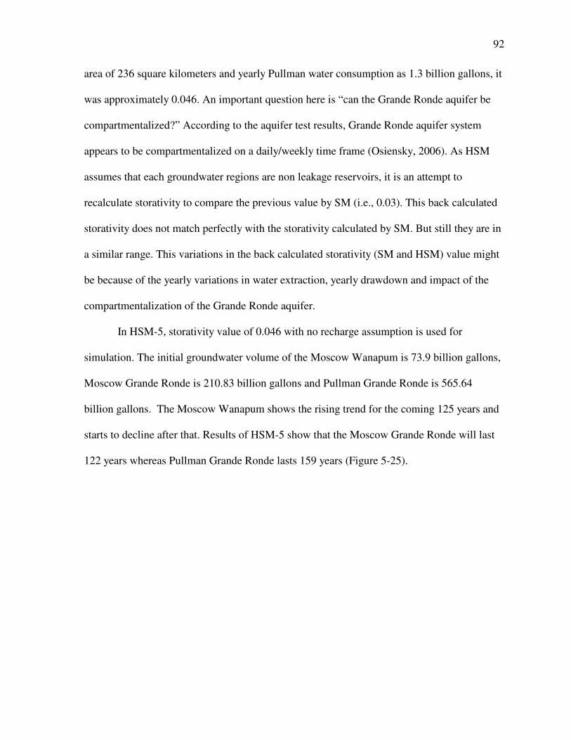
92

area of 236 square kilometers and yearly Pullman water consumption as 1.3 billion gallons, it

was approximately 0.046. An important question here is “can the Grande Ronde aquifer be

compartmentalized?” According to the aquifer test results, Grande Ronde aquifer system

appears to be compartmentalized on a daily/weekly time frame (Osiensky, 2006). As HSM

assumes that each groundwater regions are non leakage reservoirs, it is an attempt to

recalculate storativity to compare the previous value by SM (i.e., 0.03). This back calculated

storativity does not match perfectly with the storativity calculated by SM. But still they are in

a similar range. This variations in the back calculated storativity (SM and HSM) value might

be because of the yearly variations in water extraction, yearly drawdown and impact of the

compartmentalization of the Grande Ronde aquifer.

In HSM-5, storativity value of 0.046 with no recharge assumption is used for

simulation. The initial groundwater volume of the Moscow Wanapum is 73.9 billion gallons,

Moscow Grande Ronde is 210.83 billion gallons and Pullman Grande Ronde is 565.64

billion gallons. The Moscow Wanapum shows the rising trend for the coming 125 years and

starts to decline after that. Results of HSM-5 show that the Moscow Grande Ronde will last

122 years whereas Pullman Grande Ronde lasts 159 years (Figure 5-25).

93

0

100

200

300

400

500

600

20042040

20762112

21482184

Years

Gra

nd

e R

on

de

(Billio

n

Ga

llo

ns)

0

50

100

150

200

250

Mo

scow

Wa

na

pu

m (

Bil

lio

n

Ga

llon

s)

Moscow

Grande

Ronde

Pullman

GrandeRonde

Moscow

Wanapum

Figure 5-25: HSM-5

This condition satisfies the present water level trend of Moscow and Pullman Grande

Ronde but the Wanapum is not realistic.

5.4 HSM for Water Resource Management with Current Infrastructures

HSM-4 is used to evaluate the Moscow groundwater situation assuming the Moscow

Wanapum will fulfill the entire Moscow water demand when Moscow Grande Ronde

becomes minimum value (Section 4.5.1, Equations 4-9, 4-10 and 4-11). In this applied

condition, the Moscow Grande Ronde will last for 5 years and the water demand is fulfilled

by the Moscow Wanapum. But Moscow Wanapum is able to fulfill the water demand only

for about 64 years. After 64 years, the Moscow water demand is greater than the Moscow

groundwater and recharge (Figure 5-26). There are no options for the Pullman Grande

Ronde.

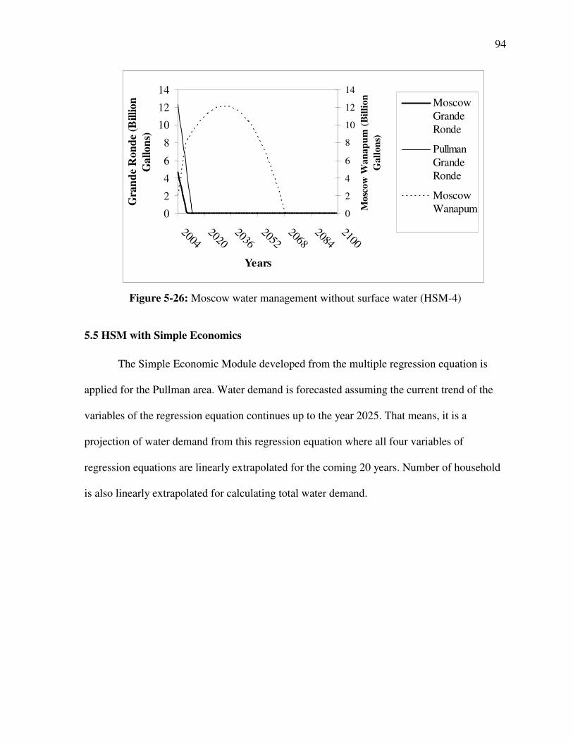
94

0

2

4

6

8

10

12

14

20042020

20362052

20682084

2100

Years

Gra

nd

e R

on

de

(Billio

n

Ga

llo

ns)

0

2

4

6

8

10

12

14

Mo

scow

Wa

na

pu

m (

Bil

lio

n

Ga

llon

s)

Moscow

Grande

Ronde

Pullman

GrandeRonde

Moscow

Wanapum

Figure 5-26: Moscow water management without surface water (HSM-4)

5.5 HSM with Simple Economics

The Simple Economic Module developed from the multiple regression equation is

applied for the Pullman area. Water demand is forecasted assuming the current trend of the

variables of the regression equation continues up to the year 2025. That means, it is a

projection of water demand from this regression equation where all four variables of

regression equations are linearly extrapolated for the coming 20 years. Number of household

is also linearly extrapolated for calculating total water demand.

95

Figure 5-27: Linear Extrapolation of Independent variables for Regression Equation

Figure 5-27 shows the linear extrapolation of variables up to the year 2025 (except

precipitation with constant annual areal mean precipitation). The constant increase in water

price in the Simple Economic module predicts decrease in water demand. It is because of the

complex interaction among these variables.

00.5

11.5

22.5

2000 2010 2020 2030

Years

Marg

ina

l P

rice

($/1

00ft

3)

010

2030

4050

2000 2010 2020 2030

Years

Fix

ed P

rice

($ f

or

1"

met

er)

0

10,000

20,000

30,000

40,000

2000 2010 2020 2030

Years

Med

ian

Hou

seh

old

Inco

me

($)

2.122.142.162.182.2

2.222.24

2000 2010 2020 2030

Years

Aver

age

Hou

seh

old

Siz

e

0

10

20

30

2000 2010 2020 2030

Years

Mea

n A

real

Pre

cip

itati

on

(in

ches

)

9,000

9,500

10,000

10,500

11,000

2000 2010 2020 2030

Years

No. of

Hou

seh

old

s

96

0

0.1

0.2

0.3

0.4

0.5

0.6

0.7

0.8

2004 2009 2014 2019 2024

Years

Wate

r D

eman

d (

Bil

lio

n G

all

on

s)

Figure 5-28: Water Demand Projection by Economic Module

This projection of water demand refers (Figure 5-28) to the regression Equation 4-7.

This equation was developed from the total water consumption of residential sector. Because

of lack of exact number of service connections in different user’s class, the water demand

from Economic Module did not match perfectly to the Water Demand Module. Water

demand projected from Demand Module shows the constant increase of water demand of

Pullman but conversely the Economic Module predicts decrease. Figure 5-28 shows the

water demand projection from the Economic Module (i.e., regression equation). The

Economic Module projects the water demand of City of Pullman about 0.75 billion gallons in

the year 2005. But the projected water demand in the coming 20 years decreases rapidly in

the applied condition. Obliviously, decrease in water demand will decrease in per capita per

day water use. This per capita per day water use by economic module can be used by

population model but because of the lack of integrated study in entire Palouse Region, this

per capita water use is not used in this study.

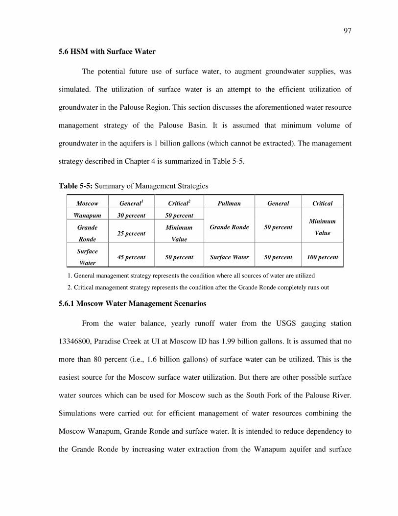
97

5.6 HSM with Surface Water

The potential future use of surface water, to augment groundwater supplies, was

simulated. The utilization of surface water is an attempt to the efficient utilization of

groundwater in the Palouse Region. This section discusses the aforementioned water resource

management strategy of the Palouse Basin. It is assumed that minimum volume of

groundwater in the aquifers is 1 billion gallons (which cannot be extracted). The management

strategy described in Chapter 4 is summarized in Table 5-5.

Table 5-5: Summary of Management Strategies

Moscow General1 Critical

2 Pullman General Critical

Wanapum 30 percent 50 percent

Grande

Ronde 25 percent

Minimum

Value

Grande Ronde 50 percent Minimum

Value

Surface

Water 45 percent 50 percent Surface Water 50 percent 100 percent

1. General management strategy represents the condition where all sources of water are utilized

2. Critical management strategy represents the condition after the Grande Ronde completely runs out

5.6.1 Moscow Water Management Scenarios

From the water balance, yearly runoff water from the USGS gauging station

13346800, Paradise Creek at UI at Moscow ID has 1.99 billion gallons. It is assumed that no

more than 80 percent (i.e., 1.6 billion gallons) of surface water can be utilized. This is the

easiest source for the Moscow surface water utilization. But there are other possible surface

water sources which can be used for Moscow such as the South Fork of the Palouse River.

Simulations were carried out for efficient management of water resources combining the

Moscow Wanapum, Grande Ronde and surface water. It is intended to reduce dependency to

the Grande Ronde by increasing water extraction from the Wanapum aquifer and surface

98

water. The management strategy of the Moscow area is to reduce the dependency on the

Grande Ronde by 45 percent by utilizing surface water. In this situation, about 30 percent

water from the Wanapum, 25 percent from the Grande Ronde and rest 45 percent from the

surface water is utilized (Table 5-5). Figure 5-29 shows the water extraction pattern of

Moscow as in the HSM-3. In HSM-3, without recharge to the Grande Ronde and storativity

of 0.0001 is used.

0

0.2

0.4

0.6

0.8

1

1.2

1.4

1.6

1.8

20042020

20362052

20682084

2100

Years

Wa

ter

Ex

tra

ctio

n (

Bil

lio

n G

all

on

s)

Moscow

Grande

Ronde

Extraction

Moscow

Surface

Water

Extraction

Moscow

Wanapum

Extraction

Figure 5-29: Water Extraction Pattern of Moscow (HSM-3)

Without recharge to the Grande Ronde and with low storativity value, combined with

the surface water, the Moscow Grande Ronde faces deficiency almost instantly. Figure 5-29

shows the Water extraction pattern of the Moscow Grande Ronde, Wanapum and the surface

water. In this management strategy, the water demand is fulfilled by Moscow Wanapum and

surface water. Figure 5-30 shows the groundwater level pattern of the Moscow Wanapum

and Grande Ronde aquifer as in the HSM-3. In the applied infrastructure condition, the initial

groundwater volume in the Moscow Grande Ronde is less than a billion gallon and remains

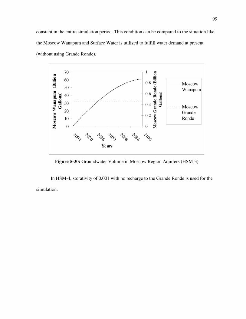
99

constant in the entire simulation period. This condition can be compared to the situation like

the Moscow Wanapum and Surface Water is utilized to fulfill water demand at present

(without using Grande Ronde).

0

10

20

30

40

50

60

70

20042020

20362052

20682084

2100

Years

Mo

sco

w W

an

ap

um

(B

illi

on

Ga

llo

ns)

0

0.2

0.4

0.6

0.8

1

Mo

sco

w G

ran

de

Ro

nd

e (B

illi

on

Gall

on

s)

MoscowWanapum

MoscowGrande

Ronde

Figure 5-30: Groundwater Volume in Moscow Region Aquifers (HSM-3)

In HSM-4, storativity of 0.001 with no recharge to the Grande Ronde is used for the

simulation.

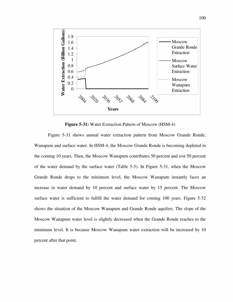
100

0

0.2

0.4

0.6

0.8

1

1.2

1.4

1.6

1.8

20042020

20362052

20682084

2100

Years

Wa

ter

Ex

tra

ctio

n (

Billio

n G

allo

ns)

Moscow

Grande Ronde

Extraction

Moscow

Surface WaterExtraction

Moscow

Wanapum

Extraction

Figure 5-31: Water Extraction Pattern of Moscow (HSM-4)

Figure 5-31 shows annual water extraction pattern from Moscow Grande Ronde,

Wanapum and surface water. In HSM-4, the Moscow Grande Ronde is becoming depleted in

the coming 10 years. Then, the Moscow Wanapum contributes 50 percent and rest 50 percent

of the water demand by the surface water (Table 5-5). In Figure 5-31, when the Moscow

Grande Ronde drops to the minimum level, the Moscow Wanapum instantly faces an

increase in water demand by 10 percent and surface water by 15 percent. The Moscow

surface water is sufficient to fulfill the water demand for coming 100 years. Figure 5-32

shows the situation of the Moscow Wanapum and Grande Ronde aquifers. The slope of the

Moscow Wanapum water level is slightly decreased when the Grande Ronde reaches to the

minimum level. It is because Moscow Wanapum water extraction will be increased by 10

percent after that point.

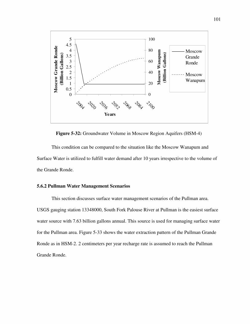
101

0

0.5

1

1.5

2

2.5

3

3.5

4

4.5

5

20042020

20362052

20682084

2100

Years

Mo

sco

w G

ran

de

Ro

nd

e

(Bil

lio

n G

all

on

s)

0

20

40

60

80

100

Mo

sco

w W

an

ap

um

(Bil

lio

n G

all

on

s)

MoscowGrande

Ronde

MoscowWanapum

Figure 5-32: Groundwater Volume in Moscow Region Aquifers (HSM-4)

This condition can be compared to the situation like the Moscow Wanapum and

Surface Water is utilized to fulfill water demand after 10 years irrespective to the volume of

the Grande Ronde.

5.6.2 Pullman Water Management Scenarios

This section discusses surface water management scenarios of the Pullman area.

USGS gauging station 13348000, South Fork Palouse River at Pullman is the easiest surface

water source with 7.63 billion gallons annual. This source is used for managing surface water

for the Pullman area. Figure 5-33 shows the water extraction pattern of the Pullman Grande

Ronde as in HSM-2. 2 centimeters per year recharge rate is assumed to reach the Pullman

Grande Ronde.

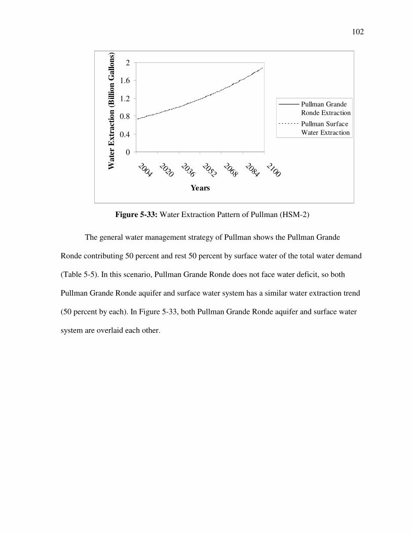
102

0

0.4

0.8

1.2

1.6

2

20042020

20362052

20682084

2100

Years

Wa

ter

Ex

tra

ctio

n (

Billio

n G

allo

ns)

Pullman Grande

Ronde Extraction

Pullman Surface

Water Extraction

Figure 5-33: Water Extraction Pattern of Pullman (HSM-2)

The general water management strategy of Pullman shows the Pullman Grande

Ronde contributing 50 percent and rest 50 percent by surface water of the total water demand

(Table 5-5). In this scenario, Pullman Grande Ronde does not face water deficit, so both

Pullman Grande Ronde aquifer and surface water system has a similar water extraction trend

(50 percent by each). In Figure 5-33, both Pullman Grande Ronde aquifer and surface water

system are overlaid each other.

103

0

5

10

15

20

25

30

35

20042020

20362052

20682084

2100

Years

Pu

llm

an

Gra

nd

e R

on

de

(Billio

n G

allo

ns)

Figure 5-34: Groundwater Volume in Pullman Region Aquifers (HSM-2)

Figure 5-34 shows the groundwater level pattern of the Pullman Grande Ronde

aquifer when recharge rate is 2 centimeters per year (Scenario 2).The groundwater volume

increases to 32 billion gallons in the coming 60 years and continues to decrease after that. It

reaches 23 billion at the end of the 100 years.

In HSM-4, the storativity value of 0.001 was used with no recharge to the Grande

Ronde aquifer (Table 5-4).

104

0

1

2

3

4

20052021

20372053

20692085

Years

Wa

ter

Ex

tra

ctio

n (

Billio

n G

allo

ns)

Pullman Grande

Ronde Extraction

Pullman Surface

Water Extraction

Figure 5-35: Water Extraction Pattern of Pullman (HSM-4)

Figure 5-35 shows the water extraction pattern of the Pullman area as in HSM-4. In

the applied conditions, the Pullman Grande Ronde will become depleted within 15 years

(Figure 5-36) and the deficit in the water demand is fulfilled by surface water systems. After

this point, the entire Pullman water demand is fulfilled by the surface water. Figure 5-35

shows jump in surface water extraction to balance water demand when the Pullman Grande

Ronde reaches to the minimum level. This condition can be compared to the situation like the

Pullman Surface water is utilized to fulfill water demand after 15 years irrespective to the

volume of the Grande Ronde.

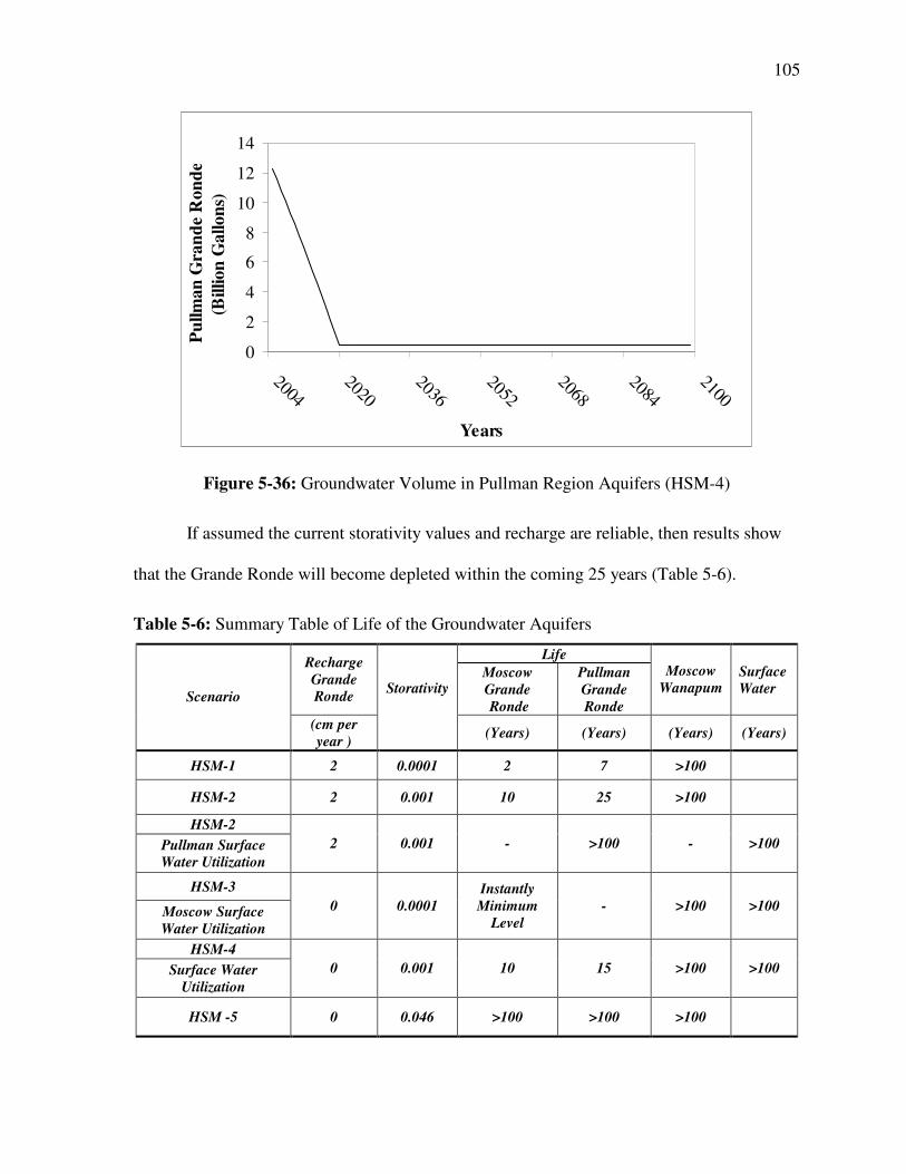
105

0

2

4

6

8

10

12

14

20042020

20362052

20682084

2100

Years

Pu

llm

an

Gra

nd

e R

on

de

(Billio

n G

allo

ns)

Figure 5-36: Groundwater Volume in Pullman Region Aquifers (HSM-4)

If assumed the current storativity values and recharge are reliable, then results show

that the Grande Ronde will become depleted within the coming 25 years (Table 5-6).

Table 5-6: Summary Table of Life of the Groundwater Aquifers

Life Recharge

Grande

Ronde

Moscow

Grande

Ronde

Pullman

Grande

Ronde

Moscow

Wanapum

Surface

Water

Scenario

(cm per

year )

Storativity

(Years) (Years) (Years) (Years)

HSM-1 2 0.0001 2 7 >100

HSM-2 2 0.001 10 25 >100

HSM-2

Pullman Surface

Water Utilization

2 0.001 - >100 - >100

HSM-3

Moscow Surface

Water Utilization

0 0.0001

Instantly

Minimum

Level

- >100 >100

HSM-4

Surface Water

Utilization

0 0.001 10 15 >100 >100

HSM -5 0 0.046 >100 >100 >100

106

In the above discussed water management strategies, more than 50 percent water is

intended to be utilized from the surface water. The yearly runoff in the USGS gauging station

13348000 at South Fork Palouse River at Pullman is 7.63 billion gallons. The projected water

demand of the Pullman area after 100 years is about 4.2 billion gallons. In terms of quantity,

utilizing this source alone is still sufficient to fulfill the water demand of the Pullman area.

But the situation of Moscow area is slightly different. The Paradise Creek at UI at Moscow

ID is not sufficient to fulfill the Moscow demand and some other source should be combined

with this source.

5.7 Surface Water

The management strategies discussed above in the surface water utilization section

provide an overall picture of surface water utilization. Feasibility study of the particular

streams is a preliminary step for utilizing surface water. Figure 5-37 shows South Fork

Watershed with different sub-watersheds delineated from four major sources of surface water

(i.e., South Fork River at Palouse, Paradise Creek, Missouri Flat Creek and Fourmile Creek).

A brief discussion will be carried out of the Paradise Creek and South Fork Palouse River at

Pullman in this section. The available surface water flow of the Paradise Creek and South

Fork Palouse River is to be determined for sizing reservoir. The origin of both rivers is the

Moscow Mountain. Paradise Creek meets the South Fork Palouse River in Pullman.

107

Figure 5-37: South Fork Palouse River Sub-Basins

(South Fork Palouse River Watershed Characterization and Implementation Plan, 2002)

The key question here is how much water can be withdrawn from these sources per

day. Flow requirements should be calculated to find out how much minimum water is

required for the source. Mass balance should be carried out for calculating consistent water

supply of a reservoir at certain capacity. Table 5-7 shows the summary of two sources of

surface water in local scale (USGS gauging stations). As in the management strategy, 50

percent of the total demand is intended to fulfill by Paradise Creek and 100 percent by South

Fork Palouse River at Pullman. The maximum reservoir supply in the Table 5-7 is a daily

water demand at the year 2100. The size and location of reservoir should be determined in

the feasibility study and detailed design phase. Table 5-7 also shows the mean, minimum and

maximum daily discharge of these sources of surface water. Both Moscow and Pullman can

be benefited by the South Fork Palouse River; the water allocation issue of this river is

important.

108

Table 5-7: Summary of Paradise Creek and South Fork Palouse at Pullman

Parameters

Moscow

(Paradise

Creek)

Pullman

(SF Palouse)

Source

Area 45.65 284.35 Watershed map

Daily Discharge

Period of Availability

10/01/1978-

09/30/2006

02/01/1934-

09/30/2006 USGS

Maximum Water Use

60 percent 100 percent Management Strategy

Maximum Water Demand

Fulfilled by Reservoir

(Billion Gallons per year)

1.9 3.79 Demand Forecast

(Year 2100)

Maximum Reservoir Supply

(Million gallons per day) 5.3 10.38

Demand Forecast

(Year 2100)

Mean Annual Flow

(cubic feet per sec) 9.5 39.2 Golder Associates, 2004

Maximum Annual Flow

(cubic feet per sec) 11.7 111.3 Golder Associates, 2004

Minimum Annual Flow (cubic

feet per sec) 1.5 7.7 Golder Associates, 2004

Table 5-8 shows the surface water result conducted by WRIA -34. Results of summer

period (June to October) of the year 2025 are shown.

Table 5-8: Estimated Surface Water Availability (Stasney, 2006)

Community (Water Source) Paradise Creek at

University of Idaho

South Fork

Palouse River at

Pullman

USGS 13346800 1334800

2025 Summer (June – October)

Demand

Acre Foot 3582 4516

Billion Gallons 1.17 1.47

Surface Water Available for Diversion Nov-May Nov-May

Percent Summer Demand available 10-20 percent 50-100 percent

5.8 Sustainability Index (SI)

SI is calculated from the ratio of annual water demand (extraction) to annual

recharge. The SI of the Grande Ronde with respect to the total demand is calculated as in

applied condition in HSM-6. Equation 4-18 is used to calculate SI of the Grande Ronde and

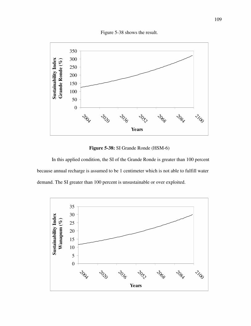
109

Figure 5-38 shows the result.

0

50

100

150

200

250

300

350

20042020

20362052

20682084

2100

Years

Su

sta

ina

bilit

y I

nd

ex

Gra

nd

e R

on

de

(%)

Figure 5-38: SI Grande Ronde (HSM-6)

In this applied condition, the SI of the Grande Ronde is greater than 100 percent

because annual recharge is assumed to be 1 centimeter which is not able to fulfill water

demand. The SI greater than 100 percent is unsustainable or over exploited.

0

5

10

15

20

25

30

35

20042020

20362052

20682084

2100

Years

Su

sta

ina

bilit

y I

nd

ex

Wa

na

pu

m (

%)

110

Figure 5-39: SI Wanapum (SM-4)

SI of the Wanapum is evaluated as according to the SM-4 and calculated as according

to Equation 4-17. Results show the SI of the Wanapum starts at 12 percent and reaches at 30

percent in the coming 100 years (Figure 5-39). The results show it is sustainable.

The SI of the Wanapum basically represents the sustainability of groundwater

systems of the Palouse Basin. It is the comparison of the total recharge of the Palouse Basin

to the total demand. But still the controversies remain here because even if the recharge to

the Wanapum is assumed to be correct, there is no evidence that this water is stored for the

future use, given that the present water level is almost constant and there is no gain in water

level.

5.9 Summary

The designated area of the groundwater region that gets recharged is about 769 square

kilometers compared to 2,044 square kilometers surface area of watershed. The recharge to

the Wanapum is 4.7 centimeters and approximately 13 billion gallons water enters in the

designated groundwater regions annually. The initial volume of groundwater in the

Wanapum ranges from 0.06 to 40.16 billion gallons whereas the Grande Ronde ranges from

0.95 to 43 billion gallons with the storativity values of 10-5 to 10-3. Negligible amount (less

than 4-6 millimeters per year) of recharged water should enter to the Wanapum aquifer for

fairly stable water level. SM projects that the volume of water in the Wanapum rises up to 2

trillion gallons whereas HSM projects 150 billion gallons in the coming 100 years. Results

show that the Grande Ronde depletes at an alarming rate in a lower storativity value. The

back calculated storativity value ranges from 0.03 to 0.046 which projects the present water

depletion trend in the Grande Ronde. The Grande Ronde groundwater will last for maximum

111

80 years (both by SM and HSM) in the present infrastructures in an optimistic condition. The

rising trend of the Wanapum and declining trend of the Grande Ronde both did not match to

the present water level trend with the current storativity values.

The marginal price of water is increased from $ 0.32 to $ 1.5 for 100 cubic feet from

the 1970 to date. The price elasticity of demand of the marginal price ranges from +1.6 to

+2.95. The price elasticity of demand showed a little relation between the marginal water

pricing and demand.

Even if 50 percent of water demand is intended to fulfill by surface water from the

present date, because of the small initial groundwater volume in the Grande Ronde, the

Grande Ronde aquifer will deplete within couple of years. So, the sustainability of the

Grande Ronde is one of the challenges to water scientists.

112

CHAPTER VI

CONCLUSIONS

6.0 Overview

In this chapter, the conclusions of overall study are presented. The use of the System

Dynamics Approach for water resources management is discussed in the first section. Results

of the SM and HSM for understanding the Wanapum and Grande Ronde are discussed in the

second and third sections. The usefulness of the developed regression equation for computing

the price elasticity of water demand and for the modeling is discussed. Discussion will be

carried out regarding problems in defining the sustainability of groundwater of this basin.

Also the quality of data and possible impacts in the modeling is described. In the final

section, some future recommendations and limitations about the study are presented.

6.1 System Dynamics Approach

The use of a System Dynamics Approach for managing water resources has wide

applications. It has opened a number of opportunities for modeling water resources in a small

watershed level to the global scale. The beauty of these types of modeling approach is to

develop models by close supervision and suggestions of experts in specific fields

incorporating the general public. Another equally important aspect of System Dynamics

Approach is to model technical and social aspect together with very little knowledge of

programming. The hydrological model (technical) with simple population (social) and

economic module is linked in this process. The important aspect of this research is to develop

system dynamics model of the Palouse Basin Watershed and draw some conclusions from

these models.

113

6.2 SM and HSM

To study the current groundwater pattern and project future groundwater scenarios,

SM and HSM model were developed. The basic philosophy of the SM and HSM is similar.

Both models do not account for lateral flows. The external boundaries of the groundwater

regions are fixed. In SM, the regions share the groundwater each other but in HSM, each

region rely on its corresponding groundwater. In HSM, the groundwater in the Grande Ronde

in each region is comparatively small compared to the demand. So, the life of the Moscow

and Pullman aquifer is smaller in HSM compared to SM.

6.3 Wanapum and Grande Ronde

The current storativity, potential groundwater drawdown and surface area of

groundwater showed only a small amount of groundwater stored in both the Wanapum and

Grande Ronde aquifer. Results show that the water level of the Wanapum will rise rapidly

according to the computed water balance in the coming years. There are three possible

reasons of increasing water level trend in the Wanapum. The first possibility is the areal

mean recharge rate to the Wanapum is lower than calculated from the water balance. The

second possibility is the recharged water of the entire Wanapum can not be lumped or

Wanapum groundwater region is compartmentalized. Results show that the adjusted annual

volumetric recharge rate to the Wanapum is less than a billion gallons which is only a tiny

part of the total recharge (13 billion gallons) computed by the overall water balance.

The present water extraction from the Moscow Wanapum is about 0.26 billion

gallons in the year 2005. If the Wanapum is assumed as a non-leakage reservoir, the same

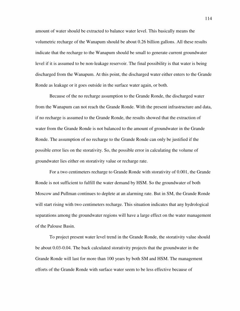
114

amount of water should be extracted to balance water level. This basically means the

volumetric recharge of the Wanapum should be about 0.26 billion gallons. All these results

indicate that the recharge to the Wanapum should be small to generate current groundwater

level if it is assumed to be non-leakage reservoir. The final possibility is that water is being

discharged from the Wanapum. At this point, the discharged water either enters to the Grande

Ronde as leakage or it goes outside in the surface water again, or both.

Because of the no recharge assumption to the Grande Ronde, the discharged water

from the Wanapum can not reach the Grande Ronde. With the present infrastructure and data,

if no recharge is assumed to the Grande Ronde, the results showed that the extraction of

water from the Grande Ronde is not balanced to the amount of groundwater in the Grande

Ronde. The assumption of no recharge to the Grande Ronde can only be justified if the

possible error lies on the storativity. So, the possible error in calculating the volume of

groundwater lies either on storativity value or recharge rate.

For a two centimeters recharge to Grande Ronde with storativity of 0.001, the Grande

Ronde is not sufficient to fulfill the water demand by HSM. So the groundwater of both

Moscow and Pullman continues to deplete at an alarming rate. But in SM, the Grande Ronde

will start rising with two centimeters recharge. This situation indicates that any hydrological

separations among the groundwater regions will have a large effect on the water management

of the Palouse Basin.

To project present water level trend in the Grande Ronde, the storativity value should

be about 0.03-0.04. The back calculated storativity projects that the groundwater in the

Grande Ronde will last for more than 100 years by both SM and HSM. The management

efforts of the Grande Ronde with surface water seem to be less effective because of

115

extremely low quantity in groundwater. More surface water has to be used to fulfill the

deficit of groundwater in the future.

6.4 Watershed Economics

There are different reasons for positive marginal price elasticity. The first possibility

is that people might not be aware of the water demand and pricing structures. It means the

price is not influencing directly the water demand at present. Secondly, the quality of data is

affecting the results. The time series data without exact service connections and monthly

data, questions can be aroused on the reliability of analysis. Thirdly, a city like Pullman

where more than half population is students, the housing and water use pattern is complex.

Also the increasing block rate structures for different user classes and time period add

complexities to the analysis. Results show the coefficient of determination is weak in all

cases.

It should be clearly understood that the water pricing structures of the City of Pullman

is complex. This attempt to calculate price elasticity is widely limited by data quality, time

frame and main objectives of the study. In particular, analysis provided here has not

accounted for changes in the dollar amounts used based on constant dollars. As the economic

study is only one of the components of this study, more in-depth study in this topic is

necessary. The main interest here is to use these results in the economic module developed in

System Dynamics Approach.

6.5 Sustainability of Aquifers

Results of HSM show the SI of the Grande Ronde is greater than 100 percent even

with the recharge assumption. It basically means the small recharge rate with the current

116

storativity values is not able to fulfill the water demand. It is because of the low initial

volume of the Grande Ronde. These conditions indicating that the Grande Ronde aquifer is at

high risk and it is being exploited in an unsustainable way.

Because of non-leakage assumptions from the Wanapum, results show the water level

of the Wanapum is in the increasing trend. But, the sustainability issue of the Wanapum

aquifer is equally important because of the past fluctuating water level trend. The water level

depletion and recovery (1940s to 1960s) of the Wanapum indicates that the Wanapum is not

out of risk. More extraction from the Wanapum may cause water level depletion but within

the limit of current assumptions, the Wanapum seems to be sustainable.

6.6 Calibration and Validations

The attempt to project the present water level depletion trend of the Wanapum and

Grande Ronde arises many questions. Results show that either recharge rate to the Wanapum

should be small than the computed water balance values or recharge water of the Wanapum

should reach to the Grande Ronde (if assumed less influence of the discharged water from

the Wanapum). This justifies the inter-relationship between the Wanapum and Grande

Ronde. Assuming recharge from the water balance is satisfactory, to project the present water

level trend, there should be some recharge to the Grande Ronde. Back calculated storativity

with the present infrastructure and water use pattern shows a realistic trend of water depletion

pattern. These are the certain attempts to look in the topic of calibrating and validating the

model. Sensitivity analysis from SM shows even if the Wanapum and Grande Ronde are

getting larger recharge rates, because of the small storativity values, the life of these aquifers

are shorter compared to other scenarios. The interesting fact here is the lives of these aquifers

are more dominated by the storativity values (i.e., initial water storage in the aquifers).

117

Sensitivity analyses projects the present water level trend with about 100 years life difference

depending on the applied conditions. So, these issues make water resource management of

the Palouse Basin more complicated.

6.7 Data and Results Quality

The reliability of any model depends on the availability of data, appropriateness of

assumptions and structural formation of the model. Significant amounts of data were

collected and generated for this study. This section briefly addresses data uncertainty.

Uncertainty in the water balance components, particularly evapotranspiration which is

expected to be more uncertain than precipitation and runoff, leads to uncertainties in

recharge.

The reliability of the geologic data directly affects the amount of water stored in

aquifers. Because of the complexities of the geologic formation and lack of integrated study,

the availability of geologic data in the Palouse Basin is limited. The storativity values affect

tremendously the initial groundwater volume. The accuracy of these results basically depends

on the components of water balance and initial storage of groundwater in the aquifers. In

terms of water balance, evapotranspiration rate is the most susceptible component as it is

difficult to calculate accurately. Because evapotranspiration is large compared to recharge,

relatively small errors in estimating evapotranspiration can lead to relatively large errors in

recharge. The calculation of volume of groundwater in the aquifers fluctuated widely by the

uncertainties in parameters which affects the overall results. The back area calculation

further justified that the lower storativity value plays a vital role in calculating the small

amount of groundwater in the aquifers. Because of the uncertainties in groundwater volume,

some of the other important parameters like population growth are not altered in this

118

modeling process.

The uncertainty in data of a simple economic module is another challenge. Because of

a lack of exact data, linear interpolation was used to generate monthly data. Also the number

of exact service connections which use the total amount of water could not be found within

the scope of this study.

6.8 Summary

The overarching goal of this study was to model, using implying assumptions and

available data, how water resources of the Palouse Region might behave and be managed.

The possible management strategy in this context is to decrease the dependency on the

groundwater by switching to surface water. If the current storativity and recharge values are

considered reliable; the only option for managing water resources is to decrease dependence

on the Grande Ronde. Further, these results are also indicating that within the present

infrastructures, if no recharge to the lower aquifers is assumed, these aquifers are not able to

fulfill the water demand of the Palouse Basin in a sustainable way. The availability of

appropriate data is equally important. The accurateness of these results depends on the

adopted models and the quality of data.

6.9 Recommendations

The variability in the major components of groundwater makes difficult to draw any

conclusions about the water resources of the Palouse Basin. Even if, after considering many

technical details of groundwater systems, many questions are yet to be answered. In future,

greater confidence in these parameters, should allow us to narrow down the variability in the

results. Definitely, the future research should concentrate on lessening this variability.

119

The primary step to define the groundwater sustainability of this basin is to finalize the initial

groundwater volume of the aquifers. The initial groundwater volume of these aquifers is

governed by the storativity. The wide variability in the storativity value makes it difficult to

quantify groundwater and consequently the life of these aquifers. So storativity is the most

important parameters which should be the main focus of future research. The recharge rate to

the Wanapum is an equally important parameter. Even if, the recharge of the water balance

showed that the water level of the Wanapum aquifer is rising but in fact it is not the case in

reality. The recharge rate is not a single factor that makes the Wanapum level rise. This

phenomenon is also affected by the water that is being discharged from the Wanapum (not

accounted in this whole process) and probable recharge to the Grande Ronde. So, the

recharged water to the Wanapum can be divided into three components. The first and major

portion of recharge will stay in the Wanapum aquifer, the second will be discharged from

streams and springs and finally some portion will reach the Grande Ronde as recharge.

It is difficult to account how much water is discharged from numerous streams and

springs and how much enters in the Grande Ronde. Researches have proved that water being

discharged from Wanapum. The SM and HSM models used by this study did not incorporate

discharged water from the Wanapum. Figure 6-1 shows the future model that includes

discharged water from the Wanapum.

120

Figure 6-1: Future Schematic of SM of the Palouse Basin

The recharge mechanism to the Grande Ronde aquifer is another challenge in this

process. It is the fraction of water that is recharged from the Wanapum. These mechanisms

should be understood clearly for managing groundwater resources of the Palouse Basin. In

the future, the water balance will be more complicated with three components (i.e., the

recharge to the Wanapum, discharge from the Wanapum and recharge to the Grande Ronde).

As surface water is assumed to replace groundwater in the future, the focus on the

surface water needs to be increased. The present model structure assumes that eighty percent

Recharge by

Water Balance

Upper Aquifer

Wanapum

Lower Aquifer

Grande Ronde

Surface Water

Watershed

Leakage by

Assumption

Surface Water

(Springs, Streams)

Discharge

121

of the runoff water can be potentially utilized. But the detailed surface water assessment

should be carried out. It should be understood that the above discussed water management

strategies are only some of the probable options. After finalizing the study of the surface

water sources, combined utilization of surface water and groundwater for efficient water

resources management should be finalized. Consequently, the location and size of the

reservoir should be accounted in the future study.

The water demand economics is another sector where additional research can be

carried out. This study is an attempt to understand price elasticity of demand. Because of the

limited data, only the Pullman area is included in this research but still results are not

satisfactory. In future, the entire basin situation should be studied. At the same time, the

verification of data and reliability of analysis of the regression equation including price

inflation should be conducted in future. It is recommended that further research consider to

carry in-depth study of this subject matter in the future.

For sustainable water resources, all the components of water resources are equally

important. This research has focused on the groundwater and surface water hydrology with

population and some economic aspects. Future research should incorporate other components

like environmental and legal issues as of the water resources. The important question

regarding the sustainability of the Grande Ronde aquifer can not be answered unless the

recharge to the Grande Ronde is estimated reliably. If the Grande Ronde is assumed to have

no recharge, it is difficult to assess the sustainability of this aquifer.

Finally, there are numerous tools in the STELLA software for effective modeling

which can be further utilized in future research. The present model can be further modified

and shortened by adding more codes and boundary conditions.

122

The Palouse Region is solely dependent on the Grande Ronde aquifer for drinking

water and still this study did not address all the questions. This research can act as a base for

further understanding of these aquifers and utilizing a System Dynamics Approach to

manage water resources in the Palouse Region. More work should be done to utilize these

results in the planning process. It is an attempt to understand the future water resource

scenario from the past and present trend. Here more focus is to make a usable and workable

model. Ford (1999) in his book “Modeling the Environment” has included some concluding

remarks about the system dynamics where he emphasized the usefulness of the model rather

than validation.

6.10 Limitations

While every effort has been taken to ensure the accuracy of information presented in

this thesis, this should not be considered to be a “peer-reviewed” document. The simulation

scenarios are hypothetical. Therefore, the data, information, results, and conclusions should

not be used in legal matters including, but not limited to, water rights determinations and

transfers, without further review and analysis.

123

REFERENCES

Ahmad, S., and Simonovic, S.P., 2004. Spatial system dynamics: new approach for simulation of water resources systems. Journal of Computing in Civil Engineering, Vol. 18, No. 4©ASCE, ISSN 0887-3801/2004/4-331–340.

Anderson, M.T., and Woosley, L.H., Jr, 2002. Science to support the management of western

water. The Geological Societies of America Conference, Denver, CO. ASCE, 1998. Sustainability criteria for water resource systems. Task Committee on

Sustainability Criteria, Water Resource Planning and Management Division. ASCE and Working Group, UNESCO/IHP IV Project M-4.3.

Badon, N. M. and Osiensky, J. L., 2007. Implementation of a groundwater monitoring

program and aquifer testing in the Wanapum Aquifer System, Latah County, Idaho County, Idaho. Master degree thesis, Department of Geological Sciences, University of Idaho.

Bloomsburg, G.L., 1959. A water balance study of two small watersheds, University o Idaho,

Moscow, 66 pp. Bush, J. and Hinds, J., 2006. Geologic overview of the Palouse Basin. Palouse Basin Water

Summit, Moscow ID. City of Moscow, 1999. Comprehensive Plan. Cook, Z., Urban, S., Maupin, M., Pratt, R., and Church, J., 2001. Domestic, commercial,

municipal and industrial water demand assessment and forecast in Ada and Canyon Counties, Idaho.

Crosby III, J.W., and Chatters, R.M., 1965. Water dating techniques as applied to the

Pullman–Moscow ground-water basin, Bulletin vol. 296, Washington State University College of Engineering Research Division, Pullman, WA.

Dingman, S.L., 2002. Physical Hydrology, Pearson Education Ltd. Dzisiak, R.N., 1999. The role of price in determining residential water demand: water pricing

and residential water demand in municipalities in the Western Prairie. Dissertation, University of Manitoba Winnipeg, Manitoba.

124

Faust, A. E., Ferre, P. A., Schaap, M. G., and Hinnell, A. C., 2006. Can basin-scale recharge be estimated reasonably with water-balance models? Vadose Zone Journal 5:850-855.

Fealko, J.J., 2003. A probabilistic water resource assessment of the Paradise Creek

Watershed. Master’s Degree Thesis, Department of Civil Engineering, University of Idaho.

Ford, A., 1999. Modeling the environment “An introductions to system dynamics modeling of environmental systems”. Island Press.

Foster, H. S., and Beattie, B. R., 1979. Urban residential demand for water in the United

States. Land Economics, Vol. 55, No. 1., pp. 43-58. Foxworthy, B.L., and Washburn, R.L., 1963. Groundwater in the Pullman area, Whitman

County, Washington. USGS Water-Supply Paper 1655. Golder Associates, 2004. Phase II-Level 1-Technical assessment for Palouse Basin, for the

Palouse Basin (WRIA 34). Healy, R. W., and Cook, P. G., 2002.Using groundwater levels to estimate recharge.

Hydrogeology Journal (2002) 10:91–109. Hernandez, H., 2006. Hydrogeologic characterization of interaction between Paradise Creek

and Wanapum Aquifer. Ground Water Field Laboratory, Department of Geological Sciences, University of Idaho.

Holom, D., 2006. Groundwater flow conditions related to the pre-basalt basement geometry

delineated by gravity measurements near Kamiak Butte, Eastern Washington. Master’s Degree Thesis, University of Idaho.

Hutson, S.S., Barber, N.L., Kenny, B.J., Linsey, K.S., Lumia, D.S., and Maupin, M.A., 2000.

Estimated use of water in the United States in 2000. U.S. Geological Survey Circular 1268.

IWR-MAIN, 1995. User’s Manual and Dynamics, System Water Demand Management

Suite, p.D-2. Khazaei, E., Spink, A.E.F., and Warner, J. W., 2003. A catchment water balance model for

estimating groundwater recharge in arid and semiarid regions of South-East Iran, Hydrogeology Journal (2003) 11:333–342.

Koreny, J. S., and Fisk, T. T., 2001. Utilizing induced recharge for regional aquifer

management. American Water Resources Association, Volume 37, No. 2. Lamar, T., and Weppner, S.,1995. Water conservation opportunities for the Palouse. A Water

Conservation Handbook, Prepared by Palouse Clearwater Environmental Institute.

125

Larson, K.R., Keller, C.K., Larson, P.B. and Allen-King, R.M., 2000. Stable isotope evidence for low recharge rate to a confined basalt aquifer: implications for water resource development. Ground Water, 38: 947-953.

Leek, F., 2006. Hydrogeological characterization of the Palouse Basin basalt aquifer system.

Washington State University, PBAC. Leek, F., Wu, J., Bush, J., Qiu, H., and Keller, K., 2005. GIS database development and

hydrogeological investigation in the Palouse Basin. Groundwater under the Pacific Northwest, Stevenson, Washington, Washington State University, University of Idaho.

Linaweaver, F.P., Geyer, J.C., and Wolff, J.B., 1967. Summery report on the residential

water use project. Journal of the American Water Works Association, 59, p.6132. Lyman, R.A., 1992. Peak and off-peak residential water demand. Water Resources Research,

28, pp. 2159-267. Martinez-Espiñeira, R., 2002. Residential water demand in the Northwest of Spain.

Department of Economics, St. Francis Xavier University, Antigonish, Nova Scotia, Canada B2G2W, Environmental and Resource Economics 21: 161–187, 2002.

Mays, L.W., 2005. Water Resources Engineering. John Wiley and Sons, Inc. McKenna, J. M., 1999. Palouse Basin Aquifer Committee in 1999 annual report, PBAC,

Moscow, ID. McKenna, J. M., 2000. Water use in the Palouse Basin. Palouse Basin Aquifer Committee. McKenna, J.M., 2001. Water use in Palouse Basin. Palouse Basin Aquifer Committee

(PBAC). Report No. 5, State Agency Roles in Idaho Water Quality Policy, University of Idaho. http://www.cnrhome.uidaho.edu/default.aspx?pid=69421.

Miloradov, R.M., Marjanovic, P., Cukic, Z., 1995. Water resources assessment as the basic

tool for sustainable and environmentally sound river basin management. Water Science Technology, 32(5-6):45-53.

Mullen, K., 2007. Groundwater introduction and demonstration. National Groundwater

Association (NGWA). http://www.ngwa.org/programs/educator/lessonplans/groundwater1.aspx

Murray, J.G., 2002. Development of a GIS database for recharge assessment of the Palouse

Basin. Master’s Degree Thesis. University of Idaho. O’Brien, R., Keller, C.K., and Smith, J.L., 1996. Multiple tracers of shallow ground-water

flow and recharge in hilly loess. Ground Water 34 (1996), pp. 675–682.

126

O’Geen, A.T., 2002. Assessment of hydrologic processes across multiple scales in soil/paleosol sequences using environmental tracers. Master’s Degree Thesis, University of Idaho.

Osiensky, J., 2006. The do’s and dont’s in current understanding of the Palouse Basin Grande

Ronde Aquifer system. Palouse Basin Water Summit Presentation, Moscow, ID. Owsley, D., 2003. Characterization of Grande Ronde aquifers in the Palouse Basin using

large scale aquifer tests. Master’s Degree Thesis. University of Idaho. PBAC, 1992. Palouse Basin Aquifer Committee, Action Plans of the Entities.

http://www.webs.uidaho.edu/pbac/Other percent20Stuff/action.html PBAC, 1999. Palouse Basin Aquifer Committee, Annual report.

http://www.webs.uidaho.edu/pbac/pubs/99report.pdf. PBAC, 1990. Palouse Basin Aquifer Committee. PBAC, 2000. Palouse Basin Aquifer Committee. PBAC, 2004. Palouse Basin Aquifer Committee. PBAC, 2005. Palouse Basin Aquifer Committee. PBAC, 2006. Palouse Basin Aquifer Committee. Palouse Basin Community Information System, 2007. Palouse Sub-Basin Management Plan. Final Draft, Resource Planning Unlimited, Inc.,

Moscow, ID. Peterson, S.S.,1992. Aggregate water demand in the Palouse. Unpublished Master’s Thesis, University of Idaho, Moscow. Ralston, D.R., 2004. Hydrologic conditions in the Palouse Aquifer. University of Idaho. Robischon, S., 2006. 2002-2005 Palouse ground water basin water use report. Palouse Basin

Aquifer Committee (PBAC). Rode, D.S., 2000. Municipal water demand: an aggregate and dynamic estimation approach.

Master’s of Thesis, University of Idaho. Scanlon, B. R., Healy, R.W., and Cook, P.G., 2002. Choosing appropriate techniques for

quantifying groundwater recharge. Hydrogeology Journal 10:18–39.

127

Scanlon, B. R., Keese, K. E., Flint, A. L., Flint, L. E., Gaye, C. B., Edmunds, W. M., and

Simmers, I., 2006. Global synthesis of groundwater recharge in semiarid and arid regions. Hydrological Processes vol. 20, 3335–3370 (2006), Published Online in Wiley Inter Science, DOI: 10.1002/hyp.6335.

Sherman, C., and Osiensky, J., 2007. Boundary conditions between the City of Moscow and

the City of Pullman. Department of Geological Sciences, University of Idaho. Simonovic, S. P., Fahmy, H., and El-Shorbagy, A., 1997. The use of object-oriented

modeling for water resources planning in Egypt. Water Resources Management 11: 243–261, Kluwer Academic Publishers. Netherlands.

Sokolov, A.A., and Chapman, T.G., 1974. Methods for water balance computations. An

International Guide for Research and Practice. The Unesco Press. SFPR, 2002. South Fork Palouse River Watershed Characterization and Implementation

Plan. Resource Planning Unlimited, Inc. Moscow, Idaho. http://www.palousecd.org/Content/Assets/SOUTH FORKPR percent20Plan.pdf

Stasney, B., 2006. Water Storage Assessment, Golder Associates (WRIA-34).

http://www.pwcn.org/palousewatersummit/presentations/PBWS2006_Stasney.pdf STELLA 9, 2005. iseesystems. http://www.iseesystems.com/ Stephenson, K., 2002. The what and why of shared vision planning for water supply. US

Army of Civil Engineers. Stevens, Thompson, Runyan, 1970. Water supply study for the Pullman-Moscow water

resources committee, Moscow. SWRR, 2005. Sustainable Water Resource Roundtable, Preliminary Report. Tidwell, V.C., Passell H. D., Conrad, S. H., and Thomas, R. P., 2003. System dynamics

modeling for community-based water planning: application to the Middle Rio Grande. Sandia National Laboratories. Aquat. Sci. 66 (2004) 357–372.

United State Census Bureau <Accessed 2007> USGS Surface-Water Data for the Nation. <Accessed 2007> White, P. A., and Reeves, R. R., 2002. The volume of groundwater in New Zealand

1994 to 2001. Institute of Geological & Nuclear Sciences Limited. Client Report 2002/79 and Job Number 520W0071.

128

Vrba, J., and Lipponen, A. (Eds), 2007. Groundwater resources sustainability indicators. Groundwater Indicators Working Group, UNESCO, IAEA, IAH. IHP-VI, Series on Groundwater No. 14.

Water of the West: Towards a sustainable, interdisciplinary Water Resource Program.2006. Xu, Y., and Beekman, H.E., (Eds) 2003. Groundwater recharge estimation in Southern

Africa. Unesco IHP series no.64. Xu, Z.X., Takeuchi, K., Ishidaira, H., and Zhang, K., 2002. Sustainability analysis for

Yellow River water resources using the system dynamics approach. Water Resource Management 16: 239-261, Printed in the Netherlands.

Young, R. A., 1996. Measuring economic benefits for water investments and policies. World

Bank Technical Paper No. 338, Washington D.C.: World Bank.

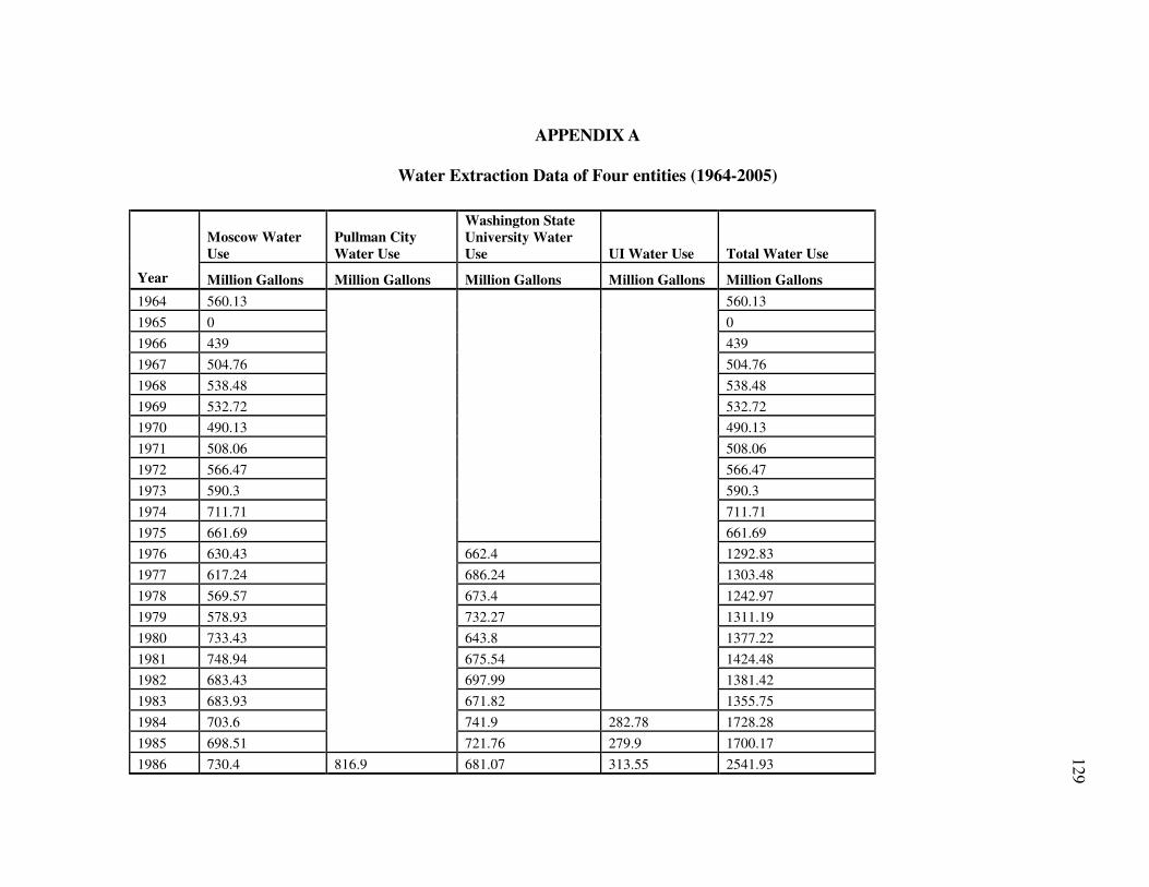
129

APPENDIX A

Water Extraction Data of Four entities (1964-2005)

Moscow Water Use

Pullman City Water Use

Washington State University Water Use UI Water Use Total Water Use

Year Million Gallons Million Gallons Million Gallons Million Gallons Million Gallons

1964 560.13 560.13

1965 0 0

1966 439 439

1967 504.76 504.76

1968 538.48 538.48

1969 532.72 532.72

1970 490.13 490.13

1971 508.06 508.06

1972 566.47 566.47

1973 590.3 590.3

1974 711.71 711.71

1975 661.69 661.69

1976 630.43 662.4 1292.83

1977 617.24 686.24 1303.48

1978 569.57 673.4 1242.97

1979 578.93 732.27 1311.19

1980 733.43 643.8 1377.22

1981 748.94 675.54 1424.48

1982 683.43 697.99 1381.42

1983 683.93 671.82 1355.75

1984 703.6 741.9 282.78 1728.28

1985 698.51 721.76 279.9 1700.17

1986 730.4 816.9 681.07 313.55 2541.93

130

Year Moscow Water Use

Pullman City Water Use

Washington State University Water Use UI Water Use Total Water Use

Million Gallons Million Gallons Million Gallons Million Gallons Million Gallons

1988 713.66 828.72 639.14 365.98 2547.5

1990 753.54 834.42 607.95 350.08 2546

1991 825.91 811.25 601.4 353.4 2591.96

1992 825.64 858.91 604.32 371.67 2660.55

1993 775.73 825.87 605.09 316.4 2523.09

1994 914.4 905.69 648.12 341.13 2809.35

1995 865.67 805.48 584.24 323.34 2578.73

1996 925.21 860.1 592.47 301.68 2679.47

1997 869.93 847.11 560.31 269.4 2546.75

1998 903.56 878.91 571.94 295.35 2649.75

1999 889.1 896.45 573.5 311.9 2670.94

2000 912.74 913.42 576.55 320.8 2723.5

2001 895.1 861.13 627.87 306.6 2690.69

2002 873.43 860.23 585.85 216.81 2536.32

2003 919.52 904.5 608.16 250.13 2682.31

2004 809.27 841.65 557.63 205.59 2414.14

2005 818.96 871.39 515.03 234.63 2440.01

2006 628.33 (Source: UI, WSU, City of Pullman, City of Moscow)

131

APPENDIX B

Comprehensive Data Set of City of Pullman for Economic Analysis

Water extraction

(Single Family)

Total Extraction

Median Household

Income Precipitation Fixed Price

Marginal Price

(Single Family)

Marginal Price (Total Residential)

Housing Unit

(Single family)

Year

Month

ft3 ft3 $ in

Household Size

$ ( 1inch meter size) $ No

Total Households

Total Population

2000 January 1964268 5877889 21662 1.90 2.24 21.930 0.96 0.96 3217 9022 24664

2000 February 1826063 5915316 21696 2.66 2.24 21.930 0.96 0.96 3223 9028 24653

2000 March 2122005 7274413 21731 2.31 2.24 21.930 0.96 0.96 3228 9034 24641

2000 April 1879279 5865495 21765 1.21 2.24 21.930 0.96 0.96 3234 9040 24630

2000 May 2484217 7392175 21799 2.14 2.24 21.930 0.96 0.96 3239 9046 24619

2000 June 3543088 6785373 21833 1.19 2.24 21.930 1.18 1.18 3245 9052 24608

2000 July 5354343 10236314 21867 0.01 2.24 21.930 1.18 1.18 3250 9058 24596

2000 August 7534448 12913743 21902 0.04 2.24 21.930 1.18 1.18 3255 9064 24585

2000 September 5798750 12277019 21936 1.51 2.24 21.930 1.18 1.18 3261 9070 24574

2000 October 2661299 7126734 21970 1.65 2.24 21.930 0.96 0.96 3266 9076 24563

2000 November 2347824 7625634 22004 1.86 2.24 21.930 0.96 0.96 3272 9082 24551

2000 December 1981549 6355439 22038 1.44 2.24 21.930 0.96 0.96 3277 9088 24540

2001 January 2015734 6040603 22073 1.59 2.24 22.920 1.00 1.00 3283 9094 24571

2001 February 1954427 6507531 22107 0.93 2.24 22.920 1.00 1.00 3288 9100 24602

2001 March 1838650 6162655 22141 1.33 2.24 22.920 1.00 1.00 3293 9106 24633

2001 April 2082449 6552777 22175 2.19 2.23 22.920 1.00 1.00 3299 9111 24663

2001 May 2400214 7254617 22209 1.83 2.23 22.920 1.00 1.00 3304 9117 24694

2001 June 3806614 9575364 22244 1.46 2.23 22.920 1.23 1.23 3310 9123 24725

2001 July 5084948 10000424 22278 0.56 2.23 22.920 1.23 1.23 3315 9129 24756

2001 August 5310093 10092392 22312 0.02 2.23 22.920 1.23 1.23 3321 9135 24787

2001 September 7169385 14301170 22346 0.28 2.23 22.920 1.23 1.23 3326 9141 24818

2001 October 3654611 8653608 22380 2.46 2.23 22.920 1.00 1.00 3332 9147 24848

2001 November 2517910 7710475 22415 2.76 2.23 22.920 1.00 1.00 3337 9153 24879

2001 December 1997526 6353920 22449 2.61 2.23 22.920 1.00 1.00 3342 9159 24910

132

Year Month

Water extraction

(Single Family)

Total Extraction

Median Household

Income Precipitation Household

Size Fixed Price

Marginal Price

(Single Family)


Housing Unit

(Single family)

Total Households

Total Population

2002 January 1803846 5191996 22483 2.88 2.23 23.950 1.05 1.05 3348 9165 24943

2002 February 1895084 6254505 22517 1.18 2.23 23.950 1.05 1.05 3353 9171 24975

2002 March 2145152 7467159 22551 0.69 2.23 23.950 1.05 1.05 3359 9177 25008

2002 April 1810296 5694853 22586 0.96 2.23 23.950 1.05 1.05 3364 9183 25040

2002 May 2490631 7493009 22620 1.23 2.23 23.950 1.05 1.05 3370 9189 25073

2002 June 3901991 8544395 22654 1.64 2.23 23.950 1.29 1.29 3375 9195 25105

2002 July 4746682 9344955 22688 0.15 2.23 23.950 1.29 1.29 3380 9201 25138

2002 August 7112037 12889648 22722 0.33 2.23 23.950 1.29 1.29 3386 9207 25170

2002 September 6022030 12204097 22757 0.41 2.23 23.950 1.29 1.29 3391 9213 25203

2002 October 3502139 8531498 22791 0.73 2.23 23.950 1.05 1.05 3397 9219 25235

2002 November 2625739 7974815 22825 1.23 2.23 23.950 1.05 1.05 3402 9225 25268

2002 December 1552390 4890887 22859 2.13 2.23 23.950 1.05 1.05 3408 9231 25300

2003 January 2011543 5790131 22893 4.26 2.23 23.950 1.05 1.05 3413 9237 25350

2003 February 1820444 5159663 22928 1.66 2.23 23.950 1.05 1.05 3418 9243 25401

2003 March 1963734 6423445 22962 4.74 2.23 23.950 1.05 1.05 3424 9249 25451

2003 April 1827297 5881315 22996 1.30 2.23 23.950 1.05 1.05 3429 9255 25502

2003 May 2389655 7634149 23030 1.16 2.23 23.950 1.05 1.05 3435 9261 25552

2003 June 3015584 7045600 23064 0.18 2.23 23.950 1.29 1.29 3440 9267 25603

2003 July 7462948 13653907 23099 0.06 2.23 23.950 1.29 1.29 3446 9273 25653

2003 August 7139747 12717461 23133 0.79 2.23 23.950 1.29 1.29 3451 9279 25703

2003 September 7251902 13935037 23167 0.95 2.23 23.950 1.29 1.29 3456 9285 25754

2003 October 3930321 9179868 23201 0.80 2.22 23.950 1.05 1.05 3462 9290 25804

2003 November 2890490 8496825 23235 2.15 2.22 23.950 1.05 1.05 3467 9296 25855

2003 December 1763475 5524555 23270 3.14 2.22 23.950 1.05 1.05 3473 9302 25905

2004 January 2803937 8227001 23304 6.25 2.22 24.900 1.15 1.15 3478 9308 25851

2004 March 1880474 6048229 23372 1.33 2.22 24.900 1.10 1.10 3489 9320 25744

2004 April 2365776 6880936 23406 1.04 2.22 24.900 1.10 1.10 3494 9326 25691

2004 May 2818361 7675988 23441 3.00 2.22 24.900 1.15 1.15 3500 9332 25637

2004 June 3092558 7166852 23475 0.74 2.22 24.900 1.40 1.30 3505 9338 25584

2004 July 6508931 12149175 23509 0.10 2.22 24.900 1.40 1.40 3511 9344 25530

2004 August 6769112 11822464 23543 1.48 2.22 24.900 1.40 1.40 3516 9350 25476

2004 September 5068512 11253858 23577 1.10 2.22 24.900 1.40 1.40 3522 9356 25423

133

Year Month

Water extraction

(Single Family)

Total Extraction

Median Household

Income Precipitation Household

Size Fixed Price

Marginal Price

(Single Family)


Housing Unit

(Single family)

Total Households

Total Population

2004 October 3340810 8615017 23612 1.72 2.22 24.900 1.40 1.40 3527 9362 25369

2004 November 2119393 6865902 23646 1.76 2.22 24.900 1.10 1.10 3533 9368 25316

2004 December 2064986 6656884 23680 1.36 2.22 24.900 1.10 1.10 3538 9374 25262

2005 January 2091674 5688958 23714 0.91 2.22 25.900 1.14 1.14 3543 9380 25270

2005 February 1976143 6552983 23749 0.10 2.22 25.900 1.14 1.14 3549 9386 25278

2005 March 1925580 6279214 23783 2.33 2.22 25.900 1.14 1.14 3554 9392 25286

2005 April 2162333 6704528 23817 1.53 2.22 25.900 1.14 1.14 3560 9398 25294

2005 May 2437734 7191515 23851 2.74 2.22 25.900 1.14 1.14 3565 9404 25302

2005 June 3142420 6898329 23885 1.25 2.22 25.900 1.46 1.35 3571 9410 25310

2005 July 5649439 10486832 23920 0.39 2.22 25.900 1.46 1.46 3576 9416 25317

2005 August 6689646 11578011 23954 0.17 2.22 25.900 1.46 1.46 3581 9422 25325

2005 September 7420095 14488590 23988 0.28 2.22 25.900 1.82 1.82 3587 9428 25333

2005 October 3679684 8785338 24022 2.28 2.22 25.900 1.46 1.46 3592 9434 25341

2005 November 2394268 7474327 24056 2.44 2.22 25.900 1.14 1.14 3598 9440 25349

2005 December 2200781 6663322 24091 2.56 2.22 25.900 1.14 1.14 3603 9446 25357

2006 January 1956031 5104705 24125 4.35 2.22 26.930 1.19 1.19 3609 9452 25365

2006 February 2108831 7290017 24159 1.33 2.22 26.930 1.19 1.19 3614 9458 25373

2006 April 2164533 6979413 24227 2.51 2.21 26.930 1.19 1.19 3625 9469 25389

2006 May 2480851 7169488 24262 1.45 2.21 26.930 1.19 1.19 3630 9475 25397

2006 June 3862594 8008863 24296 1.75 2.21 26.930 1.51 1.51 3636 9481 25405

2006 July 5963238 10824949 24330 0.10 2.21 26.930 1.51 1.51 3641 9487 25412

2006 August 7133752 11855159 24364 0.14 2.21 26.930 1.51 1.51 3647 9493 25420

`

134

APPENDIX C

Model Development Sections in STELLA Software

Model Home represents the basic information about the models and its navigation setup.

Section 1: Acronyms and Abbreviations represent the acronyms and abbreviations used in the model.

135

136

Section 2: Data -1 Hydrological Data: Precipitation represents the mean areal precipitation of sub-watersheds of surface water watershed. Evapotranspiration represents the mean areal evapotranspiration of sub-watersheds of surface water watershed. Runoff represents the mean areal runoff of sub-watersheds of surface water watershed. Minimum Grande Ronde represents the minimum amount of water that is always stored in Grande Ronde aquifer.

137

Section 2: Data -2 Geographic Data: Total Surface Water Area represents the surface area of six sub-watersheds and their summation. Demographic Data: Population and Water Use represents the current population and per-capita use per day of water in the cities. Average Drawdown Depth represents the present and future potential drawdown depth of the groundwater aquifers.

138

Section 3: Basic Calculation -1 Calculation of Surface Area of Wanapum represents the surface area of Wanapum calculated from aquifer material matrix and thickness of aquifer Surface Area Wanapum groun water region= Volume of Wanapum Aquifer Material Matrix / Thickness of Wanapum Aquifer

Calculation of Surface Area of Grande Ronde represents the surface area of Grande Ronde calculated from aquifer material matrix and thickness of aquifer. Groundwater Area represents total surface area of the Wanapum and Grande Ronde aquifer calculated from Geographical Information System (GIS).

139

Section 3: Basic Calculation -2 Volume of water in Wanapum represents the initial volume of the Wanapum aquifer from groundwater-surface water overlay. It is calculated accordingly. Volume of water in Wanapum Aquifer (V) = Surface Area of Wanapum (A) * Storativity of Aquifer Material Matrix of Wanapum (S)* Draw Dawn Head of

Wanapum (∆H)

Volume of water in Grande Ronde represents the initial volume of the Grande Ronde aquifer from groundwater-surface water overlay. Groundwater volume represents the initial volume of the Wanapum and Grande Ronde aquifer over the entire watershed.

140

Section 4: Model Development -1 Water Demand Forecast, Idaho represents the projected water demand from exponential population growth of cities within Idaho. It is calculated accordingly. Projected final Population (P) = Initial Population (Po) *e

Growth rate ®* Time period (t)

Water Demand Forecast=Projected Population*per capita per day water use*365

Water Demand Forecast, Washington represents the projected exponential population growth of cities within Washington.

141

Section 4: Model Development-2 Simplified Model represents the basic form of surface water and groundwater model where surface water and groundwater regions are not hydrologically separated. Groundwater is divided into Wanapum and Grande Ronde. This setup of the model represents the present scenario of groundwater utilization of Palouse Basin Watershed

142

Section 4: Model Development – 3 Surface Water Hydrology represents the main section of surface water. The water balance was computed over each surface water watershed separately.

143

144

Section 4: Model Development – 4 Groundwater-Surface Water Overlay represents the position of the groundwater regions with respect to the surface water watershed. The recharged water from the surface water watershed reaches to the Wanapum aquifer. Both Wanapum and Grande Ronde aquifers were hydrologically separated into five groundwater regions and assumed to be identical in terms of total surface area.

Palouse

Subregion

Viola

Subregion

Colfax

Subregion

Deep Percolation

Colfax Deep Percolation

Pullman

Deep Percolation

Viola

Pullman

Subregion

Palouse GW

MAC GW1

Voila GWMAC GW2

Deep

Percolated Water

to GR

SFAC GW3

Deep 5 depth

Potlach

Section

PC GW

SFP GW2SFP GW1

SFAC GW2

Potlach area

distribution

Potlach

GW

Deep 2

DepthPalouse area

distribution

Deep

Percolation

Paradise Wanapum

Viola area

distribution

Deep1

depth

MAC area

distribution

MAC

Section

Potlach

Source

Deep

Percolation

SFAC Wanapum

MAC Source

Deep 3

Depth

SFAC GW4

Deep 3

Depth

SFAC GW1

Deep 6 depth

Deep

Percolation

MAC Wanapum

Deep 4

Depth

SFP

Section

SFAC area

Palouse

SFP Source

SFC area

Colfax

PC

Section

Deep

Percolated Water

to GR

Deep

Percolated Water

to GR

PC Source

SFC area Pullman

Deep

Percolation Pullman

Wanapum

SFC area

Moscow

Pullaman area

Moscow

Deep 4

Depth

Deep

Percolation

Palouse Wanapum

Deep 6 depth

Pullman area

Pullman

Deep 4

Depth

Paradise creek area

Moscow

Deep 4

DepthMAC area

Colfax

SFAC

Section

Deep Percolation

Potlach

Palouse

Section

Palouse

source

Deep

Percolation

Potlatch Wanapum

SFAC Source

Deep 4

Depth

Deep

Percolated Water

to GR

Pullman

Region

Viola

Region

Palouse

Region

Colfax

RegionVarification

VarificationTop of Model Development-3

145

Section 5: Groundwater Calculation -1 Groundwater Utilization Present Scenario represents the present scenario of groundwater utilization with hydrologically separated models discussed in Section 4.5.1. At present, Palouse, Viola, Pullman and Colfax solely extract water from the Grande Ronde while Moscow extracts 70% of water from Grande Ronde and the rest from Wanapum.

146

Section 5: Groundwater Calculation -2 Groundwater Utilization without Surface Water represents the management options of Moscow groundwater if surface water utilization is delayed (Section 4.5.1). Even if the water in Moscow Grande Ronde reaches a certain minimum value, still water demand can be fulfilled by Moscow Wanapum. But there is no such option for the Pullman area.

147

Section 5: Groundwater Calculation -3 Groundwater Utilization with Surface Water represents the condition when groundwater is combinedly utilized with surface water. As a default setup, when Moscow Grande Ronde reaches a certain minimum value, then the model automatically manages the water demand by the Moscow Wanapum and surface water systems. For the Pullman area, when Pullman Grande Ronde reaches certain minimum value, the model manages the entire water demand by surface water (Section 4.5.2).

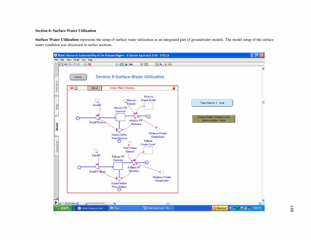
148

Section 6: Surface Water Utilization Surface Water Utilization represents the setup of surface water utilization as an integrated part of groundwater models. The model setup of the surface

water condition was discussed in earlier sections.

149

Section 7: Total Volume- 1 Total recharged Water represents the total amount of recharged water that penetrates from the surface water watershed to the groundwater regions over an entire watershed. Total Demand represents the water demand of the Palouse Basin watershed that includes six cities. Total recharged Water to Wanapum represents the summation of recharge water to the Wanapum groundwater regions from groundwater-surface water overlay.

150

Section 7: Total Volume-2 Total Grande Ronde with Surface Water Utilization represents the total amount of water i.e. stored and recharged water in the Grande Ronde groundwater regions with the surface water utilization setup. Total Groundwater Wanapum represents the total amount of stored and recharged water in the Wanapum groundwater regions from groundwater-surface water overlay. Total Grande Ronde Present Scenario represents the total amount of stored and recharged water in the Grande Ronde groundwater regions in present scenario setup (groundwater-surface water overlay)i.e. without utilization of surface water. Total GR Rate Present Scenario represents the total annual recharge rate to the Grande Ronde in present scenario.

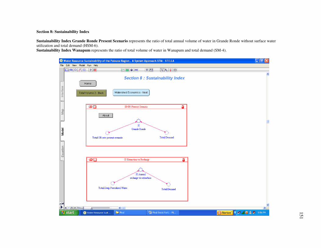
151

Section 8: Sustainability Index Sustainability Index Grande Ronde Present Scenario represents the ratio of total annual volume of water in Grande Ronde without surface water utilization and total demand (HSM-6). Sustainability Index Wanapum represents the ratio of total volume of water in Wanapum and total demand (SM-4).

152

Section 9: Simple Water Demand Economics Simple Water Demand Economics represents the model setup for calculating the total water demand of Pullman area. The multiple regression equation is used to forecast the total water demand per year.

153

Interface Home

Interface Home represents the basic information about the models and its navigation setup.

154

Model Configuration

Model configuration represents the operating unit of the model. In this section, different combinations of switches help to simulate different predefined water resource scenarios. The predefined scenarios are related to the model development phase section of the thesis. The Scenario 1-SM needs all the switches off except bottom a) “Simplified Model”. This predefined condition treats surface water as a single component and same as groundwater. The Scenario 1-HSM needs b) “Groundwater Utilization Present Scenario” switch on and the rest off. In this predefined condition, future scenario of water resource utilizing solely groundwater by Hydrologically Separated Model. The Scenario 2-HSM needs c) “Groundwater Utilization without Surface Water” switch on and the rest off. Moscow groundwater is managed in this predefined condition. The Scenario 3-HSM needs d) “Groundwater Utilization with Surface Water” and e) “Surface Water Utilization” switches on and the rest off. This predefined condition utilizes groundwater combined with surface water. There are altogether ten Numeric Displays in the model configuration section. These tools display the final results of the simulation: the amount of water in aquifers in different scenarios, water demand and population.

155

Model Parameters

Model parameters represent the controller unit of the overall system. The sliders and knobs of this section help to change variable parameters. Two kinds of model parameters are incorporated in this section. The first type is parameters that are either uncertain or where wide range of value exist. The recharge rates, storativity and drawdown depth have a lot of uncertainties. Recharge rates of each sub-watershed can be altered by individual sliders. Another type of parameter like growth rate helps to understand the future water management scenario.

156

APPENDIX D

Equations in Stella

Average Drawdown Depth Average_GR_Drawdown_Depth_Using_Current_Development = (((450-341)+(473-366)+(440-289))/3)/3.28 Average_GR_Drawdown_Using_Future_Development = (((1305-341)+(1458-366)+(1242-289))/3)/3.28 Average_WP_Drawdown_Depth_Using_Current_Infrastructure = (((170-57)+(135-81)+(294-139))/3)/3.28 Average_WP_Drawdown_Depth_Using_Future_Development = (((240-57)+(569-81)+(508-139))/3)/3.28 Calculation of Surface Area of Grand Ronde Colfax_GR_Area = Colfax_GR_Matrix_Volume/Colfax_GR_Thickness*9.290304e-8{Conversion ft2 to km2} Colfax_GR_Matrix_Volume = 2.86E+12{ft3} Colfax_GR_Thickness = 800{ft} Grand_Ronde_Sediment_Volume_ft3 = Colfax_GR_Matrix_Volume+Moscow_GR_Matrix_Volume+Palouse_GR_Matrix_Volume+Pullman_GR_Matrix_Volume+Voila_GR_Matrix_Volume Grand_Ronde_Thickness_ft = (Colfax_GR_Thickness+Moscow_GR_Thickness+Palouse_GR_Thickness+Pullman_GR_Thickness+Voila_GR_Thickness)/6 Moscow_GR_Area = Moscow_GR_Matrix_Volume/Moscow_GR_Thickness*9.290304e-8{Conversion ft2 to km2} Moscow_GR_Matrix_Volume = 5.85E+11{ft3} Moscow_GR_Thickness = 850{ft} Palouse_GR_Area = Palouse_GR_Matrix_Volume/Palouse_GR_Thickness*9.290304e-8{Conversion ft2 to km2} Palouse_GR_Matrix_Volume = 4E+11{ft3} Palouse_GR_Thickness = 500{ft} Pullman_GR_Area = Pullman_GR_Matrix_Volume/Pullman_GR_Thickness*9.290304e-8{Conversion ft2 to km2} Pullman_GR_Matrix_Volume = 2.54E+12{ft3} Pullman_GR_Thickness = 1000{ft} Viola_GR_Area = Voila_GR_Matrix_Volume/Voila_GR_Thickness*9.290304e-8{Conversion ft2 to km2} Voila_GR_Matrix_Volume = 1.83E+11{ft3} Voila_GR_Thickness = 800{ft} Calculation of Surface Area of Wanapum Colfax_Wan_Area = Colfax_Wan_Matrix_Volume/Colfax_Wan_Thickness*9.290304e-8{Conversion ft2 to km2} Colfax_Wan_Matrix_Volume = 1.49E+12{ft3} Colfax_Wan_Thickness = 400{ft} Moscow_Wan_Area = Moscow_Wan_Matrix_Volume/Moscow_Wan_Thickness*9.290304e-8{Conversion ft2 to km2} Moscow_Wan_Matrix_Volume = 3.96E+11{ft3} Moscow_Wan_Thickness = 450{ft}

157

Palouse_Wan_Area = Palouse_Wan_Matrix_Volume/Palouse_Wan_Thickness*9.290304e-8{Conversion ft2 to km2} Palouse_Wan_Matrix_Volume = 5.73E+11{ft3} Palouse_Wan_Thickness = 280{ft} Pullman_Wan_Area = Pullman_Wan_Matrix_Volume/Pullman_Wan_Thickness*9.290304e-8{Conversion ft2 to km2} Pullman_Wan_Matrix_Volume = 4.07E+11{ft3} Pullman_Wan_Thickness = 150{ft} Viola_Wan_Area = Voila_Wan_Matrix_Volume/Voila_Wan_Thickness*9.290304e-8{Conversion ft2 to km2} Voila_Wan_Matrix_Volume = 1.36E+11{ft3} Voila_Wan_Thickness = 450{ft} Wanapum_Sediment_Volume_ft3 = Colfax_Wan_Matrix_Volume+Moscow_Wan_Matrix_Volume+Palouse_Wan_Matrix_Volume+Pullman_Wan_Matrix_Volume+Voila_Wan_Matrix_Volume Wanapum_Thickness_ft = (Colfax_Wan_Thickness+Moscow_Wan_Thickness+Palouse_Wan_Thickness+Pullman_Wan_Thickness+Voila_Wan_Thickness)/6 Evapotranspiration Data ET_13345000 = 538.61/(1000*1000){Conversion mm/yr to km/yr} ET_13345300 = 464.93/(1000*1000){Conversion mm/yr to km/yr} ET_13346100 = 452.23/(1000*1000){Conversion mm/yr to km/yr} ET_13346800 = 497.96/(1000*1000){Conversion mm/yr to km/yr} ET_13348000 = 467.48/(1000*1000){Conversion mm/yr to km/yr} ET_Southfork = 447.15/(1000*1000){Conversion mm/yr to km/yr} Groundwater Areas Total_GR_GW_Area = Colfax_GR_Area+Moscow_GR_Area+Palouse_GR_Area+Pullman_GR_Area+Viola_GR_Area Total_WP_GW_Area = Colfax_Wan_Area+Moscow_Wan_Area+Palouse_Wan_Area+Pullman_Wan_Area+Viola_Wan_Area Groundwater Volume Volume_of_Water__Wanapum_Total = Storativity_Basalt*Total_Surface_Area*Drawdown_Moscow_WP*264172051241.55844 /1000000000{Conversion km3 to billion gallons} Volume_of_Water_Grande_Ronde_Total = Drawdown_Moscow_GR*Storativity_Basalt*Total_Surface_Area*264172051241.55844 /1000000000{Conversion km3 to billion gallons} Population and Water Use Cofax = 150{gallons} Current_Per_Capita_Use = (Cofax+Moscow+Potlatch+Pullman+Viola)/6 Moscow = 180{gallons, 2000 ANNUAL REPORT Water Use in the Palouse Basin Juliet M. McKenna Palouse Basin Aquifer Committee The Palouse Basin Aquifer Committee} Population = Population_Colfax+Population_Moscow+Population_Potlatch+Population_Viola+Population_Pullman Population_Colfax = 2793{2003}

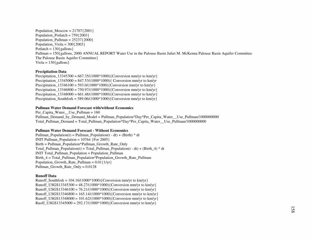
158

Population_Moscow = 21707{2001} Population_Potlatch = 759{2003} Population_Pullman = 25237{2000} Population_Viola = 300{2003} Potlatch = 130{gallons} Pullman = 150{gallons, 2000 ANNUAL REPORT Water Use in the Palouse Basin Juliet M. McKenna Palouse Basin Aquifer Committee The Palouse Basin Aquifer Committee} Viola = 130{gallons} Precipitation Data Percipitation_13345300 = 667.35/(1000*1000){Conversion mm/yr to km/yr} Precipitation_13345000 = 847.53/(1000*1000){ Conversion mm/yr to km/yr Precipitation_13346100 = 593.0/(1000*1000){Conversion mm/yr to km/yr} Precipitation_13346800 = 750.97/(1000*1000){Conversion mm/yr to km/yr} Precipitation_13348000 = 661.48/(1000*1000){Conversion mm/yr to km/yr} Precipitation_Southfork = 589.06/(1000*1000){Conversion mm/yr to km/yr} Pullman Water Demand Forecast with/without Economics Per_Capita_Water__Use_Pullman = 160 Pullman_Demand_by_Demand_Model = Pullman_Population*Day*Per_Capita_Water__Use_Pullman/1000000000 Total_Pullman_Demand = Total_Pullman_Population*Day*Per_Capita_Water__Use_Pullman/1000000000 Pullman Water Demand Forecast - Without Economics Pullman_Population(t) = Pullman_Population(t - dt) + (Birth) * dt INIT Pullman_Population = 10764 {For 2005} Birth = Pullman_Population*Pullman_Growth_Rate_Only Total_Pullman_Population(t) = Total_Pullman_Population(t - dt) + (Birth_4) * dt INIT Total_Pullman_Population = Population_Pullman Birth_4 = Total_Pullman_Population*Population_Growth_Rate_Pullman Population_Growth_Rate_Pullman = 0.01{1/yr} Pullman_Growth_Rate_Only = 0.0128 Runoff Data Runoff_Southfork = 104.16/(1000*1000){Conversion mm/yr to km/yr} Runoff_USGS13345300 = 48.27/(1000*1000){Conversion mm/yr to km/yr} Runoff_USGS13346100 = 76.21/(1000*1000){Conversion mm/yr to km/yr} Runoff_USGS13346800 = 165.14/(1000*1000){Conversion mm/yr to km/yr} Runoff_USGS13348000 = 101.62/(1000*1000){Conversion mm/yr to km/yr} Ruoff_USGS13345000 = 292.17/(1000*1000){Conversion mm/yr to km/yr}

159

Scenario 1 - Groundwater Utilization-Present Scenario Colfax_Grand_Ronde(t) = Colfax_Grand_Ronde(t - dt) + (Recharge_Colfax_Region - Cofax_Extraction) * dt INIT Colfax_Grand_Ronde = Colfax_Volume_GR Recharge_Colfax_Region = Recharge_Colfax Cofax_Extraction = Total_Colfax_Demand Moscow_Grand_Ronde(t) = Moscow_Grand_Ronde(t - dt) + (Recharge_Moscow - Moscow_GR_Extraction) * dt INIT Moscow_Grand_Ronde = Moscow_Volume_GR Recharge_Moscow = (Recharge_to_GR*Moscow_Wan_Area)*264172051241.55844/1000000000{billion gallons/yr} Moscow_GR_Extraction = 0.7*Moscow_Demand{billion gallons/yr} Moscow_Wanapum(t) = Moscow_Wanapum(t - dt) + (Recharge_Combined_Moscow - Recharge_Moscow - Moscow_WP_Extraction) * dt INIT Moscow_Wanapum = Moscow_Volume_Wanapum Recharge_Combined_Moscow = PC_GW+SFAC_GW2+SFP_GW2{billion gallons/yr} Recharge_Moscow = (Recharge_to_GR*Moscow_Wan_Area)*264172051241.55844/1000000000{billion gallons/yr} Moscow_WP_Extraction = 0.3*Moscow_Demand{billion gallons/yr} Palouse_Grand_Ronde(t) = Palouse_Grand_Ronde(t - dt) + (Recharge_Potlach_Region - Palouse_Extraction) * dt INIT Palouse_Grand_Ronde = Palouse_Volume_GR Recharge_Potlach_Region = Recharge_Potlach{billion gallons/yr} Palouse_Extraction = Potlach_Demand{billion gallons/yr} Pullman_Grand_Ronde(t) = Pullman_Grand_Ronde(t - dt) + (Recharge_Pullman_Region - Pullman_Extraction) * dt INIT Pullman_Grand_Ronde = Pullman_Volume_GR Recharge_Pullman_Region = Recharge_Pullman{billion gallons/yr} Pullman_Extraction = Total_Pullman_Demand{billion gallons/yr} Voila_Grand_Ronde(t) = Voila_Grand_Ronde(t - dt) + (Recharge_Viola_Region - Viola_Extraction) * dt INIT Voila_Grand_Ronde = Viola_Volume_GR Recharge_Viola_Region = Recharge_Viola{billion gallons/yr} Viola_Extraction = Viola_Demand{billion gallons/yr} Total_Colfax_Demand = Colfax_Demand+Southfork_Demand Scenario 2 - Groundwater Utilization Without Surface Water Colfax_Grande_Ronde`(t) = Colfax_Grande_Ronde`(t - dt) + (Recharge_Colfax` - Colfax_Extraction`) * dt INIT Colfax_Grande_Ronde` = Colfax_Volume_GR Recharge_Colfax` = Recharge_Colfax{billion gallons/yr} Colfax_Extraction` = Colfax_Demand+Southfork_Demand{billion gallons/yr} Moscow_Grande_Ronde`(t) = Moscow_Grande_Ronde`(t - dt) + (Recharge_Moscow` - Moscow_GR_Extraction`) * dt INIT Moscow_Grande_Ronde` = Moscow_Volume_GR Recharge_Moscow` = (Recharge_to_GR*Moscow_Total_GW_Area)*264172051241.55844/1000000000{billion gallons/yr} Moscow_GR_Extraction` = 0.7*Moscow_Demand{billion gallons/yr} Moscow_Wanapum'(t) = Moscow_Wanapum'(t - dt) + (Combined - Recharge_Moscow` - Moscow_WP_Extraction`) * dt INIT Moscow_Wanapum' = Moscow_Volume_Wanapum Combined = PC_GW+SFAC_GW2+SFP_GW2{billion gallons/yr}

160

Recharge_Moscow` = (Recharge_to_GR*Moscow_Total_GW_Area)*264172051241.55844/1000000000{billion gallons/yr} Moscow_WP_Extraction` = IF(Moscow_Grande_Ronde`<Minimum_Volume_Groundwater)THEN(Moscow_Demand)ELSE(0.3*Moscow_Demand){billion gallons/yr} Palouse_Grande_Ronde`(t) = Palouse_Grande_Ronde`(t - dt) + (Recharge_Potlach` - Palouse_Extraction') * dt INIT Palouse_Grande_Ronde` = Palouse_Volume_GR Recharge_Potlach` = Recharge_Potlach{billion gallons/yr} Palouse_Extraction' = Potlach_Demand{billion gallons/yr} Pullman_Grande_Ronde`(t) = Pullman_Grande_Ronde`(t - dt) + (Recharge_Pullman` - Pullman_Extraction`) * dt INIT Pullman_Grande_Ronde` = Pullman_Volume_GR Recharge_Pullman` = Recharge_Pullman{billion gallons/yr} Pullman_Extraction` = Total_Pullman_Demand{billion gallons/yr} Voila_Grande_Ronde`(t) = Voila_Grande_Ronde`(t - dt) + (Recharge_Viola' - Viola_Extraction`) * dt INIT Voila_Grande_Ronde` = Viola_Volume_GR Recharge_Viola' = Recharge_Viola{billion gallons/yr} Viola_Extraction` = Viola_Demand{billion gallons/yr} Scenario 3 - Groundwater Utilization With Surface Water Colfax_Grande_Ronde''(t) = Colfax_Grande_Ronde''(t - dt) + (Recharge_Colfax`` - Cofax_Extraction'') * dt INIT Colfax_Grande_Ronde'' = Colfax_Volume_GR Recharge_Colfax`` = Recharge_Colfax{billion gallons/yr} Cofax_Extraction'' = Colfax_Demand+Southfork_Demand{billion gallons/yr} Moscow_Grande_Ronde''(t) = Moscow_Grande_Ronde''(t - dt) + (Recharge_Moscow'' - Moscow_GR_Extraction'') * dt INIT Moscow_Grande_Ronde'' = Moscow_Volume_GR Recharge_Moscow'' = (Recharge_to_GR*Moscow_Total_GW_Area)*264172051241.55844/1000000000{billion gallons/yr} Moscow_GR_Extraction'' = IF(Moscow_Grande_Ronde''<Minimum_Volume_Groundwater)THEN(0)ELSE(0.25*Moscow_Demand){billion gallons/yr} Moscow_Wanapum''(t) = Moscow_Wanapum''(t - dt) + (Combined` - Recharge_Moscow'' - Moscow_WP_Extraction'') * dt INIT Moscow_Wanapum'' = Moscow_Volume_Wanapum Combined` = PC_GW+SFAC_GW2+SFP_GW2{billion gallons/yr} Recharge_Moscow'' = (Recharge_to_GR*Moscow_Total_GW_Area)*264172051241.55844/1000000000{billion gallons/yr} Moscow_WP_Extraction'' = IF(Moscow_Grande_Ronde''<Minimum_Volume_Groundwater)THEN(0.5*Moscow_Demand)ELSE(0.30*Moscow_Demand){billion gallons/yr} Palouse_Grande_Ronde''(t) = Palouse_Grande_Ronde''(t - dt) + (Recharge_Potlach`` - Palouse_Extraction'') * dt INIT Palouse_Grande_Ronde'' = Palouse_Volume_GR Recharge_Potlach`` = Recharge_Potlach{billion gallons/yr} Palouse_Extraction'' = Potlach_Demand{billion gallons/yr} Pullman_Grande_Ronde''(t) = Pullman_Grande_Ronde''(t - dt) + (Recharge_Pullman`` - Pullman_GR_Extraction'') * dt INIT Pullman_Grande_Ronde'' = Pullman_Volume_GR Recharge_Pullman`` = Recharge_Pullman{billion gallons/yr} Pullman_GR_Extraction'' = IF(Pullman_Grande_Ronde''<Minimum_Volume_Groundwater)THEN(0)ELSE(0.5*Total_Pullman_Demand){billion gallons/yr}

161

Voila_Grande_Ronde''(t) = Voila_Grande_Ronde''(t - dt) + (Recharge_Viola`` - Viola_Extraction'') * dt INIT Voila_Grande_Ronde'' = Viola_Volume_GR Recharge_Viola`` = Recharge_Viola{billion gallons/yr} Viola_Extraction'' = Viola_Demand{billion gallons/yr} Moscow_Total_GW_Area = 81.614{km2} Scenario I - Simplified Model (SM) Soil(t) = Soil(t - dt) + (Precipitation - Evapotraspiration - Runoff - Recharge_Wanapum_SM) * dt INIT Soil = 0{m^3} Precipitation = (Total_Surface_Area*Precipitation_Depth)*264172051241.55844 /1000000000{Conversion km3/yr to billion gallons/yr} Evapotraspiration = Total_Surface_Area*Evapotraspiration_Depth*264172051241.55844 /1000000000{Conversion km3/yr to billion gallons/yr} Runoff = Total_Surface_Area*Runoff_Depth*264172051241.55844 /1000000000{Conversion km3/yr to billion gallons/yr} Recharge_Wanapum_SM = Precipitation-Evapotraspiration-Runoff Surface_Water_Collection(t) = Surface_Water_Collection(t - dt) + (Runoff) * dt INIT Surface_Water_Collection = 0 Runoff = Total_Surface_Area*Runoff_Depth*264172051241.55844 /1000000000{Conversion km3/yr to billion gallons/yr} Total_Grand_Ronde(t) = Total_Grand_Ronde(t - dt) + (Recharge_GR_SM - Grande_Ronde_Pumpage) * dt INIT Total_Grand_Ronde = Volume_of_Water_Grand_Ronde Recharge_GR_SM = Recharge_to_GR*Total_GW_Area_GR_SM*264172051241.55844 /1000000000{Conversion km3/yr to billion gallons/yr} Grande_Ronde_Pumpage = 0.88*Total_Demand{billion gallons/yr} Total_Wanapum(t) = Total_Wanapum(t - dt) + (Recharge_Wanapum_SM - Wanapum_Pumpage - Recharge_GR_SM) * dt INIT Total_Wanapum = Volume_of_Water_Wanapum Recharge_Wanapum_SM = Precipitation-Evapotraspiration-Runoff Wanapum_Pumpage = 0.12*Total_Demand{billion gallons/yr} Recharge_GR_SM = Recharge_to_GR*Total_GW_Area_GR_SM*264172051241.55844 /1000000000{Conversion km3/yr to billion gallons/yr} Evapotraspiration_Depth = 495.42/(1000*1000){Km/yr} Precipitation_Depth = 709.413/(1000*1000){Km/yr} Runoff_Depth = 172.76/(1000*1000){km/yr} Total_GW_Area_GR_SM = 768.83{km2} SI Extraction vs Recharge SI_Annual__recharge_vs_extraction = (Total_Demand/Total_Deep_Percolated_Water)*100 SI GR Present Scenario SI__Grande_Ronde = (Total_Demand/Total_GR_Rate_Present_Scenario)*100 Surface Water Groundwater Overlay Colfax_Subregion(t) = Colfax_Subregion(t - dt) + (MAC_GW2 + SFAC_GW1 - Recharge_Colfax) * dt INIT Colfax_Subregion = Colfax_Volume_Wanapum MAC_GW2 = Recharge_3_Depth*MAC_area_Colfax{billion gallons/yr}

162

SFAC_GW1 = Recharge_4_Depth*SFC_area_Colfax{billion gallons/yr} Recharge_Colfax = (Colfax_Wan_Area*Recharge_to_GR)*264172051241.55844/1000000000{Conversion km3 to billion gallons} MAC_Section(t) = MAC_Section(t - dt) + (MAC_Source - MAC_GW1 - MAC_GW2) * dt INIT MAC_Section = 0 MAC_Source = Recharge_MAC_WP_Wanapum{billion gallons/yr} MAC_GW1 = Recharge_3_Depth*MAC_area_distribution{billion gallons/yr} MAC_GW2 = Recharge_3_Depth*MAC_area_Colfax{billion gallons/yr} Palouse_Section(t) = Palouse_Section(t - dt) + (Palouse_Source - Palouse_GW) * dt INIT Palouse_Section = 0 Palouse_Source = Recharge_Palouse_WP{billion gallons/yr} Palouse_GW = Recharge_2_Depth*Palouse_area_distribution{billion gallons/yr} Palouse_Subregion(t) = Palouse_Subregion(t - dt) + (Potlach_GW + Palouse_GW + MAC_GW1 + SFAC_GW4 - Recharge_Potlach) * dt INIT Palouse_Subregion = Palouse_Volume_Wanapum Potlach_GW = Recharge_1_Depth*Potlach_area_distribution{billion gallons/yr} Palouse_GW = Recharge_2_Depth*Palouse_area_distribution{billion gallons/yr} MAC_GW1 = Recharge_3_Depth*MAC_area_distribution{billion gallons/yr} SFAC_GW4 = Recharge_4_Depth*SFAC_area_Palouse{billion gallons/yr} Recharge_Potlach = (Recharge_to_GR*Palouse_Wan_Area)*264172051241.55844/1000000000{Conversion km3 to billion gallons} PC_Section(t) = PC_Section(t - dt) + (PC_Source - PC_GW) * dt INIT PC_Section = 0 PC_Source = Recharge_Paradise_WP{billion gallons/yr} PC_GW = Recharge_5_depth*Paradise_creek_area_Moscow{billion gallons/yr} Potlach_Section(t) = Potlach_Section(t - dt) + (Potlach_Source - Potlach_GW) * dt INIT Potlach_Section = 0 Potlach_Source = Recharge_Potlatch_WP_Wanapum{billion gallons/yr} Potlach_GW = Recharge_1_Depth*Potlach_area_distribution{billion gallons/yr} Pullman_Subregion(t) = Pullman_Subregion(t - dt) + (SFAC_GW3 + SFP_GW1 - Recharge_Pullman) * dt INIT Pullman_Subregion = Pullman_Volume_Wanapum SFAC_GW3 = Recharge_4_Depth*SFC_area_Pullman{billion gallons/yr} SFP_GW1 = Recharge_6_depth*Pullman_area_Pullman{billion gallons/yr} Recharge_Pullman = (Recharge_to_GR*Pullman_Wan_Area)*264172051241.55844/1000000000{Conversion km3 to billion gallons} SFAC_Section(t) = SFAC_Section(t - dt) + (SFAC_Source - SFAC_GW1 - SFAC_GW4 - Voila_GW - SFAC_GW2 - SFAC_GW3) * dt INIT SFAC_Section = 0 SFAC_Source = Recharge_SFAC_WP{billion gallons/yr} SFAC_GW1 = Recharge_4_Depth*SFC_area_Colfax{billion gallons/yr} SFAC_GW4 = Recharge_4_Depth*SFAC_area_Palouse{billion gallons/yr} Voila_GW = Recharge_4_Depth*Viola_area_distribution{billion gallons/yr} SFAC_GW2 = Recharge_4_Depth*SFC_area_Moscow{billion gallons/yr} SFAC_GW3 = Recharge_4_Depth*SFC_area_Pullman{billion gallons/yr} SFP_Section(t) = SFP_Section(t - dt) + (SFP_Source - SFP_GW1 - SFP_GW2) * dt

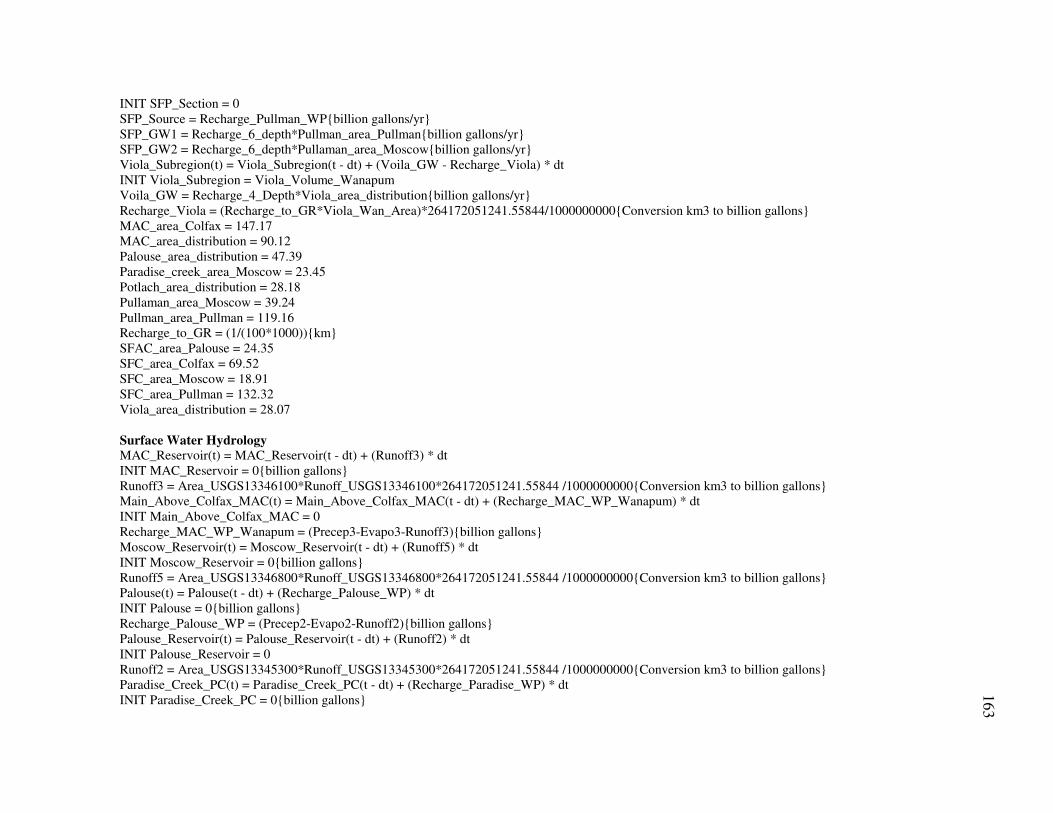
163

INIT SFP_Section = 0 SFP_Source = Recharge_Pullman_WP{billion gallons/yr} SFP_GW1 = Recharge_6_depth*Pullman_area_Pullman{billion gallons/yr} SFP_GW2 = Recharge_6_depth*Pullaman_area_Moscow{billion gallons/yr} Viola_Subregion(t) = Viola_Subregion(t - dt) + (Voila_GW - Recharge_Viola) * dt INIT Viola_Subregion = Viola_Volume_Wanapum Voila_GW = Recharge_4_Depth*Viola_area_distribution{billion gallons/yr} Recharge_Viola = (Recharge_to_GR*Viola_Wan_Area)*264172051241.55844/1000000000{Conversion km3 to billion gallons} MAC_area_Colfax = 147.17 MAC_area_distribution = 90.12 Palouse_area_distribution = 47.39 Paradise_creek_area_Moscow = 23.45 Potlach_area_distribution = 28.18 Pullaman_area_Moscow = 39.24 Pullman_area_Pullman = 119.16 Recharge_to_GR = (1/(100*1000)){km} SFAC_area_Palouse = 24.35 SFC_area_Colfax = 69.52 SFC_area_Moscow = 18.91 SFC_area_Pullman = 132.32 Viola_area_distribution = 28.07 Surface Water Hydrology MAC_Reservoir(t) = MAC_Reservoir(t - dt) + (Runoff3) * dt INIT MAC_Reservoir = 0{billion gallons} Runoff3 = Area_USGS13346100*Runoff_USGS13346100*264172051241.55844 /1000000000{Conversion km3 to billion gallons} Main_Above_Colfax_MAC(t) = Main_Above_Colfax_MAC(t - dt) + (Recharge_MAC_WP_Wanapum) * dt INIT Main_Above_Colfax_MAC = 0 Recharge_MAC_WP_Wanapum = (Precep3-Evapo3-Runoff3){billion gallons} Moscow_Reservoir(t) = Moscow_Reservoir(t - dt) + (Runoff5) * dt INIT Moscow_Reservoir = 0{billion gallons} Runoff5 = Area_USGS13346800*Runoff_USGS13346800*264172051241.55844 /1000000000{Conversion km3 to billion gallons} Palouse(t) = Palouse(t - dt) + (Recharge_Palouse_WP) * dt INIT Palouse = 0{billion gallons} Recharge_Palouse_WP = (Precep2-Evapo2-Runoff2){billion gallons} Palouse_Reservoir(t) = Palouse_Reservoir(t - dt) + (Runoff2) * dt INIT Palouse_Reservoir = 0 Runoff2 = Area_USGS13345300*Runoff_USGS13345300*264172051241.55844 /1000000000{Conversion km3 to billion gallons} Paradise_Creek_PC(t) = Paradise_Creek_PC(t - dt) + (Recharge_Paradise_WP) * dt INIT Paradise_Creek_PC = 0{billion gallons}

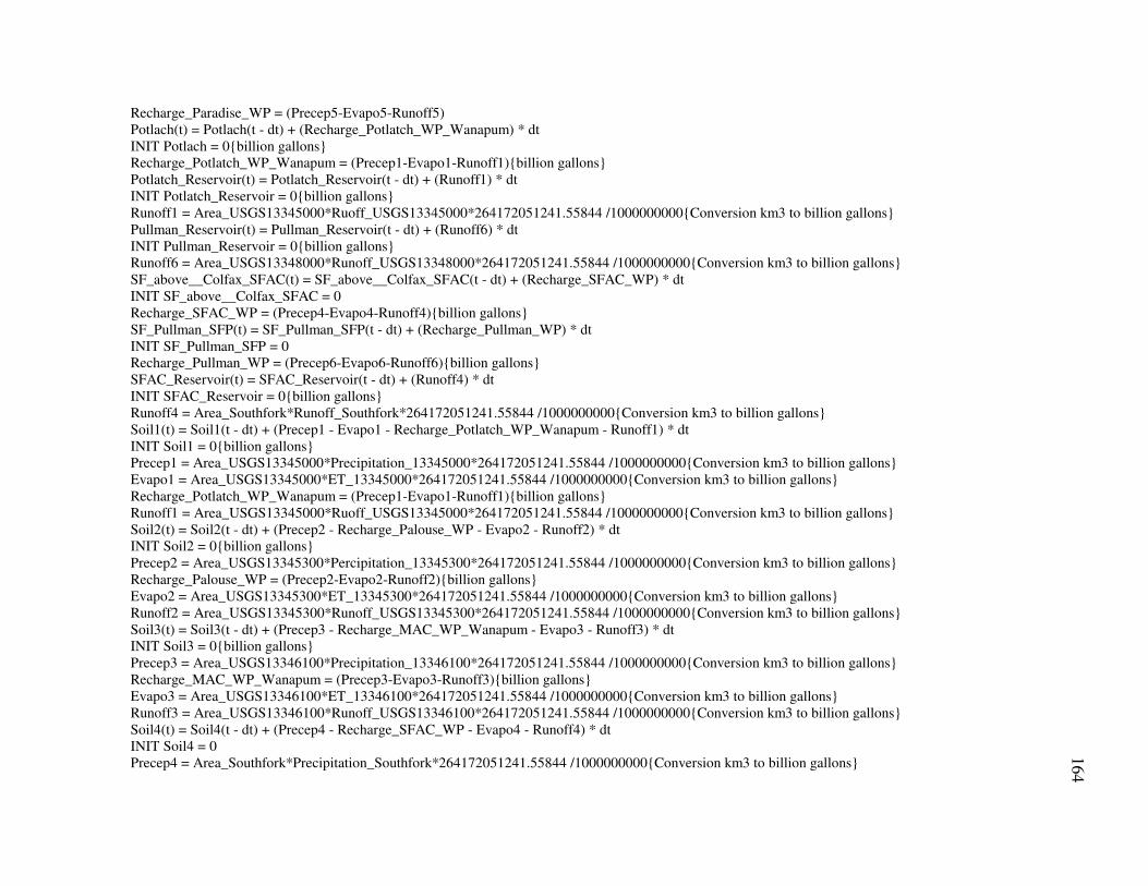
164

Recharge_Paradise_WP = (Precep5-Evapo5-Runoff5) Potlach(t) = Potlach(t - dt) + (Recharge_Potlatch_WP_Wanapum) * dt INIT Potlach = 0{billion gallons} Recharge_Potlatch_WP_Wanapum = (Precep1-Evapo1-Runoff1){billion gallons} Potlatch_Reservoir(t) = Potlatch_Reservoir(t - dt) + (Runoff1) * dt INIT Potlatch_Reservoir = 0{billion gallons} Runoff1 = Area_USGS13345000*Ruoff_USGS13345000*264172051241.55844 /1000000000{Conversion km3 to billion gallons} Pullman_Reservoir(t) = Pullman_Reservoir(t - dt) + (Runoff6) * dt INIT Pullman_Reservoir = 0{billion gallons} Runoff6 = Area_USGS13348000*Runoff_USGS13348000*264172051241.55844 /1000000000{Conversion km3 to billion gallons} SF_above__Colfax_SFAC(t) = SF_above__Colfax_SFAC(t - dt) + (Recharge_SFAC_WP) * dt INIT SF_above__Colfax_SFAC = 0 Recharge_SFAC_WP = (Precep4-Evapo4-Runoff4){billion gallons} SF_Pullman_SFP(t) = SF_Pullman_SFP(t - dt) + (Recharge_Pullman_WP) * dt INIT SF_Pullman_SFP = 0 Recharge_Pullman_WP = (Precep6-Evapo6-Runoff6){billion gallons} SFAC_Reservoir(t) = SFAC_Reservoir(t - dt) + (Runoff4) * dt INIT SFAC_Reservoir = 0{billion gallons} Runoff4 = Area_Southfork*Runoff_Southfork*264172051241.55844 /1000000000{Conversion km3 to billion gallons} Soil1(t) = Soil1(t - dt) + (Precep1 - Evapo1 - Recharge_Potlatch_WP_Wanapum - Runoff1) * dt INIT Soil1 = 0{billion gallons} Precep1 = Area_USGS13345000*Precipitation_13345000*264172051241.55844 /1000000000{Conversion km3 to billion gallons} Evapo1 = Area_USGS13345000*ET_13345000*264172051241.55844 /1000000000{Conversion km3 to billion gallons} Recharge_Potlatch_WP_Wanapum = (Precep1-Evapo1-Runoff1){billion gallons} Runoff1 = Area_USGS13345000*Ruoff_USGS13345000*264172051241.55844 /1000000000{Conversion km3 to billion gallons} Soil2(t) = Soil2(t - dt) + (Precep2 - Recharge_Palouse_WP - Evapo2 - Runoff2) * dt INIT Soil2 = 0{billion gallons} Precep2 = Area_USGS13345300*Percipitation_13345300*264172051241.55844 /1000000000{Conversion km3 to billion gallons} Recharge_Palouse_WP = (Precep2-Evapo2-Runoff2){billion gallons} Evapo2 = Area_USGS13345300*ET_13345300*264172051241.55844 /1000000000{Conversion km3 to billion gallons} Runoff2 = Area_USGS13345300*Runoff_USGS13345300*264172051241.55844 /1000000000{Conversion km3 to billion gallons} Soil3(t) = Soil3(t - dt) + (Precep3 - Recharge_MAC_WP_Wanapum - Evapo3 - Runoff3) * dt INIT Soil3 = 0{billion gallons} Precep3 = Area_USGS13346100*Precipitation_13346100*264172051241.55844 /1000000000{Conversion km3 to billion gallons} Recharge_MAC_WP_Wanapum = (Precep3-Evapo3-Runoff3){billion gallons} Evapo3 = Area_USGS13346100*ET_13346100*264172051241.55844 /1000000000{Conversion km3 to billion gallons} Runoff3 = Area_USGS13346100*Runoff_USGS13346100*264172051241.55844 /1000000000{Conversion km3 to billion gallons} Soil4(t) = Soil4(t - dt) + (Precep4 - Recharge_SFAC_WP - Evapo4 - Runoff4) * dt INIT Soil4 = 0 Precep4 = Area_Southfork*Precipitation_Southfork*264172051241.55844 /1000000000{Conversion km3 to billion gallons}

165

Recharge_SFAC_WP = (Precep4-Evapo4-Runoff4){billion gallons} Evapo4 = Area_Southfork*ET_Southfork*264172051241.55844 /1000000000{Conversion km3 to billion gallons} Runoff4 = Area_Southfork*Runoff_Southfork*264172051241.55844 /1000000000{Conversion km3 to billion gallons} Soil5(t) = Soil5(t - dt) + (Precep5 - Recharge_Paradise_WP - Evapo5 - Runoff5) * dt INIT Soil5 = 0{billion gallons} Precep5 = Area_USGS13346800*Precipitation_13346800*264172051241.55844 /1000000000{Conversion km3 to billion gallons} Recharge_Paradise_WP = (Precep5-Evapo5-Runoff5) Evapo5 = Area_USGS13346800*ET_13346800*264172051241.55844 /1000000000{Conversion km3 to billion gallons} Runoff5 = Area_USGS13346800*Runoff_USGS13346800*264172051241.55844 /1000000000{Conversion km3 to billion gallons} Soil6(t) = Soil6(t - dt) + (Precep6 - Recharge_Pullman_WP - Evapo6 - Runoff6) * dt INIT Soil6 = 0{billion gallons} Precep6 = Area_USGS13348000*Precipitation_13348000*264172051241.55844 /1000000000{Conversion km3 to billion gallons} Recharge_Pullman_WP = (Precep6-Evapo6-Runoff6){billion gallons} Evapo6 = Area_USGS13348000*ET_13348000*264172051241.55844 /1000000000{Conversion km3 to billion gallons} Runoff6 = Area_USGS13348000*Runoff_USGS13348000*264172051241.55844 /1000000000{Conversion km3 to billion gallons} Recharge_1_Depth = Recharge_Potlatch_WP_Wanapum/Area_USGS13345000{km} Recharge_2_Depth = Recharge_Palouse_WP/Area_USGS13345300{km} Recharge_3_Depth = Recharge_MAC_WP_Wanapum/Area_USGS13346100{km} Recharge_4_Depth = Recharge_SFAC_WP/Area_Southfork{km} Recharge_5_depth = Recharge_Paradise_WP/Area_USGS13346800{km} Recharge_6_depth = Recharge_Pullman_WP/Area_USGS13348000{km} Surface Water Utilization Moscow_SW_Reservoir(t) = Moscow_SW_Reservoir(t - dt) + (Runoff_Moscow - Moscow_SW_Extraction - Unused_Surface_Water_Moscow) * dt INIT Moscow_SW_Reservoir = 0 Runoff_Moscow = 0.8*Runoff5{billion gallons/yr} Moscow_SW_Extraction = IF(Moscow_Grande_Ronde''<Minimum_Volume_Groundwater)THEN(0.5*Moscow_Demand)ELSE(0.45*Moscow_Demand){billion gallons/yr} Unused_Surface_Water_Moscow = Runoff_Moscow-Moscow_SW_Extraction Pullman_SW_Reservoir(t) = Pullman_SW_Reservoir(t - dt) + (Runoff_Pullman - Pullman_SW__Extraction - Unused_Surface_Water_Pullman) * dt INIT Pullman_SW_Reservoir = 0 Runoff_Pullman = 0.8*Runoff6{billion gallons/yr} Pullman_SW__Extraction = IF(Pullman_Grande_Ronde''<Minimum_Volume_Groundwater)THEN(Total_Pullman_Demand)ELSE(0.5*Total_Pullman_Demand){billion gallons/yr} Unused_Surface_Water_Pullman = Runoff_Pullman-Pullman_SW__Extraction Total Demand Total_Demand = Colfax_Demand+Moscow_Demand+Potlach_Demand+Southfork_Demand+Viola_Demand+Total_Pullman_Demand{billion gallons/yr} Total GR Rate Present Scenario

166

Total_GR_Rate_Present_Scenario = Recharge_Colfax+Recharge_Moscow+Recharge_Potlach+Recharge_Pullman+Recharge_Viola Total Grand Ronde with Surface Water Utilization Total_GR_with_Surface_Water_Utilization = Recharge_Colfax``+Recharge_Potlach``+Recharge_Pullman``+Recharge_Viola``+Combined` Total Grand Ronde Present Scenario Total_GR_Present_Scenario = Colfax_Grand_Ronde+Moscow_Grand_Ronde+Palouse_Grand_Ronde+Pullman_Grand_Ronde+Voila_Grand_Ronde Total Groundwater Wanapum Total_Ground_Water__Upper_Aquifer = Colfax_Subregion+Moscow_Wanapum+Palouse_Subregion+Pullman_Subregion+Viola_Subregion Total Population Total_Population = Main_Above_Colfax_Population+Moscow_Population+Potlatch_Population+Total_Pullman_Population+Southfork_Above_Colfax_Population+Viola_Population Total Recharged Water Total_Deep_Percolated_Water = Recharge_Pullman_WP+Recharge_MAC_WP_Wanapum+Recharge_Palouse_WP+Recharge_Paradise_WP+Recharge_Potlatch_WP_Wanapum+Recharge_SFAC_WP Total Recharged Water to Wanapum Colfax_Wanapum_Recharge = MAC_GW2+SFAC_GW1{billion gallons/yr} Moscow_Wanapum_Recharge = PC_GW+SFAC_GW2+SFP_GW2{billion gallons/yr} Palouse_Wanapum_Recharge = MAC_GW1+Palouse_GW+Potlach_GW+SFAC_GW4{billion gallons/yr} Pullman_Wanapum_Recharge = SFAC_GW3+SFP_GW1{billion gallons/yr} Total_Recharged_Water_Wanapum = Colfax_Wanapum_Recharge+Moscow_Wanapum_Recharge+Palouse_Wanapum_Recharge+Pullman_Wanapum_Recharge+Viola_Wanapum_Recharge{billion gallons/yr} Viola_Wanapum_Recharge = Voila_GW{billion gallons/yr} Total Surface Water Area Area_Southfork = 439038000/(1000*1000){Conversion mm2 to km2} Area_USGS13345000 = 816369000/(1000*1000){Conversion mm2 to km2} Area_USGS13345300 = 69772700/(1000*1000){Conversion mm2 to km2} Area_USGS13346100 = 388455000/(1000*1000){Conversation mm2 to km2} Area_USGS13346800 = 45653200/(1000*1000){Conversion mm2 to km2} Area_USGS13348000 = 284356000/(1000*1000){Conversion mm2 to km2} Total_Surface_Area = Area_USGS13345000+Area_USGS13345300+Area_USGS13346100+Area_Southfork+Area_USGS13346800+Area_USGS13348000{km2}

167

Volume of Water in Grand Ronde from Groundwater-Surface Water Overlay Colfax_Volume_GR = Colfax_GR_Area*Drawdown_Colfax_GR*Storativity_Basalt*264172051241.55844 /1000000000{Conversion km3 to billion gallons} Drawdown_Colfax_GR = 800/(3.28*1000){Conversion ft to km} Drawdown_Moscow_GR = 890/(3.28*1000){Conversion ft to km} Drawdown_Palouse_GR = 499/(3.28*1000){Conversion ft to km} Drawdown_Pullman_GR = 528/(3.28*1000){Conversion ft to km} Drawdown_Voila_GR = 800/(3.28*1000){Conversion ft to km} Moscow_Volume_GR = Drawdown_Moscow_GR*Moscow_GR_Area*Storativity_Basalt*264172051241.55844 /1000000000{Conversion km3 to billion gallons} Palouse_Volume_GR = Drawdown_Palouse_GR*Palouse_GR_Area*Storativity_Basalt*264172051241.55844 /1000000000{Conversion km3 to billion gallons} Pullman_Volume_GR = Drawdown_Pullman_GR*Pullman_GR_Area*Storativity_Basalt*264172051241.55844 /1000000000{Conversion km3 to billion gallons} Storativity_Basalt = 0.0001 Viola_Volume_GR = Drawdown_Voila_GR*Storativity_Basalt*Viola_GR_Area*264172051241.55844 /1000000000{Conversion km3 to billion gallons} Volume_of_Water_Grand_Ronde = Moscow_Volume_GR+Pullman_Volume_GR+Viola_Volume_GR+Palouse_Volume_GR+Colfax_Volume_GR Volume of Water in Wanapum from Groundwater- Surface Water Overlay Colfax_Volume_Wanapum = Colfax_Wan_Area*Drawdown_Colfax_WP*Storativity_Basalt*264172051241.55844 /1000000000{Conversion km3 to billion gallons} Drawdown_Colfax_WP = 0 Drawdown_Moscow_WP = 243/(3.28*1000){Conversion ft to km} Drawdown_Palouse_WP = 0 Drawdown_Pullman_WP = 0/(3.28*1000){Conversion ft to km} Drawdown_Voila_WP = 0 Moscow_Volume_Wanapum = Drawdown_Moscow_WP*Moscow_Wan_Area*Storativity_Basalt*264172051241.55844 /1000000000{Conversion km3 to billion gallons} Palouse_Volume_Wanapum = Drawdown_Palouse_WP*Palouse_Wan_Area*Storativity_Basalt*264172051241.55844 /1000000000{Conversion km3 to billion gallons} Pullman_Volume_Wanapum = Drawdown_Pullman_WP*Pullman_Wan_Area*Storativity_Basalt*264172051241.55844 /1000000000{Conversion km3 to billion gallons} Viola_Volume_Wanapum = Drawdown_Voila_WP*Storativity_Basalt*Viola_Wan_Area*264172051241.55844 /1000000000{Conversion km3 to billion gallons} Volume_of_Water_Wanapum = Moscow_Volume_Wanapum+Pullman_Volume_Wanapum+Viola_Volume_Wanapum+Palouse_Volume_Wanapum+Colfax_Volume_Wanapum Water Demand Economics Average_Number_of_People_per_Household = -0.004*TIME+10.24

168

Fixed_Price = 0.7658*TIME-1509.9 Households = 71.6*TIME-134184 Marginal_Price = 0.0527*TIME-104.45 Median_Household_Income = 410.42*TIME-799212 Per_Capita_Per_Day_Water_Use_Regression = Pullman_Demand_by_Economic_Module*1000000000/(Total_Pullman_Population*365) Precipitation_Inch = 27.92 Pullman_Demand_by_Economic_Module = (Marginal_Price^1.6*Fixed_Price^-5.07*Precipitation_Inch^-0.048*Average_Number_of_People_per_Household^188.72*Median_Household_Income^24.32*EXP(-377))*100*7.481*Households*12/1000000000 Water Demand Forecast, Idaho Moscow_Population(t) = Moscow_Population(t - dt) + (Birth_1) * dt INIT Moscow_Population = Population_Moscow Birth_1 = Moscow_Population*Population_Growth_Rate_Moscow Potlatch_Population(t) = Potlatch_Population(t - dt) + (Birth_3) * dt INIT Potlatch_Population = Population_Potlatch Birth_3 = Potlatch_Population*Population_Growth_Rate_Potlach Viola_Population(t) = Viola_Population(t - dt) + (Birth_2) * dt INIT Viola_Population = Population_Viola Birth_2 = Viola_Population*Population_Growth_Rate_Viola Day = 365{days} Moscow_Demand = (Moscow_Population*Day*Per_Capita_Use_Moscow)/1000000000{Conversion gallons to billion gallons} Per_Capita_Use_Moscow = 160{gallons} Per_Capita_Use_Potlach = 160{gallons} Per_Capita_Use_Viola = 160{gallons} Population_Growth_Rate_Moscow = 0.01{1/yr} Population_Growth_Rate_Potlach = 0.01{1/yr} Population_Growth_Rate_Viola = 0.01{1/yr} Potlach_Demand = (Potlatch_Population*Day*Per_Capita_Use_Potlach)/1000000000{Conversion gallons to billion gallons} Viola_Demand = (Viola_Population*Day*Per_Capita_Use_Viola)/1000000000{Conversion gallons to billion gallons} Water Demand Forecast, Washington Main_Above_Colfax_Population(t) = Main_Above_Colfax_Population(t - dt) + (Birth_6) * dt INIT Main_Above_Colfax_Population = Population_Colfax/2 Birth_6 = Main_Above_Colfax_Population*Population_Growth_Rate_MAC Southfork_Above_Colfax_Population(t) = Southfork_Above_Colfax_Population(t - dt) + (Birth_5) * dt INIT Southfork_Above_Colfax_Population = Population_Colfax/2 Birth_5 = Southfork_Above_Colfax_Population*Population_Growth__Rate_SFAC Colfax_Demand = (Main_Above_Colfax_Population*Day*Per_Capita_Use_MAC)/1000000000{Conversion gallons to billion gallons} Per_Capita_Use_MAC = 160{gallons} Per_Capita_Use_SFAC = 160{gallons}

169

Population_Growth__Rate_SFAC = 0.01{1/yr} Population_Growth_Rate_MAC = 0.01{1/yr} Southfork_Demand = (Southfork_Above_Colfax_Population*Day*Per_Capita_Use_SFAC)/1000000000{Conversion gallons to billion gallons} Not in a sector Minimum_Volume_Groundwater = 1{Billion}

170

APPENDIX E

3D Projection of Palouse Basin Groundwater Surface Water Overlay