Embed Size (px)
Citation preview

Flood Hydraulics project for the course Flood Risk Evaluation
Prof. Alessio Radice
Group Members v Seyed Mohammad Sadegh (Arshia) Mousavi (836154) v Abdolreza Khalili (832669) v Omid Habibzadeh Bigdarvish (836722)

General Presentation
The Serio (Lombard: Sère[1][2]) is an Italian river that flows entirely within Lombardy, crossing the provinces of Bergamo and Cremona. It is 124 kilometres (77 mi) long and flows into the Adda at Bocca di Serio south of Crema.Its valley is known as the Val Seriana.

3 General Presentation
General information
• Length: 125 km
• Area of basin: 1250 km2
• Average discharge: around 25 m3/s
• Water used for hydropower (famous falls are activated some times every year) and irrigation
Our models examines the last 15 km of the river, from Crema to the confluence with the Adda. Data provided:
• Cross sections (map and survey data)
• Flood hydrograph
• Geometry data incorporated into a project of Hec‐Ras
• Pictures of the reach

4 1-D Modeling – Introduction

5
Objective: 1‐D modeling of river flow in ordinary and peak conditions.
Steps:�
² Cross section data: choosing extent of main channel and roughness values for main channel and floodplains
² Completing geometry data: adding the bridge at section 6.1² Choosing discharge data and boundary conditions² Choosing levees² Running models:
v Steady model with ordinary flow: Sensitivity analysis (roughness and BCs) and discussion
v Steady model with peak flow: Sensitivity analysis (geometry, levees, roughness, BCs) and discussion
v Unsteady model for 200-year hydrograph: Sensitivity analysis (outflow + storage, single or multiple) and discussion
1-D Modeling - Theoretical

6
Theoretical Background
HEC-RAS as an 1-D modeling software is based on the Saint Venant Equations. These equations are obtained based on the following assumptions, generally satisfied in hydraulic processes: o flow is one-dimensional. o All the quantities can be described as continuous and derivable functions of longitudinal position
(s) and time (t). o Fluid is uncompressible. o Flow is gradually varied, and the pressure is distributed hydrostatically. o Bed slope is small enough to consider cross sections as vertical. o Channel is prismatic in shape. o Flow is fully turbulent.
Saint Venant Equations:
1-D Modeling - Theoretical

7
For special cases, these equations can be simplified as follows: § Steady flow with no temporal variation:
§ Steady flow with no spatial and temporal variability (Uniform flow):
In case of steady flow, modeling is simple: a constant discharge should be assign to the entire reach, and a boundary condition for water level which would be at upstream for supercritical flows or at downstream for subcritical flows.
1-D Modeling - Theoretical

8
Energy Head Loss
The change in the energy head between adjacent sections equals the head loss. The head loss occurring between two cross-sections is consisting of the sum of the frictional losses and expansion or contraction losses.
The energy head is given by:
1-D Modeling - Theoretical

9
In case of unsteady flow, an initial condition is necessary together with an upstream boundary condition (usually a discharge hydrograph) and a second boundary condition which must be upstream for supercritical flows or downstream for subcritical flow.
Characteristic Depths
Critical Depth dc: The depth for which the specific energy is minimum is called the critical depth. When dc>d the flow is called supercritical (velocity larger than that for critical flow). When dc<d the flow is subcritical.
1-D Modeling - Theoretical

10
Normal Depth d0:
If no quantity varies with the longitudinal direction, the flow is called uniform, and the momentum equation representing the process is S0=Sf. The depth for which this happens is called the normal depth.
For a given discharge, Sf is a decreasing function of water depth, therefore:
d>d0 ⇒S0 >Sf d<d0 ⇒S0 <Sf
1-D Modeling - Theoretical

11
Steady model for the ordinary flow
Length: 125 km�
Average discharge: 25 m3/s
S0= 0.15%
1-D Modeling Description

12 1-D Modeling Description

13
Main channel bank stationsThe left and the right bank values are inserted in the HEC-RAS software considering the width of the channel in the map and trying to find the nodes having roughly the same distance.
1-D Modeling Description

14
Manning Roughness Coefficient:
There is no exact method for selecting n values. At the present stage of knowledge to select a value of n actually means to estimate the resistance to flow in a given channel which is really a matter of intangibles.
So for this issue, different individuals will obtain different results, such as:
1. experience; comparison with similar systems 2. calibration over past (and known) events 3. sensitivity analysis
For the Calibration of the main channel, left and right banks of the channel we considered the USGS data for the rivers.
1-D Modeling Description

15
Manning Coefficient:
² The values of roughness for main channel, left and right banks are selected based on the map of the area and provided pictures of the sections. These values are obtained from the “Verified Roughness Characteristics of Natural Channels” provided by USGS website.
² The Manning coefficient of main channel has been selected n=0.038 whereas for the sensitivity analysis considered n=0.028 and n=0.041.
² In addition, different manning values have been observed for the three cases with respect to the Hec-Ras software’s table.
1-D Modeling Description
Serio River Clark Fork River
USGS
N=0.028

16
Manning Coefficient (n) in Flood Plains:Left and Right Coefficients bank corresponding to n=0.028
1-D Modeling Description
Left%Bank 0.035 Light%Brush%&%tress%in%winterRight%Bank 0.035 Light%Brush%&%tress%in%winterLeft%Bank 0.035 Light%Brush%&%tress%in%winterRight%Bank 0.025 Short%GrassLeft%Bank 0.035 Light%Brush%&%tress%in%winterRight%Bank 0.025 Short%GrassLeft%Bank 0.025 Short%GrassRight%Bank 0.08 Heavy%stand%of%timber,%Few%down%treesLeft%Bank 0.035 Light%Brush%&%tress%in%winterRight%Bank 0.08 Heavy%stand%of%timber,%Few%down%treesLeft%Bank 0.035 Light%Brush%&%tress%in%winterRight%Bank 0.035 Light%Brush%&%tress%in%winterLeft%Bank 0.025 Short%GrassRight%Bank 0.025 Short%GrassLeft%Bank 0.028Right%Bank 0.028Left%Bank 0.028Right%Bank 0.028Left%Bank 0.025 Short%GrassRight%Bank 0.035 Light%Brush%&%tress%in%winterLeft%Bank 0.035 Light%Brush%&%tress%in%winterRight%Bank 0.025 Short%GrassLeft%Bank 0.035 Light%Brush%&%tress%in%winterRight%Bank 0.035 Light%Brush%&%tress%in%winterLeft%Bank 0.035 Light%Brush%&%tress%in%winterRight%Bank 0.035 Light%Brush%&%tress%in%winter
6.15
7
Bridge%Sections%(Main%Channel%value)
8
8.1
8.2
5
6
6.05
2.1
3
4
1
2
Sections Left / Right Bank Value Description
Left%Bank 0.025 Short%GrassRight%Bank 0.035 Light%Brush%&%tress%in%winterLeft%Bank 0.035 Light%Brush%&%tress%in%winterRight%Bank 0.035 Light%Brush%&%tress%in%winterLeft%Bank 0.025 Short%GrassRight%Bank 0.035 Light%Brush%&%tress%in%winterLeft%Bank 0.045 Medium%to%dense%brushRight%Bank 0.025 Short%GrassLeft%Bank 0.045 Medium%to%dense%brushRight%Bank 0.035 Light%Brush%&%tress%in%winterLeft%Bank 0.05 Cleared%land%with%tree%stumps%but%heavy%sproutsRight%Bank 0.05 Cleared%land%with%tree%stumps%but%heavy%sproutsLeft%Bank 0.05 Cleared%land%with%tree%stumps%but%heavy%sproutsRight%Bank 0.05 Cleared%land%with%tree%stumps%but%heavy%sproutsLeft%Bank 0.05 Cleared%land%with%tree%stumps%but%heavy%sproutsRight%Bank 0.05 Cleared%land%with%tree%stumps%but%heavy%sproutsLeft%Bank 0.05 Cleared%land%with%tree%stumps%but%heavy%sproutsRight%Bank 0.05 Cleared%land%with%tree%stumps%but%heavy%sproutsLeft%Bank 0.035 Light%Brush%&%tress%in%winterRight%Bank 0.035 Light%Brush%&%tress%in%winterLeft%Bank 0.045 Medium%to%dense%brushRight%Bank 0.035 Light%Brush%&%tress%in%winterLeft%Bank 0.035 Light%Brush%&%tress%in%winterRight%Bank 0.035 Light%Brush%&%tress%in%winterLeft%Bank 0.035 Light%Brush%&%tress%in%winterRight%Bank 0.035 Light%Brush%&%tress%in%winterLeft%Bank 0.035 Light%Brush%&%tress%in%winterRight%Bank 0.035 Light%Brush%&%tress%in%winter
15.1
20
16
17
18
19
13
14
15
11
12
12.1
Value Description
9
10
Sections Left / Right Bank

17
Manning Coefficient (n) in Flood Plains:Left and Right Coefficients bank corresponding to n=0.038
1-D Modeling Description
Left%Bank 0.05 Light%Brush%&%tress%in%winterRight%Bank 0.05 Light%Brush%&%tress%in%winterLeft%Bank 0.05 Light%Brush%&%tress%in%winterRight%Bank 0.03 Short%GrassLeft%Bank 0.05 Light%Brush%&%tress%in%winterRight%Bank 0.03 Short%GrassLeft%Bank 0.03 Short%GrassRight%Bank 0.1 Heavy%stand%of%timber,%Few%down%treesLeft%Bank 0.05 Light%Brush%&%tress%in%winterRight%Bank 0.1 Heavy%stand%of%timber,%Few%down%treesLeft%Bank 0.05 Light%Brush%&%tress%in%winterRight%Bank 0.05 Light%Brush%&%tress%in%winterLeft%Bank 0.03 Short%GrassRight%Bank 0.03 Short%GrassLeft%Bank 0.038Right%Bank 0.038Left%Bank 0.038Right%Bank 0.038Left%Bank 0.03 Short%GrassRight%Bank 0.05 Light%Brush%&%tress%in%winterLeft%Bank 0.05 Light%Brush%&%tress%in%winterRight%Bank 0.03 Short%GrassLeft%Bank 0.05 Light%Brush%&%tress%in%winterRight%Bank 0.05 Light%Brush%&%tress%in%winterLeft%Bank 0.05 Light%Brush%&%tress%in%winterRight%Bank 0.05 Light%Brush%&%tress%in%winter
Bridge%Sections%(Main%Channel%value)
Sections Left / Right Bank Value Description
1
2
2.1
3
4
5
8.2
8.1
6
6.05
6.15
7
8
Left%Bank 0.03 Short%GrassRight%Bank 0.05 Light%Brush%&%tress%in%winterLeft%Bank 0.05 Light%Brush%&%tress%in%winterRight%Bank 0.03 Light%Brush%&%tress%in%winterLeft%Bank 0.05 Short%GrassRight%Bank 0.03 Light%Brush%&%tress%in%winterLeft%Bank 0.03 Medium%to%dense%brushRight%Bank 0.1 Short%GrassLeft%Bank 0.05 Medium%to%dense%brushRight%Bank 0.1 Light%Brush%&%tress%in%winterLeft%Bank 0.05 Cleared%land%with%tree%stumps%but%heavy%sproutsRight%Bank 0.05 Cleared%land%with%tree%stumps%but%heavy%sproutsLeft%Bank 0.03 Cleared%land%with%tree%stumps%but%heavy%sproutsRight%Bank 0.03 Cleared%land%with%tree%stumps%but%heavy%sproutsLeft%Bank 0.038 Cleared%land%with%tree%stumps%but%heavy%sproutsRight%Bank 0.038 Cleared%land%with%tree%stumps%but%heavy%sproutsLeft%Bank 0.038 Cleared%land%with%tree%stumps%but%heavy%sproutsRight%Bank 0.038 Cleared%land%with%tree%stumps%but%heavy%sproutsLeft%Bank 0.038 Light%Brush%&%tress%in%winterRight%Bank 0.038 Light%Brush%&%tress%in%winterLeft%Bank 0.03 Medium%to%dense%brushRight%Bank 0.05 Light%Brush%&%tress%in%winterLeft%Bank 0.05 Light%Brush%&%tress%in%winterRight%Bank 0.03 Light%Brush%&%tress%in%winterLeft%Bank 0.05 Light%Brush%&%tress%in%winterRight%Bank 0.05 Light%Brush%&%tress%in%winterLeft%Bank 0.05 Light%Brush%&%tress%in%winterRight%Bank 0.05 Light%Brush%&%tress%in%winter
14
15
15.1
16
Left / Right Bank Value Description
9
10
13
Sections
11
12
12.1
17
18
19
20

18
Manning Coefficient (n) in Flood Plains:Left and Right Coefficients bank corresponding to n=0.041
1-D Modeling Description
Left%Bank 0.06 Light%Brush%&%tress%in%winterRight%Bank 0.06 Light%Brush%&%tress%in%winterLeft%Bank 0.06 Light%Brush%&%tress%in%winterRight%Bank 0.035 Short%GrassLeft%Bank 0.06 Light%Brush%&%tress%in%winterRight%Bank 0.035 Short%GrassLeft%Bank 0.035 Short%GrassRight%Bank 0.12 Heavy%stand%of%timber,%Few%down%treesLeft%Bank 0.06 Light%Brush%&%tress%in%winterRight%Bank 0.12 Heavy%stand%of%timber,%Few%down%treesLeft%Bank 0.06 Light%Brush%&%tress%in%winterRight%Bank 0.06 Light%Brush%&%tress%in%winterLeft%Bank 0.035 Short%GrassRight%Bank 0.035 Short%GrassLeft%Bank 0.041Right%Bank 0.041Left%Bank 0.041Right%Bank 0.041Left%Bank 0.035 Short%GrassRight%Bank 0.06 Light%Brush%&%tress%in%winterLeft%Bank 0.06 Light%Brush%&%tress%in%winterRight%Bank 0.035 Short%GrassLeft%Bank 0.06 Light%Brush%&%tress%in%winterRight%Bank 0.06 Light%Brush%&%tress%in%winterLeft%Bank 0.035 Light%Brush%&%tress%in%winterRight%Bank 0.06 Light%Brush%&%tress%in%winter
6.15
7
Bridge%Sections%(Main%Channel%value)
8
8.1
8.2
5
6
6.05
2.1
3
4
1
2
Sections Left / Right Bank Value DescriptionLeft%Bank 0.035 Short%GrassRight%Bank 0.06 Light%Brush%&%tress%in%winterLeft%Bank 0.06 Light%Brush%&%tress%in%winterRight%Bank 0.06 Light%Brush%&%tress%in%winterLeft%Bank 0.035 Short%GrassRight%Bank 0.06 Light%Brush%&%tress%in%winterLeft%Bank 0.11 Medium%to%dense%brushRight%Bank 0.035 Short%GrassLeft%Bank 0.11 Medium%to%dense%brushRight%Bank 0.06 Light%Brush%&%tress%in%winterLeft%Bank 0.08 Cleared%land%with%tree%stumps%but%heavy%sproutsRight%Bank 0.08 Cleared%land%with%tree%stumps%but%heavy%sproutsLeft%Bank 0.08 Cleared%land%with%tree%stumps%but%heavy%sproutsRight%Bank 0.08 Cleared%land%with%tree%stumps%but%heavy%sproutsLeft%Bank 0.08 Cleared%land%with%tree%stumps%but%heavy%sproutsRight%Bank 0.08 Cleared%land%with%tree%stumps%but%heavy%sproutsLeft%Bank 0.08 Cleared%land%with%tree%stumps%but%heavy%sproutsRight%Bank 0.08 Cleared%land%with%tree%stumps%but%heavy%sproutsLeft%Bank 0.06 Light%Brush%&%tress%in%winterRight%Bank 0.06 Light%Brush%&%tress%in%winterLeft%Bank 0.11 Medium%to%dense%brushRight%Bank 0.06 Light%Brush%&%tress%in%winterLeft%Bank 0.06 Light%Brush%&%tress%in%winterRight%Bank 0.06 Light%Brush%&%tress%in%winterLeft%Bank 0.06 Light%Brush%&%tress%in%winterRight%Bank 0.06 Light%Brush%&%tress%in%winterLeft%Bank 0.06 Light%Brush%&%tress%in%winterRight%Bank 0.06 Light%Brush%&%tress%in%winter
15.1
20
16
17
18
19
13
14
15
11
12
12.1
Value Description
9
10
Sections Left / Right Bank

19 1-D Modeling Description
Serio River
Manning Coefficient (n) in Flood Plains:Left and Right Coefficients bank corresponding to n=0.028

20 1-D Modeling Description
Manning Coefficient (n) in Flood Plains:Left and Right Coefficients bank corresponding to n=0.038
Serio RiverMoyie River

21 1-D Modeling Description
Manning Coefficient (n) in Flood Plains:Left and Right Coefficients bank corresponding to n=0.041
Middle Fork River Serio River

22
Floodplain
Section 1
1-D Modeling Description

23
Bridge: v At the section 6.1, a bridge is added to the channel. v We accomplished this by adding one section to the upstream, one section to downstream and one
section at the location of the structure.v The total width of the bridge is 10m.v The distance between these three sections (6.05-6.1-6.15) is10m from the middle section of the
bridge.
1-D Modeling Steady – Ordinary Flow

24 1-D Modeling Steady – Ordinary Flow
BridgeCreate a section before (6.15) Create a section after (6.05)Delete section 6.1�Insert the bridge (6.1)

25 Ordinary Flow
Bridge Section (Sec. 6.1)

26
Limitations Considerations of 1D Modeling v Since HEC-RAS is a 1D modeling software, it cannot consider whether water can move
across the main channel to the flood plains or not. Therefore, if the bed elevation at floodplain is lower than water surface, HEC-RAS will consider water flows into the flood plains. And in this case levee should be added to the section. For this issue, we have considered both view 3D multiple cross section plot and view cross sections.
v In ordinary flow (Q=25 m^3/sec), there are two necessity to add levees in Sections 2 and 8_1, after adding these levees water does not exist in the flood plains.
v The presence of levees is specially required for the steady peak flow and the unsteady simulation based on 200 years hydrograph.
1-D Modeling Description

27 1-D Modeling Description
Adding Levee in Section 2
3D View
Cross Section View

28
Levee
Cross Section View
3D View
1-D Modeling Description
Section 2(After adding Levee)

29 1-D Modeling Description
Adding Levee in Section 8.1As can be seen, in the section 8.1, a levee is added to the right of the main channel. Since HEC-RAS is a 1-D modeling software, it cannot consider whether water can move across the main channel to the banks or not. Thus, if the water surface is higher than the bed elevation at the floodplain water, HEC-RAS will consider water flows into the banks. To avoid this issue, in the section 8.1 in our model, a levee has to be added.

30 1-D Modeling Description
Section 8.1(After adding Levee)
Section 8.1(Before adding Levee)

31 1-D Modeling Description – Ordinary Flow
Overall 3D View after adding levee (All Sections )

32
Boundary ConditionsØ The discharge for the ordinary flow is 25 m3/s.
Ø The boundary conditions for the river depend on the nature of the flow. In the case of subcritical flow, we have to input just downstream condition and for supercritical flows, just upstream condition is needed.
Ø By running the model with some assumed boundary conditions (critical flow at upstream and normal flow at downstream), it was noted that the Froude Number along the channel is lower than 1. Therefore, the flow is subcritical and just downstream boundary condition has to be set. To do so, a sensitivity analysis of the boundary condition need to be done.
Ø For the Reference scenario we have chosen the normal depth for the downstream and Critical depth for the upstream.
1-D Modeling Description
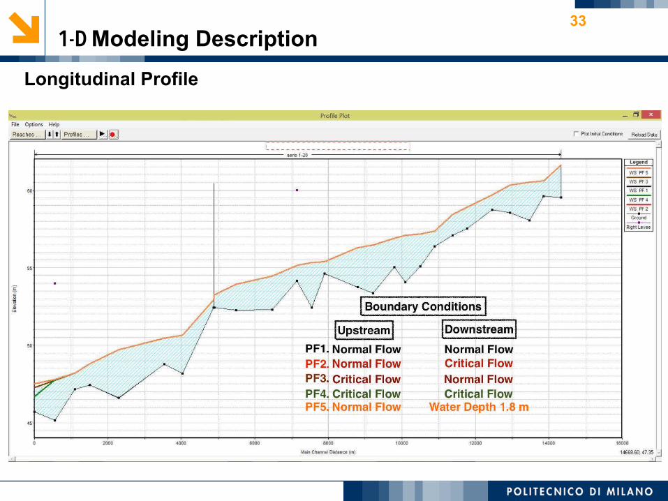
33 1-D Modeling Description
Longitudinal Profile

34 Ordinary Flow
3D View (without Flood)

35 Ordinary Flow
Bridge Section (Sec. 6.1)

36 Ordinary Flow
Bridge Section (Sec. 6.1)
The contraction in the bridge section causes the flow depth to change. Since the flow is subcritical, water elevation decreases after the bridge and gets close to the critical depth.

37 Ordinary Flow
Sensitivity Analysis for Boundary Condition
To check the sensitivity of the results with respect to the boundary conditions, 5 sets of boundary conditions are considered and their results are compared:
�1. Upstream Normal flow and Downstream Normal flow (S=0.0015)
2. Upstream Normal flow and Downstream Critical flow �
3. Upstream Critical flow and Downstream Normal flow (S=0.0015) (Reference Scenario)
4. Upstream Critical flow and Downstream Critical flow
5. Upstream Normal flow and Downstream fixed Water Surface Elevation: 47.51
(45.71 Bed Elevation + 1.8 m Water Depth)

38 1-D Modeling Description
Water Surface for different boundary conditions

39 Ordinary Flow
Results: Velocity Conditions Noticeable rise in water velocity in cases 2 and 4 (water level tends to critical depth)
Velocity for different boundary conditions

40 Ordinary Flow
Sensitivity Analysis for Boundary Condition
Results
1. In whole profile (except bridge section) different boundary condition in upstream makes no change in water profile. Because water level is over critical depth in whole reach (subcritical flow) and just in case of a supercritical flow upstream boundary condition affect our water profile.
2. At this project (subcritical flow) the downstream boundary condition affect the water profile. Water level variation is occurred in the last 4 stations (downstream).

41 Ordinary Flow
Roughness Sensitivity Analysis
In applying the Manning number the greatest difficulty lies in the determination of the roughness coefficient n; there is no exact method of selecting the n value. In the present study, comparison with similar system of the other rivers has been carried out based on the database: “Verified Roughness Characteristics of Natural Channels” provided by USGS website. ︎In ordinary flow water exists only in main channel therefore the simulation is only dependent on the manning coefficient of main channel and not left and right banks. Therefore for flood plains same manning coefficient has been chosen. ︎To study the roughness sensitivity, the manning coefficients are once increased from n=0.038 (reference coefficient) to n=0.041 and once decreased from n=0.038 to 0.028
The roughness sensitivity is evaluated regarding two aspects: In this analysis two aspects have been considered:v Water Surface elevationv Velocity

42 Ordinary Flow
Roughness Sensitivity Analysis
v Water Surface elevationv Velocity
Considering the graph provided, it is easy to observe that by increasing the manning coefficient (n), the water surface elevation is raised. However, generally speaking different manning coefficient values (n), have provided almost the same water surface elevation compared to the dimension of our channel. This hypothesis will be examined later in this project.
An important point of this graph, is the behavior seen at the location of the bridge. It is clear that regardless of the magnitude of the manning coefficient, the water surface elevation approach to the same level for all conditions. This may indicate that in this specific location, due to the contraction caused by the bridge piers, a critical condition has occurred. Checking the Fr=1 in this location verifies this speculation. The results obtained from the HEC-RAS model verifies that the flow is subcritical before and after this location while, when the flow reaches the bridge, the flow is critical.

43 Ordinary Flow
Profile Output Table for reference scenario

44 Ordinary Flow
Sensitivity Analysis for Boundary Condition
Results: Water SurfaceNoticeable rise in water velocity in cases 2 and 4 (water level tends to critical depth)

45 Ordinary Flow
Roughness Sensitivity Analysis
v Water Surface elevationv Velocity
Two points can we concluded from the velocity graph.
1. The graph with higher Manning’s value causes lower velocity as expected.
2. The increase in roughness results in the rise of the water surface elevation. The higher water surface elevation yield lower velocity of the flow.

46 Ordinary Flow
Velocity sensitivity analysis

47 Peak Flow
v Average discharge 561.12 m3/s (based on peak value of 200 –year hydrograph)
Levees
² 13 sections need adding levees to control flood plain.
² Criteria for deciding whether to add levee or not:
1. Considering the residential areas and facilities close to the flood plain.
2. If the bed elevation is lower than water surface HEC-RAS will consider this
area as a flooded area, so levees are required to avoid this issue.
Peak Flow Properties

48 Peak Flow
Adding Levee Section 20
Before Levee
After Levee

49 Peak Flow
Adding Levee Section 18
Before Levee
After Levee

50 Peak Flow
Adding Levee Section 17
Before Levee
After Levee

51 Peak Flow
Adding Levee Section 16
Before Levee
After Levee

52 Peak Flow
Adding Levee Section 14
Before Levee
After Levee

53 Peak Flow
Adding Levee Section 13
Before Levee
After Levee

54 Peak Flow
Adding Levee Section 12
Before Levee
After Levee

55 Peak Flow
Adding Levee Section 11
Before Levee
After Levee

56 Peak Flow
Adding Levee Section 5
Before Levee
After Levee

57 Peak Flow
Adding Levee Section 4
Before Levee
After Levee

58 Peak Flow
Adding Levee
Section 3
Before Levee
After Levee

59 Peak Flow
Adding Levee
Section 2
Before Levee
After Levee

60 Peak Flow
Adding Levee Section 1
Before Levee
After Levee
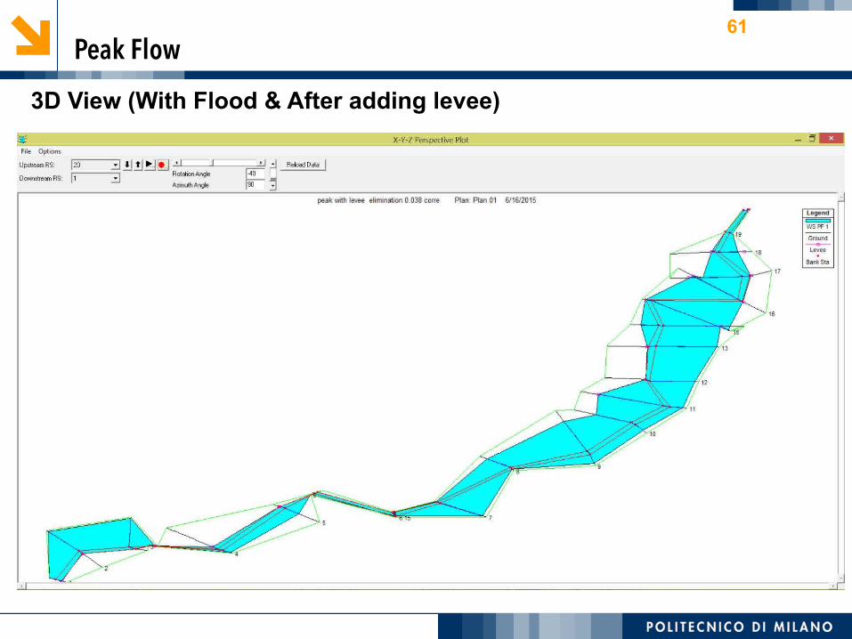
61 Peak Flow
3D View (With Flood & After adding levee)

62 Peak Flow
Sensitivity analysis in case of adding levee and omitting cross sections

63 Peak Flow
Sensitivity analysis in case of adding levee and eliminating cross sections
Section Elevation Difference16 0.313 0.49 0.2
Differences in water elevation
Comparing the graphs and the results of the two sets of data:1. No elimination of cross sections and No levees.2. With levees and eliminating some cross sections.We can observe that in the upstream sections (16, 13, 9) of the eliminated cross sections (15.1, 12.1, 8.2, 8.1) the elevation of the water is increased after adding the levees and eliminating the mentioned cross sections by the values provided in the above table.
mmm

64 Peak Flow
Sensitivity analysis in case of adding levee and eliminating cross sections
Comparing the graphs and the results of the two sets of data:1. No levees and No elimination in cross sections.2. With levees, No eliminating cross sections.We can observe that the graph belonging to the case of no levee and no elimination is always lower or equal to the one related to the case of having levees but no elimination in cross sections.
Comparing the graphs and the results of the two sets of data:1. No levees and with elimination of cross sections.2. With levees, No eliminating cross sections.One could notice that by eliminating the cross sections (case 1) the water surface level would decrease.
65 Peak Flow
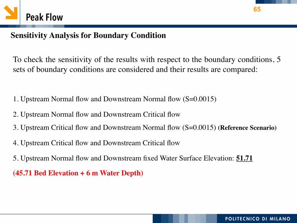
Sensitivity Analysis for Boundary Condition
To check the sensitivity of the results with respect to the boundary conditions, 5 sets of boundary conditions are considered and their results are compared:
�1. Upstream Normal flow and Downstream Normal flow (S=0.0015)
2. Upstream Normal flow and Downstream Critical flow �
3. Upstream Critical flow and Downstream Normal flow (S=0.0015) (Reference Scenario)
4. Upstream Critical flow and Downstream Critical flow
5. Upstream Normal flow and Downstream fixed Water Surface Elevation: 51.71
(45.71 Bed Elevation + 6 m Water Depth)
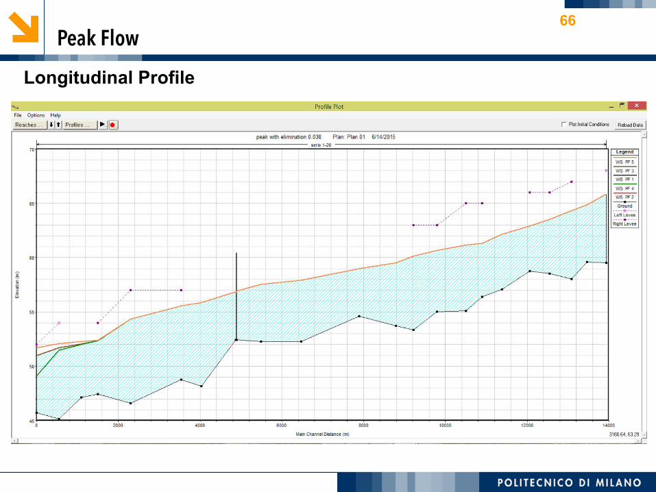
66 Peak Flow
Longitudinal Profile

67 Peak Flow
Velocity

68 Peak Flow
Sensitivity Analysis for Boundary Condition
Results
One could observe that different boundary condition would result in the same velocity
except in the case of sections in the downstream of the river in which the difference is due
to the different boundary conditions applied there.

69 Peak Flow
Roughness Sensitivity Analysis
In applying the Manning number the greatest difficulty lies in the determination of the roughness coefficient n; there is no exact method of selecting the n value. In the present study, comparison with similar system of the other rivers has been carried out based on the database: “Verified Roughness Characteristics of Natural Channels” provided by USGS website. ︎In the peak flow water is not only flowing in the main channel as it was in the case of ordinary flow explained earlier. Left and right bank also contain a portion of water flow so different manning coefficient in the banks is also applied.︎
The roughness sensitivity is evaluated regarding two aspects: In this analysis two aspects have been considered:v Water Surface elevationv Velocity

70 Peak Flow
Roughness Sensitivity Analysis
v Water Surface elevationv Velocity
For this type of flow, the result obtained in the case of ordinary flow are true. Moreover, it is
clear that regardless of the magnitude of the manning coefficient, the water surface elevation
approach to the same level for all conditions for the bridge section. Moreover it is observed
that the water surface along the channel is always above the critical depth. Meaning that
there is subcritical flow in the whole channel.

71 Peak Flow
Roughness Sensitivity Analysis
v Water Surface elevation

72 Peak Flow
Roughness Sensitivity Analysis
v Water Surface elevationv Velocity
Two points can we concluded from the velocity graph.
1. The graph with higher Manning’s value causes lower velocity as expected.
2. The increase in roughness results in the rise of the water surface elevation. The higher
water surface elevation yield lower velocity of the flow.

73 Peak Flow
Roughness Sensitivity Analysis
v Water Surface elevationv Velocity

74 Peak Flow
Roughness Sensitivity Analysis
Results:�
q ︎︎While the difference in the water surface elevation and velocity of both peak and ordinary flow in the case of different (n) values is relatively small, we could observe that the difference in the case of peak flow is larger. In the other words, peak flow results are more sensitive to manning coefficient.
q To conclude, one could state that to use the manning coefficient considering the similar river sections of the USGS and predict the case of river Serio, is acceptable.

75 Unsteady Model
Unsteady model for 200-year Hydrograph To model for the unsteady flow, all the parameters from steady models are used. In this case different flow rates is considered for different sections of the river based on the excel sheet provided.
§ Model conditions§ Boundary condition�
Upstream: 200-year hydrograph�Downstream: normal depth with slope of 0.0015
§ Initial condition� Initial discharge

76 Unsteady Model
Unsteady flow data The original dataset is interpolated with 60 minute time interval. This time interval is small enough with respect to the whole event history ( 200 years).

77
Longitudinal Profile of the corrected geometry
Unsteady Flow

78 Unsteady flow
3D View (Flooded Areas):

79 Unsteady Model
40
42
44
46
48
50
52
54
56
58
60
62
64
66
68
0 2000 4000 6000 8000 10000 12000 14000 16000
Steady Vs. Unsteady flow
bed
steady flow
unsteady flow
Comparison: Steady and Unsteady elevation analysis (at max. water profile)
80
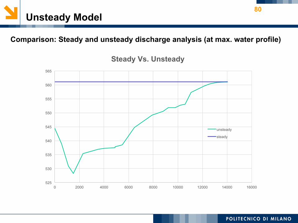
Comparison: Steady and unsteady discharge analysis (at max. water profile)
Unsteady Model
525
530
535
540
545
550
555
560
565
0 2000 4000 6000 8000 10000 12000 14000 16000
Steady Vs. Unsteady
unsteady
steady

81
0
0.5
1
1.5
2
2.5
3
3.5
0 2000 4000 6000 8000 10000 12000 14000 16000
steady Vs. Unsteady
unsteady
steady
Comparison: Steady and unsteady velocity analysis (at max. water profile)
Unsteady Model

82 Unsteady Model
Results:
v It can be observed that the maximum difference between the steady and unsteady flow discharge values is 5.87 percent. This amount shows the loss of Q by considering unsteady type of flow.
v The values of discharge, velocity and water surface elevation are relatively similar in the case of analyzing Serio river. This could be explained by the fact that the difference between steady and unsteady values is dominant only if the channel profile is long enough.

83 Two Dimensional (2D) Modeling
Theoretical Background

84 Two Dimensional (2D) Modeling
Theoretical Background

85 Two Dimensional (2D) Modeling
Theoretical BackgroundThe 2D model depth averaged, mass and momentum conservation equations are:
The bed shear stress are computed by: The turbulent normal and shear stresses are computed according to the Boussinesq’s assumption as:

86 Two Dimensional (2D) Modeling
Benefits
Ø ︎Ability to model more complex flows including floodplain and underground flows
Ø ︎Ability to consider impact of obstructions. Ø ︎ No need to force the geometry to be appropriate
for modeling
Limitationsv If the phenomenon is abrupt, the 1D model
contains discontinuities that water would hardly follow.
v ︎Results are limited by the accuracy of the assumptions, input data and the computing power of the computer program.
v Modeling complexity and precision are not a substitute for sound engineering judgment

87 Two Dimensional (2D) Modeling
Comparing the results of 2-D with 1D
Since River 2D results 2 values for velocity along the X and Y axes,
and computes the water depth at each node, it is not possible to have
single longitudinal profiles for velocity and water surface for the river.
Therefore, the results are compared section by section

88 Two Dimensional (2D) Modeling
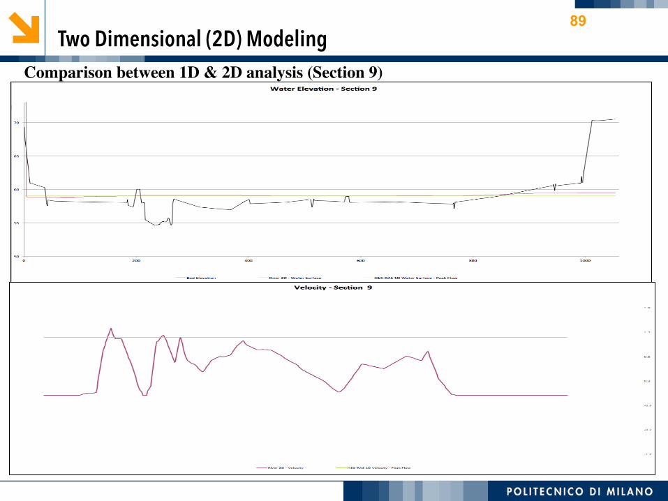
89 Two Dimensional (2D) Modeling
Comparison between 1D & 2D analysis (Section 9)

90 Two Dimensional (2D) Modeling
Comparison between 1D & 2D analysis (Section 10)

91 Two Dimensional (2D) Modeling
Comparison between 1D & 2D analysis (Section 11)

92 Two Dimensional (2D) Modeling
Comparison between 1D & 2D analysis (Section 12)

93 Two Dimensional (2D) Modeling
Comparison between 1D & 2D analysis (Section 13)

94 Two Dimensional (2D) Modeling
Comparison between 1D & 2D analysis (Section 14)
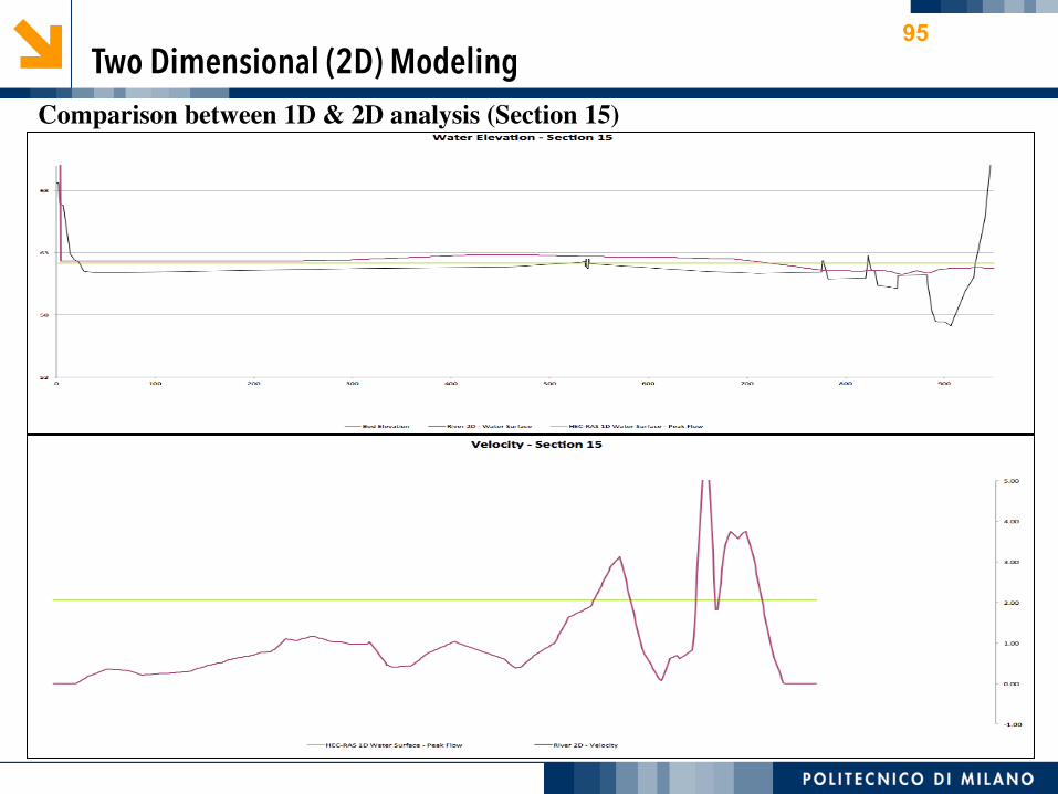
95 Two Dimensional (2D) Modeling
Comparison between 1D & 2D analysis (Section 15)

96 Two Dimensional (2D) Modeling
Comparison between 1D & 2D analysis (Section 16)

97 Two Dimensional (2D) Modeling
Comparison between 1D & 2D analysis (Section 17)
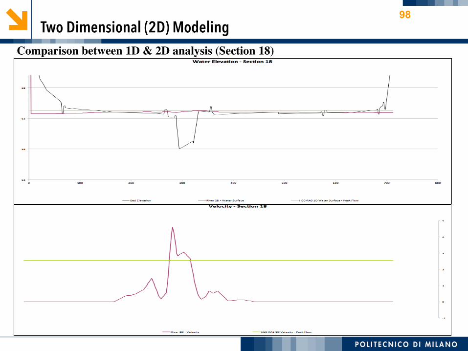
98 Two Dimensional (2D) Modeling
Comparison between 1D & 2D analysis (Section 18)

99 Two Dimensional (2D) Modeling
Comparison between 1D & 2D analysis (Section 20)

100 Two Dimensional (2D) Modeling
• General Comments �
Below is mentioned several reasons to explain the difference in the values of velocity obtained by 1D and 2D Software:
v ︎Hec-Ras considers only velocity for each section along the channel (so perpendicular to the cross sections), but River2D considers two components for velocity (in X direction and Y direction).
v In 2D modeling, lateral stresses are also considered while in the 1D modeling only friction losses are considered.
v ︎Therefore, there is only one values for velocity in 1D, however in 2D, velocity varies along the section and usually increase in main channel and decreases in flood plains.

101 Sediment Transport
Basic characteristic of the sediment
The value used :

102 Sediment Transport

103 Sediment Transport
m

104 Sediment Transport

105 Sediment Transport

106 Sediment Transport

107 Sediment Transport
Results:
² Where the value of τ* is greater than τ*critical we have bed load.
² As we can see in the previous graphs in the case of the peak flow in the
most of the sections we have bed load. But we have less sections with bed
loads in the ordinary case.

108 Sediment Transport

109 Sediment Transport

110 Sediment Transport

111 Sediment Transport
Conclusion :
Ø It is verified by the graphs that we have suspended load if the d50 is lower than ds critical (suspended)
Ø As demonstrated in the graphs we will have suspended
load in more sections in peak flow in comparison with ordinary flow.
Ø Occurring the bed load is more probable than the suspended load.

112 Sediment Transport
Ordinary flow :
Distance River Sta Q Total Froude # Chl Hydr Radius Channel Vel channel S (f,skin) τ0 τ* Critical τ*
14329 20 25 0.2 1.12 0.68 0.000176428 1.938453484 0.045 0.008233323
13860 19 25 1.02 0.41 2.07 0.006243145 25.1105546 0.045 0.106653732
13481 18 25 0.11 1.59 0.44 4.62967E-05 0.722131923 0.045 0.003067159
12945 17 25 0.26 1.07 0.85 0.000292977 3.075295304 0.045 0.013061907
12458 16 25 0.23 0.75 0.63 0.000258488 1.90182657 0.045 0.008077755
11385 15 25 0.4 0.84 1.14 0.000727688 5.996440197 0.045 0.02546908
10899 14 25 0.33 0.79 0.93 0.000525579 4.073181534 0.045 0.017300295
10503 13 25 0.12 1.19 0.41 5.91579E-05 0.690603793 0.045 0.002933248
9794 12 25 0.37 1.07 1.2 0.000583927 6.129308287 0.045 0.026033419
9219 11 25 0.19 1.19 0.65 0.000148687 1.735753138 0.045 0.00737238
8795 10 25 0.16 1.3 0.58 0.000105222 1.341894695 0.045 0.005699519
7893 9 25 0.35 0.62 0.86 0.000620844 3.776097843 0.045 0.016038472
6471 8 25 0.18 1.19 0.63 0.000139677 1.630580877 0.045 0.006925675
5490 7 25 0.21 1.07 0.67 0.000182031 1.910726729 0.045 0.008115557
4895 6.15 25 0.41 0.59 1 0.00089682 5.190703582 0.045 0.022046821
4875 6.05 25 1 0.37 1.93 0.006223292 22.58868467 0.045 0.095942426
4033 6 25 0.17 1.35 0.62 0.000114335 1.51419691 0.045 0.006431349
3532 5 25 0.17 1.2 0.57 0.00011307 1.331065812 0.045 0.005653525
2297 4 25 0.26 1.38 1.02 0.000300517 4.068342874 0.045 0.017279744
1501 3 25 0.3 0.93 0.93 0.000422827 3.857581827 0.045 0.016384564
1097 2.1 25 0.33 0.75 0.91 0.000539315 3.968008523 0.045 0.016853587
550 2 25 0.19 1.25 0.69 0.000156913 1.924147718 0.045 0.008172561
0 1 25 0.3 0.69 0.79 0.000454252 3.07478475 0.045 0.013059738
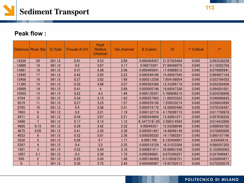
113 Sediment Transport
Peak flow :
Distance River Sta Q Total Froude # Chl Hydr
Radius Channel
Vel channel S (f,skin) τ0 τ* Critical τ*
14329 20 561.12 0.41 4.53 2.89 0.000494507 21.97555494 0.045 0.093338239
13860 19 561.12 0.5 3.87 3.17 0.00073397 27.86496075 0.045 0.118352704
13481 18 561.12 0.37 4.38 2.56 0.000405841 17.43808512 0.045 0.074065941
12945 17 561.12 0.42 2.85 2.23 0.000546166 15.26997545 0.045 0.064857184
12458 16 561.12 0.27 3.82 1.69 0.000212258 7.954188054 0.045 0.033784353
11385 15 561.12 0.35 3.46 2.07 0.000363368 12.33366716 0.045 0.052385606
10899 14 561.12 0.41 4 2.69 0.000505746 19.84547336 0.045 0.084291001
10503 13 561.12 0.22 4.3 1.46 0.000135287 5.706806219 0.045 0.024238898
9794 12 561.12 0.34 3.15 1.93 0.000357993 11.06253522 0.045 0.046986643
9219 11 561.12 0.27 3.23 1.57 0.000229106 7.259533219 0.045 0.030833899
8795 10 561.12 0.4 3.56 2.41 0.000474179 16.56002489 0.045 0.070336497
7893 9 561.12 0.2 3.21 1.19 0.000132718 4.179289715 0.045 0.017750976
6471 8 561.12 0.34 3.97 2.21 0.000344804 13.42861671 0.045 0.057036259
5490 7 561.12 0.17 4.15 1.12 8.34731E-05 3.398314584 0.045 0.014433888
4895 6.15 561.12 0.39 3.42 2.32 0.00046357 15.55288046 0.045 0.066058785
4875 6.05 561.12 0.41 3.35 2.38 0.000501497 16.48096149 0.045 0.070000686
4033 6 561.12 0.32 5.01 2.36 0.000288325 14.17060297 0.045 0.060187746
3532 5 561.12 0.26 4.7 1.77 0.0001766 8.142494607 0.045 0.03458416
2297 4 561.12 0.4 3.2 2.35 0.000519729 16.31533384 0.045 0.069297205
1501 3 561.12 0.52 3.54 3.18 0.000831811 28.88661936 0.045 0.122692063
1097 2.1 561.12 0.3 3.39 1.75 0.000266881 8.875369257 0.045 0.037696947
550 2 561.12 0.25 3.45 1.48 0.000186469 6.310938751 0.045 0.026804871
0 1 561.12 0.39 3.75 2.46 0.000460967 16.95782013 0.045 0.072026079

114 Sediment Transport
In this part we calculate sediment transport rate by following equations:

115 Sediment Transport
Calculating sediment transport (using different equation )

116 Sediment Transport

117 Sediment Transport

118 Sediment Transport
Result:
u As can be observe from the graphs the least sediment transport ratio is for Van Rijn equation and the highest sediment transport ratio correspond to Nielsen equation.
u However depending on qs morphological evolution of river bed will change river condition (manning coefficient, river geometry and so on)
u Considering the manning formula hf=10.29 n2 . D-5.33 . Q2 . L with respect to the sediment transport, the value of friction losses and roughness are changed. So for designing the channels for the long period of time the average manning coefficient is normally considered in the most cases.