Blind Source Camera Identification

Introduction

In today’s digital age, the creation and manipulation of digital images is

made simple by digital processing tools that are easily and widely

available. As a consequence, we can no longer take the authenticity of

images, analog or digital, for granted. This is especially true when it comes

to legal photographic evidence

Introduction

Although digital watermarks have been proposed as a tool to provide

authenticity to images, it is a fact that the overwhelming majority of

images that are captured today do not contain a digital watermark.

And this situation is likely to continue for the foreseeable future.

Problem Statement

There are images from unknown source with no or untraceable

watermark, but it is known to originate from either one of limited given

standard cameras , say x, y, z. It is needed to classify the images into

the groups based on originality. So the problem simplifies to whether a

particular image came was originated from camera x, camera y or

camera z.

Related Works

A number of features of images have been identified that can

prove to be a crucial part in classification .

Classification of the images have been a matter of study for past

few years and it has been done with maximum achieved average

accuracy of 93.42 % for set of two cameras, namely Nikon and

Sony.

Classification of images among 5 different cameras has been

conducted with an average accuracy of 88.02 %.

It is found out that a full generality of classification i.e. classification

among a set of unknown number of devices , is difficult on a higher

level.

Goals and Objectives

Identifying features that can be used in classification.

Develop a classifier function that classifies images into two groups

based on originality.

Methodology

34 features have been identified till now that are and can be used

in classification.

The features are mentioned in the following slides :-

AVERAGE PIXEL VALUE

This measure is based on the gray world assumption, which states

that the average values in RGB channels of an image should

average to gray, assuming that the images has enough color

variations. Thus the features are the mean value of the 3 RGB

channels (3 features).

RGB PAIRS CORRELATION

This measure attempts to capture the fact that depending

on the camera structure, the correlation between different color

bands could vary. There are 3 correlation pairs, namely RG, RB (3

features).

NEIGHBOR DISTRIBUTION CENTER OF MASS

This measure is calculated for each color band separately

by first calculating the number of pixel neighbors for each pixel

value, where a pixels neighbor are defined as all pixels which

have a difference of value of 1 or -1, from the pixel value in

question.

RGB pairs energy ratio

It is important because it is used in the process of white point correction which

is an integral part of a camera pipeline. The calculated features (3 features) are:

E1 = |G|2 /|B|2

E2 = |G|2 /|R|2

E3 = |B|2 /|R|2

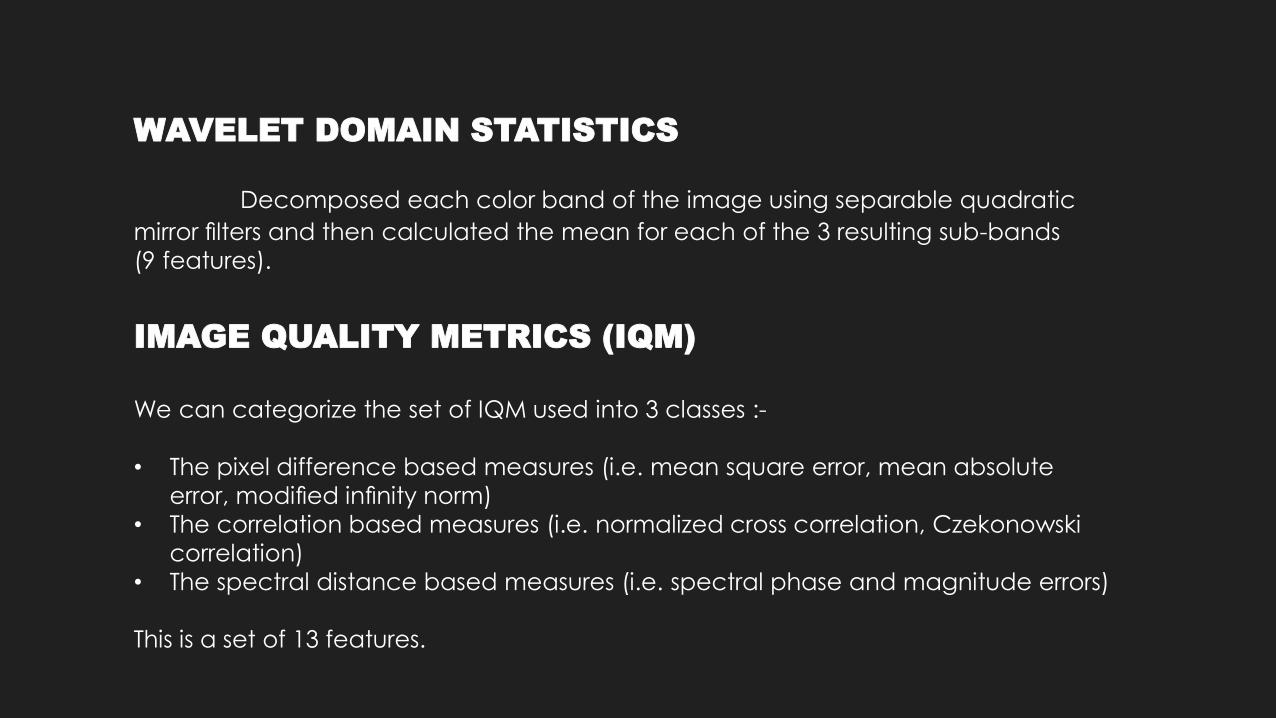
WAVELET DOMAIN STATISTICS

Decomposed each color band of the image using separable quadratic

mirror filters and then calculated the mean for each of the 3 resulting sub-bands

(9 features).

IMAGE QUALITY METRICS (IQM)

We can categorize the set of IQM used into 3 classes :-

• The pixel difference based measures (i.e. mean square error, mean absolute

error, modified infinity norm)

• The correlation based measures (i.e. normalized cross correlation, Czekonowski

correlation)

• The spectral distance based measures (i.e. spectral phase and magnitude errors)

This is a set of 13 features.

Classifier

• We are going to use Support Vector Machine(SVM) Classifier.

• It is primarily a classier method that performs classification tasks by

constructing hyper planes in a multidimensional space.

• To construct an optimal hyper plane, SVM employs an iterative

training algorithm, which is used to minimize an error function.

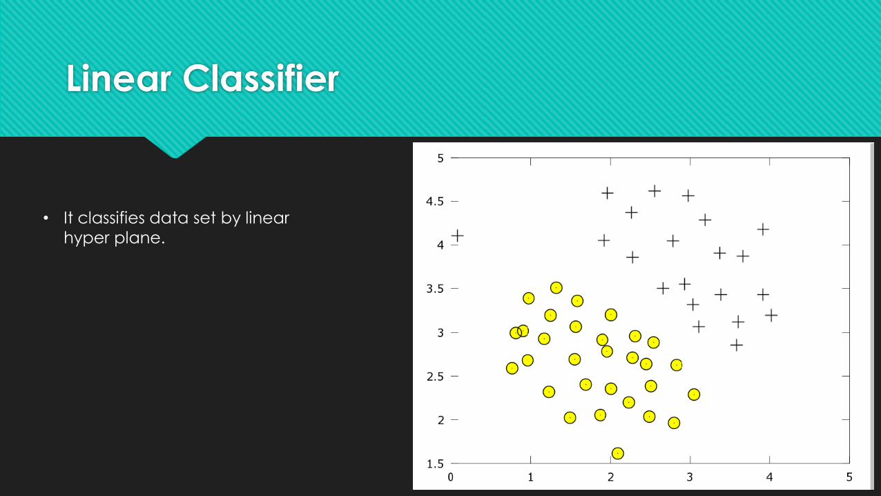
Linear Classifier

• It classifies data set by linear

hyper plane.

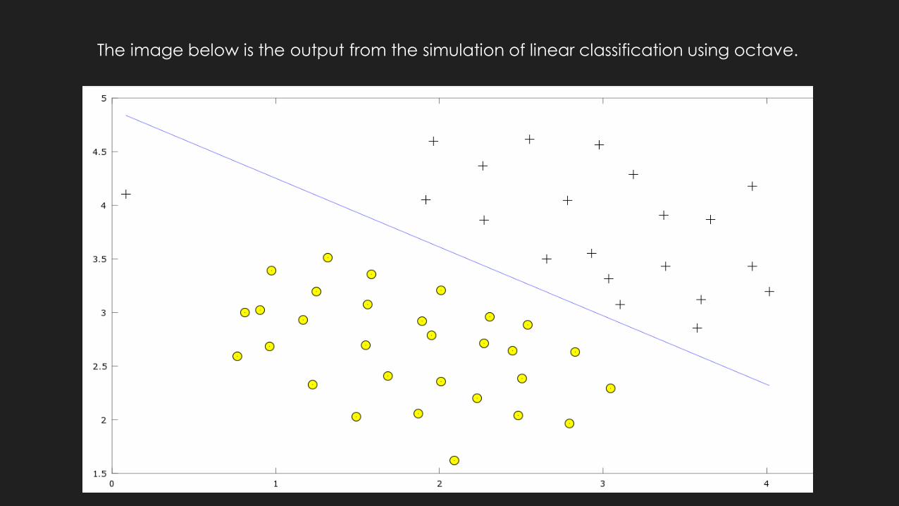
The image below is the output from the simulation of linear classification using octave.

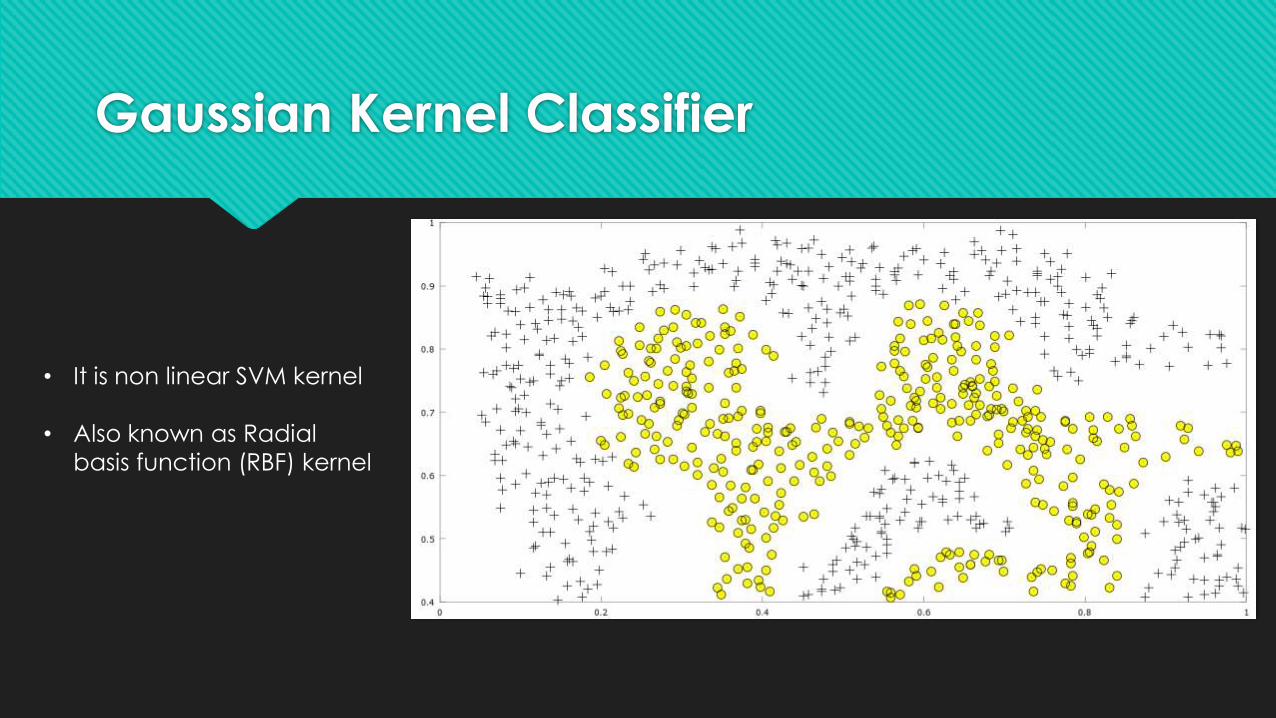
Gaussian Kernel Classifier

• It is non linear SVM kernel

• Also known as Radial

basis function (RBF) kernel

The image beside is the

output from the simulation

of Gaussian classification

using octave.

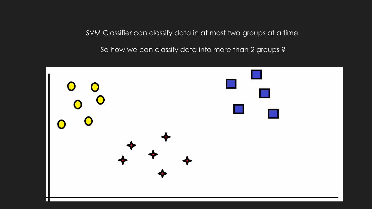
SVM Classifier can classify data in at most two groups at a time.

So how we can classify data into more than 2 groups ?

We can do that by training 3 classifiers , for each group vs all other groups

Group1 vs All

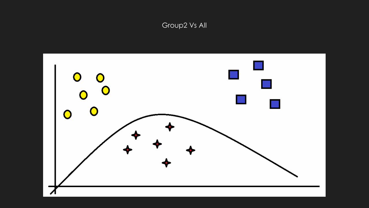
Group2 Vs All

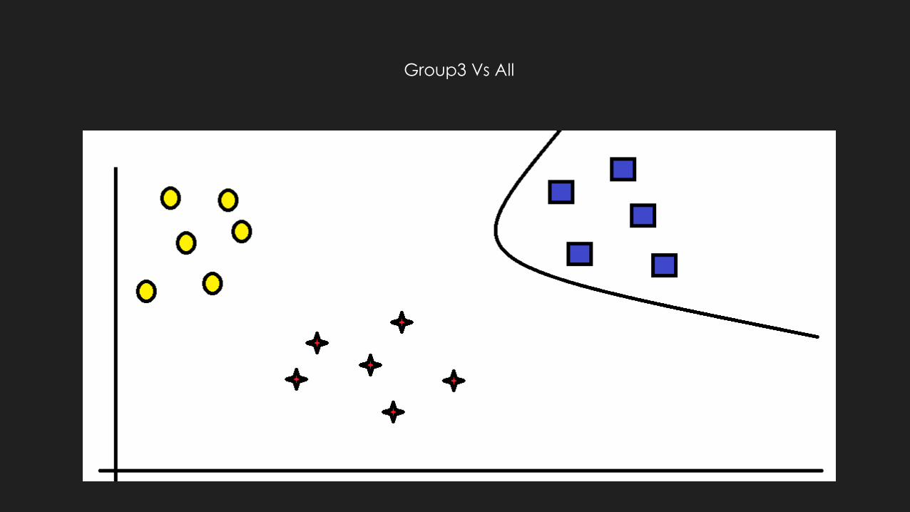
Group3 Vs All

Conclusion

The technique studied in the research project will

aide in improvement in performance and accuracy

of blind source camera identification.

Reference

[1] Mehdi Kharrazi , Husrev T. Sencar and Nasir Memon ,

”Blind Source Camera Identification”.

[2] C.-C. Chang and C.-J. Lin, LIBSVM: a library for support vector

machines, 2001, software available at

http://www.csie.ntu.edu.tw/˜cjlin/libsvm.

[3] Andrew Ng, ”Machine Learning CS-229 Standford”

http://cs229.standford.edu