Embed Size (px)
Citation preview

Data Structures and Algorithms
Algorithm: Outline, the essence of a computational procedure, step-by-step instructionsProgram: an implementation of an algorithm in some programming language Data structure: Organization of data needed to solve the problem

Algorithmic problem
Infinite number of input instances satisfying the specification. For eg: A sorted, non-decreasing sequence of natural numbers of non-zero, finite length:
1, 20, 908, 909, 100000, 1000000000.
3.
Specification of input
?Specification of output as a function of input

Algorithmic Solution
Algorithm describes actions on the input instanceInfinitely many correct algorithms for the same algorithmic problem
Input instance, adhering to the specification
Algorithm Output related to the input as required

What is a Good Algorithm?Efficient:
Running timeSpace used
Efficiency as a function of input size:The number of bits in an input number Number of data elements (numbers, points)

Measuring the Running Time
Experimental StudyWrite a program that implements the algorithmRun the program with data sets of varying size and composition.Use a method like System.currentTimeMillis() to get an accurate measure of the actual running time.
How should we measure the running time of an algorithm?

Limitations of Experimental Studies
It is necessary to implement and test the algorithm in order to determine its running time. Experiments can be done only on a limited set of inputs, and may not be indicative of the running time on other inputs not included in the experiment. In order to compare two algorithms, the same hardware and software environments should be used.

Beyond Experimental Studies
We will develop a general methodology for analyzing running time of algorithms. This approach
Uses a high-level description of the algorithm instead of testing one of its implementations. Takes into account all possible inputs. Allows one to evaluate the efficiency of any algorithm in a way that is independent of the hardware and software environment.

Pseudo-CodeA mixture of natural language and high-level programming concepts that describes the main ideas behind a generic implementation of a data structure or algorithm.Eg: Algorithm arrayMax(A, n):
Input: An array A storing n integers.Output: The maximum element in A.currentMax ← A[0]for i ← 1 to n-1 do
if currentMax < A[i] then currentMax ← A[i]return currentMax

Pseudo-Code It is more structured than usual prose butless formal than a programming language
Expressions: use standard mathematical symbols to describe numeric and boolean expressions use ← for assignment (“=” in Java)use = for the equality relationship (“==” in Java)
Method Declarations: Algorithm name(param1, param2)

Pseudo CodeProgramming Constructs:
decision structures: if ... then ... [else ... ] while-loops: while ... do repeat-loops: repeat ... until ...for-loop: for ... doarray indexing: A[i], A[i,j]
Methods:calls: object method(args)returns: return value

Analysis of Algorithms
Primitive Operation: Low-level operation independent of programming language. Can be identified in pseudo-code. For eg:
Data movement (assign)Control (branch, subroutine call, return)arithmetic an logical operations (e.g. addition, comparison)
By inspecting the pseudo-code, we can count the number of primitive operations executed by an algorithm.

Sort
Example: SortingINPUTsequence of numbers
a1, a2, a3,….,anb1,b2,b3,….,bn
OUTPUTa permutation of the sequence of numbers
2 5 4 10 7 2 4 5 7 10
Correctness (requirements for the output)For any given input the algorithm halts with the output:
• b1 < b2 < b3 < …. < bn• b1, b2, b3, …., bn is a permutation of a1, a2, a3,….,an
Running timeDepends on
• number of elements (n)• how (partially) sortedthey are
• algorithm

Insertion Sort
A1 nj
3 6 84 9 7 2 5 1
i
Strategy
• Start “empty handed”• Insert a card in the rightposition of the already sortedhand
• Continue until all cards areinserted/sorted
INPUT: A[1..n] – an array of integersOUTPUT: a permutation of A such that A[1]≤ A[2]≤ …≤A[n]
for j←2 to n dokey ← A[j]Insert A[j] into the sorted sequence A[1..j-1]i←j-1while i>0 and A[i]>key
do A[i+1]←A[i]i--
A[i+1]←key

Analysis of Insertion Sort
for j←2 to n dokey←A[j]Insert A[j] into the sorted sequence A[1..j-1]i←j-1while i>0 and A[i]>keydo A[i+1]←A[i]
i--A[i+1] ← key
costc1c20
c3c4c5c6c7
timesnn-1n-1
n-1
n-1
2
njj
t=∑
2( 1)n
jjt
=−∑
2( 1)n
jjt
=−∑
Total time = n(c1+c2+c3+c7) + ∑nj=2 tj (c4+c5+c6)
– (c2+c3+c5+c6+c7)

Best/Worst/Average Case
Best case: elements already sorted; tj=1, running time = f(n), i.e., linear time. Worst case: elements are sorted in inverse order; tj=j, running time = f(n2), i.e.,quadratic timeAverage case: tj=j/2, running time = f(n2),i.e., quadratic time
Total time = n(c1+c2+c3+c7) + ∑nj=2 tj (c4+c5+c6)
– (c2+c3+c5+c6+c7)

Best/Worst/Average Case (2)
For a specific size of input n, investigate running times for different input instances:

Best/Worst/Average Case (3)For inputs of all sizes:
1n
2n
3n
4n
5n
6n
Input instance size
Run
ning
tim
e
1 2 3 4 5 6 7 8 9 10 11 12 …..
best-case
average-case
worst-case
Best/Worst/Average Case (4)
Worst case is usually used: It is an upper-bound and in certain application domains (e.g., air traffic control, surgery) knowing the worst-case time complexity is of crucial importanceFor some algorithms worst case occurs fairly oftenAverage case is often as bad as the worst caseFinding average case can be very difficult
Asymptotic AnalysisGoal: to simplify analysis of running time by getting rid of ”details”, which may be affected by specific implementation and hardware
like “rounding”: 1,000,001 ≈ 1,000,0003n2 ≈ n2
Capturing the essence: how the running time of an algorithm increases with the size of the input in the limit.
Asymptotically more efficient algorithms are best for all but small inputs

Asymptotic NotationThe “big-Oh” O-Notation
asymptotic upper boundf(n) is O(g(n)), if there exists constants c and n0, s.t. f(n) ≤ c g(n) for n≥ n0f(n) and g(n) are functions over non-negative integers
Used for worst-caseanalysis
)(nf( )c g n⋅
0n Input Size
Run
ning
Tim
e

ExampleFor functions f(n) and g(n) there are positive constants c and n0 such that: f(n) ≤ c g(n) for n ≥ n0
conclusion:
2n+6 is O(n).

Another Example
On the other hand…n2 is not O(n) because there is no c and n0 such that:
n2 ≤ cn for n ≥ n0
The graph to the right illustrates that no matter how large a c is chosen there is an n big enough that n2 > cn ) .

Asymptotic NotationSimple Rule: Drop lower order terms and constant factors.
50 n log n is O(n log n)7n - 3 is O(n)8n2 log n + 5n2 + n is O(n2 log n)
Note: Even though (50 n log n) is O(n5), it is expected that such an approximation be of as small an order as possible
Asymptotic Analysis of Running TimeUse O-notation to express number of primitive operations executed as function of input size.Comparing asymptotic running times
an algorithm that runs in O(n) time is better than one that runs in O(n2) timesimilarly, O(log n) is better than O(n)hierarchy of functions: log n < n < n2 < n3 < 2n
Caution! Beware of very large constant factors. An algorithm running in time 1,000,000 n is still O(n) but might be less efficient than one running in time 2n2, which is O(n2)

Example of Asymptotic AnalysisAlgorithm prefixAverages1(X):Input: An n-element array X of numbers.Output: An n-element array A of numbers such that
A[i] is the average of elements X[0], ... , X[i].for i ← 0 to n-1 do
a ← 0for j ← 0 to i do
a ← a + X[j] A[i] ← a/(i+1)
return array AAnalysis: running time is O(n2)
1 step
i iterations with i=0,1,2...n-1
n iterations

A Better AlgorithmAlgorithm prefixAverages2(X):Input: An n-element array X of numbers.Output: An n-element array A of numbers suchthat A[i] is the average of elements X[0], ... , X[i].s ← 0for i ← 0 to n do
s ← s + X[i] A[i] ← s/(i+1)
return array AAnalysis: Running time is O(n)

Asymptotic Notation (terminology)
Special classes of algorithms:Logarithmic: O(log n)Linear: O(n)Quadratic: O(n2)Polynomial: O(nk), k ≥ 1Exponential: O(an), a > 1
“Relatives” of the Big-OhΩ (f(n)): Big Omega -asymptotic lower boundΘ (f(n)): Big Theta -asymptotic tight bound

The “big-Omega” Ω−Notation
asymptotic lower boundf(n) is Ω(g(n)) if there exists constants c and n0, s.t. c g(n) ≤ f(n) for n ≥ n0
Used to describe best-case running times or lower bounds for algorithmic problems
E.g., lower-bound for searching in an unsorted array is Ω(n).
Input Size
Run
ning
Tim
e )(nf( )c g n⋅
0n
Asymptotic Notation

The “big-Theta” Θ−Notationasymptotically tight boundf(n) = Θ(g(n)) if there exists constants c1, c2, and n0, s.t. c1 g(n) ≤ f(n) ≤ c2 g(n) for n ≥n0
f(n) is Θ(g(n)) if and only if f(n) is Ο(g(n)) and f(n) is Ω(g(n))O(f(n)) is often misused instead of Θ(f(n))
Asymptotic Notation
Input SizeR
unni
ng T
ime )(nf
0n
)(ngc ⋅2
)(ngc ⋅1

Asymptotic NotationTwo more asymptotic notations
"Little-Oh" notation f(n) is o(g(n))non-tight analogue of Big-Oh
For every c, there should exist n0 , s.t. f(n) ≤ c g(n) for n ≥ n0
Used for comparisons of running times. If f(n)=o(g(n)), it is said that g(n) dominates f(n).
"Little-omega" notation f(n) is ω(g(n))non-tight analogue of Big-Omega

Asymptotic NotationAnalogy with real numbers
f(n) = O(g(n)) ≅ f ≤ gf(n) = Ω(g(n)) ≅ f ≥ gf(n) = Θ(g(n)) ≅ f = gf(n) = o(g(n)) ≅ f < gf(n) = ω(g(n)) ≅ f > g
Abuse of notation: f(n) = O(g(n)) actually means f(n) ∈O(g(n))

Comparison of Running Times
RunningTime
Maximum problem size (n)
1 second 1 minute 1 hour
400n 2500 150000 9000000
20n log n 4096 166666 7826087
2n2 707 5477 42426
n4 31 88 244
2n 19 25 31

Correctness of AlgorithmsThe algorithm is correct if for any legal input it terminates and produces the desired output.Automatic proof of correctness is not possibleBut there are practical techniques and rigorous formalisms that help to reason about the correctness of algorithms

Partial and Total Correctness
Partial correctness
Any legal input Algorithm Output
IF this point is reached, THEN this is the desired output
Total correctness
Any legal input Algorithm Output
INDEED this point is reached, AND this is the desired output

AssertionsTo prove correctness we associate a number of assertions (statements about the state of the execution) with specific checkpoints in the algorithm.
E.g., A[1], …, A[k] form an increasing sequencePreconditions – assertions that must be valid before the execution of an algorithm or a subroutinePostconditions – assertions that must be valid after the execution of an algorithm or a subroutine

Loop InvariantsInvariants – assertions that are valid any time they are reached (many times during the execution of an algorithm, e.g., in loops)We must show three things about loop invariants:
Initialization – it is true prior to the first iterationMaintenance – if it is true before an iteration, it remains true before the next iterationTermination – when loop terminates the invariant gives a useful property to show the correctness of the algorithm
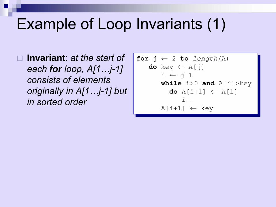
Example of Loop Invariants (1)
Invariant: at the start of each for loop, A[1…j-1] consists of elements originally in A[1…j-1] but in sorted order
for j ← 2 to length(A)do key ← A[j]
i ← j-1while i>0 and A[i]>keydo A[i+1] ← A[i]
i--A[i+1] ← key
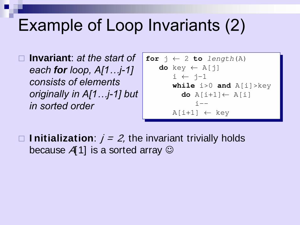
Example of Loop Invariants (2)
Invariant: at the start of each for loop, A[1…j-1] consists of elements originally in A[1…j-1] but in sorted order
for j ← 2 to length(A)do key ← A[j]
i ← j-1while i>0 and A[i]>keydo A[i+1]← A[i]
i--A[i+1] ← key
Initialization: j = 2, the invariant trivially holds because A[1] is a sorted array ☺

Example of Loop Invariants (3)
Invariant: at the start of each for loop, A[1…j-1] consists of elements originally in A[1…j-1] but in sorted order
for j ← 2 to length(A)do key ← A[j]
i ← j-1while i>0 and A[i]>keydo A[i+1] ← A[i]
i--A[i+1] ← key
Maintenance: the inner while loop moves elements A[j-1], A[j-2], …, A[j-k] one position right without changing their order. Then the former A[j] element is inserted into k-th position so that A[k-1] ≤ A[k] ≤A[k+1].
A[1…j-1] sorted + A[j] → A[1…j] sorted

Example of Loop Invariants (4)
Invariant: at the start of each for loop, A[1…j-1] consists of elements originally in A[1…j-1] but in sorted order
for j ← 2 to length(A)do key ← A[j]
i ← j-1while i>0 and A[i]>keydo A[i+1] ← A[i]
i--A[i+1] ← key
Termination: the loop terminates, when j=n+1. Then the invariant states: “A[1…n] consists of elements originally in A[1…n] but in sorted order” ☺

Math You Need to Review
Properties of logarithms:logb(xy) = logbx + logbylogb(x/y) = logbx - logbylogb xa = a logb xlogb a = logxa/logxb
Properties of exponentials:a(b+c) = abac ; abc = (ab)c
ab /ac = a(b-c) ; b = aloga b
Floor: ⎣x⎦ = the largest integer ≤ xCeiling: ⎡x⎤ = the smallest integer ≥ x
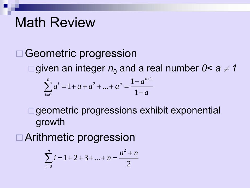
Math Review
Geometric progressiongiven an integer n0 and a real number 0< a ≠ 1
geometric progressions exhibit exponential growth
Arithmetic progression
12
0
11 ...1
nni n
i
aa a a aa
+
=
−= + + + + =
−∑
2
01 2 3 ...
2
n
i
n ni n=
+= + + + + =∑

SummationsThe running time of insertion sort is determined by a nested loop
Nested loops correspond to summations
for j←2 to length(A)key←A[j]i←j-1while i>0 and A[i]>key
A[i+1]←A[i]i←i-1
A[i+1]←key
22( 1) ( )n
jj O n
=− =∑

Proof by InductionWe want to show that property P is true for all integers n ≥ n0
Basis: prove that P is true for n0
Inductive step: prove that if P is true for all k such that n0 ≤ k ≤ n – 1 then P is also true for nExample
Basis
0
( 1)( ) for 12
n
i
n nS n i n=
+= = ≥∑
1
0
1(1 1)(1)2i
S i=
+= =∑

Proof by Induction (2)
0
1
0 02
( 1)( ) for 1 k 12
( ) ( 1)
( 1 1) ( 2 )( 1)2 2
( 1)2
k
i
n n
i i
k kS k i n
S n i i n S n n
n n n nn n
n n
=
−
= =
+= = ≤ ≤ −
= = + = − + =
− + − += − + = =
+=
∑
∑ ∑
Inductive Step