Characterization of the Wireless Channel

Ch.2. Characterization of the Wireless Channel

2.1 Multipath Propagation

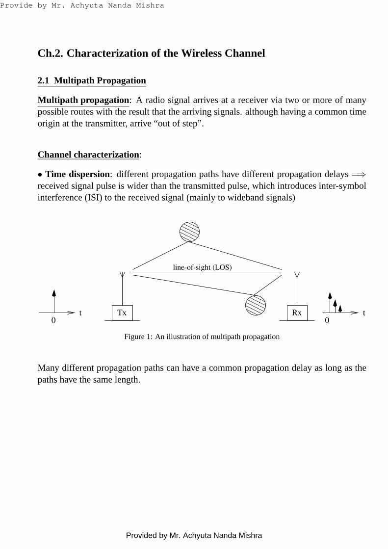
Multipath propagation : A radio signal arrives at a receiver via two or more of manypossible routes with the result that the arriving signals. although having a common timeorigin at the transmitter, arrive “out of step”.

Channel characterization:

• Time dispersion: different propagation paths have different propagation delays=⇒received signal pulse is wider than the transmitted pulse, which introduces inter-symbolinterference (ISI) to the received signal (mainly to wideband signals)

Tx0

t

line-of-sight (LOS)

Rx t0

Figure 1: An illustration of multipath propagation

Many different propagation paths can have a common propagation delay as long as thepaths have the same length.

Provide by Mr. Achyuta Nanda Mishra

Provided by Mr. Achyuta Nanda Mishra

Wireless Communications and Networking Ch2 - Page 2 of 44

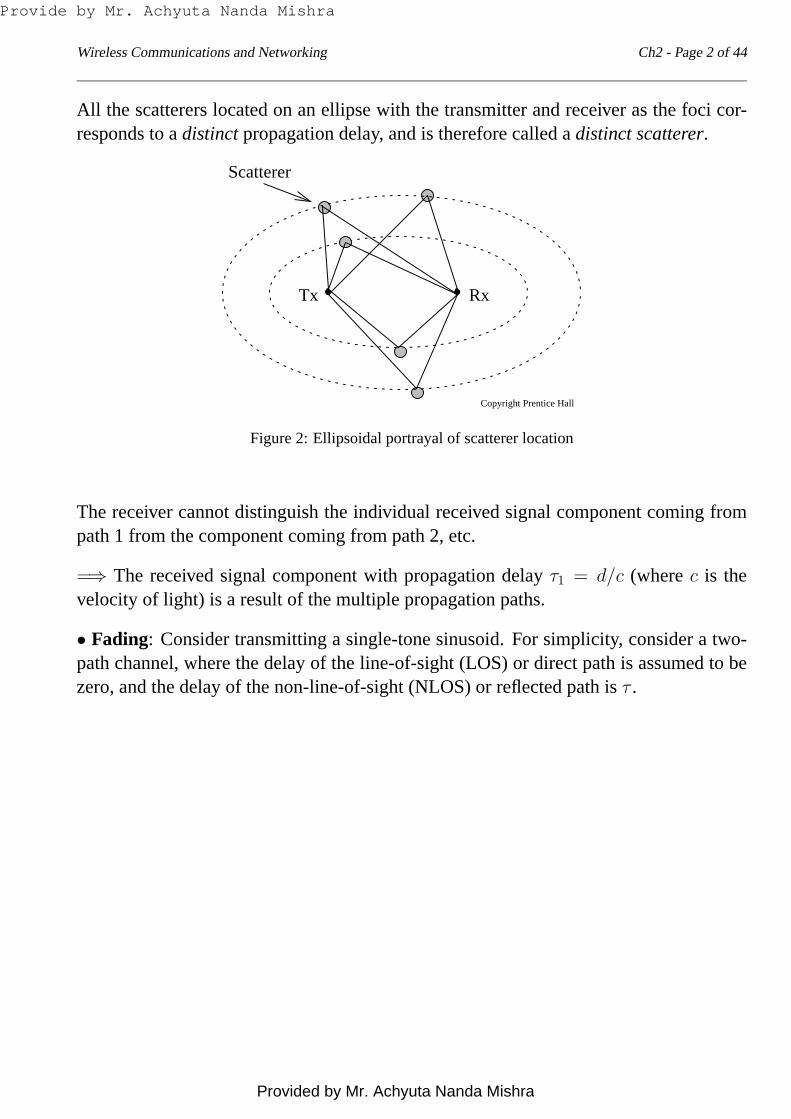
All the scatterers located on an ellipse with the transmitter and receiver as the foci cor-responds to adistinct propagation delay, and is therefore called adistinct scatterer.

Copyright Prentice Hall

Scatterer

RxTx

Figure 2: Ellipsoidal portrayal of scatterer location

The receiver cannot distinguish the individual received signal component coming frompath 1 from the component coming from path 2, etc.

=⇒ The received signal component with propagation delayτ1 = d/c (wherec is thevelocity of light) is a result of the multiple propagation paths.

• Fading: Consider transmitting a single-tone sinusoid. For simplicity, consider a two-path channel, where the delay of the line-of-sight (LOS) or direct path is assumedto bezero, and the delay of the non-line-of-sight (NLOS) or reflected path isτ .




Transmitter

Receiver

c© Prentice Hall

α1 cos(2πfct)

α2 cos(2πfc(t − τ))

Figure 3: A channel with two propagation paths

The received signal, in the absence of noise, can be represented as

r(t) = α1 cos(2πfct) + α2 cos(2πfc(t − τ)), (1)

whereα1 andα2 are the amplitudes of the signal components from the two paths respec-tively. The received signal can also be represented as

r(t) = α cos(2πfct + φ), (2)

whereα =

√

α21 + α2

2 + 2α1α2 cos(2πfcτ)

and

φ = − tan−1[α2 sin(2πfcτ)

α1 + α2 cos(2πfcτ)]

are the amplitude and phase of the received signal. Bothα andφ are functions ofα1, α2,andτ .




0 0.5 1 1.5 2 2.50

0.5

1

1.5

2

2.5

3

3.5

4

fcτ

α1+α

2

α1−α

2

Prentice Hall

The

rec

eive

d si

gnal

am

plitu

de α

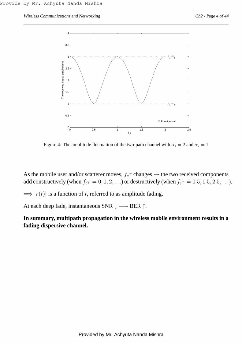
Figure 4: The amplitude fluctuation of the two-path channel with α1 = 2 andα2 = 1

As the mobile user and/or scatterer moves,fcτ changes→ the two received componentsadd constructively (whenfcτ = 0, 1, 2, . . .) or destructively (whenfcτ = 0.5, 1.5, 2.5, . . .).

=⇒ |r(t)| is a function oft, referred to as amplitude fading.

At each deep fade, instantaneous SNR↓ −→ BER↑.

In summary, multipath propagation in the wireless mobile environment results in afading dispersive channel.




2.2 The Linear Time-Variant Channel Model

Consider a multipath propagation environment withN distinct scatterers, each charac-terized by amplitude fluctuationαn(t) and propagation delayτn(t) , n = 1, 2, . . . , N .

Consider a narrowband signalx(t) transmitted over the wireless channel at a carrierfrequencyfc, such that

x(t) = ℜx(t)ej2πfct, (3)

wherex(t) is the complex envelope of the signal.

In the absence of background noise, the received signal at the channel output is

r(t) = ℜN∑

n=1

αn(t)x(t − τn(t))ej2πfc(t−τn(t))

= ℜr(t)ej2πfct,

wherer(t) is the complex envelope of the received signal and can be represented as

r(t) =N∑

n=1

αn(t)e−j2πfcτn(t)x(t − τn(t)). (4)

As the mobile user moves,αn(t) andτn(t) are a function oft =⇒ the channel is lineartime-variant.

=⇒ The channel impulse response depends on the instant that the impulse is applied tothe channel.




Channel impulse response

Linear time-invariant (LTI) channel:

00

0 0LTI channel

c© Prentice Hall

δ(t)

δ(t − t1)

t1

r(t) = h(t)

r(t) = h(t − t1)h(t)

x(t) r(t)

t

t

t

t

Figure 5: The linear time-invariant channel model

We can useh(t) to describe the channel, wheret is a variable describing propagationdelay, assuming that the impulse is always applied to the channel at time zero.

Linear time-variant (LTV) channel:

00

LTV channel 00

c© Prentice Hall

δ(t)

δ(t − t1)

t1

x(t) r(t)

h(τ, t)

r(t) = h1(t)

r(t) = h2(t) 6= h1(t − t1)

t

t

t

t

Figure 6: The linear time-variant channel model

The channel impulse response is a function of two variables: one describing when theimpulse is applied to the channel, the other describing the moment of observing thechannel output or the associated propagation delay.




Definition:

The impulse response of an LTV channel,h(τ, t), is the channel output att inresponse to an impulse applied to the channel att − τ .

The received signal is

r(t) =

∫ ∞

−∞h(τ, t)x(t − τ)dτ. (5)

The channel impulse response for the channel withN distinct scatterers is then

h(τ, t) =N∑

n=1

αn(t)e−jθn(t)δ(τ − τn(t)), (6)

whereθn(t) = 2πfcτn(t) represents the carrier phase distortion introduced by thenthscatterer.

Note:τn(t) changes by1/fc −→ θn(t) changes by2π=⇒ a small change in the propagation delay−→ a small change inαn(t) andτn(t), buta significant change inθn(t)

That is, the carrier phase distortionθn(t) is much more sensitive to user mobility thanthe amplitude fluctuationαn(t).




Time-variant transfer function

Linear time-invariant channel:

H(f) = F [h(t)] (7)

The channel output in the frequency domain is

R(f) = H(f)X(f). (8)

Linear time-variant channel:

Definition

The time-variant transfer function of an LTV channel is the Fourier transformof the impulse response,h(τ, t), with respect to the delay variableτ .

H(f, t) = Fτ [h(τ, t)] =∫ ∞−∞ h(τ, t)e−j2πfτdτ

h(τ, t) = F−1f [H(f, t)] =

∫ ∞−∞ H(f, t)e+j2πfτdf

where the time variablet can be viewed as a parameter.





r(t) =

∫ ∞

−∞h(τ, t)x(t − τ)dτ

=

∫ ∞

−∞x(t − τ)[

∫ ∞

−∞H(f, t) exp(j2πfτ)df ]dτ

=

∫ ∞

−∞H(f, t)

∫ ∞

−∞x(t − τ) exp[−j2πf(t − τ)]dτ exp(j2πft)df

=

∫ ∞

−∞H(f, t)[

∫ −∞

∞x(ξ) exp(−j2πfξ)(−dξ)] exp(j2πft)df

=

∫ ∞

−∞H(f, t)X(f) exp(j2πft)df

=

∫ ∞

−∞R(f, t) exp(j2πft)df

whereR(f, t) = H(f, t)X(f)

andX(f) = F [x(t)].




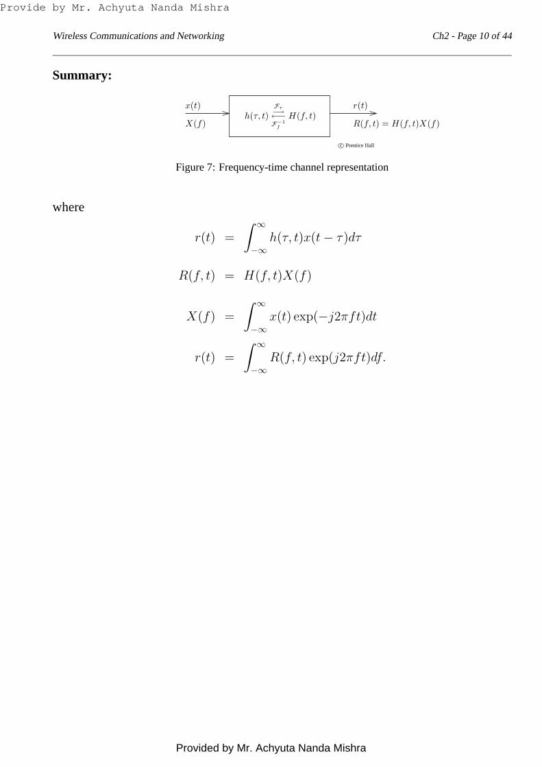
Summary:

c© Prentice Hall

x(t) r(t)

R(f, t) = H(f, t)X(f)X(f)h(τ, t)

Fτ−→←−F

−1

f

H(f, t)

Figure 7: Frequency-time channel representation

where

r(t) =

∫ ∞


R(f, t) = H(f, t)X(f)

X(f) =

∫ ∞

−∞x(t) exp(−j2πft)dt

r(t) =

∫ ∞

−∞R(f, t) exp(j2πft)df.




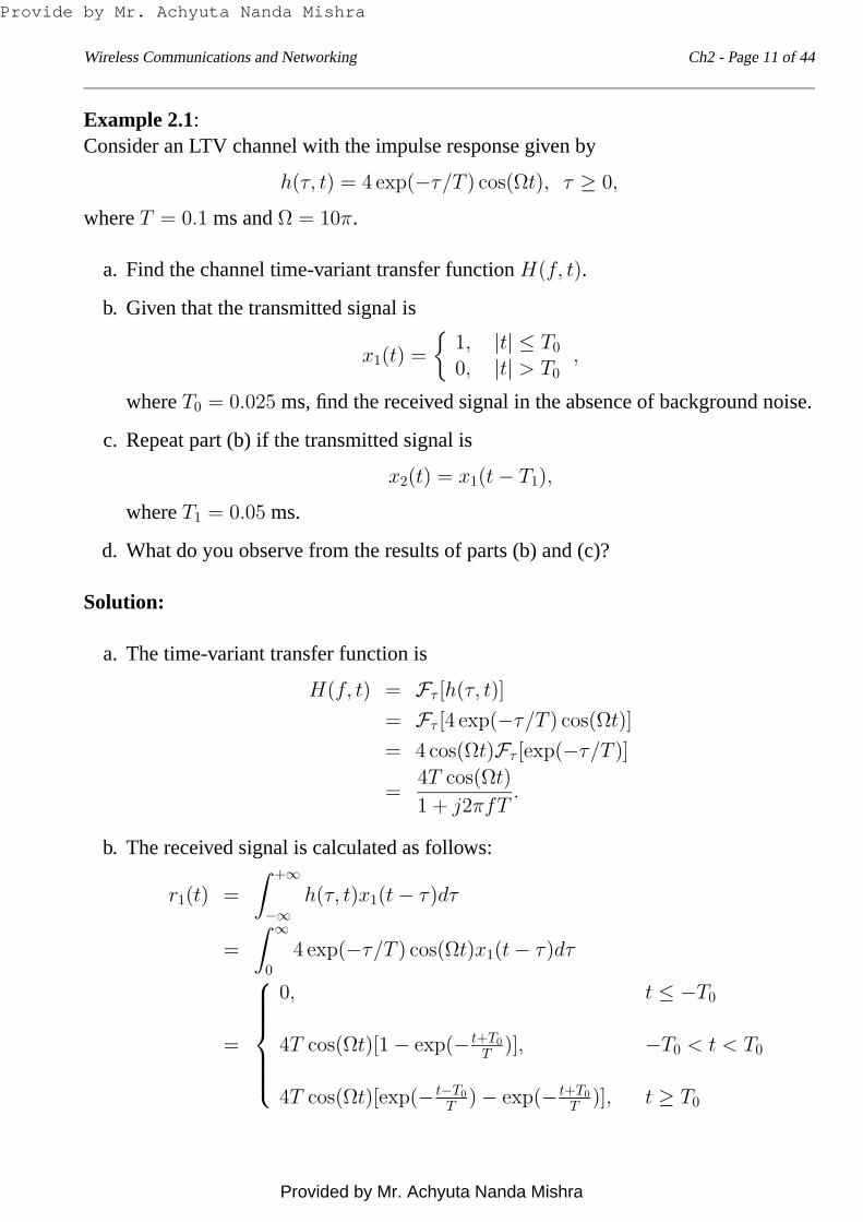
Example 2.1:Consider an LTV channel with the impulse response given by

h(τ, t) = 4 exp(−τ/T ) cos(Ωt), τ ≥ 0,

whereT = 0.1 ms andΩ = 10π.

a. Find the channel time-variant transfer functionH(f, t).

b. Given that the transmitted signal is

x1(t) =

1, |t| ≤ T0

0, |t| > T0,

whereT0 = 0.025 ms, find the received signal in the absence of background noise.

c. Repeat part (b) if the transmitted signal is

x2(t) = x1(t − T1),

whereT1 = 0.05 ms.

d. What do you observe from the results of parts (b) and (c)?

Solution:

a. The time-variant transfer function is

H(f, t) = Fτ [h(τ, t)]

= Fτ [4 exp(−τ/T ) cos(Ωt)]

= 4 cos(Ωt)Fτ [exp(−τ/T )]

=4T cos(Ωt)

1 + j2πfT.

b. The received signal is calculated as follows:

r1(t) =

∫ +∞

−∞h(τ, t)x1(t − τ)dτ

=

∫ ∞

0

4 exp(−τ/T ) cos(Ωt)x1(t − τ)dτ

=

0, t ≤ −T0

4T cos(Ωt)[1 − exp(− t+T0

T )], −T0 < t < T0

4T cos(Ωt)[exp(− t−T0

T ) − exp(− t+T0

T )], t ≥ T0




−0.1 −0.05 0 0.05 0.1 0.15 0.2 0.25 0.3 0.35 0.4−1.5

−1

−0.5

0

0.5

1

1.5

t (ms)

x 1(t)

and

r 1(t)

/ T

Prentice Hall

x1(t)

r1(t) / T

(a)

0 0.1 0.2 0.3 0.4 0.5−1.5

−1

−0.5

0

0.5

1

1.5

t (ms)

x 2(t)

and

r 2(t)

/ T

Prentice Hall

x2(t)

r2(t) / T

(b)

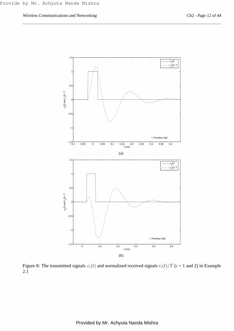
Figure 8: The transmitted signalsxi(t) and normalized received signalsri(t)/T (i = 1 and 2) in Example2.1




The transmitted and received signals are plotted in Figure 8(a).

c. Similar to part (b), the received signal is calculated as follows:

r2(t) =

∫ +∞

−∞h(τ, t)x2(t − τ)dτ

=

∫ ∞

0

4 exp(−τ/T ) cos(Ωt)x1(t − T1 − τ)dτ

=

0, t ≤ T1 − T0

4T cos(Ωt)[1 − exp(− t−T1+T0

T )], T1 − T0 < t < T1 + T0

4T cos(Ωt)[exp(− t−T1−T0

T ) − exp(− t−T1+T0

T )], t ≥ T1 + T0

The transmitted and received signals are plotted in Figure 8(b).

d. From Figure 8, it is observed that: (1) the received signals have a larger pulse widththan the corresponding transmitted signals because the channel is time dispersive;and (2) even though the transmitted signalx2(t) is x1(t) delayed byT1, the receivedsignalr2(t) is notr1(t) delayed byT1 because the channel is time varying.

¤




2.3 Channel Correlation Functions

Assumptions:

(a) the channel impulse responseh(τ, t) is a wide-sense stationary (WSS) process;

(b) the channel impulse responses atτ1 andτ2, h(τ1, t) andh(τ2, t), are uncorrelated ifτ1 6= τ2 for anyt.

→ wide-sense stationary uncorrelated scattering (WSSUS) channel

Delay power spectral density (psd)

The autocorrelation function ofh(τ, t) is

φh(τ1, τ2, ∆t)=

1

2E[h∗(τ1, t)h(τ2, t + ∆t)]

= φh(τ1, ∆t)δ(τ1 − τ2)

or equivalently,φh(τ, τ + ∆τ, ∆t) = φh(τ, ∆t)δ(∆τ), (9)

where

φh(τ, ∆t) =

∫

φh(τ, τ + ∆τ, ∆t)d∆τ.

At ∆t = 0, we define

φh(τ)= φh(τ, 0). (10)

From Eqs. (9) – (10), we have

φh(τ) = F∆τ [φh(τ, τ + ∆τ, ∆t)]|∆t=0

= F∆τ1

2E[h∗(τ, t)h(τ + ∆τ, t)].




φh(τ) measures the average psd at the channel output as a function of the propagationdelay,τ , and is therefore called the delay psd of the channel, also known as the multipathintensity profile. The nominal width of the delay psd pulse is called the multipath delayspread, denoted byTm.

0 c© Prentice Hall

φh(τ)

Tm

τ

Figure 9: Delay power spectral density

Thenth moment of the delays

τn =

∫τnφh(τ)dτ

∫φh(τ)dτ

. (11)

The mean propagation delay, or first moment, denoted byτ , is

τ =

∫τφh(τ)dτ

∫φh(τ)dτ

(12)

and the rms (root-mean-square) delay spread, denoted byστ , is

στ =

[∫(τ − τ)2φh(τ)dτ

∫φh(τ)dτ

]1/2

. (13)

In calculating a value for the multipath delay spread, it is usually assumedthat

Tm ≈ στ .




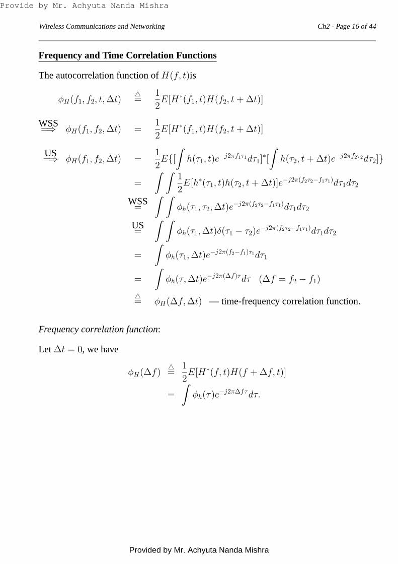
Frequency and Time Correlation Functions

The autocorrelation function ofH(f, t)is

φH(f1, f2, t, ∆t)=

1

2E[H∗(f1, t)H(f2, t + ∆t)]

WSS=⇒ φH(f1, f2, ∆t) =

1

2E[H∗(f1, t)H(f2, t + ∆t)]

US=⇒ φH(f1, f2, ∆t) =

1

2E[

∫

h(τ1, t)e−j2πf1τ1dτ1]

∗[

∫

h(τ2, t + ∆t)e−j2πf2τ2dτ2]

=

∫ ∫1

2E[h∗(τ1, t)h(τ2, t + ∆t)]e−j2π(f2τ2−f1τ1)dτ1dτ2

WSS=

∫ ∫

φh(τ1, τ2, ∆t)e−j2π(f2τ2−f1τ1)dτ1dτ2

US=

∫ ∫

φh(τ1, ∆t)δ(τ1 − τ2)e−j2π(f2τ2−f1τ1)dτ1dτ2

=

∫

φh(τ1, ∆t)e−j2π(f2−f1)τ1dτ1

=

∫

φh(τ, ∆t)e−j2π(∆f)τdτ (∆f = f2 − f1)

= φH(∆f, ∆t) — time-frequency correlation function.

Frequency correlation function:

Let ∆t = 0, we have

φH(∆f)=

1

2E[H∗(f, t)H(f + ∆f, t)]

=

∫

φh(τ)e−j2π∆fτdτ.




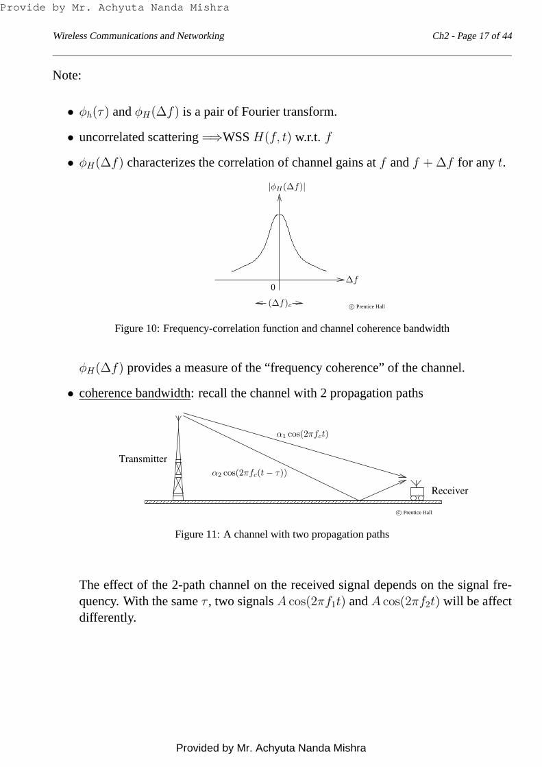
Note:

• φh(τ) andφH(∆f) is a pair of Fourier transform.

• uncorrelated scattering=⇒WSSH(f, t) w.r.t. f

• φH(∆f) characterizes the correlation of channel gains atf andf + ∆f for anyt.

0

c© Prentice Hall(∆f)c

∆f

|φH(∆f)|

Figure 10: Frequency-correlation function and channel coherence bandwidth

φH(∆f) provides a measure of the “frequency coherence” of the channel.

• coherence bandwidth: recall the channel with 2 propagation paths

Transmitter

Receiver

c© Prentice Hall

α1 cos(2πfct)

α2 cos(2πfc(t − τ))

Figure 11: A channel with two propagation paths

The effect of the 2-path channel on the received signal depends on the signal fre-quency. With the sameτ , two signalsA cos(2πf1t) andA cos(2πf2t) will be affectdifferently.




0 0.5 1 1.5 2 2.50

0.5

1

1.5

2

2.5

3

3.5

4

fcτ

α1+α

2

α1−α

2

Prentice Hall

The

rec

eive

d si

gnal

am

plitu

de α

Figure 12: The amplitude fluctuation of the two-path channelwith α1 = 2 andα2 = 1

=⇒ |f1 − f2| ↑ =⇒ |r1(t)| and|r2(t)| at anyt will be uncorrelated.

Definition: The maximum frequency difference for which the signals are still stronglycorrelated is called the coherence bandwidth of the channel, denoted by(∆f)c.

=⇒ Two sinusoids with frequency separation larger than(∆f)c are affected differ-ently by the channel at anyt.




• Let Ws denote the bandwidth of the transmitted signal.

If (∆f)c < Ws, the channel is said to exhibit frequency selective fading whichintroduces severe ISI to the received signal;

If (∆f)c ≫ Ws, the channel is said to exhibit frequency nonselective fading orflat fading which introduces negligible ISI.

• φh(τ) ↔ φH(∆f) =⇒ (∆f)c ≈ 1/Tm.




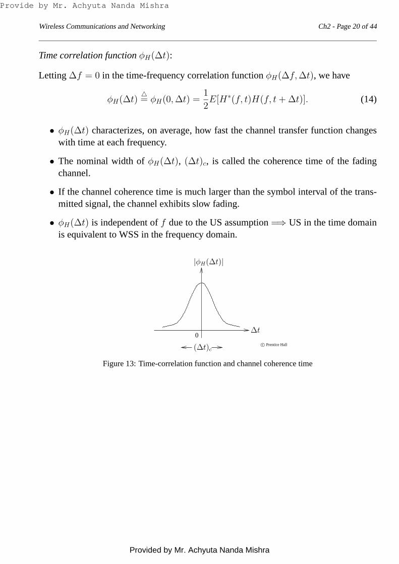
Time correlation function φH(∆t):

Letting∆f = 0 in the time-frequency correlation functionφH(∆f, ∆t), we have

φH(∆t)= φH(0, ∆t) =

1

2E[H∗(f, t)H(f, t + ∆t)]. (14)

• φH(∆t) characterizes, on average, how fast the channel transfer function changeswith time at each frequency.

• The nominal width ofφH(∆t), (∆t)c, is called the coherence time of the fadingchannel.

• If the channel coherence time is much larger than the symbol interval of the trans-mitted signal, the channel exhibits slow fading.

• φH(∆t) is independent off due to the US assumption=⇒ US in the time domainis equivalent to WSS in the frequency domain.

0c© Prentice Hall(∆t)c

∆t

|φH(∆t)|

Figure 13: Time-correlation function and channel coherence time




Doppler Power Spectral Density

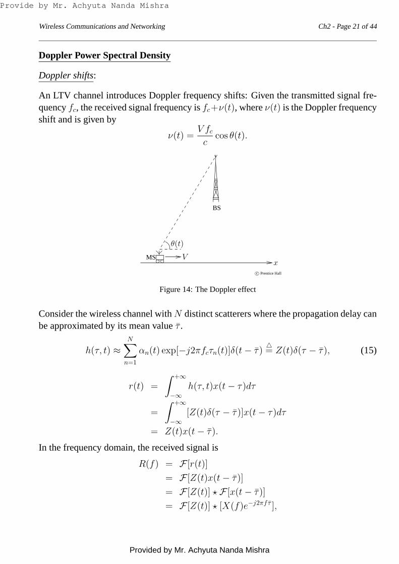
Doppler shifts:

An LTV channel introduces Doppler frequency shifts: Given the transmitted signalfre-quencyfc, the received signal frequency isfc+ν(t), whereν(t) is the Doppler frequencyshift and is given by

ν(t) =V fc

ccos θ(t).

c© Prentice Hall

θ(t)

VMS

BS

x

Figure 14: The Doppler effect

Consider the wireless channel withN distinct scatterers where the propagation delay canbe approximated by its mean valueτ .

h(τ, t) ≈N∑

n=1

αn(t) exp[−j2πfcτn(t)]δ(t − τ)= Z(t)δ(τ − τ), (15)

r(t) =

∫ +∞


=

∫ +∞

−∞[Z(t)δ(τ − τ)]x(t − τ)dτ

= Z(t)x(t − τ).

In the frequency domain, the received signal is

R(f) = F [r(t)]

= F [Z(t)x(t − τ)]

= F [Z(t)] ⋆ F [x(t − τ)]

= F [Z(t)] ⋆ [X(f)e−j2πfτ ],




=⇒ The channel indeed broadens the transmitted signal spectrum by introducing newfrequency components, a phenomenon referred to as frequency dispersion.

Doppler-spread function H(f, ν):

H(f, ν) is the channel gain associated with Doppler shiftν to the input signal componentat frequencyf .

R(f) =

∫ +∞

−∞X(f − ν)H(f − ν, ν)dν. (16)

Relation betweenH(f, t) andH(f, ν):

H(f, ν) = Ft[H(f, t)] =∫ +∞−∞ H(f, t)e−j2πvtdt

H(f, t) = F−1ν [H(f, ν)] =

∫ +∞−∞ H(f, ν)e+j2πνtdν

=⇒ being time-variant in the time domain can be equivalently described byhavingDoppler shifts in the frequency domain.




Autocorrelation function of H(f, ν):

ΦH(f1, f2, ν1, ν2)=

1

2E[H∗(f1, ν1)H(f2, ν2)

=

∫ ∫1

2E[H∗(f1, t1)H(f2, t2)]e

j2πν1t1e−j2πν2t2dt1dt2

WSSUS=

∫ ∫

φH(∆f, ∆t)e−j2π[ν2(t1+∆t)−ν1t1]d∆tdt1

(where∆f = f2 − f1 and∆t = t2 − t1)

=

∫

φH(∆f, ∆t)e−j2πν2∆td∆t

∫

e−j2π(ν2−ν1)t1dt1

= ΦH(∆f, ν2)δ(ν2 − ν1)

where

ΦH(∆f, ν) =

∫

φH(∆f, ∆t)e−j2πν∆td∆t

is the Fourier transform ofφH(∆f, ∆t) w.r.t. ∆t.

At ∆f = 0,

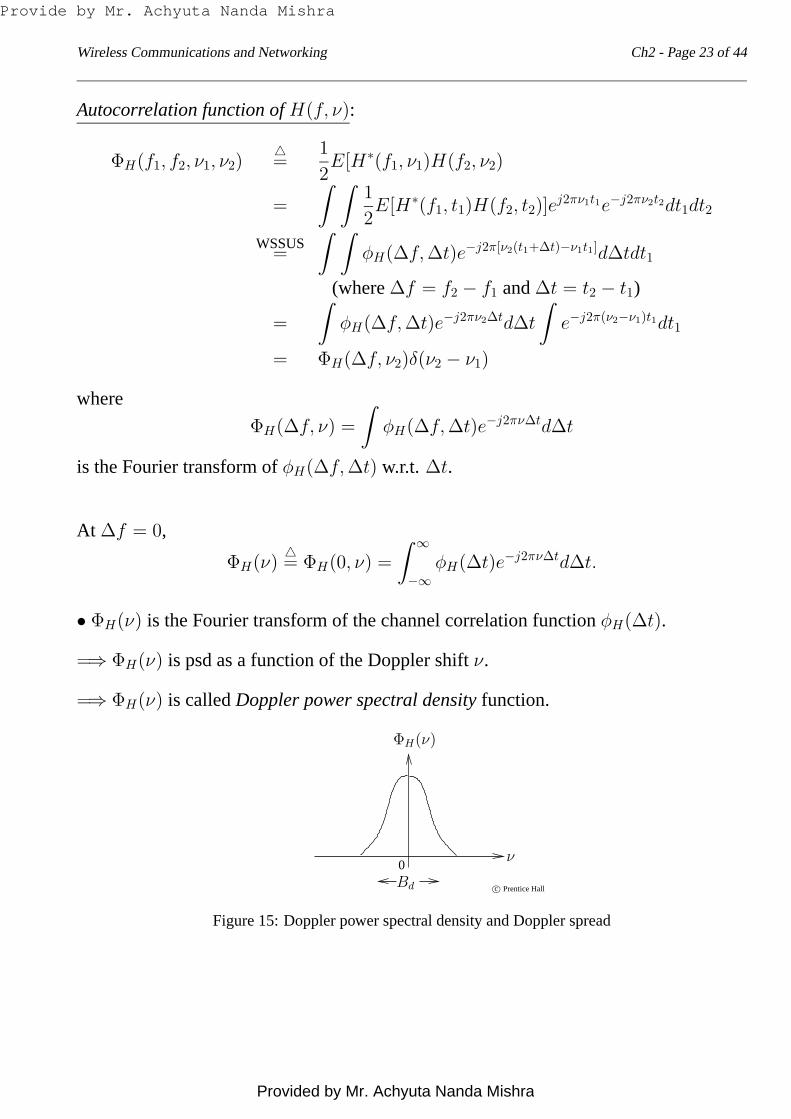
ΦH(ν)= ΦH(0, ν) =

∫ ∞

−∞φH(∆t)e−j2πν∆td∆t.

• ΦH(ν) is the Fourier transform of the channel correlation functionφH(∆t).

=⇒ ΦH(ν) is psd as a function of the Doppler shiftν.

=⇒ ΦH(ν) is calledDoppler power spectral density function.

0

c© Prentice HallBd

ν

ΦH(ν)

Figure 15: Doppler power spectral density and Doppler spread




• The nominal width of the Doppler psd,Bd, is called the Doppler spread.

• SinceφH(∆t) ↔ ΦH(ν),

(∆t)c ≈1

Bd.

• The mean Doppler shift is

ν =

∫νΦH(ν)dν

∫ΦH(ν)dν

and the rms Doppler spread is

σν = [

∫(ν − ν)2ΦH(ν)dν

∫ΦH(ν)dν

]1/2.

As an approximation, it is usually assumed that

Bd ≈ σν.




Example 2.3 Delay psd and frequency-correlation functionConsider a WSSUS channel whose time-variant impulse response is given by

h(τ, t) = exp(−τ/T )n(τ) cos(Ωt + Θ), τ ≥ 0,

whereT andΩ are constants,Θ is a random variable uniformly distributed in[−π, +π],andn(τ) is a random process independent ofΘ, with E[n(τ)] = µn andE[n(τ1)n(τ2)] =δ(τ1 − τ2).

a. Calculate the delay psd and the multipath delay spread.

b. Calculate the frequency correlation function and the channel coherence bandwidth.

c. Determine whether the channel exhibits frequency-selective fading for GSM sys-tems withT = 0.1 ms.

Solution:

a. From Eq. (11), we have

φh(τ) = F∆τ1

2E[h∗(τ, t)h(τ + ∆τ, t]

= F∆τ1

2E[n(τ)n(τ + ∆τ)]E[e−(2τ+∆τ)/T cos2(Ωt + Θ)], τ ≥ 0

= F∆τ1

4e−(2τ+∆τ)/T δ(∆τ)E[1 + cos(2Ωt + 2Θ)], τ ≥ 0

=1

4e−2τ/T , τ ≥ 0,

where

E[cos(2Ωt + 2Θ)] =

∫ +π

−π

cos(2Ωt + 2θ)1

2πdθ = 0.

For τ < 0, φh(τ) = 0.




The mean propagation delay is

τ =

∫ ∞0 τφh(τ)dτ∫ ∞

0 φh(τ)dτ=

∫ ∞0 τ 1

4e−2τ/Tdτ

∫ ∞0

14e

−2τ/Tdτ=

T

2

and the multipath delay spread is

Tm ≈ στ = [

∫(τ − τ)2φh(τ)dτ

∫φh(τ)dτ

]1/2 = [

∫τ 2φh(τ)dτ

∫φh(τ)dτ

− τ 2]1/2 =T

2.

b. The frequency correlation function is

φH(∆f) = F [φh(τ)]

=

∫ ∞

0

1

4e−2τ/Te−j2π(∆f)τdτ

=T

8 + j8πT (∆f).

The coherence bandwidth is

(∆f)c ≈ 1/Tm =2

T.

c. With T = 0.1 ms, we have(∆f)c = 20 kHz. The GSM channels have a bandwidthof 200 kHz. Since(∆f)c ≪ 200 kHz, the channel fading is frequency selective.

¤




Example 2.4 Doppler psdFor the channel specified in Example 2.3 withΩ = 10π, find

a. the Doppler psd,

b. the mean Doppler shift and the rms Doppler spread,

c. the channel coherence time, and

d. whether the channel exhibits slow fading for GSM systems.

Solution:

a. The Doppler psd can be calculated by taking the Fourier transform of the time cor-relation functionφH(∆t). In this way, we need to calculate the correlation functionφh(τ, ∆t) first. For the WSS channel, we have forτ ≥ 0

φh(τ, ∆t)

= F∆τ1

2E[h∗(τ, t)h(τ + ∆τ, t + ∆t)]

= F∆τ1

2E[e−τ/Tn(τ) cos(Ωt + Θ) · e−(τ+∆τ)/Tn(τ + ∆τ) cos(Ωt + Ω∆t + Θ)]

= F∆τ1

4e−(2τ+∆τ)/TE[n(τ)n(τ + ∆τ)]E[cos(Ω∆t) + cos(2Ωt + Ω∆t + 2Θ)]

= F∆τ1

4e−(2τ+∆τ)/T δ(∆τ) cos(Ω∆t)

=1

4e−2τ/T cos(Ω∆t), τ ≥ 0.

The time correlation function is then

φH(∆t) = φH(∆f, ∆t)|∆f=0

=

∫ +∞

−∞φh(τ, ∆t)dτ

=1

4cos(Ω∆t)

∫ +∞

0

e−2τ/Tdτ

=T

8cos(Ω∆t).




The Doppler psd is

ΦH(ν) = F [φH(∆t)]

= F [T

8cos(Ω∆t)]

=T

16[δ(2πν − Ω) + δ(2πν + Ω)].

That is, the channel introduces two Doppler shifts,±Ω/2π = ±5 Hz, with equalpsd.

b. The mean Doppler shift is zero as the two Doppler shifts are negative of each otherand have the same psd. The rms Doppler spread is

σν = ∫ +∞−∞ ν2 · T

16 [δ(2πν − Ω) + δ(2πν + Ω)]dν∫ +∞−∞

T16 [δ(2πν − Ω) + δ(2πν + Ω)]dν

1/2

= T16 [(

Ω2π)2 + (− Ω

2π)2]T16 [1 + 1]

1/2

=Ω

2π,

which is 5 Hz.

c. The coherence time is

(∆t)c ≈1

σν= 0.2 s.

d. In GSM systems, the data rateRs = 270.833 kbps, which corresponds to a symbolinterval

Ts =1

Rs≈ 3.7 × 10−6 s.

SinceTs ≪ (∆t)c, the channel exhibits slow fading.

¤




2.4 Large-Scale Path Loss and Shadowing

Consider a flat fading channel with the channel impulse response

h(τ, t) ≈ h(τ , t)= g(t)δ(τ − τ).


r(t) =

∫ +∞

−∞h(τ, t)x(t − τ)dτ ≈ g(t)x(t − τ).

Flat fading channel

c© Prentice Hall

x(t) r(t) = g(t)x(t − τ)

h(τ, t) = g(t)δ(τ − τ)




50 100 150 200 250 300 350 400 450 500−120

−115

−110

−105

−100

−95

−90

−85

−80

−75

−70

Am

plitu

de fa

ding

|g(t

)| (

dB)

time (ms)

Prentice Hall

local mean

(a) Overall amplitude fading|g(t)| (dB)

50 100 150 200 250 300 350 400 450 500−35

−30

−25

−20

−15

−10

−5

0

5

10

15

Sho

rt−

term

am

plitu

de fa

ding

|Z(t

)| (

dB)

time (ms)

Prentice Hall

local mean

(b) Short-term amplitude fading|Z(t)| (dB)

Figure 16: Representation of long-term and short-term fading components




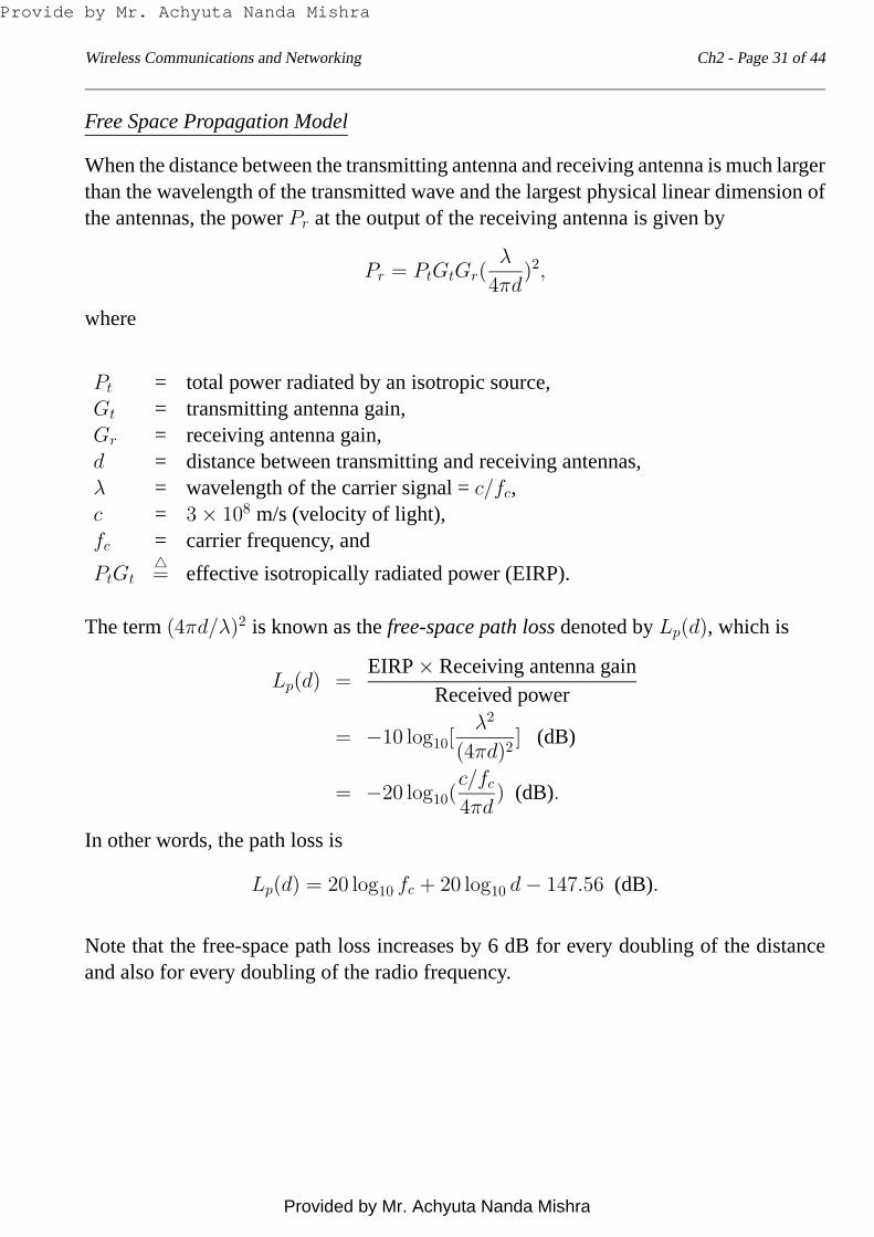
Free Space Propagation Model

When the distance between the transmitting antenna and receiving antenna is muchlargerthan the wavelength of the transmitted wave and the largest physical lineardimension ofthe antennas, the powerPr at the output of the receiving antenna is given by

Pr = PtGtGr(λ

4πd)2,

where

Pt = total power radiated by an isotropic source,Gt = transmitting antenna gain,Gr = receiving antenna gain,d = distance between transmitting and receiving antennas,λ = wavelength of the carrier signal =c/fc,c = 3 × 108 m/s (velocity of light),fc = carrier frequency, and

PtGt= effective isotropically radiated power (EIRP).

The term(4πd/λ)2 is known as thefree-space path loss denoted byLp(d), which is

Lp(d) =EIRP× Receiving antenna gain

Received power

= −10 log10[λ2

(4πd)2] (dB)

= −20 log10(c/fc

4πd) (dB).

In other words, the path loss is

Lp(d) = 20 log10 fc + 20 log10 d − 147.56 (dB).

Note that the free-space path loss increases by 6 dB for every doubling of the distanceand also for every doubling of the radio frequency.




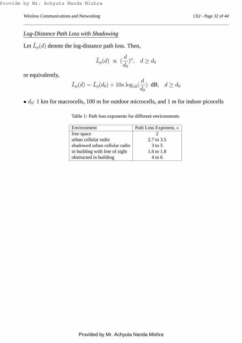
Log-Distance Path Loss with Shadowing

Let Lp(d) denote the log-distance path loss. Then,

Lp(d) ∝ (d

d0)κ, d ≥ d0

or equivalently,

Lp(d) = Lp(d0) + 10κ log10(d

d0) dB, d ≥ d0

• d0: 1 km for macrocells, 100 m for outdoor microcells, and 1 m for indoor picocells

Table 1: Path loss exponents for different environments

Environment Path Loss Exponent,κfree space 2urban cellular radio 2.7 to 3.5shadowed urban cellular radio 3 to 5in building with line of sight 1.6 to 1.8obstructed in building 4 to 6




• Shadowing: As the mobile moves in uneven terrain, it often travels into a propagationshadow behind a building or a hill or other obstacle much larger than the wavelength ofthe transmitted signal, and the associated received signal level is attenuated significantly.

• A log-normal distribution is a popular model for characterizing the shadowing process.

Let ǫ(dB) be a zero-mean Gaussian distributed random variable (in dB) with standardde-viationσǫ (in dB). The pdf ofǫ(dB) is given by

fǫ(dB)(x) =1√2πσǫ

exp(− x2

2σ2ǫ

).

Let Lp(d) denote the overall long-term fading (in dB). Then,

Lp(d) = Lp(d) + ǫ(dB)

= Lp(d0) + 10κ log10(dd0

) + ǫ(dB) (dB).

• ǫ(dB) follows the Gaussian (normal) distribution=⇒ ǫ in linear scale is said to follow alog-normal distribution with pdf given by

fǫ(y) =20/ ln 10√

2πyσǫ

exp[−(20 log10 y)2

2σ2ǫ

].

• σǫ: 8 dB for an outdoor cellular system and 5 dB for an indoor environment.




2.5 Small-Scale Multipath Fading

Consider a flat fading channel withN distinct scatterers:

r(t) =N∑

n=1

αn(t)e−j2πfcτn(t)x(t − τn(t))

≈ [N∑

n=1

αn(t)e−j2πfcτn(t)]x(t − τ).

The complex gain of the channel is

Z(t) =N∑

n=1

αn(t)e−j2πfcτn(t)

= Zc(t) − jZs(t)

where

Zc(t) =N∑

n=1

αn(t) cos θn(t)

Zs(t) =N∑

n=1

αn(t) sin θn(t)

andθn(t) = 2πfcτn(t).

Also,Z(t) = α(t) exp[jθ(t)]

whereα(t) =

√

Z2c (t) + Z2

s (t), θ(t) = tan−1[Zs(t)/Zc(t)].




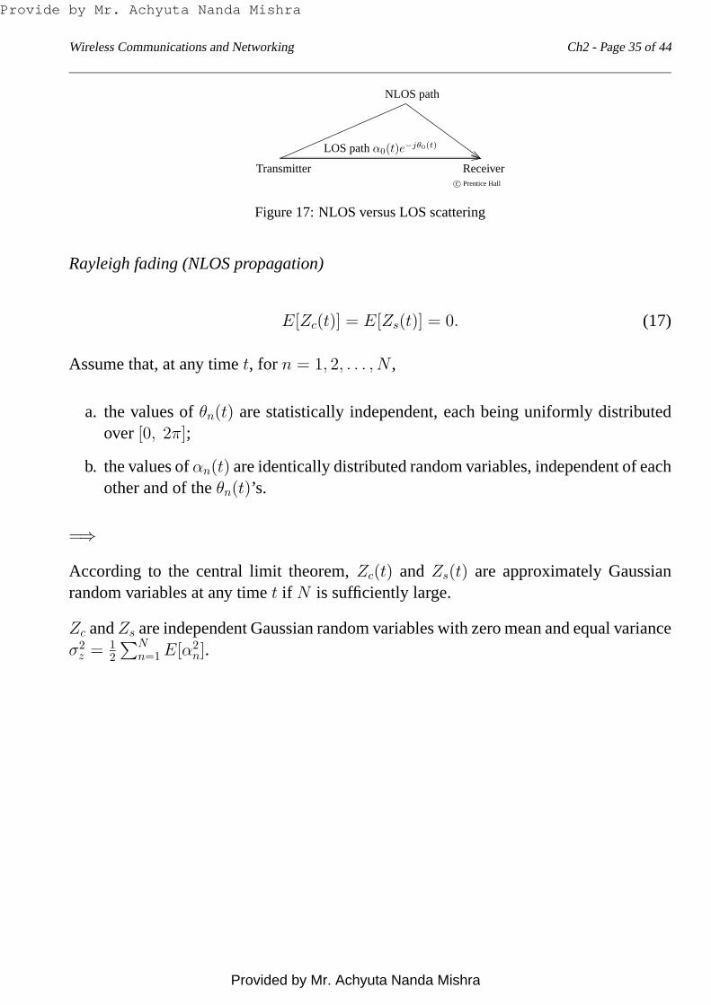
c© Prentice Hall

Transmitter Receiver

LOS pathα0(t)e−jθ0(t)

NLOS path

Figure 17: NLOS versus LOS scattering

Rayleigh fading (NLOS propagation)

E[Zc(t)] = E[Zs(t)] = 0. (17)

Assume that, at any timet, for n = 1, 2, . . . , N ,

a. the values ofθn(t) are statistically independent, each being uniformly distributedover[0, 2π];

b. the values ofαn(t) are identically distributed random variables, independent of eachother and of theθn(t)’s.

=⇒

According to the central limit theorem,Zc(t) and Zs(t) are approximately Gaussianrandom variables at any timet if N is sufficiently large.

Zc andZs are independent Gaussian random variables with zero mean and equal varianceσ2

z = 12

∑Nn=1 E[α2

n].




=⇒

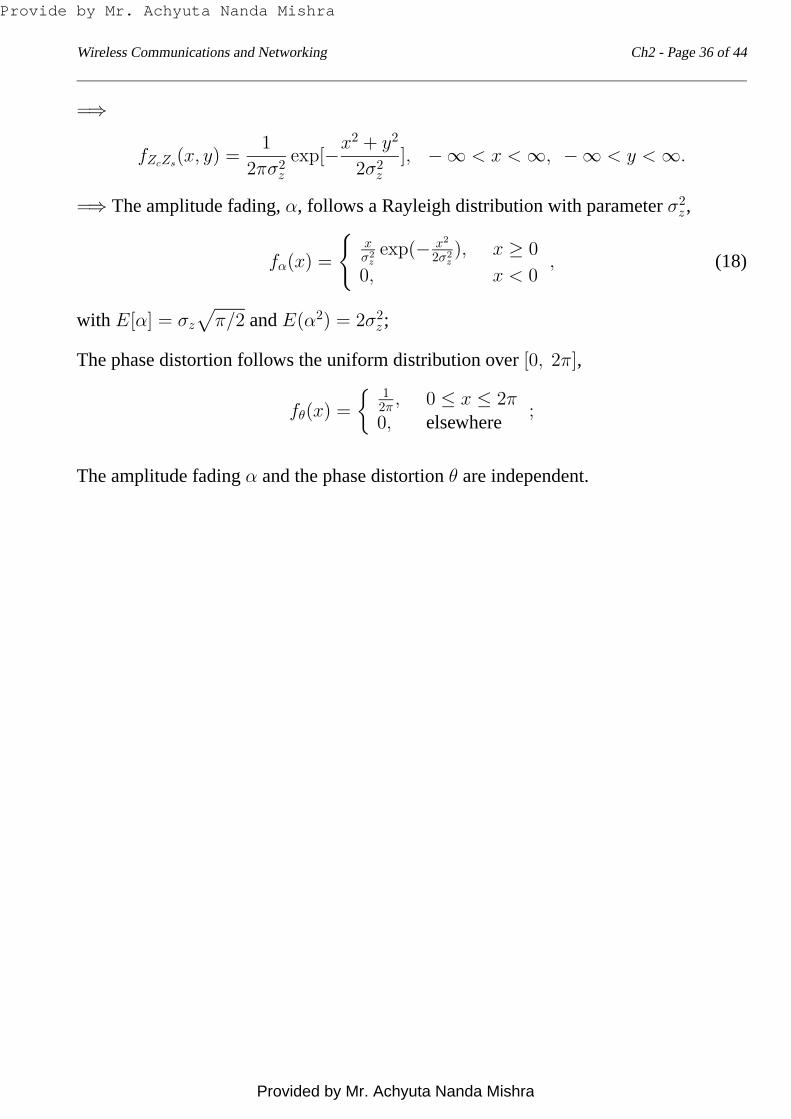
fZcZs(x, y) =

1

2πσ2z

exp[−x2 + y2

2σ2z

], −∞ < x < ∞, −∞ < y < ∞.

=⇒ The amplitude fading,α, follows a Rayleigh distribution with parameterσ2z ,

fα(x) =

xσ2

zexp(− x2

2σ2z), x ≥ 0

0, x < 0, (18)

with E[α] = σz

√

π/2 andE(α2) = 2σ2z ;

The phase distortion follows the uniform distribution over[0, 2π],

fθ(x) =

12π , 0 ≤ x ≤ 2π0, elsewhere

;

The amplitude fadingα and the phase distortionθ are independent.




Rician Fading (LOS propagation)

Z(t) = Zc(t) − jZs(t) + Γ(t),

whereΓ(t) = α0(t)e−jθ0(t) is the deterministic LOS component.

E[Z(t)] = Γ(t) 6= 0.

The distribution of the envelope at any timet is given by the Rayleigh distribution mod-ified by

a. a factor containing a non-centrality parameter, and

b. a zero-order modified Bessel function of the first kind.

The resultant pdf for the amplitude fading at anyt, α, is known as the Rician distribution,given by

fα(x) =x

σ2z

exp(− x2

2σ2z

)

︸︷︷︸

Rayleigh

· exp− α20

2σ2z

· I0(α0x

σ2z

)

︸︷︷︸

modifier

=x

σ2z

exp(−x2 + α20

2σ2z

)I0(α0x

σ2z

), x ≥ 0,

whereα0 isα0(t) at anyt, α20 is the power of the LOS component and is the non-centrality

parameter,I0(·) is the zero-order modified Bessel function of the first kind and is givenby

I0(x) =1

2π

∫ 2π

0

exp(x cos θ)dθ.




• TheK factor:

K∆=

Power of the LOS componentTotal power of all other scatterers

=α2

0

2σ2z

.

K → 0 =⇒ the Rician distribution→ the Rayleigh distribution;

K → ∞ =⇒ the Rician fading channel→ an AWGN channel.

0 1 2 3 4 5 60

0.1

0.2

0.3

0.4

0.5

0.6

0.7

x

f α (x)

Prentice Hall

K=−∞ dBK=−5 dBK=0 dBK=5 dB

Figure 18: Rayleigh and Rician fading distributions withσz = 1




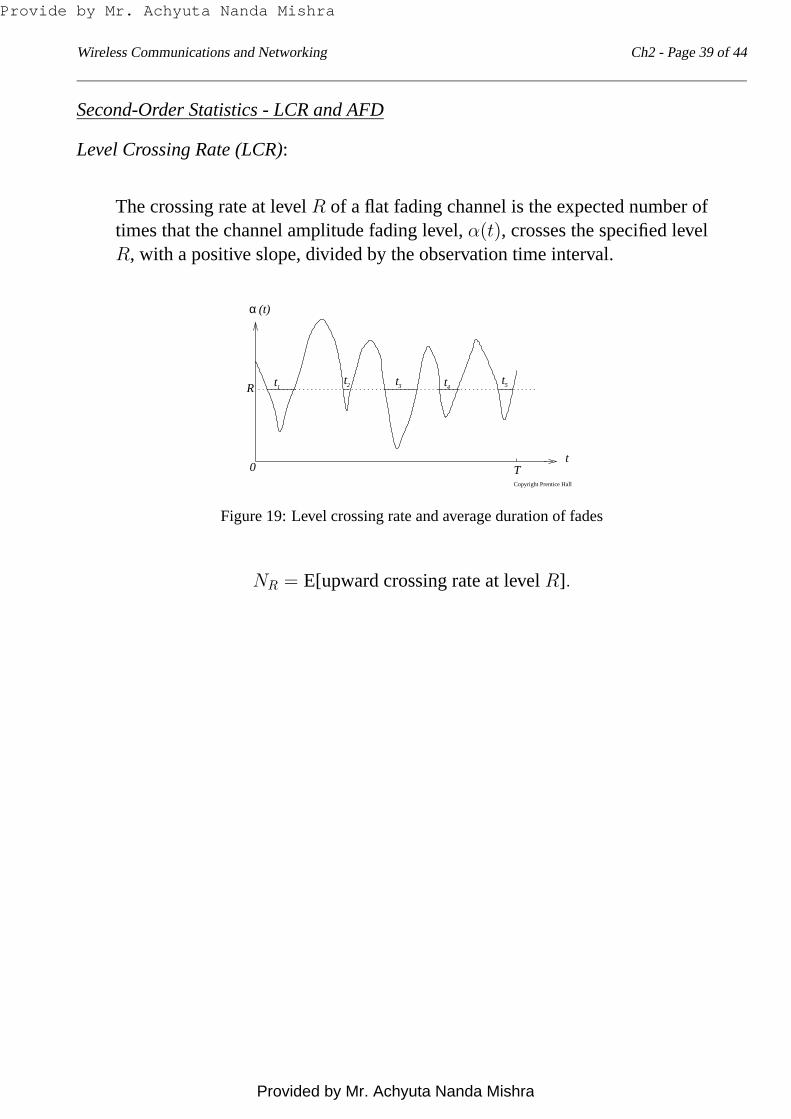
Second-Order Statistics - LCR and AFD

Level Crossing Rate (LCR):

The crossing rate at levelR of a flat fading channel is the expected number oftimes that the channel amplitude fading level,α(t), crosses the specified levelR, with a positive slope, divided by the observation time interval.

α


t

T

t t t t2 3 51 4

0

(t)

t

R

Figure 19: Level crossing rate and average duration of fades

NR = E[upward crossing rate at levelR].




Let α = dα(t)/dt denote the amplitude fading rate and letfαα(x, y) denote the joint pdfof the amplitude fadingα(t) and its derivativeα(t) at any timet. Then,

NR =

∫ ∞

0

yfαα(x, y)|x=Rdy.

For the Rayleigh fading environment,

fαα(x, y) =x

√

2πσ2ασ2

z

exp[−1

2(x2

σ2z

+y2

σ2α

)], x ≥ 0, −∞ < y < ∞,

where

σ2α =

1

2(2πνm)2σ2

z

andνm is the maximum Doppler shift. The LCR is

NR =

∫ ∞

0

y · R√

2πσ2ασ2

z

exp[−1

2(R2

σ2z

+y2

σ2α

)]dy

=√

2πνm(R√2σz

) exp(− R2

2σ2z

).

Letting

ρ =R√2σz

we haveNR =

√2πνmρ exp(−ρ2).




−10 −8 −6 −4 −2 0 2 4 6 8 1010

−4

10−3

10−2

10−1

100

ρ (dB)

Nor

mal

ized

leve

l cro

ssin

g ra

te, ρ

exp

(−ρ

2 )

Prentice Hall

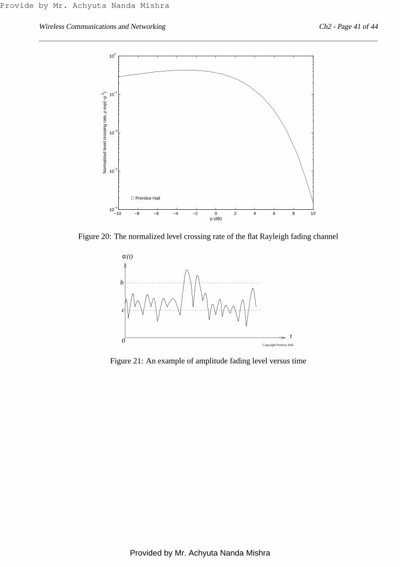
Figure 20: The normalized level crossing rate of the flat Rayleigh fading channel


α

t0

b

c

(t)

Figure 21: An example of amplitude fading level versus time




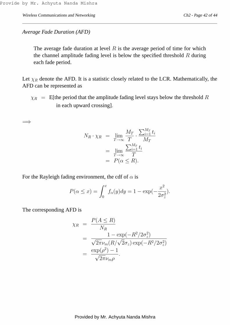
Average Fade Duration (AFD)

The average fade duration at levelR is the average period of time for whichthe channel amplitude fading level is below the specified thresholdR duringeach fade period.

Let χR denote the AFD. It is a statistic closely related to the LCR. Mathematically, theAFD can be represented as

χR = E[the period that the amplitude fading level stays below the thresholdR

in each upward crossing].

=⇒

NR · χR = limT→∞

MT

T·∑MT

i=1 tiMT

= limT→∞

∑MT

i=1 tiT

= P (α ≤ R).

For the Rayleigh fading environment, the cdf ofα is

P (α ≤ x) =

∫ x

0

fα(y)dy = 1 − exp(− x2

2σ2z

).

The corresponding AFD is

χR =P (A ≤ R)

NR

=1 − exp(−R2/2σ2

z)√2πνm(R/

√2σz) exp(−R2/2σ2

z)

=exp(ρ2) − 1√

2πνmρ.




−10 −8 −6 −4 −2 0 2 4 6 8 1010

−1

100

101

102

103

104

ρ (dB)

Nor

mal

ized

ave

rage

fade

dur

atio

n, [e

xp(ρ

2 )−1]

/ ρ

Prentice Hall

Figure 22: The normalized average fade duration of the flat Rayleigh fading channel




Example 2.8 The LCRNR and AFD χR

Consider a mobile cellular system in which the carrier frequency isfc = 900 MHz andthe mobile travels at a speed of 24 km/h. Calculate the AFD and LCR at the normalizedlevelρ = 0.294.

Solution:

At fc = 900 MHz, the wavelength isλ = cfc

= 3×108

900×106 = 13 m. The velocity of the

mobile isV = 24 km/h = 6.67 m/s. The maximum Doppler frequency isνm = V/λ =6.671/3 = 20 Hz. The average duration of fades below the normalized levelρ = 0.294 is

χR =eρ2 − 1√2πνmρ

=e(0.294)2 − 1√

2π × 20 × 0.294= 0.0061 s.

The level crossing rate atρ = 0.294 is

NR =√

2πνmρe−ρ2

=√

2π × 20 × 0.294e−(0.294)2

= 16 upcrossings/second.

¤



Education

Characterization of the Wireless Channel