Embed Size (px)
Citation preview

The Value of Travel Time:
Random Utility vs Random Valuation
Manuel Ojeda-Cabral, Stephane Hess & Richard Batley
ITS, University of Leeds
Manuel Ojeda-Cabral
Research Fellow
ITS, University of Leeds
Transportation Research Board – 94th Annual meeting, January 2015

The Value of Travel Time Changes
The Value of Travel Time Changes
Focus on national studies
Value of travel time: key input for appraisal of projects

The Value of Travel Time Changes
Numerous issues remain unresolved. Are we doing
anything wrong? How can we do things better?
Our contribution:
Comparative analysis of some elements
of two important national studies.

The Value of Travel Time Changes
Imagine a travel choice scenario such as follows:
TRAVEL
OPTION 1
TRAVEL
OPTION 2
COST £5 £10
TIME 60 min. 30 min.
Implicit valuation threshold:
|10 − 5|
|30 − 60|∗ 60 = 10 £/hour
(known as: Boundary VTTC)
Simple time-cost
trade-offs in all SP
tasks.
Assumption: We can find it in people’s choices that involve a trade-off
between money and time.

Two national studies on the Value of Time
Why is this analysis interesting?
0. Travellers & context:
Different (potentially)
1. Microeconomic theory
2. Design: Identical*
3. Models: Different
Vs.
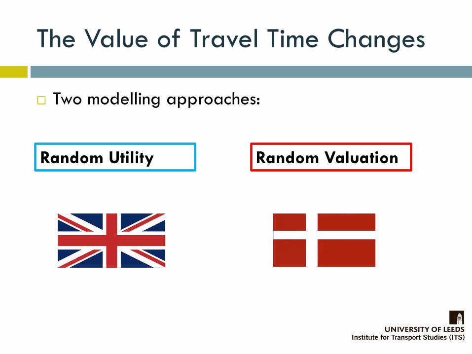
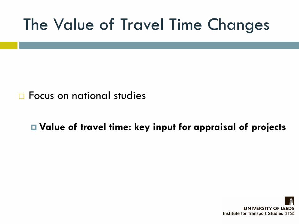
Two modelling approaches:
The Value of Travel Time Changes
Random Utility Random Valuation
Two modelling approaches:
The Value of Travel Time Changes
Random Utility Random Valuation
Travel choice scenario:
TRAVEL
OPTION 1
TRAVEL
OPTION 2
COST £5 £10
TIME 60 min. 30 min.
Implicit valuation threshold:
|10 − 5|
|30 − 60|∗ 60 = 10 £/hour
(known as: Boundary VTTC)
𝑦 = 1 𝑉𝑇𝑇𝐶 < BVTTC + 𝜀
𝑦 = 1 𝑉1 > V2 + 𝜀
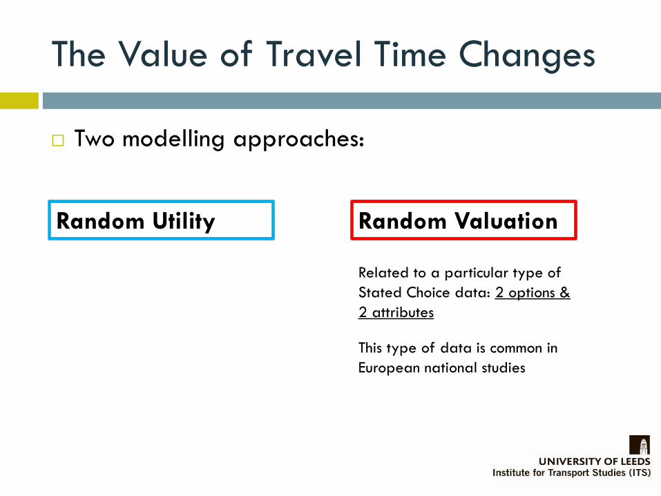
Two modelling approaches:
The Value of Travel Time Changes
Random Utility Random Valuation
Related to a particular type of
Stated Choice data: 2 options &
2 attributes
This type of data is common in
European national studies

Theoretical relationship?
The Value of Travel Time Changes
Random Utility Random Valuation

Theoretical relationship:
Both derived from Microeconomic Theory
𝑈𝑖 = (𝑉𝑖 , 𝜀𝑖)
where: 𝑉𝑖 = 𝛽𝑐𝑐𝑖 + 𝛽𝑡𝑡𝑖
𝑉𝑇𝑇𝐶 =𝛽𝑡
𝛽𝑐
Difference: how is the 𝜀𝑖 introduced?
The Value of Travel Time Changes
Random Utility Random Valuation

Theoretical relationship: Deterministic domain
If the slow option 1 is chosen, then VTTC < BVTTC:
The Value of Travel Time Changes
Random Utility Random Valuation
𝛽𝑡 ∗ 𝑡1 + 𝛽𝑐 ∗ 𝑐1 > 𝛽𝑡∗ 𝑡2 + 𝛽𝑐 ∗ 𝑐2
𝛽𝑡 ∗ 𝑡1 − 𝑡2 > −𝛽𝑐 ∗ (𝑐1 − 𝑐2)
𝛽𝑡
𝛽𝑐< −
(𝑐1−𝑐2)
𝑡1−𝑡2
VTTC < BVTTC
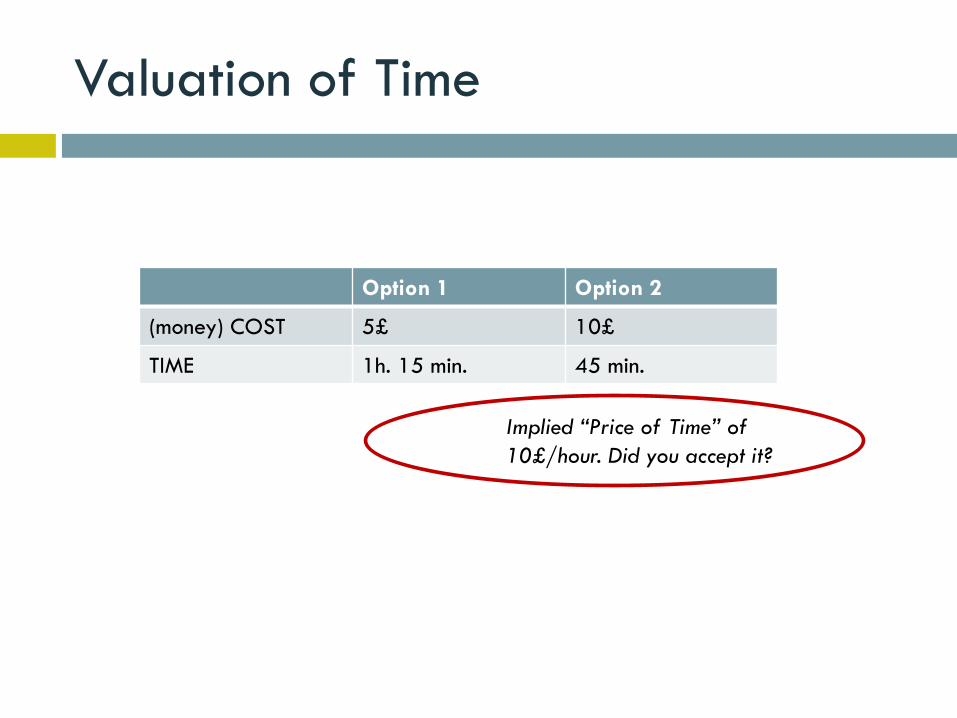
Valuation of Time
Option 1 Option 2
(money) COST 5£ 10£
TIME 1h. 15 min. 45 min.
Implied “Price of Time” of
10£/hour. Did you accept it?
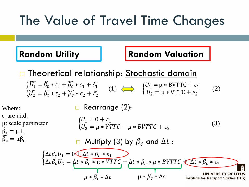
Theoretical relationship: Stochastic domain
The Value of Travel Time Changes
Random Utility Random Valuation
𝑈1 = 𝛽𝑡 ∗ 𝑡1 + 𝛽𝑐 ∗ 𝑐1 + 𝜀1 𝑈2 = 𝛽𝑡 ∗ 𝑡2 + 𝛽𝑐 ∗ 𝑐2 + 𝜀2
(1) 𝑈1 =μ ∗ BVTTC + 𝜀1𝑈2 = μ ∗ VTTC + 𝜀2
(2)
Where:
εi are i.i.d.
μ: scale parameter βt = μβt βc = μβc
𝑈1 =0 + 𝜀1𝑈2 = 𝜇 ∗ 𝑉𝑇𝑇𝐶 − 𝜇 ∗ 𝐵𝑉𝑇𝑇𝐶 + 𝜀2
(3)
Rearrange (2):
Multiply (3) by 𝛽𝑐 and ∆𝑡 :
∆𝑡𝛽𝑐𝑈1 =0 + ∆𝑡 ∗ 𝛽𝑐 ∗ 𝜀1∆𝑡𝛽𝑐𝑈2 = ∆𝑡 ∗ 𝛽𝑐 ∗ 𝜇 ∗ 𝑉𝑇𝑇𝐶 − ∆𝑡 ∗ 𝛽𝑐 ∗ 𝜇 ∗ 𝐵𝑉𝑇𝑇𝐶 + ∆𝑡 ∗ 𝛽𝑐 ∗ 𝜀2
μ ∗ 𝛽𝑐 ∗ ∆𝑐𝜇 ∗ 𝛽𝑡 ∗ ∆𝑡

Theoretical relationship: Stochastic domain
The Value of Travel Time Changes
Random Utility Random Valuation
𝑈1 = 𝛽𝑡 ∗ 𝑡1 + 𝛽𝑐 ∗ 𝑐1 + 𝜀1 𝑈2 = 𝛽𝑡 ∗ 𝑡2 + 𝛽𝑐 ∗ 𝑐2 + 𝜀2
𝑈1 =μ ∗ BVTTC + 𝜀1𝑈2 = μ ∗ VTTC + 𝜀2
𝜀𝑖 = ∆𝑡 ∗ 𝛽𝑐 ∗ 𝜀𝑖
Difference: particular
form of heteroskedastic
errors

Empirical comparison?
The Value of Travel Time Changes
Random Utility Random Valuation

Design & dataset in each country:
Common SC design, implemented slightly differently: 1. Travellers &
context:
Different
2. Design:
Identical*
TRAVEL
OPTION 1
TRAVEL
OPTION 2
COST change
(∆c)
100 pence 0
TIME change
(∆t)
-15 min. 0
TRAVEL
OPTION 1
TRAVEL
OPTION 2
COST 400 pence 300 pence
TIME 30 min. 45 min.
(Illustrative values in £, instead of DKK, for comparison)
Two national studies on the Value of Time

Empirical comparison?
1) Linear
2) in Logarithms
3) + observed heterogeneity
4) + random heterogeneity
The Value of Travel Time Changes
Random Utility Random Valuation

The Value of Travel Time Changes
Random Utility Random Valuation
𝑈1 = 𝛽𝑐(𝛽𝑡𝛽𝑐
∗ 𝑡1 + 𝑐1 + 𝜀1
𝑈2 = 𝛽𝑐(𝛽𝑡𝛽𝑐
∗ 𝑡2 + 𝑐2) + 𝜀2 𝑈1 =μ ∗ BVTTC + 𝜀1𝑈2 = 𝜇 ∗ 𝑉𝑇𝑇𝐶 + 𝜀2
𝑈1
′ = )μ ∗ 𝑙𝑛(VTTC ∗ 𝑡1 + 𝑐1 + 𝜀1′
𝑈2′ = 𝜇 ∗ 𝑙𝑛(𝑉𝑇𝑇𝐶 ∗ 𝑡2 + 𝑐2) + 𝜀2
′ 𝑈1
′ = )μ ∗ l n( BVTTC + 𝜀1′
𝑈2′ = 𝜇 ∗ 𝑙 𝑛( 𝑉𝑇𝑇𝐶) + 𝜀2
′
; VTTC =𝛽𝑡𝛽𝑐
= β0
VTTC = 𝑒 β0+β𝐵𝐶l n(
𝐶𝐶0
)+β𝐵𝑇l n(𝑇𝑇0
)+β𝐼l n(𝐼𝐼0
1
2
3
4 VTTC = 𝑒β0+β𝐵𝐶 ln
𝐶𝐶0
+β𝐵𝑇 ln𝑇𝑇0
+β𝐼 ln𝐼𝐼0
+𝒖

The Value of Travel Time Changes
1. Linear 2. Logarithms
RU RV RU RV
Est. t-test Est. t-test Est. t-test Est. t-test
βc 1 na na na 1 na na na
β0 4.89 18.64 3.22 11.76 3.71 22.38 2.75 23.71
μ -0.0138 -20.81 0.115 24.03 -6.42 -23.12 0.79 33.15
VTTC
pence/min
4.89 3.22 3.71 4.28
Obs. 10598 10598 10598 10598
Parameters 2 2 2 2
Null LL -7345.974 -7345.974 -7345.974 -7345.974
Final LL -6746.152 -6570.224 -6690.042 -6465.961
Adj. Rho20.081 0.105 0.089 0.120

The Value of Travel Time Changes
3. Logarithms + Covariates 4. Log + Covariates + Random Het.
RU RV RU RV
Est. t-test Est. t-test Est. t-test Est. t-test
βc 1 na na na 1 na na na
β0 1.70 30.23 1.30 28.25 1.58 28.64 1.29 28.11
μ 7.39 25.26 0.859 34.24 11.5 24.06 1.09 33.00
βBC 0.470 8.78 0.431 7.57 0.431 7.45 0.428 25.29
βBT -0.362 -4.81 -0.196 -2.68 -0.279 -3.50 -0.189 -2.61
βI 0.273 5.13 0.411 8.06 0.344 6.40 0.382 7.77
σ na na na na 1.07 21.22 1.11 25.29
VTTC pence/min5.47 4.85 8.61 6.72
Obs. 10598 10598 10598 10598
Parameters 5 5 6 6
Null LL -7345.974 -7345.974 -7345.974 -7345.974
Final LL -6607.502 -6300.028 -6306.561 -5910.137
Adj. Rho20.100 0.142 0.141 0.195
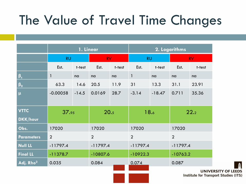
The Value of Travel Time Changes
1. Linear 2. Logarithms
RU RV RU RV
Est. t-test Est. t-test Est. t-test Est. t-test
βc 1 na na na 1 na na na
β0 63.3 14.6 20.5 11.9 31 13.3 31.1 23.91
μ -0.00058 -14.5 0.0169 28.7 -3.14 -18.47 0.711 35.36
VTTC
DKK/hour
37.95 20.5 18.6 22.2
Obs. 17020 17020 17020 17020
Parameters 2 2 2 2
Null LL -11797.4 -11797.4 -11797.4 -11797.4
Final LL -11378.7 -10807.6 -10922.3 -10763.2
Adj. Rho2 0.035 0.084 0.074 0.087

The Value of Travel Time Changes
3. Logarithms + Covariates 4. Log + Covariates + Random Het.
RU RV RU RV
Est. t-test Est. t-test Est. t-test Est. t-test
βc 1 na na na 1 na na na
β0 4.33 62.25 3.89 87.25 4.12 68.27 3.89 84.77
μ 4.41 20.37 0.768 36.3 10.3 24.4 1.06 34.84
βBC 0.571 6.51 0.701 9.44 0.581 7.00 0.705 9.23
βBT -0.48 -3.87 -0.643 -6.06 -0.451 -3.67 -0.633 -5.77
βI 0.501 6.63 0.638 9.76 0.611 8.47 0.633 9.74
σ na na na na 1.49 26.8 1.47 30.21
VTTC DKK/hour45.57 26.85 112.08 86.45
Obs. 17020 17020 17020 17020
Parameters 5 5 6 6
Null LL -11797.4 -11797.4 -11797.4 -11797.4
Final LL -10748.8 -10313.8 -9690.48 -9185.81
Adj. Rho2 0.088 0.125 0.178 0.221

The Value of Travel Time
Approx.
current
UK VTTC
0
1
2
3
4
5
6
7
8
9
10
Base Ln Ln+Cov Ln+Cov+Rand
VTTC(p/min)
Model extension
Mean Value of Time across models – UK data
RU approach
RV approach
RandomValuation > RandomUtility (model fit)
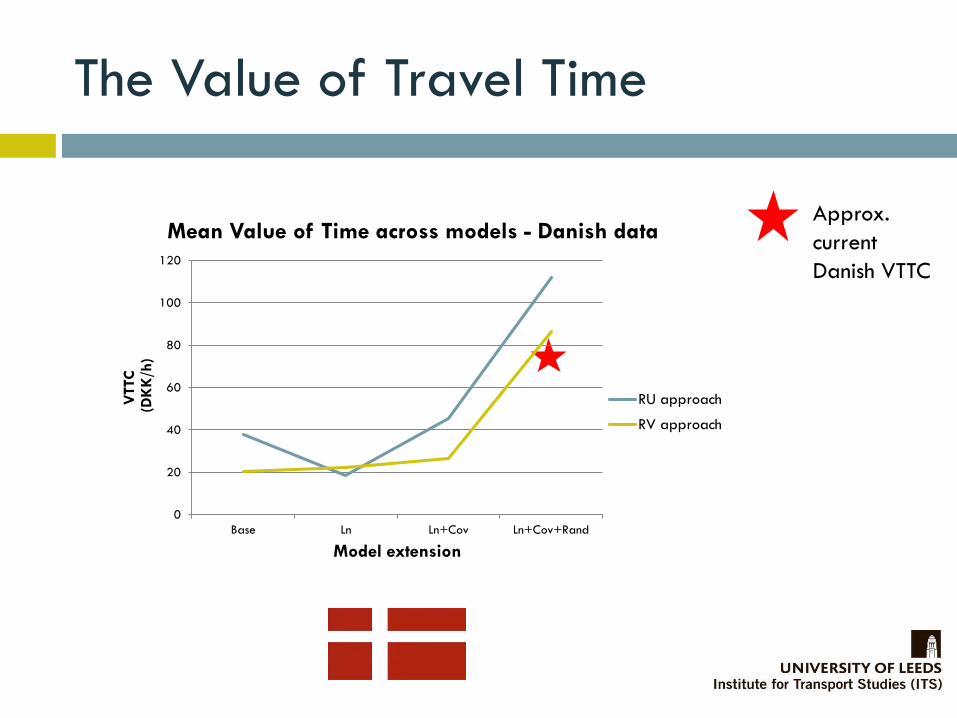
The Value of Travel Time
Approx.
current
Danish VTTC
0
20
40
60
80
100
120
Base Ln Ln+Cov Ln+Cov+Rand
VTTC
(DK
K/h
)
Model extension
Mean Value of Time across models - Danish data
RU approach
RV approach

The Value of Travel Time Changes
Some results:
The choice of approach matters.
Theoretically, none of the approaches is preferred.
Empirically:
RandomValuation > RandomUtility (model fit)
Lower Value of Time using RV approach
Similar pattern across models in UK & Denmark
The Value of Travel Time Changes
Some issues and recommendations:
Risk of significant biases on VTTC depending
on the form of error heteroskedasticity selected.
RV preferred if feasible: e.g. with simple
2options&2attributes experiments.
RU approach: likely to have heteroskedastic
errors that need correction.
Test both linear and logs specifications.
The Value of Travel Time Changes
Some questions:
Why is the VTTC always lower with the RV approach?
Validity of results using Random Utility approach? Always
worse model fit. What should we do in more complex
choice SC experiments?
Why are individuals’ preferences so similar in two
different countries? What is the role of stated choice
design on results?
Thanks
Manuel Ojeda-CabralResearch Fellow