What Determines Capital Inflows?:An Empirical Analysis for Chile†

Rómulo A. Chumacero *

Raúl Labán M.**

Felipe Larraín B.***

ABSTRACT

This paper presents an empirical investigation of the determinants of short- and long-termnet private capital inflows to Chile between 1985 and 1994. It is shown that the factorsdetermining each type of flow are quite different in nature. Long-term flows tend torespond to structural (domestic) variables of the economy and are not sensitive to short-term arbitrage conditions or to policy measures aimed at affecting the interest rate gap.Short-term flows react strongly to arbitrage conditions, a combination of internal andexternal factors, and to policy variables, but are not sensitive to structural factors.

In order to capture adequately the dynamic properties of these inflows, different regimesare taken into account. In particular, full sample stable specifications are strongly rejectedin most cases, while threshold processes are preferred to Markov switching-regimemodels. The effects of selective capital controls on short-term inflows are derived bysplitting short-term inflows into two series: one that is subject to these controls and onethat is not. Significant differences are found between the two series.

Keywords: Capital Inflows, Selective Controls, Threshold Process, Markov SwitchingRegimes, Bootstrap.

JEL Classification: F21, F47, C22.

Revised March 1997

† A previous version of this paper was presented to the conference “The Return of Private Capital to LatinAmerica”, organized by the Catholic University of Chile. We benefited from the comments of severalconference participants, with special thanks to Felipe Morandé and Patricio Rojas for their suggestions.Pablo Coto and Rodrigo Pastene provided able research assistance, and Bruce Hansen provided usefulGAUSS codes. Financial support from the Andrew W. Mellon Foundation is gratefully acknowledged.* Assistant Professor of Economics, University of Chile.** Associate Professor of Economics, Catholic University of Chile.*** Robert F. Kennedy Visiting Professor of Latin American Studies, John F. Kennedy School ofGovernment, Harvard University; Director, Central America Project, Harvard Institute for InternationalDevelopment; Professor of Economics (on leave), Catholic University of Chile.

1

1. Introduction

Latin America has experienced a sharp rise in net private capital inflows in the late

1980s and, particularly, the early 1990s. Although the relevant factors may well vary

between countries and types of capital, innovations in both internal and external factors

clearly lie behind this trend. Our aim in this paper is to identify the main factors that explain

the level and composition of capital inflows to Chile in the last decade.

A significant increase in net private capital inflows has been observed in Latin

American countries that have each developed very different combinations of

macroeconomic policy, have advanced different economic reform programs, and have

experienced diverse political realities. These differences have led several analysts to ascribe

a central role to external factors in explaining this trend (Calvo et al, 1993).

The emphasis on external factors, however, has been disputed by others who have

argued that the sharp increase in private capital flows into several economies of the region

has been the result, to a large extent, of a positive reaction of both local and foreign

investors to the implementation of successful stabilization and economic reform programs.

Reforms have included, among other measures, some combination of trade and financial

liberalization, public sector reform, privatization of state-owned enterprises, and widespread

deregulation. Additionally, a sound macroeconomic policy mix --the argument continues--

has sharply changed foreign investors’ expectations and risk assessment of domestic

financial securities. External investors have perceived local securities as being more

attractive and less risky, and therefore have become willing to hold a larger share of these

securities in their portfolios.

We believe that both lines of argument form part of a more complex story. In our

view, the trend results from a combination of external and internal factors that varies

according to the country and the type of financial flows. Stressing one factor or another

requires specifying the type of capital to which each factor applies. In this paper we observe

that, in the Chilean experience, there is a distinct separation of private capital flows into

short and long term flows and we demonstrate how each type responds to a different set of

2

variables. This is a key issue. A clear understanding of the factors that lie behind each type

of flow is crucial to the design of policies intended to attract certain types of capital and

discourage others.

Developing countries face a complicated dilemma in this regard. On the one hand,

these countries want to stimulate the net inflow of long term private capital that is needed to

supplement the local savings effort with foreign savings, which would help finance their

accumulation of productive capital. On the other hand, they face the challenge of managing

massive flows of short term speculative private capital, which may lead to excess volatility

in key economic variables such as domestic interest rates and the real exchange rate. This

induced volatility may have a depressive impact on physical investment (Tobin, 1978;

Tornell, 1990; Larraín and Vergara, 1993), on resource allocation (Krugman, 1987), on

exports (Caballero and Corbo, 1990), and thus on economic growth and welfare.

This dilemma can be minimized to the extent that the main factors explaining the

composition of private capital inflows (short term relative to medium and long term flows)

differ. In particular, this would be the case if a country that were subject to a massive inflow

of short term private capital could implement policy measures that effectively reduced this

form of capital inflow without significantly affecting the inflow of long term private

capital.1

From a theoretical point of view, the evolution of medium and long term capital

flows should be related to structural factors of the economy relative to the world economy.

These factors include the difference between the value of the marginal productivity of

capital at home and abroad, the difference in the tax structure on capital, the degree of risk

aversion of investors, capital account controls, and any other form of domestic regulatory

considerations affecting foreign credit and investment that may increase the degree of

irreversibility of the decision to bring capital into a particular country.2 However, short

term speculative private capital flows should be related to arbitrage conditions resulting

from the differences in the kind of short term macroeconomic policies upheld domestically

1 Arguing that there may be some policy measures that could change the composition of private capital inflowsdoes not necessarily provide a social welfare justification for their implementation.2 On the effects of irreversibility on capital inflows see Labán and Larraín (1997).

3

as compared to the rest of the world and the non-diversifiable country risk associated to

investing in a particular country.

This paper provides and analyzes econometric evidence about the main factors that

have engendered the sharp increase in net private capital inflows to Chile in recent years.

Section 2 documents the increase in capital inflows to Chile since the mid 1980s, briefly

describes magnitudes and composition, discusses the main internal and external factors that

might help to explain this trend, and describes how Chile has reacted to this increase in net

capital inflows.3 Section 3 provides a brief description of the econometric technique used to

characterize the behavior of the series. Section 4 presents the results of the econometric

analysis on the factors that appear to give rise to the behavior of both short and long term

capital flows between 1985 and 1994. A short conclusion follows.

2. The Return of Private Capital to Chile Since the Late

1980s

2.1 Factors behind the return of capital inflows

Private capital began to return to Chile in the late 1980s. Total net capital inflows

rose from an average of almost US$1 billion in 1985-89 to approximately US$3 billion in

the first half of the 1990s. Capital returned to Chile in many forms, including foreign

investment, short term credits, long term loans, and repatriation of capital held by Chileans

abroad.

The growth of capital inflows to Chile since the late 1980s has resulted from the

combination of several external and internal factors. External factors include, but are not

restricted to, low world interest rates, most notably in the U.S., poor economic performance

in the industrialized nations, and a significant increase in the world supply of capital. The

latter increase results in part from factors that have contributed to the rapid growth and

3 A more complete description on this issue can be found in Labán and Larraín (1996).

4

globalization of world capital markets, widespread trade and capital account liberalization

and innovations in financial instruments and techniques, implying that financial markets are

becoming de facto more integrated despite the lack of deregulation.

These external factors have certainly helped to explain the increase in transnational

private capital flows to Latin America, and to Chile in particular, since the late 1980s

(Calvo, et al, 1993).4 Even countries that have experienced significant macroeconomic and

political instability, such as Brazil, Peru and Venezuela, have been able to attract capital

inflows. Nevertheless, external factors do not explain the variations in the magnitude,

composition and conditions of inflows between the countries of the region. Clearly,

common external factors do not completely account for these disparities.

The amount of capital flowing into Latin America also responds to the prospects for

a brighter economic future for the region in the 1990s and beyond. These expectations are

based on the structural reforms carried out in several countries in the region, most notably

in Chile, Mexico, Argentina, and Peru. The fact that Chile’s reforms were accomplished

well before the rest of the region, and were thus firmly established by the late 1980s,

explains the fact that capital flowed into Chile before it returned to other countries in Latin

America. It also helps to explain why the flows into Chile have been larger, in proportion

to the size of its economy, than those of other Latin American nations.

Additional domestic economic factors that have contributed to the return of private

capital include the sharp reduction in Chile’s external debt burden since 1986, the solid

macroeconomic performance recorded since the mid-1980s, particularly in terms of output

and trade expansion, and the reduction and elimination of a number of capital and exchange

controls.

At the political level, the legitimization of free-market policies, the renewed

commitment to sound macroeconomic management after the return of democratic

governance in 1990, and the central role the country has given to consensus in shaping its

economic policy and reforms during political transition are also important. The approval of

4 According to Calvo et at (1992), external factors account for a majority of the recent inflow of private capitalto several Latin American economies that are each pursuing different combinations of macroeconomic policiesand whose economies have performed differently.

5

both a tax reform and a labor reform, and the implementation of contractionary monetary

policy in 1990, were strong signals in this direction (Labán and Larraín, 1995).

Finally, a successful export promotion policy, together with skillful management of

foreign debt, sharply cut Chile’s external debt burden. The stock of total external debt fell

from US$19.5 billion in 1986 to US$ 18.2 billion in 1992 (in nominal dollars), and the debt

to GDP ratio declined from 115.9% to 42.6%.5 Furthermore, lower global interest rates and

a very strong expansion of exports reduced the ratio of foreign interest service to exports

from 36.5% in 1986 to approximately 3.4% in 1995. Between 1985 and 1994, Chile

reduced its existing foreign debt by US$ 8.6 billion through several debt conversion

programs. In September 1990, Chile reached an agreement to restructure almost all of its

remaining commercial bank debt. The much improved external solvency situation of the

country has been integrated into the secondary market for Chilean debt, where its discount

has declined sharply, from 34% in June 1990 to around 5% in 1993.

The renewed confidence of the international financial community in Chile’s

economic and political prospects translated into a reduction of the risk premium that

foreigners require to invest in Chilean securities. Thus, in 1991, Chile was removed from

the list of non-performing economies, for which U.S. banks are required to make loss

provisions on any additional lending. Chile was also granted a triple-B rating by Standard &

Poor in 1992, the best risk rating of any Latin American country and the only one with an

investment grade. This rating was improved to a BBB+ in December 1993 and to A- in

mid-1995.

The combination of these factors has led to a dramatic increase in both short and

long term private capital inflows (see section 2.1 below). Intending to preclude the

induced volatility that short term speculative inflows may have on the relative prices, in

June 1991 the Central Bank of Chile introduced an unremunerated reserve requirement of

20% on certain types of short term capital inflows. Subsequently, this requirement has

been increased to 30% (in the second quarter of 1993), as has its coverage.6

5 This ratio averaged 81% during the 1980s.6 See Valdés and Soto (1994) for a detailed description of reserve requirements in Chile.

6

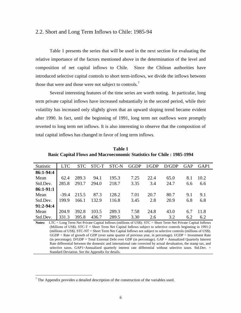
2.2. Short and Long Term Inflows to Chile: 1985-94

Table 1 presents the series that will be used in the next section for evaluating the

relative importance of the factors mentioned above in the determination of the level and

composition of net capital inflows to Chile. Since the Chilean authorities have

introduced selective capital controls to short term-inflows, we divide the inflows between

those that were and those were not subject to controls.7

Several interesting features of the time series are worth noting. In particular, long

term private capital inflows have increased substantially in the second period, while their

volatility has increased only slightly given that an upward sloping trend became evident

after 1990. In fact, until the beginning of 1991, long term net outflows were promptly

reverted to long term net inflows. It is also interesting to observe that the composition of

total capital inflows has changed in favor of long term inflows.

Table 1Basic Capital Flows and Macroeconomic Statistics for Chile : 1985-1994

Statistic LTC STC STC-T STC-N GGDP I/GDP D/GDP GAP GAP186:1-94:4MeanStd.Dev.86:1-91:1MeanStd.Dev.91:2-94:4MeanStd.Dev.

62.4285.8

-39.4199.9

204.9331.3

289.3293.7

215.5166.1

392.8395.8

94.1294.0

87.3132.9

103.5436.7

195.3218.7

128.2116.8

289.3289.5

7.253.35

7.013.45

7.583.30

22.4 3.4

20.7 2.8

24.8 2.6

65.024.7

80.720.9

43.0 3.2

8.16.6

9.16.8

6.76.2

10.2 6.6

9.1 6.8

11.8 6.2

Notes: LTC = Long Term Net Private Capital Inflows (millions of US$). STC = Short Term Net Private Capital Inflows(Millions of US$). STC-T = Short Term Net Capital Inflows subject to selective controls beginning in 1991:2(millions of US$). STC-NT = Short Term Net Capital Inflows not subject to selective controls (millions of US$).GGDP = Rate of growth of GDP (over same quarter of previous year, in percentage). I/GDP = Investment Rate(in percentage). D/GDP = Total External Debt over GDP (in percentage). GAP = Annualized Quarterly InterestRate differential between the domestic and international rate corrected by actual devaluation, the stamp tax, andselective taxes. GAP1=Annualized quarterly interest rate differential without selective taxes. Std.Dev. =Standard Deviation. See the Appendix for details.

7 The Appendix provides a detailed description of the construction of the variables used.

7

Total short term inflows have almost doubled, but at the expense of more than

doubling their volatility. A more interesting comparison arises when separating the short

term capital flows between those that are subject to the reserve requirement from those

that are independent of such control. The average volume of flows subject to controls has

increased by only 12% while their volatility has increased almost four times. On the

other hand, the level and volatility of those short term inflows not subject to controls have

almost tripled. As a matter of fact, the share of capital flows subject to controls in total

short term inflows has decreased substantially, from about 40% until the beginning of

1991 to 26% (on average) in the second period.

The time series behavior of both long term and short term capital inflows is

consistent with our expectations. In the case of long term capital inflows, we can see two

completely different “regimes”. During the first “regime” (1984-1989), net long term

capital inflows were on average negative and close to zero despite the strong positive

performance observed in the main domestic economic variables (strong output growth;

systematic increases in the investment rate and exports; and declines in inflation,

unemployment, the current account deficit and the external debt to output ratio) since

1983. Conversely, in the second “regime” (1990-1994), long term capital inflows have

been significantly positive with a strong upward slope, which is consistent with the

positive evolution of domestic structural economic variables.

A rationale for explaining this change in the behavior of long term flows can be

found in the positive way in which the international community has perceived Chile’s

successful transition to democracy and the renewed commitment of the country to sound

macroeconomic policies after 1990.

On the other hand, the fact that short term capital inflows not subject to a reserve

requirement increased on average much more than those subject to capital controls,

implying a significant change in the composition of short term capital inflows, may be

understood as a response to the introduction of reserve requirements in Chile.

In looking at the fundamentals, we observe that, while the investment rate has

been steadily increasing and the rate of growth of the economy has remained basically

stable, the debt-output ratio has suffered a dramatic decrease. The interest rate

8

differential increased slightly in the second period. Of course, this differential is even

wider if we do not include the several policy measures introduced by the Chilean

authorities to prevent a larger gap in favor of the domestic interest rate (the extension of

the stamp tax to foreign credit, the implementation of and subsequent modifications in the

reserve requirement, and the changes in the exchange rate policy).

Among other results, this brief look at the evidence suggests that it may be

misleading to analyze the determinants of long and short term inflows with a unique

stable representation for the whole sample period. In particular, it is important to analyze

the determinants of short term inflows considering the important differences that are

found among those that are and those are not subject to controls.

In order to account for these differences, it is necessary to utilize an econometric

technique that may be able to endogenously determine whether the realizations of a given

series correspond to the same stochastic process or if they come from different regimes. It

is also important to articulate the nature of these regimes as precisely as possible. The

following section briefly describes the estimation techniques used in the paper.

3. The Estimation Technique

The striking differences between the series in different periods points to the

importance of determining whether their changing behavior over time is attributable to

extreme realizations of a unique and stable stochastic process or to changes in the way the

series react to their fundamentals. In the first case, modeling the process would require a

careful consideration of the distributional assumptions employed; in the latter, one would

need to describe the characteristics of the transition from one regime to the other.

In order to select the econometric technique to be used in the next section, it is

important to identify the characteristics of the data-generating processes of the variables

we will use in our analysis.

Traditional Dickey-Fuller type tests do not reject the null hypothesis of unit root

for long term capital inflows, short term total private capital inflows, and (marginally) for

short term inflows subject and not subject to taxes. However, as Zivot and Andrews

9

(1992) show, tests of this type lack power when the series are characterized by stationary

processes with structural breaks. Tests of this type suggest a structural break for all

series.8 It must be recalled that all of these tests rely on univariate specifications; thus it

is still possible to obtain a stable representation for the series or at least to rule out some

of the breaks once additional information is included.

It is important, therefore, to use an econometric technique that allows the data to

discriminate between the presence of one or more regimes and, if possible, to determine

their sources. As a special case, it is still possible to obtain a unique stable relationship

between the differently defined private capital inflows and their determinants. In this

case, the technique should be flexible enough to allow consistent estimation with a full

sample and constant parameters.

Traditional techniques in these cases tend to use diverse specifications for

different periods. In doing so, however, it is implicitly assumed that the econometrician

has full knowledge of the precise moment and nature of the break. This methodology is

not advisable for several reasons: the econometrician may not know the precise moment

at which the regime switch takes place, nor may know whether the nature of the change is

temporary or permanent; even if the econometrician knows the nature of the change in

regime and the date at which it occurs, the sample size available makes it very difficult to

compute reasonable estimates for each period.

Labán and Larraín (1994) and Valdés and Soto (1996) have estimated simple

models to analyze the determinants of short and long term inflows to the Chilean

economy. In particular, Labán and Larraín (1994) conclude that the factors explaining the

behavior of short term private capital inflows to Chile since the mid-1980s are quite

different from those relevant to the evolution of medium and long term inflows. Their

results also show that short term inflows respond basically to interest rate arbitrage

opportunities --a combination of internal and external factors-- and to the decline in country

risk, proxied in their paper by the reduction in the foreign debt to GDP ratio. However,

8 This is evident particularly in the case of long term inflows. Sequential F tests for change in trend wereperformed and breaks were detected in 1990 and by the end of 1991 at conventional significance levels. Inthe case of short term flows, there is no perceivable modification in their level or the trend, while higher-order moments (particularly the variance) changed at the beginning of 1991.

10

they also conclude that the sharp increase in medium and long term private capital inflows

since the late 1980s appears to have been mainly a result of favorable domestic political and

economic changes. Of these changes, the most significant are the reduction of the debt

overhang, the better prospects of future economic growth (captured by a higher ratio of

investment to GDP) and the return to democracy. These have been translated, following

their argument, into a reduction of the premium that foreign investors require to invest in

Chilean long term securities. Their results also show that medium and long term capital

have not been sensitive to the interest rate differential or to the introduction and successive

modifications of the reserve requirements for foreign credits in effect in Chile since mid-

1991.

In the present paper we improve the structure of the model and the definition of

variables used by Labán and Larraín (1994), in an attempt to overcome certain

shortcomings apparent in the earlier paper. In particular, the econometric technique

utilized is too simple and the definition of medium and long term capital inflows considered

only some public sector flows. Due to limitations on data availability, they used Chapter

XIV flows as a proxy for total short term private capital inflows; these were precisely one of

the sources of short term capital inflows targeted by the selective capital controls

introduced.9 They also did not isolate the impact of these controls and of other policy

measures implemented, given that these were introduced in the definition of the interest rate

gap, in this way requiring a unique parameter to account for all of its components.

Valdés and Soto (1996) try to measure the impact that selective capital controls may

have had on the behavior of short term capital inflows. They conclude that the introduction

of selective controls to capital inflows did not have a statistically significant impact on

total short term inflows. In fact, they found a positive sign associated with the coefficient

of the implicit tax on short term inflows. Their data, however, are subject to the same

problems as the data set used by Labán and Larraín (1994), since some of the series they

consider include capital flows related to both the private and public sectors and they do not

9 The fact that these flows were negatively affected by the introduction and modifications of the reserverequirements does not necessarily imply that all short term private capital inflows reacted in the same way.Thus it may well be the case, that after the introduction of the “selective” capital controls there is a substitutioneffect from those short term capital inflows that are subject to controls to those that are not subject to controls.Therefore, these controls may have an ambiguous impact on overall short term capital flows.

11

differentiate between inflows that are and are not subject to controls. Other important

econometric problems are evident in their specification. In particular, the saturation ratio

of their short term inflows equation is very high (in excess of 33%), considering that they

have only 33 observations. The small sample size in conjunction with high collinearity

may be partially responsible for their results.10

A more serious problem evident in the specifications used in both papers is that

they do not consider that the dynamic properties of some capital inflows may be subject to

different regimes. In that case several problems may arise, among which are: i) full

sample estimation, not allowing for these changes, may lead to unreliable results and

unstable parameters; and ii) the way in which a set of variables (such as selective taxes)

affects capital inflows is non-trivial and may vary between regimes.

Given the arguments discussed above, Chumacero, Labán and Larraín (1996)

estimated Hamilton’s (1994) Markov Switching Regimes Models in order to assess

whether there is statistical evidence that favors the introduction of two different regimes

while modeling the determinants of short and long term private capital inflows. They

show that in most cases a unique stable representation for both short and long term

inflows is strongly rejected by the data and they proceed to estimate the characteristics of

the series when switching regimes are allowed. One problem that Chumacero et. al.

encountered is that the implicit tax series constructed by Valdés and Soto (1996) is highly

collinear with the interest rate differential. Therefore, their numerically intensive Markov

Switching Regimes Model was badly conditioned.

This paper uses several of the findings of Chumacero, et. al. (1996), but uses a

different estimation technique that is able to endogenously determine whether there are

different regimes in the sample period and, if so, what the nature of each regime is. A

brief description of the estimation technique, referred to as a threshold process, follows.

The technique consists of the estimation of a special case of non linear models in

which a particular variable may adopt a certain law of motion depending on whether or

10 The conditioning number of their equation exceeds 14, thus signaling an important problem ofcollinearity.

12

not an observation has passed a certain threshold. More formally, a two-regime threshold

process takes the form:

( ) ( )y x I q x I qt t t t t t= ′ ≤ + ′ > +1 2, ,α γ β γ ε (1)

where ( )I ⋅ denotes the indicator function, qt is a known function of the data, and γ is the

threshold parameter. Thus the parameters α is the vector of slope parameters when

qt ≤ γ , and β is the vector of slope parameters when qt > γ . (1) can be expressed more

compactly as:

( )y xt t t= ′ +γ θ ε (2)

where ( )θ α β= ′ ′ ′, and ( )x

x q

x qt

t t

t t

γγγ

=≤>

1

2

,

,

if

if .

Thus the problem faced in the estimation of (2) is not only to obtain estimates of

the vector of slope parameters but also of the threshold parameter. Under the additional

assumption that εt is normal, least squares estimation is equivalent to maximum

likelihood. Thus for a given value of γ, the LS estimate of θ , denoted by �θ is

( ) ( ) ( ) ( )�θ γ γ γ γ= ′

=

−

=∑ ∑x x x yt tt

n

t tt

n

1

1

1

(3)

with residuals ( ) ( ) ( )� �ε γ γ θ γt t ty x= − ′ and residual variance.

( ) ( )σ γ ε γn tt

n

n2 2

1

1==

∑ � (4)

Thus, the estimate of γ is the value that minimizes: ( )� argmin�γ σ γ= n2 , which can

be found by direct search. Remember that the estimate of γ depends ultimately on the

choice of qt that is observed by the econometrician.

Hansen (1996) presents a detailed explanation of the technique and derives the

asymptotic distribution of the estimates. An advantage of this specification is that

conventional likelihood ratio tests can be applied to test the null hypothesis of a unique

stable representation for the series against the alternative of a threshold process. This type

of specification can be viewed as a special case of the Markov Switching Regime Models

where the threshold variable replaces the transition matrix. From a computational

13

standpoint, a threshold process presents several attractive advantages given that it is not

as numerically intensive as the Markov switching model.

The following section reports the results of the estimation of this technique for

both long and short term inflows.

4. The Econometric Results

In order to apply the technique described in the previous section we followed

these steps:

• Run a full sample parsimonious regression for each series in order to determine the

variables that are to be included in the threshold process.

• For a given choice of the threshold variable we estimate the model and find the p-

value associated with the null of a unique stable representation.

• If a unique stable representation is rejected in favor of a threshold process, choose the

threshold variable that minimizes the sum of squares of the residuals.

• Reduce the threshold model to a parsimonious representation.

4.1. Long Term Inflows

Table 2 presents the full sample equation for long term capitals. Consistent with

the results of Labán and Larraín (1994) and Chumacero et. al. (1996), only structural

variables such as the investment rate and external debt-output ratio are significant, while

short term arbitrage conditions are not. As expected, important positive auto-correlation

is present in the data. Even though the long-term effect of the reduction of the debt-output

ratio is not statistically different from zero, an uncomfortable result from full sample

estimation is associated with the sign of the contemporaneous debt-output ratio.

Traditional tests suggest well behaved residuals but there is marginal evidence of

parameter instability, particularly associated with the coefficient of the investment rate

and departures from normality.

14

Table 2Determinants of Long Term Capital Inflows (Full Sample)

Variable Parameter Standard ErrorConstantLTC(-2)I/GDP(-2)D/GDPD/GDP(-2)

-1256.9050.568

53.15113.854

-10.833

349.6770.175

11.6505.6295.166

R²=0.649 SSR=1004274.8 DW=1.854 Q=0.913 JB=0.065 F=13.094Notes: See Table 1 for the definitions of the variables. Sample: 1986:1-1994:4. SSR=Sum of Squares of the

Residuals. Q=P-value of the Ljung and Box Chi² test for white noise (3 lags). JB=P-value of the Jarque andBera test for normality. F=F statistic. Standard errors of parameters are HAC.

In order to asses the existence of a threshold process we considered different

choices of the threshold variable qt recalling at this point that the only constraint is that it

belongs to the information set of the econometrician. Table 3 reports both the Sum of

Squares of the Residuals and bootstrap-calculated asymptotic p-value for the test of the

null hypothesis of linearity against the alternative of the particular threshold model. The

usage of bootstrapped p-values is recommendable in cases such as ours in which there is a

reduced sample size. Although other variables not present in the equation reported in

Table 2 were also included as possible candidates for the threshold variables, their results

are not as good in terms of sum of squared residuals as the ones reported in Table 3.

According to the results, there is strong evidence against a unique, stable, and

linear representation for long term private capital inflows. These results are consistent

with Chumacero et. al. (1996), who also find evidence of switching regimes in the series.

From Tables 2 and 3 we verify that the threshold model is able to halve the sum of

squares of the residuals of the original model. Of course, the cost is a reduction in degrees

of freedom. The preferred model suggests the threshold variable to be the

contemporaneous debt-output ratio. Given that this variable has shown a smoothly

decreasing trajectory, the threshold model endogenously determines to split the sample in

two periods.

15

Table 3Alternative Threshold Models for Long Term Capital Inflows

qt SSR P-valueLTC(-2)I/GDP(-2)D/GDPD/GDP(-2)

599565591671531958573789

0.3320.0710.0460.145

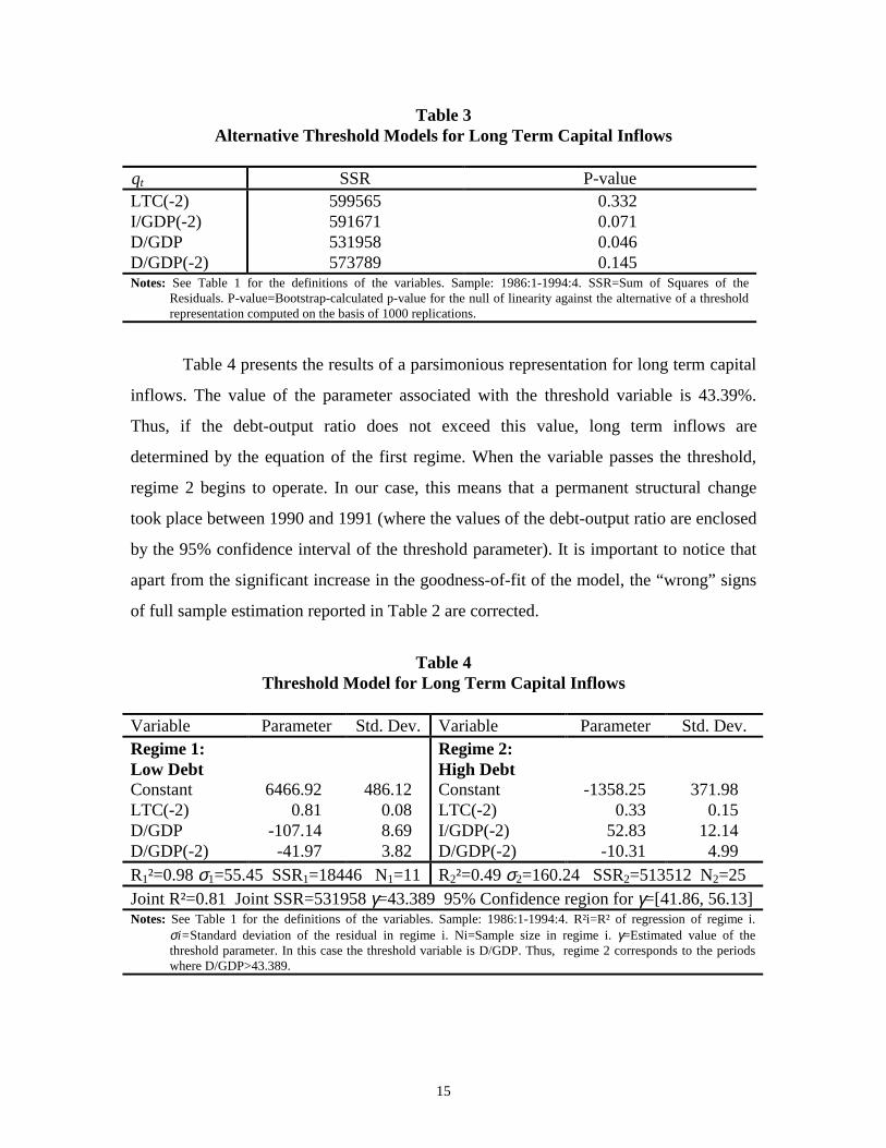
Notes: See Table 1 for the definitions of the variables. Sample: 1986:1-1994:4. SSR=Sum of Squares of theResiduals. P-value=Bootstrap-calculated p-value for the null of linearity against the alternative of a thresholdrepresentation computed on the basis of 1000 replications.

Table 4 presents the results of a parsimonious representation for long term capital

inflows. The value of the parameter associated with the threshold variable is 43.39%.

Thus, if the debt-output ratio does not exceed this value, long term inflows are

determined by the equation of the first regime. When the variable passes the threshold,

regime 2 begins to operate. In our case, this means that a permanent structural change

took place between 1990 and 1991 (where the values of the debt-output ratio are enclosed

by the 95% confidence interval of the threshold parameter). It is important to notice that

apart from the significant increase in the goodness-of-fit of the model, the “wrong” signs

of full sample estimation reported in Table 2 are corrected.

Table 4Threshold Model for Long Term Capital Inflows

Variable Parameter Std. Dev. Variable Parameter Std. Dev.Regime 1:Low DebtConstantLTC(-2)D/GDPD/GDP(-2)

6466.920.81

-107.14-41.97

486.120.088.693.82

Regime 2:High DebtConstantLTC(-2)I/GDP(-2)D/GDP(-2)

-1358.250.33

52.83-10.31

371.980.15

12.144.99

R1²=0.98 σ1=55.45 SSR1=18446 N1=11 R2²=0.49 σ2=160.24 SSR2=513512 N2=25Joint R²=0.81 Joint SSR=531958 γ=43.389 95% Confidence region for γ=[41.86, 56.13]Notes: See Table 1 for the definitions of the variables. Sample: 1986:1-1994:4. R²i=R² of regression of regime i.

σi= Standard deviation of the residual in regime i. Ni=Sample size in regime i. γ=Estimated value of thethreshold parameter. In this case the threshold variable is D/GDP. Thus, regime 2 corresponds to the periodswhere D/GDP>43.389.

16

Among other important differences between regimes, we see that the investment

rate is no longer statistically significant for determining long term inflows in the nineties,

whereas it performed a crucial role in the eighties. In the nineties, long term inflows are

more responsive to reductions in the debt-output ratio and are more persistent than before.

This may be due to the statistical properties of the investment rate after 1991, at which

point it has tended to stabilize, thus not providing additional information to foreign

investors. The fact that the threshold variable is the debt-output ratio, and given the

period in which it permanently switched to the first regime, suggests that there may be

other factors that triggered this change and of which this variable is a subset. This period

marks the return of democracy to Chile and the opening of the capital account.11 Another

very important feature is that the innovations in long term inflows were three times more

volatile in the eighties than in the nineties.

Both in the full sample estimation and in the threshold models, interest rate

arbitrage conditions and short term selective capital controls are not statistically relevant

in explaining the behavior of long run capital inflows to Chile since 1984.

4.2. Short Term Inflows Subject to Taxes

Table 5 presents the full sample equation for short term capital inflows subject to

controls. There we find that structural variables such as the investment rate or the

external debt-output ratio are not significant in the determination of this type of inflow.

We find, however, that short term arbitrage conditions, as well as the growth rate of the

economy, are statistically significant. One interpretation of the latter variable is that,

given the way in which the Central Bank of Chile carries out its monetary policy, an

increase in the growth rate of the economy may trigger a tight monetary policy and thus

an increase in the expected interest rate differential in the future, which would have a

positive impact on short term capital inflows subject to reserve requirement. After

deciding to bring capital into Chile and complying with the reserve requirement --

11 Labán and Larraín (1994) find a similar effect that they characterize as a dummy variable; in theirinterpretation this captured the return to democracy.

17

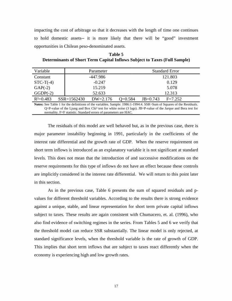
impacting the cost of arbitrage so that it decreases with the length of time one continues

to hold domestic assets-- it is more likely that there will be “good” investment

opportunities in Chilean peso-denominated assets.

Table 5Determinants of Short Term Capital Inflows Subject to Taxes (Full Sample)

Variable Parameter Standard ErrorConstantSTC-T(-4)GAP(-2)GGDP(-2)

-447.986-0.24715.21952.633

121.8030.1295.078

12.313R²=0.483 SSR=1562430 DW=2.176 Q=0.584 JB=0.743 F=7.252Notes: See Table 1 for the definitions of the variables. Sample: 1986:1-1994:4. SSR=Sum of Squares of the Residuals.

Q=P-value of the Ljung and Box Chi² test for white noise (3 lags). JB=P-value of the Jarque and Bera test fornormality. F=F statistic. Standard errors of parameters are HAC.

The residuals of this model are well behaved but, as in the previous case, there is

major parameter instability beginning in 1991, particularly in the coefficients of the

interest rate differential and the growth rate of GDP. When the reserve requirement on

short term inflows is introduced as an explanatory variable it is not significant at standard

levels. This does not mean that the introduction of and successive modifications on the

reserve requirements for this type of inflows do not have an effect because these controls

are implicitly considered in the interest rate differential. We will return to this point later

in this section.

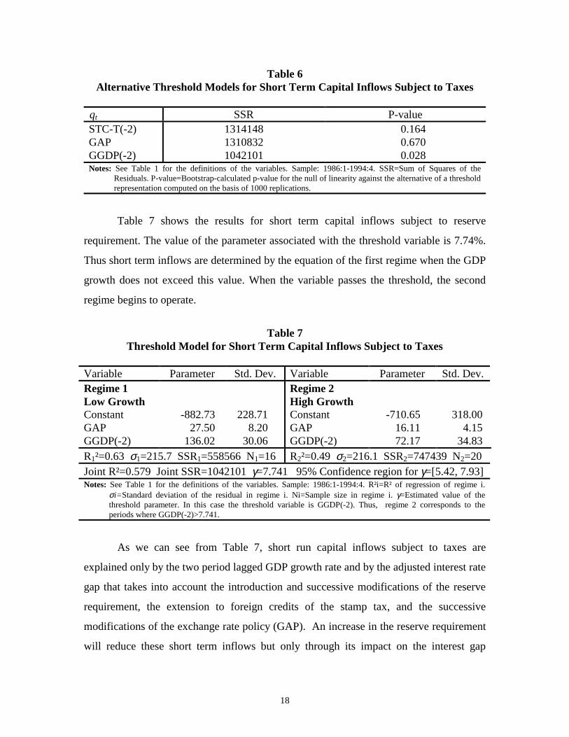
As in the previous case, Table 6 presents the sum of squared residuals and p-

values for different threshold variables. According to the results there is strong evidence

against a unique, stable, and linear representation for short term private capital inflows

subject to taxes. These results are again consistent with Chumacero, et. al. (1996), who

also find evidence of switching regimes in the series. From Tables 5 and 6 we verify that

the threshold model can reduce SSR substantially. The linear model is only rejected, at

standard significance levels, when the threshold variable is the rate of growth of GDP.

This implies that short term inflows that are subject to taxes react differently when the

economy is experiencing high and low growth rates.

18

Table 6Alternative Threshold Models for Short Term Capital Inflows Subject to Taxes

qt SSR P-valueSTC-T(-2)GAPGGDP(-2)

131414813108321042101

0.1640.6700.028

Notes: See Table 1 for the definitions of the variables. Sample: 1986:1-1994:4. SSR=Sum of Squares of theResiduals. P-value=Bootstrap-calculated p-value for the null of linearity against the alternative of a thresholdrepresentation computed on the basis of 1000 replications.

Table 7 shows the results for short term capital inflows subject to reserve

requirement. The value of the parameter associated with the threshold variable is 7.74%.

Thus short term inflows are determined by the equation of the first regime when the GDP

growth does not exceed this value. When the variable passes the threshold, the second

regime begins to operate.

Table 7Threshold Model for Short Term Capital Inflows Subject to Taxes

Variable Parameter Std. Dev. Variable Parameter Std. Dev.Regime 1Low GrowthConstantGAPGGDP(-2)

-882.7327.50

136.02

228.71 8.20 30.06

Regime 2High GrowthConstantGAPGGDP(-2)

-710.65 16.11 72.17

318.004.15

34.83R1²=0.63 σ1=215.7 SSR1=558566 N1=16 R2²=0.49 σ2=216.1 SSR2=747439 N2=20Joint R²=0.579 Joint SSR=1042101 γ=7.741 95% Confidence region for γ=[5.42, 7.93]Notes: See Table 1 for the definitions of the variables. Sample: 1986:1-1994:4. R²i=R² of regression of regime i.

σi= Standard deviation of the residual in regime i. Ni=Sample size in regime i. γ=Estimated value of thethreshold parameter. In this case the threshold variable is GGDP(-2). Thus, regime 2 corresponds to theperiods where GGDP(-2)>7.741.

As we can see from Table 7, short run capital inflows subject to taxes are

explained only by the two period lagged GDP growth rate and by the adjusted interest rate

gap that takes into account the introduction and successive modifications of the reserve

requirement, the extension to foreign credits of the stamp tax, and the successive

modifications of the exchange rate policy (GAP). An increase in the reserve requirement

will reduce these short term inflows but only through its impact on the interest gap

19

variable. Structural variables do not play any role in explaining the evolution of these

short term capital inflows.

An important question that can be addressed with this specification concerns the

effect that the introduction of selective capital controls had on the inflows that it targeted.

A brief description of the methodology used to answer this question follows.

Denoting by αi (for i=1, 2), the coefficients associated with the interest rate

differential (GAP), the impact effect that a change in the reserve requirement has on short

term inflows can be derived as:

∂∂

α ∂∂

STC T

TAX

GAP

TAXIt

ti

t

ti t

i

− ==∑ ,

1

2

(5)

where Ii,t denotes the indicator function for the threshold variable in period t, and

according to our definition of GAP:

( )∂∂

GAP

TAXT it

tt t= − −1 (6)

where T is the stamp tax, TAX is the tax equivalent of the reserve requirement on

selective inflows, and i is the nominal domestic interest rate. This impact effect is clearly

non constant and depends not only on the value of the stamp tax or the domestic interest

rate, but also on the overall performance of the economy. What is clear is that the impact

effect of a 1% increase in reserve requirements would be greater upon reducing this type

of inflows when the economy is in the low growth path, rather than when it is in the high

growth path. As a matter of fact, for the same levels of the interest rate and the stamp tax,

this impact effect would be 1.7 times greater in the low-growth path scenario (ratio of the

coefficients associated with GAP on Table 7). This is probably an upper bound, given

that it is more likely for the domestic interest rate to be higher in the high growth

scenario.

Given all the features described above, it is not surprising to find that the

composition of short term inflows has changed in favor of those flows that are not subject

to controls.

20

4.3. Short Term Inflows Not Subject to Taxes

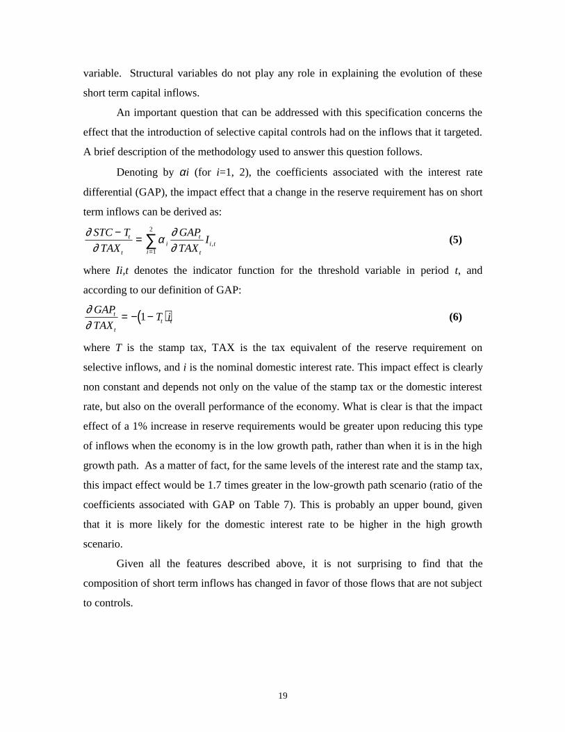
Table 8 presents the full sample equation for short term capital inflows not subject

to controls. Again we find that structural variables such as the investment rate, the

external debt-output ratio, or the growth rate of the economy are not significant in the

determination of this type of short term inflows. We find, however, that short term

arbitrage conditions and the reserve requirements are extremely important for this type of

short term inflows. It is important to mention that the relevant interest rate differential

here is GAP1 (that which does not consider the reserve requirements) given that these

inflows are not subject to taxes. The residuals of the model are well behaved, and there is

no evidence of significant parameter instability (although normality is rejected

marginally). As in the previous cases, Table 9 presents the sum of squared residuals and

p-values for different threshold variables.

According to these results there is no evidence against a unique, stable, and linear

representation for short term private capital inflows not subject to taxes. The results are

again consistent with Chumacero, et. al. (1996) who find evidence of a unique absorbing

regime. Thus the results of Table 8 show that a linear and stable relation exists. Notice

that in this specification there is a differentiated effected between the interest rate

differential (that excludes the implicit tax rate to short term inflows) and the tax rate

taken by itself. The coefficient associated with the first lag of the tax rate is positive and

statistically significant, implying a substitution effect from short term inflows that are

subject to taxes towards short term inflows that are not subject to taxes - an effect

reported in Chumacero et. al. (1996) and in Valdés and Soto (1996). Notice however,

that this short-run effect is completely offset in the third quarter (this effect was also

captured in Chumacero et. al. (1996), but not in Valdés and Soto (1996)).

21

Table 8Determinants of Short Term Capital Inflows Not Subject to Taxes (Full Sample)

Variable Parameter Standard ErrorConstantSTC-NT(-1)STC-NT(-2)STC-NT(-4)GAP1TAX(-1)TAX(-3)

162.600-0.487-0.2100.3025.311

42.615-41.128

31.5500.1030.1020.0802.7643.7613.211

R²=0.770 SSR=385274.4 DW=1.723 Q=0.123 JB=0.064 F=13.374Notes: See Table 1 for the definitions of the variables. Sample: 1986:2-1994:4. SSR=Sum of Squares of the

Residuals. Q=P-value of the Ljung and Box Chi² test for white noise (3 lags). JB=P-value of the Jarque andBera test for normality. F=F statistic. Standard errors of parameters are HAC.

Table 9Alternative Threshold Models for Short Term Capital Inflows

qt SSR P-valueSTC-NT(-1)GAP1T

341650360647343097

0.2160.7840.249

Notes: See Table 1 for the definitions of the variables. Sample: 1986:1-1994:4. SSR=Sum of Squares of theResiduals. P-value=Bootstrap-calculated p-value for the null of linearity against the alternative of a thresholdrepresentation computed on the basis of 1000 replications. d3(x)=x-x(-3).

Given that arbitrage is possible (at least in theory) between short term inflows that

are and are not subject to taxes, the relevant arbitrage conditions in this case is captured

by the coefficient associated with the contemporaneous gap between the domestic and the

international interest rate.

Given that the long run effect of an increase on reserve requirements deters

inflows subject to taxes and has no long run effect on inflows that are not subject to taxes,

its net effect is a reduction of total short term inflows and a permanent change in their

composition. This feature can not be captured with the aggregate series of short term

inflows, that lead to the “ineffectiveness” hypothesis advanced by Valdés and Soto

(1996).

22

5. Concluding Remarks

This paper presents a robust econometric methodology to analyze the

determinants of short and long term capital inflows to Chile during 1985-1994. Using

threshold processes we show that in most cases the determinants of these flows are

characterized by different regimes.

Long term inflows react to long run fundamentals such as the investment rate and

the external debt-output ratio and are not sensitive to short run arbitrage conditions. We

demonstrate that there has been a permanent structural break in the period 1990-91 that

coincides with economic factors such as the drastic reduction in the external debt-output

ratio and political aspects such as the return to democracy, among other important factors.

Since that period, long term inflows have been more persistent, more volatile and not

sensitive to the investment ratio.

We also show that in order to capture the dynamic properties of short term

inflows, it is necessary to divide them between those that are and those that are not

subject to selective controls.

Short term capital inflows that are subject to taxes have different determinants

depending on the business cycle. In particular, they react more strongly to arbitrage

conditions in low-growth scenarios. We also show that the effect of selective taxes on this

series is not constant. Given their distortionary nature they have a strong (and

asymmetric) influence on deterring the entrance of inflows subject to taxes. There is no

doubt that this fact helps to explain why their share in total short term inflows has been

dramatically reduced since the introduction of reserve requirements in Chile.

On the other hand, a unique stable representation for short term inflows that are

not subject to taxes is found in the data. It is also shown that changing the tax rate has no

long-term effect on this type of inflows.

In short, the introduction of reserve requirements on short term capital inflows has

had two main effects on these inflows. In the short-term, there is a clear substitution

23

effect away from capital inflows that are subject to taxes and into those that are not

subject to taxes. In the long run, the latter effect disappears and the deterrent effect on

inflows that are subject to taxes dominates. This analysis does not address the potential

efficiency losses of reserve requirements, but it clearly suggests that the case for the

ineffectiveness of capital controls may have been overstated.

24

Appendix: The Data

The definitions of the variables used in the model are:

• LTC = Quarterly Net Medium and Long Term Private Capital Inflows, include net

direct private investment (including secondary ADR), and medium and long term

foreign loans to the Chilean private banking and non banking sector.

• STC = Quarterly Net Total Short Term Private Capital Inflows, include short term

loans to the Chilean private banking and non banking sector (Chapter XIV), other net

private sector short term assets, changes in the stock of foreign currency deposits in

the Chilean banking system, and errors and omissions.

• STC-T = Quarterly Net Short Term Private Capital Inflows subject to selective capital

controls are short term loans to the Chilean private banking and non banking sector

(Chapter XIV), and (beginning in 1991:4) the changes in the stock of foreign currency

deposits in the Chilean banking system.

• STC-NT = Quarterly Net Short Term Private Capital Inflows not subject to capital

controls include other net private sector short term assets, changes in the stock of

foreign currency deposits in the Chilean banking system (until 1991 :3), and errors

and omissions.

• GAP = Annualized Quarterly Interest Rate Differential between domestic and the

“relevant” international interest rate. The domestic rate is the 90-day borrowing

market interest rate (i). The international “relevant” interest rate is the 90-day Dollar

LIBOR, until the second quarter of 1992; after that date, and considering the change

in the exchange rate regime, a weighted average of the 90-day nominal interest rates

of the US, Japan and Germany in US dollars (i* ) was used. The weighting factors

correspond to those in the currency basket that determine the central level of the

exchange rate band since that date. This gap also includes the stamp tax that was

extended to foreign credits since the second quarter of 1991 (T) and the tax equivalent

of the reserve requirement on selective short term capital inflows (TAX). Finally, the

observed exchange rate depreciation was utilized (e). Formally:

( ) ( )( ) ( )( )GAP T i t e i= − + − − + +1 1 1 1 1 * .* For the case of short term inflows not

25

subject to taxes the relevant interest rate differential is given by:

( )( ) ( )( )GAP T i e i1 1 1 1 1= − + − + + * .

*Note: In the GAP equation, t signifies TAX.The source for all data is the Central Bank of Chile.

26

References

Arrau, P. (1996). Política Financiera Internacional del Gobierno del Presidente PatricioAylwin. Manuscript.

Caballero, R. and V. Corbo. (1990). “The Effect of Real Exchange Rate Uncertainty onExports: Empirical Evidence”. The World Bank Economic Review.

Calvo, G., L. Leiderman and C. Reinhart. (1992). “Capital Inflows and Real ExchangeRate Appreciation in Latin America: The Role of External Factors”. IMF WorkingPaper. IMF.

Chumacero, R., R. Labán, and F. Larraín. (1996). What Determines Capital Inflows toChile?. Manuscript, Catholic University of Chile, July.

Corbo, V. and L. Hernández. (1993). The Macroeconomics of Capital Inflows: SomeRecent Experiences. Manuscript, Catholic University of Chile, July.

Culpeper, R. and Griffith-Jones. (1992). Rapid Return of Private Flows to Latin America:New Trends and New Policy Issues. Manuscript, ECLAC.

Hamilton, J. (1994). Time Series Analysis. Princeton University Press.

Hansen, B. (1996). Estimation of TAR Models. Manuscript, Boston College.

Hanson, J. (1992); “Opening the Capital Account: A Survey of Issues and Results”.World Bank Working Paper. The World Bank.

Krugman, P. (1987). “The Narrow Moving Band, the Dutch Disease, and the CompetitiveConsequences of Mrs. Thatcher: Notes on Trade in the Presence of DynamicScale Economies”. Journal of Development Economics.

Labán, R. and F. Larraín (1997). “Can a Liberalization of Capital Outflows Increase NetCapital Inflows?”. Forthcoming, Journal of International Money and Finance.

-------- and -------- (1996). The Return of Private Capital to Chile in the 1990s: Causes,Effects, and Policy Reactions. Manuscript, Catholic University of Chile.

-------- and -------- (1995). “Continuity, Change, and the Political Economy of Transitionin Chile” in R. Dornbusch and S. Edwards (editors), Stabilization, EconomicReform, and Growth. University of Chicago Press.

27

-------- and -------- (1994). What Drives Capital Inflows? Lessons from the RecentChilean Experience. Manuscript. Working Paper 168, Catholic University ofChile.

-------- and -------- (1993). “Twenty Years of Experience with Capital Mobility in Chile”in B. Bosworth, R. Dornbusch and R. Labán (editors). The Chilean Economy:Policy Lessons and Challenges. The Brookings Institution, Washington, D.C.

Larraín, F. and A. Velasco (1990). “Can Swaps Solve the Debt Crisis? Lessons from theChilean Experience”. Princeton Studies in International Finance No. 69.Princeton University.

Larraín, F. and R. Vergara. (1993). “Investment and Macroeconomic Adjustment: theCase of East Asia”. In L. Servén and A. Solimano (editors). From Adjustment toSustainable Growth: The Role of Capital Formation. The World Bank.

Morandé, F. (ed.). (1991). Movimiento de Capitales y Crisis Económica. ILADES-Georgetown University.

Salomon Brothers (1992). “Private Capital Flows to Latin America”. SovereignAssessment Group. New York.

Tobin, J. (1978). “A Proposal for International Monetary Reform”. Eastern EconomicJournal.

Tornell, A. (1990). “Real vs. Financial Investment: Can Tobin Taxes Eliminate theIrreversibility Distortion?”. Journal of Development Economics.

Valdés, S. (1994). “Financial Liberalization and the Capital Account: Chile 1974-84”. InG. Caprio, I. Atiyas, and J. Hanson (editors). Financial Reform: Theory andExperience. Cambridge University Press.

-------- and M. Soto. (1996). New Selective Capital Controls in Chile: Are they Effective.Manuscript, Catholic University of Chile, July.