BANKING THE POOR VIA SAVINGS ACCOUNTS:
EVIDENCE FROM A FIELD EXPERIMENT∗
Silvia Prina†
November 27, 2014
Abstract
In a setting with low penetration of bank accounts, I randomly gave accessto bank accounts with zero fees at local bank branches to a large sample offemale household heads in Nepal. The zero fees and physical proximity ofthe bank led to high take-up and usage rates compared to similar studiesin other settings. However, impact on income, aggregate expenditures,and assets are too imprecisely estimated to draw a conclusion. I do findreallocation of expenditures across categories (e.g. more spending on ed-ucation and meat and fish, and less on health and dowries), and higherability to cope with shocks. On qualitative outcomes, I find householdsreport that their overall financial situation has improved. The lack of aclear story on mechanisms, yet strong result on aggregate self-perceptionof financial wellbeing, is consistent with access to quality savings accountsleading to household improvements via multiple mechanisms.
JEL Codes: D14, O16, G21Keywords: savings accounts, financial access, transaction costs
∗I am grateful to Santosh Anagol, Manuela Angelucci, David Atkin, Carlos Chiapa, David Cling-ingsmith, Pascaline Dupas, Xavi Gine, Jessica Goldberg, Sue Helper, Dean Karlan, Dan Keniston,Cynthia Kinnan, Nicola Lacetera, David Lam, Dilip Mookherjee, Michael Porter, Nancy Qian, JonRobinson, Heather Royer, Scott Shane, Justin Sydnor, Chris Udry, Mark Votruba, Dean Yang, andnumerous conference participants and seminar participants at the 2011 and 2012 AEA Meetings,PacDev, MIEDC, NEUDC, Case Western Reserve University, CeRMi, ITAM, UC-Davis,UC-SantaCruz, University of Michigan, the World Bank, and Yale University for helpful comments and dis-cussions. I am grateful to GONESA for collaborating with me on this project, and Zach Kloos andAdam Parker for outstanding research assistance. I thank the IPA-Yale University Microsavings andPayments Innovation Initiative and the Weatherhead School of Management for funding. All errorsare my own.†Case Western Reserve University, Weatherhead School of Management, 11119 Bellflower Road,
room 273, Cleveland, OH 44106, United States. Fax: +1 216 368 5039. Phone: +1 216 368 0208.Email: [email protected]

1 Introduction
Saving promotes asset accumulation, helping to create a buffer against shocks and to
relax credit constraints, thus it may provide an important pathway out of poverty.
Although increasing evidence shows that the poor are willing and able to save, they do
so largely through informal mechanisms, such as storing cash at home, joining savings
clubs, and buying livestock and durable goods, which are illiquid and riskier than bank
accounts (Collins, Morduch, Rutherford, and Ruthven 2009; Karlan and Morduch
2010; Dupas and Robinson 2013b; Rutherford 2000). Unfortunately, the majority of
the world’s poor generally lack access to formal savings accounts or banking services
of any kind (Demirguc-Kunt and Klapper 2012).
This study examine the impact of offering a savings account with minimum trans-
actions costs, i.e. zero fees and high proximity to a bank-branch. Would poor house-
holds open and use such a savings account if given access to one? Would this access
help them to save, accumulating small sums into large sums? Would there be any
asset accumulation or welfare effects?
I address these questions via a randomized field experiment that considers a large
and diverse sample of households. Access to a simple bank account—with no opening,
maintenance or withdrawal fees—was randomly offered to a sample of 1,118 female
household heads in 19 slums in Nepal.1 The account that was offered operates through
local bank-branches. Through this experiment, I assess the causal impact of access
to the bank account on household saving behavior, asset accumulation, expenditures,
and income. I use two data sources: detailed household surveys at baseline and a
year after the start of the intervention, and bank administrative data.
My results show, first, that there is untapped demand for savings accounts without
opening, maintenance, or withdrawal fees, and proximity to local bank-branches: 84%
of the households that were offered the account opened one. Second, the poor do
save: 80% of the households that were offered the account used it frequently, making
1Female household head is defined here as the female member taking care of the household. Basedon this definition, 99% of the households living in the 19 slums were surveyed.
1
deposits of about 8% of their weekly income 0.8 times per week. Households slowly
accumulated small sums into large sums that they occasionally withdrew.
Despite the high take-up and usage rates, the impact on monetary assets and
total assets for treatment households compared to control households, a year after
the savings accounts were offered, is too imprecisely estimated to draw a conclusion.
Likewise, the aggregate expenditures measure is too noisy to detect a statistically
significant impact. Nevertheless, the treatment had a positive and statistically sig-
nificant effect on households’ expenditures on education, meat and fish consumption,
and festivals and ceremonies, and a negative effect on other items. Thus, it appears
that treatment households might have re-allocated their expenditures across items.
Such explanation would be consistent with the account holders’ withdrawal reasons
(from the bank administrative data), as well as with the reasons treatment households
reported they save in the account. Finally, financial access appear to have somewhat
improved the household’s self-reported financial situation.
Overall, my findings show that, if given access to a basic savings account with
minimum transaction costs, poor households do use it with high frequency. While
I cannot find a statistically significant effects on assets, access to a savings account
seems to help poor households to manage their resources better, changing their ex-
penditures across categories, although not in aggregate levels, and to report that their
overall financial situation has improved.
This study contributes to a better understanding of the characteristics that poor
households may value in a formal savings account and that may help explain take-up
and usage. The take-up and, especially, usage rates of the savings account offered
in this study are much higher than the ones found in other studies. A comparison
of the account features of the savings account considered in this study with those
offered in other interventions suggests that poor households appear to value a savings
product that is associated with low transaction costs in the form of proximity to a
local bank-branch and no fees, and that is offered by a trusted banking institution.
Distance from a bank-branch has been proposed as a reason for low usage of a savings
2

account (Brune, Gine, Goldberg, and Yang 2014). Also, as suggested by anecdotal
and survey evidence from Banerjee and Duflo (2011) and Dupas, Green, Keats, and
Robinson (forthcoming), high fees may discourage usage. Furthermore, lack of trust
in the banking institutions was reported as one of the main reasons people did not
begin saving in their account by Dupas et al. (forthcoming). Hence, consistent with
Karlan, Ratan, and Zinman (2014), decreasing transaction costs and improving trust
in banking institutions increases the effective usage of formal savings products by the
poor.
Another relevant result of this study is to show that, despite the lack of target-
based commitments, households are able to accumulate small sums into large sums
that are invested in targeted expenditure categories, such as education and food
consumption. An account without an explicit commitment might have advantages
and disadvantages for the poor. On the one hand, poor households might value such a
savings account as they can dip into their savings to address a shock, while permitting
them to safely store their money in good times. On the other hand, liquidity might be
an obstacle for accumulating savings. While few randomized experiments have shown
that commitment savings products help current or former bank clients and cash crop
farmers to save for a specific purpose, exercising their self-control early on (Ashraf,
Karlan, and Yin 2006b; Brune et al. 2014), this study shows that poor households
are able to save even with savings account without explicit commitments.
My paper contributes to the rapidly growing literature studying the impact of pro-
viding access to ordinary savings accounts,2 as well as commitment savings accounts,3
to different samples of individuals and households on a variety of outcomes.
This study is also linked to the non-experimental literature that shows that pro-
viding access to financial services to the poor appears to increase income and reduce
poverty (Aportela 1999; Burgess and Pande 2005; Bruhn and Love 2009).
2e.g., Ashraf, Karlan, and Yin 2006a; Brune et al. 2014; Cole, Sampson, and Zia 2011; Dupaset al. forthcoming; Dupas and Robinson, 2013a; Kast and Pomeranz 2014; McConnell 2012; andSchaner 2013.
3e.g., Ashraf et al. 2006b; Brune et al. 2014; Karlan and Linden 2014; Karlan, McConnell,Mullainathan, and Zinman 2012; Karlan and Zinman 2013; and Kast and Pomeranz 2014.
3

The following section describes the field experiment, the savings account, and the
data. Section 3 shows and discusses the results in terms of take-up and usage. Section
4 measures the impact of access to the savings account on assets, liabilities, and net
worth. Section 5 estimates the effects on household welfare, focusing on expenditures
and perceived financial situation. Finally, Section 6 concludes.
2 Background and Experimental Design
The field experiment took place in 19 slums in the area surrounding Pokhara, Nepal’s
second largest city. Some of these slums are right at the outskirts of the city, whereas
others are farther out in semi-rural and rural areas. This variation allowed me to
have a large and diverse sample of households.
2.1 Savings Institutions in Nepal
Formal financial access in Nepal is very limited: 26% of Nepalese households have
a bank account, according to the nationally representative “Access to Financial Ser-
vices Survey,” conducted in 2006 by the World Bank (Ferrari, Jaffrin, and Shrestha
2007). Access is concentrated in urban areas and among the wealthy. Thus, most
households typically save via microfinance institutions, savings and credit coopera-
tives, and Rotating Savings and Credit Associations (ROSCAs).4 Also, households
commonly have cash at home and save in the form of durable goods and livestock.
The main reasons reported in the nationally representative survey for not having a
bank account are transaction costs, especially distance from banking institutions, and
complicated deposit and withdrawal procedures. In addition, among those households
that reported having a bank account, usage is low: 54% of these households report
going to the bank less than once a month.5 Furthermore, having a bank account does
4A ROSCA is a savings group formed by individuals who decide to make regular cyclical contribu-tions to a fund in order to build together a pool of money, which then rotates among group members,being given as a lump sum to one member in each cycle.
5Going to the bank is a very good proxy of account usage because online banking is almostnonexistent in Nepal.
4

not necessarily mean that savings are deposited there. Only 37% of the households
that had an account and had savings in the previous year declared that they had
deposited money in the account. Moreover, banks typically charge high opening,
withdrawal, and maintenance fees and require a minimum balance.6
In the sample considered in this study, prior to the intervention, only 17% of the
households have a bank account, 35% less than in the national sample. This is con-
sistent with the fact that banks in Nepal tend to serve urban areas and the wealthy
(Ferrari et al. 2007). In fact, in the sample considered in this study, only some of
the slums are in urban areas and the average household earns $3 a day and has an
average size of 4-5 people. In line with the figures reported in the nationally represen-
tative survey, 18% of the sample were members of a ROSCA, and 54% belonged to a
microfinance institution or savings cooperative at baseline. Similarly to the nation-
ally representative sample, distance from banking institutions helps to explain why
households are unbanked. Indeed, there are no bank offices in the slums in which
the sample population lives, and the vast majority of bank branches are located in
the city center. Analysis of baseline data shows that an increase in transportation
costs as a fraction of monetary assets is negatively correlated with the probability of
having a bank account.
Considering loans, according to the Access to Financial Services Survey, 68%
of Nepalese households have an outstanding loan, whether from a formal financial
institution, informal provider, or both. Moreover, when considering all the sources
for loans, microfinance institutions and savings and credit cooperatives are by far the
largest providers (28%), followed by banks (24%) and family and friends (20%). In
the sample considered in this study, at baseline, the fraction of households with at
least one outstanding loan is 89%, 24% greater than in the national sample. This is
consistent with the low level of income and the high vulnerability to shocks of the
households in the sample. Furthermore, MFIs provide 34% of the total loans in the
6Minimum balance requirements vary from bank to bank and depend on the savings account type.Among the ten Nepalese banks with most branches, the most common minimum balance requirementis Rs. 500, equivalent to about $7, as Rs. 70 were approximately $1, during the intervention period.
5
sample, family and friends 24%, while banks only 4%.
Finally, Ferrari et al. (2007) state that an estimated 69% of foreign remittances
come through informal channels, usually family and friends, even among households
with a bank account. In the sample considered in the study, at baseline, one third
of the households who declared remittances as a source of income have a bank ac-
count. However, this does not necessarily imply that the account is used to receive
remittances.
2.2 The Savings Account
I worked in collaboration with GONESA, a non-governmental organization (NGO),
operating in 21 slums in the area of Pokhara, Nepal.7 In the early 1990s the NGO be-
gan to establish and manage one kindergarten center in each area. In 2008, GONESA
started operating as a bank and began offering formal savings accounts. The accounts
are very basic but have all the characteristics of any formal savings account.8 The
enrollment procedure is simple and account holders are provided with an easy-to-use
passbook savings account. Customers can make transactions at the local bank-branch
offices in the slums, which are open twice a week for three hours,9 or during regular
business hours at the bank’s main office, located in downtown Pokhara. Nevertheless,
this option is inconvenient because it requires customers to spend time and money
to travel to the city center. For safety considerations, the bank capped both deposits
and withdrawals made in the slums at Rs. 30,000. Thus, if an account holder wanted
to make a deposit or withdrawal above the cap, she had to go to the bank main office.
Nevertheless, nearly all transactions’ amounts were below the cap.10 Only 1% of the
21,450 transactions (i.e. withdrawals plus deposits), 13% of the 1,588 withdrawals,
7Two of the 21 slums were used to pilot the savings account. The field experiment analyzed inthis study was then conducted in the remaining 19 slums.
8The product offered by GONESA in this field experiment is the result of focus groups, productdesign, and pilot testing that I conducted jointly with the NGO.
9The established weekdays and business hours of each bank-branch office were publicly announcedat the start of the intervention and did not change.
10In the one-year period considered in this study, according to the bank administrative data, onlythree withdrawals and one deposit were above the cap (and took place at the bank’s main office).
6
and 18 of the 19,862 deposits made in the first year of operations took place in the
bank’s main office.
The bank does not charge any opening, maintenance, or withdrawal fees and pays
a 6% nominal yearly interest (inflation is above 10% in Nepal11), similar to the average
alternative available in the Nepalese market (Nepal Rastra Bank, 2011). In addition,
the savings accounts have no minimum balance requirement.12 Finally, the savings
account operates without any commitment to save a given amount or to save for a
specific purpose.
2.3 Experimental Design and Data
Before the introduction of the savings accounts, a baseline survey was conducted
in May 2010 in each slum. All households with a female head ages of 18-55 were
surveyed and the female household head was interviewed.13 This survey collected
information on household composition, education, income, income shocks, monetary
and non-monetary asset ownership, borrowing, and expenditures on durables and
non-durables. In total, 1,236 households were surveyed at baseline.
After completion of the baseline survey, GONESA bank progressively began op-
erating in the 19 slums between the last two weeks of May and the first week of June
2010, as follows. A pre-announced public meeting was held in each slum. Anybody
in the village who wanted to attend the meeting could attend.14 At this meeting,
participants were told (1) about the benefits of savings; (2) that GONESA bank was
about to launch a savings account; (3) the characteristics of the savings account; (4)
what the savings account could help them with and how they could use it; and (5)
that the savings account would only be initially offered to half of the households via
a public lottery. The short public talk was given by an employee of the bank with
11The International Monetary Fund Country Report for Nepal (2011) indicates a 10.5% rate ofinflation during the intervention period.
12The account’s conditions were guaranteed for as long as the participants chose to have an accountopen; in other words, the bank did not impose any time limit.
13The same respondent interviewed at baseline was interviewed at endline.14Attendance did not increase one’s probability of being offered an account.
7

the support of a poster and was followed by a short session of questions and answers.
The main aim of the session was to provide some kind of financial literacy on the
benefits of savings and savings accounts to the entire sample so that the effect of
the intervention would be mainly caused by the offer of the accounts.15 Then, sepa-
rate public lotteries were held in each slum to randomly assign the female household
heads to either the treatment group or the control group. There was no stratification
beyond village.16 Moreover, the number of individuals within each slum who would
have been offered the account was set for each public lottery. In each slum, every
female household head interviewed at baseline was entered in the lottery. Half of the
women in each slum were assigned, through a public lottery, to the treatment, the
other half to the control group.17
In total, 567 women were randomly assigned to the treatment group and were
offered the option of opening a savings account at the local bank-branch office;18 the
rest were assigned to the control group and were not given this option, but were not
barred from opening a savings account at another institution.19 Treatment households
could open the account on the first and subsequent days in which the bank was opened
in the slums, usually one to five days after the lottery.20 In order to open an account
a person needed to stand in line twice on two separate days: one day to have a picture
taken and to fill in an application, and a second day to receive the material related
to the account (account number, passbook, etc.).
A year after the beginning of the intervention, in June 2011, the endline survey was
15Only one public session was held in each slum. There were no individual marketing sessions.16GONESA required that the random assignment into treatment and control groups be done pub-
licly with balls in an urn, making stratification based on occupation or income infeasible.17If in a village there was an odd number of women, the 50% + 1 woman was assigned to the
treatment group.18The offer did not have a deadline.19Only 12% of the control households who declared not to have an account in the baseline survey,
reported to have one in the endline survey. Similarly, 11% of the treatment households who declarednot to have an account at baseline, reported to have one (aside from the account offered in the fieldexperiment) in the endline survey.
20The vast majority of account holders opened the account within the first month (22%, 45%,17% and 16% of the account holders opened the account in the first, second, third, and fourth week,respectively).
8

conducted. In addition to the modules contained in the baseline survey, information
on household expenditures and networks was also collected. The survey included
questions specifically addressed to the treated group that were aimed at understanding
the role played by supply and demand factors in explaining take-up and usage of the
account. Of the 1,236 households interviewed at baseline, 91% (i.e., 1,118) were found
and surveyed in the endline survey.21 Attrition for completing the endline survey does
not differ statistically between treatment and control households and is not correlated
with observables, as shown in the Appendix Table A1. Hence, performing the analysis
on the restricted sample for which there is endline data should not bias the estimates
of the treatment effect.
Finally, for the analysis presented in this paper, I also use GONESA bank’s ad-
ministrative data on savings account usage. These data include date, location (local
bank-branch office or main office), and amount of every deposit and withdrawal, as
well as the withdrawal reason, for all of the treatment accounts.22
2.4 Sample Characteristics and Balance Check
My sample comprised households whose female heads were, on average, 37 years old
and had less than three years of schooling (see Table 1A). Roughly 90% of respondents
were married or living with their partner. The average household size at baseline was
4-5 people, two of whom were children.
Weekly household income at baseline averaged Rs. 1,687 (equivalent to about $24,
as Rs. 70 were approximately $1 during the intervention period) although there is
considerable variation. Households earned their income from varied sources: working
as an agricultural or construction worker, collecting sand and stones, selling agri-
cultural products, raising livestock and poultry, running a small shop, working as a
driver or helper, making and selling wool and garments, working as a teacher, receiv-
21Considering treatment and control groups separately, 91% and 90% of the households in eachgroup were found, respectively. Those households that could not be tracked had typically moved outof the area, with a minority leaving the country.
22Households were not required to provide the reason of their withdrawal to the bank employeemanaging the transaction. Provision of such information was optional.
9

ing remittances and pensions, and collecting rents. Only 17% of the households listed
an entrepreneurial activity as their primary source of income.23 Also, the majority
of households (84%) reported living in a house owned by a household member, and
78% reported owning the plot of land on which the house was built.
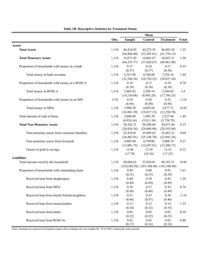
Table 1B shows households’ assets and liabilities at baseline. Total assets owned
by the average household had a value of more than Rs. 40,000. Monetary assets
accounted for 35% of total assets. Non-monetary assets—consumer durables, and
livestock and poultry24—accounted for the remaining 65%. As mentioned previously,
17% of the households were banked at baseline, 18% had money in a ROSCA, and
54% stored money in a microfinance institution (MFI). Households also typically had
more than one week’s worth of income stored as cash in their home.
Considering liabilities, as mentioned earlier, 89% of the households had at least
one outstanding loan. Most loans are taken from shopkeepers (40%), MFIs (38%),
family, friends, or neighbors (31%), and moneylenders (13%). Formal loans from
banks are rare, with only 5% of the sample reporting an outstanding loan borrowed
from a bank.
Summary statistics from Table 1B show a high level of participation by the sample
population in financial activities. However, most transactions are carried out with
informal partners, such as kin and friends, moneylenders, and shopkeepers rather
than with formal institutions like banks. This is consistent with previous literature
showing that the poor have a portfolio of financial transactions and relationships
(Banerjee, Duflo, Glennerster, and Kinnan forthcoming; Collins et al. 2009; Dupas
and Robinson 2013a; Rutherford 2000).
Finally, going back to Table 1A, the sample population seems highly vulnerable
to shocks; 41% of the households indicated having experienced a negative external
23I code as entrepreneurial activities: having a small shop, working as a driver, raising and sellinglivestock and poultry, selling agricultural products, making and selling wool and garments, andmaking and selling alcohol.
24Livestock and poultry include goats, pigs, baby cows/bulls/buffaloes, cows, bulls, buffaloes, chick-ens, and ducks.
10

income shock during the month previous to the baseline survey.25 Of the households,
52% coped with a shock using cash savings, 43% coped by borrowing ( 17% from
family and friends, 17% from a moneylender, and 9% from other sources). Only 1%
reported coping by cutting consumption or selling household possessions, possibly
suggesting that households have some ability to smooth consumption when facing a
negative shock.26
Overall, Tables 1A and 1B show that for the final sample considered for the
analysis (i.e., those 1,118 households that completed both the baseline survey and
the endline survey), treatment and control groups appear to be balanced along all
characteristics.27
3 Results: Take-Up and Usage
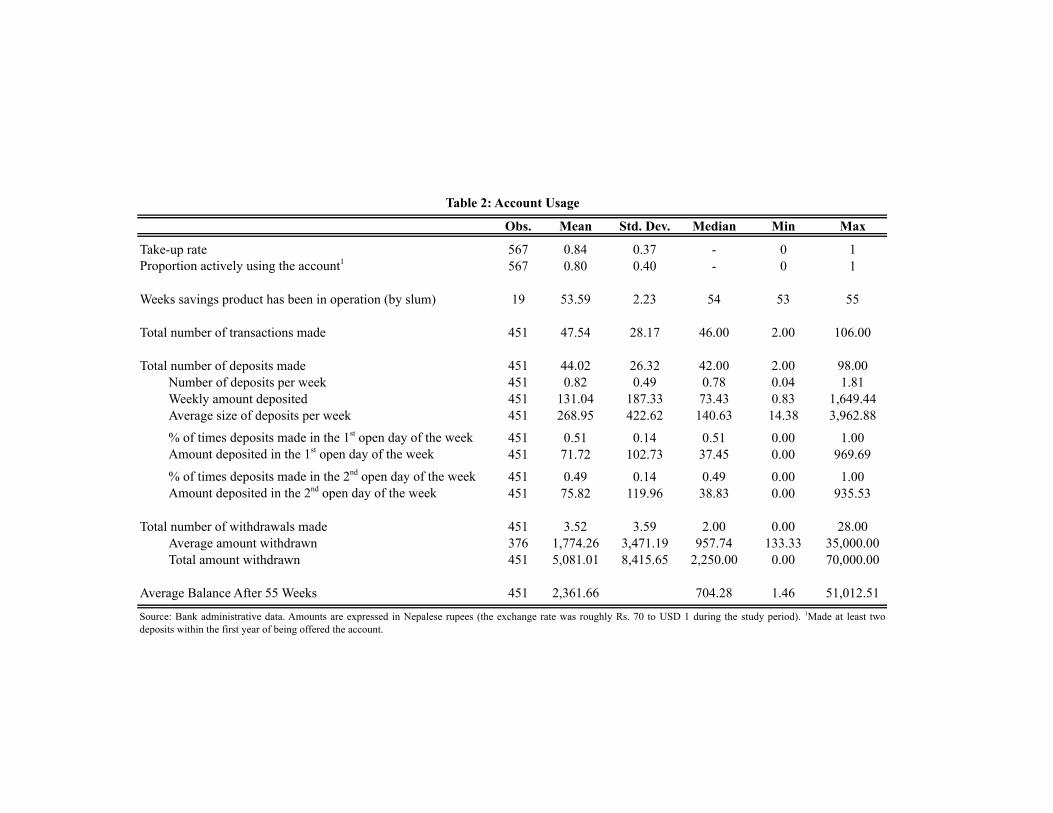
Of the 1,118 households included in the final sample, 567 were given the opportunity
to open a savings account. As shown in Table 2, 84% opened an account and 80%
used it actively, making at least two deposits within the first year of being offered the
account.28
To study the determinants of take-up and active use of the account I restrict
the sample to the treatment group, i.e. those individuals ever offered the account.29
Results, reported in the Appendix Table A2, show that take-up and active use of the
account are positively related to having a bank account at baseline, and negatively
related to earning income from an entrepreneurial activity. Moreover, belonging to
25Shocks include health shocks, lost job, livestock loss, broken/damaged/stolen goods or equipment,low demand for business, decrease in the wage rate, and death of a household member.
26An alternative explanation could be that shocks were small in economic terms.27The analysis carried out in this paper focuses on those 1,118 households that completed both
the baseline survey and the endline survey. However, the initial sample of 1,236 households thatcompleted the baseline survey is also balanced.
28For the original sample of 1,236 households surveyed at baseline, take-up and usage rates are notdifferent: 622 were given the opportunity to open a savings account, 82% took up the account, and77% used it actively.
29Take-up is a binary variable equal to 1 if the account was opened. Active use is a binary variableequal to 1 if the account holder made at least two deposits within the first year of being offered theaccount.
11

an MFI increases the probability of opening an account by 5%. None of the other
explanatory variables however, are statistically significant. This is not surprising given
that more than 80% of those offered an account opened one and used it actively.
The majority of the transactions that treated households made during the study
period were deposits. In fact, as shown in Table 2, account holders made an average
of 48 transactions: 44 deposits and 4 withdrawals. Forty-four deposits in a period
of 12 months is equivalent to 0.8 deposits per week. The average amount deposited
on a weekly basis was Rs. 131, roughly 8% of the average weekly household income
as reported in the baseline survey. The average weekly balance steadily increased
over the study period, reaching, a year after the start of the intervention, Rs. 2,362
for the average account holder.30 Account holders did not demonstrate a significant
preference for making deposits either sooner or later in the week. Rather, deposits
were evenly distributed between the first and second day of the week in which the
bank was open in the village, and were of very similar amounts. Nevertheless, the fact
that the local bank branch is open on pre-established days and at predetermined times
could potentially cause some kind of “reminder effect” and help the account holders
develop some habit formation to save regularly.31 Similarly, the limited opening hours
might have acted as an implicit commitment for some households. While this could
be the case, households could make withdrawals during regular business hours, as
in any other bank, at the bank’s main office. In fact 13% of the withdrawals took
place in the banks main office. Moreover, treated households did not perceive to be
limited in their access to the bank. In fact, 70% of the account holders reported as
the account feature they values the most the ability to easily deposit and withdraw
any amount of money any time (see Appendix Table A3, Panel B).
Comparisons of savings account balances across time show that households differ
in savings behavior. Savings were accumulated at different rates by each household,
30Bank administrative data on the interest rate accrued in a year by each account show that, onaverage, account holders earned a yearly interest of Rs. 126.
31Previous research has shown that reminders, via text messages or self-help group meetings, havea positive effect on savings (Karlan et al. 2012; Kast, Meier, and Pomeranz 2011).
12

depending on the frequency and size of deposits. Moreover, although 17% of the
households with a bank account actively deposited money over the course of the year
without making a single withdrawal, the majority accumulated small sums into larger
sums that then were eventually withdrawn, in full or in part.
Households also had different savings motives. Bank administrative data showed
that the main reasons for withdrawing money were to pay for a health emergency
(17%), to buy food (17%), to repay a debt (17%), to pay for school fees and materials
(12%), and to pay for festival-related expenses (8%). Hence, the savings accumulated
in the account were reportedly used for both planned expenditures and unexpected
shocks. The average size of a withdrawal was Rs. 1,774, slightly more than a week’s
household income.
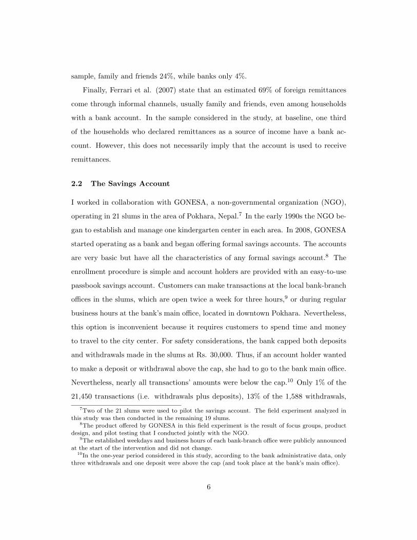
Figures 1 and 2 show the number of withdrawals made in any given week for the
five main withdrawal reasons listed above. Figure 1 considers withdrawals made for
education (school fees and school material) and festival-related expenditures. These
expenditures can be considered planned because the start of the school year and the
religious festivals happen on (arguably known) precise dates. In fact, withdrawals for
education-related expenditures spiked 49 weeks after the accounts had been offered
(i.e., during the week of April 18-24, which corresponds to the first week of school
for the Nepalese academic year 2011-2012). Similarly, withdrawals for festival-related
expenditures spiked at weeks 17, 22, 25, 35, 47, and 51 in correspondence with the
Teej festival, Dashain festival (which is considered the most important and lasts a
week), Tihar festival, Maghe Sankranti, New Year according to the Nepali calendar,
and Dumji festival, respectively.32
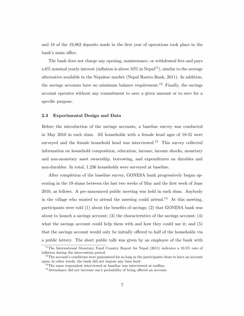
Figure 2 illustrates withdrawals made for health-related expenditures, to buy food
when income was low, and to repay a debt. There are not particular dates on which
withdrawals spike. This is partly explained by the fact that these are unplanned
expenditures incurred due to a negative shock to health or employment that occurred
32During the intervention period (i.e., May 2010-May 2011) the Teej festival happened on Septem-ber 11, Dashain festival from October 17-23, Tihar festival from November 4-8, Maghe Sankranti onJanuary 15, Nepali’s New Year on April 14, and Dumji festival on April 25.
13

randomly or that happened in the past, for which a loan was taken out. Hence,
households might be using the savings in the account as a buffer.
The administrative data are in line with the motives for saving as reported by the
households that had an account in the follow-up survey a year after the introduction
of the bank accounts (see Appendix Table A3, Panel A.) The top five reported reasons
for withdrawing the money saved in the account were health, consumption smoothing,
education, to pay for festival-related expenses, and to repay a debt.
The picture that emerges from the savings motives reported by the treated house-
holds in the sample tends to indicate that households might value access to a savings
account for different reasons than entrepreneurs do. When given access to the basic
savings account, households generally did not report using the money saved in the
account for microenterprise development, as entrepreneurs do (Dupas and Robinson
2013a).33 Nevertheless, they still reported using their savings to make productivity-
enhancing investments, such as education-related expenditures, and to smooth con-
sumption.
The bank administrative data also suggests that, given the high frequency of
deposits and the small size of weekly deposits, households seem to slowly accumulate
small sums into large sums. This saving behavior is very different from that observed
in entrepreneurs. In Dupas and Robinson (2013a), entrepreneurs in Kenya made few
and large deposits, equivalent to about 25% of their weekly income.
3.1 Discussion on Take-Up, Usage, and Account Features
A comparison of take-up and usage, and account features of the savings account con-
sidered in this study with those offered in similar interventions could shed some light
on the characteristics that the poor value in savings products. Table 3 reports, for each
of the studies that offered a savings account, the following information: the country
in which the field experiment took place; the setting (rural, semi-urban, urban); the
33Only 5% of the treated households withdrew to buy poultry or livestock, or to invest in theircurrent business. However, when restricting the sample to those households whose main source ofincome comes from an entrepreneurial activity, this percentage raises to 13%.
14

target population (banked/unbanked, male/female, entrepreneurs, farmers, salaried
workers, students, etc.); the type of account offered (ordinary, commitment, etc.);
whether the account charges opening fees and/or minimum balance fees; whether
there are withdrawal fees; whether there are deposit fees; the nominal interest rate
and inflation rate; the take-up rate; and the usage rate.34 Five studies offered an
ordinary savings account (Ashraf et al 2006a, Cole et al. 2011, Dupas and Robin-
son 2013a, Dupas et al. forthcoming, Schaner 2013), one study offered an ordinary
savings account with text message reminders (McConnell 2012), two studies offered
ordinary and commitment savings accounts (Brune et al. 2014, Kast and Pomeranz
2014), and four studies offered commitment accounts (Ashraf et al. 2006b, Karlan
and Linden 2014, Karlan et al. 2012, Karlan and Zinman 2013).
Compared to other studies that offered an ordinary savings account with no open-
ing or minimum balance fees, there is large variation in take-up rates. On the one
side, Dupas and Robinson (2013a) obtained an 87% take-up rate when offering the
option to open an account to a sample of microentrepreneurs in rural Kenya; Dupas
et al. (forthcoming) found a 62% take-up rate when offering the option to open an
account to a random subset of unbanked individuals in rural Kenya; and Schaner
(2013), who offered to 749 previously unbanked couples in rural Kenya both individ-
ual and joint savings account, obtained that all couples opened at least one account.35
On the other side, Ashraf et al. (2006a) found a 28% take-up rate when offering a
savings account to 346 existing or former clients of a rural bank in the Philippines;
McConnell (2012) obtained a 12% when offering a savings account to 1,601 market
vendors in Ghana, 39% of which were already are banked; and Cole, Sampson, and
Zia (2011) found a take-up rate of around 10% among unbanked households in rural
and urban Indonesia, despite the fact that a $3-$14 subsidy was provided for opening
an account.
34Not all this information was available for the studies reported. When the information was notavailable, it was noted with NR, as in not reported.
355% of the couples chose to open all three accounts offered (one of for each partner and a jointaccount).
15

Since the take-up rates of the ordinary savings accounts offered in Dupas and
Robinson (2013a), Dupas et al. (forthcoming), and Schaner (2013) are the most
similar to the one in my study (84%), I continue the comparison with these studies.
As mentioned earlier, 80% of treatment households in my study used the account
actively, making at least two deposits in a year.36 The usage rates in these other
three studies are much lower. In Dupas and Robinson (2013a), 41% of their treatment
entrepreneurs used the account actively (making at least one transaction within the
first six months), while in Dupas et al. (forthcoming) only 18% of the treatment
individuals used the account actively (making at least two deposits in a year), and
in Schaner (2013) 22% of the accounts were active, i.e. received at least one deposit
within the first six months.
These differences in usage rates could be due to many reasons including the differ-
ent contexts considered and differences in the savings products offered. First, diverse
savings behaviors and informal saving options available to the poor in Kenya and
Nepal might partly explain this variation in usage rates. Formal and informal savings
options in Kenya and Nepal however, are comparable in terms of features, costs, and
convenience. Moreover, previous literature has shown that the poor want to save and
do so using several savings mechanisms that are similar across countries (Collins et
al. 2009; Rutherford 2000).
A second explanation may be the lack of trust in banking institutions and their
service reliability. While trust, does not seem to be an issue in Nepal, it is in Kenya
where, among the three main reasons people do not use their bank accounts, are lack
of trust in banking institutions and unreliable service (Dupas et al. forthcoming).37 In
my sample, trust in the banking institution that offered the account was considered the
most valued account feature by only 9% of the users.38 This could also be explained
36When considering only the treated households (i.e. those that when offered an account decidedto open one) the percentage of active users is 95%.
37Part of the reason could be due to the fact that in Nepal insurance of deposits up to Rs. 200,000is mandatory for banks and financial institutions in order to safeguard savings of small depositors.
38Detailed percentages on the account features most valued are reported in Appendix Table A4,Panel B.
16

by the fact that households in my sample knew the GONESA since the 1990s, thus
it might have been easier for them to entrust their money with GONESA bank.
Third, rural versus semi-urban and urban settings, where the risk of theft of cash
kept at home might be higher might explain the variation in usage rates. Dupas
and Robinson (2013a), Dupas et al. (forthcoming), and Schaner (2013) consider a
rural setting, while the households considered in my sample live in rural, semi-urban,
and urban settings. Nevertheless, the bank administrative data do not show any
differences in usage rates when comparing frequency and amounts of deposits, and
frequency of withdrawals between households living in semi-urban and urban areas
compared to the ones living in rural areas.
Fourth, diverse occupations (e.g., entrepreneurs versus non-entrepreneurs) could
also explain such differences in usage rates. Nevertheless, the bank administrative
data do not show any differences in usage rates when comparing frequency and
amounts of deposits, and frequency of withdrawals between households involved in
entrepreneurial activities and the rest of the sample.39
Aside from the differences in the contexts considered, differences in the character-
istics of the savings products offered might also matter. A likely explanation for the
differences in usage rates may rely on the minimum transaction costs of the savings
product offered, due to proximity to local bank-branches and the lack of fees.
The account offered aimed at improving convenience by enabling customers to
make transactions, not only during business hours at the bank’s main office, but also
at the local bank-branch offices in the slums, opened twice a week for three hours.
Physical proximity to a local bank-branch seems to matter: 99% of total transactions
made by account users over the first year took place in the local bank-branches,
despite the fact that they were open only twice a week for three hours. Moreover,
as mentioned previously, 70% of the account holders reported as the account feature
they values the most the “ability to easily deposit and withdraw any amount of
39There is a difference in the average withdrawal size, which is Rs. 2,751 for households whose mainsource of income comes from an entrepreneurial activity and Rs. 1,578 for the rest of the sample.
17

money any time.” This is consistent with the finding that, at baseline, households
are less likely to be banked, the higher the cost of going to the bank.40 Similarly,
the 2006 World Bank survey indicates that most Nepalese households do not have or
use a bank account because of distance. Furthermore, Dupas and Robinson (2013a)
discuss that the low frequency of transactions and the high median deposit size, in
their sample, are consistent with the fact that, as the bank’s business hours were
inconvenient, individuals saved up for some time and then deposited larger sums,
instead of building up savings balances by depositing small amounts of money, as
in my sample. Hence, convenience appears to be an important factor in influencing
usage of a savings account.
Finally, lack of withdrawal fees may also be playing a role. Whereas in Dupas and
Robinson (2013a), Dupas et al. (forthcoming), and Schaner (2013), account opening
fees and minimum balance fees were waived, only in my study did withdrawal fees get
waived as well. In fact, Dupas et al. (forthcoming) report survey evidence suggesting
that one of the main reasons of low usage of bank accounts are expensive withdrawal
fees. Moreover, anecdotal evidence from Banerjee and Duflo (2011) emphasizes the
importance of high withdrawal fees in the poor’s decision not to use a savings account.
Overall, the high usage rates observed in this study might be explained partly by
trust in the banking institution and minimum transaction costs in the form of physical
proximity to a bank-branch and zero fees. This is consistent with the constraints that
may hinder the effective usage of savings products by the poor discussed by Karlan,
Ratan, and Zinman (2014) in their review of the empirical evidence on access to
savings accounts.
4 Results: Assets, Liabilities, and Net Worth
The high take-up and usage rates of the account that was offered suggest potential
effects on asset accumulation. In this section, I study the impact of access to a formal
40The cost of going to the bank is defined as the transportation cost, by bus, from each slum tothe center of Pokhara, where bank-branches are, as fraction of monetary assets.
18
savings account on household assets a year after the start of the randomized inter-
vention. The main outcome variables of interest are monetary assets, non-monetary
assets, and total assets. Monetary assets include cash at home; money in banks;
money in MFIs; money in ROSCAs; money kept for safekeeping by a friend, relative,
or employer; and, for the treated households only, money they report having in the
savings account they were offered by GONESA bank. Reported balances are highly
predictive of actual account balances. For more than 95% of the treated households
the reported balances are within a 5% difference of the actual balance they have in the
account. Non-monetary assets include consumer durables, and livestock and poultry.
Total assets include monetary and non-monetary assets. I also study the effect of
access to a savings account on liabilities and net worth (total assets minus liabilities).
In order to quantify the effects of the intervention, I estimate the average effect
of having been assigned to the treatment group, or intent-to-treat effect (ITT), on
each outcome variable Y a year after the launch of the savings account.41 I use the
following regression specification:
Yi,t = β0 + β1Ti + β2Yi,t−1 + β3Xi,t−1 + λv + εi,t (1)
where Ti is an indicator variable for assignment to the treatment group, Yi,t−1
is the baseline value of the outcome variable, Xi,t−1 is a vector of baseline charac-
teristics (age, years of education, and marital status of the account holder; number
of household members; baseline household income; and three dummies for the main
source of household income42), and εi is an error term for household i. I also include
41I do not analyze the average effect for those who actively used the account because, among thosewho opened an account, only 5% (26/477) did not actively use it.
42The three dummies for the main source of household income are: income from an entrepreneurialactivity, as salaried worker, and as casual worker. The omitted category is other sources of income.I coded as entrepreneurial activities: having a small shop, working as a driver, raising and sellinglivestock and poultry, selling agricultural products, making and selling wool and garments, andmaking and selling alcohol. I coded as salaried worker the following activities: government job,private job (full time), and teacher. I coded as casual worker the following activities: agriculturalworker, sand and stone collector, construction worker, bus fare collector, helper, and other part-time/temporary job. The omitted category is other sources of income, i.e. pension, rent, remittances,jewelry income, and other sources.
19

village fixed effects λv because the randomization was done within village. I report
the regression results both with and without controls and village fixed effects. The
coefficient of interest is β1, which estimates the intent-to-treat (ITT) effect.43
Table 4 presents the overall average effects of the savings account on monetary
assets (columns 1-2), non-monetary assets (columns 3-4), total assets (columns 5-6),
liabilities (columns 7-8), and net worth (columns 9-10). None of the intent-to-treat
coefficients is statistically significant. Measures of assets, liabilities and net worth are
inherently noisy and, consequently, the standard errors are large. Nevertheless, the
magnitude of the ITT estimate for monetary assets (1,982.18) is similar to the average
savings balance for the treatment group (calculated using the bank administrative
data). In fact, as shown in Table 2, those households in the treatment group that
opened an account and used it actively (80% of the treatment group, 451 out of
567), accumulated on average over the course of a year Rs. 2,362. Thus, the average
household in the treatment group accumulated on average Rs. 1,889 (2,362*0.8).
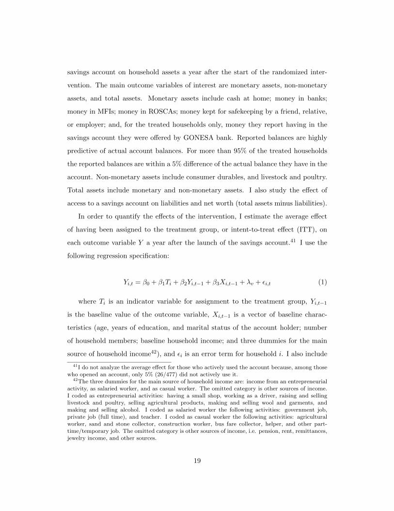
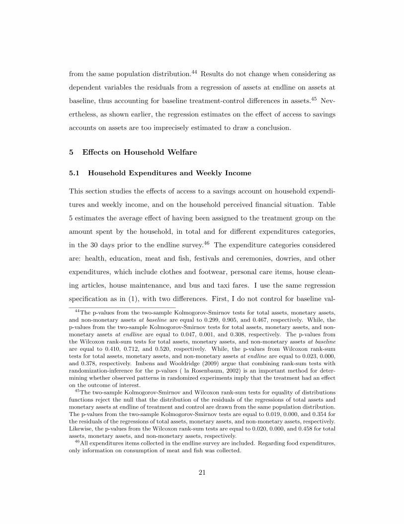
Moreover, Figure 3 shows the cumulative distribution functions (CDFs) of mon-
etary, non-monetary and total assets at baseline (Figure 3A) and at endline (Figure
3B) for the treatment (grey line) and control (dashed line) groups. At baseline, there
do not seem to be any sizeable differences for any asset category. A year after the
start of the intervention however, the monetary asset CDF for the treatment group
appears to the right of the one for the control group, indicating the positive effect of
getting access to a savings account on monetary assets. Similarly for total assets. I
calculated the p-values from the two-sample Kolmogorov-Smirnov and the Wilcoxon
rank-sum tests for equality of distributions functions for each asset category both at
baseline and at endline. The two-sample Kolmogorov-Smirnov and Wilcoxon rank-
sum tests for equality of distributions functions reject the null that the distribution
of total assets and monetary assets at endline of treatment and control are drawn
43Assuming that being offered the savings account does not have any other direct effect on savingsother than motivating an individual to use the account, it is possible to estimate the treatment-on-the-treated effect by dividing the ITT by the take-up rate ( β1
take-up rate).
20
from the same population distribution.44 Results do not change when considering as
dependent variables the residuals from a regression of assets at endline on assets at
baseline, thus accounting for baseline treatment-control differences in assets.45 Nev-
ertheless, as shown earlier, the regression estimates on the effect of access to savings
accounts on assets are too imprecisely estimated to draw a conclusion.
5 Effects on Household Welfare
5.1 Household Expenditures and Weekly Income
This section studies the effects of access to a savings account on household expendi-
tures and weekly income, and on the household perceived financial situation. Table
5 estimates the average effect of having been assigned to the treatment group on the
amount spent by the household, in total and for different expenditures categories,
in the 30 days prior to the endline survey.46 The expenditure categories considered
are: health, education, meat and fish, festivals and ceremonies, dowries, and other
expenditures, which include clothes and footwear, personal care items, house clean-
ing articles, house maintenance, and bus and taxi fares. I use the same regression
specification as in (1), with two differences. First, I do not control for baseline val-
44The p-values from the two-sample Kolmogorov-Smirnov tests for total assets, monetary assets,and non-monetary assets at baseline are equal to 0.299, 0.905, and 0.467, respectively. While, thep-values from the two-sample Kolmogorov-Smirnov tests for total assets, monetary assets, and non-monetary assets at endline are equal to 0.047, 0.001, and 0.308, respectively. The p-values fromthe Wilcoxon rank-sum tests for total assets, monetary assets, and non-monetary assets at baselineare equal to 0.410, 0.712, and 0.520, respectively. While, the p-values from Wilcoxon rank-sumtests for total assets, monetary assets, and non-monetary assets at endline are equal to 0.023, 0.000,and 0.378, respectively. Imbens and Wooldridge (2009) argue that combining rank-sum tests withrandomization-inference for the p-values ( la Rosenbaum, 2002) is an important method for deter-mining whether observed patterns in randomized experiments imply that the treatment had an effecton the outcome of interest.
45The two-sample Kolmogorov-Smirnov and Wilcoxon rank-sum tests for equality of distributionsfunctions reject the null that the distribution of the residuals of the regressions of total assets andmonetary assets at endline of treatment and control are drawn from the same population distribution.The p-values from the two-sample Kolmogorov-Smirnov tests are equal to 0.019, 0.000, and 0.354 forthe residuals of the regressions of total assets, monetary assets, and non-monetary assets, respectively.Likewise, the p-values from the Wilcoxon rank-sum tests are equal to 0.020, 0.000, and 0.458 for totalassets, monetary assets, and non-monetary assets, respectively.
46All expenditures items collected in the endline survey are included. Regarding food expenditures,only information on consumption of meat and fish was collected.
21

ues of expenditures, since information about household expenditure was not collected
at baseline. Second, I add as additional baseline controls the amount of liabilities,
having a bank account, belonging to an MFI, and belonging to a ROSCA.
Estimates show that the total household expenditures measure is too noisy to
detect a statistically significant impact. Nevertheless, financial access has a positive
and statistically significant effect on expenditures in education, meat and fish, and
festivals and ceremonies. Treatment households spend on average 20% more in edu-
cation and 15% more in meat and fish than control households. On the other side,
there appears to be a negative (not statistically significant) impact on expenditures
on health expenditures and dowries. Thus, it might be the case that treatment house-
holds might have re-allocated their expenditure across items. Such explanation would
be consistent with the account holders’ withdrawal reasons (from the bank admin-
istrative data), as well as with the reasons treatment households reported they save
in the account. In fact, as mentioned earlier, bank administrative data show, among
the main reasons for withdrawing money, to buy food (17%), to pay for school fees
and materials (12%), and to pay for festival-related expenses (8%). This is also in
line with the motives for saving as reported by the households that had an account
in the follow-up survey a year after the introduction of the bank accounts (Appendix
Table A3, Panel A).
As shown in Table 5, columns 5-6, access to a savings account had a positive
and statistically significant effect on treatment households’ expenditure on education.
Regression results reported in Table 6 restrict the sample to those households with
children 6-16 years of age. Estimates in columns 3-4 show that, restricting the sample
to those households with children of school age, the impact of access to a savings
account on the overall expenditures in education is greater. Furthermore, the endline
survey collected expenditures in education in four different subgroups: school fees,
textbooks, uniforms, and school supplies, such as pens and pencils. Regression results
reported in Table 6, columns 5-12, show higher investments in human capital for the
treatment group than for the control.
22
The increase in investment in human capital appears to be on the intensive margin,
not on the extensive margin. In fact, as columns 1-2 of Table 6 show, the treatment
group is not more likely than the control group to have at least one of their children
enrolled in school. This would be expected because an already high percentage of
households with children 6-16 years of age has at least one child in school (81%).
The estimated effects on the education-related expenditures are likely to be a lower
estimate of the actual effects. The peak in withdrawals for education expenditures,
as shown in Figure 1, was around the beginning of the school year, which happened
almost two months before the start of the of the endline survey.
Next, Table 7 analyzes the effect on household weekly income and exposure to
health shocks. When considering the full sample, there is no statistically significant
difference in weekly income for treatment and control households. Also, access to a
savings account does not appear to have reduced exposure to health risk. In fact,
23% of the treatment households and 22% of the control households were hit by a
health shock, and the difference is not statistically significant.
When restricting the sample to those households hit by a health shock in the last
30 days prior to the endline, the weekly income of households hit by a shock 30 days
prior to endline decreases for both treatment and control group. However, treatment
households suffer smaller reductions in income than control households: the weekly
income of the average treatment household is Rs. 1,325 higher than the one of the
average control household (Rs. 1,799), and this difference is statistically significant.
Moreover, the weekly income of the average control household hit by a shock is 40%
lower than the one of the average control household in the full sample (Rs. 1,799 versus
Rs. 3,012), while the weekly income of the average treatment household hit by a shock
is only 15% lower than the one of the average treatment household (Rs. 3,124 versus
Rs. 3,699). This evidence tends to suggest that households offered a savings account
do not suffer such large changes in weekly income when hit by a health shock during
the previous month as control households. This could be explained by treatment
households making other investments (e.g., more meat and fish), which may increase
23
the households’s “health capital,” causing members of treatment households to be
affected by a health shock less strongly than control households, and being able to
recover faster, thus missing less working days.47 Another possible explanation could
be that access to savings allows for more effective treatment, leading to faster recovery
for the same severity of illness. Furthermore, as columns 7-8, shows, while the effect
is not statistically significant, treatment households appear to spend less on health
expenditure than control households. Similarly, columns 9-10 show that treatment
households appear borrow less money when hit by a health shock, though, again, the
coefficient is not statistically significant. The lower health-related expenditure and
loans are consistent with the treatment group’s ability to recover faster from health
shocks than the control.
5.2 Overall Financial Situation
Table 8 presents the average effects of access to a savings account on the households’
self-assessed financial situations. The endline survey a year after the start of the
intervention contained three questions aimed at measuring the household’s perceived
financial situation. As shown in columns 1-2, households offered the savings account
are 9% more likely to describe their financial situation as “living comfortably” or
“having a little left for extras.” In addition, estimates from columns 3-4 indicate that
treatment households are also 7% more likely not to feel very or at all financially
stretched month to month. Access to a savings account, however, does not improve
households’ sense of financial security, as presented in columns 5-6. The fact that
treatment households do not feel more financially secure, while not feeling stretched
or having a little left for extras, might be consistent with the fact that, while access
to a savings account might have helped households manage their resources better, feel
more in control, and be better able to cope with health shocks, it did not improve their
overall financial situation. In fact, households assets and income did not increase.
47This finding is consistent with treatment households possibly eating a more varied diet whichincludes meat and fish (see Table 5, columns 7-8).
24

Finally, the last two columns of Table 8 report the ITT estimates for an overall
measure that aggregates the three outcomes of interest considered in columns 1-6. I
construct this index following Kling et al. (2007) and Karlan and Zinman (2010).
First, I standardize each of the three outcome variables into a z -score by subtracting
its control group mean and dividing by its standard deviation. Then, I combine
the three new outcome variables into one by taking the average of equally weighted
standardized components. Thus, the treatment effect for the summary index is an
estimate of the average effect on each outcome variable that composes the index, in
standard deviation units. Regression results reported in columns 7-8 show that access
to a savings account has a positive and statistically significant effect of 0.09 standard
deviation units on the “overall financial situation” index. Hence, access to a savings
account appears to have improved the household’s perceived financial situation.
6 Conclusion
The poor often lack access to formal financial services, such as savings accounts,
and have to adopt costly alternative strategies to save. Access to formal financial
services that enable saving and asset building might be important for low-income
households to smooth sudden income fluctuations due to negative shocks such as
medical emergencies. Savings can also provide capital to be invested in education.
I use a randomized field experiment and the combination of pre- and post-survey
data with bank administrative data to study the effects of access to a savings account
with minimum transaction costs, i.e. zero fees and physical proximity to a local bank-
branch, on household savings behavior and welfare. My study shows that there is high
demand for this type of savings accounts and that households regularly deposit small
amounts of money.
Despite the high take-up rate and usage rates, access to a savings account gen-
erates minor welfare effects. Impact on assets, aggregate expenditures, and income
are too imprecisely estimates to draw a conclusion. Nevertheless, access to a sav-
25

ings account appears to help households to manage their resources better. Treatment
households reallocate expenditures across categories, have a higher ability to cope
with shocks, and perceive that their financial situation has improved.
A comparison with other studies offering access to ordinary savings accounts, their
settings and account features, suggests that high take-up and usage rates may partly
be explained by convenient access and lack of fees of any kind, especially withdrawal
fees. However, banks might not find managing small accounts appealing because of
the high administration costs associated with running them. Nevertheless, it might
still be in the interest of banking institutions to offer such savings accounts in order to
increase its pool of clients and future borrowers. Furthermore, costs might be reduced
providing access to local branches that operates for limited hours. In addition, some
efforts are being made to design savings products that meet the needs of the poor and
are economically viable. Adoption of new technologies such as mobile banking and
banking correspondents, i.e. retail stores and post offices where banking transactions
can take place, could be a promising venue, as shown in Kenya, Brazil, Mexico, and
India.48
Some caveats apply to this study. First, I consider a general sample of poor
households in Nepal; future research should assess whether the large and positive
effects of offering a basic savings account without fees is generalizable to households
in other countries and if offered to men as opposed to women. Similar results in other
settings would validate the importance of account characteristics such as simplicity
and lack of fees for poor households. Second, the design of the field experiment with
randomization at the household level, rather than at the village level, does not allow
me to study the general equilibrium effects of giving access to bank accounts to the
entire sample of households. Although this is a relevant topic on which future work
should focus, my study aimed at first showing that basic savings accounts are in high
demand and positively affect households’ savings and investment behavior.
48See Kendall (2010) and Mas and Radcliffe (2010) for mobile banking; McKinsey and Company(2010) and Reserve Bank of India (2006) for banking correspondents.
26

References
Aportela, Fernando. 1999. “Effects of Financial Access on Savings by Low-IncomePeople.” Unpublished.
Ashraf, Nava, Dean Karlan, and Wesley Yin. 2006a. “Deposit Collectors.”Advances in Economic Analysis and Policy. 6(2): 1–22.
Ashraf, Nava, Dean Karlan, and Wesley Yin. 2006b. “Tying Odysseusto the Mast: Evidence from a Commitment Savings Product in the Philippines.”Quarterly Journal of Economics. 121(2): 635–672.
Banerjee, Abhijit V., and Esther Duflo. 2011. Poor Economics: A RadicalRethinking of the Way to Fight Global Poverty. New York: NY, Public Affairs.
Banerjee, Abhijit V., Esther Duflo, Rachel Glennerster, and CynthiaKinnan. Forthcoming. “The Miracle of Microfinance? Evidence from a RandomizedEvaluation.” American Economic Journal: Applied Economics.
Bruhn, Miriam, and Inessa Love. 2009. “The Economic Impact of Bankingthe Unbanked: Evidence from Mexico.” World Bank Policy Research Working Paper4981.
Brune, Lasse, Xavier Gine, Jessica Goldberg, and Dean Yang. 2014.“Facilitating Savings for Agriculture: Field Experimental Evidence from Malawi.Unpublished.
Burgess, Robin, and Rohini Pande. 2005. “Do Rural Banks Matter? Ev-idence from the Indian Social Banking Experiment.” American Economic Review,95(3): 780–795.
Cole, Shawn, Thomas Sampson, and Bilal Zia. 2011. “Prices or Knowledge?What Drives Demand for Financial Services in Emerging Markets?” The Journal ofFinance, 66(6): 1933–1967.
Collins, Daryl, Jonathan Morduch, Stuart Rutherford, and OrlandaRuthven. 2009. Portfolios of the Poor: How the World’s Poor Live on $2 a Day.Princeton, NJ: Princeton University Press.
Demirguc-Kunt, Asli, and Leora Klapper. 2012. “Measuring FinancialInclusion: The Global Findex Database.” World Bank Policy Research Working Paper6025.
Dupas, Pascaline, Sarah Green, Anthony Keats, and Jonathan Robin-son. Forthcoming. “Challenges in Banking the Rural Poor: Evidence from Kenya’sWestern Province.” National Bureau of Economic Research: Africa Project Confer-ence Volume.
Dupas, Pascaline, and Jonathan Robinson. 2013a. “Savings Constraintsand Microenterprise Development: Evidence from a Field Experiment in Kenya.”American Economic Journal: Applied Economics. 5(1): 163–192.
Dupas, Pascaline, and Jonathan Robinson. 2013b. “Why Don’t the PoorSave More? Evidence from Health Savings Experiments,” American Economic Re-view, 103(4), 1138–71.
27

Ferrari, Aurora, Guillemette Jaffrin, and Sabin R. Shreshta. 2007. Ac-cess to Financial Services in Nepal. The World Bank, Washington, D.C.
International Monetary Fund. 2011. “Nepal Country Report No. 11/319.”Asia and Pacific Department.
Karlan, Dean, and Leigh L. Linden. 2014. “Loose Knots: Strong versusWeak Commitments to Save for Education in Uganda.” Unpublished.
Karlan, Dean, Margaret McConnell, Sendil Mullainathan, and JonathanZinman. 2012. “Getting to the Top of Mind: How Reminders Increase Savings.”Unpublished.
Karlan, Dean, and Jonathan Morduch. 2010. “Access to Finance.” in Hand-book of Development Economics, ed. Dani Rodrik and Mark Rosenzweig, Volume 5,Chapter 2, Amsterdam: North-Holland, Elsevier.
Karlan, Dean, Aishwarya L. Ratan, and Jonathan Zinman. 2014. “Sav-ings by and for the Poor: A Research Review and Agenda.” Review of Income andWealth, 60(1), 36–78.
Karlan, Dean, and Jonathan Zinman. 2013. “Price and Control Elasticitiesof Demand for Savings.” Unpublished.
Kendall, Jake. 2010. “A Penny Saved: How Do Savings Accounts Help thePoor?” FAI Focus Note. New York, NY: Financial Access Initiative.
Kast, Felipe, Stephen Meier, and Dina D. Pomeranz. 2011. “Under-savers Anonymous: Evidence on Self-Help Groups and Peer Pressure as a SavingsCommitment Device.” Unpublished.
Kast, Felipe, and Dina D. Pomeranz. 2013. “Do Savings Constraints Leadto Indebtedness? Experimental Evidence from Access to Formal Savings Accounts inChile.” Unpublished.
Mas, Ignacio, and Dan Radcliffe. 2010. “Mobile Payments go Viral: M-PESA in Kenya,” in Yes Africa Can: Success Stories from a Dynamic Continent, ed.Punam Chuhan-Pole and Manka Angwafo, 353–369. Washington, D.C.: World Bank.
McConnell, Margaret. 2012. “Between Intention and Action: An Experimenton Individual Savings.” Unpublished.
McKinsey and Company. 2010. “Global Financial Inclusion,” Washington,D.C.: McKinsey Publishing.
Nepal Rastra Bank. 2011. “Quarterly Economic Bulletin - Mid October 2011.”Reserve Bank of India. 2006. “Financial Inclusion by Extension of Banking
Services- Use of Business Facilitators and Correspondents.” -06/288 DBOD.No.BL.BC.58/22.01.001/2005-2006, (New Delhi, India: RBI).
Rutherford, Stuart. 2000. The Poor and Their Money, New Delhi: OxfordUniversity Press.
Schaner, Simone. 2013. “The Cost of Convenience? Transaction Costs, Bar-gaining Power, and Savings Account Use in Kenya.” Unpublished.
28

Figure 1: Number of withdrawals per week for education- and festival-related expenditures
Figure 2: Number of withdrawals per week for health-related expenditures, to buy food
when income is low, and to repay a debt
0
5
10
15
20
25
30
35
1 3 5 7 9 11 13 15 17 19 21 23 25 27 29 31 33 35 37 39 41 43 45 47 49 51 53 55
Num
ber
of w
ithdr
awal
s
Weeks
Education Festival
Teej festival (September 11)
Dashain festival (October 13-24)
Tihar festival (November 4-8)
Maghe Sankranti (January 15)
Start of the school year (April 18)
Dumji festival (April 25)
Nepali's New Year (April 14)
0
5
10
15
20
25
30
35
1 3 5 7 9 11 13 15 17 19 21 23 25 27 29 31 33 35 37 39 41 43 45 47 49 51 53 55
Nun
mbe
r of
with
draw
als
Weeks
Health Buy food when income is low Repay debt

Figure 3A: CDFs of Monetary, Non-Monetary, and Total Assets by treatment status at baseline

Figure 3B: CDFs of Monetary, Non-Monetary, and Total Assets by treatment status at endline

Obs. Sample Control Treatment T-stat
Characteristics of the Female Head of Household)Age 1,118 36.63 36.56 36.69 0.19
(11.45) (11.51) (11.41)Years of education 1,114 2.78 2.68 2.86 0.99
(2.98) (2.84) (3.11)1,118 0.89 0.88 0.90 0.99
(0.29) (0.30) (0.28)Household Characteristics
Household size 1,118 4.51 4.52 4.49 -0.33(1.67) (1.66) (1.68)
Number of children 1,118 2.16 2.16 2.16 -0.11(1.29) (1.29) (1.29)
Total income last week 1,118 1,687.16 1,656.57 1,716.89 0.18(5,718.20) (5,338.91) (6,068.69)
Proportion of households entrepreneurs 1,118 0.17 0.17 0.17 0.26(0.37) (0.37) (0.38)
Proportion of households owning the house 1,115 0.84 0.83 0.85 0.74(0.37) (0.38) (0.36)
Proportion owning the land on which the house is built 1,112 0.78 0.77 0.79 0.77(0.41) (0.42) (0.41)
Experienced a negative income shock 1,118 0.41 0.39 0.43 1.42(0.49) (0.49) (0.50)
Coped using cash savings 462 0.52 0.51 0.52 0.05(0.50) (0.51) (0.50)
Coped borrowing from family/friends 462 0.17 0.18 0.16 -0.51(0.38) (0.37) (0.37)
Coped borrowing from a moneylenders 462 0.17 0.15 0.18 0.75(0.37) (0.36) (0.38)
Coped borrowing from other sources 462 0.09 0.10 0.08 -0.76(0.28) (0.30) (0.27)
Coped cutting consumption 462 0.01 0.01 0.01 0.68(0.08) (0.10) (0.06)
Coped selling household possessions 462 0.01 0.01 0.01 0.47(0.08) (0.07) (0.09)
Coped in other ways 462 0.05 0.05 0.04 -0.52(0.21) (0.22) (0.20)
1Marital status has been modified so that missing values are replaced by the village averages.
Table 1A: Descriptive Statistics by Treatment Status
Mean
Proportion married/living with partner1
Obs. Sample Control Treatment T-stat
AssetsTotal Assets 1,118 46,414.03 44,272.35 48,495.28 1.25
(56,860.40) (53,303.61) (61,758.13)Total Monetary Assets 1,118 16,071.82 14,063.67 18,023.31 1.50
(44,335.77) (37,620.67) (49,961.80)Proportion of households with money in a bank 1,118 0.17 0.16 0.17 0.35
(0.37) (0.37) (0.38)Total money in bank accounts 1,118 6,167.98 4,760.08 7,536.16 1.44
(32,546.34) (24,720.22) (38,637.24)Proportion of households with money in a ROSCA 1,118 0.18 0.17 0.19 0.78
(0.39) (0.38) (0.39)Total money in ROSCA 1,118 2,805.42 2,209.18 3,384.83 1.4
(14,130.68) (8,903.28) (17,786.25)Proportion of households with money in an MFI 1118 0.54 0.56 0.52 -1.18
(0.50) (0.50) (0.50)Total money in MFIs 1,118 3,908.20 4,085.66 3,877.71 -0.20
(16,901.39) (19,917.15) (13,350.78)Total amount of cash at home 1,118 2,068.00 1,903.39 2,227.96 1.44
(4,924.16) (3,911.38) (5,738.79)Total Non-Monetary Assets 1,118 30,342.21 30,208.68 30,471.96 0.15
(28,826.34) (29,088.98) (28,593.90)Non-monetary assets from consumer durables 1,118 25,436.81 25,409.62 25,463.23 0.04
(24,483.91) (25,148.70) (23,842.34)Non-monetary assets from livestock 1,118 4,905.40 4,799.06 5,008.74 0.27
(13,001.75) (12,697.91) (13,300.77)Grams of gold in savings 1,118 12.46 12.39 12.52 0.12
(17.79) (18.34) (17.25)Liabilities
Total amount owed by the household 1,118 50,968.62 53,834.81 48,183.31 -0.44(210,366.50) (281.568.80) (101,388.80)
Proportion of households with outstanding loans 1,118 0.89 0.88 0.91 1.61(0.31) (0.33) (0.29)
Received loan from shopkeepers 1,118 0.40 0.38 0.42 1.26(0.49) (0.49) (0.49)
Received loan from MFIs 1,118 0.38 0.37 0.39 0.74(0.49) (0.48) (0.49)
Received loan from family/friends/neighbors 1,118 0.31 0.33 0.30 -1.10(0.46) (0.47) (0.46)
Received loan from moneylenders 1,118 0.13 0.12 0.14 1.33(0.34) (0.32) (0.35)
Received loan from banks 1,118 0.05 0.05 0.05 0.29(0.22) (0.22) (0.23)
Received loan from ROSCAs 1,118 0.03 0.03 0.03 0.80(0.17) (0.16) (0.18)
Table 1B: Descriptive Statistics by Treatment Status
Mean
Note: Amounts are expressed in Nepalese rupees (the exchange rate was roughly Rs. 70 to USD 1 during the study period).
Obs. Mean Std. Dev. Median Min Max
Take-up rate 567 0.84 0.37 - 0 1Proportion actively using the account1 567 0.80 0.40 - 0 1
Weeks savings product has been in operation (by slum) 19 53.59 2.23 54 53 55
Total number of transactions made 451 47.54 28.17 46.00 2.00 106.00
Total number of deposits made 451 44.02 26.32 42.00 2.00 98.00Number of deposits per week 451 0.82 0.49 0.78 0.04 1.81Weekly amount deposited 451 131.04 187.33 73.43 0.83 1,649.44Average size of deposits per week 451 268.95 422.62 140.63 14.38 3,962.88
% of times deposits made in the 1st open day of the week 451 0.51 0.14 0.51 0.00 1.00Amount deposited in the 1st open day of the week 451 71.72 102.73 37.45 0.00 969.69
% of times deposits made in the 2nd open day of the week 451 0.49 0.14 0.49 0.00 1.00Amount deposited in the 2nd open day of the week 451 75.82 119.96 38.83 0.00 935.53
Total number of withdrawals made 451 3.52 3.59 2.00 0.00 28.00Average amount withdrawn 376 1,774.26 3,471.19 957.74 133.33 35,000.00Total amount withdrawn 451 5,081.01 8,415.65 2,250.00 0.00 70,000.00
Average Balance After 55 Weeks 451 2,361.66 704.28 1.46 51,012.51
Table 2: Account Usage
Source: Bank administrative data. Amounts are expressed in Nepalese rupees (the exchange rate was roughly Rs. 70 to USD 1 during the study period). 1Made at least twodeposits within the first year of being offered the account.

Study Country Setting Target population Account type
Opening and Minimum
Balance FeesWithdrawal fees Deposit fees Nominal
Interest rateTake-up
rateUsage rate
Prina (2014) Nepalurban, semi-urban, and
rural
1,118 women and their households ordinary No No No 6%, 10.5%
inflation rate 84% 80%1
Ashraf, Karlan, and Yin (2006a)
Philippines rural346 existing or
former clients of a bank
ordinary$2 minimum
account opening deposit
No, but for a part of the sample there was
a restriction according to
commitment account rule (date or amount
based goals)2
$0.08 per pick-up by the deposit
collector
4%, 3.4% inflation rate 28% 15%
Cole, Sampson, and
Zia (2011)Indonesia urban and
rural564 unbanked
households ordinary$3-$14 subsidy for opening an
account
No if less than 4 withdrawals or
deposits per month
No if less than 4 withdrawals or
deposits per month, $0.53
minimum deposit
None if balance
<$1.06, 13% inflation rate
<10% (12.7% when
subsidy is $14)
7.5% when the subsidy
was $143
Dupas and Robinson
(2013)Kenya rural
392 unbanked small informal
business ownersordinary No Yes No None, 10-14%
inflation rate 87% 41%4
Dupas, Green, Keats, and Robinson
(forthcoming)
Kenya rural 1,565 unbanked individuals ordinary No Yes No None, 10-14%
inflation rate 62% 18%1
Schaner (2013) Kenya rural
1,114 bank accounts owned
by 749 previously unbanked couples
ordinary$1.25 minimum opening balance
subsidizedYes No
0, 4, 12 or 20%, 9.3%
inflation rate5%-100%5 22%6
McConnell (2012) Ghana urban
1,601 market vendors (39% of
which are banked)
ordinary, with weekly text
message reminders
No No No 3%, 15% inflation rate 12% 2%1
Brune, Giné, Goldberg, and Yang (2014)
Malawi rural3,150 cash crop
farmers belonging to 299 clubs
ordinary and commitment
$1 opening fee, $1 minimum
balance
No if less than 4 withdrawals per
monthNo 2.5%, 7.7%
inflation rate 91% 19.4%
Table 3: Studies on Access to Savings Accounts

Kast and Pomeranz
(2014)Chile urban
3,560 small informal business owners members of an MFI (90%
female)
ordinary and peer group
commitment
$2 minimum opening deposit No No
0.3% or 5% real interest
rate53% 39%4
Ashraf, Karlan, and Yin (2006b)
Philippines rural1,777 existing or
former clients of a bank
commitment
$2 minimum account opening
deposit. Option to buy a small
deposit box for $1
No, but there was a restriction according
to commitment account rules (date or amount based
goals)2
No 4%, 3.4% inflation rate 28% 50%1
Karlan and Linden (2014) Uganda rural and
semi-urban
students (and their parents) of 136 primary schools
commitment No No No None, 10% inflation rate
95% of the schools
offered the program
participated7
Data not
available7
Karlan, McConnell,
Mullainathan, and Zinman
(2012)
Philippines (similar
programs were offered in Peru and
Bolivia)
rural and urban 10,056 individuals commitment
$2.50 minimum account opening
deposit
No, but money in the account can be
withdrawn only if the account reaches the goal amount and
the goal term has
concluded2
No1.5-3%,8 2.6-2.9% inflation
rate23% NR
Karlan and Zinman (2013) Philippines rural and
urban
9,992 unbanked individuals with regular income
streams
commitment$2.50 minimum account opening
deposit
No, but money in the account can be
withdrawn only if the account reaches the goal amount and
the goal term has
concluded2
No1.5-3%,
2.5% inflation rate
23% 74%9
Note: NR stays for "Not Reported." 1Usage rate is defined as two or more deposits within a year of opening the account. 2Exceptions were allowed for hospitalization or death of immediate family members, or if the person wasmoving. 3Moreover, 62% of the households that still had their accounts open a year after the intervention, made a transaction (deposit, withdrawal, sending/receiving money). 4Usage rate is defined as at least two deposits in thefirst six months since opening the account. 55% of the couples chose to open all three accounts offered (one of for each partner and a joint account) and all couples opened at least one account. 6Usage rate is defined as at leastone deposit in the first six months since opening the account. 7Since data was collected at the school level, the take-up and usage rates at the individual level are not available. 8The bank randomly assigned people to: a) 1.5%APY, b) 3% APY, or c) 1.5% APY normally plus 1.5% APY if attained savings goal. 9Usage rate defined as having made any deposits within study period after opening the account.

(1) (2) (3) (4) (5) (6) (7) (8) (9) (10)
ITT: Offered the 1,982.18 2,318.39 1,379.11 1,489.33 3,102.88 2,802.47 -5,533.00 -5,377.83 10,471.41 10,515.93Savings Account (2,451.91) (2,448.78) (1,519.03) (1,899.37) (3,009.16) (2,596.98) (6,546.68) (6,487.07) (7,446.21) (7,379.64)Controlling for baseline values Yes Yes Yes Yes Yes Yes Yes Yes Yes YesAdditional controls No Yes No Yes No Yes No Yes No YesDep. Var. (Control Group) Mean Std. Dev. Obs. 1,118 1,114 1,118 1,114 1118 1,114 1118 1,114 1118 1,114R2 (overall) 0.40 0.41 0.45 0.15 0.47 0.36 0.32 0.34 0.31 0.33
Table 4: Effects on Assets, Liabilities, and Net Worth
Monetary Assets Non-Monetary Assets Net Worth
19,284.06 3,410.28(158,949.40)
Note: Robust standard errors reported in parenthesis. Dependent variables expressed in Nepalese rupees (the exchange rate was roughly Rs. 70 to USD 1 during the study period).Additional controls include age, literacy, marital status, number of household members, baseline household income, three dummies for the main source of household income at baseline(income from an entrepreneurial activity, as a salaried worker, and as a casual worker. The omitted category is other sources of income.), and village dummies. Marital status has beenmodified so that missing values are replaced by the village averages. Statistically significant coefficients are indicated as follows: *10%; **5%; ***1%.
Liabilities
49,941.30(144,765.10)
Total Assets
34,067.52(32,793.38)
53,351.58(65,864.47)(48,869.22)

(1) (2) (3) (4) (5) (6) (7) (8) (9) (10) (11) (12) (13) (14)
ITT: Offered the 340.78 296.27 -290.34 -328.10 387.75* 411.79** 153.60* 155.39* 248.07** 258.68** -207.42 -219.07 49.12 17.57Savings Account (860.93) (841.56) (540.71) (547.54) (204.40) (195.90) (87.77) (88.07) (123.67) (112.06) (188.35) (204.76) (569.01) (538.79)Controlling for baseline assets Yes Yes Yes Yes Yes Yes Yes Yes Yes Yes Yes Yes Yes YesAdditional controls No Yes No Yes No Yes No Yes No Yes No Yes No YesDep. Var. (Control Group) Mean Std. Dev. Obs. 1,118 1,114 1,118 1,114 1,118 1,114 1,118 1,114 1,118 1,114 1,118 1,114 1,118 1,114R2 (overall) 0.03 0.10 0.00 0.03 0.06 0.19 0.06 0.10 0.01 0.08 0.00 0.04 0.02 0.06
Table 5: Effects on Household Expenditures Categories (last 30 days)
291.46(4,295.12)
2,573.56(8,153.19)
7,874.85(14,963.26)
Note: Robust standard errors reported in parenthesis. Dependent variables expressed in Nepalese rupees (the exchange rate was roughly Rs. 70 to USD 1 during the study period). Additional controls include age, literacy,marital status, number of household members, baseline household income, three dummies for the main source of household income at baseline (income from an entrepreneurial activity, as a salaried worker, and as acasual worker. The omitted category is other sources of income.), liabilities at baseline, having a bank account at baseline, belonging to an MFI at baseline, belonging to a ROSCA at baseline, and village dummies.Marital status has been modified so that missing values are replaced by the village averages. Statistically significant coefficients are indicated as follows: *10%; **5%; ***1%.
Education Meat and Fish Festivals and Ceremonies Dowries Other
ExpendituresHealthTotal Expenditure
1,864.62(10,683.04)
1,982.48(3,342.15)
1,052.41(1,394.34)
110.33(784.87)

(1) (2) (3) (4) (5) (6) (7) (8) (9) (10) (11) (12)
ITT: Offered the 0.01 -0.01 667.56** 554.17* 224.72 170.33 213.74* 185.77 113.15* 104.54 115.95** 93.53*Savings Account (0.04) (0.04) (320.63) (311.58) (193.39) (192.60) (120.22) (117.66) (65.40) (65.99) (49.98) (51.63)Controlling for baseline assets Yes Yes Yes Yes Yes Yes Yes Yes Yes Yes Yes YesAdditional controls No Yes No Yes No Yes No Yes No Yes No YesDep. Var. (Control Group) Mean Std. Dev. Obs. 478 476 478 476 478 476 478 476 478 476 478 476R2 (overall) 0.01 0.13 0.10 0.27 0.07 0.18 0.08 0.27 0.02 0.16 0.04 0.18
Table 6: Effects on Household Expenditure on Education and School Enrollment (last 30 days)
School Enrollment
Total Expenditure on Education
Expenditure on School Fees
Expenditure on Textbooks
Expenditure on School Uniforms
Expenditure on School Supplies
(Households with children 6-16 years old only)
Note: Sample restricted to those households with children 6-16 years of age. Robust standard errors reported in parenthesis. Dependent variables expressed in Nepalese rupees (the exchange rate wasroughly Rs. 70 to USD 1 during the study period). Additional controls include age, literacy, marital status, number of household members, baseline household income, three dummies for the mainsource of household income at baseline (income from an entrepreneurial activity, as a salaried worker, and as a casual worker. The omitted category is other sources of income.), liabilities at baseline,having a bank account at baseline, belonging to an MFI at baseline, and belonging to a ROSCA at baseline, and village dummies. Marital status has been modified so that missing values are replaced bythe village averages. Statistically significant coefficients are indicated as follows: *10%; **5%; ***1%.
0.81(0.39)
2,430.49(3,304.80)
1,019.33(1,754.32)
736.82(1,265.30)
319.63(676.56)
354.71(455.49)
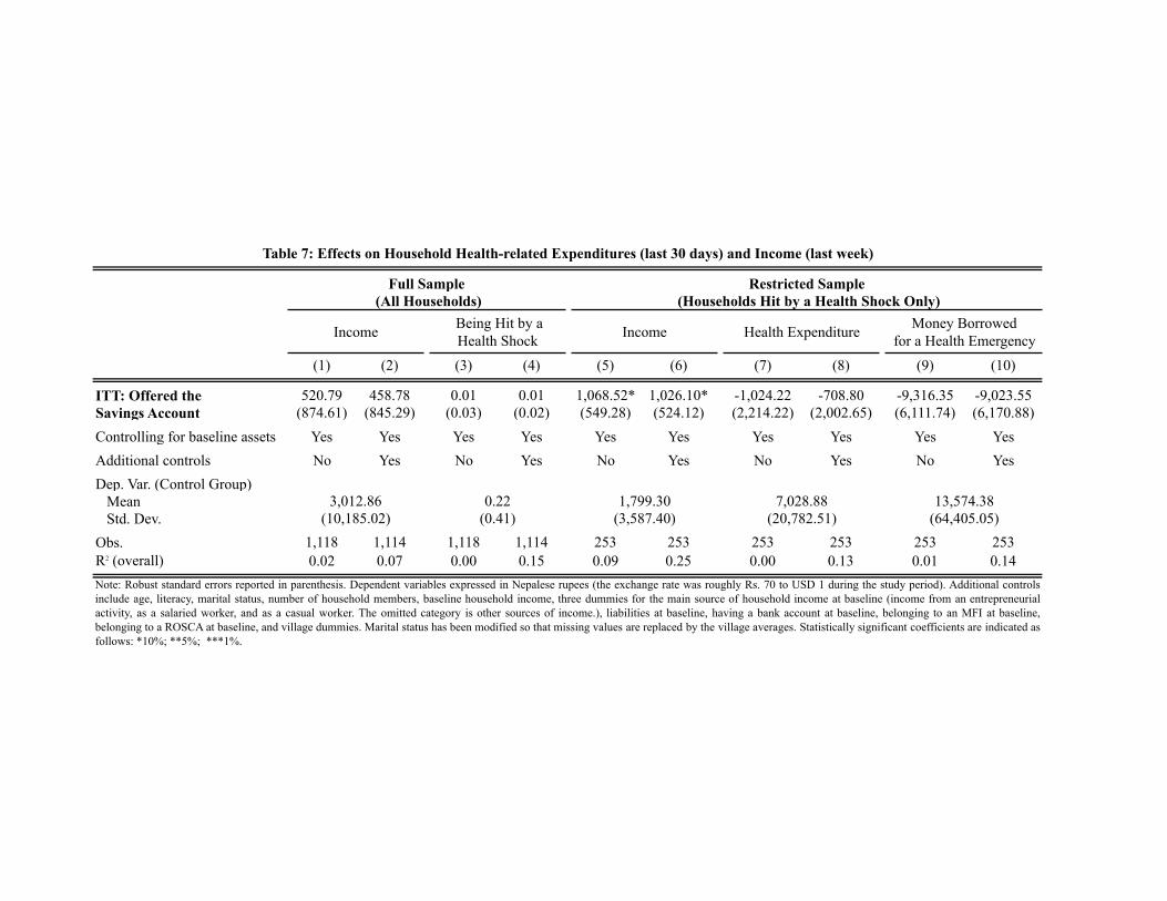
(1) (2) (3) (4) (5) (6) (7) (8) (9) (10)
ITT: Offered the 520.79 458.78 0.01 0.01 1,068.52* 1,026.10* -1,024.22 -708.80 -9,316.35 -9,023.55Savings Account (874.61) (845.29) (0.03) (0.02) (549.28) (524.12) (2,214.22) (2,002.65) (6,111.74) (6,170.88)Controlling for baseline assets Yes Yes Yes Yes Yes Yes Yes Yes Yes YesAdditional controls No Yes No Yes No Yes No Yes No YesDep. Var. (Control Group) Mean Std. Dev. Obs. 1,118 1,114 1,118 1,114 253 253 253 253 253 253R2 (overall) 0.02 0.07 0.00 0.15 0.09 0.25 0.00 0.13 0.01 0.14
Table 7: Effects on Household Health-related Expenditures (last 30 days) and Income (last week)
Note: Robust standard errors reported in parenthesis. Dependent variables expressed in Nepalese rupees (the exchange rate was roughly Rs. 70 to USD 1 during the study period). Additional controlsinclude age, literacy, marital status, number of household members, baseline household income, three dummies for the main source of household income at baseline (income from an entrepreneurialactivity, as a salaried worker, and as a casual worker. The omitted category is other sources of income.), liabilities at baseline, having a bank account at baseline, belonging to an MFI at baseline,belonging to a ROSCA at baseline, and village dummies. Marital status has been modified so that missing values are replaced by the village averages. Statistically significant coefficients are indicated asfollows: *10%; **5%; ***1%.
(10,185.02) (0.41)
Income
3,012.86 0.22(3,587.40)
Restricted Sample (Households Hit by a Health Shock Only)
Health Expenditure
7,028.88 13,574.38(20,782.51) (64,405.05)
Money Borrowed for a Health Emergency
Full Sample
Income Being Hit by a Health Shock
(All Households)
1,799.30
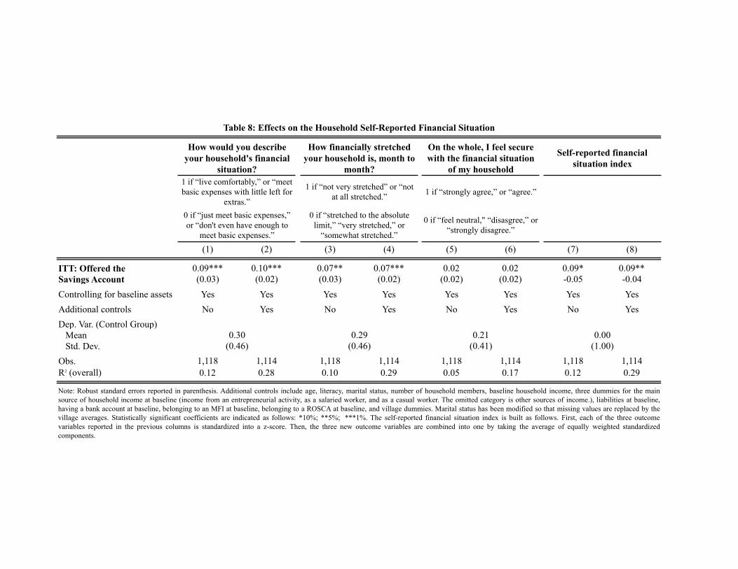
(1) (2) (3) (4) (5) (6) (7) (8)
ITT: Offered the 0.09*** 0.10*** 0.07** 0.07*** 0.02 0.02 0.09* 0.09**Savings Account (0.03) (0.02) (0.03) (0.02) (0.02) (0.02) -0.05 -0.04Controlling for baseline assets Yes Yes Yes Yes Yes Yes Yes YesAdditional controls No Yes No Yes No Yes No YesDep. Var. (Control Group) Mean Std. Dev. Obs. 1,118 1,114 1,118 1,114 1,118 1,114 1,118 1,114R2 (overall) 0.12 0.28 0.10 0.29 0.05 0.17 0.12 0.29
Note: Robust standard errors reported in parenthesis. Additional controls include age, literacy, marital status, number of household members, baseline household income, three dummies for the mainsource of household income at baseline (income from an entrepreneurial activity, as a salaried worker, and as a casual worker. The omitted category is other sources of income.), liabilities at baseline,having a bank account at baseline, belonging to an MFI at baseline, belonging to a ROSCA at baseline, and village dummies. Marital status has been modified so that missing values are replaced by thevillage averages. Statistically significant coefficients are indicated as follows: *10%; **5%; ***1%. The self-reported financial situation index is built as follows. First, each of the three outcomevariables reported in the previous columns is standardized into a z-score. Then, the three new outcome variables are combined into one by taking the average of equally weighted standardizedcomponents.
0.30(0.46)
0.29(0.46)
0.00(1.00)
0.21(0.41)
Table 8: Effects on the Household Self-Reported Financial Situation
How would you describe your household's financial
situation?
How financially stretched your household is, month to
month?
Self-reported financial situation index
1 if “live comfortably,” or “meet basic expenses with little left for
extras.”0 if “just meet basic expenses,” or “don't even have enough to
meet basic expenses.”
1 if “not very stretched” or “not at all stretched.”
0 if “stretched to the absolute limit,” “very stretched,” or
“somewhat stretched.”
On the whole, I feel secure with the financial situation
of my household
1 if “strongly agree,” or “agree.”
0 if “feel neutral," “disasgree,” or “strongly disagree.”

(1) (2)
ITT: Offered the Savings Account 0.014 0.013(0.017) (0.016)
Age of female household head 0.000(0.001)
Literacy -0.011(0.019)
Marital status1 0.009(0.031)
Number of household members 0.005(0.005)
Household income 0.000(0.000)
Income from an entrepreneurial activity 0.007(0.025)
Income as a salaried worker 0.026(0.027)
Income as a casual worker 0.001(0.021)
Constant 0.897*** 0.826***(0.012) (0.066)
Village dummies No YesObs. 1,236 1,224R2 (overall) 0.001 0.053Mean of dependent variable
Completed Endline
Appendix Table A1: Attrition
0.91
Note: Robust standard errors, reported in parenthesis. 1Marital status has been modified so that missingvalues are replaced by the village averages. The omitted category for the main source of householdincome is other sources of income. Statistically significant coefficients are indicated as follows: *10%;**5%; ***1%.
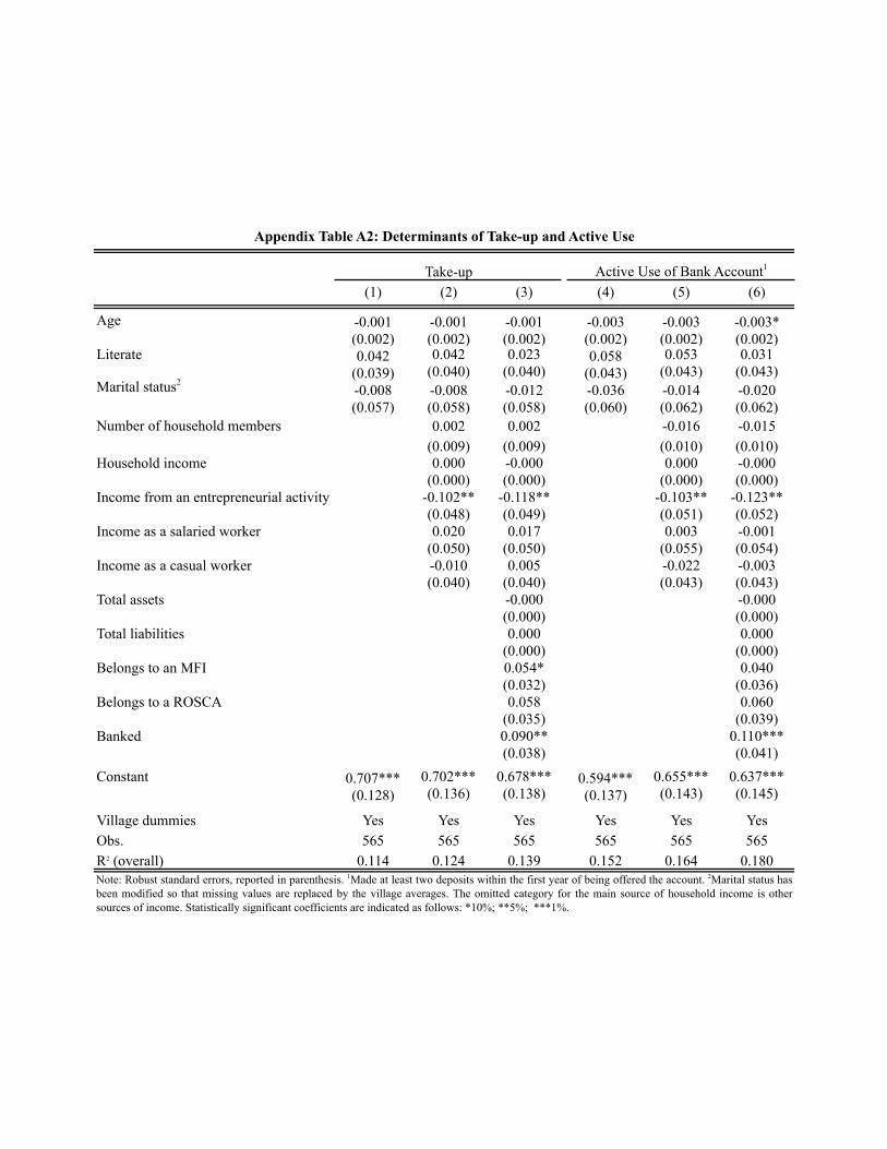
(1) (2) (3) (4) (5) (6)
Age -0.001 -0.001 -0.001 -0.003 -0.003 -0.003*(0.002) (0.002) (0.002) (0.002) (0.002) (0.002)
Literate 0.042 0.042 0.023 0.058 0.053 0.031(0.039) (0.040) (0.040) (0.043) (0.043) (0.043)-0.008 -0.008 -0.012 -0.036 -0.014 -0.020(0.057) (0.058) (0.058) (0.060) (0.062) (0.062)
Number of household members 0.002 0.002 -0.016 -0.015(0.009) (0.009) (0.010) (0.010)
Household income 0.000 -0.000 0.000 -0.000(0.000) (0.000) (0.000) (0.000)
Income from an entrepreneurial activity -0.102** -0.118** -0.103** -0.123**(0.048) (0.049) (0.051) (0.052)
Income as a salaried worker 0.020 0.017 0.003 -0.001(0.050) (0.050) (0.055) (0.054)
Income as a casual worker -0.010 0.005 -0.022 -0.003(0.040) (0.040) (0.043) (0.043)
Total assets -0.000 -0.000(0.000) (0.000)
Total liabilities 0.000 0.000(0.000) (0.000)
Belongs to an MFI 0.054* 0.040(0.032) (0.036)
Belongs to a ROSCA 0.058 0.060(0.035) (0.039)
Banked 0.090** 0.110***(0.038) (0.041)
Constant 0.707*** 0.702*** 0.678*** 0.594*** 0.655*** 0.637***(0.128) (0.136) (0.138) (0.137) (0.143) (0.145)
Village dummies Yes Yes Yes Yes Yes YesObs. 565 565 565 565 565 565R2 (overall) 0.114 0.124 0.139 0.152 0.164 0.180Note: Robust standard errors, reported in parenthesis. 1Made at least two deposits within the first year of being offered the account. 2Marital status hasbeen modified so that missing values are replaced by the village averages. The omitted category for the main source of household income is othersources of income. Statistically significant coefficients are indicated as follows: *10%; **5%; ***1%.
Marital status2
Appendix Table A2: Determinants of Take-up and Active Use
Take-up Active Use of Bank Account1

Savings Motives % of account holders
To pay for a health emergency 88.25To buy food when income is low 65.85To pay for school fees or school material 49.89To pay for a festival 18.40To repay a debt 9.98To pay for home maintenance 7.10To invest in my current business 6.21To buy poultry or livestock 6.21To buy agricultural inputs (pesticides, fertilizer, etc.) 5.10To pay bills 4.88To start a new business 3.33Other 2.88To pay for a funeral 2.00To buy gold 1.33
Savings Account Characteristics % of account holders
Easy to deposit and withdraw any amount of money any time 70.18The account is simple to understand 13.23Trust 8.97Bank opens twice a week in the community 3.59Bank has a female employee 2.69Cannot open a savings account in another bank/fin. institution 0.67The account offers a high interest rate 0.45Don't know any other financial institution 0.22Do not feel confident opening a savings account in another bank/fin. institution 0.00Do not know how to open a savings account in another bank/fin. institution 0.00Total 100.00
Appendix Table A3: Savings Account Characteristics and Savings Motives
Panel B: Most Valued Feature of the Savings Account
Panel A: Reasons for Saving in the Account (Multiple Choice)1
1Percentages for the savings motives do not add up to 100 as households could select more than one savings motive.
Recommended