PNNL-17424

S-102 Transfer Pump Restriction Modeling Results B. E. Wells K. I. Johnson D. R. Rector D. S. Trent March 2008 Prepared for the U.S. Department of Energy under Contract DE-AC05-76RL01830

DISCLAIMER This report was prepared as an account of work sponsored by an agency of the United States Government. Neither the United States Government nor any agency thereof, nor Battelle Memorial Institute, nor any of their employees, makes any warranty, express or implied, or assumes any legal liability or responsibility for the accuracy, completeness, or usefulness of any information, apparatus, product, or process disclosed, or represents that its use would not infringe privately owned rights. Reference herein to any specific commercial product, process, or service by trade name, trademark, manufacturer, or otherwise does not necessarily constitute or imply its endorsement, recommendation, or favoring by the United States Government or any agency thereof, or Battelle Memorial Institute. The views and opinions of authors expressed herein do not necessarily state or reflect those of the United States Government or any agency thereof. PACIFIC NORTHWEST NATIONAL LABORATORY operated by BATTELLE for the UNITED STATES DEPARTMENT OF ENERGY under Contract DE-ACO5-76RL01830

Printed in the United States of America

Available to DOE and DOE contractors from the Office of Scientific and Technical Information,

P.O. Box 62, Oak Ridge, TN 37831-0062; ph: (865) 576-8401 fax: (865) 576 5728

email: reports@adonis.osti.gov

Available to the public from the National Technical Information Service, U.S. Department of Commerce, 5285 Port Royal Rd., Springfield, VA 22161

ph: (800) 553-6847 fax: (703) 605-6900

email: orders@nits.fedworld.gov online ordering: http://www.ntis.gov/ordering.htm

PNNL-17424

S-102 Transfer Pump Restriction Modeling Results B. E. Wells K. I. Johnson D. R. Rector D. S. Trent March 2008 Prepared for the U.S. Department of Energy under Contract DE-AC05-76RL01830 Pacific Northwest National Laboratory Richland, Washington

iii

Summary

CH2M HILL Hanford Group has postulated that a radioactive waste leak in the Hanford S-Farm in the vicinity of the S-102 retrieval pump discharge occurred because of over-pressurization and failure of the S-102 dilution water-supply hose while operating the retrieval pump in reverse with an obstructed suction cavity and an unobstructed flow path to the dilution water-supply hose. CH2M HILL asked Pacific Northwest National Laboratory (PNNL) to identify and evaluate plausible scenarios and physical mechanisms for the obstruction and resulting waste leak. This report describes computational modeling results for the pressure in the retrieval pump suction cavity at the dilution line inlet. The results suggest that there are plausible scenarios and conditions that could result in a pressure at the dilution line inlet approaching 400 psi. The retrieval pump operations before the leak event are summarized in Section 2 to establish the scenario conditions. The computational modeling methods are described, and results are presented in Section 3. A summary of the model results is provided in Section 4. Appendix A describes two validation cases that were completed with the PNNL lattice kinetics computer program that were used to model the pump sediment formation. Appendix B describes test problems that were distributed with the Marc finite element software to confirm that the correct solution of material models and contact conditions were used to simulate the initial yielding and flow of waste plugging the inlet of the positive displacement pump in Tank S-102. Appendix C presents certain TEMPEST calculations of fluid dynamic pressure compared to known analytical and empirical results to establish the extent of the code’s accuracy in such cases.

v

Acronyms and Abbreviations

CFD computational fluid dynamic (code)

cm centimeter

ft foot

g gram

gpm gallons per minute

in. inch

lb pound

µ micron

mL milliliter

µm micrometer

MPa mega pascal

Pa Pascal

Pa-s Pascal seconds

PNNL Pacific Northwest National Laboratory

psi pounds per square inch

sec or s second

SSC structure, system, or component

VFD variable frequency drive

vol% volume percent

vii

Contents

Summary ...................................................................................................................................................... iii

Acronyms and Abbreviations ....................................................................................................................... v

1.0 Introduction........................................................................................................................................ 1.1

2.0 Model Inputs and Approach............................................................................................................... 2.1

2.1 Event Summary .......................................................................................................................... 2.1

2.2 Pump Geometry.......................................................................................................................... 2.2

2.3 Waste Properties......................................................................................................................... 2.4

2.4 Modeling Cases .......................................................................................................................... 2.6

3.0 Model Results .................................................................................................................................... 3.1

3.1 Restriction Formation................................................................................................................. 3.1 3.1.1 Code Description ............................................................................................................. 3.1 3.1.2 Validation Test Cases ...................................................................................................... 3.3 3.1.3 Simulation Results ........................................................................................................... 3.3 3.1.4 Restriction Formation Modeling Discussion ................................................................. 3.11

3.2 Restriction Failure .................................................................................................................... 3.14 3.2.1 Test Cases ...................................................................................................................... 3.14 3.2.2 The Material Properties Estimated for Sedimentary Waste........................................... 3.15 3.2.3 Case 1, Failure of Waste in the Pump Column Only ..................................................... 3.16 3.2.4 Case 2, Failure of Waste in the Pump Column with a Waste-Filled Annulus

Around the Pump ........................................................................................................... 3.20 3.2.5 Case 3, Failure of Waste in the Pump Column with a Continuous Waste Mass

Around the Pump ........................................................................................................... 3.24 3.2.6 Additional Cases with Reduced Waste Height and Applied Pressure Loading............. 3.27 3.2.7 Restriction Failure Discussion ....................................................................................... 3.31

3.3 Restriction Flow ....................................................................................................................... 3.31 3.3.1 Test Cases ...................................................................................................................... 3.31 3.3.2 TEMPEST Simulation Models ...................................................................................... 3.31 3.3.3 Simulation Parameters ................................................................................................... 3.35 3.3.4 Pressure Calculations..................................................................................................... 3.36 3.3.5 Restriction Flow Discussion .......................................................................................... 3.37

4.0 Summary ............................................................................................................................................ 4.1

5.0 References .......................................................................................................................................... 5.1

Appendix A: Test Cases for Sediment Formation .................................................................................... A.1

viii

Appendix B: Validation of the Marc Finite Element Code for Simulating Sediment Yielding in the Static Pump Test ..........................................................................................................................B.1

Appendix C. TEMPEST Testing for Pressure Calculation.......................................................................C.1

Figures

2.1. Depiction of S-102 Waste Transfer System (CH2M HILL 2007).................................................... 2.2

2.2. As-Modeled S-102 Pump Geometry................................................................................................. 2.3

3.1. Flow and Pressure (Pa) Distributions at Beginning of Cycle 1 ........................................................ 3.5

3.2. Flow and Pressure (Pa) Distributions at End of Cycle 1................................................................... 3.5

3.3. Pressure as a Function of Time for Case 1, Cycle 2 ......................................................................... 3.7

3.4. Sediment Bed (initial velocities zero) at t = 0 Seconds for Case 1, Cycle 2..................................... 3.7

3.5. Sediment Bed and Velocities at t = 50 Seconds for Case 1, Cycle 2................................................ 3.8

3.6. Sediment Bed and Velocities at t = 0 sec. for Case 2 ..................................................................... 3.10

3.7. Pressure as a Function of Time for Cases 2 and 3 .......................................................................... 3.11

3.8. Sediment Bed and Velocities at t = 4 Seconds for Case 3 .............................................................. 3.12

3.9. Sediment Bed and Velocities at t = 4 sec. for Case 3 ..................................................................... 3.13

3.10. Contour Plot of the Shear Stress Distribution in the Waste as it Extrudes from the Pump Inlet Slot: Case 1.1.......................................................................................................................... 3.19

3.11. The Case 1 Finite Element Model of the Waste Filling the Bottom Section of the S-102 Pump Column ................................................................................................................................. 3.17

3.12. Contour Plot of the Pressure Distribution (mean normal stress) in the Waste as it Extrudes from the Pump Inlet Slot: Case 1.1................................................................................................. 3.19

3.13. Pressure Versus Compressive Displacement of the Waste Column ............................................... 3.20

3.14. The Case 2 Model of Waste in the Pump Column with Waste Filling an Annulus Around the Pump ......................................................................................................................................... 3.21

3.15. Pressure Versus Waste-Column Displacement Plots Comparing Cases 2.1 and 2.2 (with waste in the outside annulus) and Case 1.1 and 1.2 (no waste in the outside annulus) .................. 3.22

3.16. The Final Deformed Shape of Sensitivity Case 2.1 Showing the Distribution of Pressure (mean normal stress) in the Waste as it Extrudes from the Pump Inlet Slot into the Annulus Around the Pump............................................................................................................................ 3.23

ix

3.17. The Shear Stress Distribution for Case 2.1 Showing the Waste Being Extruded from the Pump Slot Upward into the Annulus Around the Pump................................................................. 3.23

3.18. The Case 3 Model of Waste in the Pump Column with a Large Waste Mass Surrounding the Pump ......................................................................................................................................... 3.25

3.19. Pressure Versus Waste Column Displacement Plots Comparing Cases 3.1 and 3.2 (a large diameter mass of waste outside the pump) with Cases 2.1 and 2.2 (2-inch waste filled annulus) and Case 1.7 and 1.8 (no waste outside the pump) .......................................................... 3.25

3.20. The Final Pressure Distribution (mean normal stress) in Case 3.1 as the Waste Extrudes from the Pump Inlet Slot Upward into the Large Waste Mass Around the Pump.......................... 3.26

3.21. The Final Shear Stress Distribution in Case 3.1 ............................................................................. 3.26

3.22. Model with Short Waste Column and Pressure Loading................................................................ 3.28

3.23. Deformed Shape of the Waste Column at a Pressure of 1.4 MPa (203 psi) ................................... 3.29

3.24. Model with Short Waste Column and Pressure Loading................................................................ 3.30

3.25. Deformed Shape of the Waste Column at a Pressure of 1.6 MPa (232 psi) ................................... 3.30

3.26. System Geometry Modeled in TEMPEST for all Cases Simulated................................................ 3.32

3.27. TEMPEST Noding Grid Overlaid on Assumed Waste Distribution for Case 1—Settled Waste in Pump, Water in Annulus.................................................................................................. 3.33

3.28. TEMPEST Noding Grid Overlaid on Assumed Waste Distribution for Case 2—Settled Waste in Pump and Annulus........................................................................................................... 3.34

3.29. TEMPEST Noding Grid Overlaid on Assumed Waste Distribution for Case 3—Settled Waste in Pump, External Waste Domain Extending to Edge of Tank ........................................... 3.35

x

Tables

2.1. Solid Phase Compounds in S-102 Sludge......................................................................................... 2.4

2.2. Summary of Waste Properties .......................................................................................................... 2.6

3.1. Elastic Modulus of Selected Soil Types ......................................................................................... 3.15

3.2. Poisson’s Ratio of Selected Soil Types .......................................................................................... 3.15

3.3. Internal Friction Angle for a Selection of Soil Types..................................................................... 3.16

3.4. Input Data for Cases 1.1 Though 1.4 of the Waste Yielding Model............................................... 3.18

3.5. Input Data for Cases 2.1 and 2.2 of the Waste Yielding Model ..................................................... 3.20

3.6. Input Data for Cases 3.1 and 3.2 of the Waste Yielding Model ..................................................... 3.24

3.7. Pump Pressure Time History: 20 gpm............................................................................................ 3.36

3.8. Pump Pressure Time History: 30 gpm............................................................................................ 3.36

4.1. Pressure Results at Dilution Line Inlet ............................................................................................. 4.2

1.1

1.0 Introduction

On July 27, 2007, a radioactive waste leak was reported to have occurred in the Hanford S-Farm in the vicinity of the S-102 retrieval pump discharge (CH2M HILL 2007). CH2M HILL Hanford Group has postulated that the leak occurred because of over-pressurization and failure of the S-102 dilution water-supply hose while operating the retrieval pump in reverse with an obstructed suction cavity and an unobstructed flow path to the dilution water-supply hose. Pressure in the retrieval-pump-suction cavity at the dilution line inlet due to obstruction or restriction was investigated to identify plausible scenarios via computational modeling that could result in a pressure sufficient to fail the dilution water-supply hose. The specific pressure at which the dilution line failed is unknown. However, the dilution system is not designed to withstand the retrieval-pump discharge pressure (CH2M HILL 2007). In addition to the limit of the available pressure (i.e. the capability of the retrieval-pump), the pump column should uplift, thereby releasing pressure in the suction cavity, when the pressure required to lift the pump is reached.(a) This phenomena is not considered in this analysis. In Section 2, the retrieval-pump operations before the leak event are summarized to establish the scenario conditions. The retrieval pump and waste conditions as understood are documented on a "best-estimate" basis. Three modeling cases representing plausible initial conditions for the over-pressurization event are evaluated. In Section 3, the computational modeling methods are described, and results are presented. The restriction formation was modeled using the lattice Boltzmann method, restriction failure was modeled using the Marc finite element code, and the restriction flow was modeled using the TEMPEST finite-volume computational fluid dynamic (CFD) code. The software used for the analyses is identified as “non-safety software” in that results provided from the software models are not to be used in any nuclear-safety related manner for design, monitoring, and/or administrative functions of a nuclear facility. The results will not ensure the proper accident or hazards analysis of a nuclear facility or a structure, system, or component (SSC) that performs a safety function. A summary of the model results is provided in Section 4. As stated above, the purpose of this work is to identify plausible scenarios; all results must be treated as qualitative.

(a) E-mail correspondence from WB Barton to BE Wells, 3/20/08, 3:19 PM.

2.1

2.0 Model Inputs and Approach

Retrieval-pump operations before the leak event are summarized to establish the scenario conditions in Section 2.1. The retrieval-pump configuration as modeled is presented in Section 2.2. Modeled waste conditions are documented in Section 2.3, and the modeling cases are presented in Section 2.4.

2.1 Event Summary

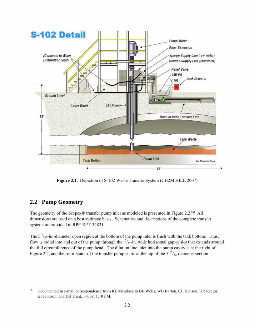
Waste is retrieved from S-102 to SY-102 using a positive displacement progressive cavity Seepex® pump. For reference, a depiction of the waste transfer system at S-102 is provided in Figure 2.1. Waste is mobilized to the transfer pump via water nozzles. At the time of the leak event, approximately 8% of the original waste volume remained in the tank in the form of an 18-inch-deep “waste heel” (CH2M HILL 2007). As presented in the CH2M HILL (2007) report, normal retrieval operations proceeded from approximately 16:00 to 18:20 on July 26, 2007. At nominally 18:20, the transfer pump automatically shut down because of a ground-fault indication on the pump’s variable frequency drive (VFD) panel. Waste mobilization to the transfer pump via the water nozzles continued for approximately 8 minutes after the electrical shut-down. The electrical shut-down precluded the normal “Stop with Auto Reverse,” which returns the pump column and transfer line slurry back into S-102. Thus, approximately 230 gal of slurry remained in the pump column and transfer line. At approximately 21:45, the transfer line to SY-102 was flushed with water, leaving nominally 110 gallons of slurry in the pump column and 110 gallons of water in the transfer line. After 22:00, the ground-fault indication on the VFD was cleared. The pump would not operate and was determined to be “bound.” A maintenance crew entered S-Farm and began the process of manually turning the pump shaft in the reverse direction at nominally 23:30. After several unsuccessful attempts to run the pump in reverse, alternating with manual rotations, the pump ran in reverse for 105 seconds(a) at approximately 01:25 and again at 02:00 on July 27, 2007. Since the pump appeared to be running correctly, the maintenance crew exited S-Farm at approximately 02:05. A third reverse-pump operation of 105 seconds was conducted at approximately 02:10. High motor current, as compared to normal transfer-pump operations, occurred during all three reverse-pump operations until approximately 20 seconds into the third reverse-pump operation, at which point, the current returned to normal operating conditions.(b) The leak event is understood to have occurred during this third reverse-pump operation.

(a) The programmed time for a reverse run of the pump is 105 sec to clear approximately 230 gal of slurry out of the

pump column and transfer line. (b) WB Barton, Technical Review of S-102 Spill Scenario meeting, August 9, 2007.

2.2

Figure 2.1. Depiction of S-102 Waste Transfer System (CH2M HILL 2007)

2.2 Pump Geometry

The geometry of the Seepex® transfer pump inlet as modeled is presented in Figure 2.2.(a) All dimensions are used on a best-estimate basis. Schematics and descriptions of the complete transfer system are provided in RPP-RPT-34831. The 5 9/32-in.-diameter open region at the bottom of the pump inlet is flush with the tank bottom. Thus, flow is radial into and out of the pump through the 17/32-in. wide horizontal gap or slot that extends around the full circumference of the pump head. The dilution line inlet into the pump cavity is at the right of Figure 2.2, and the rotor-stator of the transfer pump starts at the top of the 5 29/32-diameter section.

(a) Documented in e-mail correspondence from RE Mendoza to BE Wells, WB Barton, CE Hanson, DR Rector,

KI Johnson, and DS Trent, 1/7/08, 1:10 PM.

2.3

Figure 2.2. As-Modeled S-102 Pump Geometry

2.4

2.3 Waste Properties

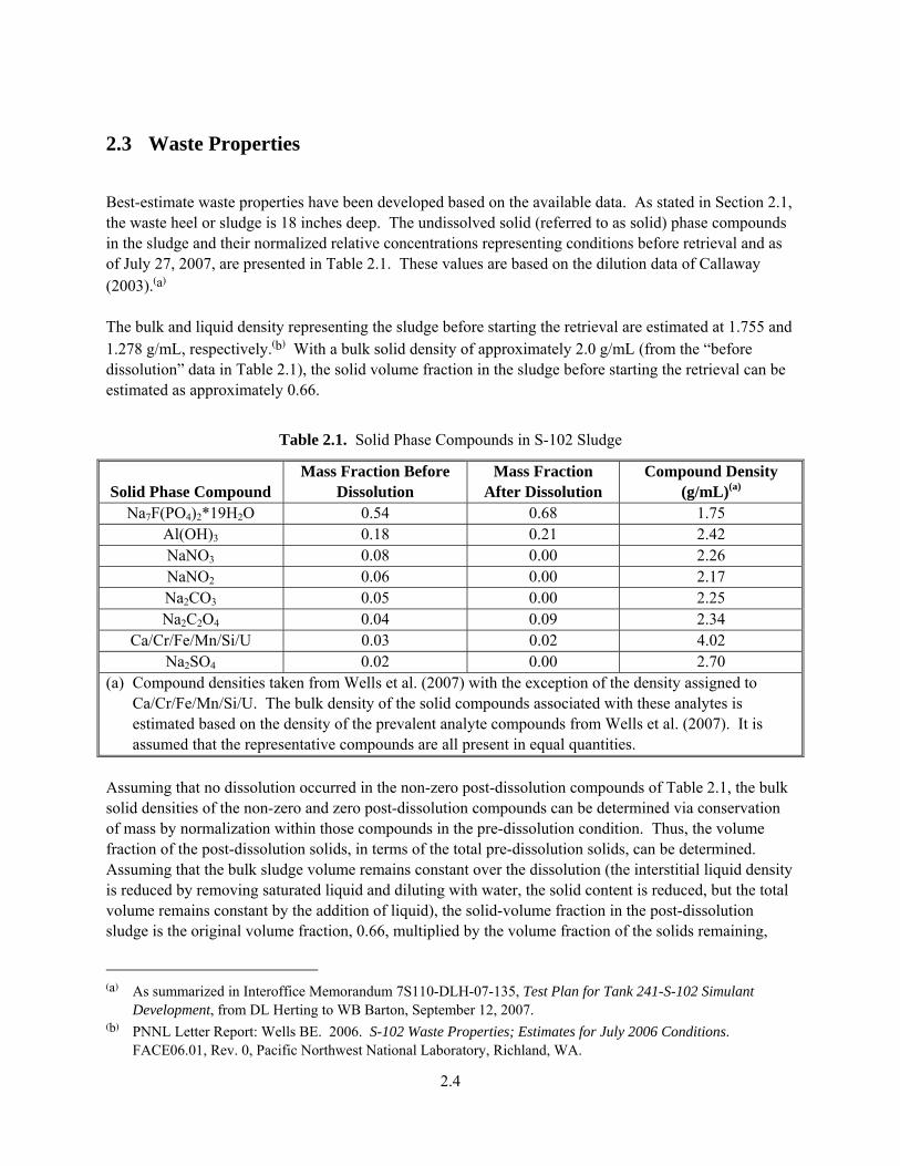
Best-estimate waste properties have been developed based on the available data. As stated in Section 2.1, the waste heel or sludge is 18 inches deep. The undissolved solid (referred to as solid) phase compounds in the sludge and their normalized relative concentrations representing conditions before retrieval and as of July 27, 2007, are presented in Table 2.1. These values are based on the dilution data of Callaway (2003).(a) The bulk and liquid density representing the sludge before starting the retrieval are estimated at 1.755 and 1.278 g/mL, respectively.(b) With a bulk solid density of approximately 2.0 g/mL (from the “before dissolution” data in Table 2.1), the solid volume fraction in the sludge before starting the retrieval can be estimated as approximately 0.66.

Table 2.1. Solid Phase Compounds in S-102 Sludge

Solid Phase Compound Mass Fraction Before

Dissolution Mass Fraction

After Dissolution Compound Density

(g/mL)(a) Na7F(PO4)2*19H2O 0.54 0.68 1.75

Al(OH)3 0.18 0.21 2.42 NaNO3 0.08 0.00 2.26 NaNO2 0.06 0.00 2.17 Na2CO3 0.05 0.00 2.25 Na2C2O4 0.04 0.09 2.34

Ca/Cr/Fe/Mn/Si/U 0.03 0.02 4.02 Na2SO4 0.02 0.00 2.70

(a) Compound densities taken from Wells et al. (2007) with the exception of the density assigned to Ca/Cr/Fe/Mn/Si/U. The bulk density of the solid compounds associated with these analytes is estimated based on the density of the prevalent analyte compounds from Wells et al. (2007). It is assumed that the representative compounds are all present in equal quantities.

Assuming that no dissolution occurred in the non-zero post-dissolution compounds of Table 2.1, the bulk solid densities of the non-zero and zero post-dissolution compounds can be determined via conservation of mass by normalization within those compounds in the pre-dissolution condition. Thus, the volume fraction of the post-dissolution solids, in terms of the total pre-dissolution solids, can be determined. Assuming that the bulk sludge volume remains constant over the dissolution (the interstitial liquid density is reduced by removing saturated liquid and diluting with water, the solid content is reduced, but the total volume remains constant by the addition of liquid), the solid-volume fraction in the post-dissolution sludge is the original volume fraction, 0.66, multiplied by the volume fraction of the solids remaining,

(a) As summarized in Interoffice Memorandum 7S110-DLH-07-135, Test Plan for Tank 241-S-102 Simulant

Development, from DL Herting to WB Barton, September 12, 2007. (b) PNNL Letter Report: Wells BE. 2006. S-102 Waste Properties; Estimates for July 2006 Conditions.

FACE06.01, Rev. 0, Pacific Northwest National Laboratory, Richland, WA.

2.5

0.81, resulting in a volume fraction of approximately 0.54. With an interstitial liquid density of 1.03 g/mL, the estimated bulk density of the July 27, 2007, sludge is therefore 1.51 g/mL.(a) The density of the solid phase is approximately 1.93 g/mL. The particle-size distribution of the sludge solids is estimated from scanning electron microscopy (SEM) results.(b,c) Approximately 68 wt% of the solids are Na7F(PO4)2*19H2O (0.1 to 200 μm, 100-μm average) at 1.75 g/mL, approximately 21 wt% Al(OH)3 (20 to 200 μm) at 2.42 g/mL, approximately 9 wt% Na2C2O4 (< 20 μm) at 2.34 g/mL (order of 1 wt% that will go into solution with 20 wt% free water in bulk is ignored; see data source), and approximately 2 wt% (<20 μm) at approximately 4.02 g/mL. Assuming that the Na7F(PO4)2*19H2O is uniformly distributed over its particle-size range, it can be determined that the volume distribution of the solids is approximately 16% < 20 μm at 2.2 g/mL and 84% 20 to 200 μm at 1.9 g/mL. The inherent limitations of using SEM to develop a particle size distribution are acknowledged.(d) This approach is used in lieu of any other data source. The particle size distribution affects the sediment formation simulations described in Section 3.1 in two different ways. First, the hindered settling rate controls the rate of growth of sediment inside the pump and the annulus. The base settling rate goes as the square of the particle diameter. Therefore, a doubling of the particle diameter will result in a quadrupling of the settling velocity. As a result, the sediment profile will increase in elevation more quickly and reach a higher equilibrium elevation. Secondly, the flow resistance through the sediment bed, as calculated by the Ergun equation, is a function of the average particle diameter. The dominant term in the Ergun expression (for the range of velocities we are interested in) is proportional to the inverse diameter squared. As the diameter decreases by a factor of two, the flow resistance increases and the pressure drop for the same flow rate is higher by approximately a factor of four. The slurry in the pump column when the transfer pump initially shut down before the leak event (see Section 2.1) had a bulk density of 1.08 g/mL with a liquid density of 1.03 g/mL.(e) With a solid density of 1.93 g/mL (see above), the solid volume fraction in the slurry is thus 0.06. No liquid or slurry viscosity data specific to the waste in S-102 are available. Thus, the slurry viscosity model recommended by Jewett et al. (2002) for use in analyzing the waste-feed delivery transfer system is used to provide a reasonable representation(f) of the quantity for this analysis. The form of the correlation is:

(a) E-mail correspondence from WB Barton to BE Wells, 1/18/08, 1:56 PM. (b) Documented in e-mail correspondence from WB Barton to BE Wells, DL Herting, RE Mendoza, CE Hanson,

DR Rector, DS Trent, KI Johnson, and JE Meacham, 1/16/08, 7:30 AM. (c) As reported in Interoffice Memorandum 7S110-DLH-07-135, Test Plan for Tank 241-S-102 Simulant

Development, from DL Herting to WB Barton, September 12, 2007. (d) Limitations include: representativeness of sample, representativeness of particulate evaluated, spatial resolution

of instrumentation used in analyses, beam voltage (which impacts the visibility of surface features), and orientation of the particles relative to the probe.

(e) Slurry density of 1.08 g/mL reported in “S-102 Time Line Observations” provided at Technical Review of S-102 Spill Scenario meeting, August 9, 2007.

(f) Viscosity model documented in e-mail correspondence from BE Wells to WB Barton to DL Herting, RE Mendoza, CE Hanson, DR Rector, DS Trent, KI Johnson, and JE Meacham, 1/23/08, 6:34 PM.

2.6

( )( )[ ] 1v17Cexp1.3v10.5Cv2.5C1002.0 06.02 −γ−+++=μ (2.1)

where the viscosity is in units of Pa-s, Cv is the solid volume fraction, and γ is the strain rate (s-1). The liquid viscosity is determined via Eq. (2.1) with zero solid content. The shear strength of the sludge at 0.54 volume fraction, 1,200 Pa, is the median result from core extrusion estimates for pre-retrieval conditions.(a,b) The best-estimate waste properties used in modeling the leak event are summarized in Table 2.2.

Table 2.2. Summary of Waste Properties

Waste Property Value or Reference (units) Liquid Density 1.03 (g/mL)

Bulk Density, Sludge 1.51 (g/mL) Bulk Density, Slurry 1.08 (g/mL)

Solid Density 1.93 (g/mL) Solid Volume Fraction, Sludge 0.54 Solid Volume Fraction, Slurry 0.06

Solid Particle-Size Distribution (by volume fraction)

0.16 at < 20 μm, 2.2 (g/mL) 0.84 20 to 200 μm, (1.9 g/mL)

Liquid Viscosity Equation 2.1 with Cv = 0 Slurry Viscosity Equation 2.1 Shear Strength 1,200 (Pa)

2.4 Modeling Cases

When the reverse-pump operation started, as described in the event summary of Section 2.1, the transfer pump and line contained nominally 110 gallons of slurry and 110 gallons of water, respectively. Outside of the pump, the sludge was 18 inches deep, and the sludge was separated from the pump column by an annular region approximately 2 inches wide.(c) Three cases are considered:

• Case 1. Fixed boundary, water in annulus, slurry in pump column. • Case 2. Fixed boundary, sludge in annulus, slurry in pump column. • Case 3. Sludge boundary and in annulus, slurry in pump column.

(a) PNNL Letter Report: Wells BE. 2006. S-102 Waste Properties; Estimates for July 2006 Conditions.

FACE06.01, Rev. 0, Pacific Northwest National Laboratory, Richland, WA. (b) Shear strength documented in e-mail correspondence from BE Wells to WB Barton to DL Herting,

RE Mendoza, CE Hanson, DR Rector, DS Trent, KI Johnson, and JE Meacham, 1/17/08, 10:59 AM. (c) WB Barton, Technical Review of S-102 Spill Scenario meeting, August 9, 2007.

2.7

“Fixed Boundary” refers to the wall of sludge 18 inches deep that begins 2 inches outside of the pump column. The 2-inch region is assumed to have a vertical outer wall and extends from the outside diameter of the pump column, which is 9 29/32 inches (Figure 2.2). When treated as a fixed boundary, the sludge forming the outer wall of the annulus cannot be mobilized by flow in the annulus. Case 1 represents the least restrictive condition possible in that resistance to reverse flow from the pump will only be developed by the slurry in the pump column. However, given that transfer operations were proceeding at the time of the pump shut-down, and that waste continued to be mobilized to the transfer pump for a short period of time after the shut-down (see Section 2.1), it is reasonable to expect that the annular region contained waste material, and thus, the conditions for Case 2 exist. As the exact quantity of the waste in the annulus is unknown, the annulus is assumed to be “full,” and the material is represented as sludge. Case 3 differs from Case 2 in that there is no fixed boundary, and the annular constraint on reverse flow from the pump is removed.

3.1

3.0 Model Results

Three software models are employed to evaluate the restriction formation, bed failure, and subsequent flow, respectively, for each case (see Section 2.4). For each case, the pressure at the dilution line inlet is evaluated as the restriction is formed, fails, and flows in the pump inlet cavity, slot, and annulus. The results of the restriction formation model define the initial conditions for the model of restriction failure, which in turn provides initial conditions for the flow calculation. The models are exclusive in that the formation model does not predict when the sediment bed will fail and the failure model does not predict results from a flow condition. Thus, the model can be summarized as

• Restriction Formation: Pressure at dilution line inlet during sediment bed formation. Location of sediment bed for Failure and Flow.

• Restriction Failure: Pressure to yield sediment bed as a function of waste parameters. • Restriction Flow: Pressure at dilution line inlet during sediment bed flow after failure.

Modeling of the restriction formation using the lattice Boltzmann method is presented in Section 3.1. Restriction failure using the Marc finite element code is presented in Section 3.2. Restriction flow using the TEMPEST finite-volume CFD code is presented in Section 3.3.

3.1 Restriction Formation

The code used for the sediment formation simulations is described in Section 3.1.1. Validation test case results are presented in Section 3.1.2, and simulation results and discussion are provided in Sections 3.1.3 and 3.1.4 respectively.

3.1.1 Code Description

The sediment formation simulations were performed using a computer program developed at Pacific Northwest National Laboratory (PNNL) based on lattice kinetics, a variation of the lattice Boltzmann method. The lattice Boltzmann equation (Sukop and Thorne 2006 describes the evolution of the discretized particle-distribution function, fi(x,t), along direction i as a function of time, where x is location and t is time. The new time-distribution function is given by the equation

[ ])t,x(f)t,x(f1)t,x(f)tt,tex(f eq

iiiii −τ

−=−Δ+Δ+ (3.1)

where τ is a linear relaxation parameter, and feq is the local equilibrium distribution. The local equilibrium is expressed in the form of a quadratic expansion of the Maxwellian distribution

f ieq = wiρ 1+

3ei ⋅ uc 2 +

9(ei ⋅ u)2

2c 4 −3u2

2c 2

⎡

⎣ ⎢

⎤

⎦ ⎥ (3.2)

3.2

where c is the reference lattice speed and c=Δx/Δt and wi are the weight coefficients for each vector direction, u is the local velocity and ρ is the density. The lattice kinetics method differs from the lattice Boltzmann method in that the relaxation parameter, τ, is set equal to one, and additional terms are added to account for the difference in the viscous shear stress and Darcy flow-resistance terms.

The Darcy flow resistance associated with the sediment bed is determined using the Ergun equation

ΔpL

=150μ(1−ε)2 u0

ε3dp2 +

1.75(1−ε)ρu02

ε3dp

(3.3)

where ε is the bed porosity, u0 is the fluid superficial velocity, and dp is the average particle diameter. The average diameter for particle mixtures is calculated using the expression

dp =xi

dp,i∑

⎛

⎝ ⎜ ⎜

⎞

⎠ ⎟ ⎟

−1

(3.4)

where xii is the volume fraction of type i particles out of the total solid volume. The effect of turbulence is included using the k-ε model (Wilcox 1993), where the turbulent kinetic energy, k, and the dissipation rate, ε, are calculated by solving the coupled transport equations

∂k∂t

+ U j∂k∂x j

= τ ij∂Ui

∂x j

−ε +∂

∂x j

ν +νT

σ k

⎛

⎝ ⎜

⎞

⎠ ⎟

∂k∂x j

⎡

⎣ ⎢

⎤

⎦ ⎥ (3.5)

∂ε∂t

+ U j∂ε∂x j

= Cε1εk

τ ij∂Ui

∂x j

− Cε 2ε2

k+

∂∂x j

ν +νT

σε

⎛

⎝ ⎜

⎞

⎠ ⎟

∂ε∂x j

⎡

⎣ ⎢

⎤

⎦ ⎥ (3.6)

where νΤ is the kinematic eddy viscosity. νT = Cμk 2 /ε (3.7)

Separate continuum fields are used to represent the suspended solids for each particle size and the sediment bed. Each particle size is treated as a passive scalar with an associated transport equation. The rate of hindered settling is given by the expression

u =2d2(ρs − ρl )g

9μ1−

φφref

⎛

⎝ ⎜ ⎜

⎞

⎠ ⎟ ⎟

n

(3.8)

where d is the particle diameter, φ is the solid volume fraction, and φref is a refereance volume fraction.

3.3

The sediment bed is represented by a continuum phase field order parameter, ψ, where ψ=1 represents the sediment, and ψ=0 represents the surrounding fluid. The order parameter transitions smoothly from one phase to the other in an interface region of finite thickness. The evolution of the sediment bed is described by the equation

∂ψ∂t

+ u • ∇ψ = γ∇2 −κ∇2ψ + 2ψ(1− 2ψ)(1−ψ)[ ]+ S (3.9)

where γ is the mobility, κ controls the size of the interfacial region, u is the velocity, and S is the source term, which includes settling, convective deposition, and erosion contributions.

3.1.2 Validation Test Cases

Two validation cases were completed with the PNNL lattice kinetics computer program used to model the pump sediment formation. The first case modeled turbulent flow through a slit channel at velocities similar to that expected through the side slot of the pump suction casing. The lattice kinetics program uses a k-ε turbulence model for high-velocity flow. The velocity profile and pressure drop results compared within 7% and 4%, respectively, to analytical solutions. The second case was a growing sediment bed in a slit channel. A particle suspension flows through a stationary bed and deposits the solid material. The bed has a specified flow resistance that is a function of solids concentration. As the bed grows, the total pressure drop in the channel increases as a function of time. The sediment profile and pressure drop predicted with the model compared well to analytical solutions. These test cases demonstrate that the turbulence model, which is important for cycle 1 of Case 1, and the sediment growth and resistance model, which is important for the other cases, give reasonable results. These test cases are presented in Appendix A.

3.1.3 Simulation Results

3.1.3.1 Case 1

As described in Section 2.1, the pump event consisted of a series of three reverse-flow cycles, each cycle consisting of 105 seconds of flow followed by a period of inactivity. The simulations of the different cycles are described below. Cycle 1 The transient simulation starts with the pump and a 2-inch surrounding annular region clear of solids. A suspension of coarse and fine particles flows from the rotor-stator into the pump inlet region during the 105 seconds that the pump runs in reverse. The suspension concentration varies as a function of time:

• The first 6 gallons of suspension consists of the material trapped in the volume of the rotor-stator when the pump shut down automatically and contains 5.3 vol% coarse and 1.0 vol% fine

3.4

particles, based on the particle-size distribution shown in Table 2.2. The coarse particles are assumed to be 100 μm in diameter, and the fine particles are assumed to be 10 μm in diameter.(a)

• During the approximately 7-hour period that the pump was stopped, the coarse particles in the pump column would have been settling on top of the rotor-stator. It was assumed that the next 20 gal. of slurry to go through the pump consisted of 75% of the remaining coarse solids in the pump column, forming a 20 vol% slurry (plus 1.0 vol% fines).

• The remaining liquid in the pump column forms a suspension of 1.25 vol% coarse, 1.0 vol% fine particles. Twenty gallons of this suspension completes the first 105-second cycle.

Note that the entry of the concentrated slurry into the rotor-stator section of the pump will cause an increase in the pump work at the beginning of the cycle. A quarter section of the pump and annular region was modeled using a 140×140×280 lattice grid. The flow solution includes a k-ε turbulence model. As the reverse pump run forces the suspension to flow through the pump bell and up to the annulus, solids settle out, forming a sediment bed. Figure 3.1 shows a cross section at the beginning of the first cycle. The light blue represents the settled solids and the dark blue represents the solid regions of the pump and surrounding sediment. The high-pressure region within the pump inlet chamber (shown as red and orange) forces relatively high velocity flow through the inlet slot. In the annulus, the flow slows down significantly, and particles begin to settle out. This is shown in the growing height of the sediment bed at the base of the annulus with time, as shown in Figure 3.1. In Figure 3.1 and Figure 3.2, the velocity vectors near the base of the annulus show that as the height of the bed approaches the elevation of the pump inlet slot, bed erosion as a function of surface shear becomes significant. By the end of the cycle, the bed has reached a nearly steady-state condition where addition of material due to settling and direct convection is balanced by removal through erosion. These results show that the flow path does not close while the suspension is flowing during the first cycle of reverse pumping. Further evidence that the flow path would remain open during cycle 1, if there had been only water or dilute slurry in the pump inlet chamber and exterior annulus, is the relatively low pressure in the pump chamber predicted during this cycle, as shown by the color maps in Figure 3.1 and Figure 3.2. The maximum pressure is less than 1 psi throughout the transient. As noted above, the pump initially contained approximately 6.3 gallons of solids, but the lattice kinetics model results show that this material flows out of the pump without a noticeable increase in pressure in the pump inlet chamber, which has a volume significantly less than 1 gallon. This shows that most of the solids flow out before the flow channel is closed. If instead, the solids piled up in the chamber, backing into and restricting the rotor-stator region, the model would predict a large increase in pressure (see Cases 2 and 3).

(a) The coarse (100 μm) and fine (10 μm) nominal representative particle sizes are determined via the particle-size

distribution of Table 2.2, Section 2.3, combined with a sieve-measured particle-size distribution from S-102 simulant (e-mail correspondence from DL Herting to BE Wells, WB Barton, RE Mendoza, CE Hanson, DR Rector, DS Trent, KI Johnson, and JE Meacham, 1/15/08, 11:57 AM) using Eqn. (3.1.4).

3.5

Figure 3.1. Flow and Pressure (Pa) Distributions at Beginning of Cycle 1

Figure 3.2. Flow and Pressure (Pa) Distributions at End of Cycle 1

3.6

Cycles 2 and 3 Even though it is assumed that Case 1 starts cycle 1 with only water in the annulus, the annular region is expected to fill with sediment to a height of 18 inches during the approximately 40-minute period between the first and second pump cycles. In addition to the unavoidable gravity-driven settling of coarse particles suspended during cycle 1, other mechanisms could contribute to the filling of the annular region, including:

• Collapse of the sediment piled up against the outer wall of the annular region during cycle 1 (note the steep slope of the sediment bed at the bottom of the annulus in Figure 3.2)

• Weakening of the upper annular wall by erosion during cycle 1 and partial collapse of the upper sediment bed (note that this is not included in the “fixed boundary” assumption for the annulus in Case 1, but would be an unavoidable possibility in the actual annulus.)

• Settling of coarse particles suspended during cycle 1. The sediment is assumed to extend radially inward to the outer boundary of the pump inlet slot. It is assumed that the sediment in the annular region consists of settled coarse particles. The reverse-flow rate is determined using a pump curve based on inlet pressure. As the sediment bed grows and the inlet pressure increases, the inlet flow rate decreases. The sediment bed has a solids packing density of 54 vol%. The solids that were in the rotor-stator region at the beginning of cycle 1 have been discharged, as well as the majority of the coarse solids in the pump tank. Therefore, the inlet suspension, the slurry remaining in the pump column after cycle 1 (see above), is assumed to consist of 1.25 vol% coarse, 1.0 vol% fine particles. The transfer-line pressure predicted for Case 1, cycle 2 as a function of time is shown in Figure 3.3. The non-zero initial pressure is due to the hydrostatic head of the annular region. The pump inlet slot region is filled with sediment in the first 22 seconds of the transient. At about this same time, the inlet suspension consists of 1.0 vol% fine particles. The pressure then builds more slowly through the rest of the transient. The peak pressure is approximately 290 psi at approximately 50 seconds into Cycle 2. The sediment bed at t=0 is shown in Figure 3.4, and Figure 3.5 shows the continuing build-up of the sediment bed, plus the velocity vectors for the liquid waste at t=50 seconds. In these figures, the red regions represent the sediment bed, and in Figure 3.5, the velocity vectors show the flow of liquid through the waste in response to the increasing pressure. This trend of increasing pressure required to force flow through the sediment bed would continue in the third cycle of the pump.

3.7

Figure 3.3. Pressure as a Function of Time for Case 1, Cycle 2

Figure 3.4. Sediment Bed (initial velocities zero) at t = 0 Seconds for Case 1, Cycle 2

3.8

Figure 3.5. Sediment Bed and Velocities at t = 50 Seconds for Case 1, Cycle 2

3.9

3.1.3.2 Case 2

The Case 2 transient begins with the 2-inch annular region surrounding the pump filled with sediment. This case is similar to cycle 2 of Case 1 except that the pump has the full inventory of solids in the pump column and the stator-rotor regions, as described for cycle 1 above. The sediment consists of 5.3 vol% coarse and 1.0 vol% fine particles. The inlet suspension from the rotor-stator region also consists of 5.3 vol% coarse and 1.0 vol% fine particles. The results of the simulation are shown in Figure 3.6 and Figure 3.7. The initial sediment bed profile and velocity vectors at t=0 are shown in Figure 3.6. The pump inlet slot region is filled after approximately 4 seconds, and the sediment bed fills the pump chamber to the height of the rotor-stator at approximately 13 seconds. The simulation stopped at that point since the lattice kinetics model does not include the pump internals. Before the sediment reaches the rotor-stator, the pump exerts force on the liquid suspension, which, in turn, applies a drag force on the solid sediment. Once the sediment reaches the rotor-stator, forces are applied directly to the solid sediment without the use of a liquid intermediary. The hydrodynamic system turns into a solid mechanics system, concerned with sediment yielding. The pressure at approximately 13 seconds is approximately 230 psi, as shown in Figure 3.7. The end of the simulation occurred just before the high concentration suspension from the top of the rotor-stator section reached the inlet casing. The results of the simulation for Case 2 show that if the annulus is assumed to be full of waste, the pump chamber completely fills with sediment in less than 15 seconds. The pressure is high, and the flow rate out of the pump is essentially zero.

3.10

Figure 3.6. Sediment Bed and Velocities at t = 0 sec. for Case 2

3.11

Figure 3.7. Pressure as a Function of Time for Cases 2 and 3

3.1.3.3 Case 3

Case 3 is similar to Case 2, except that there is no boundary to the annular region. The primary effect this has on the sediment formation simulation is that the pressure drop for the external region decreases significantly. The quarter symmetry system was modeled using a 140×140×280 lattice grid with twice the grid spacing. The results of the simulation are shown in Figure 3.7 through Figure 3.9. The trends are similar to Case 2, except that the pressure drops are lower (approximately 190 psi). The pump inlet slot region is filled in only about 4 seconds, and the sediment bed reaches the rotor-stator after approximately 12 seconds. The velocities are slightly higher because of the lower pressures. The sediment-bed profile and velocity vectors are shown for t=0 sec and t = 4 sec, in Figure 3.8 and Figure 3.9, respectively. Once the sediment reaches the rotor-stator, forces are applied directly to the solid sediment without a liquid intermediary, as described in Case 2 in Section 3.1.3.2 above.

3.1.4 Restriction Formation Modeling Discussion

The simulation results presented in Section 3.1.3 provide some insight into the events that led to the failure of the dilution line on the pump in tank S-102:

• The maximum liquid pressures within the pump inlet chamber achieved due to flow resistance through the sediment approached or exceeded 200 psi.

3.12

Figure 3.8. Sediment Bed and Velocities at t = 4 Seconds for Case 3

3.13

Figure 3.9. Sediment Bed and Velocities at t = 4 sec. for Case 3

• Even with the optimistic assumption of water in the pump inlet chamber and exterior annulus at the beginning of cycle 1, the lattice kinetics simulation predicts that the pump inlet slot would be blocked by sediment before the end of the second cycle.

• The results of the restriction formation modeling predict significant sediment blockage of the pump inlet slots in cycle 2 at the latest, and in cycle 1 at the earliest. This suggests that in reality, some portion of the annular region must have been open during cycle 1 to allow most of the initial particle inventory to be expelled from the pump. Alternatively, significant slip (fluid back-flow in the pump) may have occurred in the pump during the first and possibly the second cycle, otherwise sediment would have backed up into the pump shortly after the start of the first cycle,

3.14

resulting in an earlier rupture of the dilution line hose than has been deduced from circumstantial evidence of the event time line.

• The exact conditions in the pump, pump annulus, and pump column during the event are impossible to determine precisely, but modeling with the lattice kinetics code shows that a sediment blockage could readily form in the pump under any of a set of three reasonable initial and boundary conditions, subject to the described assumptions on waste properties.

3.2 Restriction Failure

The Marc finite element code was used to estimate the pressure at which the onset of sediment yielding and flow would occur if an initial column of waste sediment was present in the S-102 pump column. The three cases described in Section 2.4 were analyzed. Section 3.2.1 describes test cases for the Marc finite element code. Section 3.2.2 describes the material properties used in the waste yielding study and details of the numerical models. Sections 3.2.3, 3.2.4, and 3.2.5 present the results obtained for the three Cases described in Section 2 above, and Section 3.2.6 presents the results of additional sensitivity studies on waste depth. Section 3.2.7 presents a discussion of the results of the restriction failure calculations with the Marc finite element code.

3.2.1 Test Cases

Test problems distributed with the Marc finite element software (Version 2005-R3) have been executed to verify that the correct solution of the material models and contact conditions that were used to simulate the initial yielding and flow of waste plugging the inlet of the positive displacement pump in Tank S-102. The first test problem compares code predictions to theoretical yield curves for pressure-dependant soil-like materials. The current solution algorithms in the code reproduce the same difference in yielding of the von Mises model (pressure insensitive yield stress) compared to the Mohr-Coulomb model (increasing yield stress with pressure). A second model was generated to further confirm the correct behavior of the Mohr-Coulomb and von Mises yield models. A sharp change in axial stiffness (the slope of the load-deflection curve) is observed when the material yields. Comparing the response of the von Mises and Mohr-Coulomb material model results further confirmed the correct behavior of the Mohr-Coulomb model for soil-like materials with pressure-sensitive yield behavior. A third simulation of three-dimensional extrusion with contact and sliding against rigid die surfaces was conducted. It is important to exercise the Marc contact capability because the pump inlet model must include sliding of the waste against the pump walls as it is forced back through the pump inlet slots. The current evaluation produces an equivalent stress distribution that is within 2% of the plotted results in the Marc examples manual. The results of these test cases presented in Appendix B show that the Marc finite element code is capable of simulating the yielding of granular soil-like materials that are estimated to approximate the behavior of the sedimentary waste bed.

3.15

3.2.2 The Material Properties Estimated for Sedimentary Waste

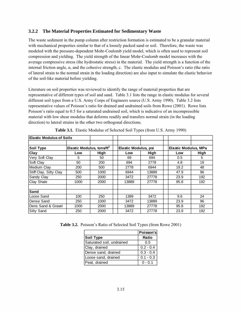
The waste sediment in the pump column after restriction formation is estimated to be a granular material with mechanical properties similar to that of a loosely packed sand or soil. Therefore, the waste was modeled with the pressure-dependent Mohr-Coulomb yield model, which is often used to represent soil compression and yielding. The yield strength of the linear Mohr-Coulomb model increases with the average compressive stress (the hydrostatic stress) in the material. The yield strength is a function of the internal friction angle, α, and the cohesive strength, c. The elastic modulus and Poisson’s ratio (the ratio of lateral strain to the normal strain in the loading direction) are also input to simulate the elastic behavior of the soil-like material before yielding. Literature on soil properties was reviewed to identify the range of material properties that are representative of different types of soil and sand. Table 3.1 lists the range in elastic modulus for several different soil types from a U.S. Army Corps of Engineers source (U.S. Army 1990). Table 3.2 lists representative values of Poisson’s ratio for drained and undrained soils from Rowe (2001). Rowe lists Poisson’s ratio equal to 0.5 for a saturated undrained soil, which is indicative of an incompressible material with low shear modulus that deforms readily and transfers normal strain (in the loading direction) to lateral strains in the other two orthogonal directions.

Table 3.1. Elastic Modulus of Selected Soil Types (from U.S. Army 1990)

Elastic Modulus of Soils

Soil TypeClay Low High Low High Low HighVery Soft Clay 5 50 69 694 0.5 5Soft Clay 50 200 694 2778 4.8 19Medium Clay 200 500 2778 6944 19.2 48Stiff Clay, Silty Clay 500 1000 6944 13889 47.9 96Sandy Clay 250 2000 3472 27778 23.9 192Clay Shale 1000 2000 13889 27778 95.8 192

SandLoose Sand 100 250 1389 3472 9.6 24Dense Sand 250 1000 3472 13889 23.9 96Dens Sand & Gravel 1000 2000 13889 27778 95.8 192Silty Sand 250 2000 3472 27778 23.9 192

Elastic Modulus, tons/ft2 Elastic Modulus, MPaElastic Modulus, psi

Table 3.2. Poisson’s Ratio of Selected Soil Types (from Rowe 2001)

Poisson'sRatio

0.50.2 - 0.40.3 - 0.40.1 - 0.30 - 0.1

Dense sand, drainedLoose sand, drainedPeat, drained

Soil TypeSaturated soil, undrainedClay, drained

3.16

However, the Poisson’s ratio can only approach 0.5 in the elastic-plastic finite element model because 0.5 gives infinite stiffness terms (i.e., full incompressibility). The elastic-plastic solution calculates the elastic portion of the total strain, assuming the material is slightly compressible. When the equivalent stress exceeds the yield stress, then the plastic strains are calculated, assuming incompressible deformation (Poisson’s ratio equal to 0.5) dominated by shearing action. Therefore, the waste-yielding model was run with Poisson’s ratios ranging from 0.4 to 0.45 to approximate the waste as a readily deformable material with low shear modulus but a high bulk modulus. Additional calculations were made with a lower Poisson’s ratio of 0.24 that is more representative of drained soils. Table 3.3 lists representative friction angles for a selection of different soil types from Day (2001). The waste cohesive strength was assumed to be 2080 Pa, which is the equivalent tensile stress that corresponds to the estimated waste shear strength of 1200 Pa (assuming von Mises yielding). The cohesive strength, c, is the tensile strength at zero hydrostatic stress. Additional calculations were made with cohesive strength equal to 6895 Pa (1 psi).

Table 3.3. Internal Friction Angle for a Selection of Soil Types (from Day 2001)

Typical Soil Friction AngleEffective Friction Angles at peak strength Effective Friction Angle

at Ultimate StrengthSoil Type Low High Low High Low HighSilt (nonplastic) 28 32 30 34 26 30Uniform Fine to medium Sand 30 34 32 36 26 30Well-Graded Sand 34 40 38 46 30 34Sand & Gravel Mix 36 42 40 48 32 36

Medium Dense

3.2.3 Case 1, Failure of Waste in the Pump Column Only

Figure 3.10 shows the two-dimensional, axi-symmetric model of the Case 1 conditions where the sedimentary waste is assumed to exist only in the pump column. Note that the X-axis is shown as the vertical axis and is the centerline axis of the pump. The Y-axis is shown horizontally to the left and is the radial axis of the axi-symmetric model. In this convention, the pump centerline is the right vertical boundary of the model. The pump inlet slot is on the lower left side of Figure 3.10. The waste is modeled as a compressible yielding material, while the pump column and the standoff ring are modeled as rigid line boundaries. The bottom view in Figure 3.10 shows the very fine numerical mesh that was used to better simulate the extrusion of waste through the narrow slot between the pump column and the standoff ring. The mesh was generated with an automatic mesh generator that first defines the mesh divisions on the boundary and then fills in the internal elements. The mesh transitions to a coarser element size as it moves away from the pump inlet slot. The model was loaded by displacing the top surface of the waste column downward while monitoring the applied pressure to check for yielding and eventual failure of the waste column to support additional load. Frictionless contact was defined between the waste and the rigid pump boundary so that the model predicts only the flow resistance provided by the waste column itself.

3.17

Figure 3.10. The Case 1 Finite Element Model of the Waste Filling the Bottom Section of the S-102

Pump Column

3.18

The model was run with the four different material data sets listed in Table 3.4. Cases 1.1 and 1.2 use low elastic moduli and higher Poisson’s ratios that are representative of the saturated waste sediment in the pump. Cases 1.3 through 1.4 were run to compare the yielding of drained soils with Poisson’s ratio equal to 0.24 and elastic moduli of 25,000 psi and 3,000 psi. The compressive displacement load was incremented to the point where the models failed to numerically converge.

Table 3.4. Input Data for Cases 1.1 Though 1.4 of the Waste Yielding Model

S-102 Pump Plugging Model, Case 1Waste Mechanical Properties

Shear Bulk Friction Shear Linear Mohr-Coulomb Parameters Final PressureCase E Poissons Mod, psi Mod, psi Angle Cohesion Cohesion Strength Sigma Sigma at nonconvergenceNo. psi Ratio psi psi degrees psi Pa Pa alpha psi Pa Mpa psi1.1 1000 0.45 345 3333 26 0.302 2079 1200 0.142 0.455 3138 1.32 1911.2 1000 0.40 357 1667 30 0.302 2079 1200 0.160 0.435 2996 1.12 1621.3 25000 0.24 10081 16026 35 1 6895 3981 0.181 1.347 9287 2.06 2991.4 3000 0.24 1210 1923 30 1 6895 3981 0.160 1.441 9937 2.05 297

Often the point of non-convergence is indicative of the failure point where the material is not able to support additional load. Although the final pressure can also be sensitive to the numerical convergence and contact convergence tolerances used, the collective trends of Cases 1.1 through 1.4 provide insight regarding the capability of a soil-like waste material to support load in the base of the pump column. Figure 3.11 is a contour plot of the pressure distribution (mean normal stress) in the waste for Case 1.1, showing high pressure inside the pump (with high yield stress) and lower pressure in the pump slot. Figure 3.12 is the corresponding shear stress distribution that shows high shear gradients in the inlet to the pump slot. Figure 3.11 and Figure 3.12 also show the final deformed shape of the waste in Case 1.1, with the waste beginning to extrude from the pump inlet slot. Cases 1.2, 1.3, and 1.4 showed similar waste extrusion near the point where the solution stopped. Figure 3.13 shows the pressure versus displacement histories for the four different cases. The maximum pressures vary considerably, depending on the assumed waste properties. Cases 1.1 and 1.2 with the saturated soil properties show final pressures of 1.1 to 1.3 MPa (160 to 190 psi). Cases 1.3 and 1.4 with the drained soil properties achieved higher pressures of about 2 MPa (290 psi). The steeper slope of Case 1.3 is consistent with the higher elastic modulus that was used. These results suggest that a column of granular waste could withstand a relatively high pressure before yielding and flow occurred. The essentially linear slopes of the pressure-displacement curves in Figure 3.13 suggest that the pressure would continue to build, compressing and locking the waste particles tighter together, until the pressure was high enough to overcome the compressive strength of the waste in the region of the pump inlet where the yield strength was low due to the correspondingly low hydrostatic pressure.

3.19

Figure 3.11. Contour Plot of the Pressure Distribution (mean normal stress) in the Waste as it Extrudes

from the Pump Inlet Slot: Case 1.1

Figure 3.12. Contour Plot of the Shear Stress Distribution in the Waste as it Extrudes from the Pump

Inlet Slot: Case 1.1

3.20

Pump Waste Yielding Prediction for a Range of Soil-Like Properties

0

0.5

1

1.5

2

2.5

0 5 10 15 20 25Displacement of Waste in Pump Column, mm

Pre

ssur

e (M

Pa)

Case 1.1

Case 1.2

Case 1.3

Case 1.4

Figure 3.13. Pressure Versus Compressive Displacement of the Waste Column

3.2.4 Case 2, Failure of Waste in the Pump Column with a Waste-Filled Annulus Around the Pump

Figure 3.14 shows the Case 2 model where the sedimentary waste is assumed to fill the bottom of the pump column plus a confined annulus around the outside of the pump. The finite-element mesh of the waste inside the pump was identical to the model for Case 1. This was done to eliminate mesh refinement issues from affecting the onset of yielding of the waste column inside the pump. The waste outside the pump was extended to a height of 4.2 inches, which is above the diameter change in the pump column. A hydrostatic pressure load equivalent to the remainder of the waste depth (see Figure 3.13) was included to simulate the effect of waste filling the 18-inch depth of the annulus around the pump. The material data input to the model were the same as used in Cases 1.1 and 1.2. These data are listed in Table 3.5.

Table 3.5. Input Data for Cases 2.1 and 2.2 of the Waste Yielding Model

S-102 Pump Plugging Model, Case 2Waste Mechanical Properties

Shear Bulk Friction Shear Linear Mohr-Coulomb Parameters Final PressureCase E Poissons Mod, psi Mod, psi Angle Cohesion Cohesion Strength Sigma Sigma at nonconvergenceNo. psi Ratio psi psi degrees psi Pa Pa alpha psi Pa Mpa psi2.1 1000 0.45 345 3333 26 0.302 2079 1200 0.142 0.455 3138 2.27 3292.2 1000 0.40 357 1667 30 0.302 2079 1200 0.160 0.435 2996 2.85 413

3.21

Figure 3.14. The Case 2 Model of Waste in the Pump Column with Waste Filling an Annulus Around

the Pump

3.22

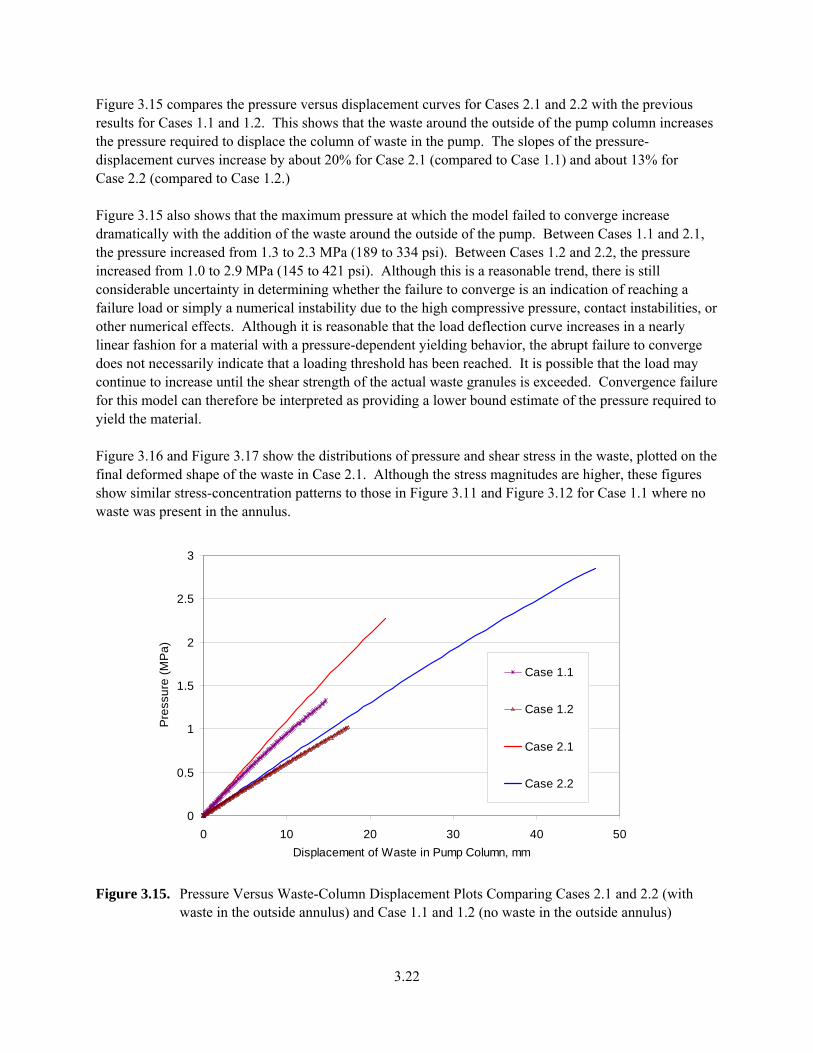
Figure 3.15 compares the pressure versus displacement curves for Cases 2.1 and 2.2 with the previous results for Cases 1.1 and 1.2. This shows that the waste around the outside of the pump column increases the pressure required to displace the column of waste in the pump. The slopes of the pressure-displacement curves increase by about 20% for Case 2.1 (compared to Case 1.1) and about 13% for Case 2.2 (compared to Case 1.2.) Figure 3.15 also shows that the maximum pressure at which the model failed to converge increase dramatically with the addition of the waste around the outside of the pump. Between Cases 1.1 and 2.1, the pressure increased from 1.3 to 2.3 MPa (189 to 334 psi). Between Cases 1.2 and 2.2, the pressure increased from 1.0 to 2.9 MPa (145 to 421 psi). Although this is a reasonable trend, there is still considerable uncertainty in determining whether the failure to converge is an indication of reaching a failure load or simply a numerical instability due to the high compressive pressure, contact instabilities, or other numerical effects. Although it is reasonable that the load deflection curve increases in a nearly linear fashion for a material with a pressure-dependent yielding behavior, the abrupt failure to converge does not necessarily indicate that a loading threshold has been reached. It is possible that the load may continue to increase until the shear strength of the actual waste granules is exceeded. Convergence failure for this model can therefore be interpreted as providing a lower bound estimate of the pressure required to yield the material. Figure 3.16 and Figure 3.17 show the distributions of pressure and shear stress in the waste, plotted on the final deformed shape of the waste in Case 2.1. Although the stress magnitudes are higher, these figures show similar stress-concentration patterns to those in Figure 3.11 and Figure 3.12 for Case 1.1 where no waste was present in the annulus.

0

0.5

1

1.5

2

2.5

3

0 10 20 30 40 50Displacement of Waste in Pump Column, mm

Pres

sure

(MP

a)

Case 1.1

Case 1.2

Case 2.1

Case 2.2

Figure 3.15. Pressure Versus Waste-Column Displacement Plots Comparing Cases 2.1 and 2.2 (with

waste in the outside annulus) and Case 1.1 and 1.2 (no waste in the outside annulus)

3.23

Figure 3.16. The Final Deformed Shape of Sensitivity Case 2.1 Showing the Distribution of Pressure

(mean normal stress) in the Waste as it Extrudes from the Pump Inlet Slot into the Annulus Around the Pump

Figure 3.17. The Shear Stress Distribution for Case 2.1 Showing the Waste Being Extruded from the Pump Slot Upward into the Annulus Around the Pump

3.24

3.2.5 Case 3, Failure of Waste in the Pump Column with a Continuous Waste Mass Around the Pump

Figure 3.18 shows the Case 3 model with sedimentary waste filling the bottom of the pump column and a large continuous waste mass surrounding the pump. The Case 3 model was generated by extending the outer boundary of the Case 2 model to a radius of 0.35 meters (13.9 inches). The material input data for Cases 3.1 and 3.2 are listed in Table 3.6.

Table 3.6. Input Data for Cases 3.1 and 3.2 of the Waste Yielding Model

S-102 Pump Plugging Model, Case 3Waste Mechanical Properties

Shear Bulk Friction Shear Linear Mohr-Coulomb Parameters Final PressureCase E Poissons Mod, psi Mod, psi Angle Cohesion Cohesion Strength Sigma Sigma at nonconvergenceNo. psi Ratio psi psi degrees psi Pa Pa alpha psi Pa Mpa psi3.1 1000 0.45 345 3333 26 0.302 2079 1200 0.142 0.455 3138 2.4 3483.2 1000 0.40 357 1667 30 0.302 2079 1200 0.160 0.435 2996 2.65 384

Figure 3.19 shows the pressure-versus-displacement plots of Cases 3.1 and 3.2 compared to those of Cases 1.1, 1.2, 2.1, and 2.2. Figure 3.19 shows that a greater expanse of waste outside the pump provides the same resistance to waste yielding as the 50-mm (2-inch) annulus around the pump column in Case 2. This seems reasonable, since the extrusion of waste through the inlet slot is a local yielding phenomenon. Figure 3.20 and Figure 3.21 show the pressure and shear stress distributions one the deformed shape of the waste model at the last converged steps of the Case 3.1. These results are similar to the Case 2 results (Figure 3.16 and Figure 3.17) except that the waste level rise is less due to the larger volume outside of the pump.

3.25

Figure 3.18. The Case 3 Model of Waste in the Pump Column with a Large Waste Mass Surrounding

the Pump. The waste extends to a radius of 0.35 m (13.9 inches).

0

0.5

1

1.5

2

2.5

3

0 10 20 30 40 50Displacement of Waste in Pump Column, mm

Pre

ssur

e (M

Pa)

Case 1.1

Case 1.2

Case 2.1

Case 2.2

Case 3.1

Case 3.2

Figure 3.19. Pressure Versus Waste Column Displacement Plots Comparing Cases 3.1 and 3.2 (a large

diameter mass of waste outside the pump) with Cases 2.1 and 2.2 (2-inch waste filled annulus) and Case 1.7 and 1.8 (no waste outside the pump)

3.26

Figure 3.20. The Final Pressure Distribution (mean normal stress) in Case 3.1 as the Waste Extrudes

from the Pump Inlet Slot Upward into the Large Waste Mass Around the Pump

Figure 3.21. The Final Shear Stress Distribution in Case 3.1

3.27

3.2.6 Additional Cases with Reduced Waste Height and Applied Pressure Loading

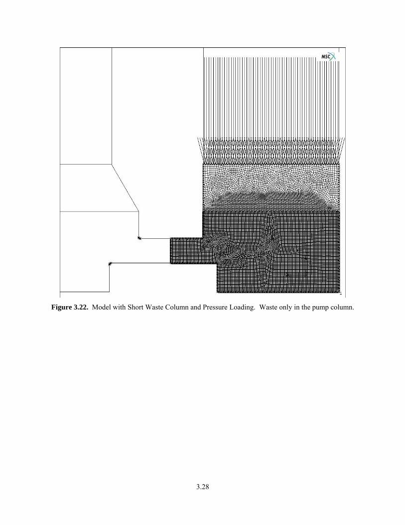
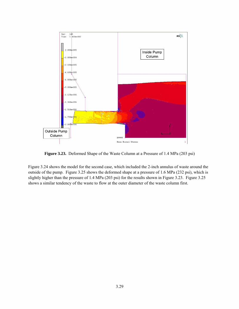
Since the dilution line failed under conditions where the column of sediment in the pump was probably relatively short, two additional sensitivity cases were developed to evaluate the differences in waste response for this condition. In these two cases, the height of the sediment layer within the pump was assumed to be 2.8 inches, corresponding to about two-thirds of the pump inlet chamber height below the stator. In the first case, the conditions outside the pump column were modeled with no waste present, a bounding case presenting the lowest possible external resistance to flow from the pump slot. In the second case, the model included the 2-inch wide waste-filled annulus outside the pump, as developed for the Case 2 model. The waste properties used for these cases are those of Case 1.2. Figure 3.22 shows the model for the case with waste extending only as far as the inlet slot of the pump. The sediment layer is compressed by an increasing fluid pressure, as shown in Figure 3.23 with a plot of the stress distribution for this case at a pressure of 1.4 MPa (203 psi). The shape of the waste column is the result of the beginning of preferential yielding and flow at the outer diameter of the pump column. This tendency to form a conical shape is similar to that predicted in the calculations for sediment-bed formation (refer to Section 3.1). The waste in the sediment bed begins to flow at the outer diameter of the column, which will eventually expose the dilution line port to liquid waste at the high pump pressure.

3.28

Figure 3.22. Model with Short Waste Column and Pressure Loading. Waste only in the pump column.

3.29

Figure 3.23. Deformed Shape of the Waste Column at a Pressure of 1.4 MPa (203 psi)

Figure 3.24 shows the model for the second case, which included the 2-inch annulus of waste around the outside of the pump. Figure 3.25 shows the deformed shape at a pressure of 1.6 MPa (232 psi), which is slightly higher than the pressure of 1.4 MPa (203 psi) for the results shown in Figure 3.23. Figure 3.25 shows a similar tendency of the waste to flow at the outer diameter of the waste column first.

3.30

Figure 3.24. Model with Short Waste Column and Pressure Loading. Waste included in 2-inch annulus

outside the pump.

Figure 3.25. Deformed Shape of the Waste Column at a Pressure of 1.6 MPa (232 psi)

3.31

3.2.7 Restriction Failure Discussion

Finite-element models were constructed to estimate the pump pressures that could be resisted by a column of granular waste in the bottom of the S-102 pump. The models used soil-like properties to simulate the estimated pressure-dependent yielding of the sedimentary waste. The results suggest that it is reasonable that pressures of 1 to 2.9 MPa (145 to 421 psi) could be resisted before the restriction would yield and flow could be initiated from the pump inlet slots. If the column of waste exists only inside the pump, then the predicted yielding pressure would be on the lower end of this range (1 to 2 MPa, 145 to 290 psi). If waste also fills the annulus outside the pump, then the predicted yield pressure is at the upper end of this range (2 to 2.9 MPa, 290 to 421 psi). Two different waste configurations were simulated. One assumed a tall column of waste loaded with an increasing compressive displacement, and the other assumed a short column of waste loaded by an increasing hydrostatic pressure. The deformed shape of the shorter waste column suggests that the material at the outer diameter of the waste column will initiate flow, creating a cone-like heel in the bottom of the pump that would tend to preferentially expose the dilution ports to liquid waste at the high pump pressure.

3.3 Restriction Flow

The TEMPEST finite-volume CFD computer code was used to estimate the pressure-time history of the S-102 pump after the restriction bed begins to fail, as calculated with the Marc finite difference code (see Section 3.2 above). The code used for this study is version T2.11, mod d (Eyler et al. 1993). This version of TEMPEST is specifically designed to address the unique properties of wastes that are contained in both single-shell and double-shell Hanford waste tanks. The code can be used to compute the three-dimensional time-dependent flow field and associated material distribution and dilution of viscous sludge and slurries.

3.3.1 Test Cases

TEMPEST (version T2.11d) calculations of fluid dynamic pressures were compared to known analytical and empirical results for smooth pipe with a cylindrical cross-section. TEMPEST results are in good agreement with analytical solutions and empirical models for all aspects of non-turbulent channel flow, including pressure drop, fully developed centerline velocity, and entrance length. The results of these test cases are presented in Appendix C.

3.3.2 TEMPEST Simulation Models

Figure 3.26 illustrates the pump-discharge geometry used in the TEMPEST model for each of the simulated cases. This figure shows a two-dimensional, axi-symmetric slice of the modeled domain. Case 0, assuming water only in the system, provides a hydrodynamic base case, for comparison to the behavior with waste in the three configurations assumed for Cases 1, 2, and 3, as presented in Section 2 above. Figure 3.27 shows the TEMPEST finite volume grid layout for Case 1, with waste in the pump and water in the exterior 2-inch annulus. Figure 3.28 shows the layout for Case 2, with waste in the pump and the

3.32

annulus. The grid layout for Case 3, assuming that the waste domain outside the pump is not constrained to the annulus, is shown in Figure 3.29.

5.0"

0.53

1"

2.953"

0.50

0"

1.20

"

2.0"

was

te

18"

V

Waste Pump: S-102

1.09375"gap flow

4.953"

0.15"

2.64"

4.20"

R = Pump Housing

0.625"

Annulus

Tank BottomPlate

out flowInflow Boundary

Cen

terli

neC L

Tank

Wal

l

Radius, Tank Wall = 37.5 ft

3.21

87"

Case 0

Base Case - Water Only

Figure 3.26. System Geometry Modeled in TEMPEST for all Cases Simulated

3.33

3

2

1

45

67

89

10

11

12

13

14

15

16

17

181920

21

22

23

solid, waste boundary Case 1

outflow

inflow velocity, Vwater

Pump Housing

waste

Plate

waste

Computatonal Cell Indices

CL

water

Annulus

1 2 3 4 5 10 15 20 25 30 35

Slurry

Tank Bottom

Figure 3.27. TEMPEST Noding Grid Overlaid on Assumed Waste Distribution for Case 1—Settled

Waste in Pump, Water in Annulus

3.34

3

2

1

45

67

89

10

11

12

13

14

15

16

17

181920

21

22

23

solid, waste boundary Case 2

water

Pump Housing

waste

Plate

slurry

waste

Computatonal Cell Indices

CL

Annulus

waste

out flow

1 2 3 4 5 10 15 20 25 30 35

inflow velocity, V

Tank Bottom

Figure 3.28. TEMPEST Noding Grid Overlaid on Assumed Waste Distribution for Case 2—Settled

Waste in Pump and Annulus

3.35

1 2 3 4 5 10 15 20 25 30 35

3

2

1

45

67

89

10

11

12

13

14

15

16

17

18

20

21

22

23 water

Pump Housing

waste

Plate

slurry

Computatonal Cell Indices

CL

5554

Tank Bottom

waste

36 - 53

19

water

Pump Housing

waste

Plate

slurry

CL waste

out flow

10

Tank

Wal

l

inflow velocity, V

Tank Bottom

Figure 3.29. TEMPEST Noding Grid Overlaid on Assumed Waste Distribution for Case 3—Settled

Waste in Pump, External Waste Domain Extending to Edge of Tank

3.3.3 Simulation Parameters

Physical-property parameters, from Section 2, used in the TEMPEST simulations are as follows: 1. Particles: Two particle sizes and particle densities were used: a. Large (<20 μ, 16%, ρ = 2.2 g/mL) b. Small (20 to 200 μ, 84%, ρ = 1.9 g/mL) c. Waste is assumed fully packed solids at 0.54% 2. Density, ρ a. Water, ρ = 62.43 lbm/ft3 b. Slurry, sg = 1.08, ρ = 67.42 lbm/ft3 c. Waste. sg = 1.51, ρ = 94.27 lbm/ft3 3. Dynamic viscosity, μ a. Water, μ = 4.7×10-4 lbm/ft-sec b. Waste and Slurry viscosity is given by the following equation:

μ = 0.002 1 + 2.5Cv +10.5Cv2 +1.3 exp 17Cv( )−1( )[ ] γ−0.06 Pa-s

3.36

4. Waste yield stress, τ0

τ0 = 1,200 Pa = 0.174 psi

3.3.4 Pressure Calculations

Table 3.7 and Table 3.8 summarize the results of the TEMPEST calculations assuming a flow of 20 gpm and 30 gpm, respectively, showing the pumping pressure over time and starting from the point of failure of the bed restriction (as determined from the calculations with the Marc finite element code; see Section 3.2). The flow rate of "normal" reverse flow of the transfer pump is nominally 130 gpm (Section 2.1), and the flow rate during the apparent over-pressurization of the dilution line is unknown. As pressure drop increases with flow rate, 20 gpm was chosen to illustrate that relatively large pressure can be developed at low (in comparison to normal operation) flow rates. The pressures developed at 20 gpm are on the same order of magnitude as the results from restriction formation and failure, Sections 3.1 and 3.2. The 50% increase to 30 gpm illustrates flow rate functionality. Case 0 is the baseline pressure simulation with pure water, which shows that for unobstructed flow, the pressure drop through the pump is quite low. Note that in Figure 3.12, the pressure is also reported at 0.1 second.

Table 3.7. Pump Pressure Time History: 20 gpm

Time, sec Case 0: H2O Case 1 Case 2 Case 3 Cumulative psi psi psi psi Gallons

0.5 1,638 2,100 1,826 0.167 1.0 32.8 371 102 0.33 5.0 6.8 134 4.54 1.67

10.0 2.2 49 1.73 3.33 20.0 0.68 6.2 0.94 6.67 30.0 0.407 0.9 0.73 10.00

Steady flow 0.212

Table 3.8. Pump Pressure Time History: 30 gpm

Time, sec Case 0: H2O Case 1 Case 2 Case 3 Cumulative psi psi psi psi Gallons

0.1 2,651 3,540 3,176 0.125 0.5 473 370 298 0.25 1.0 44 10.2 33.1 0.5 5.0 1.8 0.96 3.1 2.5

10.0 0.46 0.527 1.72 5.0 20.0 0.365 0.573 0.99 10.0 30.0 0.348 0.54 0.53 15.0

Steady flow 0.25

3.37

3.3.5 Restriction Flow Discussion

Pressure as a function of time was computed with TEMPEST for two different pump discharge rates, 20 gpm and 30 gpm, for three different initial waste configurations in the pump inlet chamber, inlet slot, and external region around the pump column. Table 3.7 and Table 3.8 summarize the pumping-pressure time-history calculations. Case 0 is the baseline pressure simulation of pure water. In each case, except for the reference Case 0, which is simply the baseline pressure simulation of pure water, the simulation shows a very high start-up pressure. This pressure spike is caused by the “instantaneous” discharge start-up. That is, the calculations do not assume a finite time for “ramp-up” of the pump discharge flow. Inertia and yield strength of the waste are responsible for this initial pressure spike. In reality, the start-up pressure would be smaller because of the small but finite time required to initiate motion of the pump rotor (in the actual event, it is expected that the pump rotor was already in motion at the time the restriction began to flow), but even so, this pressure is expected to be quite high, as the pump rotor starts up in a manner very close to a step function. An instantaneous start-up therefore provides an estimate of the upper bound on the start-up pressure. After the first half second of the transient, the effects of the instantaneous start-up have essentially dissipated, and in all cases with a 20-gpm flow rate, shown in Table 3.7, the predicted pressure response is the result of overcoming the waste viscosity. The initial inventory of stagnant waste in the pump inlet chamber is mostly cleared out in 30 seconds, which is the time required for approximately 10 gallons of water to flush the system, although some solid particles remain on the floor and in low-flow areas. In the calculations with 30 gpm, shown in Table 3.8, the waste is essentially cleared out of the system in about 20 seconds. Note that the initial pressure spike is larger in the 30-gpm simulations but deceases more rapidly with time than for the 20-gpm cases. This is because the yield strength is overcome more rapidly, and the particles are cleared out of the system faster at the higher flow rate. In Case 1 (see Figure 3.29), water is assumed to fill the annulus initially, and the pressure drops off rapidly as the system is rapidly flushed of particles. In Case 2, the annulus is assumed to be filled with fully packed waste. In this case, the process of flushing waste out of the annulus causes the pressure to remain high for several seconds. In addition, there appears to be some slight pressure oscillation after about 20 seconds in the 30-gpm cases. In Case 3, there is no assumption that the waste external to the pump is confined within a restrictive annulus. The waste extends from the pump to the tank wall at an 18-inch depth. The tank wall is set at a radius of 37.5 feet. In this case, the waste and slurry flow emanates from the slot gap as an eroding jet. This flow easily erodes a pathway into the surrounding waste, forming a diluting, buoyant plume. Again, the resulting pressure quickly decreases, as shown in Table 3.7 and Table 3.8 for both assumed flow rates. For Cases 2 and 3, the TEMPEST results show that for the first 1 to 5 seconds of flow, the pressure in the pump reaches 100 to 370 psi. In all cases, the final pressure approaches that of the pressure required to flow pure water through the system as particles are cleared out of the pump chamber and surrounding external annulus.

4.1

4.0 Summary

The results of the sediment-bed formation, failure, and flow simulations provide insights into the over-pressurization and failure of the S-102 dilution water-supply hose while operating the retrieval pump in reverse. All software used for the simulations is identified as “non-safety software” in that results provided from the software models are not to be used in any nuclear-safety-related manner for design, monitoring, and/or administrative functions of a nuclear facility. The results do not ensure the proper accident or hazards analysis of a nuclear facility or an SSC that performs a safety function. The purpose of this work was to identify plausible scenarios; all results must be treated as qualitative. The three modeling cases presented in Section 2.4 were evaluated. Case 1 represents the least-restrictive condition possible in that resistance to flow will only be developed by the slurry in the pump column. In Case 2, the restriction is formed by the slurry in the pump column flowing into an external restriction constrained annularly by a fixed boundary. Case 3 differs from Case 2 in that the annular fixed boundary is replaced with sludge, removing the fixed radial constraint on the reverse flow. As presented in Section 3, three software models were employed for each case to evaluate the pressure at the dilution-line inlet during sediment-bed restriction formation, failure, and flow, respectively. The restriction formation was modeled using the lattice Boltzmann method, the restriction failure was modeled using the Marc finite element code, and the restriction flow was modeled using the TEMPEST finite-volume CFD code. Results for the pressure at the dilution-line inlet are summarized in Table 4.1. The flow conditions are presented as a function of time starting at 1 sec to remove the pressure spike caused by the “instantaneous” discharge start-up. For Case 1, the restriction failure pressure is lower than the formation pressure, indicating that the sediment bed would fail and flow would be initiated prior to the attained formation pressures, and the pressure is even lower for the flow conditions. The failure pressure range is greater than the formation pressure for Cases 2 and 3, indicating that the restriction was capable of withstanding an increased pressure after the pump inlet cavity was filled (see Section 3.1). After initiation of flow at 20 gpm, the pressure for Case 2 at 1 second is similar in magnitude to that of restriction failure. For both restriction formation and flow, the Case 3 results are decreased in comparison to Case 2 due to the removal of the annular boundary that restricts the flow. The sediment-bed-formation model predicts that the pump inlet can accumulate a significant restriction resulting in pressures at the dilution line inlet of 200 to 300 psi. After the major deposition event occurred to form the restriction, the continuing and subsequent periods of reverse pump operation could have provided the small amount of waste necessary to completely restrict the inlet. The failure model confirms that once the sediment bed was formed, it was probably strong enough that pressures of 300 to 400 psi would be required to backflow the restriction material out of the inlet slots. Finally, the flow model shows that high initial pressures (100 to 370 psi) would be required during the initiation of reverse flow of the restriction.

4.2

Table 4.1. Pressure Results at Dilution Line Inlet

Pressure (psi) Failure Flow Formation

.1(a) .2(a) Time (s) 20 gpm 30 gpm 1 33 44 Case 1 290 191 162

10 2.2 0.5 1 371 10.2 Case 2 235 329 413

10 49 0.5 1 102 33 Case 3 195 348 384

10 1.7 1.7 (a) Refers to Case numbers—see Section 3.2.

5.1

5.0 References

Callaway WS. 2003. Tank 241-S-102 Core Sample Dissolution Testing Report. RPP-15940, Rev. 0, CH2M HILL Hanford Group, Richland, WA. CH2M HILL Hanford Group. 2007. Root Cause Analysis Report, CH2M-HIL-PER-2007-1327, Radioactive Waste Spill at 241-S-102 on July 27, 2007. RPP-RPT-34831, Richland, WA. Day RW. 2001. Soil Testing Manual. ISBN 0-07-136363-7. McGraw-Hill, Inc., New York, NY. Eyler LL, DS Trent, and J A Fort. 1993. TEMPEST, A Computer Program for Three-Dimensional, Time-Dependent Computational Fluid Dynamics. Volume 2: Users Manual. Version T2.11d. PNL-8857, Vol. 2, Rev. 1, Pacific Northwest Laboratories, Richland, WA. Jewett JR, SD Estey, L Jensen, NW Kirch, DA Reynolds, and Y Onishi. 2002. Values of Particle Size, Particle Density, and Slurry Viscosity to Use in Waste Feed Delivery Transfer System Analysis. RPP-9805, Rev. 1, Office of River Protection, Richland, WA. Rowe RK. 2001. Geotechnical and Geoenvironmental Engineering Handbook. R. K. Rowe, Editor. Springer-Verlag, New York, NY. Sukop MC and DT Thorne, Jr. 2006. Lattice Boltzmann Modeling: An Introduction for Geoscientists and Engineers. Springer-Verlag Press, Berlin. U.S. Army. 1990. Engineering and Design, Settlement Analysis. CECW-EG, Engineering Manual, 1110-0-1904. Department of the Army, U.S. Army Corps of Engineers, Washington, D.C. Wells BE, MA Knight, EC Buck, SK Cooley, RC Daniel, LA Mahoney, PA Meyer, AP Poloski, JM Tingey, WS Callaway III, GA Cooke, ME Johnson, MG Thien, DJ Washenfelder, JJ Davis, MN Hall, GL Smith, SL Thomson, and Y Onishi. 2007. Estimate of Hanford Waste Insoluble Solid Particle Size and Density Distribution. PNWD-3824, WTP-RPT-153, Rev. 0, Battelle-Pacific Northwest Division, Richland, WA. Wilcox DC. 1993. Turbulence Modeling for CFD. DCW Industries, La Canada, CA.

A.1

Appendix A: Test Cases for Sediment Formation

Two validation cases were completed with the Pacific Northwest National Laboratory lattice kinetics computer program used to model the pump sediment formation. The first case modeled turbulent flow through a slit channel. The channel is 12.7 cm (5 in.) wide and 35.3 cm (~14 in.) long and modeled using a 38×100 grid. This test case is similar to a classic experiment performed by Laufer (1951), which is extensively referenced in the literature. Air at room temperature flows through the channel with an average velocity of 300 cm/s. A transient simulation was performed until steady-state conditions were achieved. The transverse velocity profile, shown in Figure A.1, is compared to the log law profile, given by the approximate expression

u+ =u

τ w ρ=

1κ

lnn+ + B (A.1)

where κ is the von Karmen constant, 0.41, and B is the intercept, 5.5 (Wilcox 1993). The log law profile is not expected to be accurate near the centerline since the velocity gradient must approach zero. The velocities are within 7% at all locations. The difference near the wall is due to the use of boundary wall functions, which use an approximate method for integrating the combined contributions of the viscous sublayer and the turbulent region. The pressure gradient along the channel given by the simulation is approximately 4.50e-2 g/cm2-s2. The friction factor, Λ, for a parallel channel is given by the implicit expression (White 1991)

1

Λ0.5 = 2.0log10(ReDhΛ0.5) −1.19 (A.2)

Using this value, the pressure gradient is calculated to be 4.36e-2 g/cm2-s2, which is within 4% of the simulation result. The second case was a growing sediment bed in a slit channel. A particle suspension flows through a stationary bed and deposits the solid material. The bed has a specified flow resistance that is a function of solids concentration. As the bed grows, the total pressure drop in the channel increases as a function of time. The sediment model is described in more detail in Section 3.1.1. The channel is 2 cm wide and 10 cm long and modeled using a 22×100 grid. The sediment is assumed to consist of 100 micron particles packed to 54 vol%. The fluid consists of 1 vol% suspended particles in a liquid with a base viscosity of 0.01 g/cm-s. The simulation begins with the last 0.5 cm of the channel filled with sediment. The suspension flow rate is set at 2 cm/s. The sediment length as a function of time is shown in Figure A.2, and the pressure drop as a function of time is shown in Figure A.3. In the first 100 seconds, over 40% of the channel is filled. The Darcy

A.2

resistance is calculated using the Ergun equation described in Section 3.1.1. The pressure drop rises linearly as the sediment bed depth increases. These test cases demonstrate that the turbulent model, important for cycle 1 of Case 1, and the sediment growth and resistance model, important for the other cases, give reasonable results.

Figure A.1. Velocity Profile for Turbulent Flow in Slit Channel

Figure A.2. Sediment Length as a Function of Time

A.3

Figure A.3. Sediment Pressure Drop as a Function of Time References Laufer J. 1951. Investigations of Turbulent Flow in a Two-Dimensional Channel. NACA Report 1053 White FM. 1991. Viscous Fluid Flow. McGraw-Hill Press, New York, NY. Wilcox DC. 1993. Turbulence Modeling for CFD. DCW Industries, La Canada, CA.

B.1

Appendix B: Validation of the Marc Finite Element Code for Simulating Sediment Yielding in the Static Pump Test

Test problems distributed with the Marc finite-element software have been executed to verify the correct solution of material models and contact conditions that will be used to simulate the initial yielding and flow of waste plugging the inlet of the positive displacement pump in Tank S-102. All calculations described below were obtained using Marc, Version 2005-R3, installed on computer WD46945 at the Pacific Northwest National Laboratory. The first test problem compares the yielding of a soil-like material. The pressure-insensitive von Mises yield criteria are compared with the pressure sensitive Mohr-Coulomb yield criteria. Example problem 3.9 from the Marc documentation simulates the yielding of a soil mass with an internal rigid cavity that is subjected to increasing pressure applied horizontally to the left vertical boundary (Figure B.1). Figure B.2 shows the global load deflection curve from the Marc manual as the material loads up and eventually yields. Figure B.3 shows the global load deflection results obtained with Marc, Version 2005-R3. Although the results are not identical, they are very close, and the current execution reproduces the same difference in yielding of the von Mises (pressure-insensitive yield stress) compared to the Mohr-Coulomb (yield stress increasing with pressure). It should be noted that the Marc example problems are intended to demonstrate the application of different material models and analysis options. The results in the manuals are not rerun for each new code release, and therefore minor differences due to improvements in numerical algorithms are to be expected between code versions. A second model was generated to further confirm the correct behavior of the Mohr-Coulomb and von-Mises yield models. This model simulated uniaxial compression and yielding of a cylindrical soil column (Figure B.4). Since the stress distribution in this problem is uniform throughout the cross-section, it should result in a sharp change in axial stiffness (the slope of the load-deflection curve) when the material yields. Figure B.5 shows that the von Mises material yields exactly at the input yield stress of 202 psi, whereas the Mohr-Coulomb material (with equivalent material properties for the pressure-sensitive yield model) has a higher yield strength (324 psi) because the mean normal stress in the soil column is compressive. This further confirms the correct behavior of this soil-like material model compared to the von Mises pressure-insensitive yield behavior. Marc example problem 8.17 simulates three-dimensional extrusion with contact and sliding against rigid die surfaces. It is important to exercise the Marc contact capability because the pump inlet model must include sliding of the waste against the pump walls as it is forced back through the pump inlet slots. The example problem 8.17 input file was rerun, and the results were compared with the published results in the Marc manual. Figures B.6 and B.7 show that the current evaluation of example 8.17 produces an equivalent stress distribution that is within 2% of the plotted results in the Marc examples manual. This is within acceptable accuracy considering that the reported results were not necessarily produced with the same version of the code or the same computer platform.

B.2

Figure B.1. Marc Example Problem 3.9. Soil with a central rigid cavity loaded by horizontal side pressure.

B.3

Figure B.2. Global Load Displacement Curves from Marc Example Problem 3.9

Marc Example Problem 3.9Mohr-Coulomb Soil Model

0

100

200

300

400

0 0.05 0.1 0.15 0.2 0.25Surface X Displacement (inch)

Surf

ace

Pres

sure

(psi

)

Von Mises Yield

Parabolic Mohr Coulomb

Figure B.3. Global Load Displacement Curves from the Comfirmatory Analysis of Marc Example Problem 3.9

B.4

Figure B.4. Axial Compression Model Used to Test the von Mises and Mohr-Coulomb Yielding Models

Uniaxial Compression, von Mises and Mohr-Coulomb Yield Models

0

50

100

150

200

250

300

350

0 0.0002 0.0004 0.0006 0.0008 0.001 0.0012 0.0014Displaements (inch)

Com

pres

sive

Stre

ss (p

si)

von Mises yieldingMohr Coulomb yielding

Yield = 202 psi

Yield = 324 psi

Figure B.5. Comparison of the Yield Thresholds for the vin Mises and Mohr-Coulomb Yielding Models

B.5

Figure B.6. Equivalent Stress Results from the Marc Manuals for Example Problem 8.17

Figure B.7. Equivalent Stress Results from the Comfirmatory Analysis of Marc Example Problem 8.17

C.1

Appendix C. TEMPEST Testing for Pressure Calculation

This appendix presents certain TEMPEST calculations of fluid dynamic pressure compared to known analytical and empirical results to establish the extent 2of the code’s accuracy in such cases. Few analytical results are available for this purpose. Testing here is for non-turbulent flow in smooth pipe with a cylindrical cross-section. Laminar flow in a Smooth Cylindrical Pipe Analytical results for laminar flow are as follows:

1. Pressure drop: ΔP = 32μU LD2

⎛ ⎝ ⎜

⎞ ⎠ ⎟

2. Entrance length: Le = 0.0575 Re

3. Velocity profile: u

umax

= 1 −rR

⎛ ⎝ ⎜

⎞ ⎠ ⎟

2

; parabolic

4. Centerline velocity: umax

U = 2; fully established flow

Nomenclature: ΔP = pressure drop, lbs/ft2 U = average flow velocity, ft/sec u = local flow velocity, ft/sec D = pipe diameter, ft R = pipe radius, ft r = radial location, ft L = pipe length, ft Le = entrance length, ft μ = dynamic viscosity, lbm/ft-sec Re = Reynolds number, ρ U D/μ Assessment of Laminar Pipe Flow Here TEMPEST results are compared to analytic and empirical pipe flow values. For the purpose of assessment, a long, smooth pipe having diameter, D = 0.5 ft, with the liquid entrance velocity, U = 1.0 ft/sec, was used. Several values of dynamic viscosity were applied in the simulation, resulting in a range of Reynolds numbers. The largest value of viscosity used in the simulations is μ ≈ 104 cp (6.72 lbm/sec-ft), estimated to be several times the viscosity of a typical Hanford sludge. Note that for these simulations, the Reynolds number may be far into the turbulent flow regime, but the analytical solution

C.2

does not assume turbulence. The assumed laminar pressure drops can be compared with TEMPEST results for large Reynolds numbers as long as the computer code is using laminar flow assumptions. This is done simply to test a large range of Reynolds numbers. Results of these tests are shown in Table C.1.

Table C.1. TEMPEST Cylindrical Pipe Laminar Flow Test Results

Viscosity, μ ΔP/L: lbf/ft2/ft umax/ U Lent: ft lbm/ft sec cp Analytic TEMPEST Analytic TEMPEST Empirical TEMPEST0.00672 10 0.796 0.834 2 1.94 160 150–160 0.0672 100 7.96 8.35 2 1.94 16.0 10–20 0.672 1000 79.6 83.5 2 1.94 1.60 ≈ 0.5(a) 6.72 10,000 796 835.0 2 1.94 0.16 ≈ 0.2(a)

(a) Difficult to estimate because of node size. As indicated by the results above, TEMPEST does a good job of predicting all aspects of non-turbulent channel flow. The maximum centerline velocity is low by about 3%. The entrance length is an asymptotic relationship. Small differences in the maximum centerline value will give a large difference in Lent. Hydrostatic pressure test Let density, ρ = 75 lbm/ft3 and height, h = 1,000 ft. Analytic result: P = ρh = 75×1000 = 75,000 lbf/ft2 TEMPEST: P = 75,005 lbf/ft

PNNL-17424

C.1

Distribution No. of Copies OFFSITE

No. of Copies ONSITE

Yasuo Onishi Consulting LLC Y. Onishi 144 Spengler St. Richland, Washington 99354

4 CH2M Hill W. B. Barton S7-90 J. E. Meacham R2-58 R. E. Raymond R2-58 M. H. Sturges S7-12

6 Pacific Northwest National Laboratory

J. M. Cuta K7-15 K. I. Johnson K5-22 D. R. Rector K7-15 D. S. Trent K7-15 B. E. Wells (2) K7-15