Research ArticleIntelligent Optimization AlgorithmsA Stochastic Closed-Loop Supply Chain Network ProblemInvolving Oligopolistic Competition for Multiproducts andTheir Product Flow Routings
Yan Zhou1 Chi Kin Chan2 Kar Hung Wong3 and Y C E Lee2
1Department of Management Science and Engineering Qingdao University Qingdao 266071 China2Department of Applied Mathematics The Hong Kong Polytechnic University Kowloon Hong Kong3School of Computational and Applied Mathematics University of the Witwatersrand Johannesburg 2050 South Africa
Correspondence should be addressed to Yan Zhou yanyanz22hotmailcom
Received 29 March 2015 Revised 20 July 2015 Accepted 26 July 2015
Academic Editor Giovanni Falsone
Copyright copy 2015 Yan Zhou et alThis is an open access article distributed under theCreative CommonsAttribution License whichpermits unrestricted use distribution and reproduction in any medium provided the original work is properly cited
Recently the first oligopolistic competitionmodel of the closed-loop supply chain network involving uncertain demand and returnhas been established This model belongs to the context of oligopolistic firms that compete noncooperatively in a Cournot-Nashframework In this paper we modify the above model in two different directions (i) For each returned product from demandmarket to firm in the reverse logistics we calculate the percentage of its optimal product flows in each individual path connectingthe demand market to the firmThis modification provides the optimal product flow routings for each product in the supply chainand increases the optimal profit of each firm at the Cournot-Nash equilibrium (ii) Our model extends the method of finding theCournot-Nash equilibrium involving smooth objective functions to problems involving nondifferentiable objective functionsThismodification caters for more real-life applications as a lot of supply chain problems involve nonsmooth functions Existence of theCournot-Nash equilibrium is established without the assumption of differentiability of the given functions Intelligent algorithmssuch as the particle swarm optimization algorithm and the genetic algorithm are applied to find the Cournot-Nash equilibrium forsuch nonsmooth problems Numerical examples are solved to illustrate the efficiency of these algorithms
1 Introduction
In the past decade the perfect competition equilibriummodels of the supply chain network (SCN) have been widelystudied For instance a perfect competition determinis-tic equilibrium model and a stochastic equilibrium modelinvolving a lot of decision-makers were first established byNagurney et al [1] and Dong et al [2] respectively On theother hand a perfect competition equilibrium model of areverse SCN was constructed by Nagurney and Toyasaki [3]for the optimal management of the electronic wastes More-over perfect competition equilibrium models of a closed-loop supply chain (CLSC) network were established byHammond and Beullens [4] andYang et al [5] for the optimalmanagement of waste electricalelectronic equipment andraw material respectively Qiang et al [6] were the first
to investigate a stochastic equilibrium model of a CLSCnetwork which involved uncertainties in demands but notuncertainties in returns The equilibrium conditions of allthe above papers were obtained by the theory of varia-tional inequality and were solved by the modified projectionmethod (Korpelevich [7])
Nowadays more firms are aware of the importance ofintegrating the supply chain as a whole consisting of all themarketing activities of all the competitors The integrationof the entire supply chain generates oligopolistic competitionamong firms As a consequence research works were recentlyextended from the perfect competition markets model to theoligopolistic firmsmodel in the forward SCNThe oligopolis-tic competition among firms in the forward SCNwas consid-ered in a lot of real-life situations For instance oligopolistic
Hindawi Publishing CorporationMathematical Problems in EngineeringVolume 2015 Article ID 918705 22 pageshttpdxdoiorg1011552015918705
2 Mathematical Problems in Engineering
competition equilibrium models of a forward SCN wereestablished by Masoumi et al [8] and Yu and Nagurney [9]for the optimal management of perishable products such aspharmacies and fresh foods and by Nagurney and Yu [10] forthe minimization of emission-generations The equilibriumconditions of these models were also obtained by the theoryof variational inequality and were solved by the Eulermethod(Dupuis and Nagurney [11])
However for both perfect competition and oligopolisticcompetition the CLSC integrating the forward and reversesupply chain ismore important than the forward supply chainalone due to the government legislation (such as the paperrecycling directive and WEEE within the European Union[12]) Moreover the process used in the CLSC to recycleused products (such as papers glass building wastes andelectronic and electrical equipment) for minimizing resourcewastage also leads to peoplersquos understanding of the greensupply chainmanagement (GSCM) (Sheu and Talley [13] andSeuring [14]) Research work on oligopolistic competitionmodel of the CLSC network only began very recently Thefirst oligopolistic competition equilibriummodel of theCLSCnetwork was established recently by Zhou et al [15]
The model developed by Zhou et al [15] belongs to thecontext of oligopolistic firms that compete noncooperativelyin a Cournot-Nash framework in a stochastic environmentSince the demands and returns are uncertain two typesof risk namely the overstocking and understocking ofmultiproducts in the forward supply chain are consideredBy using the quantities of each new product and the pathflows of each product on the forward supply chain as thedecision variables every oligopolistic firmrsquos expected profitcan be maximized at the Cournot-Nash equilibrium Theequilibrium condition of this model was also obtained by thetheory of variational inequality the variational inequalities inthis paper were solved by the logarithmic quadratic proximalprediction-correction method (He et al [16])
Asmentioned in the abstract wemodify the abovemodelin two different directions as follows
(i) Themodel of Zhou et al [15] can calculate the optimalproduct flow in each path from firms to demandmarkets in the forward logistics but not in pathsfrom demandmarkets to firms in the reverse logisticsbecause the quantity of the returned products fromeach demand market is a random variable In thispaper for each returned product 119895 from demandmarket 119877119896 to firm 119894 in the reverse logistics we cancalculate the percentage of its optimal product flowsin each individual path connecting the above demandmarket to the above firm This modification providesthe optimal product flow routings for each productin the entire supply chain and hence can increase theoptimal profit of each of the firms at the Cournot-Nash equilibrium
(ii) Our proposed model extends the method of findingthe Cournot-Nash equilibrium for CLSC problemsinvolving smooth objective functions to problemsinvolving nondifferentiable objective functions Thismodification caters for more real-life applications as
a lot of supply chain problems involve nonsmoothobjective functions
In this paper we establish the Cournot-Nash equilib-rium without the assumption of differentiability on thegiven functions and use intelligent algorithms such as thegenetic algorithm and the particle swarm optimization (PSO)algorithm for finding the Cournot-Nash equilibrium fornonsmooth CLSC problems
Genetic algorithm (Holland [17]) is a common intelligentoptimization algorithm which can find the Nash (Nash[18 19]) equilibrium effectively For instance genetic algo-rithm has been used for finding the Stackelberg- [20] Nashequilibrium of a nonlinear nonconvex nondifferentiablemultilevel programming model (Liu [21]) Complicated SNCproblems involving the design of the hierarchical spanningtree network (Kim et al [22]) and that of a vendor man-aged inventory SNC network (Yu and Huang [23]) werealso successfully solved by the genetic algorithm In thesepapers the efficiency of the genetic algorithm for solvingcomplicated combinational problems in terms of both speedand accuracy has been demonstrated
The PSO algorithm originally proposed by Eberhartand Kennedy [24] is a member of the swarm intelligencemethods (Kennedy and Eberhart [25]) for solving globaloptimization problems Similar to a lot of intelligent opti-mization algorithms the PSO algorithm does not require thegradient information of both the objective functions and theconstraint functions but only their values Thus it is easilyimplemented and computationally inexpensive and has beensuccessfully applied to solve continuous optimization prob-lems as well as discrete optimization problems (Goksal et al[26]) Numerical results have shown that the PSO algorithmis more efficient than the genetic algorithm especially forsolving problems involving continuous solution space Forinstance Kadadevaramath et al [27] and Govindan et al[28] solved respectively a three-echelon SCN problem andan optimization problem involving both the economic andenvironmental benefits of a perishable food SCN by both thegenetic algorithm and the PSO algorithm Numerical resultsindicated that the PSO algorithm is more efficient than thegenetic algorithm in terms of the accuracy of the optimalsolutions
In Section 5 of this paper two numerical examples aresolved to compare the efficiencies of the PSO algorithm thegenetic algorithm and an algorithm based on variationalinequalities for finding theCournot-Nash equilibrium In onenumerical example (Example 1) the results show that whenall the given functions are differentiable the efficiencies ofthe PSO algorithm the genetic algorithm and the algorithmbased on variational inequality are almost the same in termsof the accuracy of the computed equilibrium Howeverthe PSO algorithm is just as efficient as the algorithmbased on variational inequality but more efficient than thegenetic algorithm in terms of the total computational timerequired to obtain the equilibrium In another numericalexample (Example 2) the results show that for problemsinvolving nonsmooth objective functions the PSO algorithmand the genetic algorithm can still find the Cournot-Nash
Mathematical Problems in Engineering 3
Firm 1
1
Firm I
I
M1
1M1
n1119872
D1
1 D1
n1119863
R1 R1Rn119877Rn119877
C1
1 C1
n119862
DI
1 DI
n119863
CI
1 CI
n119862
MI
1
MI
n119872
middot middot middot
middot middot middot
middot middot middot
middot middot middot
middot middot middot
middot middot middot middot middot middot
middot middot middot
middot middot middot
middot middot middot
Demand market Demand market
Forward supply chain networkReverse supply chain network
Figure 1 The CLSC network topology
equilibrium efficiently but the algorithmbased on variationalinequality is not efficient
The rest of this paper is as follows Section 2 develops theoligopolistic CLSC network model with multiproducts anduncertain demands and returns and constructs the Cournot-Nash equilibrium conditions for our model Section 3 provesthe existence of theCournot-Nash equilibrium for ourmodelSection 4 presents a PSOalgorithmand a genetic algorithm tofind the Cournot-Nash equilibrium In Section 5 numericalexamples are solved to compare the effectiveness of the PSOalgorithm the genetic algorithm and an algorithm based onvariational inequality for finding the Cournot-Nash equilib-rium Section 6 presents our summary and conclusion
2 An Equilibrium Model of a CLSC Networkunder Oligopolistic Competition amongFirms Involving Product Flow Routings inBoth Forward and Reverse Logistics
Zhou et al [15] have established the first oligopolistic com-petition model of the closed-loop supply chain network(CLSC) involving uncertain demand and return This modelbelongs to the context of oligopolistic firms that competenoncooperatively in a Cournot-Nash framework In thismodel they maximize every oligopolistic firmrsquos expectedprofit by deciding the optimal production qualities of eachnew product as well as the amount of product flows ineach individual path containing firms to demand marketsin the forward logistics Due to the fact that the quantitiesof returned products are random variables they are unableto calculate the optimal amount of product flows in thereverse logistics In this paper we modify the above modelby including the percentage of product flows in each path inthe reverse logistics as a decision variable
The topology of the network of our model is shown inFigure 1 Each firm 119894 (119894 = 1 119868) produces 119869 products Inorder to satisfy the demand the firms eithermanufacture newproducts or remanufacture used products through recyclingused components obtained from the previous productionperiod Both the demands and returns are random variableshaving uniform distributions As mentioned in the previousparagraph each firm determines the optimal productionquantities of the new products the amount of product flowsin each path in the forward logistics and the percentage ofproduct flows in each path in the reverse logistics tomaximizeits profit
In the closed-loop supply chain each firm is representedas a network of its economic activities In the forwardlogistics firm 119894 (119894 = 1 119868) has 119899119894
119872manufacturing
facultiesplants and 119899119894119863distribution centers and serves the
same 119899119877 demand markets In the reverse logistics firm 119894
has 119899119894119862recovery centers The activities in the forward supply
chain involve the production remanufacturing deliveryand distribution of products The activities in the reversesupply chain involve the disposal recycling and returning ofproducts
In Figure 1 the links from the top-tiered 119894 (119894 = 1 119868)of the forward logistics representing the individual firm areconnected to the manufacturing nodes of the respective firm119894 which are denoted by 119872119894
1 119872119894
119899119894119872
respectively The linksfrom the manufacturing nodes are in turn connected tothe distribution center nodes of firm 119894 which are denotedby 1198631198941 119863119894
119899119894119863
respectively The links from the distributioncenters nodes are in turn connected to the demand marketnodes denoted by 1198771 119877119899119877 respectively each of thesedemand markets is served by all the firms
Also in Figure 1 the links from every demand marketnode 119877119896 (119896 = 1 119899119877) of the reverse logistics are connected
4 Mathematical Problems in Engineering
to all the recovery center nodes of firm 119894 which are denoted by1198621198941 119862119894
119899119894119862
respectively Finally the links from the recoverycenters nodes are connected to firm 119894 to complete a singleloop
Thus our CLSC network is one which incorporates theforward supply chain processes (such as production reman-ufacturing delivery and distribution) with the reverse supplychain processes (such as disposal recycling and returning) toform a closed-loop network
We wish to emphasize that the network topology inFigure 1 is for demonstration purpose only In fact the modelcan handle any prospective closed-loop chain network topol-ogy provided that there are top-tiered nodes to representeach firm and bottom-tiered nodes to represent the demandmarkets with two sequences of directed links containing eachtop-tiered node to each bottom-tiered node in the forwardand reverse directions respectively
In the forward supply chain any set of correlated linksthat can connect a firm to a demand market via a manu-facturer and a distribution center form a forward path 119901119891Similarly in the reverse supply chain any set of correlatedlinks that can connect a demand market to a firm via therecovery center form a reverse path 119901119903 From the discussionin the previous paragraph the structure of our model can becompleted specified by its forward and reverse paths
We now give a few assumptions together with theirjustifications These are common assumptions in the CLSCliterature except possibly for (A8) (See Hammond andBeullens [4] and Zhou et al [15] for details)
Assumption A (A1) The demand for product 119895 (119895 = 1 119869)of firm 119894 (119894 = 1 119868) at demand market 119877119896 (119896 = 1 119899119877)in one production period denoted by 119889119894119895119896 is a randomvariable Any two demands119889119894111989511198961 and119889119894211989521198962 with (1198941 1198951 1198961) =(1198942 1198952 1198962) are independent of each other This assumption isdue to the fact that all the buyers are independent
(A2) A fraction of the used products which is in goodcondition will be returned to the firms for remanufacturingthe remainder of used products which is not in goodcondition will be sent to the landfill for disposal Thus weassume that for any used product 119895 (119895 = 1 119869) which is ingood condition a cost of 120588Re
119895per item will be charged to the
firms for the purchase of these used products For any usedproduct 119895 (119895 = 1 119869) which is not in good condition a costof 120588 (independent of 119895) per item will be charged to the firmsfor the disposal of these used products at the landfall
(A3)All the returned products are remanufacturableThisassumption is a direct consequence of (A2)
(A4) The return of used product 119895 (119895 = 1 119869) fromdemand market 119877119896 (119896 = 1 119899119877) to firm 119894 (119894 = 1 119868) inone production period denoted by 119903119896119895119894 is a random variableAny two returns 119903119896111989511198941 and 119903119896211989521198942 with (1198961 1198951 1198941) = (1198962 1198952 1198942)are independent of each other This assumption is due to thefact that all the customers are independent
(A5) Due to the existence of modern manufacturingtechnologies manufacturers can easily transform the reman-ufactured products into as-new products Thus we assumethat there is no distinction between the qualities of the brand
new products and the remanufactured products and they aresold to the markets at the same price
(A6) The operational cost of product 119895 on any link 119886 inthe forward logistics denoted by 119888119895119886 is a continuous functionof all the link flows of this product in the forward supplychain In other words 119888119895119886 depends continuously not only onthe product flow in link 119886 but also on the product flows inall the manufacturer links and all the shipment links andall the distribution links Consequently the operation costof product 119895 on any path 119901119891 in the forward supply chaindenoted by 119888119895119901119891 is also a continuous function of all thepath flows of its product in the forward supply chain Thisassumption is due to the fact that competition for businessexists among all the companies involving economic activitiesin the forward logistics
(A7) The operational cost of product 119895 on any path 119901119903 inthe reverse logistics denoted by 119888119895119901119903 is a continuous functionof the path flow of this product on 119901119903 only
(A8) For product 119895 (119895 = 1 119869) of firm 119894 (119894 = 1 119868)the cost of manufacturing 119911 items of new product 119895 by firm 119894
is 119891119894119895(119911) and the cost of remanufacturing 119911 items of returned
product 119895 by firm 119894 is 119891Re119894119895
(119911) where 119891119894119895and 119891
Re119894119895
are givencontinuous functions Due to the operational advantages themanufacturing costs are higher than the remanufacturingcosts that is
119891119894119895(119911) gt 119891
Re119894119895
(119911) (1)
for 119894 = 1 119868 and 119895 = 1 119869(Note that due to the logistics advantages the optimal
strategies of any firm 119894 (119894 = 1 119868) at the Cournot-Nash equilibrium must automatically satisfy the followingrelationship total reverse logistics costs of firm 119894 (ie totalpurchase costs of returned products + total transportationcosts of returned products) + total remanufacturing costs offirm 119894 lt total manufacturing costs of firm 119894)
(A9) Due to the limitation of the facilities at themanufac-turersrsquo factories the quantity of new product 119895 (119895 = 1 119869)manufactured by firm 119894 (119894 = 1 119868) in one productionperiod cannot exceed 119909 where 119909 is a positive integer
In order to formulate the problemof finding theCournot-Nash equilibrium for our CLSC network we first formulatethree types of decision variables namely the quantity of newmanufactured product the amount of product flows in eachpath in the forward logistics and the percentage of productflows in each path in the reverse logistics
For any firm 119894 (119894 = 1 119868) there are 119899119894119872
manufacturersand 119899119894
119863distribution centers served for firm 119894 in the forward
logistics Thus there are altogether 119899119894119872
times 119899119894119863different paths
which can connect firm 119894 to demand market 119877119896 (119896 =1 119899119877) via the manufacturers and distribution centers Let119875119894119896denote the set of all the forward paths associated with firm
119894 and demand market 119877119896 and let 119875 denote the set of all theforward paths associatedwith all the firms and all the demandmarkets For each 119901119891 isin 119875119894
119896 let 119909119895119901119891 be the amount of product
flows of product 119895 in the forward path 119901119891
Mathematical Problems in Engineering 5
For any firm 119894 (119894 = 1 119868) there are 119899119894119862recovery
centers served for firm 119894 in the reverse logistics Thus thereare altogether 119899119894
119862different paths which can connect demand
market 119877119896 (119896 = 1 119899119877) to firm 119894 via the recovery centersLet 119894119896denote the set of all the reverse paths associated with
firm 119894 and demand market 119877119896 For each returned product 119895from demand market 119877119896 to firm 119894 in the reverse logistics let119910119895119901119903 be the percentage of its optimal product flows in the path119901119903 connecting the above demand market to the above firm
For any firm 119894 (119894 = 1 119868) and product 119895 (119895 = 1 119869)let 119909New119894119895
be the quantity of new product 119895 manufactured byfirm 119894 in one production period
Thus there are altogether (119899119894119872
times 119899119894119863) times 119899119877 + 119899119894
119862times 119899119877 + 1
decision variables associated with firm 119894 and product 119895 for any119894 = 1 119868 119895 = 1 119869 where the (119899119894
119872times 119899119894119863) times 119899119877 decision
variables are of the form 119909119895119901119891 which represent the amountof the flows of product 119895 on all the forward paths 119901119891 isin 119875119894
119896
(119896 = 1 119899119877) the 119899119894119862times 119899119877 decision variables are of the form
119910119895119901119903 which represent the percentage of the flows of product119895 in all the reverse paths 119901119903 isin 119894
119896(119896 = 1 119899119877) and the
other decision variable is of the form 119909New119894119895
which representsthe quantity of new product 119895 manufactured by firm 119894
Let
119883119894119895 equiv (119909119895119901119891 119910119895119901119903 119909New119894119895
) | 119901119891isin 119875119894
119896 119901119903isin 119894
119896 119896
= 1 119899119877 isin R(119899119894
119872times119899119894
119863+119899119894
119862)times119899119877+1
+
(2)
be the vector representing all the decision variables associatedwith firm 119894 and product 119895
Let
119883119894 equiv (1198831198941 119883119894119869)119879
isin R(119899119894
119872times119899119894
119863+119899119894
119862)times119899119877119869+119869
+(3)
be the strategy vector representing the overall decisionvariables associated with firm 119894
Then
119883 equiv (1198831 119883119894 119883119868)119879
isin 119870 (4)
is the overall decision variables for the entire CLSC networkwhere 119870 equiv R
sum119868
119894=1(119899119894
119872times119899119894
119863+119899119894
119862)times119899119877119869+119868119869
+ We now formulate all the constraints in the reverse
logistics From the definition of 119910119895119901119903 we have
0 le 119910119895119901119903 le 1
119895 = 1 119869 119901119903isin 119894
119896(119894 = 1 119868 119896 = 1 119899119877)
(5)
sum
119901119903isin119894119896
119910119895119901119903 = 1
119894 = 1 119868 119895 = 1 119869 119896 = 1 119899119877
(6)
Thus (5) provides upper and lower bounds for the productflow 119910119895119901119903 119895 = 1 119869 119901119903 isin 119894
119896(119894 = 1 119868 119896 = 1 119899119877) in
the reverse logisticsSince the total amount of returned product 119895 from
demand market 119877119896 to firm 119894 is 119903119896119895119894 it is clear that the amount
of product flow in the reverse path 119901119903 (119901119903 isin 119894119896) is equal to
119909119895119901119903 where
119909119895119901119903 = 119910119895119901119903119903119896119895119894
119895 = 1 119869 forall119901119903isin 119894
119896 (119894 = 1 119868 119896 = 1 119899119877)
(7)
We now formulate all the constraints in the forwardlogistics
In view of (A9) we have
119909New119894119895
le 119909 (8)
Constraint (8) provides an upper bound for the quantity ofnew product 119895 (119895 = 1 119869) manufactured by firm 119894 (119894 =1 119868)
Let 119909Re119894119895
be the random variable representing the quantityof product 119895 remanufactured by firm 119894 in one productionperiod Then in view of (A3) and (A4) we have
119909Re119894119895
=
119899119877
sum119896=1
119903119896119895119894 (9)
In view of (9) the following flow inequality whichprovides an upper bound for the total amount of flows ofproduct 119895 (119895 = 1 119869) from firm 119894 (119894 = 1 119868) to all thedemand markets in the forward supply chain must hold
119899119877
sum119896=1
sum
119901119891isin119875119894119896
119909119895119901119891 le 119909New119894119895
+ 119864(
119899119877
sum119896=1
119903119896119895119894) (10)
Furthermore the following flow inequality which pro-vides a lower bound for the amount of flows of product 119895(119895 = 1 119869) from firm 119894 (119894 = 1 119868) to the demand market119896 (119896 = 1 119899119877) in the forward supply chain must also hold
119864 (119903119896119895119894) le sum
119901119891isin119875119894119896
119909119895119901119891 (11)
We now formulate different cost functions for our CLSCnetwork We first formulate the expected penalty cost (due toexcessive or insufficient supply)
Consider the forward supply chain involving firm 119894 (119894 =1 119868) product 119895 (119895 = 1 119869) and demand market 119877119896(119896 = 1 119899119877) Let V119894119895119896 denote the quantity of product 119895supplied by firm 119894 to demand market 119877119896 in one productionperiod Then the above quantity is equal to the total amountof flows of product 119895 on paths connecting firm 119894 to demandmarket 119877119896 Thus
V119894119895119896 = sum
119901119891isin119875119894119896
119909119895119901119891 (12)
Let 119889119894119895119896 be the total demand associated with firm 119894product 119895 and demand market 119877119896 in one production periodLetF119894119895119896 be the probability density function of 119889119894119895119896 Then
Pr (119889119894119895119896 le 119909) = int119909
0
F119894119895119896 (119889119894119895119896) d119889119894119895119896 (13)
6 Mathematical Problems in Engineering
where Pr denote the probability For each product 119895 let
119889119895 = (11988911198951 1198891119895119899119877 1198891198681198951 119889119868119895119899119877)119879
isin 119877119868times119899119877 (14)
denote the vector consisting of all the demands of product 119895in the entire CLSC network
Now the quantity of product 119895 supplied by firm 119894 todemand market 119877119896 cannot exceed the minimum of V119894119895119896 and119889119894119895119896 In other words the actual sale of these products is equalto minV119894119895119896 119889119894119895119896 Let
Δ+
119894119895119896= max 0 V119894119895119896 minus 119889119894119895119896
Δminus
119894119895119896= max 0 119889119894119895119896 minus V119894119895119896
(15)
denote respectively the quantity of the overstocking andthe understocking of product 119895 associated with firm 119894 anddemand market 119877119896 The expected values of Δ+
119894119895119896and Δminus
119894119895119896are
given by
119864 (Δ+
119894119895119896) = int
V119894119895119896
0
(V119894119895119896 minus 119889119894119895119896)F119894119895119896 (119889119894119895119896) d119889119894119895119896 (16)
119864 (Δminus
119894119895119896) = int
+infin
V119894119895119896(119889119894119895119896 minus V119894119895119896)F119894119895119896 (119889119894119895119896) d119889119894119895119896 (17)
Assume that the unit penalty incurred on firm 119894 due toexcessive supply of product 119895 to demandmarket 119877119896 is 120579
+
119894119895119896and
the unit penalty incurred on firm 119894 due to insufficient supplyof product 119895 to demand market 119877119896 is 120579
minus
119894119895119896 where 120579+
119894119895119896ge 0 and
120579minus119894119895119896
ge 0 Then the total expected penalty incurred on firm 119894
associated with product 119895 and demand market 119877119896 is given by
119864 (120579+
119894119895119896Δ+
119894119895119896+ 120579minus
119894119895119896Δminus
119894119895119896) = 120579+
119894119895119896119864 (Δ+
119894119895119896) + 120579minus
119894119895119896119864 (Δminus
119894119895119896) (18)
Apart from the penalty costs given by (18) (due toexcessive or insufficient supply) the following additionalcosts are also charged for firm 119894 (119894 = 1 119868)
(i) From (A6) the total operational cost of product 119895 (119895 =1 119869) on the forward path is
119899119877
sum119896=1
sum
119901119891isin119875119894119896
119888119895119901119891 (119909119895119875) (19)
where 119909119895119875 is the vector representing the amount of productflows of product 119895 on all the forward paths
(ii) From (A7) and (7) the total operational cost ofproduct 119895 (119895 = 1 119869) on all the reverse path is
119899119877
sum119896=1
sum
119901119891isin119894119896
119888119895119901119903 (119910119895119901119903119903119896119895119894) (20)
(iii) From (A2) the total cost related to the purchase ofreturned product 119895 is
120588Re119895
119899119877
sum119896=1
119903119896119895119894 (21)
(iv) Also from (A2) the total cost related to the disposalof uncollected product 119895 (119895 = 1 119869) at the landfill site is
120588
119899119877
sum119896=1
( sum
119901119891isin119875119894119896
119909119895119901119891 minus 119903119896119895119894) (22)
(v) From (A8) and (9) the cost of manufacturing newproduct 119895 (119895 = 1 119869) is
119891119894119895(119909
New119894119895
) (23)
and the cost of remanufacturing the returned product 119895 (119895 =1 119869) is
119891Re119894119895
(
119899119877
sum119896=1
119903119896119895119894) (24)
By virtue of (18) and (19)ndash(24) the total expected costincurred on firm 119894 (119894 = 1 119868) is given by
119869
sum119895=1
119899119877
sum119896=1
119864 (120579+
119894119895119896Δ+
119894119895119896+ 120579minus
119894119895119896Δminus
119894119895119896) +
119869
sum119895=1
119891119894119895(119909
New119894119895
)
+
119869
sum119895=1
119899119877
sum119896=1
sum
119901119891isin119875119894119896
119888119895119901119891 (119909119895119875)
+
119869
sum119895=1
119899119877
sum119896=1
sum
119901119891isin119894119896
119864 [119888119895119901119903 (119910119895119901119903119903119896119895119894)] +
119869
sum119895=1
119899119877
sum119896=1
120588Re119895
119864 (119903119896119895119894)
+
119869
sum119895=1
119864(119891Re119894119895
(
119899119877
sum119896=1
119903119896119895119894))
+ 120588
119869
sum119895=1
119899119877
sum119896=1
119864( sum
119901119891isin119875119894119896
119909119895119901119891 minus 119903119896119895119894)
(25)
Now we formulate the total revenue received by firm 119894(119894 = 1 119868) In order to capture competition for demand inthe entire CLSC network we assumed that for each product119895 the demand price function 120588119894119895119896 (119894 = 1 119868 119896 = 1 119899119877)is a continuous function of all the demands associated withproduct 119895 in the entire CLSC network that is
120588119894119895119896 = 120588119894119895119896 (119889119895) (26)
In other words the price function 120588119894119895119896 depends continuouslynot only on 119889119894119895119896 but also on all the demand associated withproduct 119895 Masoumi et al [8] and Nagurney and Yu [10] usedsuch demand price function in the study of forward supplychain network involving oligopolistic competition amongfirms Then the expected revenue received by firm 119894 (119894 =1 119868) is given by
119869
sum119895=1
119899119877
sum119896=1
119864 (120588119894119895119896 (119889119895)min V119894119895119896 119889119894119895119896) (27)
Mathematical Problems in Engineering 7
By virtue of the revenue the cost of the forward supplychain and the cost of the reverse supply chain the expectedprofit function of firm 119894 (119894 = 1 119868) denoted by 119880119894 can beexpressed as follows
119880119894 =
119869
sum119895=1
119899119877
sum119896=1
119864 (120588119894119895119896 (119889119895)min V119894119895119896 119889119894119895119896)
minus
119869
sum119895=1
119899119877
sum119896=1
119864 (120579+
119894119895119896Δ+
119894119895119896+ 120579minus
119894119895119896Δminus
119894119895119896) minus
119869
sum119895=1
119891119894119895(119909
New119894119895
)
minus
119869
sum119895=1
119899119877
sum119896=1
sum
119901119891isin119875119894119896
119888119895119901119891 (119909119895119875)
minus
119869
sum119895=1
119899119877
sum119896=1
sum
119901119891isin119894119896
119864 [119888119895119901119903 (119910119895119901119903119903119896119895119894)]
minus
119869
sum119895=1
119899119877
sum119896=1
120588Re119895
119864 (119903119896119895119894) minus
119869
sum119895=1
119864(119891Re119894119895
(
119899119877
sum119896=1
119903119896119895119894))
minus 120588
119869
sum119895=1
119899119877
sum119896=1
119864( sum
119901119891isin119875119894119896
119909119895119901119891 minus 119903119896119895119894)
(28)
where (12) holds for all decision variables defined by (4) Byvirtue of (16) (17) (19)ndash(24) and (26) we know that 119880119894 is afunction of the strategy vector of all firms in the entire CLSCnetwork That is
119880119894 = 119880119894 (119883) (29)
Now in order to define the Cournot-Nash equilibriumof the CLSC network we need to consider the followingconstraints involving firm 119894 and product 119895 (119894 = 1 119868 119895 =1 119869)
119909New119894119895
le 119909 (30)
119899119877
sum119896=1
sum
119901119891isin119875119894119896
119909119895119901119891 le 119909New119894119895
+ 119864(
119899119877
sum119896=1
119903119896119895119894) (31)
119864 (119903119896119895119894) le sum
119901119891isin119875119894119896
119909119895119901119891 119896 = 1 119899119877 (32)
sum
119901119903isin119894119896
119910119895119901119903 = 1 119896 = 1 119899119877 (33)
0 le 119910119895119901119903 le 1 119901119903isin 119894
119896 (119896 = 1 119899119877) (34)
119909119895119901119891 ge 0 119901119891
isin 119875119894
119896 (119896 = 1 119899119877)
119909New119894119895
ge 0(35)
where constraints (30) (31) (32) (33) and (34) are directlyobtained from (8) (1) (11) (6) and (5) respectively con-straints (34) and (35) ensure that all the decision variables arenonnegative
In this CLSC network there are 119868 oligopolistic firmscompeting noncooperatively tomaximize their own expectedprofits and selecting their strategy vectors till an equilibriumis established So the game is based on oligopolistic Cournotpricing in a Cournot-Nash framework
Now we can define the Cournot-Nash equilibrium ofthe CLSC network according to Definitions 1 2 and 3 givenbelow
Definition 1 (a feasible strategy vector) For each 119894 (119894 =
1 119868) a strategy vector 119883119894 isin R(119899119894
119872times119899119894
119863+119899119894
119862)119899119877119869+119869
+ is said to bea feasible strategy vector if 119883119894 satisfies constraints (30)ndash(35)
Definition 2 (the set of all feasible strategy pattern) LetX bethe set of all feasible strategy pattern defined by
X equiv (1198831 1198832 119883119868) (36)
where 119883119894 (119894 = 1 119868) is a feasible strategy vector defined byDefinition 1
Definition 3 (the Cournot-Nash equilibrium of the CLSCnetwork) A feasible strategy pattern 119883lowast isin X constitutesa Cournot-Nash equilibrium of the CLSC network if thefollowing inequality holds for all 119894 and for all feasible strategyvectors 119883119894
119880119894 (119883lowast
119894 119883lowast
119894) ge 119880119894 (119883119894 119883
lowast
119894) (37)
where 119883lowast119894equiv (119883lowast1 119883lowast
119894minus1 119883lowast119894+1
119883lowast119868)
Thus an equilibrium is established if no firm in the CLSCnetwork can unilaterally increase its expected profit (withoutviolating feasibility) by changing any of its strategy given thatthe strategies of the other firms do not change
3 Existence Results
In this section we establish the existence of the Cournot-Nash equilibrium of the CLSC network defined byDefinition 3
To guarantee the existence of the Cournot-Nash equilib-rium of the CLSC network the following additional assump-tion is held for 119880119894(119883) (119894 = 1 119868)
Assumption B (B1) The operational cost of product 119895 inany path 119901119891 in the forward logistics denoted by 119888119895119901119891 isboth a continuous and a convex function of 119909119895119875 the vectorconsisting of all forward path flows of product 119895
(B2) The operational cost of product 119895 in any path 119901119903 inthe reverse logistics denoted by 119888119895119901119903 is both a continuous anda convex function of 119909119895119901119903 the product flow of this product inthe reverse path 119901119903
(B3) The production cost 119891119894119895is a continuous and convex
function of 119909New119894119895
the new product 119895 manufactured by firm 119894
Remark 4 Note that Assumption (B1) and Assumption (B3)in this paper are similar to Assumption (B1) and Assumption(B2) by Zhou et al [15] except that there is no assumption ofdifferentiability of the given functions in this paper
8 Mathematical Problems in Engineering
In the following discussion Lemma 5 provides us withsufficient conditions under which the set of all feasiblestrategy patternX has a Cournot-Nash equilibrium whereasin Lemmas 6ndash8 we prove that under Assumptions A and Bthe set of all feasible strategy pattern X indeed satisfies thesufficient condition for the existence of the Cournot-Nashequilibrium
Lemma 5 Suppose the set of all feasible strategy pattern Xdefined by Definition 2 is both a compact and convex set of 119870Suppose the expected profit function119880119894(sdot) (119894 = 1 119868) definedby (28) is continuous and concave with respect to the decisionvariable 119883 defined by (4) Then there exists a Cournot-Nashequilibrium of the CLSC network defined by Definition 3
Proof By virtue of the fact that all the conditions imposed inthis lemma are almost the same as those imposed inTheorem1 page 639 of Nishimura and Friedmanrsquos paper [29] exceptthat the concavity condition in this lemma is more restrictivethan that imposed inTheorem 1 ofNishimura and Friedmanrsquospaper [29] (see condition (A5) on page 639 of Nishimura andFriedmanrsquos paper [29]) the proof of this lemma follows easilyfrom that of Theorem 1 of Nishimura and Friedmanrsquos paper[29]
Lemma 6 Suppose that Assumption A is satisfied then the setof all feasible strategy patternX defined by Definition 2 is botha compact and a convex set of 119870
Proof The fact that X is bounded follows easily from (35)(31) (30) and (34) The fact that X is closed and convexfollows easily from (30) (31) (32) (33) (34) and (35) HenceX is both a compact and a convex set of 119870
Lemma 7 Suppose that Assumptions A and B are satisfiedthen the expected profit function 119880119894(sdot) (119894 = 1 119868) defined by(28) is continuous with respect to the decision variable119883 beingdefined by (4)
Proof Firstly from (28) (12) (16)ndash(19) and (B1) we knowthat the first second and fourth terms of 119880119894(sdot) are continuouswith respect to 119909119895119901119891 for each 119895 (119895 = 1 119869) and 119901119891 isin 119875119894
119896
(119896 = 1 119899119877) From (B3) we know that the third term of119880119894(sdot) is a continuous function of119909
New119894119895
for each 119895 (119895 = 1 119869)The sixth seventh and eighth terms of 119880119894(sdot) (119894 = 1 119868) areconstants because 119903119896119895119894 and 119909Re
119894119895are random variables for each
119896 (119896 = 1 119899119877) and 119895 (119895 = 1 119869) By virtue of the fact that119903119896119895119894 is a random variable we know that the last term of 119880119894(sdot)is also a continuous function of 119909119895119901119891 for each 119895 (119895 = 1 119869)and 119901119891 isin 119875119894
119896 119896 = 1 119899119877 From (B2) we know that the
fifth term of 119880119894(sdot) is a continuous function of 119910119895119901119903 for each 119895
(119895 = 1 119869) and 119901119903 isin 119894119896(119896 = 1 119899119877) Thus every term
of 119880119894(sdot) is continuous with respect to the decision variable 119883
defined by (4) The proof is complete
Lemma 8 Suppose that Assumptions A and B are satisfiedthen the expected profit function 119880119894(sdot) (119894 = 1 119868) defined by
(28) is concave with respect to the decision variable 119883 definedby (4)
Proof In order to prove that the first and second terms of119880119894(sdot)(119894 = 1 119868) are concave with respect to the decision variable119883 defined by (4) we calculate the second partial derivativeof these terms with respect to the decision variable 119909119895119901119891 asfollows
By virtue of the fact that any two demands are indepen-dent of each other (from (A1)) the first term of 119880119894(sdot) (119894 =1 119868) can be expressed as
119864 (120588119894119895119896 (119889119895)min V119894119895119896 119889119894119895119896)
= intV119894119895119896
0
119889119894119895119896119866(119889119894119895119896)F119894119895119896 (119889119894119895119896) d119889119894119895119896
+ int+infin
V119894119895119896V119894119895119896119866(119889119894119895119896)F119894119895119896 (119889119894119895119896) d119889119894119895119896
(38)
where
119866(119889119894119895119896) = int+infin
0
sdot sdot sdot int+infin
0
120588119894119895119896 (119889111 119889119894119895(119896minus1) 119889119894119895119896
119889119894119895(119896+1) 119889119868119895119899119877)F111 (119889111)
sdot sdot sdotF119894119895(119896minus1) (119889119894119895(119896minus1))F119894119895(119896+1) (119889119894119895(119896+1))
sdot sdot sdotF119868119895119899119877 (119889119868119895119899119877) d119889111 sdot sdot sdot d119889119894119895(119896minus1)d119889119894119895(119896+1) sdot sdot sdot d119889119868119895119899119877
(39)
From (38) we have
120597119864 (120588119894119895119896 (119889119895)min V119894119895119896 119889119894119895119896)120597V119894119895119896
= int+infin
V119894119895119896119866(119889119894119895119896)F119894119895119896 (119889119894119895119896) d119889119894119895119896
(40)
1205972119864 (120588119894119895119896 (119889119895)min V119894119895119896 119889119894119895119896)120597V2119894119895119896
= minus119866 (V119894119895119896)F119894119895119896 (V119894119895119896)
(41)
But from (12) we know that
120597V119894119895119896120597119909119895119901119891
= 1 (42)
for each 119895 (119895 = 1 119869) and 119901119891 isin 119875119894119896(119896 = 1 119899119877)
Thus from (41) and (42) the second partial derivative ofthe first term of 119880119894(sdot) becomes
1205972119864 (120588119894119895119896 (119889119895)min V119894119895119896 119889119894119895119896)1205971199092119895119901119891
= minus119866 (V119894119895119896)F119894119895119896 (V119894119895119896) lt 0
(43)
for each 119895 (119895 = 1 119869) and 119901119891 isin 119875119894119896(119896 = 1 119899119877)
Mathematical Problems in Engineering 9
From (16) we have
120597119864 (Δ+119894119895119896
)
120597V119894119895119896=
120597
120597V119894119895119896intV119894119895119896
0
(V119894119895119896 minus 119889119894119895119896)F119894119895119896 (119889119894119895119896) d119889119894119895119896
= intV119894119895119896
0
F119894119895119896 (119889119894119895119896) d119889119894119895119896
(44)
1205972119864 (Δ+119894119895119896
)
120597V2119894119895119896
= F119894119895119896 (V119894119895119896) (45)
From (17) we have
120597119864 (Δminus119894119895119896
)
120597V119894119895119896=
120597
120597V119894119895119896int+infin
V119894119895119896(119889119894119895119896 minus V119894119895119896)F119894119895119896 (119889119894119895119896) d119889119894119895119896
= minusint+infin
V119894119895119896F119894119895119896 (119889119894119895119896) d119889119894119895119896
(46)
1205972119864 (Δminus119894119895119896
)
120597V2119894119895119896
= F119894119895119896 (V119894119895119896) (47)
Thus from (18) (42) (45) and (47) the second partialderivative of the second term of 119880119894(sdot) becomes
1205972119864 (120579+119894119895119896
Δ+119894119895119896
+ 120579minus119894119895119896
Δminus119894119895119896
)
1205971199092119895119901119891
= (120579+
119894119895119896+ 120579minus
119894119895119896)F119894119895119896 (V119894119895119896)
gt 0
(48)
for each 119895 (119895 = 1 119869) and 119901119891 isin 119875119894119896 119896 = 1 119899119877
By virtue of (B1) we know that (minus119888119895119901119891(119909119895119875)) is concavewith respect to 119909119895119901119891 for each 119895 (119895 = 1 119869) and 119901119891 isin 119875119894
119896
(119896 = 1 119899119877)Now by virtue of (43) (48) the fact that the third fifth
sixth and seventh terms of (28) are independent of 119909119895119901119891 thefact that the fourth term of (28) is concave with respect to119909119895119901119891 and the fact that the last term of (28) is a linear functionof 119909119895119901119891 we conclude that 119880119894(sdot) (119894 = 1 119868) is concave withrespect to 119909119895119901119891 for each 119895 (119895 = 1 119869) and 119901119891 isin 119875119894
119896(119896 =
1 119899119877)From (B3) we know that (minus119891
119894119895(119909New119894119895
)) is concave withrespect to 119909New
119894119895 Since (minus119891
119894119895(119909New119894119895
)) is the only term in (28)involving119909New
119894119895 we conclude that119880119894(sdot) (119894 = 1 119868) is concave
with respect to 119909New119894119895
for each 119895 (119895 = 1 119869)By virtue of (B2) we know that minus119864[119888119895119901119903(119910119895119901119903119903119894119895119896)] is
concave with respect to 119910119895119901119903 for each 119895 (119895 = 1 119869) and119901119903 isin 119894
119896(119896 = 1 119899119877)
Hence we conclude that the expected profit function119880119894(sdot)(119894 = 1 119868) defined by (28) is concave with respect to thedecision variable 119883 defined by (4)
Theorem 9 Suppose that Assumptions A and B are satisfiedthen there exists a Cournot-Nash equilibrium of the CLSCnetwork defined by Definition 3
Proof The proof follows easily from Lemmas 5 6 7and 8
4 Computing the Cournot-Nash Equilibrium
In this section we develop two intelligent optimizationalgorithms namely the particle swarm algorithm (proposedby Eberhart and Kennedy [24]) and the Nash genetic algo-rithm (proposed by Sefrioui and Periaux [30]) denotedby PSO algorithm and GA respectively for finding theCournot-Nash equilibrium of the CLSC network defined byDefinition 3 For this purpose we first need to transform theproblem of finding the Cournot-Nash equilibrium into solv-ing sequences of optimization problems with a continuoussolution space as follows
Let 119883119897119894denote the potential strategy vector of firm 119894
(119894 = 1 119868) obtained at iteration 119897 of the algorithm (to bepresented in the next paragraph) Let
119883119897= (119883119897
1 119883
119897
119894 119883
119897
119868) (49)
be the strategy vector of all firms obtained at iteration 119897 Inorder to obtain the Cournot-Nash equilibrium as defined inDefinition 3 at iteration 119897 of the algorithm we need to find afeasible strategy vector 119883119897lowast
119894(119894 = 1 119868) which satisfies
119880119894 (119883119897lowast
119894 119883(119897minus1)lowast
119894) ge 119880119894 (119883
119897
119894 119883(119897minus1)lowast
119894) (50)
for all feasible strategy vector 119883119897119894 where
1198830
119894= (1198830
1 119883
0
119894minus1 1198830
119894+1 119883
0
119868)
119883(119897minus1)lowast
119894= (119883(119897minus1)lowast
1 119883
(119897minus1)lowast
119894minus1 119883(119897minus1)lowast
119894+1 119883
(119897minus1)lowast
119868)
119897 gt 1
(51)
where 1198830
119894is chosen arbitrarily and 119883
(119897minus1)lowast
119894denotes the best
strategy of firm 119894 obtained at iteration 119897 minus 1 of the algorithmThus we need to find the feasible strategy vector 119883119897lowast
119894
which maximizes the expected profit function119880119894(119883119897
119894 119883(119897minus1)lowast
119894)
over the set of all the feasible vectors 119883119897119894 For this purpose
we need to define a fitness function for any strategy vector119883119897119894 denoted by fitness (119883119897
119894) which is obtained by appending
a penalty function penal (119883119897119894) to the expected profit function
119880119894(119883119897
119894 119883(119897minus1)lowast
119894) The penalty function penal (119883119897
119894) is defined by
penal (119883119897119894) equiv 119872 sdot 119866 (119883
119897
119894) (52)
where 119872 is a large number and 119866(119883119897119894) denotes the total
amount of constraints violations for all the constraints (30)ndash(34) of the strategy vector119883119897
119894 (Note that when119883119897
119894is a feasible
strategy vector then 119866(119883119897119894) = 0) Thus the fitness function
for the strategy vector119883119897119894at iteration 119897 of the algorithm can be
defined as follows
fitness (119883119897119894 119883(119897minus1)lowast
119894) equiv 119880119894 (119883
119897
119894 119883(119897minus1)lowast
119894) minus penal (119883119897
119894) (53)
Thus (53) states that at iteration 119897 (119897 gt 0) the fitness ofthe strategy vector 119883119897
119894for firm 119894 is defined as ldquothe expected
profit obtained by firm 119894 by using the strategy 119883119897119894 under
10 Mathematical Problems in Engineering
the condition that all the other firms are using their beststrategies obtained at iteration (119897 minus 1) minus the amount ofpenalty due to the constraints violations of the strategy vector119883119897119894rdquoThus the problem of finding the Cournot-Nash equilib-
rium of the CLSC network is equivalent to solving the follow-ing sequences of optimization problems with a continuoussolution space denoted by 119875119897
119894(119897 = 1 2 )
Problem(119875119897119894) is as follows
max fitness (119883119897119894 119883(119897minus1)lowast
119894) 119894 = 1 119868 (54)
where 1198830lowast119894
and 119883(119897minus1)lowast
119894are as defined in (51) For the sake of
simplicity we replace fitness (119883119897119894 119883(119897minus1)lowast
119894) by fitness (119883119897
119894)
Let
Δ (119883119897lowast) =119868
sum119894=1
10038171003817100381710038171003817fitness (119883119897lowast
119894) minus fitness (119883(119897minus1)lowast
119894)10038171003817100381710038171003817
(55)
be the error function where 119883119897lowast = (119883119897lowast1 119883119897lowast
119868)119879 Suppose
that Δ(119883119897lowast) = 0 then 119883119897lowast is the Cournot-Nash equilibriumof the CLSC network In other words for all 119894 = 1 2 119868when the optimal solutions of two consecutive optimizationproblems 119875119897minus1
119894and 119875119897
119894are sufficiently close to each other
then we arrive at the Cournot-Nash equilibrium of the CLSCnetwork
We will use both PSO algorithm and GA to solve theabove sequences of optimization problems We now definethe following terms for PSO algorithm
Let
119901IB
equiv (119901IB1 119901
IB119894 119901
IB119868)119879 (56)
be the individual best strategy vector found by a particlewhere 119901IB
119894is the best strategy vector for firm 119894 found by this
particle Let
119901GB
equiv (119901GB1
119901GB119894
119901GB119868
)119879 (57)
be the global best strategy vector among all the particles in theswarm where 119901GB
119894is the best strategy vector for firm 119894 among
all the particles in the swarm Let
V equiv (V1 V119894 V119868)119879 (58)
be the velocity vector which represents both the distance andthe direction that should be traveled by the particle from itscurrent position Let swarm size denote the swarm size ofthe particle swarm Let 120596 denote the weight representing thetrade-off between global exploration and local exploitationabilities of the swarm Let 1198881 and 1198882 denote the weightrepresenting the stochastic acceleration terms that pull eachparticle toward 119901IB and 119901GB positions of PSO algorithmrespectively Let 120576 be a small number Let119873end be the numberof successive iterations that criteria Δ(119883119897lowast) lt 120576 needed tobe satisfied before we can ensure the convergence of PSO
algorithm PSO algorithm can now be formally stated asfollows
PSO Algorithm Input parameters swarm size 120596 1198881 1198882 Vmin isin
Rsum119868
119894=1(119899119894
119872times119899119894
119863+119899119894
119862)119899119877119869+119868119869 Vmax isin Rsum
119868
119894=1(119899119894
119872times119899119894
119863+119899119894
119862)119899119877119869+119868119869 120576119873end and
119909max119894 (119894 = 1 119868) with 0 le 119909max119894 le 119872119894 where 119872119894 is a largenumber
Iteration 0 Choose initial velocity vectors V0 (Vmin le V0 leVmax) For each 119894 = 1 119868 choose initial swarm size strategyvectors to form the initial swarm swarm0
119894 For each particle
1198830119894isin swarm0
119894 let 119901IB
119894= 1198830119894be the best strategy vector found
by the above particle Then
119901IB
equiv (119901IB1 119901
IB119894 119901
IB119868)119879 (59)
is the individual best strategy vector found by the aboveparticle
Compute fitness (1198830119894) for each1198830
119894isin swarm0
119894to obtain the
best strategy vector 1198830lowast119894
for firm 119894Let 119901GB119894
= 1198830lowast119894 Then
119901GB
equiv (119901GB1
119901GB119894
119901GB119868
)119879 (60)
is the global best strategy vector among all particles in theswarm
Let 119897 = 1
Iteration 119897
Step 1 For each 119894 = 1 119868 update each particle in the swarmswarm(119897minus1)
119894by using the following
V119897 = 120596 times V119897minus1 + 11988811205851 (119901IB
minus 119883119897minus1
)
+ 11988821205852 (119901GB
minus 119883119897minus1
)
If V119897 gt Vmax then V119897 = Vmax
if V119897 lt Vmin then V119897 = Vmin
V119897 = (V1198971 V1198972 V119897
119868)
119883119897
119894= 119883119897minus1
119894+ V119897119894
if 119883119897
119894gt 119909max119894 then 119883
119897
119894= 119909max119894
if 119883119897
119894lt 0 then 119883
119897
119894= 0
(61)
where 1205851 1205852 isin 119880[0 1] are pseudorandom number The newswarm obtained is denoted by swarm119897
119894
Step 2 For each 119894 = 1 119868 compute fitness (119883119897119894) for each
119883119897119894isin swarm119897
119894 If
fitness (119883119897119894) gt fitness (119901IB
119894) (62)
Mathematical Problems in Engineering 11
then 119901IB119894
= 119883119897119894 Update the individual best vector found by
each particle in the swarm as follows
119901IB
equiv (119901IB1 119901
IB119894 119901
IB119868)119879
(63)
Step 3 For each 119894 = 1 119868 compare fitness (119883119897119894) for each
119883119897119894isin swarm119897
119894to obtain the best strategy vector X119897lowast
119894 Hence
obtain the best strategy vector 119883119897lowast = (119883119897lowast1 119883119897lowast
119868)119879 If
fitness (119883119897lowast119894) gt fitness (119901GB
119894) (64)
then 119901GB119894
= 119883119897lowast119894 Update the global best strategy vector found
by all particles in the swarm as follows
119901GB
equiv (119901GB1
119901GB119894
119901GB119868
)119879
(65)
Step 4 If 119897 lt 119873end let 119897 = 119897+1 and repeat iteration 119897 otherwisego to Step 5
Step 5 Compute Δ(119883119897lowast) If Δ(119883119897lowast) lt 120576 for all 119897 = 119897 minus 119873end +1 119897 the Cournot-Nash equilibrium of the CLSC networkis reached which is given by 119883lowast = 119883119897lowast For each 119894 = 1 119868compute fitness (119883lowast
119894) to obtain the optimal expected profit of
firm 119894 stop otherwise let 119897 = 119897 + 1 and repeat iteration 119897
We now define the following parameters for GALet pop size 119875119888 and 119875119898 denote the population size the
crossover probability and the mutation probability of thegenetic algorithm respectively Let 120576 be a small numberLet 119873end be the number of successive iterations that criteriaΔ(119883119897lowast) lt 120576 needed to be satisfied before we can ensure theconvergence ofGAGA can nowbe formally stated as follows
GA Input parameters pop size 119875119888 119875119898 120576 and 119873end
Iteration 0 For each 119894 = 1 119868 choose initial pop sizestrategy vectors to form the initial population Pop0
119894based on
real-coded genetic algorithm Compute fitness (1198830119894) for each
1198830119894isin Pop0
119894to obtain the best strategy vector 1198830lowast
119894 Let 119897 = 1
Iteration 119897
Step 1 For each 119894 = 1 119868 update the population Pop(119897minus1)119894
by spinning the roulette wheel with a bias towards selectingfitter strategy vectors to form the new population
Step 2 For each 119894 = 1 119868 update the populationPop(119897minus1)119894
by using the crossover operation and the mutationoperation given inAppendix AThenewpopulation obtainedis denoted by Pop119897
119894
Step 3 For each 119894 = 1 119868 compute fitness (119883119897119894) for each
119883119897119894isin Pop119897
119894to obtain the best strategy vector119883119897lowast
119894 Hence obtain
the best strategy vector for all the firms119883119897lowast = (119883119897lowast1 119883119897lowast
119868)119879
Step 4 If 119897 lt 119873end let 119897 = 119897+1 and repeat iteration 119897 otherwisego to Step 5
Step 5 Compute Δ(119883119897lowast) If Δ(119883119897lowast) lt 120576 for all 119897 = 119897 minus 119873end +1 119897 the Cournot-Nash equilibrium of the CLSC networkis reached which is given by 119883lowast = 119883119897lowast For each 119894 = 1 119868compute fitness (119883lowast
119894) which is the optimal expected profit of
firm 119894 stop otherwise let 119897 = 119897 + 1 and repeat iteration 119897
Note that PSO algorithm and GA developed in this papercan always find the Cournot-Nash equilibrium in a certainnumber of iterations even when the expected profit function119880119894(sdot) (119894 = 1 119868) defined by (28) is nondifferentiable
5 Numerical Examples
In this section two numerical examples are used to comparethe efficiencies of the PSO algorithm the genetic algorithmand an algorithm based on variational inequalities for find-ing the Cournot-Nash equilibrium of the CLSC network(The theory of variational inequality method is given inAppendix B) In the first example (Example 1) all the givencost functions are differentiable Thus we can find theCournot-Nash equilibrium by PSO algorithm GA and Euleralgorithm (Dupuis and Nagurney [11]) based on variationalinequality (Euler algorithm is given in Appendix C) In thesecond example (Example 2) the given cost functions corre-sponding to the manufacturing of the new products are noteverywhere differentiable We use this example to illustratethat both PSO algorithm and GA can still solve nonsmoothoptimization problem efficiently but the algorithm based onvariational inequality is not efficient
We consider a CLSC network involving oligopolisticcompetition among four firms Each firm manufactures twoproducts and has two manufacturers and two distributioncenters to supply goods to three demand markets Each firmalso has two recovery centers for recycling the used productsFor each of the examples solved in this section we use thesame demand price functions as those given by Zhou et al[15]
Example 1 (comparison of the efficiencies of PSO algorithmGA and the Euler algorithm based on variational inequal-ity for solving problems with smooth cost functions) Inthis example the demand price functions are as given byZhou et al [15]
The operation cost of product 119895 in the forward logistics(which is a function of the product flow of product 119895 on allthe paths in the forward logistics) is as follows
119888119895119901119891 (119909119895119875) = 2 (119909119895119901119891)2
+ [02119894 + 05119896] 119909119895119901119891
+119868
sum119894=1
119899119877
sum119896=1
sum
119901119891isin119875119894119896
119909119895119901119891 (66)
where 119901119891 isin 119875119894119896(119894 = 1 2 3 4 119895 = 1 2 and 119896 = 1 2 3) The
above operation cost is modified from that of Zhou et alrsquospaper [15] by adding the last two terms of (66) to capture thecompetition among firms for the optimal product flows in theforward logistics
12 Mathematical Problems in Engineering
The operation cost of product 119895 in the reverse logistics isas follows
119888119895119901119903 (119909119895119901119903) = 02 (119909119895119901119903)2
+ [07119894 + 03119896] 119909119895119901119903 (67)
for any path 119901119903 connecting demand market 119877119896 to firm 119894 viathe recovery center 119862119894
1and
119888119895119901119903 (119909119895119901119903) = 02 (119909119895119901119903)2
+ [03119894 + 07119896] 119909119895119901119903 (68)
for any path 119901119903 connecting demand market 119877119896 to firm 119894 viathe recovery center 119862119894
2 where 119901119903 isin 119894
119896(119894 = 1 2 3 4 and 119896 =
1 2 3)
The manufacturing cost of new products and the reman-ufacturing cost of returned products which are exactly thesame as those in Zhou et alrsquos paper [15] are as follows
119891119894119895(119909
New119894119895
) = 25 (119909New119894119895
)2
+ 2119909New119894119895
119891Re119894119895
(119909Re119894119895
) = (119909Re119894119895
)2
+ 05119909Re119894119895
(69)
where 119894 = 1 2 3 4 119895 = 1 2 and 119896 = 1 2 3Assume that 119889119894119895119896 is uniformly distributed in [0 120591119894119895119896] with
probability density function given by
F119894119895119896 (119909) =
1
120591119894119895119896 if 119909 isin [0 120591119894119895119896]
0 if 119909 isin (120591119894119895119896 +infin)
(70)
where for product 119895 = 1 1205911119895119896 = 28 1205912119895119896 = 27 1205913119895119896 = 26and 1205914119895119896 = 25 (119896 = 1 2 3) and for product 119895 = 2 1205911119895119896 = 201205912119895119896 = 19 1205913119895119896 = 18 and 1205914119895119896 = 17 (119896 = 1 2 3)
Assume that 119903119896119895119894 is uniformly distributed in [0 120591119896119895119894] withprobability density function given by
F119903
119896119895119894(119909) =
1
120591119896119895119894 if 119909 isin [0 120591119896119895119894]
0 if 119909 isin (120591119896119895119894 +infin)
(71)
where for product 119895 = 1 120591119896119895119894 = 8 and for product 119895 = 2120591119896119895119894 = 6 (119896 = 1 2 3 and 119894 = 1 2 3 4)
The values of the parameters are as follows
120579+119894119895119896
(unit penalty incurred on firm 119894 due to excessivesupply of product 119895 to demand market 119877119896) = 20120579minus119894119895119896
(unit penalty incurred on firm 119894 due to insufficientsupply of product 119895 to demand market 119877119896) = 20120588Re119895
(purchase cost per item of returned product 119895
from demand market 119877119896 to firm 119894) = 10120588 (disposal fee per item of the used products at thelandfill site) = 10119909 (the maximum quantity of new product 119895manufac-tured by firm 119894) = 50
where 119894 = 1 2 3 4 119895 = 1 2 and 119896 = 1 2 3We have solved Example 1 by PSO algorithm GA and
the Euler algorithm based on the variational inequality All
0 100 200 300 400 500
0
20
40
60
80
100
120
140
160
180
200
Number of iterations
Erro
r
Error
Figure 2 Values of the error function for Example 1 by PSOalgorithm
the optimal strategies in the forward logistics and the reverselogistics at the Cournot-Nash equilibrium are depicted inTables 1 and 2 respectively
The fourth column of Tables 1 and 2 represents the meanvalues of the optimal strategies of all the firms obtained byPSO algorithm using the following input parameters
swarm size = 100
120596 = 06
1198881 = 2
1198882 = 2
Vmax = 4
Vmin = minus4
120576 = 001
119873end = 100
(72)
The mean values of the expected profits obtained by firm119894 (119894 = 1 2 3 4) at the Cournot-Nash equilibrium denoted by119880lowastPSO119894 are
119880lowast
PSO1 = 15716
119880lowast
PSO2 = 15395
119880lowast
PSO3 = 14636
119880lowast
PSO4 = 14451
(73)
Hence the mean value of the total expected profit of all firmsis 60234
Figure 2 shows the values of the error functionΔ(119883119897lowast) andFigure 3 shows all firmsrsquo fitness (ie fitness (119883119897
1) fitness (119883119897
2)
Mathematical Problems in Engineering 13
0 100 200 300 400 5001
12
14
16
18
2
22
Number of iterations
Fitness (Xl1)
Fitness (Xl2)
Fitness (Xl3)
Fitness (Xl4)
times104
Fitn
ess (Xl i)
Figure 3 All firmsrsquo fitness for Example 1 by PSO algorithm
fitness (1198831198973) and fitness (119883119897
4)) from iteration 0 to 500 for a
particular result generated by PSO algorithmThe sixth column of Tables 1 and 2 represents the mean
values of the optimal strategies of all the firms obtained byGA using the following input parameters
pop size = 100
119875119888 = 06
119875119898 = 001
120576 = 001
119873end = 100
(74)
The mean values of the expected profits obtained by firm119894 (119894 = 1 2 3 4) at the Cournot-Nash equilibrium denoted by119880lowastGA119894 are
119880lowast
GA1 = 15712
119880lowast
GA2 = 15361
119880lowast
GA3 = 14701
119880lowast
GA4 = 14417
(75)
Hence the mean value of the total expected profit of all firmsis 60191
Figure 4 shows the values of the error function Δ(119883119897lowast)
and Figure 5 shows all firmsrsquo fitness (ie fitness (1198831198971)
fitness (1198831198972) fitness (119883119897
3) and fitness (119883119897
4)) from iteration 0 to
1500 for a particular result generated by GAThe eighth column of Tables 1 and 2 represents the
optimal strategies of all the firms obtained by the Euleralgorithm based on the variational inequality The expected
0 500 1000 1500
0
20
40
60
80
100
120
140
160
180
200
Number of iterations
Erro
r
Error
Figure 4 Values of the error function for Example 1 by GA
Number of iterations0 500 1000 1500
1
12
14
16
18
2
22
Fitness (Xl1)
Fitness (Xl2)
Fitness (Xl3)
Fitness (Xl4)
times104
Fitn
ess (Xl i)
Figure 5 All firmsrsquo fitness for Example 1 by GA
profits obtained by firm 119894 (119894 = 1 2 3 4) at the Cournot-Nashequilibrium denoted by 119880lowast
119864119894 are
119880lowast
1198641= 15729
119880lowast
1198642= 15430
119880lowast
1198643= 14715
119880lowast
1198644= 14474
(76)
Hence the total expected profit of all firms is 60348Figure 6 shows all firmsrsquo fitness (ie fitness (119883119897
1)
fitness (1198831198972) fitness (119883119897
3) and fitness (119883119897
4)) obtained by the
Euler algorithm from iteration 0 to 1500
14 Mathematical Problems in Engineering
Table 1 Comparison of the optimal strategies obtained by the Euler algorithm with the optimal strategies obtained by PSO algorithm andGA in the forward logistics of Example 1
PSO GA EulerMean Stdev Mean Stdev
Firm 1
Optimal quantity of product 1supplied by firm 1 to demandmarket 119877119896
119896 = 1 154812 01763 152751 03265 152807119896 = 2 153944 02543 158214 03163 154540119896 = 3 151247 03744 149799 05525 152798
Optimal quantity of newmanufactured product 1 340004 02496 340874 00301 340124
Optimal quantity of product 2supplied by firm 1 to demandmarket 119877
119896
119896 = 1 118935 02569 112828 07107 120464119896 = 2 116125 03073 123592 05675 121290119896 = 3 125527 03890 125719 07039 120301
Optimal quantity of newmanufactured product 2 240588 04450 242513 00708 242025
Firm 2
Optimal quantity of product 1supplied by firm 2 to demandmarket 119877119896
119896 = 1 148362 04743 144733 03827 150069119896 = 2 144819 05303 147227 02718 150784119896 = 3 148862 03080 149882 02961 148107
Optimal quantity of newmanufactured product 1 322042 02463 321870 00825 328937
Optimal quantity of product 2supplied by firm 2 to demandmarket 119877119896
119896 = 1 118696 02370 114820 07778 118671119896 = 2 116569 02564 119422 04798 118944119896 = 3 114962 03879 117069 08136 117576
Optimal quantity of newmanufactured product 2 230228 03726 233518 02146 235153
Firm 3
Optimal quantity of product 1supplied by firm 3 to demandmarket 119877119896
119896 = 1 152002 03042 147245 06152 145303119896 = 2 136609 05233 143239 07908 145972119896 = 3 141390 03938 145945 08268 143372
Optimal quantity of newmanufactured product 1 310001 01009 316438 04290 314625
Optimal quantity of product 2supplied by firm 3 to demandmarket 119877119896
119896 = 1 117620 03609 107958 04134 115539119896 = 2 119596 03486 118798 04157 115755119896 = 3 115913 03544 114596 07349 114546
Optimal quantity of newmanufactured product 2 233130 04206 221509 00989 225796
Firm 4
Optimal quantity of product 1supplied by firm 4 to demandmarket 119877119896
119896 = 1 137444 03978 135301 04678 141712119896 = 2 141173 02761 141522 08036 141888119896 = 3 142150 04706 137095 07046 140771
Optimal quantity of newmanufactured product 1 300767 05645 304098 01273 304346
Optimal quantity of product 2supplied by firm 4 to demandmarket 119877119896
119896 = 1 111741 02702 102537 08623 112665119896 = 2 112078 02615 118534 07726 112646119896 = 3 120043 02985 114950 07313 112136
Optimal quantity of newmanufactured product 2 223862 05094 216579 02226 217392
From the values of 119880lowastPSO119894 119880lowast
GA119894 and 119880lowast119864119894
given in theprevious paragraph we observe that on the average theoptimal expected profits of each of the firms obtained byeach of the three algorithms are almost the same with thetotal optimal expected profit (of all firms) obtained by theEuler algorithm being marginally higher than that obtainedby PSO algorithm (by 033) and byGA (by 041)Thus on
the average the efficiency of the PSO algorithm the geneticalgorithm and the Euler algorithm (based on the variationalinequality) is almost the same in terms of the accuracy of thecomputed equilibrium
From Figure 6 we observe that the Euler algorithm(based on the variational inequality) converges to theCournot-Nash equilibrium of the CLSC network in 1500
Mathematical Problems in Engineering 15
Table 2 Comparison of the optimal strategies obtained by the Euler algorithm with the optimal strategies obtained by PSO algorithm andGA in the reverse logistics of Example 1
PSO GA EulerMean Stdev Mean Stdev
Firm 1
Optimal percentage of product 1returning from demand market 119877119896to firm 1 via recovery center 1198621
1
119896 = 1 05014 00289 05036 00187 05000119896 = 2 05240 00243 05545 00121 05937119896 = 3 06922 00339 06201 00172 06875
Optimal percentage of product 2returning from demand market 119877119896to firm 1 via recovery center 1198621
1
119896 = 1 04938 00313 05258 00183 05000119896 = 2 06306 00212 06133 00253 06250119896 = 3 07990 00300 07686 00242 07500
Firm 2
Optimal percentage of product 1returning from demand market 119877119896to firm 2 via recovery center 1198622
1
119896 = 1 04124 00281 04216 00161 04063119896 = 2 05515 00162 05235 00103 05000119896 = 3 05958 00331 05309 00090 05937
Optimal percentage of product 2returning from demand market 119877119896to firm 2 via recovery center 1198622
1
119896 = 1 03626 00235 03118 00213 03750119896 = 2 05039 00339 05100 00159 05000119896 = 3 06709 00338 06086 00219 06250
Firm 3
Optimal percentage of product 1returning from demand market 119877119896to firm 3 via recovery center 1198623
1
119896 = 1 03098 00296 03770 00175 03125119896 = 2 03992 00285 04551 00108 04063119896 = 3 05000 00237 05092 00122 05000
Optimal percentage of product 2returning from demand market 119877119896to firm 3 via recovery center 1198623
1
119896 = 1 02012 00236 02647 00182 02500119896 = 2 03534 00321 03434 00156 03750119896 = 3 05028 00258 05078 00154 05000
Firm 4
Optimal percentage of product 1returning from demand market 119877119896to firm 4 via recovery center 1198624
1
119896 = 1 02128 00170 02099 00186 02188119896 = 2 03749 00231 03623 00199 03125119896 = 3 04598 00315 04481 00100 04063
Optimal percentage of product 2returning from demand market 119877119896to firm 4 via recovery center 1198624
1
119896 = 1 01238 00317 01118 00317 01250119896 = 2 02219 00224 02399 00133 02500119896 = 3 03221 00224 03182 00182 03750
Note optimal percentage of product 119895 returning from demand market 119877119896 to firm 119894 via recovery center 1198621198942= 1 minus optimal percentage of product 119895 returning
from demand market 119877119896 to firm 119894 via recovery center 119862119894
1(forall119894 = 1 2 3 4 119895 = 1 2 and 119896 = 1 2 3)
iterations Such convergence of the sequence of solutionsobtained by the Euler algorithm to the optimal solutionof variational inequality has been proved by Dupuis andNagurney [11] and Nagurney and Zhang [31] On the otherhand the convergence of the sequence of solutions obtainedby PSO algorithm (which converges in 500 iterations) and byGA (which converges in 1500 iterations) to theCournot-Nashequilibrium is illustrated in Figure 2 to Figure 5 In termsof computational effort the computational time required bythe Euler algorithm to obtain the equilibrium of the CLSCnetwork is 3075 seconds whereas the average computationaltime required by PSO algorithm and GA is 3904 secondsand 11518 seconds respectively Thus on the average thecomputational time required by PSO algorithm is slightlylonger than that required by the Euler algorithm but is muchshorter than that required by GA to obtain the equilibriumThus the PSO algorithm is just as efficient as the Euleralgorithm but is more efficient than the genetic algorithm
in terms of the computational time required to obtain theequilibrium
From this example the two heuristics (PSO and GA)are effective in searching for a near-optimal solution despitethe additional computational time as compared to the Euleralgorithm However in reality the production cost functionsare not everywhere differentiable and hence the Euleralgorithm is not applicable In the next example Example 2some given functions are not everywhere differentiable andtherefore we cannot find the Cournot-Nash equilibrium oftheCLSCnetwork by the Euler algorithm PSOalgorithmandGA which do not require the gradient information of boththe objective functions and the constraint functions can stillobtain the Cournot-Nash equilibrium efficiently
Example 2 (comparison of the efficiencies of PSO algorithmand GA for solving problems with nonsmooth cost func-tions) It is the same as Example 1 except that the productioncost functions 119891
119894119895in Example 1 are now being replaced by
16 Mathematical Problems in Engineering
119891119894119895(119909
New119894119895
)
=
35 (119909New119894119895
)2
+ 25119909New119894119895
if 119909New119894119895
le 10 119894 = 1 4 119895 = 1 2
35 (119909New119894119895
)2
+ 119909New119894119895
+ 15 if 119909New119894119895
gt 10 119894 = 1 4 119895 = 1 2
(77)
(In other words the differentiable production cost functionsin Example 1 are now being replaced by production costfunctions which are not everywhere differentiable)Thus themain purpose of this example is to test the efficiency of PSOalgorithm and GA for finding the Cournot-Nash equilibriumfor problems involving nondifferentiable cost functions
With the same input parameters as those used inExample 1 we run PSO algorithm and GA to obtain thenear-optimal strategies All the optimal strategies in theforward logistics and the reverse logistics at the Cournot-Nash equilibrium are depicted in Tables 3 and 4 respectively
The mean values of the expected profits obtained by firm119894 (119894 = 1 2 3 4) at the Cournot-Nash equilibrium denoted by119880lowastPSO119894 and 119880lowastGA119894 respectively are
119880lowast
PSO1 = 14377
119880lowast
PSO2 = 14140
119880lowast
PSO3 = 13550
119880lowast
PSO4 = 13376
119880lowast
GA1 = 14364
119880lowast
GA2 = 14138
119880lowast
GA3 = 13500
119880lowast
GA4 = 13367
(78)
Hence the mean value of the total expected profit of all firmsobtained by PSO algorithm is 55443 and that obtained by GAis 55369
From the values of 119880lowastPSO119894 and 119880lowastGA119894 given in the previousparagraph we observe that on the average the optimalexpected profits of each of the firms obtained by each of thetwo algorithms are almost the same with the total optimalexpected profit (of all the firms) obtained by PSO algorithmbeingmarginally higher (by 013) than that obtained byGA
Figures 7 and 9 show the values of the error functionsobtained by PSO algorithm and GA respectively whereasFigures 8 and 10 show all firmsrsquo fitness obtained by theabove two algorithms respectively From Figures 7 and 9we observe that PSO algorithm and GA converge to theCournot-Nash equilibrium of the CLSC network in 500iterations and 2000 iterations respectively In terms of com-putational effort the average computational time requiredby PSO algorithm and GA is 3559 seconds and 12151seconds respectively Hence the average computational time
required by the PSO algorithm to obtain the Cournot-Nashequilibrium of the CLSC network is much shorter than thatrequired by the genetic algorithm Similar to the conclusionof Example 1 the PSO algorithm is more efficient than thegenetic algorithm in terms of computational effort
Remark 3 From Examples 1 and 2 we conclude that as longas the given functions are continuous (it does not matterwhether they are differentiable everywhere or not) on theaverage the efficiency of the PSO algorithm and the geneticalgorithm is almost the same in terms of the accuracy ofthe computed equilibrium however the PSO algorithm ismore efficient than the genetic algorithm in terms of thecomputational time required to obtain the equilibrium Thisdifference in efficiencies between the two algorithms in termsof speed is probably due to the fact that genetic algorithmsare more suitable for solving combinatorial problems thanproblems with a continuous solution space (Note that theproblem of finding the Cournot-Nash equilibrium of theCLSC network in our paper is transformed into solvingsequences of optimization problems with a continuous solu-tion space in Section 4)
Remark 4 Since the production cost functions in this exam-ple are continuous but not everywhere differentiable wecannot get the variational inequality formulation of thisexample and thus cannot obtain the Cournot-Nash equi-librium by the variational inequality method Thus PSOalgorithm and GA of this paper are particularly useful forsolving this nonsmooth problem because they do not requirethe gradient information of both the objective functions andthe constraint functions
6 Conclusion and Suggestions forFurther Studies
In this paper we develop stochastic multiproducts closed-loop supply chain network equilibrium model involvingoligopolistic competition formultiproducts and their productflow routings in the entire supply chain This model belongsto the context of oligopolistic firms that compete noncoop-eratively in a Cournot-Nash framework under a stochasticenvironment Since the problem of finding the Cournot-Nash for the oligopolistic competition CLSC network modelin our paper can be transformed into solving sequences ofoptimization problems with a continuous solution spaceboth the PSO algorithm and the genetic algorithm can beused for finding the above equilibriumThe numerical resultsshow that when all the given functions are differentiable
Mathematical Problems in Engineering 17
0 500 1000 150008
1
12
14
16
18
2
Number of iterations
Fitness (Xl1)
Fitness (Xl2)
Fitness (Xl3)
Fitness (Xl4)
times104
Fitn
ess (Xl i)
Figure 6 All firmsrsquo fitness for Example 1 by Euler algorithm
0 100 200 300 400 500
0
20
40
60
80
100
120
140
160
180
200
Number of iterations
Erro
r
Error
Figure 7 Values of the error function for Example 2 by PSOalgorithm
the efficiencies of the PSO algorithm the genetic algorithmand an algorithm based on variational inequality are almostthe same in terms of the accuracy of the computed equilib-rium However the PSO algorithm is just as efficient as thealgorithm based on variational inequality but more efficientthan the genetic algorithm in terms of the computationaltime required to obtain the equilibrium For problems involv-ing nondifferentiable cost functions the numerical resultsshow that the PSO algorithm and the genetic algorithm canstill find the Cournot-Nash equilibrium efficiently but thealgorithm based on variational inequality is not efficientThus we conclude that both the PSO algorithm and thegenetic algorithm can solve optimization problems with
0 100 200 300 400 50008
1
12
14
16
18
2
Number of iterations
Fitness (Xl1)
Fitness (Xl2)
Fitness (Xl3)
Fitness (Xl4)
times104
Fitn
ess (Xl i)
Figure 8 All firmsrsquo fitness for Example 2 by PSO algorithm
Error
0 500 1000 1500
0
20
40
60
80
100
120
140
160
180
200
Number of iterations
Erro
r
Figure 9 Values of the error function for Example 2 by GA
a continuous solution space efficiently but the PSO algorithmis faster than the genetic algorithm In the future we wouldlike to apply the PSO algorithm and the genetic algorithm tosolve problems involving a multiperiod CLSC network underoligopolistic competition among firms
Appendices
A The Crossover Operation andthe Mutation Operation
In the following crossover and mutation operation the termldquochromosomerdquo is used to represent the strategy vector of firm119894 (denoted by 119883119894 where 119883119894 isin 119870119894)
18 Mathematical Problems in Engineering
Table 3 Comparison of the optimal strategies obtained by PSO algorithm and GA in the forward logistics of Example 2
PSO GAMean Stdev Mean Stdev
Firm 1
Optimal quantity of product 1supplied by firm 1 to demandmarket 119877119896
119896 = 1 130209 03023 144351 07513119896 = 2 140660 03063 133885 04320119896 = 3 132913 02571 135359 06898
Optimal quantity of newmanufactured product 1 283783 03691 293675 02781
Optimal quantity of product 2supplied by firm 1 to demandmarket 119877119896
119896 = 1 106559 02370 106977 05947119896 = 2 101936 03070 111715 07511119896 = 3 117843 03214 109480 03460
Optimal quantity of newmanufactured product 2 206338 03454 208259 02688
Firm 2
Optimal quantity of product 1supplied by firm 2 to demandmarket 119877119896
119896 = 1 130987 01915 127234 06973119896 = 2 129814 02434 137705 00993119896 = 3 129200 02846 135463 02621
Optimal quantity of newmanufactured product 1 270000 04155 280405 06897
Optimal quantity of product 2supplied by firm 2 to demandmarket 119877119896
119896 = 1 113123 03327 98867 07544119896 = 2 106753 03787 114666 09035119896 = 3 103289 03804 112320 08300
Optimal quantity of newmanufactured product 2 203165 03663 205914 05499
Firm 3
Optimal quantity of product 1supplied by firm 3 to demandmarket 119877119896
119896 = 1 125400 04467 129380 06420119896 = 2 130791 04328 130966 08916119896 = 3 127047 05142 120838 03959
Optimal quantity of newmanufactured product 1 263238 03406 261193 07190
Optimal quantity of product 2supplied by firm 3 to demandmarket 119877119896
119896 = 1 104219 04377 107817 04922119896 = 2 104076 03780 98720 03852119896 = 3 106253 02417 107148 03356
Optimal quantity of newmanufactured product 2 194547 03097 193687 01064
Firm 4
Optimal quantity of product 1supplied by firm 4 to demandmarket 119877119896
119896 = 1 125708 03300 112457 08963119896 = 2 133946 05604 131968 04776119896 = 3 121992 02689 132656 00695
Optimal quantity of newmanufactured product 1 261646 05159 257109 07179
Optimal quantity of product 2supplied by firm 4 to demandmarket 119877
119896
119896 = 1 105663 03677 110721 06788119896 = 2 100228 03526 103900 06832119896 = 3 107935 03971 111403 08083
Optimal quantity of newmanufactured product 2 193827 02282 196067 07179
Crossover Operation Consider the following
Step 1 Among all the chromosomes in a given population ofsize pop size we choose 1198981 = pop size times 119875119888 chromosomeas parents (where 119875119888 lt 1) with the probability of eachchromosome being selected equal to 119875119888
Step 2 We group all the selected parents in Step 1 into pairsand denoted themby (par1119895 par2119895) 119895 = 1 11989812Then foreach pair of parents we generate a random number denoted
by rand1 from the interval (0 1) and create a pair of childrenaccording to these formulae
child1119895 = rand1 lowast par1119895 + (1 minus rand1) lowast par2119895
119895 = 1 11989812
child2119895 = (1 minus rand1) lowast par1119895 + rand1 lowast par2119895
119895 = 1 11989812
(A1)
Mathematical Problems in Engineering 19
Table 4 Comparison of the optimal strategies obtained by PSO algorithm and GA in the reverse logistics of Example 2
PSO GAMean Stdev Mean Stdev
Firm 1
Optimal percentage of product 1returning from demand market 119877
119896
to firm 1 via recovery center 11986211
119896 = 1 05709 00269 05151 00110119896 = 2 05927 00250 05211 00226119896 = 3 06977 00224 06428 00145
Optimal percentage of product 2returning from demand market 119877119896to firm 1 via recovery center 1198621
1
119896 = 1 05790 00317 05413 00043119896 = 2 06262 00218 06666 00135119896 = 3 07497 00204 07562 00134
Firm 2
Optimal percentage of product 1returning from demand market 119877119896to firm 2 via recovery center 1198622
1
119896 = 1 04084 00352 04199 00152119896 = 2 05694 00244 05242 00190119896 = 3 05859 00313 05452 00180
Optimal percentage of product 2returning from demand market 119877119896to firm 2 via recovery center 1198622
1
119896 = 1 04000 00326 03517 00158119896 = 2 05401 00231 05403 00182119896 = 3 06085 00366 06510 00066
Firm 3
Optimal percentage of product 1returning from demand market 119877119896to firm 3 via recovery center 1198623
1
119896 = 1 03107 00235 03166 00080119896 = 2 04213 00175 04384 00138119896 = 3 05590 00317 05069 00249
Optimal percentage of product 2returning from demand market 119877119896to firm 3 via recovery center 1198623
1
119896 = 1 02819 00215 02287 00071119896 = 2 03262 00318 03523 00152119896 = 3 05463 00176 05463 00229
Firm 4
Optimal percentage of product 1returning from demand market 119877119896to firm 4 via recovery center 1198624
1
119896 = 1 02110 00315 02177 00143119896 = 2 03224 00293 03159 00152119896 = 3 04405 00297 04358 00094
Optimal percentage of product 2returning from demand market 119877119896to firm 4 via recovery center 1198624
1
119896 = 1 01726 00214 01219 00080119896 = 2 02561 00221 02699 00220119896 = 3 03390 00334 03169 00162
Note optimal percentage of product 119895 returning from demand market 119877119896 to firm 119894 via recovery center 1198621198942= 1 minus optimal percentage of product 119895 returning
from demand market 119877119896 to firm 119894 via recovery center 119862119894
1(forall119894 = 1 2 3 4 119895 = 1 2 and 119896 = 1 2 3)
Number of iterations0 500 1000 1500
08
1
12
14
16
18
2
Fitness (Xl1)
Fitness (Xl2)
Fitness (Xl3)
Fitness (Xl4)
times104
Fitn
ess (Xl i)
Figure 10 All firmsrsquo fitness for Example 2 by GA
Replace these 1198981 parents by their children to obtain the newpopulation
Mutation Operation Consider the following
Step 1 Among all the chromosomes in a given population ofsize pop size we choose 1198982 = pop size times 119875119898 chromosomeas parents (where 119875119898 lt 1) with the probability of eachchromosome being selected equal to 119875119898
Step 2 Denote each selected parent in Step 1 by par119895 119895 =1 1198982 Then for each par119895 we choose a feasible direction119889119895 and create a child according to this formula
child119895 = par119895 + rand2 lowast 119889119895 119895 = 1 1198982 (A2)
where rand2 is a random number generated in the interval(0 1) Replace these 1198982 parents by their children to obtainthe new population
20 Mathematical Problems in Engineering
B The Theorem of VariationalInequality Method
Theorem C Suppose that Assumptions A and B are satisfiedand suppose that the expected profit function 119880119894(119883) (119894 =1 119868) defined by (28) is differentiable with respect to
the decision variable119883 defined by (4) Then the strategy vectorof all firms 119883lowast isin R
sum119868
119894=1(119899119894
119872times119899119894
119863+119899119894
119862)119899119877119869+119868119869
+ ⋃R119868119869119870 is a Cournot-Nash equilibrium of the CLSC network defined by Definition 3if there exist 120582lowast
1isin R119868119869+ 120582lowast2
isin R119868119869+ 120582lowast3
isin R119868119869119870+
and 120582lowast4
isin R119868119869119870such that the following variational inequality holds
119868
sum119894=1
119869
sum119895=1
119899119877
sum119896=1
sum
119901119891isin119875119894119896
[
[
120597119888119895119901119891 (119909lowast
119895119875)
120597119909119895119901119891+ 120579+
119894119895119896Pr (119889119894119895119896 le Vlowast
119894119895119896) + 120579minus
119894119895119896(Pr (119889119894119895119896 le Vlowast
119894119895119896) minus 1) minus int
+infin
V119894119895119896119866(119889119894119895119896)F119894119895119896 (119889119894119895119896) d119889119894119895119896 + 120588 + 120582
lowast
2119894119895minus 120582lowast
3119894119895119896]
]
sdot [119909119895119901119891 minus 119909lowast
119895119901119891] +119868
sum119894=1
119869
sum119895=1
119899119877
sum119896=1
sum
119901119903isin119894119896
[
[
120597119864 [119888119895119901119903 (119910lowast
119895119901119903119903119896119895119894)]
120597119910119895119901119903minus 120582lowast
4119894119895119896]
]
[119910119895119901119903 minus 119910lowast
119895119901119903] +119868
sum119894=1
119869
sum119895=1
[
[
120597119891119894119895(119909Newlowast119894119895
)
120597119909New119894119895
+ 120582lowast
1119894119895minus 120582lowast
2119894119895]
]
sdot [119909New119894119895
minus 119909Newlowast119894119895
] +119868
sum119894=1
119869
sum119895=1
[119909 minus 119909Newlowast119894119895
] times [1205821119894119895 minus 120582lowast
1119894119895] +119868
sum119894=1
119869
sum119895=1
[
[
119909Newlowast119894119895
+ 119864 (119909Re119894119895
) minus
119899119877
sum119896=1
sum
119901119891isin119875119894119896
119909lowast
119895119901119891]
]
[1205822119894119895 minus 120582lowast
2119894119895]
+119868
sum119894=1
119869
sum119895=1
119899119877
sum119896=1
[
[
sum
119901119891isin119875119894119896
119909lowast
119895119901119891minus 119864 (119903119896119895119894)
]
]
[1205823119894119895119896 minus 120582lowast
3119894119895119896] +119868
sum119894=1
119869
sum119895=1
119899119877
sum119896=1
[
[
sum
119901119903isin119894119896
119910119895119901119903 minus 1]
]
[1205824119894119895119896 minus 120582lowast
4119894119895119896] ge 0
forall (119883 1205821 1205822 1205823 1205824) isin Rsum119868
119894=1(119899119894
119872times119899119894
119863)119899119877119869+3119868119869+119868119869119870
+ ⋃R119868119869119870
(B1)
where119866(119889119894119895119896) is as defined in (39) and 1205821119894119895 1205822119894119895 1205823119894119895119896 and 1205824119894119895119896are Lagrangian multipliers of constraints (30) (31) (32) and(33) respectively
Proof The proof ofTheorem C follows from that ofTheorem1 of [8]
Variational inequality has a standard formFind 119885lowast isin R
sum119868
119894=1(119899119894
119872times119899119894
119863+119899119894
119862)119899119877119869+3119868119869+119868119869119870
+ ⋃R119868119869119870 such that
⟨119865 (119885lowast) 119885 minus 119885
lowast⟩ ge 0
forall119885 isin Rsum119868
119894=1(119899119894
119872times119899119894
119863+119899119894
119862)119899119877119869+3119868119869+119868119869119870
+ ⋃R119868119869119870
(B2)
where 119885 = (119883 1205821 1205822 1205823 1205824) 119865(119885) = (1198651(119885) 1198652(119885) 1198653(119885)
1198654(119885) 1198655(119885) 1198656(119885) 1198657(119885)) 1198651(119885) isin Rsum119868
119894=1(119899119894
119872times119899119894
119863)119899119877119869 1198652(119885) isin
Rsum119868
119894=1119899119894
119862119899119877119869 1198653(119885) isin R119868119869 1198654(119885) isin R119868119869 1198655(119885) isin R119868119869 1198656(119885) isin
R119868119869119870 1198657(119885) isin R119868119869119870 the component of 1198651(119885) correspondingto the variable 119909119895119901119891 (forall119901
119891 isin 119875119894119896 forall119894 forall119895 forall119896) is
120597119888119895119901119891 (119909119895119875)
120597119909119895119901119891+ 120579+
119894119895119896Pr (119889119894119895119896 le V119894119895119896)
+ 120579minus
119894119895119896(Pr (119889119894119895119896 le V119894119895119896) minus 1)
minus int+infin
V119894119895119896119866(119889119894119895119896)F119894119895119896 (119889119894119895119896) d119889119894119895119896 + 120588 + 1205822119894119895
minus 1205823119894119895119896
(B3)
the component of 1198652(119885) corresponding to the variable 119910119895119901119903
(forall119901119903 isin 119894119896 forall119894 forall119895 forall119896) is
120597119864 [119888119895119901119903 (119910119895119901119903119903119896119895119894)]
120597119910119895119901119903minus 1205824119894119895119896 (B4)
the component of 1198653(119885) corresponding to the variable 119909New119894119895
(forall119894 forall119895) is
120597119891119894119895(119909New119894119895
)
120597119909New119894119895
+ 1205821119894119895 minus 1205822119894119895 (B5)
the component of 1198654(119885) corresponding to the variable 1205821119894119895(forall119894 forall119895) is
119909 minus 119909New119894119895
(B6)
the component of 1198655(119885) corresponding to the variable 1205822119894119895(forall119894 forall119895) is
119909New119894119895
+ 119864 (119909Re119894119895
) minus
119899119877
sum119896=1
sum
119901119891isin119875119894119896
119909119895119901119891 (B7)
the component of 1198656(119885) corresponding to the variable 1205823119894119895119896(forall119894 forall119895 forall119896) is
sum
119901119891isin119875119894119896
119909119895119901119891 minus 119864 (119903119896119895119894) (B8)
and the component of 1198657(119885) corresponding to the variable1205824119894119895119896 (forall119894 forall119895 forall119896) is
sum
119901119903isin119894119896
119910119895119901119903 minus 1 (B9)
Mathematical Problems in Engineering 21
C Euler Algorithm
Euler algorithm is induced by the general iterative scheme of[11] At iteration 119897 of the Euler algorithm one computes
119885119897+1
= 119875119870 (119885119897minus 120572119897119865 (119885119897)) (C1)
where 119875119870 is the projection on the set 119870 and 119865 is the functioncorresponding to the variational inequality in Appendix B
Conflict of Interests
The authors declare that there is no conflict of interestsregarding the publication of this paper
Acknowledgments
This research was supported by the General Research Fund(Project no Poly U 540511 H) of the Research GrantsCouncil Hong Kong and the Research committee of theHong Kong Polytechnic University It was also supportedby the National Natural Science Foundation of China (no71371102) and the Natural Science Foundation of ShandongProvince of China (ZR2013GQ007)
References
[1] A Nagurney J Dong and D Zhang ldquoA supply chain networkequilibriummodelrdquo Transportation Research Part E vol 38 no5 pp 281ndash303 2002
[2] J Dong D Zhang and A Nagurney ldquoA supply chain networkequilibriummodel with randomdemandsrdquo European Journal ofOperational Research vol 156 no 1 pp 194ndash212 2004
[3] A Nagurney and F Toyasaki ldquoReverse supply chain manage-ment and electronic waste recycling a multitiered networkequilibrium framework for e-cyclingrdquo Transportation ResearchPart E Logistics and Transportation Review vol 41 no 1 pp1ndash28 2005
[4] D Hammond and P Beullens ldquoClosed-loop supply chainnetwork equilibrium under legislationrdquo European Journal ofOperational Research vol 183 no 2 pp 895ndash908 2007
[5] G-F Yang Z-P Wang and X-Q Li ldquoThe optimization ofthe closed-loop supply chain networkrdquo Transportation ResearchPart E Logistics and Transportation Review vol 45 no 1 pp16ndash28 2009
[6] Q Qiang K Ke T Anderson and J Dong ldquoThe closed-loopsupply chain network with competition distribution channelinvestment and uncertaintiesrdquo Omega vol 41 no 2 pp 186ndash194 2013
[7] G M Korpelevich ldquoThe extragradient method for findingsaddle points and other problemsrdquo Matecon vol 12 pp 747ndash756 1976
[8] A H Masoumi M Yu and A Nagurney ldquoA supply chaingeneralized network oligopoly model for pharmaceuticalsunder brand differentiation and perishabilityrdquo TransportationResearch Part E Logistics and Transportation Review vol 48no 4 pp 762ndash780 2012
[9] M Yu and A Nagurney ldquoCompetitive food supply chainnetworks with application to fresh producerdquo European Journalof Operational Research vol 224 no 2 pp 273ndash282 2013
[10] A Nagurney and M Yu ldquoSustainable fashion supply chainmanagement under oligopolistic competition and brand differ-entiationrdquo International Journal of Production Economics vol135 no 2 pp 532ndash540 2012
[11] PDupuis andANagurney ldquoDynamical systems and variationalinequalitiesrdquoAnnals of Operations Research vol 44 no 1ndash4 pp9ndash42 1993
[12] European Union ldquoDirective 200296EC of the EuropeanParliament and of the Council of 27 January 2003 on wasteelectrical and electronic equipment (WEEE)rdquo Official Journalof the European Union L 3734
[13] J-B Sheu and W K Talley ldquoGreen supply chain managementtrends challenges and solutionsrdquo Transportation Research PartE Logistics and Transportation Review vol 47 no 6 pp 791ndash792 2011
[14] S Seuring ldquoA review of modeling approaches for sustainablesupply chain managementrdquo Decision Support Systems vol 54no 4 pp 1513ndash1520 2013
[15] Y Zhou C K Chan K H Wong and Y C E Lee ldquoClosed-loop supply chain network under oligopolistic competitionwithmultiproducts uncertain demands and returnsrdquoMathematicalProblems in Engineering vol 2014 Article ID 912914 15 pages2014
[16] B-S He Y Xu and X-M Yuan ldquoA logarithmic-quadraticproximal prediction-correction method for structured mono-tone variational inequalitiesrdquo Computational Optimization andApplications vol 35 no 1 pp 19ndash46 2006
[17] J H Holland Adaptation in Natural and Artificial Systems TheUniversity of Michigan Press Ann Arbor Mich USA 1975
[18] J Nash ldquoEquilibrium points in 119899-person gamesrdquo Proceedings ofthe National Academy of Sciences of the United States of Americavol 36 pp 48ndash49 1950
[19] J FNash ldquoNon-cooperative gamesrdquoAnnals ofMathematics vol54 pp 286ndash298 1951
[20] H Stackelberg ldquoProbleme der unvollkommenen KonkurrenzrdquoWeltwirtschaftliches Archiv vol 48 pp 95ndash141 1938
[21] B D Liu ldquoStackelberg-Nash equilibrium for multilevel pro-gramming with multiple followers using genetic algorithmsrdquoComputers amp Mathematics with Applications vol 36 no 7 pp79ndash89 1998
[22] J R Kim J U Lee and J-B Jo ldquoHierarchical spanning treenetwork design with nash genetic algorithmrdquo Computers ampIndustrial Engineering vol 56 no 3 pp 1040ndash1052 2009
[23] Y Yu and G Q Huang ldquoNash game model for optimizingmarket strategies configuration of platform products in aVendor Managed Inventory (VMI) supply chain for a productfamilyrdquo European Journal of Operational Research vol 206 2pp 361ndash373 2010
[24] R Eberhart and J Kennedy ldquoA new optimizer using particleswarm theoryrdquo in Proceedings of the 6th IEEE InternationalSymposium on Micro Machine and Human Science (MHS rsquo95)pp 39ndash43 Nagoya Japan October 1995
[25] J Kennedy and R C Eberhart Swarm Intelligence MorganKaufmann Publishers 2001
[26] F P Goksal I Karaoglan and F Altiparmak ldquoA hybrid discreteparticle swarm optimization for vehicle routing problem withsimultaneous pickup and deliveryrdquo Computers amp IndustrialEngineering vol 65 no 1 pp 39ndash53 2013
[27] R S Kadadevaramath J C H Chen B L Shankar andK Rameshkumar ldquoApplication of particle swarm intelligencealgorithms in supply chain network architecture optimizationrdquo
22 Mathematical Problems in Engineering
Expert Systems with Applications vol 39 no 11 pp 10160ndash101762012
[28] K Govindan A Jafarian R Khodaverdi and K DevikaldquoTwo-echelon multiple-vehicle location-routing problem withtime windows for optimization of sustainable supply chainnetwork of perishable foodrdquo International Journal of ProductionEconomics vol 152 pp 9ndash28 2014
[29] K Nishimura and J Friedman ldquoExistence of Nash equilibriumin n person games without quasi-concavityrdquo InternationalEconomic Review vol 22 no 3 pp 637ndash648 1981
[30] M Sefrioui and J Periaux ldquoNash genetic algorithms examplesand applicationsrdquo in Proceedings of the Congress on EvolutionaryComputation (CEC rsquo00) pp 509ndash516 July 2000
[31] A Nagurney and D Zhang Projected Dynamical Systems andVariational Inequalities with Applications Kluwer AcademicBoston Mass USA 1996
Submit your manuscripts athttpwwwhindawicom
Hindawi Publishing Corporationhttpwwwhindawicom Volume 2014
MathematicsJournal of
Hindawi Publishing Corporationhttpwwwhindawicom Volume 2014
Mathematical Problems in Engineering
Hindawi Publishing Corporationhttpwwwhindawicom
Differential EquationsInternational Journal of
Volume 2014
Applied MathematicsJournal of
Hindawi Publishing Corporationhttpwwwhindawicom Volume 2014
Probability and StatisticsHindawi Publishing Corporationhttpwwwhindawicom Volume 2014
Journal of
Hindawi Publishing Corporationhttpwwwhindawicom Volume 2014
Mathematical PhysicsAdvances in
Complex AnalysisJournal of
Hindawi Publishing Corporationhttpwwwhindawicom Volume 2014
OptimizationJournal of
Hindawi Publishing Corporationhttpwwwhindawicom Volume 2014
CombinatoricsHindawi Publishing Corporationhttpwwwhindawicom Volume 2014
International Journal of
Hindawi Publishing Corporationhttpwwwhindawicom Volume 2014
Operations ResearchAdvances in
Journal of
Hindawi Publishing Corporationhttpwwwhindawicom Volume 2014
Function Spaces
Abstract and Applied AnalysisHindawi Publishing Corporationhttpwwwhindawicom Volume 2014
International Journal of Mathematics and Mathematical Sciences
Hindawi Publishing Corporationhttpwwwhindawicom Volume 2014
The Scientific World JournalHindawi Publishing Corporation httpwwwhindawicom Volume 2014
Hindawi Publishing Corporationhttpwwwhindawicom Volume 2014
Algebra
Discrete Dynamics in Nature and Society
Hindawi Publishing Corporationhttpwwwhindawicom Volume 2014
Hindawi Publishing Corporationhttpwwwhindawicom Volume 2014
Decision SciencesAdvances in
Discrete MathematicsJournal of
Hindawi Publishing Corporationhttpwwwhindawicom
Volume 2014 Hindawi Publishing Corporationhttpwwwhindawicom Volume 2014
Stochastic AnalysisInternational Journal of
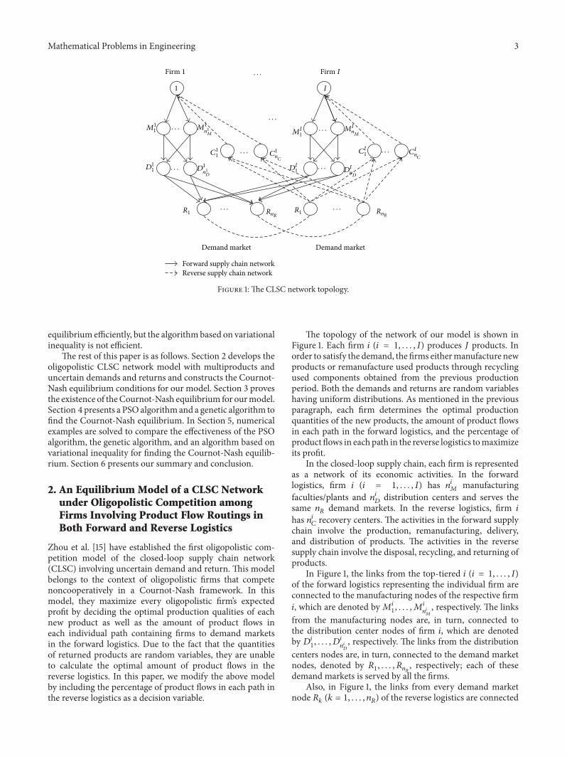
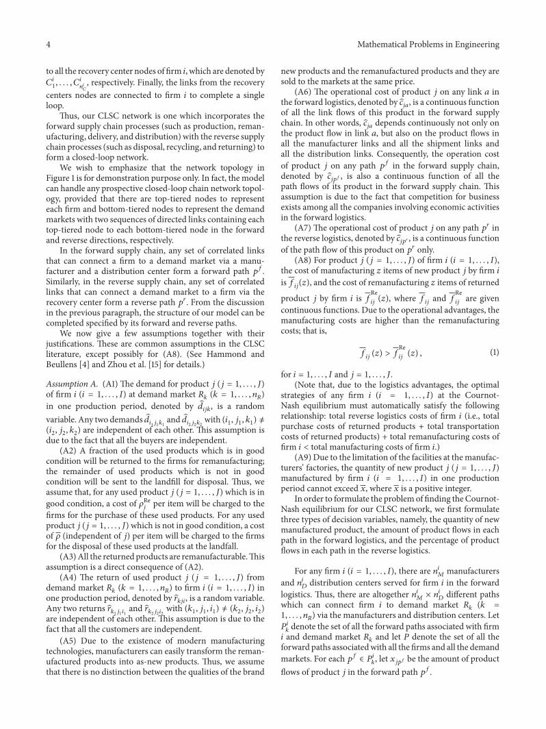
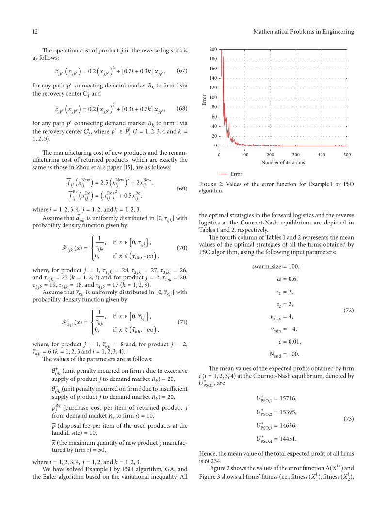
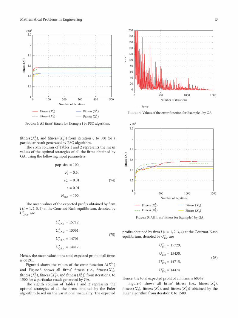
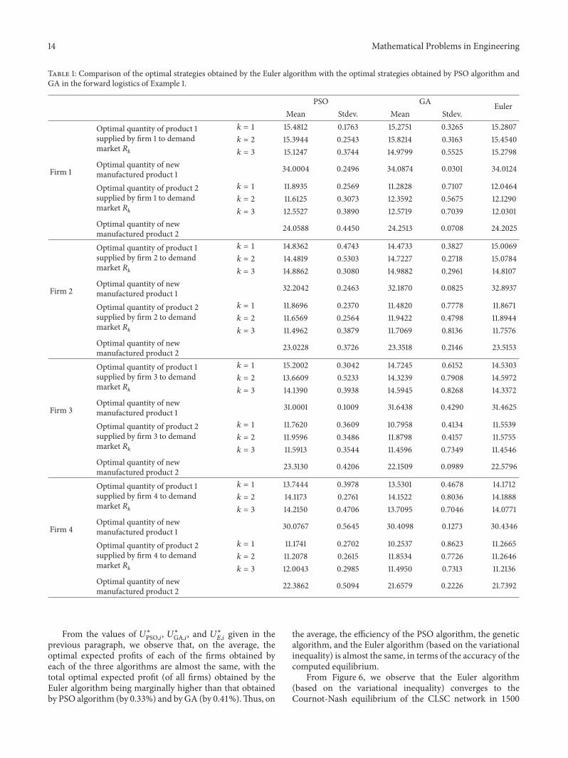
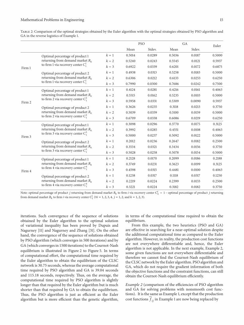
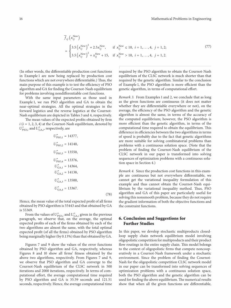
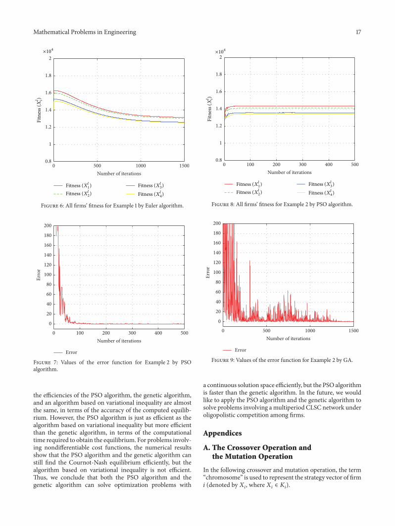
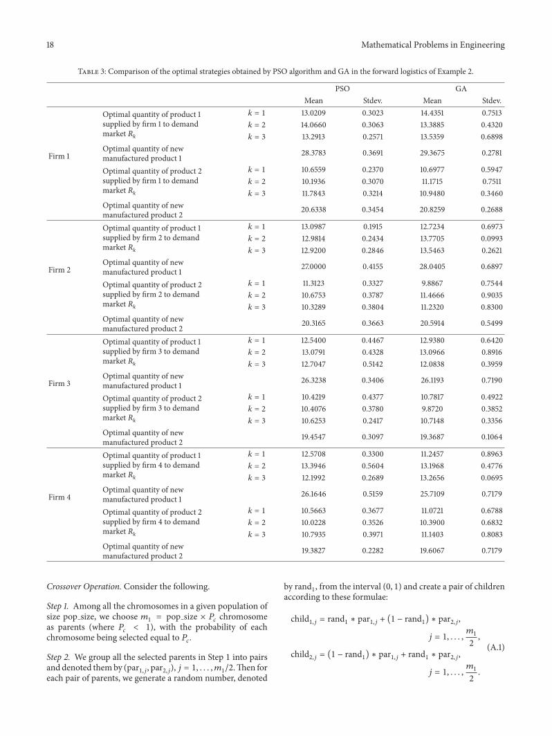
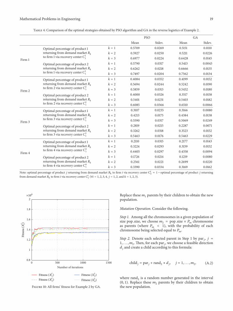
Recommended