\
https://ntrs.nasa.gov/search.jsp?R=19910004424 2018-05-20T21:00:24+00:00Z


NASAContractor Report 4338
AVSCOMTechnical Report 90-C-020
Non-Linear Dynamic Analysis
of Geared Systems
Rajendra Singh, Donald R. Houser,
and Ahmet Kahraman
Ohio State University
Columbus, Ohio
Prepared for
Propulsion Directorate
USAARTA-AVSCOM and
NASA Lewis Research Center
under Grant NAG3-773
National Aeronautics andSpace Administration
Office of Management
Scientific and TechnicalInformation Division
1990


NON-LINEAR DYNAMIC ANALYSES OF GEARED SYSTEMS
Rajendra Singh, Donald R. Houser, and Ahmet Kahraman
Ohio State University
Department of Mechanical Engineering
Columbus, Ohio 43210
Under the driving conditions, a typical geared system may be subjected to large
dynamic loads. Also, the vibration level of the geared system is directly related to the
noise radiated from the gear box. Accordingly, a good understanding of the steady
state dynamic behavior of the system is required in order to design reliable and quiet
transmissions. It is the main focus of this study with the scope limited to a system
containing a spur gear pair with backlash and periodically time-varying mesh stiffness,
and rolling element bearings with clearance type non-linearities. The internal static
transmission error excitation at the gear mesh, which is of importance from high
frequency noise and vibration control view point, is considered in the formulation in
sinusoidal or periodic form.
A dynamic finite element model of the linear time-invariant (LTI) system is
developed. Effects of several system parameters, such as torsional and transverse
flexibilities of the shafts and prime mover/load inertias, on free and forced vibration
characteristics are investigated. Several reduced order LTI models are developed and
validated by comparing their eigen solutions with the finite element model results.
Using the reduced order formulations, a three-degree of freedom dynamic model is
developed which includes non-linearities associated with radial clearances in the radial
rolling element bearings, backlash between a spur gear pair and periodically varying
gear meshing stiffness. As a limiting case, a single degree of freedom model of the
spur gear pair with backlash is considered and mathematical conditions for tooth
IIiii__ .limllll01tai
iii
PRECEDING PAGE BLANK NOT RLMED

separation and back collision are defined. Both digital simulation technique and
analytical methods such as method of harmonic balance and the method of multiple
scales have been used to develop the steady state frequency response characteristics for
various non-linear and/or time-varying cases. Difficulties associated with the
determination of the multiple solutions at a given frequency in the digital simulation
technique have been resolved. The proposed formulation has been validated by
comparing the predictions with the results of two benchmark experiments reported in
the literature. Several key system parameters such as mean load and damping ratio are
identified and their effects on the non-linear frequency response are evaluated
quantitatively. Other fundamental issues such as the dynamic coupling between non-
linear modes, dynamic interactions between component non-linearities and time-varying
mesh stiffness, and the existence of subharmonic and chaotic solutions including routes
to chaos have also been examined in depth.
ACKNOWLEDGEMENTS
We are very grateful for the Financial support provided throughout this Ph.D.
research by the NASA Lewis Research Center, Department of Mechanical Engineering
and the Graduate School of the Ohio State University. Appreciation is also extended to
J. J. Zakrajsek and F. B, Oswald for providing some experimental results used in
Appendix D.
iv

TABLE OF CONTENTS
Page
ACKNOWLEDGEMENTS ............................................................ iv
LIST OF SYMBOLS .................................................................. viii
CHAPTER
I INTRODUCTION ............................................................ 1
1.1 Problem Formulation ..................................................... 1
1.2 Objectives ................................................................. 4
1.3 Development of Linear Time-invariant Models ....................... 6
1.3.1 Literature Review ................................................. 6
1.3.2 Mathematical Model ............................................. 8
1.3.3 Gear Mesh Formulation ......................................... 10
1.3.4 Finite Element Formulation and Eigen-Value Problem ...... 14
1.3.5 Forced Vibration Response .................................... 15
1.4 Parametric Studies ........................................................ 16
1.5
1.4.1
1.4.2
1.4.3
1.4.4
Modes of Interest ................................................ 16
Effects of Bearing Compliances ............................... 24
Effects of Shaft Compliances .................................. 24
Effects of Load and Prime Mover Rotary Inertias ........... 26
Reduced Order Linear Time-invariant Models ........................ 29
1.5.1 Single Degree of Freedom Torsional Model of Gear Pair... 29
1.5.2 Three Degree of Freedom Model .............................. 30
1.5.3 Six Degree of Freedom Model ................................. 32
1.6 Conclusion ................................................................ 36
V
II NON-LINEAR I_YNAMIC ANALYSIS OF A SPUR!
GEAR PAIR ...[
.................................................i.iiii.....ii2.1.1 Excitation Types and Backlash .................................
2.1.2 Literature Review ................................................i
2.2 Problem Formulation .....................................................
2.2.1 Physic al Model ...................................................
2.2.2 Scope and Objectives ............................................
2.3 Digital Simulation .........................................................
2.4 Armlytical Sol Jtion .......................................................
2.5 Comparison q f Two Solution Methods ................................
2.6 Parametric St udies ........................................................
2.7 Experimental Validation ..................................................
2.8 Comparison of Excitations ..............................................
2.8.1 Internal versus Extemal Excitation ............................
2.8.2 Periodic or Combined Excitation ..............................
2.9 Conclusion ................................................................
37
37
37
38
41
41
45
46
52
63
66
76
83
83
84
93
III NON-LINEAR DYNAMIC ANALYSIS OF A GEARED
ROTOR BEARING SYSTEM WITH MULTIPLE
CLEARANCES .............................................................. 95
3.1 Introduction ............................................................... 95
3.2 Problem Formulation .................................................... 97
3.2.1 Scope ............................................................. 97
3.2.2 Physical Model and Assumptions ............................. 99
3.2.3 Equations of Motion ............................................ 100
.2.4 Modeling of Non-linearities 103
3.3 @orresponding Linear Model ............................................ 107
3.4 Two Degree of Freedom System Studies .............................. 110
3.4.1 Equations of Motion ............................................ 110
3.4.2 Solution .......................................................... 111
3.4.3 Validation of Non-linear Bearing Model ..................... 114
vi

3.5
3.4.4 Non-linear Model Interactions ................................. 114
3.4.5 Internal versus External Excitation ............................ 121
Three Degree of Freedom System Studies ............................. 123
3.5.1 Classification of Steady State Solutions ...................... 123
3.5.2 Routes to Chaos ................................................ 124
3.5.3 Parametric Studies ............................................... 133
3.6 Experimental Verification ............................................... 149
3.7 Conclusion ................................................................ 163
IV INTERACTIONS
STIFFNESS AND
4.1
4.2
4.3
BETWEEN TIME-VARYING MESH
CLEARANCE NON-LINEARITIES ....... 164
Introduction ............................................................... 164
Problem Formulation .................................................... 165
Mathemalical Model ...................................................... 167
4.3.1 Equations of Motion ............................................. 168
4.4 Gear Pair Studies ......................................................... 172
4.4.1 Linear Time-varying System ................................... 173
4.4.2 Non-linear Time-varying System .............................. 177
4.4.3 Non-linear Time-varying Mesh Damping ..................... 181
4.4.4 Periodic _(t) and kh([) ........................................ 181
4.5 Geared Rotor-Bearing System Studies ................................. 187
4.5.1 Sinusoidal _(i) and kh(t) ..................................... 187
4.5.2 Periodic _(t) and kh(i) ........................................ 189
4.6 Experimental Validation ................................................. 194
4.6.1 Spur Gear Pair Dynamics ...................................... 194
4.6.2 Geared Rotor-Bearing System ................................ 196
4.7 Concluding Remarks ..................................................... 201
V CONCLUSION ............................................................... 202
5.1 Summary .................................................................. 202
5.2 Future Research Areas ................................................................ 204
REFERENCES .......................................................................... 206
APPENDICES ........................................................................... 216
vii

LIST OF SYMBOLS
b
c, C
d
e
f
F
g,h
H
I
Jk,K
L
m, M
n
N, N*
P
q
t
T
U
U
v
w
X
Y
Y
Z
backlash
viscous damping coefficient
diameter
static transmission error
non-linear displacement function
force
non-linear functions
total number of rolling elements in contact
rotary inertia
imaginary number
stiffness
length
mass
power of non-linear bearing function
describing functions
relative displacement
displacement
time
torque
mass unbalance of the gear
relative displacement
gear ratio
displacement vector
coordinate axis at the direction pertmndicular to the line of action
coordinate axis at the direction parallel to the line of action
relative displactment
transverse displacement
number of rolling elements
angular position of the rolling element in contact
viii

E
¢_p
K
0
0
0.)
f_
dynamic compliance
Kronecker delta
geometric eccentricity of the gear
phase angle
an angle
dimensionless stiffness
rotational displac_'nent
stress
natural frequency
excitation frequency
damping ratio
mode shape
Subscripls:
a
b
C, cl
d
e
gl
g2
h
i
JL
m
n
P
P
R
r
S
ahemating component
bearing
reference quantities
dynamic
extemal
pinion
gear
gear mesh
internal
an index
load or left
mean component
natural
prime mover
period
rightmode index or response
stress
ix
sl
s2
S
t
T
X
Y
I, II, m
driving shaft
driven shaft
static or modal index
inner contact
torque
coordinate axis at the direction perpendicular to the line of action
coordinate axis at the direction paraUel to the line of action
modal index
Supercripts:
T matrix transpose
-- dimensional quantities t
- amplitude of a harmonic function
derivative with respect to time
^ stiffness or force ratio
t All dimensionless quantities are without any superscript.
x

CHAPTER I
INTRODUCTION
1.1. PROBLEM FORMULATION
Dynamic analysis of geared systems is an essential step in design due to two
reasons. First, under the driving conditions, a typical geared system is subject to
dynamic forces which can be large. Therefore, the prediction of dynamic loads,
motions or stresses is needed in developing reliable gear trains. Second, the vibration
level of the geared system is directly related to the noise radiated from the gear box. An
attempt in designing quiet gears requires a good understanding of the dynamic behavior
of the system and the gear mesh source. Accordingly, the main objective of this study
is to develop accurate mathematical models of a generic geared rotor-bearing system
shown in Figure 1 .la. Of interest here is to investigate several key modelling issues
which have not been addressed in the literature, such as system non-linearities and
time-varying mesh stiffness.
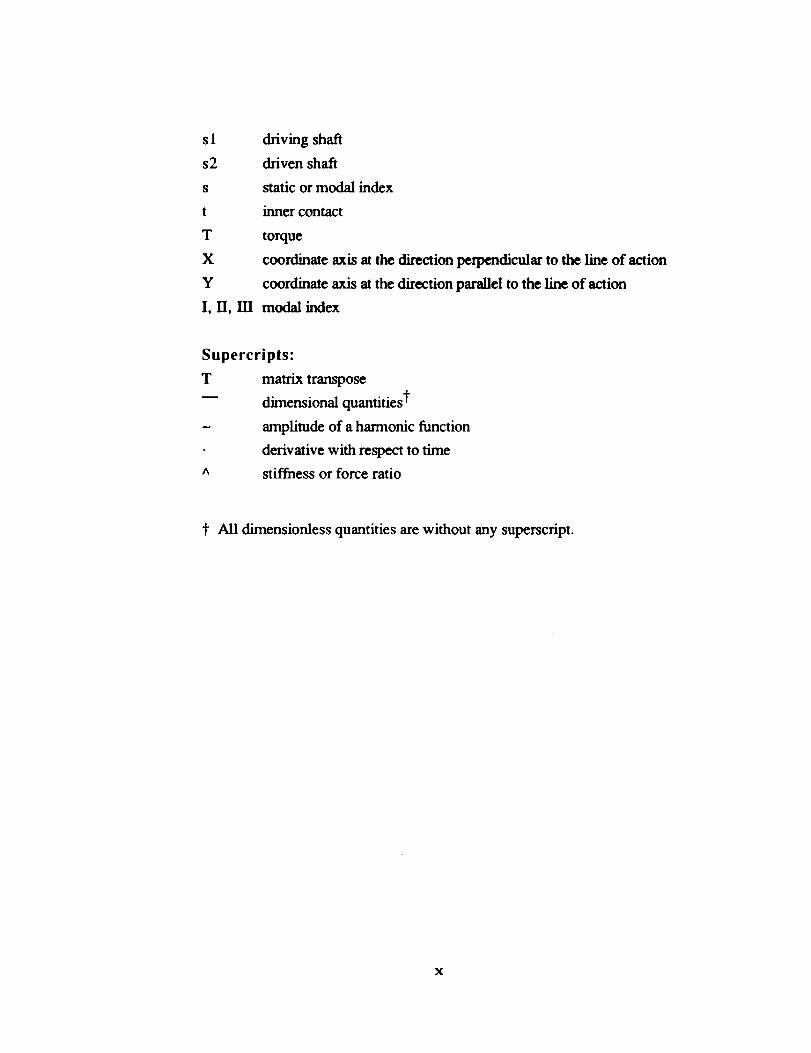
The generic geared system shown in Figure 1.1a consists of a single spur gear
mesh of ratio Vg=dg2/dgl, rolling element bearings, a prime mover driving the system
at Dsl speed and a typical inertial load. The system also includes other elements such
as couplings and flywheel. A discrete model of the system is shown in Figure 1. lb.
Here, shafts axe represented by discrete translational springs ks1 and ks2, translational
dampers Csl and Cs2, and torsional springs Ksl and Ks2. The gear mesh is represented
by a time-varying mesh stiffness kh([) and a non-linear displacement function fh
Rigid Gearbox
Prime Mover
-I
Flexible
CouplingGear
dg2,Ng2
dgl,NglRoilingElement
Bearings
_2
CInertialLoad
(a)
k_,cslY_
] Igl'mgl'dgl _b,C b
(Dikh,Ch
ke2,cs2,Ks2 kb'°o'
I g_,mg2,dg_
(b)
Figure I.I. a) A generic geared rotating system, b) discrete model of geared rotating
system.

which includes gear backlash. Further, linear time-invariant (LTI) mesh damping ch is
considered here. The roiling element bearings are defined by a time-invariant radial
stiffness k b subject to a non-linear displacement function fb, and an LTI damping
coefficient %. The prime mover and load are modeled as purely torsional elements of
inertias Ip and IL, respectively. The mean rotational speeds llsl and fls2 and the
geometric end conditions are such that gyroscopic effects are not seen.
The generalized displacement vector {r:l(t)}, associated with the inertia elements,
consists of angular displacements 0 and transverse displacements g and y. The
goveming equation of motion for the non-linear, time-varying multi-degree of freedom
model can be given in the general form as
[M]{_"(t )} + [C]{q' (t)} + [K(t)]{ f(q(t))} = {F(t)} (1.1)
where [M] is the time-invariant mass matrix and {_(i)} is the displacement vector.
Here, damping matrix [C] is assumed to be LTI type, as the effect of the tooth
separation and time-varying mesh properties on mesh damping are considered
negligible; validity of this assumption will be examined later. The stiffness matrix
[K(i)] is considered to be time-varying, given by a periodically time varying matrix
[K(i)] = [K(_ + 27r / _h)] where _h is the fundamental gear mesh frequency. The
non-linear displacement vector {f(_(_))} includes the radial clearances in bearings and
the gear backlash, and the forcing vector _'P(t)} consists of both external excitations
due to torque fluctuations, mass unbalances and geometric eccentricities, and an
intemal static transmission error excitation.
3

1.2. OBJECTIVES
Specific objectives of this study are given as follows; each chapter, written in the
journal paper style, deals with one major objective.
First, a dynamic f'mite element model of the linear time-invariant (LTI) system
given in Figure 1.1a is developed. Effects of several system parameters, such as
torsional and transverse flexibilities of the shafts and prime mover/load inenias, on free
and forced vibration characteristics are investigated. Three different reduced order LTI
models will be derived and the conditions under which these are valid will be
determined by comparing the eigen solutions with the finite element model results.
Development and verification of such a reduced order (with a very few degrees of
freedom) linear model is an essential step before the non-linear dynamic behavior is
analyzed [Chapter I].
Second, non-linear frequency response characteristics of a spur gear pair with
backlash are examined for both extemal and internal excitations. The internal excitation
is of importance from the high frequency noise and vibration control viewpoint and it
represents the overall kinematic or static transmission error. Such problems may be
significantly different from the rattle problems associated with external, low frequency
torque excitation. Two solution methods, namely the digital simulation technique and
the method of harmonic balance have been used to develop the steady state solutions
for the internal sinusoidal excitation. Difficulties associated with the determination of
the multiple solutions at a given frequency in the digital simulation technique have been
resolved as one must search the entire initial conditions map. Such solutions and the
transition frequencies for various impact situations are found by the method of
harmonic balance. Further, the principle of superposition can be employed to analyze
the periodic transmission error excitation and/or combined excitation problems
4

provided the excitation frequencies are sufficiendy apart from each other. Predictions
are compared with the limited experimental data available in the literature [Chapter l]].
Third, non-linear frequency response characteristics of a geared rotor-bearing
system are examined. A three degree of freedom dynamic model is developed which
includes non-linearities associated with radial clearances in the radial rolling element
bearings and backlash between a spur gear pair; time-invariant gear meshing stiffness is
assumed. The bearing non-linear stiffness function is approximated for convenience
sake by a simple model which is identical to that used for the gear mesh. This
approximate bearing model has been verified by comparing steady state frequency
spectra. The applicability of both analytical and numerical solution techniques to the
multi degree of freedom non-linear problem is investigated. Proposed theory is
validated by comparing the results with available experimental data. Several key
issues such as non-linear modal interactions and differences between internal static
transmission error excitation and extemal torque excitation are discussed. Additionally,
parametric studies are performed to understand the effect of system parameters such as
bearing stiffness to gear mesh stiffness ratio, altemating to mean force ratio and radial
bearing preload to mean force ratio on the non-linear dynamic behavior. A criterion
used to classify the steady state solutions is presented and the conditions for chaotic,
quasi-periodic and subharmonic steady state solutions are determined. Two typical
routes to chaos observed in this geared system are also identified [Chapter m].
Fourth, this study extends the non-linear single degree of freedom spur gear pair
model of Chapter II and multi-degree of freedom geared rotor-bearing system model of
Chapter nl by including time-varying mesh stiffness kh(i), and investigates the effect
of kh(i) on the frequency response of lightly and heavily loaded geared systems.
Interactions between mesh stiffness variation and system non-linearities associated with
5

gear backlash and radial clearances in rolling element beatings are also considered.
Resonances of the corresponding linear time-varying (LTV) system associated with the
parametric and external excitations are identified using the method of multiple scales.
Theoretical results are validated by available experimental results [Chapter IV].
1.3. DEVELOPMENT OF LINEAR TIME-INVARIANT MODELS
1.3.1. Literature Review
The study of geared rotor dynamics requires that the coupling between torsional
and transverse vibrations be included in the model. Although several modeling and
solution techniques such as lumped mass models and the use of the transfer matrix
method have been applied to rotor dynamic problems, the finite element method (FEM)
seems to be a highly efficient and accurate method for linear modeling. In one of the
early examples of FEM applied to a single rotor, Nelson and McVaugh [1] used a
Rayleigh beam finite element including the effects of translational and rotary inertia,
gyroscopic moments and axial load. Zorzi and Nelson [2] extended this by including
internal damping. Later, Nelson [3] developed a Timoshenko beam by adding shear
deformation to the Rayleigh beam theory. This model was further extended by
Ozguven and Ozkan [4] to include all possible effects such as transverse and rotary
inertia, gyroscopic moments, axial load, internal hysteretic and viscous damping and
shear deformations in a single model. However, none of the rotor dynamics models
described above can handle geared rotor systems, although they are capable of
determining the dynamic behavior of rotors which consist of shafts supported at several
points and carrying rigid disks at several locations.
Gear dynamics studies, on the other hand, have usually neglected the lateral
vibrations of the shafts and bearings, and have typically represented the system with a
6

linear torsional model. Although neglecting transverse vibrations might be a good
approximation for systems having stiff shafts, it has been observed experimentally [5]
that the dynamic coupling between the transverse and torsional vibrations due to the
gear mesh affects the system behavior considerably when the shafts are compliant.
This fact directed the attention of investigators to the inclusion of transverse vibrations
of the shafts and the bearings in mathematical models. Lund [6] developed influence
coefficients at each gear mesh for both torsional and lateral vibrations, obtained critical
speeds and a forced vibration response. Hamad and Seireg [7] studied the whirling of
geared rotor systems supported on hydrodynamic bearings; torsional vibrations were
not considered in this model and the shaft was assumed to be rigid. Iida, et al. [8]
considered the same problem by taking one of the shafts to be rigid and neglecting the
compliance of the gear mesh, and obtained a three degree of freedom model to
determine the first three vibration modes and the forced vibration response due to the
unbalance and the geometric eccentricity of one of the gears. Later, Iida, et al.
[9,10,11] applied their model to a larger system which consists of three shafts coupled
by two gear meshes. Hagiwara, Iida, and Kikuchi [12] developed a simple model that
included the transverse flexibilities of the shafts by using discrete stiffness values, and
studied the forced response of geared shafts due to unbalances and runout errors. They
included the damping and compliances of the journal bearings and assumed a constant
mesh stiffness. Although most of these gear dynamics studies have discussed several
aspects of the problem, none of them has been able to represent a geared rotor-bearing
system completely since almost all of them have used one or more simplifying
assumptions such as rigid shafts, rigid bearings, rigid gear mesh etc. which may not be
applicable to a real system. L_ addition, these studies proposed lower order lumped
mass linear models.
Neriya, et al. [13] employed a dynamic finite element model which eliminates
many of the simplifying assumptions. They found the forced vibration response
of the system at the shaft frequency, excited by mass unbalances and runout errors of
the gears by using the modal summation. But they did not consider the high
frequency, internal, static transmission error excitation which has the major role in
noise generation. An extensive survey of linear mathematical models used in gear
dynamics analyses is given in a recent paper by Ozguven and Houser [14].
1.3.2. Mathematical Model
Here, we assume linear bearings and no tooth separations with time-invariant
mesh stiffness, i.e. [K] ;e [K(t)] and {f(_(_))} = {q(_)}. Then the corresponding LTI
form of equation (1.1) is:
(1.2)
Since many investigators have modeled the generic system shown in Figure 1.1 a as a
single degree of freedom model, our analysis uses it as a reference model to transform
the governing equation into the dimensionless form. Focusing only on the gear pair as
shown in Figure 1.2, the equation of motion of the semi-defmite system is given in
terms of the relative translational displacement __(i)= (dgl0g 1 - dg20g2) / 2
d2ff([) d'6(t) -- F(i)mcl _ +Ch--'_+khU(t) = (1.3a)
where mcl is the equivalent gear pair mass defined as
8

Igl ,dgl
e(t) () ig 2 ,dg2
Figure 1.2. A single degree of freedom dynamic model.
9

fD n --
_4-_gl+ 4Ig2 :
(1.3b,c)
First, we establish the dimensionless time t as t = O_ni. Second, we use the base circle
diameter of the pinion dgl and the equivalent mass m c1 as characteristic length and
mass parameters, respectively, to obtain the governing equations in the dimensionless
form as
[M]{_(t)} + [C]{q(t)} + [K]{q(t)} = {Fm } + {Fah(t)} + {FaT(t)}" (1.4)
where an overdot means derivative with respect to time t, and the dimensionless forcing
vector consists of a mean force vector { F m } and two time-varying components: a) high
_equency excitation due to the kinematic gear transmission error { Fah(t ) } and, b) other
excitations due to mass unbalance Ugi, geometric eccentricities (run-out errors) Egi and
prime mover and load torque pulsations Tgia(t), typically at low frequencies, are
combined into a single term {FaT(t)}.
1.3.3. (;ear Mesh Formulalion
The gear mesh is represented by a pair of rigid disks connected by a translational,
viscously damped spring along the pressure line which is tangent to the base circles of
the gears as shown in Figure 1.3. By choosing the Y axis on the pressure line and the
X axis perpendicular to the pressure line, the transverse vibrations in the X direction
10

Ygl Pinion
II ._.___ _gl + dglOtl / 2 +_gl sin Ot1
)e(t)
' kh Ch
_g2 +dg2Ot2 / 2+Cg2 sinOt2/
Figure 1.3. Model of gear mesh used in FEM.
11

are uncoupled from both the torsional vibrations and transverse vibrations in the Y
n
direction. The dynamic mesh force Fhy at the mesh point in the Y direction can be
written in terms of the symbols given in Figure 1.3 from the rigid body dynamics
_ay(i) = Ch(Ygl + _0tl + £glflsl COS0tl -- Yg2 - _22 0t2
-Eg2_s2 COS0t2 - _Nglf_sl cos(Ngl0tl)) + kh(Ygl + _-_0tl
dg 2 a+Eg 1sin 0tl -Yg2 - T ut2 - Eg2 sin0t2 - el sin(Ngl0tl ))
(1.5)
Here, only the fundamental component of the static transmission error _(_) is
considered, i.e. _(i)= 8sin(Nglflsli ) where Ng 1 is the number of teeth of gear gl.
Dynamic mesh force FhY also introduces moments _hgl and _hg2 about
instantaneous centers of the gears:
Thgl (i) = F'hy (t)(_-_ + I_gl cos 0tl ) (1.6a)
Thg2(t) = -Fhy (i)(_'_ + £g2 cos 0t2) (1.6b)
The total angular rotation 0ti of the i-th gear is 0ti(t ) = _si _ + 0gi(t ) , i=1,2. The
displacement vector can be decomposed into two parts as {9} = {V:ls} + {V:lh} where
{V:ls}= [gl,yt,01,....,gj,yj,0j,....,Xn,yn,0n], j= 1ton, j_: gl, j:_ g2 (excluding the
degrees of freedom of the nodes where the gear and pinion are mounted) and
12

{_h} =[_gl,Ygl,0gl,_g2,Yg2,0g2], i=1,2. The coupling effect due to gear mesh is
only seen in the terms governed by {Fth} and the mesh stiffness [Kh], which
represents this dynamic coupling due to gear mesh is obtained from equations (1.5) and
(1.6) as
[Kh] - kh
0 0 0 0 0 0
0 1 dg---_-I 0 -1 dg2
2 2
0 dg---_-I d2---_l 0 dgl dgldg22 4 2 4
0 0 0 0 0 0
0 -1 dgl 0 1 dg22 2
0 dg2 dgldg2 0 dg2 d2----_22 4 2 4
(1.7a)
Since mesh viscous damping is proportional to the mesh stiffness,
In the overall force vector, non-zero terms correspond to displacements {qh } and are
given in the following form:
13

Ug l['121 sin Q'sl_ + F(t)l
Ugl_21 cosflslt
2Tglmcos _'_slt + _l(i) + Tgla(t)
dg I Egl
Vg2a2 sinas2i - _l(i)
Ug2L"I22 cos _'_s2i
2Tglm g2ahcOSas2i-d2--aF,(i)- %2a(il
dgl
(1.8a)
FI (i) - c h (Eg2f_s2 cos fls2i - I_glflsl cos flsli + _ Nglflsl cos(N glflsl i))
+kh(Eg2 sin _'_s2[ - £gl sin ['_sli + e sin(NglL'2sli)) (1.8b)
where Tglm is the mean input torque.
1.3.4. Finite Element Formulation and Eigen.Value Problem
The f'mite element method has been employed in obtaining stiffness and mass
matrices of the system of equations (1.4). The shafts are discretized and five degrees of
freedom are defined at each node, only the axial motion being excluded. The stiffness
and mass matrices of each f'mite rotor element are derived by using the variational
principle [3,4,15]. The system overall matrices are obtained by combining element
matrices, dynamic coupling matrices due to gear mesh defined by equation (1.7),
assumed bearing damping values and stiffnesses, and the inertias of the gears and other
lumped inertia elements. Here, [M] is diagonal and positive definite and [K] is
symmetric and positive semi-definite. The equation describing the undamped free
vibration of the system is obtained from equation (1.4) as
14
[M]{/_(t)} + [K]{q(t)} = {0}. (1,9)
The assumed form of the solution {q(t)} = {qa } cos(tot + 0) is substituted into equation
(1.9) to obtain the standard eigen-value problem:
[K]{qa} = to2 [M]{qa}. (1.10)
The solution of equation (1.10) yield the eigen-vectors or modes {Vr} and associated
eigen-values or natural frequencies oar. Here, a torsional rigid body mode at to=0
exists since [K] is semi-def'mite.
1.3.5. Forced Vibration Response
The excitation given by equation (1.8) (for no torque pulsations, i.e.
Tgla (t)= Tg2a ({) = 0) is the sum of three sinusoidal terms at frequencies flsl, fls2 and
gear mesh frequency Ngl_sl
2(1.11)
The steady state displacement response of the system due to this excitation is assumed
to be
2
{q(t)} = i_l [[_gi ]{Fgi } sin(_sit + _si) + [[_h ]{F_h} sin(Ngll:'_slt + _h) (1.12)
15
where [_gi] i=l, 2 and [_h] are the dynamic compliance matrices in the frequency
domain corresponding to the excitation frequencies, t2sl , f_s2 and Ngl_sl ,
respectively.
i = 1, 2; (l.13a)
n
I d=,z, Iv'"v'J -- 0_2- (Ngl[).si + 2j_rNglI),siCOr
(1.13b)
{_r} represents the r-th mass matrix-normalized modal vector, n is the total number of
degrees of freedom of the system, j = ,fL-_, and _r is the damping ratio for r-th mode.
See Appendix A for the computer code GRD which uses the theory given here.
1.4. PARAMETRIC STUDIES
1.4.1. Modes of Interest
The generic system shown in Figure 1.1 is modeled by FEM to examine the
natural modes of a general linear geared rotor-bearing system and to study the effects of
several system parameters on the dynamics of the system. Two numerical data sets as
listed in Table 1.1 are used. Predicted natural frequencies and modes for Set A are
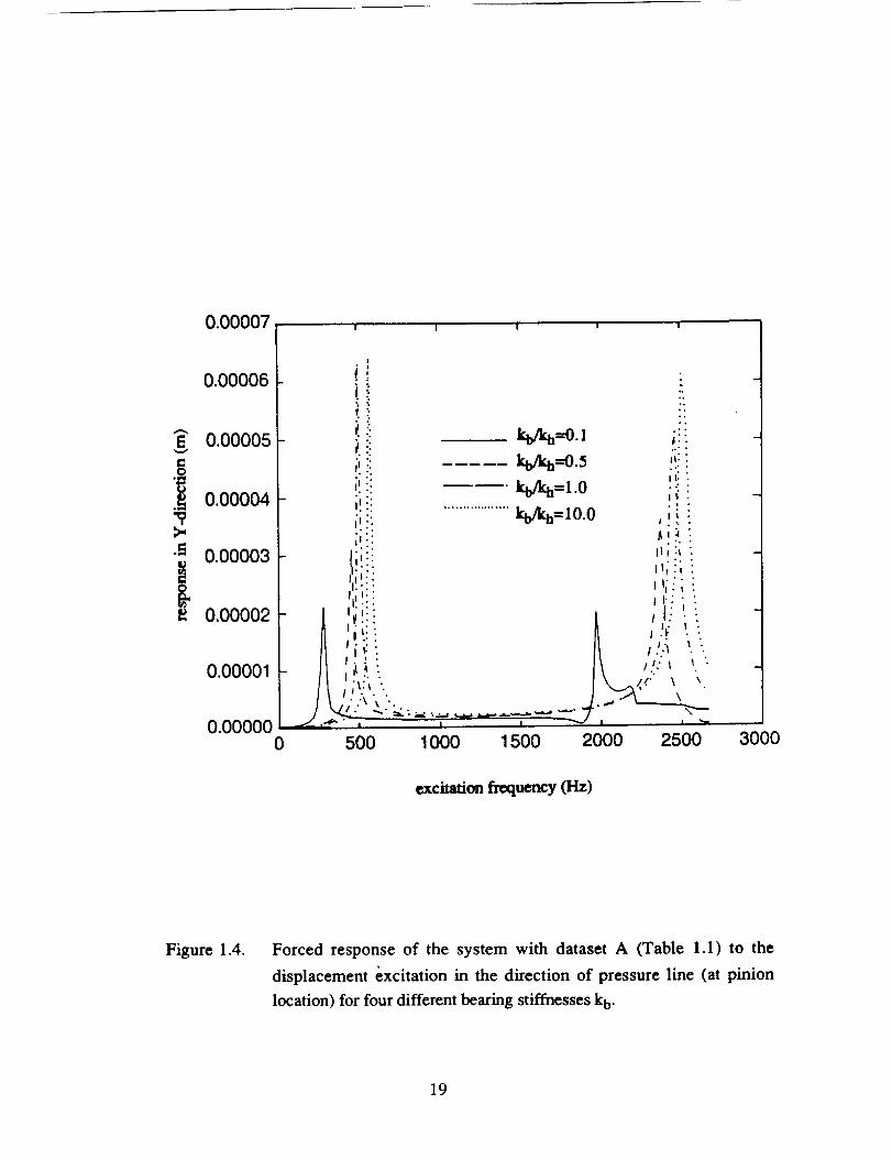
presented in Table 1.2. The response of the system to [(t) is also computed; Figures
1.4, 1.5 and 1.6 display the response in the Y and torsional directions at the pinion
location and the dynamic load to static load ratio at the mesh point dglF, hy /2Tmgl,
respectively. The system has no peak responses at the modes corresponding to motion
in the X direction since the excitation is applied in the Y (pressure line) direction, and
16

Table 1.1 Numerical data sets of the system used for calculations.
Parameters Set At Set B
Igl, Ig 2 (kg-m 2) 0.0018, 0.0018 0.0097, 0.0097
mgl, mg 2 (kg) 1.84, 1.84 3.45, 3.45
dgl, dg 2 (m) 0.089, 0.089 0.135, 0.135
Ng I 28 30
k h 1.0xl08 1.0xl08
k b (N/m) variable rigid
Lsl L, Lsl R (m) 0.127, 0.127 variable
Ls2L, Ls2 R (m) 0.127, 0.127 variable
KI, K 2 (N-m/rad) -- variable
Ip, IL (kg-m 2) -- variable
dsl,o, ds2,o (m) 0.037, 0.037 0.04, 0.04
dsl,i, ds2,i (m) 0., 0.01 --
(m) 9.3x10 -6 --
t NASA Lewis Research Center gear test rig.
17

Table 1.2. First 10 natural frequencies for set A of Table 1.1 (kb/kh=10).
Modal Modes of Natural Frequency tor Natural Mode
Index Interest Hz. Description
0 0
1 _I 581
2 687
3 _M 689
4 691
5 Vm 2524
6 3387
7 3387
8 3421
9 3421
torsional rigid body
first transverse-torsional coupled
X direction, transverse (driving shaft)
Y direction, transverse
X direction, transverse (driven shaft)
second transverse-torsional coupled
Y direction, transverse
X direction, transverse (driving shaft)
X direction, transverse (driven shaft)
Y direction, transverse
18
0.00007J I I I !
0.00006
0.00005
i 0.00004
"_ 0.00003
0.00002
0.00001
0000000
i
f
,!:!
;'ii
"t;"
)t-"
_:_""t:_
,:\ "_. "..
_" i I I
500 1000 1500
kly_---O.1
h,/_--o 5lq_kh=l.O
.................._,=io o
•.
It:
I t;
it:• =
I'tJ ..
fli :t
Ill!;
L 4"/" \,._l':i::f;i/.i.. i I ".
i1.." I ".
*..,,.-. \
2000 2500 3000
excitation frequency (Hz)
Figure 1.4. Forced response of the system with dataset A (Table 1.1) to the
displacement excitation in the direction of pressure line (at pinion
location) for four different bearing stiffnesses k b.
19
0.0035I I I I I
0.0030
0.0025
x 0.0020
0.0015
o 0.0010
0.0005
0.00000
!:
!t::
',[i:iq,/l_=O.l tt
!l.
k_/k_=O.S !;!tl
ioo/kb= 1.0 Ii
.............. 1oo/_..10.0 ';_ II .;
..t- I
I,t
- ' A ) ,
' // !t ,
m _: ,
_ ii t •tl" I "_
L A ,L,,: / _ ' ." ",| /I ,,i.i / L <::" .,/i_.__ ._- ..._. ___ s.-_ - \ /l '-"--q_. _ .... "-,_ I I _ I
500 1000 1500 2000 2500
excitation frequency (Hz)
t3000
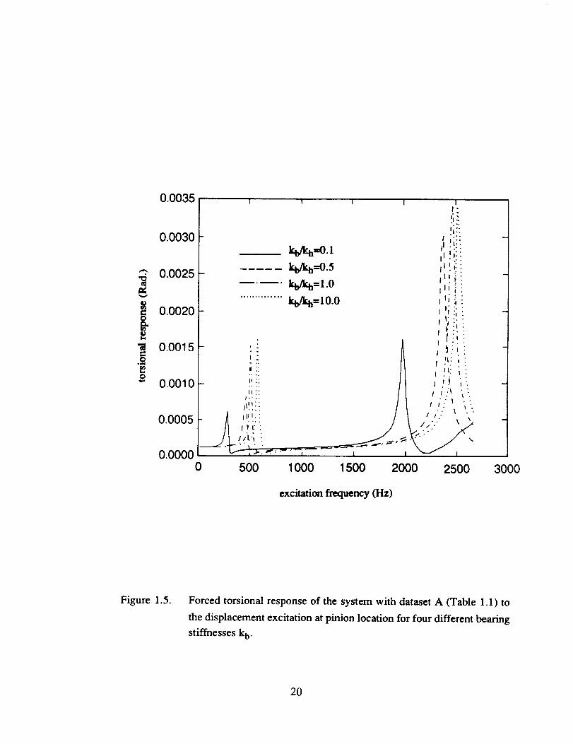
Figure 1.5. Forced torsional response of the system with dataset A (Table 1.1) to
the displacement excitation at pinion location for four different bearing
stiffnesses k b.
20

2.01 ! 1 I I
1.8
1.6
i1.4
1.2
.0 "/"A° |°* I
0 500 1000
_--'0.1
_=1.0
..................k_--_O.O!i:
t !ii
lJi;
l! :i
fi" -iU
]/ ,.'2***"', ",/\ /.:-" \..
1500 2000 2500
excitation frequer_ (Hz)
3000
Figure 1.6 Dynamic to static load ratio for dataset A (Table 1.1) due to the static
transmission error excitation for four different bearing stiffnesses k b.
21
the vibration in the X direction is dynamically uncoupled from the vibrations in the Y
and torsional motions, as described in the previous section. Therefore, the natural
modes corresponding to motions in the X direction can be eliminated when only _({)
excites the system. Accordingly, the following three typical modes are of special
importance:
I. First Transverse-Torsional Coupled Mocl) _I: This is the second mode listed
in Table 1.2 at 0.)I (581 Hz for the system considered). This mode corresponds to the
first peak in Figures 1.4 and 1.5 and its schematic shape is shown in Figure 1.7a.
Here, shafts move in opposite directions, gears vibrate in opposite directions also; but
transverse and torsional vibrations combine to yield small relative motion at the gear
mesh point. Therefore, dynamic loads at the mesh point are not large, resulting in no
peak in Figure 1.6 at _ while Figures 1.4 and 1.5 have peaks govemed by this mode.
II. Purely Transverse Mode _/II:- At this mode with natural frequency (Oil (689
Hz in Table 1.2), there is no torsional vibration and both shafts vibrate in phase in the
pressure line direction as shown in Figure 1.7b schematically. The relative
displacement at mesh point is zero since the gear ratio vg=l. Therefore, _(i) cannot
excite this mode as no peaks are observed in Figures 1.4, 1.5 and 1.6 at frequency (Oil.
IH. Second Transverse-Torsional Coupled Mode VIII_ The second and the
highest peak seen in Figures 1.4, 1.5 and 1.6 corresponds to this mode at 00ii I . As
seen from the mode shape illustrated in Figure 1.7c, both shafts and gears vibrate in
opposite directions, and transverse and torsional vibrations are additive at the mesh
point. Thus a large relative displacement at the mesh point is obtained, which results in
22

Z
a)first transverse-torsional coupled mode, _I
b) purely transverse mode, VII
c) second transverse-torsional coupled mode, • m
Figure 1.7. Typical natural modes of interest; see Table 1.2 for further details..
23

a large peak in Figures 1.4, 1.5 and 1.6. This is the mode at which the coupling
between transverse and torsional vibrations is very strong.
These three modes are observed in all geared rotor systems and they play an
important role in governing dynamic response of the system excited by _(_).
Therefore, any accurate mathematical model of the geared rotor-bearing systems must
be able to predict these modes.
1.4.2. Effect of Bearing Compliances
In most cases, radial stiffness of a typical rolling element bearings kb is roughly
of the same order of magnitude as the gear mesh stiffness kh; in general it lies in the
range 0.1kh<kb<100k h. Therefore, bearing flexibility should be included in the
analysis. A parametric study for data set A of Table 1.1 has been conducted to
demonstrate the effect of kb on the natural frequencies and the frequency response of
the system excited by E(t). Figures 1.4, 1.5 and 1.6 show the response in the Y and
torsional directions and the dynamic mesh load respectively for kb values ranging from
0.1k h to 10kh, shaft stiffnesses are being kept the same. An increase in bearing
stiffness results in an increase in both natural frequencies and the peak amplitudes.
Above the range of k b, the bearing becomes very rigid when compared to the shaft
compliances and its effect on the system can be ignored.
1.4.3. Effect of Shaft Compliance
Data set B of Table 1.1 has been used to study the effect of shaft compliance on
the natural modes. The shaft length is varied and the corresponding c.or values are
predicted by FEM; Figure 1.8 displays this resuh. The first natural frequency _ does
not change considerably with varying shaft length, whereas _ and _1I are strongly
24

g.
8
6
4
2
I
FEM
3-DOF model
, ! * A * !
u.O 0.2 0.4 0.6 0.8
shaft length/pinion diameter
Figure 1.8. Effect of the shaft length on the typical natural frequencies.
25

dependent on the shaft length, especially at smaller lengths. Another observation from
Figure 1.8 is that ¢Oli and ¢thiI become very large for smaller shaft lengths and clearly
move beyond the range of the operational speed of most geared rotor systems. In this
case, the first coupled transverse-torsional mode _I can be assumed to be uncoupled
from these two modes.
1.4.4. Effect of Load and Prime Mover Rotary Inertias
As shown in Figure 1.1, the shafts are connected to a prime mover and a load at
either end through flexible torsional couplings. The following parameters need to be
considered: motor and load rotary inertias, torsional compliances of the flexible
couplings, and stiffnesses of the driving and driven shafts.
First, the motor and load are assumed to be connected to the shafts without
considering any torsional couplings in between. Figure 1.9 displays the variation in
¢oI, ¢ol/and o)iII with a variation in the prime mover inertia. Here, data set B of Table
1.1 with Lsi=0.04 m is used. COl/and _ are not affected and therefore, the inertias of
motor and load can be disregarded if the major concern is to predict these two modes.
However, o3I is strongly dependent on prime mover and load inertias.
Second, the load and prime mover inertias are fixed (Ip=5Igl) and the torsional
springs K 1 and K2, which represent flexible couplings and shafts are varied. Figure
1.10 shows the variation in ¢or with changing K 1 and K 2. Here COil and ¢o[iI are again
not affected, as expected. On the other hand, o_ is almost constant (which is nearly
equal to the value yielded by zero prime mover and load inertias) up to a point and, it
starts increasing with increasing K. This indicates that the motor and load are isolated
from the geared rotor system when the in-between torsional elements are compliant
26

.o
4
2
III
FEM
...................... 6-1_F model
* I , I * , I * I ,
0 1 2 3 4 5
prime mover inertia/pinion inertia
Figure 1.9. Effect of the prime mover inertia on the natural frequencies.
27

8qo
o_
O
+
3.5
2.5
1.5
m
/..... ..... .°.._.....°. .......... .._......_.... .... .......°.°..°......
11
..... , o , • o , o I o .....
10' 10' 10'
torsional stiffness (N.m/rad)
Figure 1.10. Effect of the torsional stiffness K of the transmission elements in
between the gear box and the prime mover & load inertias on the natural
frequencies.
28

enough, which is the case in most practical systems. Under these circumstances,
motor and load inertias can be neglected in the analysis.
1.5. REDUCED ORDER LINEAR TIME-INVARIANT MODELS
In this section, three different reduced order analytical models of the geared rotor-
bearing systems shown in Figure 1.1 will be developed and the conditions and system
parameters at which these simple models can predict the dynamics of the system
accurately, will be discussed. The finite element model of Section 1.3 will be
employed as a reference model to check the validity.
1.5.1. Single Degree of Freedom Torsional Model of Gear Pair
As the simplest model, a single degree of freedom (SDOF) model of geared rotor
systems shown in Figure 1.2 is considered. The shaft and bearing flexibilities and the
motor and load inerfias axe not considered in this model. This model can only preclict a
single mode at a frequency o0n as defined in equation (1.3c) which corresponds to the
first transverse-torsional mode at ¢oI . Here, ¢Ol-Oe0n when shaft lengths Lsi-,0 and
bearings are very stiff. And, _ and e0ii I axe sufficiently beyond the operational speed
range and the variation in coI is assumed to be negligible with shaft length as shown in
Figure 1.8. Therefore, in some cases, the SDOF model of Figure 1.2 can be used to
represent the system provided these conditions axe met. For instance, for data set B of
Table 1.1 with Lsi=5 cm, a SDOF model can be utilized up to an operational rotational
speed of 6000 rpm which corresponds to the excitation frequency at 3000 Hz for
Ngl=30 teeth. As it is seen in Figure 1.8, only the first mode is observed and its
variation is not significant within 0._£1<3000 Hz and 0<Lsi._5 cm.
29
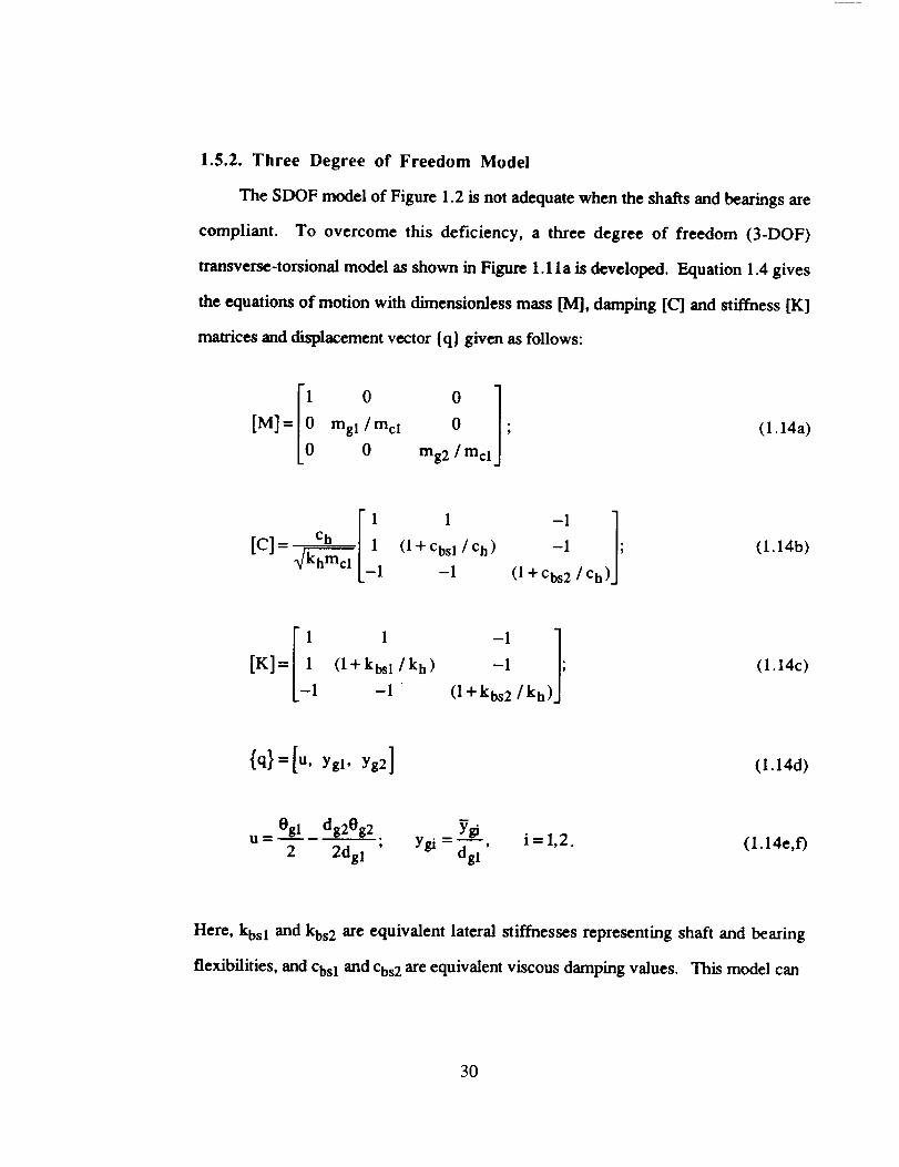
1.5,2. Three Degree of Freedom Model
The SDOF model of Figure 1.2 is not adequate when the shafts and bearings are
compliant. To overcome this deficiency, a three degree of freedom (3-DOF)
transverse-torsional model as shown in Figure 1.11 a is developed. Equation 1.4 gives
the equations of motion with dimensionless mass [M], damping [C] and stiffness [K]
matrices and displacement vector {q} given as follows:
0 0][M] = mg I / mcl 0 ;
0 mg 2 /mcl
(I.14a)
[!iCh (I+ CbsI/ch)
[C]= _ 1 -I -Il-I
(I+ Cbs2 /Ch)
(1.14b)
1 1 -1 ][K]= I (l+kbs Ilk h) -I ;
-1 -1 (l+kbs 2/k h)
(1.14c)
{q}=[u, Ygl, Yg2] (1.14d)
Ogl dg2Og2 Ygi, - -- i - 1,2. (1.14e,f)
u= 2 2dg 1 Ygi-dg 1,
Here, kbs I and kbs 2 are equivalent lateral stiffnesses representing shaft and bearing
flexibilities, and Cbs1 and Cbs2 are equivalent viscous damping values. This model can
30

Pinion
Igl ,m 0 ,dgl
Shaft & Bearing
r_l,Cb_ c h Gear Mesh
Excitation_
GeAr
Ig2, mg2,dg2 Shaft & Bearing
kbs2,Cbs2
(a)
Prime Mover
Ip_ Pinion
L_IL
Ns2, %s2
(b)
Figure 1.11. Reduced order analytical models of Figure 1.1; a) three degree of
freedom model, b) six degree of freedom model.
31

accurately predict all three modes of interest as evident from Figure 2.8 and Table 1.3
where its predictions are compared with the results of FEM.
When the system is connected to the motor and load inertias, then the in between
torsional stiffnesses K 1 and K 2 should be compliant enough to be able to neglect the
effects of the motor and load inertia.s, as it is discussed earlier in Section 1.4.4. In
summary, the 3-DOF model shown in Figure 1.1 la can be used to describe the
dynamics of the geared rotor system when: a) the shafts and bearings are compliant and
provided the shafts are short such that higher order bending modes of the shafts are out
of the frequency range considered, and b) the torsional stiffnesses of the connections in
between the motor and load inertias and the gear box are sufficiently compliant.
1.5.3. Six Degree of Freedom Model
A six degree of freedom (6-DOF) model as shown in Figure l.llb can be
employed to represent the geared rotor-bearing system when the effects of the motor
and load are not negligible as mentioned in Section 1.4.4. Equations of motion are still
given by equation (1.4) and the dimensionless system matrices are defined as
[M]=_ Imcl
-Ip/d21 0 0 0 0 0
0 I$1/d21 0 0 0 0
0 0 Ig2 / d251 0 0 0
0 0 0 IL/d21 0 0
0 0 0 0 msi 0
0 0 0 0 0 mg 2
; (1.15a)
32

Table 1.3. Comparison of typical modes obtained by FEM and 3-DOF models for set
B of Table 1.1; Lsi/dgl--0.3.
Mode V
VI VII VIa
Displacement FEM/3-DOF FEM/3-DOF FEM/3-DOF
0g 1 -0.012/-0.011 -0.001/0.0 -0.210/-0.246
0g 2 0.012/0.011 -0.001/0.0 0.210/0. 246
Ygl 1.0/1.0 1.0/1.0 - 1.0/- 1.0
Yg2 -1.0/- 1.0 1.0/1.0 1.0/1.0
33

1
[cl=
Cl CI 0 0
dg I 4 4
-symmetric -
(d _+ hVs c_a_=gl 4 ) - d_l
C2
d]t
0 0
c_.k _ c_k
2 2
2 2
0 0
(ch + CbsI ) --Ch
(ch + Cbs2
(1.15b)
1
K1 Kl+k__.)d_l 4
0 0
khVg0
4
(_-_--22 + khvg K 2-)K2
dgl
0 0
k__h_h _ k_.h_h2 2
_khV8 khV.___£g
2 2
0 0
-symmetric - (k h + kbs 1) -k h
(k h + kbs 2)
(I.15c)
{q} =[Op, Ogl, Og 2, 0 L, Ygl, Yg2 ] (1.15d)
For data set B of Table 1.1 predictions yielded by the 6-DOF model are compared
with those by FEM as shown in Figure 2.9 and Table 1.4. Based on these results, it
can be concluded that the 6-DOF model is accurate enough to predict the natural modes
of the system. Accordingly, 6-DOF model must be employed when the effects of the
motor and load are not negligible.
34

Table 1.4. Comparison of typical modes obtained by FEM and 6-DOF models for set
B of Table 1.1; Lsi/dgl=0.3, IFAgl=5.
Mode W
Displacement FEM/6-DOF FEM/6-DOF FEM/6-DOF
ep 0.079/0.079 0.002/0.0
eg I -1.0/-1.0 -0.005/0.0
eg 2 1.0/1.0 -0.005/0.0
0 L -0.079/-0.079 -0.002/0.0
Ygl 0.006/0.006 1.0/1.0
Yg2 -0.006/-0.006 1.0/1.0
-0.018t-0.013
1.011.0
-1.0t-l.0
0.018¢0.013
0.391 ¢0.451
-0.391 t-0.451
35

1.6. CONCLUSION
In this chapter, a finite clement model to investigate the dynamic behavior of
linear time-invariant geared rotor systems has been developed. The transverse
vibration of the system associated with shaft and bearing flcxibilitics and the dynamic
coupling between the transverse and torsional vibrations due to gear mesh have been
considered. Natural modes of the system have been identified and forced vibration
response due to both low frequency external and high frequency internal excitations
have been determined. Reduced order analytical models of the geared rotor bearing
system have also been developed. Three different linear timc-invariant models (SIX)F,
3-DOF and 6-DOF) have been suggested to represent the geared system. By
comparing results with FEM predictions, it has been shown that such reduced order
linear models are reasonably accurate. Therefore these models will be extended in
Chapters II, III and IV in analyzing the effects of system non-linearities and time-
varying mesh stiffness.
36

CHAPTER II
NON-LINEAR DYNAMIC ANALYSIS
A SPUR GEAR PAIR
OF
2.1. INTRODUCTION
2.1.1. Excitation Types and Backlash
The focus of this chapter is on the backlash non-linearity as excited primarily by
the transmission error between the spur gear pair. A gear pair is bound to have some
backlash which may be designed to provide adequate lubrication and eliminate
interference due to manufacturing errors. Backlash-induced torsional vibrations may
cause tooth separation and impacts in unloaded or lightly loaded geared drives. Such
impacts result in intense vibration and noise problems and large dynamic loads,
which may affect reliability and life of the gear drive [16,17]. Excitation mechanisms
can be grouped as follows:
A. External Excitations: This group includes excitations due to rotating mass
unbalances, geometric eccentricities, and prime mover and/or load torque fluctuations
[18]. Although mass unbalances and geometric eccentricities can be reduced through
improved design and manufacturing, torque fluctuations are not easy to eliminate
since they are determined by the characteristics of the prime mover (piston engines,
dc motors etc.) and load [19]. Such excitations are typicaUy at low frequencies _T
which are the first few multiples of the input shaft speed ['1s . Practical examples
include rattle problems in lightIy loaded automotive transmissions and machine tools
[19,20].
37

B. Internal _x_itatiQr_; This group includes high frequency _h excitations
caused by the manufacturing related profile and spacing errors, and the elastic
deformation of teeth, shafts and bearings. Under the static conditions, all such
mechanisms can be combined to yield an overall kinematic error function known as
"the static wanmfissi_-i error" _({-) [17,18]. This error is defined as the difference
between the actual angular position of the driven gear and where it would be ff the
gears were perfectly conjugate [17,18,21-23]. In gear dynamic models, _(t-) is
modeled as a periodic displacement excitation at the mesh point along the line of
action [15,24-26] and its period is given by the fundamental meshing frequency
_h =N_2s where N is the number of teeth on the pinion. Practical examples
include steady state noise and vibration problems in automotive, aerospace,
industrial, marine and appliance geared systems.
2.1.2. Literature Review
Experimental studies on the dynamic behavior of a spur gear pair with backlash
started almost 30 years ago and still continue [27-29]. As one of the better examples
of such experiments, Munro [27] developed a lightly damped (damping ratio 4=0.02)
four-square test rig to measure the dynamic transmission error of a spur gear pair.
He used high precision gears with rigid shafts and bearings, and showed
experimentally that the tooth separation takes place when the mean load is less than
the design load. Dynamic transmission error versus speed curves were plotted to
illustrate the steady state response and the jump phenomenon. Kubo [28] measured
the dynamic tooth stresses using a similar set-up in order to calculate the dynamic
38

factors. He also observed a jump in the frequency response of the gear pair with
backlash even though the test set-up was heavily damped (_0.1).
Such experimental studies, though limited in scope, have clearly shown that the
gear pair dynamics can not be predicted with a linear model - see Ozguven and
Houser [14] for a detailed review of the linear gear dynamic models as available in the
literature. Although most of the non-linear mathematical models used to describe the
dynamic behavior of a gear pair are somewhat similar to each other, they differ in
terms of the excitation mechanisms considered and the solution technique used. For
instance, a large number of studies have focused on the rattle problem in lightly
loaded geared drives which are excited by the low frequency external torque
excitations [30-35]. A few investigators have included the static transmission error
excitation in the non-linear models [24,35-37].
The gear backlash non-linearity is essentially a discontinuous and non-
differentiable function and it represents a strong non-linear interaction in the
governing differential equation. This issue has been discussed by Comparin and
Singh [33] and they have concluded that most of the solution techniques available in
the literature can not be directly applied to examine this problem. Most of the gear
dynamic researchers recognized this problem implicitly, and therefore employed
either digital or analog simulation techniques [19,24,29,35-38], For instance,
Umezawa et.al [29], Yang and Lin [32] and Ozguven and Houser [24] have solved a
one degree of freedom torsional model of the gear pair using numerical techniques.
Lin et.al. [38] included motor and load inertias in a three degree of freedom torsional
model. Kucukay [35] has developed an eight degrees of freedom model to include
the rocking and axial motions of the rigid shafts. In most of these studies, with the
exception of Umezawa's analysis [29] which did not include any backlash, a
39

discontinuity hasbeenseenin the frequencyresponsecharacteristics. But many
investigators have typically joined two discrete points to show a broad jump in the
frequency response curve [24,35,38]. Some of these problems have been due to the
numerical simulation techniques which may not work or may result in misleading
answers ff not employed properly. Such difficulties have been found by Comparin
and Singh [33], Singh et al. [34] and Gear [39-40] but are yet to be resolved or
addressed by the gear dynamics researchers. Accordingly, one of the major
objectives of this chapter is to examine whether numerical simulation techniques can,
in fact, be used to predict the dynamic response completely, and what precautions one
must take to develop such a mathematical model. Since Comparin and Singh [33]
and Singh et al. [34] have examined the external excitation problem, in this chapter
we focus mainly on the internal excitation and see whether the numerical simulation
technique can be made to work for the prediction of the non-linear frequency
response characteristics.
A few researchers have attempted to obtain the analytical solutions for a gear
pair problem, based on the piece-wise linear techniques which divided the non-linear
regime into several linear regimes [41-43]. For instance, Wang [41,42] has used two
and three degree of freedom torsional models with backlash, and assumed that the
gear teeth are rigid and the driven gear has an infinite inertia. The governing
equations have been solved using the piece-wise linear technique. It should be noted
that the piece-wise linear technique gives only solutions for the equivalent linear
systems and one typically may have difficulties in combining such solutions [43].
Comparin and Singh [33] overcame these problems by employing the harmonic
balance method (HBM) and constructed analytical solutions for the non-linear
frequency response characteristics of a gear pair with backlash as excited by the
4O

external torque. In this chapter, we will use the same technique to examine the
internal excitation problem, and compare results with digital simulation and
experimental studies. Further literature review is included in subsequent sections.
2.2. PROBLEM FORMULATION
2.2.1. Physical Model
A two degree of freedom semi-def'mite model of the spur gear pair with rotary
inertias Ig I and Ig 2 and base circle diameters dg I and dg 2 as shown in Figure 2.1 is
considered here. The shafts and bearings are assumed to be rigid. The gear mesh is
described by backlash of 2b and by a time _variant mesh stiffness k h ;e kh(i )
when in contact and viscous damping ch. The equations of torsional motion of the
gear pair as shown in Figure 2.1 are
d20gl dglC h (dgl d0gl dg2 d0g2 d_ /Igl_+ 2 2 dt 2 d]" dr"
dt
dgl (_ dg2 _ E(t'-)] = TgI(_" )+ "-'_"- _ 0gl-- --'_ 0g 2(2.1a)
d2092 dg2Ch (dgl dOgl dg2 dog2 d_)g2 ._2 2 2 d_" 2 d_ dt
dt
-"T" mOg---T-eg2- (2.1b)
41

pinion
Igl, dg_ "_0 gl
excitation _'(_(
0
b
)
g_ gearg2' dg2
Figure 2.1. Gear pair model.
42

- 2(/.) = I" + I"g2a (/.) are torqueswhere _'gl(t) = I"glm + l"gla (/.) and Tg g2m
on pinion and gear and f is a non-analytical function essentially describing the mesh
elastic force as shown in Figure 2.1. Here, output torque fluctuation Tg 2a(/.) will
be neglected to simplify the dynamic problem, i.e. T g2(/.) = 1"g2m" Equations
(2.1a) and (2.1b) can be reduced to one equation in terms of Tt(/.) which is defined
as the difference between the dynamic transmission error g(/.) and the static
transmission error [(/.).
d2_
mcl _ + Ch _ + khf(q(/))= Fm + FaT(i) - mc d-_ ;Ot Ot
(2.2a)
dg I 1(i- ) dg 2_(t-) --g(i-) - _'(O = -T" 0g 2 0 g2(t--) -- E'(_) ; (2.2b)
+4I
gl
mc2 = dg I(2.2c,d)
Fm 2Tglm 2Tg2m . l_aT(_" ) =- d = d '
gl g2
2mcTgla(t-)
m c2dgl
; (2.2e,f)
T(_(t-)) {_(tO -b;f(_(i')) = kh .= 0;_(i') + b;
r_(tO> b
-b< r_(i') <b
_(i') < - b
(2.2g)
43

where mcl is the equivalent gear pair mass, Fm is the average force transmitted
through the gear pair, FaT(t') is the fluctuating force related to the external input
torque excitation and f(_(/-)) is the nonlinear displacement function. Equation
(2.2a) is nondimensionalized by letting q(/') =_(i') / b, _n = _/kh/mcl ,
t = _nt" and _ = c h / (2mclean). Now, consider harmonic excitation for both
e(t') and FaT(t-) as e(t-)- 2"sin($D-ht +0h), PaT(t-)--_ aTSin(_"_T _- +0T)
where _2 h and _'_T are the fundamental excitation frequencies of internal
displacement and external torque fluctuations, respectively. Further, define
dimensionless excitation frequencies fl h = _-1h / Con a n d fl T-- _ T / _ n,
dimensionless external mean load F m = _ m / bk h' amplitudes of the dimensionless
internal (Fi(t)) and external alternating forces (Fe(t)) FaT-l_aT/bkh and
F a_ = _"/b and nonlinear displacement function f(q(t)) to yield the following
governing equation of motion.
q(t) + 2_cl(t) + f(q(t)) = P(t) (2.3a)
F(t)- Fro+ FaTsin(_Tt +0 T) +Fahf12h sin(flht +O h ) (2.3b)
q(t)- 1; q(t) > 1f(_(t)) 0; - 1 < q(t) < 1
f(q(t)) - b - (2.3c)q(t) + 1; q(t) <- 1
44
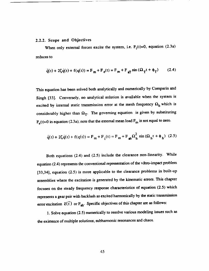
2.2.2. Scope and Objectives
When only external forces excite the system,i.e. Fi(t)=0, equation (2.3a)
reducesto
_(t)+ 2_c_(t) + f(q(t)) - Fm+ Fe(t)- Fm+ FaT sin (f_Tt + _T ) (2.4)
This equation has been solved both analytically and numerically by Comparin and
Singh [33]. Conversely, no analytical solution is available when the system is
excited by internal static transmission error at the mesh frequency fl h which is
considerably higher than fiT" The governing equation is given by substituting
Fe(t)-_ in equation (2.3a); note that the external mean load Fm is not equal to zero.
2 sin(_h t+#h ) (2.5)di(t) 4- 2_Cl(t) ÷ f(q(t)) = F m ÷ Fi(t) = F m 4. Fahfl h
Both equations (2.4) and (2.5) include the clearance non-linearity. While
equation (2.4) represents the conventional representation of the vibro-impact problem
[33,34], equation (2.5) is more applicable to the clearance problems in built-up
assemblies where the excitation is generated by the kinematic errors. This chapter
focuses on the steady frequency response characteristics of equation (2.5) which
represents a gear pair with backlash as excited harmonically by the static transmission
error excitation _(/-) or Fall. Specific objectives of this chapter are as follows:
1. Solve equation (2.5) numerically to resolve various modeling issues such as
the existence of multiple solutions, subharmonic resonances and chaos.
45

2. Construct analytical solutions to equation (2.5) using the harmonic balance
method (HBM) which has been applied successfully to solve equation (2.4) by
Comparin and Singh [33].
3. Compare digita/simulation and harmonic balance techniques and establish
the premises under which the jump phenomenon can be predicted.
4. Perform parametric studies in order to understand the effects of F m, Fah and^
on the frequency response. Vary the force ratio F =Fm/Fah which is a measure of
the load on the gear pair and compare the dynamic behavior for lightly and heavily
loaded gears.
5. Validate analytical and numerical solution techniques by comparing these
with previous experimental studies [27,28].
6. Compare the frequency response characteristics of equations (2.4) and (2.5),
and also examine the possibility of finding overall response when both extemal and
internal excitations are applied simultaneously.
7. Consider the periodic static transmission
k
F(t)= F m + Fi(t)= F m + _ (jflh)2 Fahjj=l
three (k=-3) harmonics axe included.
error excitation case, i.e.
sin (jflht + _bhj) ; only the first
2.3. DIGITAL SIMULATION
Clearance or vibro-impact problems in single degree of freedom systems have
been examined by a number of investigators whose formulations are similar to
equation (4) - see Comparin and Singh [33] for a detailed review. Moreover, Shaw
and Holmes [43] and Moon and Shaw [44] have considered an elastic beam with one
sided amplitude constraint subject to a periodic displacement excitation, and have
46

shownexperimentally and numerically that the chaotic and subharmonic resonance
regimes exist. Whiston [45-47] has investigated the non-linear response of a
mechanical oscillator preloaded against a stop. He has solved the system equation for
harmonic excitation by digital simulation and studied the existence and stability of the
subharmonic and chaotic responses and the effect of preload on chaos. Similarly,
Ueda [48] has solved the Duffing's equation, _ + 2_Cl + q3 = F sin t, numerically
and defined the regions of different solutions on a _ versus F map. According to
him, the existence of harmonic, subharmonic and chaotic responses depends on
values of 4 and F, and multiple steady state solutions typically exist. Thompson and
Stewart [49] have reviewed the available literature, with focus on the Duffing's
equation. It should be noted that equation (2.5) is different from the non-linear
differential equations considered by the above mentioned studies. Therefore,
equation (2.5) must be studied in depth as the results of the other non-linear equations
may not be directly applicable to our case.
First, we solve the governing non-linear differential equation (2.5) numerically
using a 5th-6th order, variable step Runge-Kutta numerical integration routine
(DVERK of IMSL [50]) which is suitable for a strongly non-linear equation
[33,39,40]. Second, we investigate the existence of chaos and subharmonic
resonances. Since the steady state response of the system due to the sinusoidal
excitation is of major interest, it is necessary to run the numerical program for a
sufficient length of time. The number of cycles of the forcing function required to
reach the steady state depends on 4.A
A lightly loaded system (F=Fm/Fah=0.5) with low damping (4--0.02) is
considered as the first example case. For Fm=0.1 and Fah=0.2, the response q(t) is
computed over the frequency range 0 < fl h < 1.5. Figure 2.2 shows phase plane
47

plots el(t) vs. q(t) for different _h values. For £_h=0.3, all transients converge to
one periodic solution at the fundamental frequency £_h of the forcing function
irrespective of the initial conditions q(0) and el(0) • Therefore, it is called a "period-
one, tp " attractor where tp=2g/i"l h. But, in the case of flh---O.5, three coexisting
period-one attractors have been found as shown in Figure 2.2. Here, q(0) and Cl(0)
define three steady state limit cycle solutions. For all initial conditions given by
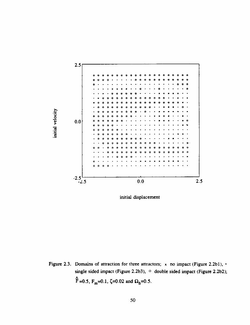
- 2 < q(0 ) < 2 and - 2 < Cl(0 ) < 2, a map of the domains of attraction for each
steady state solution is obtained in the map in Figure 2.3. If a smaller increment is
used for the initial conditions, a f'mer resolution will be obtained. Hence each phase
plane plot shown in Figure 2.2 is strictly governed by a subset of the initial
conditions. Similarly, two period-one attractors are found at flh=0.6. At flh=0.7 ,
besides two period-one tp attractors, two more solutions of period 3tp exist, i.e.
period-three attractors. But only a period-two 2tp attractor is seen when flh=0.8.
Within the range 1. 0 < £_ h _ 1. 5, non-periodic, steady state or chaotic response is
observed. Figure 2.4 shows the chaotic time history and the Poincare map (strange
attractor) at D.h=l.0. These results are qualitatively, but not quantitatively, similar to
the studies reported on the Duffing's equation [48,49] and clearance non-linearity
(equation (2.4) type) [33].
It is concluded that the subharmonic response of period ntp provided n ;_ 1 and
the chaotic response (tp _ .o) are seen in the gear pair only for a certain set of
^parameters Fro, F, _ and fl h. It must also be noted that the multi-solution regions
are strongly dependent on the choice of q(0) and el(0). Only one steady state
solution can be found via digital simulation when only one set of initial conditions is
chosen at a given fZh, and the rest of the steady state solutions are not predicted. This
48

0.01
(a) (hi)0.04
-0 IN , , ,
q 1.12 1.O q
1.0
-I.0-2.0
1.0
-0.5
(b3) (cX)0.5
q
-1.0
1.2 q 2.(
(c2)
-2.0
2.(]
-2.0-0.5
q 2.0 0 q 1.6 -2.0 q 3.0
(dl) (d2) (d3)
0.5l
q 2.0 0.2 q 1.6 -0.5 q 2.q
-2,
2.(
,i
(d4) (c) (O
0.51
-3.o
ql
-0.51
q 3.0 0 q 1.4 -2.0 q 2.0
Figure 2.2.A
Phase plane plots of steady state solution q(t) for F =0.5, Fm=O.l, _=0.02
and for different t'),h values; a) _h"-0.3, b) _h--0.5, c) fib=0.6, d) _h=0.7,
e) flh=0.8, f)flh=1.0.
49
¢J
2.5
0.0
000000000000000000000
0000.*...000000000000
0.,-*-.,,*'***,**''000
Iteellll eOe OelleeO
aOOOOOOOOOOOOOO* I.n
MOOOOOOOOOOOOOOOOOOm*
*OOOOOOOOOOOO**umm,O*
OOOOOOOOO*O WUmlN*m
OOOOOOOOO**,*mums* u*
OOOOOOO.***.**uu_. mO
*********************
*********************
OOOOOOO*,,****,*oMU"
OOOOOOOOOO***,,mn *,
OOOOOOOOOOOO*-*.**O*
00-000000000000000000
OOOOOOOOOOOOOOOOOO
I OOOO*,**,,**,,*m
O**.*****.lN_muwmmx*.
*********************
-2.5 ' '-_'.5 0.0 2.5
initial displacement
Figure 2.3. Domains of attraction for three attractors; x no impact (Figure 2.2bl), •
single sided impact (Figure 2.2b3), o double sided impact (Figure 2.2b2);
^
F=0.5, Fm---O.l, 4=0.02 and t_h=0.5.
50

(a)
2.0
q
-2.05O
I t t I i t t t t
t / tp 75 100
2.0
q
-2,0100
t/ tp 125 150
0.5
0
-0.5
.°A(m
Co)
i
L 4.."..a rt'__ !_
-1.0-2.0 - ll.O 0
q
|
1.0 2.0
Figure 2.4. Chaotic response of a gear paff;
time history, b) Poincare map.
A
F=0.5, Fro=0.1 , ¢=0.02 and _h=l.O; a)
51

results in an incomplete frequency response description. These issues will be
discussed further in Section 2.5.
^A heavily loaded system with F =2, Fm=0.1 and the same amount of damping
4=0.02 is considered as the second example case. Figure 2.5 shows the phase plane
plots for the same values of fl h which are used in the first example case. Unlike the
f'u'st example case, no chaotic responses are found here. All of the solutions are
period-one tp type for all flh<l.0 and Figure 2.6 shows the typical domains of
attraction at f_h=0.6. However, within the range 1. 0 < fl h < 1. 5, one period-two
A
attractor co-exists with the period-one orbit. Hence the force ratio F determines the
existence of the chaotic and subharmonic responses. To illustrate this point, consider
A
chaos shown in Figure 2.4. As F and _ are increased, significant changes in the
response are observed in Figures 2.7 and 2.8. A transition from the chaos to a
period-two, and then to a period-one steady state solution is seen when _ is
increased from 0.75 to 1.0 and then to 1.5. Similarly, an increase in _ to 0.05
reduces chaos to a period-eight attractor, which then bifurcates to a period-two orbit
at _--0.1 as shown in Figure 2.8. Since most real geared systems are heavily loaded
^with a high F, chaotic and subharmonic responses should not be seen under the
normal driving conditions. This issue will be discussed again in section 2.6.
2.4. ANALYTICAL SOLUTION
An approximate solution for equation (2.5) is constructed using the harmonic
balance method (HBM). Assume that q(t) = qm + qa sin(flht + #r) where qm and qa
are mean and alternating components of the steady state response, and # r is the
phase angle. Here, higher harmonics of the response are not included in the analysis.
52

0.002
(a)
q 1.105
(b)
0.01
-0.01 , , .1.08 q 1.12
0.4
q
-0.4
(cl)
L2 q 1.6
0.02
-0.02
(c2) (dl)
0.04
1.07 q 1.13
q
-0.04.
0.4
q
-0.4
(d2)
1.05 q 1. L _.4 q 1.4
0.1
4
(el) (e2) (fl)
1.2
0.4:
q q 1.4
0.4
q
1.3q
(r_)
-1.0
-0.5 q 2.{
Figure 2.5.A
Phase plane plots of steady state solution q(t) for F =2, Fm=0.1, 4=0.02 and
for different D h values; a) flh=0.3, b) _h--0.5, c) f_h=0.6, d) _h=0.7, e)
_h---0.8, f) _h-l.O.
53

u
2.5
0.0
-2.5 .....-2.5 0.0 2.5
initial displacement
Figure 2.6. Domains of attraction for two attractors; x no impact (Figure 2.5c2), • single^
sided impact (Figure 2.5cl); F--2, Fm=0.1, 4=0.02 and flh-0.6.
54

(a)
4.0
-2.0
2.0
q
o5o
t / tp 25 - ..__t. 50
tIt. 75 ] _ 100SteadyState
_o)
......... I
I I I I I I I I I
t/tp 7,3 50
:2.0 .........
q
0
(c)
40. .........
-2.0 .... 2.5 .... 5 }t / t p _ Steady State
Figure 2.7. Time histories of q(t) for Fah=0.2,A
c)F=I.5.
A A
_=0.02 and a) F=0.75, b)F=l,
55

(a)2.0, v T i i I "r _ T
q
-I.0
t/tp 50
Co)2.0 .........
-1.0 , , , , , , , ,
t/tp 25 50
2tp
A
Figure 2.8. Thne histories ofq(t) for Fm--O.1, F--0.5 and a) 4--0.05, b) 4=0.1.
56

The quasilinear approximation to the nonlinear function f(q) with the excitation
2F(t) = F m + Fi(t) = F m + Fahfl h sin (fl ht + ¢ph ) is in the form [33,51]
f(q) =Nmqm + Naqa sin (f'_ ht +Or) + Naqa COS(flht +(_r) (2.6)
where the describing functions N m, N a and N_ are defined as:
2_
Nm _ 1 Sf(qm + qa sin _0)dtp ; (2.7a)2_:qm 0
2_
1 Sf(qm +qa sin (p)sin q)cl_o ; (2.7b)Na- /l:qa o
2_
Na*- gqal o'If(qm+q'sin _0)cosq_dtp; tp=flht+0 r . (2.7c,d)
Equation (2.3b) is substituted into equations (2.7a), (2.7b) and (2.7c) to obtain
Nm= 1qa 1
2qm[g(y+)-g(Y-)] ; Na= 1- _[h(_'+)+h()'-)] ;(2.Sa,b)
1 + qm (2.8c,d)N_ = 0 ; _/+ - qa
where
57

g(y) = "/+ - ;
I(2.8e)
°1 (sm-1 ;y<-I •
y>l
(2.8f)
Comparin and Singh [33] used tnmcated series expansions for functions g(y) and
h(y) given by equations (2.8e) and (2.80. They stated that the error involved in
using truncated series is within 6 percent when only the frost two terms are considered
with the coefficient of the second term adjusted to yield the actual value for y = 1.
Using the same approach, one gets
g(Y)---2(I+(-_)Y2); h(Y)---_'_-'(Y-('-_)Y3); ,_S1 (2.9a,b)
and obtains the following frequency response by substituting equations (2.6) into
equation (2.5) and equating the coefficients of like harmonics:
2Fah_ h
qa=_( 2 ;N a-a2h) +(2_ah) 2
e m
)qm = Nm (2.10a,b)
( 2_12h )Or = O h - tan- 1 .... 2 (2.10c)
Na- _h
58

Depending on the damping ratio _ and the parameters F m, Fall and f_ which
define the excitation, there are three cases at which different solutions are obtained:
(a) no impact (no tooth separation), (b) single sided impacts (tooth separation, but no
back collision), and (c) two sided impacts (back collision).
Case I: No Impact : The tooth separation (impact) is not observed in a geared
system if the displacement q(t) lies in the region q(t)>l all the time. This condition,
shown in Figure 2.9 as case I, can be described mathematicaJly as
Iqm +qal >1 and Iqm-qal >1 (2.11)
Then, for no impact region in which the conditions defined by equation (2.11) are
satisfied, the describing functions are given by
N m= l- _qm " Na = I • (2.12a,b)
Substitution of equations (2.12) into equations (2.9) yields the following governing
equations for no impact case
2Fahfl h
qal = _/(1 _ _,./2h) 2 + (2_f/h)2 ;
qmI =Fro+ 1 ; (2.13a,b)
.( 2_n,. )-Chi=0p tan- . (2.13c)l-K1
59

/ __2q../!double sided 2q-m| /I i
impact (Ill) _ | ' / _ I-1 / I _ , ,
/ I f I
/qm.m 1 qmnqmI q
no impact(z)
single sidedimpact 0I)
Figure °2.9. 111us_rationof different impact regimes.
6O

Hence, when there is no tooth separation, the system is linear and the mean and
ahemating components of the response, qm and qa, are uncoupled from each other.
The transition frequencies from the no impact (linear) regime to the other non-linear
regimes where tooth separation occurs are found by substituting q a = [q m - 11 into
the equations (2.13a) and (2.13c) as
= + ...... -tFmJ J
1 Fa h 2
(2.14)
where _"_tl and i')t2 are the transition frequencies from no impact to single sided
impact regimes below and above resonance, respectively.
Case II: Single Sided Impact : Mathematically, the single sided impacts (tooth
separation without back collision) are observed if
qm +qa > 1 and qm- qal < 1 • (2.15)
As illustrated in Figure 2.9 as case 11, the solution remains in the region q(t) > - 1.
The describing functions satisfying equation (2.15) are in the form
qau 1 [1 + h(y_)] (2.16a,b)Nm= 1- 2qmi I [y+-g(y_)] ; Na= 1- _"
61

Substitution of equations (2.10a) and (2.10b) into equations (2.16a) and (2.16b)
gives the describing functions for the single sided impact case:
qaII f2F /_-2_ 21 1
Nm= 1+ 2qml1- _'_'[1 +_,'-_--_-),'t'-)J- (y+)j ""(2.17a)
Na = 21 _ 2(1- qm11) [1 _ (__)(__)1"_-q'_ (2.17b)
Then equations (2.9a), (2.9b) and (2.9c) with the describing functions given by
equations (2.17a) and (2.17b) define the response of the system in the single sided
impact region. In this case, it is hard to find closed form expressions for transition
frequencies from single sided to double sided impact regions. The validity of the
solutions, obtained by solving equations (2.9) and (2.17) iteratively, should he
checked. If the solution does not satisfy equation (2.15), then single sided impacts
are not seen at that particular frequency.
Case HI: Double Sided Impact : The double sided impact case exists ff qm and
qa are such that the following conditions are satisfied:
qa>ll-qml and qa>ll+qml (2.18)
Figure 2.9 (case IU) shows the double sided impact case at which qa is large enough
when compared to qm so that back collision is observed. The describing functions
62

for thiscaseareobtainedfrom equations(2.8a)and(2.8b)under the condition given
by equations (2.19):
2(re - 2)
7rqam
qmm (2.19a,b)3
qa_
The solution for the double sided impact case is obtained by solving equations
(2.9) and (2.19) numerically. The validity of the solution, again, should be examined
by using the conditions defined by equation (2.18), as it is done in the single sided
impact case.
The solutions of all three regimes are combined to obtain the overall frequency
response of the gear pair. Figure 2.10 illustrates typical qa versus fl h and qm versus
t2 h plots. All three impact regimes are shown on these plots. Also we note the
frequency region where multiple steady state solutions are obtained.
2.5. COMPARISON OF TWO SOLUTION METHODS
First, we validate the approximate analytical solutions of equation (2.5) by
comparing predictions with the results obtained by digital simulation. Again, two
example cases (a heavily loaded system and a lightly loaded system) are considered
and the frequency response curves qa versus flh and qm versus fl h are generated.
^Figure 2.11 shows the frequency response for the heavily loaded system with F =2,
Fro=0.1 and 4--0.05. Numerical and analytical results agree very well as both predict
amplitudes and the transition frequencies for case I (no impact) and case II (single
sided impact) regimes, and both show that the double sided impact solutions do not
exist. These results demonstrate that the analytical solutions are indeed correct for the
63

2
0_.0
(a)
'0
°loo
oo o case I
A ca..sell
o casein
T
Jrr_nnr _nno°°°°°O° - , , /
0.5 1.0 1.5
frequency
2
0u.{
n
A
O
(b)
caseI
caseH
case HI
[_OOr_O000[] O000000DO00
T Tm , • i , i i a ! i ,
0.5 i .0 1.5
frequency
Figure 2.10. Typical frequency response plots for a gear pair; a) qa versus f2h,b) qm
versus f_h"
64

heavily loaded system. Now consider the lightly loaded system as the second^
example case with F=0.5, Fm=0.1 and 4=0.05. From Figure 2.12 we note that
while case I and case II solutions as yielded by both solution techniques are very
close to each other, case Ill regime is predicted only by the analytical expressions.
Why is case lXl not predicted by the digital simulation7 To answer this consider the
following:
a) In digital simulation, several sets of q(0) and /l(0) must be tried to find all
of the steady state solutions within a multi-valued region, for instance
0.6 "_ fl h _ 0.7 in Figure 2.11 and 0.4 _ fl h < 0.7 in Figure 2.12. When q(0)
and /l(0) are kept constant for each D,h or ff the steady state solution of the previous
frequency is used as the basis for the initial conditions for the next frequency
considered, only one of the solutions can be found while missing the other(s).
Figure 2.13 illustrates this point as the steady state solution of the previous frequency
is used here for the initial conditions at each fl b. Using this procedure, case U
solutions within the multi-valued regions are missed. Therefore, whenever digital
simulation is used to solve the equation of motion, dependence of the steady state
solutions on q(O) and el(0) must be taken into account to avoid the risk of obtaining
an incomplete frequency response description.
b) In the case of Figure 2.12, no initial conditions governed by case III are
found by the digital simulation within the range of initial conditions - 2 < q(0 ) < 2
and -2 < el(0)< 2 we have considered. Conversely, the analytical method
predicts this regime as the issue of initial conditions is irrelevant here. To illustrate
65

A
this, first we consider the case of Figure 2.3 with F=0.5, Fro=0.1 , 4=0.02 and
flh--0.5. Figure 2.14a shows the domain of attraction governed by case III within
the range - 2 < q(0)< 2 and - 2 < tt(0)< 2 with a q(0) or tt(0) increment of
0.2. Here, almost half of the initial conditions considered define case Ill solutions.
Therefore the chance of having a double sided impact solution at flh=0.5 is
considerably high. Now, increase the damping to _--0.03. Once again a case 11I
regime is predicted analytically, but the number of initial conditions corresponding to
case IN is not sufficiently high like the case of 4--0.02. In the digital simulation, the
transient solution will converge to case I or case II solution unless the initial condition
corresponds to one of those shown in Figure 2.14b for case IZI. And the limiting
case is reached when _=0.04, while holding the other parameters the same; now no
initial conditions corresponding to case lIl are found. Obviously there might be
initial conditions, out of the range considered, which correspond to the analytical
results. Therefore the existence of case III solutions should be checked numerically
by searching the entire range of initial conditions as defined by the physical
considerations of the system.
2.6. PARAMETRIC STUDIES
Frequency response amplitudes, transition frequencies and the existence of
various impact regimes depend on F m, _ and 4. Therefore, a set of parametric
studies using analytical solutions of section 2.4 will be presented here; same results
can be duplicated by the digital simulation technique. First we examine the effect of^
Fm and F while holding the damping ratio _ equal to 0.05. Figures 2.15 and 2.16
^compare results for four different F values obtained by varying Fah for a given
^
Fro=0.1. Both gears maintain complete contact with each other when F is very
66

0.50
0.25
(a)
theory
o digital simulation
_equency
1.5
1.25
1.00
(b)
0.75 ......
u.O 1.0 1.5
theory
u digital simulation
i i i a !
0.5
_equency
Figure 2.11. A
Comparison of theory with numerical simulation; Fro=0.1 ' F =2, _=0.05;
a)qa versus f_h, b) qm versus f2 h.
67

2.5
2.0
1.5
1.0
0.5
"-- theory
° digital simulation
(a)
/
u.O 0.5!
1.0 1.5
frequency
2
0V.(
(b)
theory
D digital simulation
i !
0.5
frequency
I i
1.0 1.5
Figure 2.12. A
Comparison of theory with numerical simulation; Fm=O. 1, F =0.5, _=0.05;
a) Cla versus _h, b) qm versus i'_h.
68

0.50
(a)
0.25
---- theory
= digital simulation
D
o%_ °frequency
.5
Figure 2.13.
(b)
2.5
2.(
1.5
1.(]
---- theory
digital simulation
/
0.5 "''_---- --- -: -----= :-,_
o__ _frequency
Comparison of theory with numerical simulation when initial conditions are^ ^
kept constant; Fm=0"l' _=0.05; a) F =2, b) F =0.5.
69
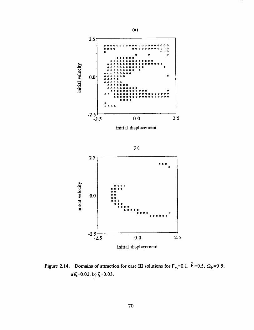
¢.)
C>
0
2.5
0.0
(a)
000000000000000000000
0000 000000000000
0 000
0 0
000000
00000000000000
000000000000000000
000000000000
000000000 0
000000000
0000000
00000
000000
0000000
0000000000
000000000000 0
O0 000000000000000000
000000000000000000
0000
o
o000
-2.5-2.5 0.0 2.5
initial displacement
"d
2._"
0.0
(b)
000
0000
0000
O0
oo
O0
000
000
0o00
o0000
0000
000000
-2.5-2.5 0.0 2.5
initial displacement
Figure 2.14.A
Domains of attraction for case HI solutions for Fro=0.1, F =0.5, f_h=0.5;
a)_=O.02, b) _=0.03.
70

A
large, say F=10 in Figures 2.15a and 2.16a. Consequently the dynamic system is
linear and the mean qm and altemating qa components of the torsional motion are
^uncoupled as expected. However, for F =2, no-impact regime (case I) can not cover
the whole frequency range and a region around the resonant frequency is dictated by
the single sided impacts (case II). Away from the resonance, over the range given by
D,h>0.8 and D,n<0.7, solutions are single-valued, whether case I or case II solutions.
Conversely, near the resonance given by 0.7<f/,h<0.8 dual-valued solutions are seen
in Figures 2.15b and 2.16b. And sudden discontinuities are observed, i.e. a jumpA
up at 12h=0.g and a jump down at _2h=0.7. When F is reduced further, double
sided impact (case ILI) solutions start to appear in Figures 2.15c and 2.16c. Now, the
frequency range of interest can be divided into the following four regions: i) case I,
f_h<0.4; ii) case I and case III, 0.4<_h<0.6; iii) all three cases, 0.6<f2h<0.625; and
A
iv) only case II, 1)h>0.625. Region (ii) disappears at F >0.5.
ANext, we vary F by changing F m for a given Fah =0.05. This set of
parameters does not yield any double sided impacts (Case m). Again, the tooth pair
A A
does not lose contact when F is large enough, say F210 and only the linear
A A
solutions exist as shown in Figure 2.17a. But when F is lowered to F=4, 2 and I,
the response is non-linear which is composed of cases I and II as shown in Figures
2.17b-d.
Next we examine the role of damping ratio _ on the frequency response in Figure
2.18, given Fro=0.1 and Fah=2. Double-sided impacts are found at a low damping
value 4=0.025 as shown in Figure 2.18a. When _ is increased to 0.05, case III
solutions no longer exist and case I and case II solutions define the frequency
response completely. The jump-up and jump-down transition frequencies in Figure
2. lgb are distinctly apart. With an increase in _, transition frequencies approach each
71

0.12
0.06
(a)
0.5 1.0 1.5
frequency
0.4
U
(b)
/
0.5 1.0 1.5
frequency
2
i
U.0
(c) (d)
//
j I
..... J " " 0 _° ' • " ' '
0.5 1.0 1.5 u.( 0.5 1.0 1.5
_equency _uency
Figure 2.15.Frequency response qa for different alternating loads; Fro=0.1 , _=0.05,A A "A A
a)F=10, b) F=2, c) F=l, d) F=0.5.
72

(a)
N
0"_.0 0.5 1.0
frequency
1.5
1.0
(b)
f
i i - ' • - i ....
1.5 0"0.0' 0.5 1.0 1.5
frequency
1.5
1.0
_0.5
(c) (d)1.5
• . _ J .... I " " 0 0" • * I • • • L •O'0v.0' 0.5 1.0 1.5 0. • 0.5 1.0
frequency frequency
.5
Figure 2.16. Frequency response qm for different alternating loads; Fro=0. I, _=0.05, a)A A A A
F=10, b) F=2, c) F=I, d) F=0.5.
73

0.6(a)
0.5 1.0 1.5
frequency
0.6
(b)
0.5 1.0 1.5
frequency
0.6
42
(c)
0.5 1.0
frequency
0.6
"_ 0.3
(d)
.5 0._. 0,n 0.5 1.0 1.5
frequency
Figure 2.17. Frequency response qa for different mean loads; Fah=0.05, _=0.05, a)A A A A
F=IO, b) F-.--_, c) F=2, d) F-I.
74

4
0u.0
(a)
/0.5 1.0 1.5
frequency
0.4
(b)
J0.0 ' _ .......
u.O 0.5 1.0 1.5
frequency
0.4
(c)
0.5 1.0
frequency
0.4
o
•_ 0.2
.5 °'°.o
(d)
0.5 1.0
frequency
.5
Figure 2.18.A
Frequency response qa for different damping values; Fm=0.1, F=2, and
a)_=0.025, b) _=0.05, c) _=0.075, d) _=0.1.
75

other which narrows the dual-valued solution region. At 4=0.1, the frequency
response is single valued and the jump-up and jump-down transitions in Figure 2.18d
take place almost at the same frequency. Finally, like the linear systems, the damping
ratio also lowers the amplitudes in the non-linear resonance regime.
2.7. EXPERIMENTAL VALIDATION
Our analytical solutions of Section 2.4 will be compared with the experimental
results of Munro [27] who used a four-square test rig to measure the dynamic
transmission error g(/')of a spur gear pair. High precision spur gears with
manufacturing errors much smaller than tooth deflections were selected. Pinion and
gear were identical with 32 teeth, face width of 12.7 mm and diametral pitch of 4.
Tooth prof'de modifications were applied to obtain a minimum (but not zero) _({-) at
the design load of 3780 N. Other components of the set-up including shafts,
bearings and casing were made as rigid as possible in order to simulate the
configuration shown in Figure 2.1. g(/) was measured for a range of gear mesh
excitation frequencies under different mean loads Fm" Some of the key parameters
were not specified by Munro [27]. For example, it was stated that some additional
inertias were added to the gears to shift the primary resonant frequency within the
operational speed range, but the specific values of such inertias were not given. It
was also reported that the damping ratio _ varies with load "in a random manner".
Also, backlash was not measured or reported. Therefore, in our study, we estimate
the damping ratio (4--0.017,5) and the resonant frequency co n by considering the
design load case at which only linear behavior is seen; time-invariant mesh stiffness is
assumed in the model. The same value of _ is used at each discrete load Fm and a
backlash value of 2b=0.1 mm is assumed in our model.
76

Figures 2.21
experimental
parameters.
Figures 2.19 to 2.22 compare measured and predicted frequency response of
the dynamic transmission error _(t-), on a peak to peak basis, at the design load and
at 1/4, 1/2 and 3/4 of the design load, respectively. As shown in Figure 2.19, both
analytical and experimental results indicate that teeth maintain contact at the design
load and hence the system behaves as a linear system in spite of the backlash. This is
because the static transmission error _(t-) is minimum at the design load which
results in a large force ratio Fm/F a, say 50. However, when the mean load Fm is
lowered to 3/4 of the design load which corresponds to a larger static transmission
error _(t-), tooth separation takes place. Consequently we note a jump in the
frequency response as shown in Figure 2.20 for both analysis and experiment. This
jump phenomenon is more noticeable at 1/2 and 1/4 of the design loads as shown in
and 2.22, respectively. Our theory matches very well with Munro's
results [27] in spite of the lack of knowledge of some relevant
As the second example case, the experimental results of Kubo [28] are
considered and compared with our theory. Experimental results and the relevant
system parameters are extracted from a recent paper by Ozguven and Houser [24] and
the excitation E(i-) is calculated using a spur gear elastic model [21]. Kubo
designed a four-square spur gear test rig which was heavily damped (4*'0.1). He
measured dynamic root stresses t_d and then estimated the dynamic factor D s as
Ds=t_d/t_ s where t_s is the static tooth root stress. However, in several other studies
[16] the dynamic factor is defined as the ratio of the dynamic mesh load P d to static
mesh load Fro, given by DL = _d / _m =Fd/Fro =(2_cl(t)+f(q(t))/F m.
Note that D L is equal to D$ when the change of the moment arm due to a change in
contact point is neglected. Figure 2.23 shows the envelope of dynamic factor D s
77

"2
e,
c_
t,j
-o
0.050
theory
---_'--" experiment
0.000u.6 1.4
gtli!IO
a t
# I
/A _,,_//_,
_/ \ ,.
o..o--o! I I
0.8 1.0 1.2
_equency
Figure 2.19. Comparison of the theory with Munro's [27] experiments at design load.
78

o
.,.9,
O.lO
0.05
theory
---_-- experiment
D _..t3 4J
| I I
0.8 1.0 1.2
_equency
.4
Figure 2.20. Comparison of theory with Munro's [27] experiments at 3/4 of design load.
79

e_.,qr_
U
.#
0.I0
0.05
0.00v.6 1.4
.." ] _ ,' ,Qo.... ._" ! .>.,.." .o
! I I
0.8 1.0 1.2
_equency
Figure 2.21. Comparison of theory with Munro's [27] experiments at 1/2 of design load.
8O

v
I,,=1
0
o
0
0.10
0.05
theory
---_-- experimentQ
o _ p-o p
, i | , i , iO. .4 0.6 0.8 1.0 1.2 1.4
frequency
Figure 2.22. Comparison of theory with Munro's [27] experiments at 1/4 of design load.
81
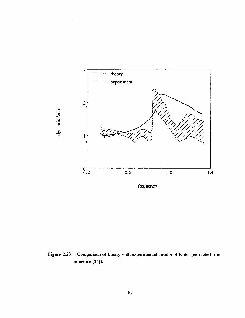
O
t)
3
2
theory
........ experiment
i i i i I
v.2 0.6 1.0 1.4
frequency
Figure 2.23. Comparison of theory with experimental results of Kubo (extracted from
reference [24]).
82

measured for eight different teeth pairs and D L spectrum computed using the
analytical solutions of Section 2.4. Here, at most of the frequencies, our predictions
are not within the measured envelope, but the transition frequency and the amplitude
at the jump discontinuity are predicted accurately. There might be several reasons for
the discrepancy including the usage of D L instead of D S, the validity of the
computer model used to calculate _(t'), insufficient knowledge of some system
parameters such as profile modifications, and the assumptions made in developing
our theory such as the time invariant mesh stiffness. Therefore the experimental data
is not exactly analogous to our analytical predictions even though a satisfactory
agreement is found. Obviously our theory should be refmed in order to obtain a
better agreement with Kubo's data; for instance, time-varying mesh stiffness may be
included.
2.8. COMPARISON OF EXCITATIONS
2.8.1. Internal versus External Excitation
First, we assume that only one type of excitation exists at a time and compare
the frequency response characteristics of the system due to the internal static
transmission error sinusiodal excitation Fi(t) given by equation (2.5) with the external
sinusoidal excitation Pc(t) given by equation (2.4). The comparison is based on the
analytical solutions which are constructed in Section 2.4 for equation (2.5) and in
Reference [33] for equation (2.4). In the case of internal excitation, the amplitude of
2the alternating force has a flh term which makes the alternating force amplitude
2frequency dependent. This amplitude Fah[_ h is smaller than Fah for f_h<l and
greater than Fah when i2h>l. Hence the overall alternating force amplitude ratio
83

F m / F ahf_2h varies with f_h even though F = F m / Fah is kept constant. In the
^case of external excitation, the force amplitude ratio F=Fm/FaT is frequency
independent.
Figures 2.24 and 2.25 compare the frequency responses for four values of
given Fm=0.1, f_h=D,T=f_ and _--0.05. When _ is sufficiently large, say _ >10,
only case I solutions corresponding to the no-impact (case I) exist. Accordingly both
excitations result in the linear system responses which are close to each other for
f2<1; but for f_>l there is a difference which grows with increasing frequency fi as
^shown in Figure 2.24a. When F is reduced to 2, both case I and case II regimes
exist; the difference between two excitations is again significant at higher _2 as shown
in Figure 2.24b. The transition frequencies also differ, and a larger range of dual-
valued solutions is seen for equation (2.5). Case III solutions are witnessed at lower
A
values of F (1 and 0.5) as shown in Figures 2.25a and 2.25b. While equation (2.5)
always has a case I regime at low f_, equation (2.4) does not produce case I atA
F --0.5. Another important observation from Figures 2.24 and 2.25 is that up to two
steady state solutions are seen in the extemal torque excitation case; conversely as
many as three solutions are found for the geared system excited by the static
transmission error.
2.8.2. Periodic or Combined Excitation
The approximate analytical solutions given in Section 2.4 axe constructed only
for a single harmonic internal excitation term _(t') or Fi(t). However, in the real
geared systems, [(t-) or Fi(t) is a periodic which can be represented by a fourier
series of the fundamental frequency _h" Therefore, it is necessary to consider the
84

0.15
0.I0
0.05
(a)
m transmission error excitation
'_ extemal torque excitation
t J i i I .) i i i I i | i ,
0.5 1.0 1.5
frequency
u
(b)
0.50 [_ transmission error excitation
[] external torque excitation
l• s ann_
I i/ "°,
l . , * . , . . a , i , *
0"000.0 0.5 1.0 1.5
frequency
Figure 2.24. Comparison of the frequency response due to the extemal torque excitation
given by Comparin and Singh [33] and the static transmission error excitation;A A
4=0.05, Fro=0.1, Dh=_ T and a) F=10, b) F=2.
85

3
28
°+,,4
(a)
-- transmission error excitation
a extemal torque excitation
, " !
_.0 0.5 1.0 1.5
frequency
4
3
2
0.0
(b)
-- transmission error excitation
o external torque excitation
ooooooOoO _°°
, t , , | , I , i ,
0.5 1.0 1.5
frequency
Figure 2.25. Comparison of the frequency response due to the external torque excitation
given by Comparin and Singh [33] and the static transmission error excitation;A A
4=0.05, Fro=0.1, g2h=K2T and a) F=I, b) F=0.5.
86

higher harmonics of Fi(t) besides the fundamental component which is already
included in the analysis. On the other hand, both external Fe(t) and internal Fi(t)
excitations may exist simultaneously. These two cases require that F(t) in equation
(2.3) be reformulated as follows
F(t)= Fro+ Fe(t) + Fi(t)= Fro+ FaT j sin (jflTt + 0Tj)j=l
k 2
+ Y_ (Jnh) FahjSin(Jf_ht +0hi) (2.20)j=l
In order to construct analytical solutions of this equation, we must investigate
the applicability of the principle of superposition, which would consider first each
excitation separately and then superimpose the corresponding responses to generate
the overall frequency response. Two cases are considered and the analytical results
based on the principle of superposition are verified through digital simulation.
Consider only the static transmission error excitation Fi(t) in equation (2.20)
3with 3 harmonics, i.e. Fe(t) and F(t)= Fm + _ (jflh) 2 FahjSin(j_ht +_hj). The
j=l
amplitudes of the harmonics are selected to be Fahl=0.05, Fala2=0.02 and Fald--O.01,
and the mean force Fro=0.1. First each excitation component is considered separately
without paying any attention to the phase angles and the frequency responses are
obtained using digital simulation as shown in Figure 2.26. Second, all there
excitations are included simultaneously and the overall response is compared with the
previous solutions in Figure 2.26. The frequency response due to each harmonic of
87

the excitation is very close to the overall solution around the resonance peaks
governed by that harmonic. When all of the solutions corresponding to each
harmonic are added algebraically by also considering the phase angles, the overaU
response improves as shown in Figure 2.27. This response is in the form
3
qa(t) = _ qajsin(f_ht +Ohj) where qaj is the altemating displacement when only
j=l
the j-th harmonic is considered. Figure 2.27 suggests that the principle of
superposition can be applied to a gear pair with backlash provided that the excitation
frequencies are sufficiently far apart from each other. In the case of periodic static
transmission excitation, this is valid as all excitation frequencies are at least f_h apart.
Now, the principle of superposition, which has been already verified by digital
simulation, can be used to obtain the approximate analytical solutions per Section 2.4
when the periodic forcing function is considered. Figure 2.28 shows the analytical
frequency response curve for Fro=0.1, Fahl=0.05, Fah2=0.02, Fah3=0.01 and
_=0.05. Here the jump discontinuity is seen only at the peak flhl governed by Fatal
since Fm/Fah 2 and Fm/Fah 3 are both sufficiently high so that no tooth separation
occurs at Oh2 and fib3, respectively. However, the jump phenomenon can also be
seen at the higher harmonics depending on the force ratios Fm/Fahj, j ;_ 1 and _ in
accordance with the results of Section 2.6. The same concept can be applied to the
superharmonic components of the external torque excitation of equation (2.20)
provided Fahj=0.
The principle of superposition is now extended to the case where both intemal
Fi(t) and external Fe(t) sinusoidal excitations exist simultaneously as given by
equation (2.3) provided that the excitation frequencies flh and O T are not close to
each other. In a real geared system, O h is much higher than D, T which implies that
88

.a
0.4
0.3
0.2
0.1
iru_t 3 harmonics simultaneously
1st harmonic
2nd harmonic
3rd harmonic
frequency
Figure 2.26. Comparison of the frequency response qa due to first there harmonics of the
static trancmission error for the cases when the harmonics are considered
simultaneously and separately; Fro=0.1, 4=0.05, Fahl=0.05, Fah2=0.02 and
Fah3--0.01. These results are obtained using digital simulation.
89

0.4
0.3
0.2
0.1
........ O .......
first 3 harmonics simultaneously
principle of superposition
D.,°
0.4 0.80"0.0 1.2
_equency
Figure 2.27. Comparison of digital simulation results obtained by using the principle of
superposition and b'y considering all three harmonic excitations applied
simultaneously; Fm=0.1, _--0.05, Fahl=0.05, Fah2=0.02 and F_3--0.01. In
this case, phase angles are included in the superposition.
9O

0.4
0.3
0.2
0.1
0.4 0.8 1.2
frequency
Figure 2.28. Comparison of the frequency response qa due to trtrst three harmonics of the
static transmission error. This curve is based on the principle of
superposition applied to the analytical solutions which have been constructed
by the method of harmonic balance; Fro--0.1 , _=0.05, Fahl--0.05, Fala2=0.02
and Fala3=0.01.
91

.2
0.4
0.3
0.2
0.1
externalexcitation
I internal_------I J' excitation
Ii
I0.0 .....
v.0 0.4 0.8 1.2
frequency
Figure 2.29. Frequency response qa due to both the external torque and the static
transmission error excitations. This curve is based on the principle of
superposition applied to the analytical solutions which have been constructed
by the method of harmonic balance; Fm=0.1, 4=0.05, Fah=0.05, FAT=0.05,
_"_h=2_T .
92

the principle of superposition should be suitable for this case. Figure 2.29 illustrates
the frequency response solutions due to the fundamental harmonic component of both
excitations for Fro=0.1, Fahl=FaTl=0.05, _=0.05 and by assuming that _h=2_T .
Here, the jump discontinuity is seen at two frequencies. However, when fl h --"_ T
or when one of the superharmonic peaks of Fi(t) coincides with the resonant peak
governed by Fe(t), the principle of superposition will no longer be applicable. In
such cases, we will use the digital simulation as the analytical interpretation of these
cases is yet to be explored.
2.9. CONCLUSION
This analytical study on the non-linear dynamics of a spur gear pair with
backlash as excited by the static transmission error has made a number of
contributions to the state of the art. First, difficulties associated with the digital
simulation technique have been resolved as multiple steady state solutions at a given
frequency can be found provided the entire initial condition map is searched. Second,
new frequency response solutions for the gear pair have been constructed using the
method of harmonic balance. "third, our mathematical models have been validated as
these compare well with two previous experimental studies and the key parameters
such as the mean load, mean to alternating force ratio, damping and backlash have
been identified. Forth, the chaotic and subharmonic resonances are observed if the
mean load is too small for a lightly damped system. Fifth, mathematical conditions
for tooth separation and back collision have been established which are compatible
with available measured data. Sixth, the periodic transmission error excitation case
has been analyzed using the method of harmonic balance in conjunction with the
principle of superposition. Finally, on a more fundamental note, our study enriches
93

the current literature on the clearance non-linearity or vibro-impact systems as the
governing non-linear differential equation is different from the conventional single
degree of freedom system formulation.
94

CHAPTER 111
NON-LINEAR DYNAMIC ANALYSIS A GEARED ROTOR-
BEARING SYSTEM WITH MULTIPLE CLEARANCES
3.1. INTRODUCTION
Mathematical modeling of geared rotor-bearing systems, being an essential step in
designing quiet and reliable power transmissions, has been the subject of numerous
studies over the past few decades. Most proposed dynamic models, as reviewed by
Ozguven and Houser [14], are essentially linear. However in several cases, it has been
experimentally shown that the geared systems exhibit non-linear behavior [27-29,35].
For instance, vibro-impacts are observed in a lightly loaded transmission with gear
backlash or loose bearings [30,31,34]. Accordingly, we must develop non-linear
mathematical model of the geared system - this is main focus of this chapter with
emphasis on the clearance type non-linearity in gears and rolling element bearings. In
Chapter H we had considered the single degree of freedom non-linear model of a spur
gear pair with backlash and investigated the effects of system parameters on the
vibrations and chaos excited by the static transmission error. Applicability of the
harmonic balance method and digital simulation technique to the solution of the steady
state response has been demonstrated, and difficulties associated with the digital
simulation technique when applied to such systems governed by stiff non-linear
differential equations have also been resolved in Chapter II.
Although there is a vast body of literature which considers a single degree of
freedom system with clearances, as reviewed earlier in Chapter II, studies on the multi
95

degree of freedom vibro-impact systems are very limited. For example, Galhoud et.al.
[52] considered a two degree of freedom translational system with a gap and found the
forced harmonic response using the piecewise linear technique. Winter and Kojima
[53] also used the same technique to study the geared systems with backlash.
However, it should be noted that the piecewise linear technique can not predict several
non-linear phenomena such as subharmonic and chaotic responses since it employs the
assumption that both impact and no-impact regimes "are repeated in an identical manner
once every period of excitation" [52]. Kucukay [35] developed an eight degree of
freedom model of a helical gear pair with backlash to include the rocking and axial
motions of rigid shafts and radial deflections of linear bearings. Lin et.al. [38] included
motor and load inertias in a three degree of freedom torsional model. Both of these
studies employed the digital simulation technique, but did not consider a number of
issues of primary concern in non-linear system such as the existence of multiple steady
state solutions, their dependence on initial conditions, subharmonic, quasi-periodic and
chaotic responses, etc. A few of these issues have been addressed by Singh et.al [34]
on the gear rattle problem. Comparin and Singh [54] have also used the digital
simulation, analog simulation and harmonic balance method to analyze coupled impact
pairs assuming that the modes are "weakly coupled", which allows the system to be
represented by a combination of single impact pairs. They included only the low
frequency external torque excitation and found the steady state frequency response at
the primary resonance. This solution has then been used to analyze the neutral gear
problem in more detail [55].
The other two groups of studies which consider multi-degree of freedom systems
with continuous non-linearities [56-61] and periodic excitations due to mesh stiffness
variations [29,62], will not be addressed here since their responses are significantly
96

different from the clearance non-linearities as discussed by Comparin and Singh [33].
The literature on chaotic vibrations and roiling element bearings will be discussed later.
3.2. PROBLEM FORMULATION
3.2.1. Scope
Figure 3.1 shows the generic geared system considered in this study. It consists
of a spur gear pair mounted on flexible shafts which are supported by roiling element
bearings assembled in a rigid gear box. Since the shafts and bearings are compliant,
our single degree of freedom model of spur gear pair which assumes fixed gear centers
is obviously not suitable. Instead, a three degree of freedom non-linear model as
shown in Figure 3.2a is considered. It includes equivalent stiffness and damping
elements representing the shaft and the bearings. The corresponding linear model has
been found to be sufficiently accurate when compared with a f'mite element model for
eigen solutions provided that the gear dynamic response (mesh force, dynamic
transmission error, etc.) is of major concern. Gear backlash and radial clearances in
bearings are defined analytically. An approximate non-linear bearing model is also
proposed. Applicability of both analytical and numerical solution techniques to this
problem is investigated. Several key issues such as non-linear modal interactions and
differences between internal static transmission error excitation and external torque
excitation are discussed. Parametric studies are conducted to understand the effect of
system parameters such as bearing stiffness kbi to mesh stiffness k h ratio
1_= kbi/'k h , ahemating to mean force ratio Fa/F m and radial bearing preload to mean
force ratio Fb/F m on the non-linear frequency response. A criterion is used to classify
the steady state solutions, and the conditions for chaotic, quasi-periodic and
subharmonic steady state solutions are determined. Two typical routes to chaos
97

gear box
driving shaft
pinion
driven shaft
gear
roilingelement
bearings
Figure 3.1. Generic geared rotor-bearing system.
98
observed on a geared system are also identified. Finally, our formulation is verified by
comparing predictions with measurements [27].
3.2.2. Physical Model and Assumptions
The three degree of freedom non-linear model of the geared rotor system with
gear inertias Ig I and Ig2, gear masses mg I and mg2, and base circle diameters dg I and
dg 2, as shown in Figure 3.2a, is considered here. The gear mesh is described by a
non-linear displacement function fh and viscous damping ch. Friction forces at the
mesh point are assumed to be negligible [18]. Thus the transverse vibrations in the
pressure line direction are uncoupled from the vibrations in the direction perpendicular
to the pressure line. Bearings and the shafts that support the gears are modeled by
equivalent elements with viscous damping coefficients Cbl and Cb2 and non-linear
springs defined by force-displacement functions fbl and fb2. The effects of the prime
mover and the load inertias are not considered assuming that these inertial elements are
connected to the gear box through soft torsional couplings. Further, we assume that
the system is symmetric about the plane of the gears and the axial motion (parallel to the
shafts) is negligible. Like the spur gear pair model of Chapter II, both low frequency
external excitation due to torque fluctuations and high frequency internal excitations due
to the static transmission error [(i) are considered in the formulation. Input torque
fluctuation is included, but the output torque is assumed to be constant, i.e.
Tgl(i) = Tglm + Tgla(i) and Tg2(i) = Tg2m. External radial preloads _ol and Fb2 are
also applied to both rolling element bearings.
99

3.2.3. Equations of Motion
Equations of coupled transverse-torsional motion of the non-linear geared rotor-
bearing system shown in Figure 3.2a are
mgl Yg'l + Cbl Ygl + Ch(X' + Ygl - Yg2 - e') + kbl fbl(Ygl)
+kh fh(x+ Ygl- Yg2 -e) = -F_ol (3.1a)
mg2 Yg2 + Cb2 Yg2 - Ch(X'+ Ygl - Yg2 - e')+ kb2 fb2(Yg2)
-kh fh(x + Ygl- Yg2 -e)= F_b2 (3.1b)
mcl Ch(X'+Ygl-Yg2-e')+khfh(X+Ygl-Yg2 e)=Fm+FaT(t)(3.1c)
1
mcl= Id2..___[+ d22 I ;
[4Igl 4Ig2)
(3.1d,e)
Fm= 2%1m = 2%2m ; FaT(i') = mcl%la0)
dgl dg2 2Igl(3.1f,g)
Here, ( )' means derivative with respect to time t, Ygi and 0g i are the transverse and
torsional displacements of the i-th gear (i=1,2), rncl is the equivalent gear pair mass,
Fm is the average force transmitted through the gear mesh and FaT(t) is the fluctuating
force related to the extemal input torque excitation. Equations (3.1a), (3.1b) and (3.1c)
are simplified further by def'ming below a new variable _(t) which is the difference
between the dynamic transmission error and the static transmission error _(t).
100

pinion Ogl
mg 1 ,I !0 'dgl_
..... excitationS(t)roumg eJementbearing model
including shaft _
(a)
\
)_Og2
mg2 ,Ig2,dg2
pinion Ogl
excitationS(_) __ Og2
_" rag2 ,Ig2.dg2(b)
Figure 3.2. Non-linear models of the geared rotor-bearing system; a) three degree of
freedom model, b) two degree of freedom model.
101

_(i) = _(i) + y$1(i) - yg2(i)- E(i) ; (3.2a)
mP, Omg2
k-mcl mcl mclJ[ p"(i)J L0
o Chl[Yb(i)]Cb2 - Ch_Yg2(t) I
o ch j[ p'(i),l
t0 kh J[ fh(P) J Fm - mole' (i)+ FaT(i)
A dimensionless form of equation (3.2b) is obtained by letting
Ygi(i) = Ygi(i)/bc, P(i)=P(i)/bc, tOn = 3]kh/mcl, tobi = 4kbi/mgi 0=1,2) and
t = toni where b c is the characteristic length. Here, we consider harmonic excitation for
both E(i) and FaT(i) as E(i)--fisin(_hi +Oh), F.T(i) - FaT sin(_T i +OT) where _h
and _T are the fundamental excitation frequencies of internal displacement and external
torque fluctuations, respectively. Further, define dimensionless excitation frequencies
_"_h-" _h/On arld GT = _T/COn tO yield the following dimensionless governing
equation ofmotion.
1 oo]V.,,,,1 F,,o0 l OH_,_,_/+_/o _=-_23_'g2(t)_'-I 1 Ij[ i_(t ) j Lo o _33J[ t)(t) J
lqi 0 lcl3/1fb2(Y.2) f {F(t));+ K22 - K23 =
0 1 j{ fh(p) J
(3.3a)
102

{F(t)} = {F}m + {F(t)}i + {F(t)}e
I°l {:= + 0 sin(flht + _h ) +
[Fm J [Fah_2J FaT
' sin(flTt + OT );(3.3b)
_ii = Cbi ," _i3 = Ch , i=1,2; _33 = Ch2mgitOn 2mgimn 2mcl_n
; (3.3c,d,e)
Kii = _v4;2 K i3=m
tOn mgi
Fbi i=1,2;
Fbi- mgibct.O 2'(3.3f,g,h)
= Fm . "e FaT = mclbFaTo)2 (3.3i,j,k)Fm mclbc_2 ' Fah = bc ;
where Fbi (i=1,2) and Fm, are the dimensionless components of the mean force vector
IF} m, and FaT and Fah pertain to the altemating extemal excitation {F(t)} e and internal
excitation {F(t) }i force vectors, respectively.
3.2.4. Modeling of Non-linearities
The non-linear displacement functions fbi(Ygi), i=l, 2 and fh(P) in equation
(3.3a), which represent the bearing radial and gear mesh stfffnesses, respectively,
should be defined explicitly before solving the non-linear equations. Here, fh(P) is,
detrmed as a clearance type dead space function with a backlash 2b h and linear time-
invariant mesh stiffness of one, in the dimensionless form
103

F-, the i.-tl:ioli_.__..... i; .......... k_a_, rad:s_._ ........ ,_.. ' t' ,,,o, ' ,_ie,.-,-,_, '-..... ; .... - - _.,,c_. _ ,;e_s,-_s v,__-:p_ac._ment };g_
relationship on(_:_ _;_e -:l_;i'.c !oa, li_g _- ......... ' " " '
[:-i_ + \11
}; [ , _ 1 r :: (- {1}_; -- -- bb _ i cos(:{,; ": > '
(): - b_,. <vei < bbi (3.5)
, F'-, [i- I . ,_r_.
_': y__i < --bbi
w,he[e kii i-: )!_e r,_e_ ::¢_:_t:_.:_ .'_ ff.g:-->:, ".g _s _I_;-.,oigu__,a _,v._>;iri.,m<:f the r-th rolling
.... : _ <!earaa_ce of the i:+h _,,=_g-,- n is the power of the
non-linear force di:;pia.cemen: re!ati_m_hip (n=l.5 f_, bali be,'u'ings and n-10/9 for
roller bearings) and 1t is the total number of rolling elements m contact under loaded
conditions. Now the dimensionless bearing displacement .function fbi(Ygi) of equation
(3.3a) is obtained from equation (3.5} as
: 04 ORIGINAL PAGE ISOF POOR QUALITY

1 YgiC°SCCr- bc J > bc
Fy.___i= ["/ bbi <Ygi < 'fbi(Ygi)= ktibc 0; bc _ .
/-r_lOYgilCOSOC r -bbi/n _c !bc j cosCCr; Ygi <-
(3.6)
Figure 3.3 shows the non-linear function fgi(Ygi) for a roller bearing with n=10/9,
kt=lxl08 N/ml0/9, total number of rollers Z=15 and bb--O.01 mm. In Figure 3.3, we
note almost a line:,: __"_tionship for large displacements, say Ygi>3bbi_c . Since the
degree of non-linearity is not very significant, equation (3.6) can be approximated by a
piece-wise linear function, similar to fh(P) given by equation (3.4), in order to simplify
the analysis considerably. Figure 3.3 also illustrates two linear approximations A and
B beyond the clearance for fbi(Ygi) in the form
fbi (Ygi) =
bbi. bbi
Ygi- b----_' Ygi > ---bc
bbiO; bbi <Ygi <----
bc bc
bhi bbiYgi + _; Ygi < ---
bc bc
(3.7)
Note that both approximations A and B differ in clearances bbi A and bbi B but have the
same slope as the exact beating stiffness curve for Ygi>3bbi/bc, i=1,2, which is unity in
the dimensionless form. The validity of these approximations will be given later.
105
OF POOR QUALFFY

4
approximation B
approximation A'
-4 0 4
displacement
Figure 3.3. Exact and approximate bearing deflection functions.
106

3.3. CORRESPONDING LINEAR MODEL
As a limiting case, equations of motion of the corresponding linear system are
obtained by substituting fbi(Ygi) = Ygi, for i=1 and 2, and fh(P) = P in equation (3.3a)
1 1J_ ii(t ) I
0 _13 ][)'gl(t)]
0 _33_H l_(t) j
[KII 0 KI3 ][Ygl(t) /
+[_ K22--K23_Yg2(t'I=0 K33/[ p(t) J
{F(t)} (3.8a)
or in the matrix form with (q(t) } as the displacement vector
[M]{q(t)} + [C]{q(t)} + [K]lq(t)} = {F(t)} (3.8b)
where the mass [M], damping [C] and stiffness [K] matrices are all positive definite.
These matrices are asymmetric due to Ygl and Yg2 terms in the last row of matrix
equation (3.8a). For this linear system, the mean and alternating components of the
motion can be separated by letting Ygi(t)=Ygim+Ygia(t), i=1,2 and p(t)--pm+Pa(t).
Hence, equation (3.8a) is rearranged in terms of the alternating motion as
[M]lqa (t)l + [C]{qa (t)} + [K]lqa (t)l = {F(t)}i + {F(t)le (3.9)
The natural frequencies _r and the modes {Vr} are calculated by considering the
corresponding eigen-value problem. The forced harmonic vibration response is then
107

obtainedby themodalexpansiontechniquein thefollowing form
3 {_I/r}{l]/r }T Fah_2h Sin(/k"_ht + ¢_h)
{qa(t)}=r=l y" [(_-_2h)+j_hCr]
3 {_tr }{_l/r}T F t"_2
+ Z [_(Or2 2 aT T_=1 - _'-_T)+ j_TCr ] sin(t-_Tt + _T );j = x/-i (3.10a)
1 {1; r=sCr=_-_-_ {lltr}T[C]{_s}; 5rs= 0; r;es (3.10b)
Table 3.1 shows the natural frequencies of the three degree of freedom linear
system given by equation (3.9) and the ones found by finite element method for three
different l_=kbi/k h values with mgi=l kg, Igi=0.0008 kg/m 2, dgi=0.08 m,
_ii=0.01, _i3=0.0125, _33=0.05, i=l, 2 and kh=2xl08 N/m. As evident from Table
3.1, the three degree of freedom and finite element models [15] result in virtually the
same natural frequencies. This concludes that the three degree of freedom model is
indeed suitable for the geared-rotor bearing system. The first _I and third VIII natural
modes are coupled transverse-torsional modes while _1/ii is purely transverse type [15].
The second natural mode _tll is not excited by _(t) in this particular case, since the gear
ratio yg=dgJdg 1 is one for a symmetric pair. Therefore only two peaks should exist in
the frequency response spectrum which will be presented in Section 3.5.
108
ORIGt_AL PAGE IS
OF POOR QUALWY

Tab! c 3. ! Natural fre.',., _er_':ies_ .,:'-r_be ............(_._::,_,_.i:,i,:'g.';"" tl:ree_ degree of freedom (3-
DC, F) " .....
k::kbi/k h
1 _ 10
3oDOF/FEM
fi.;S] I IADSV_! --:_:-
torsional cnup[: ":
purcly _rans,'mse (_1_ 0.753.4? 7c'5
second tr_msverse- o}i!a (_,gk('/_,_:::_O
torsiop.al coupled
Finile E]e:nen! Method (I-_M ! {>_m Retere_ce I15].
1.475/1.560
_..96:_.868
I , _ai
3.4. TWO DEGREE OF FREEDOM SYSTEM STUDIES
3.4.1. Equations of Motion
As a first example, we reduce the three degree of freedom transverse-torsional
semi-definite model to a two degree of freedom non-linear model. This is obtained by
clamping one of the gear centers as shown in Figure 3.2b, i.e. one of the transverse
displacements is assumed to be zero, say Ygl=0 which physically corresponds to a
system with one gear gl mounted on a rigid shaft which is supported by very stiff
bearings while the other gear g2 is assembled with compliant lumped shaft and
bearings. Equations of motion of the reduced order system are obtained from equation
(3.3a) by letting ygl=0.
1JL i (t) J JL p(t) j
o 1 Jt fb(P) J
The intent here is to simplify the physical system in order to investigate several
key issues in depth. Specifically, the objectives are to: a) justify using approximate
bearing models proposed in Section 3.2.4 by comparing the frequency responses
excited by _(t), b) show applicability of the harmonic balance method (I-IBM) to solve
non-linear system equations and compare its predictions with the results yielded by the
digital simulation technique, c) study interactions between system non-linearities for
both weakly and strongly coupled modes, and d) compare the steady state frequency
response spectra due to internal static transmission error excitation {F(t)}i and external
torque excitation { F(t) }e.
110

3.4.2. Solution
Both analytical and numerical solution techniques which we have used
successfully for the spur gear pair problem are employed again to solve equation
(3.11). First, approximate analytical solutions are constructed using the harmonic
balance method [33,51 ] with only the bearing non-linearity assuming no gear backlash,
i.e. bh--O or fh(P)--P. For the harmonic excitation given by equation (3.3), we assume
p(t)=pm +Pasin(f_ht+_p); Yg2(t)=Yg2m +Yg2asin(f_ht+_g2) (3.12a,b)
where subscripts m and a represent mean and ahemating components of the steady state
response, and Op and #g2 are the phase angles. The non-linear bearing function is
approximated as
fb2 (Yg2) = NmYg2m + NaYg2a sin(_ht + 0g2 ). (3.13)
where Nm=Nm(Yg2m,Yg2a) and Na=Na(Yg2m,Yg2a) are the describing functions which
are given in Chapter II; these need to be defined for each impact regime (no impact,
single sided impact, double sided impact). Governing frequency response equations
are obtained by substituting equations (3.12) and (3.13) into equation (3.11) and
equating the coefficients of like harmonics:
+ ]ngFa Pa = ._- ;
(3.14a)
11I

A = (-a3K23AI + 4a4;22;23 + A2 A2 + 4a_;22A2)2
2 2+(-2a3G2K:3- m3 E3A + mh 33A + 8a G:;33) ; (3.14b)
AI = K:22Na -a2; A2 =l-a2 ; pro=Fro • (3.14c,d,e)
_¢223+ (2_b_2 3)2 ]1/2Yg2a = (K23AI _ 4_2_22_23)2 + (2.Qh_22K23 + 2f/h_23A 1)2; (3 i4f)
Fb2 + K23P m
Yg2m = K22N m (3.14g)
The overall frequency response is obtained by solving equation (3.14) numerically for
each impact regime separately.
Second, the digital simulation technique is used to solve equation (3.11) for no
gear backlash. A 5th-6th order variable step size Runge Kutta numerical integration
algorithm [50], which has already been employed successfully in solving similar
problems, is used here. Figure 3.4 compares frequency response spectra obtained
using the harmonic balance method and digital simulation. Although both methods are
in a very close agreement for the case considered in Figure 3.4, one should be aware of
the following: (i) several problems may exist in the application of the numerical
integration method to the clearance type problems, hence caution must be exercised.
and (ii) the harmonic balance method is incapable of predicting chaotic and
subharmonic responses. Accordingly for further analysis, we will use only the digital
simulation technique.
112O,_i_!{2fiLP_GE' IS
OF" POOR QU.A,LrI'Y

a)
-3
.,,.q
2
I
J
!.13
0
-° digital simulation
^ HBM
i
_o_ _
1 2
b)
"3
.a
-_ digital simulation
HBM
t_
&
i
0__;_ ='_,3 1 2
frequency
b
1_1_ "13-_,.la _, o o o Q Q Q
Figure 3.4. _.ompans_ n of hamaonic balance method and digital simulation ;echnique:
Fm=l.0, Fah=0.5, Fb2=O, bh=0, bb2=bc, _33=0.05, _23=0.0125,
¢22=0.01, 1_= 1 ; a) Yg2a versus _h, b) Pa versus f_h-
113
3.4.3. Validation of Non-linear Bearing Model
We examine the validity of two approximations for fbi(Ygi), as suggested in
Section 3.2.4 and shown in Figure 3.3, by assuming bh----0 and FAT--0. Equation
(3.11) is solved using the digital simulation technique, given Fm=l.0 , Fah=0.05,
Fb2--0, {22--0.01, {33=0.05, 423--0.0125 and ;c22=tc23=0.25, for three bearing models
(exact, approximations A: bb2A=bb2=bc, approximation B: bb2 B =1.63bb2=1.63bc).
Figures 3.5a and 3.5b compare Yg2a versus £"_h and Pa versus t'lh spectra for all three
bearing models. Both approximations are in a very close agreement with the exact
bearing model over the entire frequency range. The frequency and the amplitude of the
jump at the first peak is predicted accurately by both approximate models. Hence we
conclude that the approximate piecewise linear model can be used for a bearing without
losing any accuracy and the dynamic behavior is not sensitive to the minor variations in
bearing clearances bbi.
3.4.4. Non-linear Modal Interactions
Although both natural modes of the corresponding linear model are transverse-
torsional coupled modes, first mode WI is more dependent on transverse vibrations than
the second peak. Accordingly, it is expected that bearing non-linearities should affect
the f'trst peak directly while gear backlash should dominate the second peak in Figure
3.4. The validity of this claim depends on the nature of non-linearities and system
parameter values, as illustrated below.
First, a set of parameters is selected so that natural frequencies 0)1 and o_Ii of the
corresponding linear system are far away from each other: o)i----0.437 and o)iI=1.144
for _:22=0.25, _:23---0.25, _22=0.01, _23=0.0125, and 433=0.05. Frequency response
characteristics of the system with a forcing function, Fm=l.0 and Fah=0.5 are evaluated
114

a)
00
exact
................ approximation A
a approximation B
1 2
b)
6 ] exact
.................. approximation A
approximation B
00 1 2
_equency
Figure 3.5. Comparison of frequency responses obtained by using the exact and
approximate bearing displacement functions given in Figure 3.3;
Fm=l.0, Fah=0.5, Fb2=0, bh=0, bb2=bc,_33=0.05, _23=0.0125,
_22=0.01, f_ = 1; a) Yg2a versus flh, b) Pa versus f_h.
115

for the following three cases: a) no gear backlash, bh=0, non-linear bearing, b,b2=bc: b)
gear backlash, bh=10b o linear bearing, bb2--0; and c) gear backlash and non-linear
bearing with bh=10bb2=10b c. In the last pa'o cases, gear backlash is _aken to be i0
times the bearing clearance as it is a typical order of magnitude value for many geared
rotor systems supported by roller bearings. Figures 3.6 and 3.7 show the frequency
responses, Yg2a versus 1-_h and Pa versus O h respectively, for all three cases given
above; also superimposed is the linear frequency response curve for comparison
purposes. As shown in Figure 3.6a and 3.7a, a jump discontinuity is observed at the
first peak only for case a. in the case with only gear backlash non-lmearity, jump is
seen at the second peak while the first peak is continuous as shown in Figures 3.6b and
3.7b; this supports the claim of torsional mode dominance of the second peak. Finally,
when both non-linearities are included sinmltaneously, both peaks become non-linear
as shown in Figures 3.6c and 3.7c. For such a system, natural modes are essentially
"uncoupled" mad the inter.actions between component non-linearities are negligible. In
sun'unary, for case a of Figures 3.6a m-,d 3.7a, a linear model can be used to predict the
frequency responae beyond .coI , say t2h> 0.6. Similariy, a linear model could be
suitable for case b for tlh<0.8 as shown in Figures 3 6b and 3.7c. But for case c, a
linear model is suitable only tar away from the resonances.
Second, choose a dataset, say K22=0.64, K23=0.10 , _22=0.01, _23=0.0125, and
_33--0.05, such that two natural frequencies for the corresponding linear system are
brought closer to each other: o1=0.720, 01i=1.101. We again consider the same cases
a, b and c and compare the frequency response for Fro=2.0 and Fah=0.5 in Figures 3.8
and 3.9. Here, each non-linearity affects both modes, resulting in jumps at each peak.
Therefore, for this set of parameters, modes are considered to be "coupled" because of
dynamic interactions. Accordingly both non-linearities must be included
i16
O,',,'_;,":'_J P£GE IS
OF POOR QUALITY

a)
b)
.a
2
00
III
o II
°11
f I
1 2
3IIJ!IfIIIt
I II IJ II
I \ Ao / \\
l °a.
1 2
c)
.2
00
III
II[] II
'a
t
vii " a a
1 2
frequency
Figure 3.6. Yg2a versus _')h plots for the case of uncoupled modes; a) no backlash,
non-linear bearings, b) backlash, linear bearings, c) backlash, non-linear
bearings; corresponding linear response.
117

a) 5.0
b)
o
. 2.5
0.%
! I
:\P
___._n__ / i
1 2
5.0
2.5
0.00
o I I
°° / '\
,,7
1 2
c) 5.0
2.5
0"00 1
/_
I
_o \
i °°o
I
/
frequency
Figure 3.7. Pa versus f_h plots for the case of uncoupled modes; a) no backlash, non-
linear bearings, b) backlash, linear bearings, c) backlash, non-linear
bearings; corresponding linear response.
118

a)
b)
5.0II
IIIIliIt
2.5 J1It
II o
I I 4, aaat :',/ ol o I_ I "o_
o.o____-., i , -........ -
3
o_____j!I 2
c) 6
3
I D
I, I°°Oo
0 1 2
frequency
Figure 3.8. Yg2a versus _h plots for the case of coupled modes; a) no backlash, non-
linear bearings, b) backlash, linear bearings, c) backlash, non-linear
bearings; corresponding linear response.
119

a)
b)
c)
6
3
0
IIInfi o o
fl
fl '_aII a/_
lI a / -_.,
ff #, I "_
rl a
I /
--_--_-- On__ , .
0 1 2
8
[]
° TI4
°o 1 2
6
3
00
IIInII aIIII
II
II __
fl /Jl
,J__,_"g[] ,1 2
frequency
Figure 3.9. Pa versus fi b plots for the case of coupled modes: a) no backlash, non-
linear bearings, l_) backlash, linear bearings, c) backlash, non-linear
bearings; corresponding linear response.
120

simultaneously in the dynamic model.
3.4.5. Internal versus External Excitation
Here we will apply only one type of excitation at a time and compare frequency
response characteristics of the system due to sinusoidal excitations IF(t)} i and IF(t))e
in equation (3.3a). Here, only the bearing non-linearity will be considered assuming
no tooth separation, bh=0. In the case of intemal excitation, amplitude of altemating
component is dependent on flh2 . Conversely, the amplitude of altemating external force
is frequency independent. Therefore, for a constant force ratio Fai/Fm, i=h,T, the
overall amplitude ratio _2hFah/F m for intemal excitation varies with excitation frequency
whereas the overall amplitude ratio FaT/Fro for extemal excitation remains constant
similar to the single degree of freedom model of Chapter I1.
Figures 3.10a and 3.10b compare Yg2a versus f_ and Pa versus _ spectra for
_t=_h=f_, Fm=l.0 , FaT=Fah=0.5, Fb2=0, 422=0.01, 423=0.0125, 433=0.05 and
_:22=_:23=0.25. As shown Figures 3.10a and 3.10b, both excitations yield the same
values at fl=l.0 since Fm/FaT=Fm/_2Fah at t_=l.0. For fl>l the intemal excitation
gives larger amplitudes than the external excitation, but the converse is true for _<1.
Another important difference is that for increasing fi, there are two jumps ( a jump-up
from the no-impact regime to the double sided impact regime at fl=0.3 and a jump-
down from the double sided to the single sided impact regimes at _=0.4) for the
external excitation; but the double sided impact regime is not seen in the intemal
excitation case and only one jump from the no-impact to the single sided impact is
found at f1=0.35.
121

a) 100
10
i
.01
•001 o
intemal excitation
, ................... external excitation/
ff
// ., I
1 2
b) 10
.1
.01
.0010
o°°°°°o°, J°o,°°_
1
intemal excitation.................. external excitation
i
1 2
frequency
Figure 3.10. Comparison of frequency responses due to intemal static transmission
error and external torque excitation; Fm=l.0, Fah=0.5, Fb2=0, bh=0 ,
bb2=bc, _33=0.05, _23=0.0125, _22=0.01, lc = 1; a) YgEa versus _h, b)
Pa versus _h.
122

3.5. THREE DEGREE OF FREEDOM SYSTEM STUDIES
3.5.1. Classification of Steady State Solutions
The steady state response results excited by internal force {F(t)}i at each
frequency _h have been categorized into the following five groups: (i) harmonic or
nearly harmonic solution at the same period tp=2_/_ h as that of forcing function
(period-one), (ii) non-harmonic period-one solution, (iii) subharmonic solution with
period ntp, n>l, (iv) quasi-periodic solution, and (v) chaotic solution (non-periodic,
n _ *_). The solution classification criteria are based on time histories, phase plane
plots, Poincare maps and Fourier spectra [66-71]. Figures 3.11 through 3.15 illustrate
different types of steady state solutions obtained from the three degree of freedom non-
linear model of Figure 3.2a. As shown in Figure 3.11, period-one, non-harmonic
solutions have a non-circular (non-elliptic) phase plane plot and repeat themselves at tp.
Figure 3.12 shows the time histories, phase plane plots and Poincare maps for a 2tp
subharmonic solution. In this case, the Poincare map consists of two discrete points.
Similarly, the 6tp (uhra)subharmonic response has six points on the Poincare map as
shown in Figure 3.13. Figure 3.14 illustrates a typical quasi-periodic response
(combination oscillations) which consists of two or more "incommensurate"
frequencies [66,67]. Quasi-periodic solutions result in closed orbits on the Poincare
map as shown in Figure 3.14c. The chaotic responses which are defined by a non-
periodic time history and as many points as the number of cycles considered in the
analysis on the Poincare map are illustrated in Figure 3.15. Figures 3.16a-e show the
FP-T spectra corresponding to the time histories given in Figures 3.11 to 3.15. For
period-one non-harmonic solution of Figure 3.11, corresponding spectrum has peaks at
me where co is the fundamental frequency and m is a positive integer, as shown in
Figure 3.16a. The ntp subharmonic solutions contain peaks at the frequencies mo_/n.
123

For instance, spectra of the 2tp and 6tp solutions of Figures 3.12 and 3.13 have peaks
at frequencies mo_/2 and mo_/6 respectively in Figures 3.16b and 3.17a. The quasi-
periodic solution of Figure 3.14 consists of two fundamental frequencies oaI and o)2 at
a ratio to I/(o 2 --8 (an irrational number) and there are peaks at the combination
frequencies m(ol+r¢.o2, m,r =0, 5:1,+2 .... Finally, a characteristic broad band
spectrum is obtained in Figure 3.18 when the solution as shown in Figure 3.15 is
chaotic.
3.5.2. Routes to Chaos
In Chapter 1I, we had investigated the effect of mean load F m and damping _ on
chaotic response of a gear pair. It has been shown that chaos typically exists in
lightly damped and lightly loaded gear pairs. Now, two different routes to chaos for
the three degree of freedom system are illustrated.
A. Period-Doubling RouSe to Cha9# ; This consists of a sequence of bifurcations
of the periodic response to another periodic response with twice the period of the
original response due to a change in one of the system parameters [66, 68-70]. Figures
3.19 to 3.23 demonstrates this with a change in excitation frequency fl h given Fro--0.1,
Fah=0.05, Fbi----0 i=1,2, 4! 1=422=0.01,413=423=0.0125, 433=0.05, K 11=822=1.25,
_13=_:23=0.25, bc=b h and bbi---0, i=1,2. At f2h=1.500, with zero initial conditions,
we note a tp harmonic solution in Figure 3.19. This tp solution bifurcates to 2tp
subharmonic solution in Figure 3.20 when l) h is reduced to f2h=1.48. Furthermore at
f2h= 1.44 a 4tp solution is obtained which is further transformed to a 8tp response at
L'_h=1.402 as shown in Figures 3.21 and 3.22 respectively. At _"_h=1.4, however the
steady state solution becomes chaotic as evident from Figure 3.23. Also note from
124

O •
Ygl(t)
--2.
390 t/tp 4 o o
(a)
5 °
_5. ' |
390 t/tp 400
0.5
3'gl(t)
10-2.0
(b)2 °
p(t)
Figure 3.11. A non-haxmonic period-one response; Fm=l.O, Fah=0.5, Fb2=O, bh=0,
bb2=bc, _33 =0.05, _13=_23 =0-0125, _11=_22 =0"01, 1_=5, _h=0.6; a)
time histories, b) phase plane plots.
125

0 °
Ygl(t)
--2°
390 t/tp 4 O0
2 •
p(t)
0390
0.5
_'gl(t)
1.0
/_(t)
-.5 -I.0
-0 5 0 2 0- 2. o -'g"-] (t) - - •
i | •
p(t)
.35
,gl(t)
x
0 °
15(t)
x
x.20 X , , -.6 ' ' '
- 1.1 o., ,,"gl(t _ - 1. o 7 o. 6 p(t) x. 4
Figure 3.12. A period-two subharmonic response; Fm=l.0, Fah=0.5 , Fb2=0, bh=0 ,
bb2=bc, _33=0.05, _13=_23=0.0125, _11=_22--O.01, 1<=5, _')h=0.85.
126
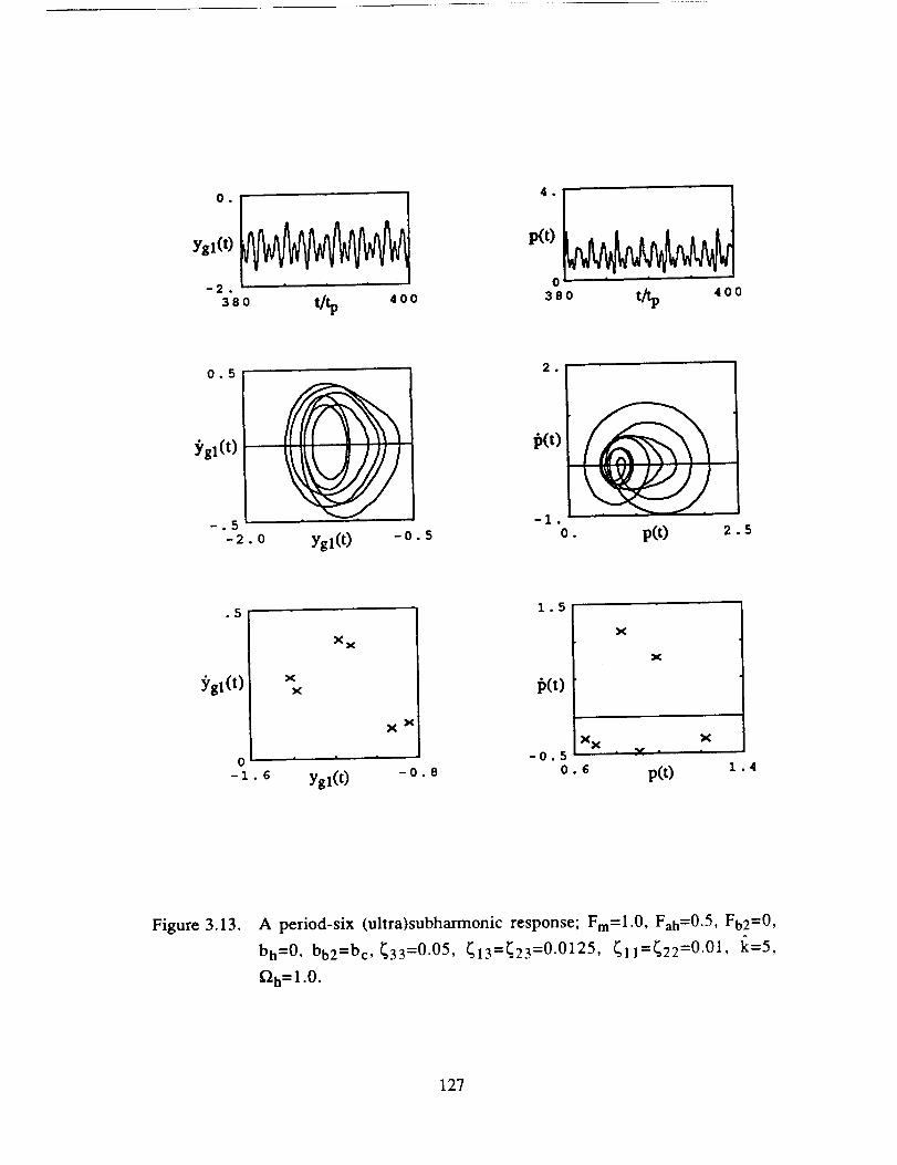
ygl(O
--2.
380 t/tp 400380 t/_p 400
)'gl(t)
2 .
f_(t)
0 • p(O 2.5
.5
$'gl(t) ×x
0-!.6
X X x
x
1.5
lb(t)
X X-0.5
0.6
X x
Xi a v j , [
Ygl(t) -o. 8 p(t) z. 4
Figure 3.13.A period-six (ultra)subharmonic response; Fm=l.0, Fah=0.5, Fb2=0,
bh=0' bb2=bc'_33=0"05' _13=_23 =0"0125, _11=_22=0.01, 1_=5,f_la= 1.0.
127

0 .
Ygl(t)
--2.
380 _p 40O
5 •
380 _ 400
0.5
:ggl(t)
-1.0-2.0
Ygl(t) o. o
2 •
-2°
- 1. O. p(t) 3.
.035
Ygl(t)'
• il
.020 ' ' ' .06 '- 95 - 05
-. 9 9 Ygl(t) " " p(t)0.10
Figure 3.14. A quasi-periodic response; Fm=l.0 , Fah=0.5, Fb2=0, bh=0 , bb2=bc,
433=0.05, _13=_23=0.0125, _11=_22=0.01, i_=5, _h=0.65.
128

S *
m5 ° ....
38o tap 4oo
5 •
pCt)
2. S°
-2 . -5.
- 3. Ygl(t) 2. - 4. p(t) °
0.2
Ygl(t)
0.4
• f (t),,J li- • *
-.2 ' ' -.4
-1.5 _,,vglrt_ o.o -.4 p(t) o.4
Figure 3.15. A chaotic response; Fm=l.O, Fah=0.5, Fb2=0, bh=0 , bb2=bc, _33=0.05,
_13=_23=0.0125, _11=_22=0.01, £:=5, f2h=0.85.
129

a) 1000
100
10
.Iu.O 0.!
| !
0.2
frequency
|
0.3
4
Ii
0.4
b) 1000
100
_O
10
1/2
m/n=1
3/2
5/2
4
7/2I I.1u.0 0.2 0.4 0.6
frequency
Figure 3.16. FFT spectra of Yg2(t) for the responses given in Figures 3.11 to 3.12 a)
period-one, b) period -two.
130

a) 1000
¢9
.8
100
10
1
.1u.0
2/3
i
m/n= 1
4/3 5/3
0.2 0.4 0.6
frequency
b)
ca,
1000
100
10
(m,r)=(1,O)
(1,-1)
(o,1)
(1:2)
(0,2)
1 tt._,.1u.O
(2,0)
(1,1) (2,-1)
(1,2)
t,
(2,1)
(3,0)
3,1)
(3,-I)
(2,2)
[ (3,-2)
0.2 0.3
,t|
0.1 0.4
(3,2)
frequency
Figure 3.17. FFT spectra of Yg2(t) for the responses given in Figures 3.13 to 3.14 a)
period-six, b) quasi-linear.
131

IOO0
100
10
1/3
.1u.O 0.2
4/3
_equency
Figure 3.18. FFT spectra of yg2(t) for the chaotic response given in Figure 3.15
132

spectra of Figures 3.19 to 3.23 that the single peak spectrum is transformed to a broad
band spectrum corresponding to chaos through period-doubling.
t_, Quasi-periodic Route to Chaos: In this case, instead of going through the
period doubling, the response undergoes a sequence of Hopf bifurcations with a
change in a system parameter. First a quasi-periodic response and finally a chaotic
response are obtained [66,71]; Figures 3.24-3.27 shows such a route to chaos. 3tp
solution at _h=l.1 bifurcates to a quasi-periodic solution when ['_h is increased to 1.2
as shown in Figure 3.24 and 3.25. A further increase in f_h to 1.3 yields a deformed
closed orbit Poincare map as shown in Figure 3.26. It is then transformed to a chaotic
strange attractor at F_h=l.4 in Figure 3.27. Similar observations are evident from the
Fourier spectra shown in Figures 3.25-3.27; the spectrum consists of combination
frequencies for the quasi-periodic solution, but it f'mally changes to a broad band
spectrum characteristic of chaos.
3.5.3. Parametric Studies
The three degree of freedom non-linear model of Figure 3.2a is used to study the
effect of several system parameters such as the stiffness ratio, 1_= kbi / k h i = 1,2,
radial bearing preload to mean load ratio, Fb'_m (i=1,2) and alternating load to mean
load ratio Fah/Frn on the non-linear dynamic behavior. A geared rotor-bearing system
of one-to-one gear ratio (vg=l) with mgi=l kg, Igi=0.0008 kg/m 2, dgi=0.08 m, i=1,2,
and mesh stiffness kh=2X 10⁸ N/m is selected. Five percent mesh damping and one
percent bearing damping values, which are somewhat realistic [72,73], are used, i.e.
_11=_22=0.01, _13=_23--0.0125 and 433=0.05. Both non-linearities are considered
separately in this parametric study. The case when both bearing non-linearities and
133

'" IVVVVVVVVVWVVVVVVVV480 t/tp 500
0.10
_gl(t)
Ygl(O o. 0 2
Ygl(t)
10
0I0
FFT specm_
-3 II0
0. 1.0
Figure 3.19. Frequency doubling route to chaos; Fro=0.1, Fah=0.05, Fb2=0, bh=bc,
bb2 =0, 433 =0.05, _13=_23 =0.0125, 411=422 =0-01, fc=5; period-one
response at _h=l.5.
134

ygl(t)
0.10
-.10-.I0 0.10Ygl(t)
0.05
_,gl(t)
x
x
Ygl(t) -. o 2
3
I0
0i0
-3I0
0.
FFT s_cmm_
Figure 3.20. Frequency doubling route to chaos; Fm=0.1, Fah=0.05, Fb2=0, bh=bc,
bb2=O, _33=0.05, _13=_23=0.0125, _11=_22=0.01, 1_=5; period-two
response at f_h=1.48.
135

t/tp 5 o o
0.10
gl(t)
-.10.10 Yg1(t) 0.10
0.05
Ygl(t)
X X
X _
10
010
FFr spectrum
-3-.10 10
-.o8., --,vgl(t_ -.o4 o. i.o
Figure 3.21. Frequency doubling route to chaos; Fm=0.1, Fah=O.05, Fb2=0, bh=bc,
bb2=0, 433=0.05, _13=_23=0.0125, _11=_22=0.01, I_=5; period-four
response at_h=1.44.
136

0.1
ygl(t)
--°1
480t/tp S O0
0.2
-.2
-._o _,-,"g1¢)_o. io
0.i0
_gl(O
,,< x xX
XX x x
-.10 ' ' '- 08• Yg1(t)
s_4
i0
1
i0
-2i0
-5
10O.-.04 1 .0
Figure 3.22. Frequency doubling route to chaos; Fm=0.1, Fah=0.05, Fb2=O, bh=bc,
bb2=0,433=0.05, _13=_23=0.0125, _i1=_22=0.01, I_=5; period-eight
response at f_h=l.402.
137

yg (O
0.2
-.2
-.lo., ..vglft_ o._o
0.I0
_'gl(t)
Ygl(t) -. o 4
FFT spectrum3
10
0
10O. 1.0
Figure 3.23. Frequency doubling route to chaos; Fm=0.1, Fah=0.05, Fb2=0, bh=bc,
bb2=0,_33=0.05, _13=_23=0.0125, _11=_22=0.01, 1_=5; chaos at
_'2h= 1.4.
138

0.5
Ygl(t)
-.5
480
AAAAAA
VVVVVVi m i i
_. 500
p(t
0 | i i • , •
480 _ 500
0.2
-.2
• G Ygl(O
0.5
f_(t)
-.5
o. 2 o. p(t) 1. s
0.I0
'gl(t)
x
.,_ O.
f_(t)
x
x
xx
--.3
..,Vgl(t_ o. 2 o. a p(t) 1.2
410
1
I0
-2i0
Figure 3.24.
FFT spectrum of Ygl(t)4
i0
1
10
-210
FFT spectrum of p(t)
0 .7
Quasi-periodic route to chaos: Fm=O. 1, Fah=O.05 ' Fb2=O, bh=bc=O. 1,
bb2=0, _33 =0.05, _13=_23=0.0125, _11=_22=0.01, 1_=1; period three
response at f_h=l.1.
139

0.5 2._
--° 0
,_o _tp 5oo ,.o t_ 5oo
0.2 1.0
f_(t)
-.2 -1.0
-. 4 Ygl(t) 0.4 0. p(t) 2. o
.102
:_gl(t)
0.005
f_(t)
.096 -.010
• 1 _ ygl(t) . I s o. 9 5 p(t) 1. o o
IO0
10
.1
0Figure 3.25.
FFT spectrum of Ygl(t)
10
-I10
FFT spectrum of p(t)3
0 .8
Quasi-periodic route to chaos; Fm=O.l, Fah=O.05, Fb2=O, bh=bc=O. 1,
bb2 =0, 433 =0.05, 413=423 =0"0125. 411=422 =0.01 , 1_=1; quasi-periodic
response at f2h=1.2.
140

-- 5 ! . , tY 'I VVVVV480 t/tp 500
p(t)
0.5480 t/tp 500
0.2
_gl(t) I
--. 2
-. 4 Ygl(O o. 2
0.05
-.15
f.---.,,7/
L//
4 ygl(t) o. 2
0.2
p(t)
-.=="_- =%T_".
--.6 ' ' | =
o. _ p(0 1.2
lO
0lO
-3lO
Figure 3.26.
3 FFT spectrum of Ygl(O100
.Olo. 1.o o.
FFT spectrum of p(t)
1.0
Quasi-periodic route to chaos; Fm=0.1 , Fah=0.05, Fb2=0 , bh=bc=0.1,
bb2=0, _33=0.05, _13=_23=0.0125, _11=_22=0.01, 1_=1; transition from
quasi-periodic to chaotic response at f_h=l.3.
141

0.5
Ygl(O
_.5
400
/VVk/v t/tp 500
2 °
p(t)
0
480 _ 500
0.2
_'sl(t)
-.2
Ygl(t) o. 2
0.5
fXt)
-1.0
0. p(t) 1.5
o.os _"_-,,.'.d_. •
:Y#(t) f _t.-,,.,%,,_,,.//
-.15
-. 4 Ygl(t)
0.2
l_(t)
,.,_;_':
-.6
o. 2 o. 4 ,,rt_ z. 2y,,,,
FFT spectrum of Ygl(t)100
10
1
.1
0.
Figure 3.27.
10
FFT spectrum of p(t)4
210
1.0 O. 1.0
Quasi-periodic route to chaos; Fm=0.1, Fah=0.05, Fb2=0, bh=bc=O.1,
bb2=0,_33 =0"05, _13=_23 =0.0125, _11=_22=0.01, k=l; chaos at
_h=1.4.
142

backlash exist simultaneously is not considered here as it has already been examined in
Section 3.4 using the two degree of freedom model.
A. Gear Backlash. Linear Bearings: For the non-linear model of Figure 3.2a with
linear bearings (bbi=0), b h is used as the characteristic length b c. Figures 3.28a and
3.29a show Ygla(_h)and pa(_h) spectra respectively for the soft bearings (1_ = 1 ) with
Fro--0.1 and Fah/Fm--'O.5. Here Yg2a s'pectrum is not included since Ygla---'Yg2a (Ygl(t) =-
Yg2(t)) for a one-to-one gear ratio. As evident from Figures 3.28a and 3.29a, Ygla at
the first peak is larger than that seen at the second peak. Conversely, Pa is much lower
at the first peak, implying that first mode is dominated by the transverse vibrations
whereas the second mode is dictated by the torsional vibrations for soft bearings. This
corresponds to a large dynamic bearing force Fdb i = kbiYgi, but a small dynamic
transmission error (p(t)+e(t)) around the ftrst natural frequency. Jump phenomenon is
observed only at the second peak which is governed by the gear mesh where the
excitation e(t) is applied. This indicates that for k = 1 the modes are weakly coupled.
Accordingly the gear mesh non-linearity, which forces the second peak to be non-
linear, does not affect the linear characteristics of the first peak. However the modal
coupling becomes stronger with an increase in 1_ as evident from the jumps seen at both
peaks in Figures 3.28b and 3.29b for 1_= 5 and Figures 3.28c and 3.29c for 1_= 10.
Torsional vibrations start to dominate the first mode, and the second peak shifts upward
and it may eventually move out of the operational speed range. Therefore, for a large i¢
value associated with stiff shafts and bearings, a single degree of freedom torsional
model as used in Chapter II should be sufficient. Another effect of a large 1_ is that the
ntp subharmonic solutions replace some of the harmonic solutions as shown in Figures
3.28b,c and 3.29b,c.
143

a) 0.3
b)
c)
0.2
IItlIIIIII
0.1 Ii
o1 2
0.2
0.1
III!I IIiI ! @
0"00"_"_': - " 2
0.10
0.05
0.000_----
, e"
• i
1 2
_equency
Figure 3.28. Ygia versus^_h, plots for Fm=O.l, Fah=0.05, Fbi=0, bh=bc=0.1,bbi=O, a) k=l, b) k=5, c) k=lO; = harmonic, A period-one non-
harmonic, o period-n subharmonic, • quasi-periodic or chaos,
corresponding linear response.
144

a)
b)
c)
0.4
0.2
0.0 0
0.50!
o
¥
a I
°o/ \
7°°°'.\
iAIttliI
1
o_d
I
7_
i \a! \
,--,Loo \
2
0.6
0.3
O.C0
i
|III
A t
o ,," I o\ ,'x I
tlA _,
*t/ ._ ?/_, I
1 2
frequency
Figure 3.29. l_a versus _h, plots for Fm=0.1, Fah=0.05, Fbi =0, bh=bc =0"1, bbi =0, a)
k=l, b) k=5, c) k=10; o harmonic, A period-one non-harmonic, o
period-n subharmonic, • quasi-periodic or chaos, corresponding
linear response.
145

a) 0.3
0.2
4
0.11
0.00,_._:._, _ "1 2
b) 0.50
-..., 0.25
0.000
!I
I
qIT *II 0
II 0
II 0
IIII • •II e ° •
II •IOI I A go
I 2
frequency
Figure 3.30. Ygia versus f_h plots for Fm=O.1, Fbi=O, bh=bc=O.1, bbi=O, _33=0.05,_13=_23=0.0125, _iI=_22 =0.01, k=l; a) Fah=O.05, b) Fah=l.O;
harmonic, o period-n subharmonic,, quasi-periodicor chaos,
corresponding linearresponse.
146

a)
O
0.4
0.2
o
/
,\I i
I
0.0 0 1
b)
0
0.8 ¸
0.4
I
II
_ ._= --_-_ . ,0"00 1
frequency
°o I • _ oI
el • \ oo I \
I oa / oXx • °
ii I X .....
z z/ i _°oo"o"_°--.-_
Figure 3.31. l_a versus^f_h plots for Fm=0.1, Fah=0.05, Fbi=0, bh=bc=O. 1, bbi=0, a)k=l, b) k=5, c) k=10; ,_ harmonic, o period-n subharmonic, • quasi-
periodic or chaos, corresponding linear response.
147

Figures 3.30a, 3.31a and 3.30b, 3.31b examine the effect of load ratio for
Fah/Fm=0.5 and 1 respectively with Fro=0.1 and !_ = 1. The frequency response is
well-defined and dominated by the harmonic solutions for Fah/Fm=0.5. However
when Fah/Fm is increased to 1, the region beyond fih=l.0 becomes strongly non-linear
consisting of subharmonic, quasi-periodic or chaotic responses. This was also seen for
the gear pair model.
B. No Gear Backlash. Non-linear Bearings: Now consider the same system with
bh--0 and non-linear bearings described by the approximate model given in Sections
3.2.4. Results are presented for both roller and ball bearings separately since the radial
clearance in a ball bearing is much smaller than that typically found in a roller bearing
with the same inner and outer race diameters, say bbi,,t_ ' = 10bbiba n . For each case,
bbi is used as the characteristic length bc.
Figures 3.32 and 3.33 show the steady state frequency response plots for the
roller bearings of bbi=0.01 mm (i=1,2), for three different i_ = kbi / k h values. As
shown in Figures 3.32a and 3.33a for soft bearings (k = 1), two modes of interest are
weakly coupled, and therefore the jump phenomenon is seen only at the first peak
which is dictated by mostly transverse vibrations. Here, the bearing non-linearities
affect the transverse displacements Ygl and Yg2 which makes the ftrst mode non-linear.
The second peak is more dependent on the modal interactions. Here, again all of the
solutions are purely harmonic and only no impact and single sided impact regimes
exist. However, an increase in l_ introduces chaotic and subharmonic responses as
shown in Figures 3.32b,c and 3.33b,c. For instance, all the solutions within the range
0.6<_h<1.7 are non-harmonic for l_ = 10; the frequency response is no longer well
defined and modal coupling is sufficiently strong so that jump discontinuities are
148

observedat both peaks.
A decrease in Fm/Fah enhances the degree of the non-linearity as shown in
Figures 3.34a,b and 3.35a,b. At Fm/Fah=1 in Figures 3.34b and 3.35b, the responses
within 0.5<.Qh<l.4 axe scattered and non-harmonic. However radial preloads Fbi on
bearings should help the mean load F m in limiting the effect of non-linearities. To
prove this claim, we apply a high radial preload to both bearings, say Fm = goi, i = 1,2,
corresponding to Fbi---0.25 for Fm=l.0 in the dimensionless form, and compare results
with the previous case of Fbi=0 in Figures 3.34a,c and 3.35a,c. Figures 3.34c and
3.26c show that most of the subharmonic and chaotic solutions of Figures 3.34a and
3.35a are replaced by harmonic solutions. Hence a well defined frequency response
curve with clear jump discontinuities is obtained by applying Fbi.
Now, replace roller bearings with ball bearings with bc=bbi--0.001 mm and again
investigate the effect of 1_= kbi / k h in Figures 3.36 and 3.37. With soft bearings
(fc = 1) the frequency response is linear (no jumps) which indicates that there are no
impacts within the frequency range considered as shown in Figures 3.36a and 3.37a.
However at a larger value of 1_, double sided impact solutions appear since the
clearance 2bbi is very small. In Figures 3.36b and 3.37b for 1_= 5, the frequency
region of 0.65<t'lh<0.8 consists of the double sided solutions. When (c is increased
to 10, the same behavior is also seen at the second peak as shown in Figure 3.36c and
3.37c. The earlier discussion on the effect of Fah/Fm and Fbi/Fm for roller bearings is
also applicable to the ball bearings as well.
3.6. EXPERIMENTAL VALIDATION
Munro's experimental dynamic transmission error results [27], which were
acquired in 1962 using a four-square spur gear test rig, have been used earlier to
149

a) 3
b)
i
2
00
2
I
Ioq
II
11cl I
II
II
1 2
• D
I
I
I
1 JI
o /
0 _.e._,_-._.-_ ,
0 1
• /"X
/ \
\
2
c) 2
oO oO
o • •
00
o
o
,..%
o^ I%II
I dee • ,I \
i
I 2
frequency
Figure 3.32. Ygia versus f_h pl.ots for the case of roller^bearings; Fm=l.0, Fah=0.5,Fbi---O, bh=0, bbi=bc=0.01mm, a) k=l, b) k=5, c) k=10; D harmonic, A
period-one nonharmonic, o period-n subharmonic, • quasi-periodic or
chaos, corresponding linear response.
150

a)
b)
c)
4
¢
2
00
6
00
I
I
I . , , i
1 2
I O°
I I & •f i i -'_
IL / /a\ ,:I / ;°__ I
aA" I I _, / _. I/,i._ . i "__ I
1 2
1
tlflJ II If I
3 p i
t / ' oo/',
0 1 2
frequency
• •
OO
O
O0 •
Figure 3.33. Pa versus _h plots for the case of roller bearings; Fm=l.0, Fah=0.5,
Fbi=0, bh=0, bbi=bc=0.0Imm, a) k=l, b) k=5, c) k=10; = harmonic, A
period-one nonharmonic, o period-n subhannonic, • quasi-periodic or
chaos, corresponding linear response.
151

a)
b)
c)
Figure 3.34.
2
00
2
00
• a
I
I!
o_, o // \\
1 2
0
1 2
4
_.) | •
• 0I o • o
. 2 t °oI • /"_'_o _ , I \
/o,o .-'-:-"0 1 2
frequency
Ygia versus 12h ,plots for the case of roller bearings; Fm=l.0, bh=0,bbi=bc=0.01mm, k=5; a) Fah=0.5, Pbi=O, b) Fah=0.5, Fbi=0.25, c)
Fah=l.O, Fbi=O; = harmonic, t_ period-one nonharmonic, o period-n
subharmonic, • quasi-periodic or chaos, corresponding linear
response.
152
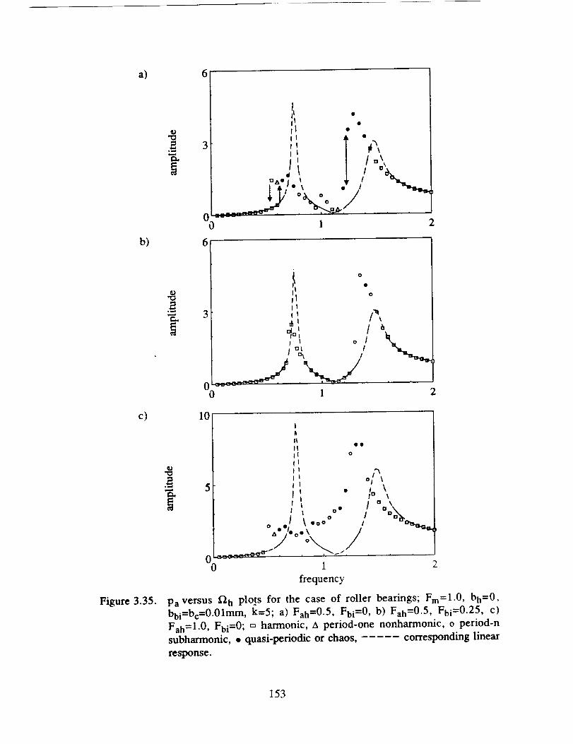
a)
b)
6
oo6
A ei B
ii J a'_II I e_,I / /,,_,'1 I J °k
.Ao/,_ ,_ / -%L/ A/ \ • I -'l'L-
J ----1 2
c)
Figure 3.35.
.2
00
10
I Oe°
It
1
I
IIIII *eII o
(I
l o/'X_
5 ; . ,,o_
/ oO- / "°2X
0 1 Z
frequency
Pa versus _h pl_s for the case of roller bearings; Fm=l.0 , bh-0 '
bbi=bc=0.01mm, k=5; a) Fah=0.5 , Fbi=0, b) Fah=0.5, Fbi=0.25, c)
Fah=l.0, Fbi=0; = harmonic, A period-one nonharmonic, o period-n
subharmonic, . quasi-periodic or chaos, " corresponding linearresponse.
153

a) 30
b)
c)
_o
20
10
!t
I!II#t
PI
IIII
0 ] 2
30
20
10
00
0
1 2
10
0o
-I C]
0
° 1
AI t • o !
_ : e_'..° o n n \A I /,, \
A / °o \_I ___ Da D
! 2
frequency
Figure 3.36. Y$ia versus flh plots for the case of deep-groove ball bearings;Fm=10 , Fah=5, Fbi=0, bh=0 , bbi=bc=0.0Olmm, a)k=l, b)k=5, c)
k=10; -, harmonic, A period-one nonharmonic, o period-n subharmonic,
• quasi-periodic or chaos, corresponding linear response.
154
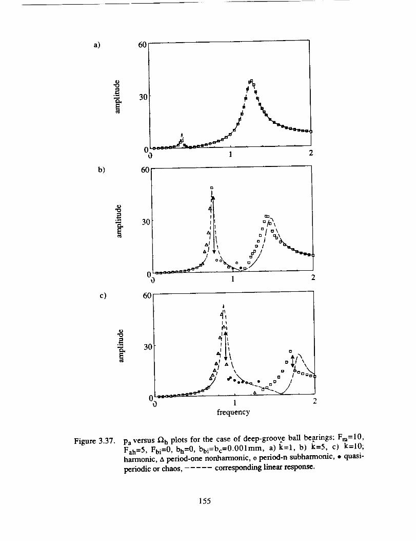
a) 60
b)
c)
!0_
0 1 2
6O
6O
_o
t_/ ch_
°_°, " ,_._-
1 2
i!
o! "_"_!_ o_;_,,,.:._. oO°°?oo_......__,_. , ,:-_.-..../, /
1 2
frequency
Figure 3.37. Pa versus _h plots for the case of deep-groove ball be_ings; Fra=lO,
Fah=5, Fbi=O, bh=O, bbi=bc=0.O01mm, a) k=l, b) k=5, c) k=lO;
harmonic, A period-one nonharmonic, o period-n subharmonic, • quasi-
periodic or chaos, • corresponding linear response.
155
validate the spur gear pair model of Chapter II assuming that the modes are weakly
coupled with each other. Now, we use the three degree of freedom non-linear model of
Figure 3.2a to analyze his test set-up [27]. In our analysis, bearings are assumed to be
linear since they were highly preloaded; only gear backlash non-linearity is considered
with 2_=0.12 mm [74]. Table 3.2 lists the system parameters used in equation (3.3a)
under four different mean loads. The system damping ratios are assumed tO be uniform
at each load. Average mesh stiffness k h and alternating load Fall values associated with
each mean load Fm are also tabulated in Table 3.2.
Figures 3.38 tl'aough 3.42 compare dynamic transmission error predictions with
the measurements [27]. At the design load (DL), which corresponds to the minimum
static transmission error, good agreement is seen except for the jump discontinuity
found experimentally at the second peak. In our model, we have increased Fah slightly
beyond the value givea in Reference [27], so that the predicted amplitude of the first
linear peak matches very well with the experiment. Such slight changes in critical
system parameters such as Fah and _, although they are varied within the experimental
uncertainties, may alter the frequency response drastically as illustrated in Figures
3.39a and 3.39b. In Figure 3.39a we note that when we reduce the force ratio Fm/Fah
from 30 (the value given in Reference [27]) to 10, a jump discontinuity at the second
peak is seen which is compatible with the experiment. Similarly, a small change in the
damping values, which are not reported in Reference [27], also affects the frequency
response as shown in Figure 3.39b. Figures 3.40 to 3.42 compare the dynamic
transmission error spectra at 3/4, 1/2 and 1/4 of the design load. From these spectra we
conclude that our proposed theory agrees well with the experimental results of Munro
[27] both qualitatively and quantitatively, although amplitudes in the off-resonance
regions are slightly off. Such amplitudes are close to the noise floor in the experiment.
156

Table 3.2. Parameters of the Munro's experimental set-up extracted from Reference
[27].
Mean load, Fm
design load(DL) 3/4 of DL 1/2 of DL 1/4 of DL
0.183 0.146 0.105 0.0579
Fah 0.0058t 0.0178 0.0296 0.0393
k b (N/m) 1.16x10⁹ 1.16x 10⁹ 1.16x10⁹ 1.16xl 09
k h (N/m) 3.44x10⁸ 3.22x10⁸ 3.01x10⁸ 2.72x10⁸
gl 1, g:22 0.950 0.966 0.983 1.007
g13, K23 0.242 0.242 0.242 0.242
_11, _22 tt 0.01 0.01 0.01 0.01
_13, _23 tt 0.00375 0.00375 0.00375 0.00375
_33tt 0.015 0.015 0.015 0.015
t modified so that the linear peak matches with the measured value.
tt estimated using the experimental data of Reference [27].
157

t_,
o
.oGO
¢J°_.._
l.O
0.5
theory
....... experiment
0.0u.4 0.8 1.2 1.6
frequency
Figure 3.38. Comparison of theory with Munro's [27] experiment at the design load.
158

a)
1..,
O
t_
4-*
u
0.4
0.2
0C-"p.4 ' 0.8 1.2 .6
b) 0.4_33--0.015
_33--0.05
!o_- . , . 1.6
frequency
Figure 3.39. Effect of a) alternating load and b) damping on the dynamic transmission
error spectrum at the design load.
159

0.8
t,_.
o
theory
....... experiment
_equency
Figure 3.40. Comparison of theory with Munro's [27] experiment at 3/4 of the design
load.
160

q)
.2
0.6
0.3
h
4°p" -_ _
theory
expem'nent
i A, ":,, :, I?,\ /':'
, i -- i-- | ,
O.8 1.2 1.6
_equency
Figure 3.41. Comparison of theory with Munro's [27] experiment at 1/2 of the design
load.
161

0
¢0
1.0
-- theory
....... experiment
frequency
Figure 3.42. Comparison of theory with Munro's [27] experiment at 1/4 of the design
load.
162

Further, discrepancies between the theory and the experiment may be due to the
assumptions made in this study. It should however be pointed out that the experiment,
even though it was very precise, was conducted almost three decades back before the
advent of modem non-linear dynamics and chaos science [66-71]. Interestingly,
Munro [27] had also reported subharmonic responses at 3/4, 1/2 and 1/4 of the design
load, and "unrepeatable responses" (probably chaos) at 1/4 of the design load. Our
results agree with such experimental observations as well. Both experiment and theory
show that the chaotic solutions dictate the frequency response beyond the second
resonance for 1/4 of the design load in Figure 3.42.
3.7. CONCLUSION
This analytical study on the non-linear dynamics of a geared rotor-bearing system
with gear backlash and bearing clearances, as excited by the intemal static transmission
error and/or external torque pulsations, has made a number of contributions to the state
of the art. First, an approximate non-linear model of the rolling element bearings with
clearances has been developed and validated. Second, our mathematical model has
been validated as it compares well with a previous experimental study, and several key
parameters such as the mean load, mean to alternating force ratio, radial bearing
preload, bearing stiffness and damping have been identified. Third, conditions for the
chaotic and subharmonic resonances, and the routes to chaos have been identified.
Forth, non-linear modal interactions have been examined. Finally, on a more
fundamental note, our study enriches the current literature on coupled vibro-impact
pairs [52,54,55].
163

CHAPTER IV
INTERACTIONS BETWEEN TIME-VARYING MESH
AND CLEARANCE NON-LINEARITIES
STIFFNESS
4.1. INTRODUCTION
Dynamic models of geared systems can be classified into four main groups. The
first group includes linear tirne-invariant (LTI) models, as evident from an extensive
review of the literature given in Reference [14]. The second group considers linear
time-varying (LTV) mesh stiffness kh(t) in the analysis [27,29,62]. Periodic variation
in kh(t) is due to the changing of the number of conjugate teeth pairs in contact during
the convolute action. Accordingly, the system is excited parametrically as well as by
the static transmission error _(_) introduced by kinematic errors and tooth deflections.
In this case, the equation of motion of the gear pair essentially reduces to the Mathieu's
or Hill's equation with a periodic external forcing function. The third group includes
gear backlash in the models, but with time-invariant average mesh stiffness k h ;e kh(i )
[25,30,31,33,34,41,42]. It should be noted that backlash is bound to exist either by
design or due to manufacturing errors and/or wear in any gear pair. Finally, the last
group considers both gear backlash and mesh stiffness variation simultaneously
[24,35-37,53]. However, none of these studies have addressed explicitly the effect of
kh(i_, including its interaction with the backlash non-linearity, on the steady state
frequency response. Ozguven and Houser [24] have attempted to analyze this problem
by replacing kh(i) with a constant mesh stiffness and by defining the "loaded static
transmission error" excitation at the mesh point. But, Ozguven [75] has stated recently
164

that this approach may not work depending on the system parameters, and
recommended a detailed investigation of this issue.
Numerous publications have analyzed LTV systems [76-78] and time-varying
systems with quadratic and/or cubic non-linearities [79-82]. However, such studies are
not directly applicable to the geared rotor systems which are the main focus of this
chapter. This problem requires the solution to a set of time-varying differential equations
with clearance-type non-linearities as excited by a periodic force generated at the gear
mesh.
4.2. PROBLEM FORMULATION
A generic geared rotor-bearing system, which consists of a spur gear pair
mounted on flexible shafts which are supported by rolling element bearings as shown
in Figure 4.1 a, is considered here. The gear box is assumed to be rigid. The effect of
the prime mover or the load inertia is not considered assuming that such inertial
elements are connected to the gear box through soft torsional couplings. Further, we
assume that the system is symmetric about the plane of the gears and the axial motion
(parallel to the shafts) is negligible. The governing equations of motion can be given in
the matrix form as
[M]{_"(t)} + [C-"]{_'(t)}+ [K(t)]{f(q(t)))= {F(t)) (4.1)
where [M] is the time-invariant mass matrix and {_(_)} is the displacement vector.
Here, damping matrix [C] is assumed to be time-invariant, as the effect of the tooth
separation and time-varying mesh properties on mesh damping are considered
negligible; validity of this assumption will be examined later. The stiffness matrix
165

rigid gear box
driving shaft
pinion
driven shaft
gear
rollingelement
bearings
(a)
Elastic
force
1 _pe stiffness
i Relative
: displacement
backlash orclearance
(b)
Figure 4.1 a) Generic geared rotor-bearing system, b) clearance non-linearity in
gears and bearings.
166

[K(i)] is considered to be a periodically time-varying matrix given by
[K(i)] =[_,(i + 2_/_h)] where _h is the fundamental gear mesh frequency. The
non-linear displacement vector {f(_(t))) includes the radial clearances in bearings and
the gear backlash as shown in Figure 4.1b, and the forcing vector {F(_)} consists of
both external torque and internal static transmission error excitations.
This chapter extends our previous non-linear single degree of freedom spur gear
pair model of Chapter 1I and multi-degree of freedom geared rotor-bearing system
model of Chapter HI by including time-varying mesh stiffness kh(i), and investigates
its effect on the frequency response of lightly and heavily loaded geared systems.
Interactions between mesh stiffness variation and system non-linearities associated with
gear backlash and radial clearances in rolling element bearings are also considered.
Resonances of the corresponding LTV system associated with the parametric and
extemal excitations are identified using the method of multiple scales. Our formulation
will be validated by comparing predictions with available experimental results [27,28].
4.3. MATHEMATICAL MODEL
A reduced order form of the multi-degree of freedom system of equation (4.1),
the three degree of freedom non-linear model of the geared rotor system, which has
been used in Chapter HI, is considered here. This includes gear inertias Ig 1 and Ig 2,
gear masses mg I and mg 2, and base circle diameters dg I and dg 2, as shown in Figure
4.2a. The gear mesh is described by a non-linear displacement function fh with time
varying stiffness kh(t) and linear viscous damping ch. Bearings and the shafts that
support the gears are modeled by equivalent elements with viscous damping
coefficients Cbl and Cb2 and non-linear springs defined by force-displacement functions
fbl _'ud fb2 which are approximated by piece-wise linear, dead zone type non-linearities
167
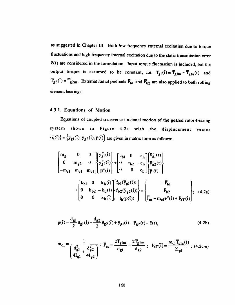
as suggested in Chapter HI. Both low frequency external excitation due to torque
fluctuations and high frequency internal excitation due to the static transmission error
_(_) are considered in the formulation. Input torque fluctuation is included, but the
output torque is assumed to be constant, i.e. Tgl(t)fTglm +Tgla(_) and
Tg2(t)-- Tg2m. External radial preloads goi and go2 are also applied to both rolling
element bearings.
4.3.1. Equalions of Motion
Equations of coupled transverse-torsional motion of the geared rotor-bearing
system shown in Figure 4.2a with the displacement vector
{_(i)} = {Ygl(i), Yg2(i), P(i)} are given in matrix form as follows:
[o" o o b, o o.lp!,<?lmg2 o/p;:<+>f+[:%:-:./L.:<,,f
L-mcl mcl mciJ{F'(i)J 0 ChJ{_(i) J
"i'L_ kb2 - kh (t)_fb2(Yg2(i))p - ' Fb2o kh6)]{ fh(_(0) J _m-mc_e"(i)+Pa'r(i)
; (4.2a)
p(i) ---dgl 0g I (i) -- dg20g 2 (i) 4-Ygl (i) -- Yg2 (i) -- ¢(i);2 2
(4.2b)
1 _ 2Tglm _ 2Tg2m= 2 - 2 ;
mcl /'dgl + dg2 i'x Fm .... dg I dg 2 , FaT(t) :
t_ _--_-,_J
m¢lTgla(i)
2Igl; (4.2c-e)
168

pinion Ogl
mg I ,I _ ,dg l//_'_
/_ gear mesh Ch
excitationS(i)rolling elementbearing modelincluding shaft
\
_;7 J gearm g2,Ig2,dg 2
(a)
pinion Og 1
I_ ,d_
gear mesh ch
excitationS(_) (
(b)
\
Figure 4.2. Non-linear models of the geared system of Figure 1; a) three degree of
freedom system, b) gear pair model with a single degree of freedom.
169

kh(t)=kh(]+_h h =khm+ = harC°S(r_ht+_hr);(4.2f)
Ygi - bbi; Ygi > bbifbi (Ygi) = 0 ; - bbi < Ygi < bbi ;
Ygi + bbi; Ygi < -bbi(_- bh); P > bh
fh(P)= 0; - bh < _ < bh. (4.2g,h)
(p + bh ); _ < -b h
Here, ( )' donates derivative with respect to time t, Ygi and 0g i are the transverse and
torsional displacements of the i-th gear (i=1,2), mcl is the equivalent gear pair mass,
Fm is the average force transmitted through the gear mesh, and FaT(t) is the fluctuating
force related to the external input torque excitation. Equations (4.2a-h) have been used
previously in Chapter HI except for k h (_) term, which is expanded in equations (4.2a-
h) in the Fourier series form. Here _(_) is the difference between the dynamic
transmission error and the static transmission error _(_). A dimensionless form of
equation (4.2a) is obtained by letting yo(t)=yo(t)/b c, p(t)=_(t)/b c,
COn= _/khm / mcl, CObi = _/kbi / mgi (i=1,2) and t = COn_ where bc is the characteristic
length. Here, we consider periodic excitation for both _(_) and FaT(t) as
¢(t)= _,erCOS(r_ht +q_er),FaT(t)= _,FaTrcos(r_Tt +q_Tr)where _h and _ arer=l r=l
the fundamental excitation frequencies of internal displacement and external torque
fluctuations, respectively. Further, define dimensionless excitation frequencies
fih =. _h/COn and fiT = fiT/COn to yield the following governing equations of
motion in the dimensionless form:
170

[oo tl[!o,31,yt,1 1.][ iS(t ) J 0 _33 Jlr,(t) J
_:11 0 Kl3(t)
+[00 K22 --K23(t)0 Kaa(t)
f, y,>lt,/t o//o tfb2(Yg2)[= Fb2 + 0 + 0 ; (4.3a)
fh(P) J [ Fm J [Fah(t)J [FaT(t)J
Fah(t) = Er=l
Cr
Fahr (rf_ h )2 cos(rflht + @er ); Fahr = bS;(4.3b,c)
FaT(t) = X FaTrCoS(rf_Tt+0Tr);r=l
FRT_FaT r = mclbctO2 ,
(4.3d,e)
gm . r_iFm_ mclbctO2 n , Fbi = mgibctO2, i=1,2;
(4.3f-g)
_ii = Cbi ; _i3 = Ch , i=1,2; _33 = Ch2mgitOn 2mgitOn 2mcle0n
(4.3hoj)
kh(t-------_) i=l,2;gii = ; gi3(t)= mgi t°2'ntDn
(4.3k-t)
K33(t) = kh(t------_)= 1 + _,8 r cos(r_ht + t_hr);khm r=l
(4.3m)
171

fb_(Yg_)=
bbi. bb__L
Ygi bc, Ygi > bc
o; - <y i <-%-.bc bc '
Ygi + bbi; ygi <-bbibc bc
fh(P) ='
bb. b_hh
P- b-_" P> bc
O" - bh < p < bh; (4.3n,o)' bc bc
P +'_c; P < b-h"bc
where Fbi (i=1,2) and F m are the dimensionless components of the mean force vector
{F}m, and FaT(t) and Fah(t) pertain to the alternating extemal excitation {F(t)}e and
internal excitation {F(t)}i force vectors, respectively.
4.4. GEAR PAIR STUDIES
First, we consider the spur gear pair model of Chapter II, as shown in Figure
4.2b, and investigate the effect of kh(i) on the steady state frequency response. The
equation of motion of the gear pair is obtained from equation (4.3a) by substituting
ygi(t)---O for fixed gear centers. Neglecting the input torque variations for the sake of
convenience, FaT(t)--0, we obtain the following equation of motion of a loaded gear
pair with time-varying mesh stiffness and backlash, as excited by the static
transmission error.
iS(t) + 2_331_(t) + g33(t)fh(p(t)) = Fm + Fah(t) (4.4)
where _33, r33 (t), fh(P), Fm and Fah are still given by equation (4.3). Since none of
the existing analytical solution methods are found to be suitable for this problem, the
digital simulation technique is used to solve equation (4.4). A 5th-6th order Runge-
Kutta numerical integration algorithm with variable time step [50] is used here. This
172

technique has already been employed successfully in Chapter II for the gear pair
problem with time-invariant mesh stiffness.
First consider only sinusoidally varying mesh stiffi_ess and the static transmission
error excitation, i.e. K33(t)-- l+ElCOS(flht+_hl) where E- _ 1 and
Fah(t) = Fahl_h 2 c°s(_ht +_el)" The tooth deflection or Fah(t) is maximum under the
applied mean load Fm when Ic33(t ) is minimum (i.e. minimum number of gear pair in
contact). Similarly, minimum Fah(t ) corresponds to maximum K33(t). Therefore, there
is an out of phase relationship between Fah(t) and g:33(t), i.e. _hl--_el+_. Here, we
set _bl=;t and d_el=0 for the sake of convenience. Hence, equation (4.4) is modified
to:
_(t)+ 2_331_(t)+ [1- Ecos(i2ht)]fh(p(t))= Fm + Fah_2 cos(I2ht). (4.5)
4.4.1. Linear Time-varying (LTV) System
For zero gear backlash bh, the gear mesh displacement function is fh(p)=p. Hence
equation (4.5) reduces to an LTV equation as follows:
_(t) + 2_331b(t) + [1 - £ cos(_ht)]p(t ) = Fm + Fah_h2 cos(flht ) (4.6)
Approximate analytical solutions of similar LTV differential equations with parametric
and external excitations are already given in the literature [76,77,79-82]. Therefore, we
wiU not attempt to solve equation (4.6) completely. Instead we identify the
corresponding resonances using the method of multiple scales [76]. A first order
uniform solution is given by an expansion having the following form where the scalar
parameter _ is assumed to be very small.
173

p(t;e) = po(To,T 1) + epl (To,T l ) + O(e 2) (4.7)
where Tn = £nt is the n-th time scale. Expansions for the derivatives with respect to t
is obtained in terms of the partial derivatives with respect to time scales D n = _ / _T n
d / dt= D O + ED l + O(E 2 ); d 2 / dt 2 = D2o + 2gDoD 1 + O(E 2 ) (4.8a,b)
Substituting equations (7) and (8) into equation (6) and equating like powers of e, with
the external force being applied at O(eO), one obtains
D2po + Po = Fin + Fahl n2 c°s(nhTo) (4.9a)
D2oPl + Pl = -2DoDIPo - I'tDoPo + Po c°s(_hTo) (4.9b)
where elx=2_33. The solution of equation (9a) is given in the complex domain as
Po = A(TI )eiT° +Fm + AeinhT° + CC; A = Fahl n2 / 2(1 - n 2 ) (4. I 0a,b)
where cc represents the complex conjugate terms and i = 4-L-i-. At fl h = 1, we note that
(1- _2)-1 will make the amplitude of the response boundless; this is the primary
resonance since it appears in the first order. Substituting equation (4.10) into equation
(4.9b) we get
174

D2pl + Pl = -2iDl AeiT° - ig .AeiT° - i_A'Oh eif_hT° + 1 Aei(l+t-lh)To2
+lAei(l_f_ h)TO+ 1 Ae2i_hTe + l Fmei[lhTo + A + cc2 2 2
(4.11)
Besides the primary resonance at fl h ---1, the particular solution of equation (4. I 1) has
other secular terms when 2fl h -- 1 and _h _ 2. At 2fl h - 1, summation of the
external excitation frequency and the parametric excitation frequency is close to the
dimensionless natural frequency which is unity. One could also observe resonances at
_'_h--n, n>2 when higher scales are considered in equation (4.7). In summary,
equation (4.6) has resonances at _h _ 0.5 and n, where n= 1,2,3 ....
Now, we solve equation (4.6) using digital simulation. Figure 4.3 shows the
steady state frequency response curves pa(flh) and pro(Oh) for a lightly loaded system
with Fro=0.1, Fahl=0.05, _33=0.05, bh=0 and four different It values. Note that E--q)
represents the LTI system. For I_>0, we do not observe any multi-valued regions and
jump phenomenon, similar to those seen for the non-linear systems. Mesh stiffness
variation E has a negligible effect on the natural frequency which corresponds to the
largest peak in Figure 4.3a; but an increase I_ in amplifies Pa in both resonance and off-
resonance regions. Here Pm is no longer uncoupled from Pa, and it varies substantially
in the vicinity of primary resonance at f_h=l.0, and the parametric resonance at
flh--0.5, especially for a large E confirming the analysis given earlier. Note that our
study is limited to only these two resonances as an investigation of subharmonic
resonances at flh _" n, n>l is beyond the scope of this study.
175

(a)
frequency
.5
Co)
0.20
0.15
0.10
frequency
Figure 4.3. Frequency response spectra of a lightly loaded LTV gear pair with
sinusoidal _(i) and kh(t), Fro=0.1 , Fahl--O.05 , _33--0.05, bh--0 and four
different e values; a)Pa versus t2h, b) Pm versus fI h.
176

4.4.2. Non.linear Time-varying System
Next we consider the time-varying non-linear system with backlash, given by
equation (4.5). Figure 4.4 shows pa(t'lh) and pm(_h) spectra with Fro--0.1, Fal=0.05,
433=0.05, and four £ values. In this case, we notice a jump discontinuity at the
resonant frequency and a dual-valued region bounded by jump-up and jump-down
transition frequencies. For £---0, Pm¢ Pm (t_h) is evident in the no-impact regime,
similar to the results given in Chapter II. But when £>0, the transition frequencies
which define the jump phenomenon become smaller, and Pa at the jump-down
frequency grows with increasing E. This indicates that kh(t) enhances the degree of
non-linearity associated with the gear backlash. Similar to the results of LTV system in
Figure 4.3, we again observe in Figure 4.4a a parametric resonance at _h---0.5, which
is strong for £=0.2 and 0.4 curves. Figure 4.5 compares the time histories p(t) for
each c values at the parametric resonance peak, _h---0.5. For the LTI system (E=0), a
harmonic no-impact type steady state solution exists as illustrated in Figure 4.5a. With
increasing E, this solution is transformed into a non-harmonic periodic solution with a
larger peak to peak value as a result of the parametric mesh stiffness excitation, as
shown in Figures 4.5b-d.
Now, consider a heavily loaded gear pair with Fro--0.1, Fal=0.01 and 433=0.05.
Figures 4.6a and 4.6b show pa(_h) and pm(_h) spectra, respectively. In this case,
tooth separation does not occur for E=0 which results in a linear frequency response
curve with a constant Pm- A small jump is seen at E---0.1, and this jump becomes larger
for £---0.2 and 0.4; overall alternating amplitudes Pa at resonance and within the off-
resonance regions increase considerably. This suggests that the mesh stiffness
variation is especially important for a heavily loaded gear pair with backlash.
177

1.0
0.5
(a)
_=0.1
.......... _---0.2
_-----0.4
0"0.0 1.2
%.
=-=.-_.=-.=--_.::=---:-_, ,0.4 0.8
_equency
o
1.2
1.0
(b)
=_----0.1
.......... _---0.2/
................ e---0.4 .,"
!,./
_ . I i I i | •O. .0 0.4 0.8 1.2
#equency
Figure 4.4. Frequency response spectra of a lightly loaded non-linear gear pair of
Figure 2bwith sinusoidal _(t) and kh(t), Fm--0.1, Fahl=0.05, _33=0.05,
bh=b c and four different _: values; a)Pa versus fl h, b) Pm versus fl h.
178
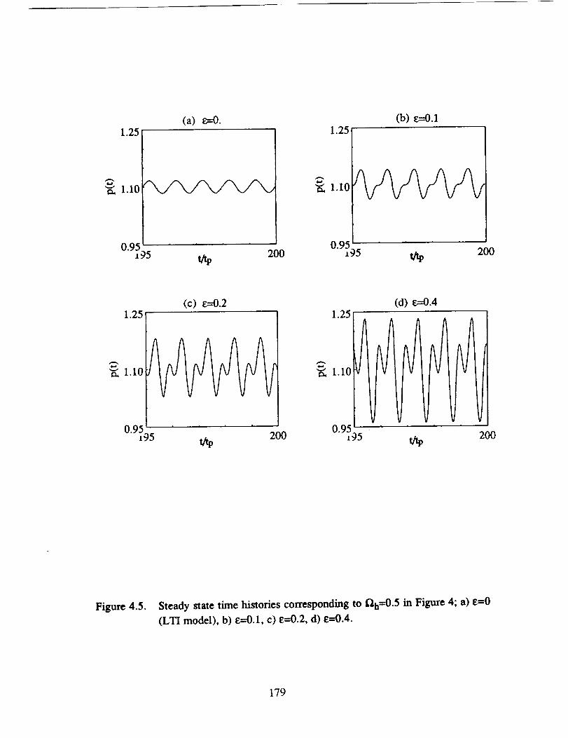
1.25
_., 1.10
(a) £=-0. (b) v_---O.11.25
i J J
0-9595 0"9595t/_ 200 _tp 200
1.25
"" 110_ •
(c) _:--'-'_.2 (d) v.,-..-0.41.25
"" 110_ •
0"9595 200 0"9595t/tp t/tp 200
Figure 4.5. Steady state time histories corresponding to _h=0.5 in Figure 4; a) e=0
(LTI model), b) I_=0.1, c) e=0.2, d) _--0.4.
179

0.6
0.3
(a)
_equency
S,3
2Ct,
1.15
1.05
(b)
...........,. -,,..,.....-,,..... - •- •--" "--"=.""--"_.?k
_-_--.-_.;_'_
f"
/- g=O.r
•" e=O.l/.-" .......... e=0.2
/" e=0.4
, i0.95u.O 0.5 1.0 1.5
_equency
Figure 4.6. Frequency response spectra of a heavily loaded non-linear gear pair with
sinusoidal _({) and kh(t), Fro=0.1 , Fahl---O.01, _33--0.05, bh=b c and four
different £ values; a)p a versus _h, b) Pm versus _h.
180

4.4.3. Non.linear Time-varying Mesh Damping
In order to investigate the effect of non-linear, time-varying gear mesh damping
on the steadystatefrequency response,we considera sinusoidallyvarying gear mesh
damping _33(t)which isassumed to be proportionalto the mesh stiffnessfunction
_33(t),and a non-linearvelocityfunctiongh associatedwith toothseparation.Hence
thegoverning equationofmotion is
j (t) + 2_33 (t)gh(15(t)) + [1 - _;cos(_ht)]fh (p(t)) = Fm + Fahf_h2 cos(_ht); (4.12a)
_33(t) = _33K33(t) = _33( 1 + Ecos(_ht + ¢_hl)) ;
0; bh bh
---<p<--gh(lb(t)) = bc bc
f)(t); else
(4.12b)
(4.12c)
Figure 4.7 compares frequency response spectra for the cases of a) non-linear time-
varying gear mesh damping defined by equation (4.12), and b) linear time-invariant
mesh damping, _33 * _33(t) with gh(15(t)) = 15(t), as given by equation (4.5). As
shown in Figure 4.7, both mesh damping models yield virtually the same spectra.
Therefore a linear time-invariant gear mesh damping model can be used without losing
any accuracy.
4.4.4. Periodic _([) and kh([)
Up to now, we have only considered the sinusodally varying kh(t) and _(t). In
real geared systems, however, both kh(t) and E(t) are periodic which can be
181

0.6
(a)
0.2
constant damping
time varying damping
0.5
! , i * ¢
1.0 1.5
frequency
(b)
1.2
1.1
1.0
---o-.-- constant damping
------- time varying damping
|i
0.5 1.0
frequency
.5
Figure 4.7. Frequency response spectra of gear pair corresponding to non-linear time
varying and line_ viscous damping models; a)Pa versus f_h, b) Pm versus
f_h.
182
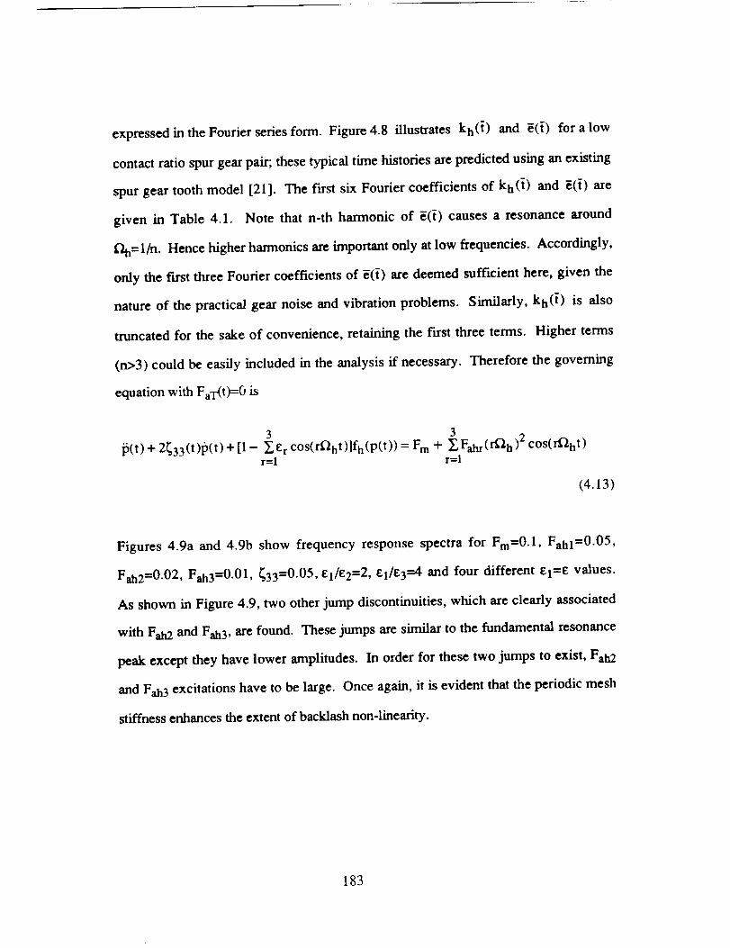
expressed in the Fourier series form. Figure 4.8 illustrates kh(t) and _(i) for a low
contact ratio spur gear pair; these typical time histories are predicted using an existing
spur gear tooth model [21]. The first six Fourier coefficients of kh(i) and _(i) are
given in Table 4.1. Note that n-th harmonic of _([) causes a resonance around
Dh=l/n. Hence higher harmonics are important only at low frequencies. Accordingly,
only the first three Fourier coefficients of [(t) are deemed sufficient here, given the
nature of the practical gear noise and vibration problems. Similarly, kh(t) is also
tnmcated for the sake of convenience, retaining the first three terms. Higher terms
(n>3) could be easily included in the analysis if necessary. Therefore the governing
equation with FaT(t)=0 is
3 3ib(t) + 2_33(t)lb(t) + [1 - EI_ r cos(rf_ht)]fh(p(t)) = Fm + _ Fahr (r_ h)2 cos(rf_ht)
r=l r=l
(4.13)
Figures 4.9a and 4.9b show frequency response spectra for Fro=0.1, Fahl=0.05,
Fah2=0.02, Fah3=0.01, 433=0.05, El/E2=2, 1;i/1;3=4 and four different I_I=E values.
As shown in Figure 4.9, two other jump discontinuities, which are clearly associated
with Fal d and Fah3, are found. These jumps are similar to the fundamental resonance
peak except they have lower amplitudes. In order for these two jumps to exist, Fah2
and Fall3 excitations have to be large. Once again, it is evident that the periodic mesh
stiffness enhances the extent of backlash non-linearity.
183

8
IJ
.*.d
Hr_
24
2O
160 ....| i
50
i
IO0
+
140
100
6O n * , m I * n * i
50 100
Figure 4.8 [(i) and kh(i) plots for a low contact ratio spur gear pair [21]. Here,
number of teeth is 28, diametral pitch is 8, the pressure angle is 20
degrees, and a 6x10 "4 in. tip modification starting at 26 degrees roll
angle is applied.
184

Table 4.1 Fourier coefficients of _(t) and kb(t) given in Figure 4.8
Harmonic n
Amplitude
kh(i)
(MN/m)
0 20.00 107.8
1 3.45 10.3
2 0.26 5.7
3 0,45 1.3
4 0.38 4.0
5 0.27 1.5
6 0.26 1.4
185

0.50
o
(a)
_'0.
_0.1
.......... e---0.2
\
0.00 .....u.O 0.4 0.8 1.2
frequency
¢:h
1.15
1.05
(b)
e--O.
e---O.1
................ c--0.2
S_ .°o-_" °'........j ,_o.B/,'/
//...."
,,/-"
.,.o
0.95 ' ,o.0 0.4 0.8 1.2
frequency
Figure 4.9. Frequency response spectra of a non-linear gear pair with periodic _(i) and
kh(t), Fro=0.1, Fahl=0.05, Fah2=0.02, Fah3-0.01 , _33=0.05, bh=bc,
C1/1_2=2, 81/_3--4 and four different glee values; a)p a versus flh, b) Pmversus _la.
186

4.5. (;EARED ROTOR.BEARING SYSTEM STUDIES
Next, we solve the three degree of freedom non-linear model of Figure 4.2a and
equation (4.3a) using the digital simulation technique for excitation Fah(t) with
FaT(t)=0.
4.5.1. Sinusoidal _([) and kh(i)
Similar to Section 4.4, assume sinusoidal forms: _33(t) = 1 + Ecos(flht + _hl )
and Fah(t)=FahlfZh2COS(f_ht+_el). Equation (4.3a) reduces to an LTV matrix
equation when gear backlash and radial bearing clearances are set to zero, i.e.
fh(P(t))--p(t) and fbi(Ygi(t))=Ygi(t), i=1,2. Figure 4.10 shows pa(flh) and Ygla(t_h)
spectra of this LTV system under heavily loaded conditions with Fro=0.1, Fahl=0.01,
_33--0.05, _i3--0,0125 and _ii=0.01, i=1, 2. Note that Ygla =Yg2a since the gear ratio
is one. As shown in Figure 4.10, frequency response has peaks at/'_h=O.)/=0.4 and
_h=03ii=1.25 where 03I and o3ii are the natural frequencies of the LTI system,
corresponding to the first two coupled transverse-torsional modes. In Figure 10a, we
observe a parametric resonance at 2f_h=O _ similar to the gear pair model of Section 4.4
whereas the parametric resonance at 2flh=031i is more obvious in pa(flh) spectrum of
Figure 4.10b for a larger e value. Again like the LTV gear pair results of Figure 4.3,
Ygla and Pa are amplified with increasing e in both resonance and off-resonance
regions.
Now introduce the gear backlash bh=b c to this heavily loaded system;
corresponding results are given in Figure 4.11. The most significant effect of kh(/) is
that it interacts with the gear backlash non-linearity to develop a jump discontinuity at
the second primary resonance peak. This is clearly evident from the fact that either
backlash or kh(i) alone can not cause a jump for such a heavily loaded system.
187
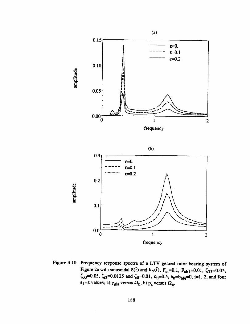
0.15
0.10
.8
0.05
0.000
(a)
t _:0.
e.---O.1
v,,-.--0.2
'i
1 2
frequency
"0
.4
0.3
0.2
0.1_
0.00
(b)
frequency
Figure 4.10. Frequency response spectra of a LTV geared rotor-bearing system of
Figure 2a with sifiusoidal _(i) and kh([) , Fm=0.1 , Fsh]=0.01 , _33=0.05,
_33=0.05, _i3--0.0125 and _ii=0.01, Kii=0.5, bh=bhbi--0 , i=l, 2, and four
el=l_ values; a) Ygia versus L'_h, b) Pa versus f_b.
188

Besides an increase in amplitudes in Figures 4.1 l a and 4.1 lb, chaotic and/or quasi-
periodic solutions, which do not exist in heavily loaded time-invariant systems as
shown in Chapter lIl, are also predicted in the following regimes: 1.35<Dh<1.65 for
£=0.2 and 1.25<t2h<l.7 for E=0.4. Similar to the LTV system of Figure 4.10,
parametric resonances at 2£_=¢o/and 2._hmgx31i are again observed here.
Next, radial clearances in bearings bbi=bc are considered for a heavily loaded
system with zero gear backlash, Fm=l.0, Fahl=0.1, _33=0.05, _i3=0.0125 and
_ii=0.01, i=l, 2. In this case, mesh stiffness variation and non-linearity exist in
different components. As shown in Figure 4.12, _ again increases the amplitudes, but
the spectrum shape is essentially the same. This is further evident from Figure 4.13,
given for a lightly loaded drive with Fm=l.0 and Fahl=0.5. This suggests a weak
interaction between the gear mesh stiffness variation and bearing non-linearities.
4.5.2. Periodic _(i) and kh(t)
Similar to the gear pair analysis of Section 4.4.4, we consider periodic g33(t) and
Fah(t) with three Fourier coefficients. Figure 4.14 shows spectra for Fro=0.1,
Fahl=0.01, Fah2=0.004, Fah3=0.002, _33=0.05, _i3=0.0125 and _ii=0.01, i=1, 2;
el/1_2=2, el/e2--4, and el=e.---O, 0.1 and 0.2. Here only the gear backlash non-linearity
(bh=b c and bbi=0) is considered. Peaks at t"lh=toi/n and £1h=e0ii/n, n=1,2,3 are
predicted corresponding to excitation Fah r. Periodic mesh stiffness enhances the
alternating amplitudes over the values given by the time-invariant mesh stiffness case
and introduces a jump discontinuity at the second primary resonance similar to the
sinusoidal mesh stiffness case.
189

0.251 _ c=O. --_
0.20; t .......... _--0.2
0.00_frequency
0.4
0.2
0.(_
(b)
E--'-O.
F._--0.1v--0.2v.---O.4
\
,\%.
•_• ° t *" °..,\ i '--.." .,.,,, / ",,.'-..:_-'_=_-
" 1
0frequency
Figure 4. I I.
geared rotor-bearing system
FrequenCy response spectra of a non-linear Fabl=O.Ol, {33=0.05,
with sinUsoidal e_) and kh(i)' Fm=O'l' bb=bc, bbi---O, i=1, 2, and
{33__.0,05' {i3_.0.0125 and {i_=0"01' _:ii=0"5'four £1=£ values; a) Ygia versus CLh,b) pa versus flh'
190
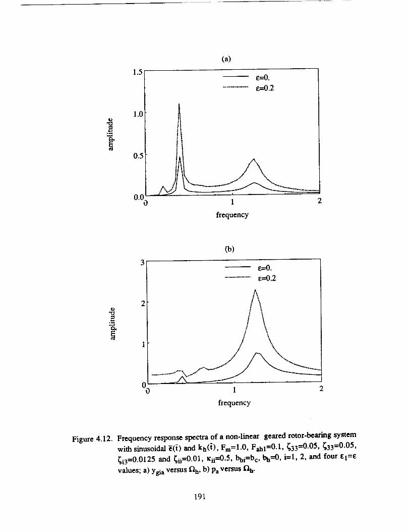
12
1.(
0.._
0.00
(a)
e--O.
............ _---0.2
flr^! ...,,il/i / \,
/j/k_ _i ° '..,,, _ -__---. .........1 2
frequency
o
3
2
00
(b)
, %
k
1 2
frequency
Figure 4.12. Frequency response spectra of a non-linear geared rotor-bearing system
with sinusoidal _(t)and kh(t), Fm=l.O, Fahl-O.1, _33=0.05, _33=0.05,
_i3=0.0125 and _ii=O.O1, tcii--0.5, bbi=bc, bh----O, i=l, 2, and four £1=E
values; a) Ygia versus f_h, b) Pa versus fl h.
191

o
2
00
!
(a)
A
i I i
1 2
frequency
o
3
00
(b)
_'0.
...... e--0.2 /\
//i\, *
"%" _,._,_ _
1 2
frequency
Figure 4.13. Frequency response spectra of a non-linear geared rotor-bearing system
with sinusoidal _(i) and kh(t), Fm-l.O, F_I--0.5 , _33--0.05, _33=0.05,
_i3=0.0125 and _ii=O.O1, Kii--0.5, bbi=bc, bh--O , i=l, 2, and four tI-E
values; a) Ygia versus _h, b) Pa versus _h.
192

o
i
0.15
0.10
(a)
e-----0.
E--0.1
_--0.2
1 2
_equency
o
.-.=
0.2i
0.1
(b)
e.---O.
e----O.1
e---0.2\
\
\
.f,,\i# ,".,/_ /, x',
- i^\ i _ f,,x\
A\17','--.9'/
I0"% 1 2
_equency
Figure 4.14. Frequency response spectra of a non-linear geared rotor-bearing system
with periodic E(i) and kb({), Fm=O.1, Fahl=0.Ol, Fab2=0.O04,
Fah3=0.002, 433=0.05, _33=0.05, _i3=0.0125 and _ii--'0.01, tcii=0.5,
bh=b¢, bbi=0, i=l, 2, £1/E2=2, El/E3---4 and three 1_1=£ values; a)Ygia
versus flh, b) Pa versus _b.
193

4.6. EXPERIMENTAL VALIDATION
4.6.|. Spur Gear Pair Dynamics
First we compare our theory with experimental results of Kubo [28], as extracted
from Reference [24]. Kubo used a heavily damped (433=0.1) four-square spur gear
test rig, and measured dynamic factor as the ratio of the dynamic to static tooth root
stresses. The experimental set-up was designed to support a gear pair with very stiff
shafts and bearings. Therefore our gear pair model can represent the test rig
adequately, similar to Chapter H. The static transmission error _([) and time-varying
mesh stiffness kh(t) of the tested gear pair has been predicted using an existing elastic
spur gear model [21] and then equation (4.4) is solved to predict the dynamic response.
Here, we define the dynamic factor as the dynamic to static mesh force ratio which is
equivalent to the dynamic factor calculation based on the stress analysis under the
assumption that the change in the moment arm due to changes in the contact point is
negligible. Figure 4.15 compares the envelope of measurements obtained by Kubo for
several tooth pairs with our predictions. When the mesh stiffness kh(t) is assumed to
be time-invadant, the predicted jump discontinuity is not as large as the jump seen in
experimental data and the predicted transition frequency is higher than the measured
value, as reported in Chapter II. However predictions improve significantly when
sinusoidally varying kh(_) and _(i) at f_h are used, as given by equation (4.5). A
sharp jump discontinuity is found which matches well with experiment, and the
predicted dynamic factor is very close to measured envelope. Finally, prediction agrees
with experiment even better when periodically varying _(-/) and kh(]-) with the first three
Fourier coefficients considered. This figure clearly shows that the time-invariant linear
or non-linear model can not predict the true dynamic behavior, as time-varying mesh
stiffness must be included in the non-linear mathematical formulation.
194

k_0
4
2
kh ;_kh(i),sinusoida] _(t)
.......... sim_soidal kh(t) and _(i)
__ periodickh(i) m_l _(t)
, , I , , I
u.2 0.6 1.0 1.4
frequency
Figure 4.15 Comparison of theory with Kubo's [24,28] experimental results.
195

4.6.2. Geared Rotor-Bearing System
As the second example case, experimental results of Munro [27] are compared
with our geared rotor-bearing model of Figure 4.2a and equation (4.3). These
experimental re.malts were used earlier to validate time-invariant multi-degree of freedom
non-linear system of Chapter rll in which we had to reduce the damping ratio and
increase the excitation [(i) in order to correlate theory with experiment. Now we go
back to the original system parameters given in References [27] and Chapter III, and
predict the dynamic transmission error spectra using both time-varying and time-
invariant gear mesh stiffness formulations for a three degree of freedom non-linear
model with gear backlash and linear bearings. Figure 4.16 compares results at the
design load which corresponds to the minimum excitation _([). In this case, the mean
load to alternating load ratio F = Fm / Fah I is very large, say F _ 30. Time-invariant
stiffness model prediction differs considerably from the experiment in Figure 4.16.
Predicted amplitudes are considerably lower than the measurements, and a significant
jump discontinuity found experimentally around the second natural frequency _ is not
even predicted by this formulation. But when the periodically-varying mesh stiffness is
considered, our model predicts the frequency response accurately including the jump
discontinuity. The reason for a large jump around ¢t)n for a very heavily loaded system
(F _ 30) is now clear. The second natural frequency _ of the corresponding LTI
system is nearly twice the first natural frequency ¢o1. This forces the second primary
resonance at _h _ ¢°I1 to coincide with the parametric resonance at f_h _ 2¢oi;
consequently a very large jump discontinuity is developed.
At 3/4 of the design load with F -- 10, the effect of kh(t) is observed in Figure
4.17. Although the time-invariant model predicts the jump at o3u, predicted amplitudes
196

i
1.0
"" experiment
time-varying mesh stiffness
time-invariant mesh stiffness
.6
frequency
Figure 4.16 Comparison of theory with Munro's [27] experiment at the design load.
197

0.9
experiment
time-varying mesh stiffness
time-invariant mesh stiffness
_l,', ,,J i i_1_/ "". ..--.,"- ',. .i/
0.8 1.2
frequency
.,,/_,,,
i
1.6
Figure 4.17 Comparison of theory with Munro's [27] experiment at 3/4 of the
design load.
198

0.8
0.4
experiment
time-varying mesh stiffness
time-invariant mesh stiffness
_...__; _l ', I ', ." "'," " k _ , I _/
0.8 1.2 1.6
frequency
Figure 4.18 Comparison of theory with Munro's [27] experiment at 112 of the
design load.
199

1.0
experiment
time-varying mesh stiffness
time-invariant mesh stiffness
frequency
Figure 4.19 Comparison of theory with Munro's [27] experiment at 1/4 of the
design load.
200

are far below the measurements. The inclusion of kh(i) improves predictions
drastically. Similarly at I/2 and 1/4 design loads, mesh stiffness variation as shown in
Figures 4.18 and 4.19 respectively, affects the frequency response significantly and
yields predictions closer to the measurements.
4.7. CONCLUDING REMARKS
This chapter on the non-linear dynamics of a geared rotor-bearing system with
time-varying mesh stiffiaess kh(t) , as excited by the static transmission error under a
mean load, has resolved a number of fundamental issues. First, the interaction between
time-varying mesh stiffness kh(t) and mean torque load has been understood.
Second, frequency response of the corresponding LTV system has been studied, and
the resonances associated with parametric and forced excitations have been identified.
Third, dynamic interactions between kh(i) and system non-linearities associated with
gear backlash and radial clearances in roiling element bearings have been investigated; a
strong interaction between kh(t) and gear backlash is found where as the coupling
between kh(t) and bearing non-linearities is weak. Finadly, our time-varying non-
linear formulation has yielded good predictions as compared with benchmark experiments.
201

CHAPTER V
CONCLUSION
5.1. SUMMARY
In this study, linear and non-linear mathematical models of a generic geared
rotor-bearing system shown in Figure I. I a are developed, and several modeling issues
which have never been addressed previously in the literature are investigated in depth.
In Chapter I, a dynamic irmite element model of the system is developed. Effects of
several system parameters such as torsional and transverse flexibilities of the shafts and
prime mover/load inertias are investigated, and modes of interest are identified. Three
reduced order linear time-invariant models are developed and the conditions under
which such models are suitable are determined by comparing the eigen-solutions with
the finite element model results.
In Chapter II, non-linear frequency response characteristics of a spur gear pair
with backlash and time-invariant mesh stiffness are examined for both external and
internal excitations. The intemal excitation is of importance from the high frequency
noise and vibration control view point and it represents the overall kinematic or static
transmission error _(t). Such problems may be significantly different from the rattle
problems associated with external, low frequency torque excitation. Two solution
methods, namely the digital simulation technique and the method of harmonic balance
have been used to develop the steady state solutions for the internal sinusoidal
excitation. Difficulties associated with the determination of the multiple solutions at a
given frequency in the digital simulation technique have been resolved as one must
202

search the entire initial conditions map. Such solutions and the transition frequencies
for various impact situations are found analytically by the method of harmonic balance.
Further, the principle of superposition can be employed to analyze the periodic
transmission error excitation and/or combined excitation problems provided the
excitation frequencies are sufficiently far apart from each other. Predictions compare
reasonably well with the experimental data available in the literature.
In Chapter 111, non-linear frequency response characteristics of a geared rotor-
bearing system are examined. A three degree of freedom dynamic model is developed
which includes non-linearities associated with radial clearances in the radial rolling
element bearings and backlash between a spur gear pair; linear time-invariant gear
meshing stiffness is assumed. Bearing non-linear stiffness function is approximated
for convenience sake by a simple model which is identical to that used for the gear
mesh. This approximate bearing model has been verified by comparing the steady state
frequency spectra. Applicability of both analytical and numerical solution techniques to
the multi-degree of freedom non-linear problem is investigated. Proposed theory is
validated by comparing the results with available experimental data. Several key issues
such as non-linear modal interactions and differences between internal static
transmission error excitation and external torque excitation are discussed. Additionally,
parametric studies are performed to understand the effect of system parameters such as
bearing stiffness to gear mesh stiffness ratio, alternating to mean force ratio and radial
bearing preload to mean force ratio on the non-linear dynamic behavior. A criterion
used to classify the steady state solutions is presented, and the conditions for chaotic,
quasi-periodic and subharmonic steady state solutions are determined. Two typical
routes to chaos observed in this geared system are also identified.
203

Non-linear frequency response characteristics of a geared rotor-bearing system
with time-varying mesh stiffness are examined in Chapter IV. The spur gear pair
model of Chapters II and geared rotor-bearing system model of Chapter 11I are
modified to include periodic mesh stiffness k h (t). Governing non-linear time-varying
equations which include clearance non-linearities associated with gear backlash and
rolling element bearings, as excited by the static transmission error _(i) under a mean
torque load, are solved using digital simulation technique. Resonances of the
corresponding linear time-varying (LTV) system associated with parametric and
external excitations are identified using the method of multiple scales and digital
simulation. Interactions between mesh stiffness variation and clearance non-linearities
have been investigated; a strong interaction between time varying mesh stiffness k h (t)
and gear backlash is found whereas the coupling between kh(t) and bearing non-
linearities is weak. The predictions yielded by the proposed time-varying non-linear
model agree well with the experimental results available in the literature.
5.2 FUTURE RESEARCH AREAS
The following topics are identified as areas of future research, based on the
present study on non-linear dynamic analysis of geared rotor-bearing systems:
1. Extension of current models to study dynamics of helical and bevel gear drives,
and multi-gear mesh systems such as planetary gear trains.
2. Iteration procedures for the transmission error input and inclusion of the
interactions between external and internal kinematic error excitations. Also
inclusion of side-bands in non-linear dynamic analysis.
204

,
.
Design of a passive vibration control strategy using squeeze Rim dampers. And,
investigation of semi-active and active vibration and noise control schemes using
piezoelectricactuatorsor hydraulicmounts.
Statisticalencrgy analysisofnon-lineargearedsystems.
205

REFERENCES
, H. D. NELSON and J. M. MCVAUGH 1976 Journal of Engineering for
Industry, American Society of Mechanical Engineers 98, 593-600. The
dynamics of rotor-bearing systems using finite elements
. E. S. ZORZI and H. D. NELSON 1977 Journal of Eng. for Power, American
Society of Mechanical Engineers 99, 71-76. Finite element simulation of rotor-
bearing systems with internal damping.
° H. D. NELSON 1980 Journal of Mechanical Design, American Society of
Mechanical Engineers 102, 793-803. A trmite rotating shaft element using
Timoshenko beam theory.
° H. N. OZGUVEN and Z. L. OZKAN 1983 American Society of Mechanical
Engineers Paper 83-DET-89. Whirl speeds and unbalance response of multi-
bearing rotors using finite elements.
. L. D. MITCHELL and D. M. MELLEN 1975 American Society of Mechanical
Engineers Paper 75-DET-75. Torsional-lateral coupling in a geared high-speed
rotor system.
° J. W. LUND 1978 Journal of Mechanical Design, American Society of
Mechanical Engineers 100, 535-538. Critical speeds, stability and response of a
geared train of rotors.
° B. M. HAMAD and A. SEIREG 1980 Journal of Engineering for Power,
American Society of Mechanical Engineers 102, 508-510. Simulation of whirl
interaction in pinion-gear systems supported on oil f'dm bearings.
206

o H. IIDA, A. TAMURA, K. KIKUCHI and H. AGATA 1980 Bulletin of
Japanese Society of Mechanical Engineers 23, 2111-2117. Coupled torsional-
flexural vibration of a shaft in a geared system of rotors (lst report).
. H. IIDA and A. TAMURA 1984 Proceedings, Conference on Vibration in
Rotating Machinery, Institution of Mechanical Engineers, 67-72. Coupled
torsional-flexural vibration of a shaft in a geared system.
10. H. IIDA, A. TAMURA and M. OONISHI 1985 Bulletin of the Japanese Society
of Mechanical Engineers 28, 2694-2698. Coupled dynamic characteristics of a
counter shaft in a gear train system.
11. H. IIDA, A. TAMURA and H. YAMAMOTO 1986 Bulletin of the Japanese
Society of Mechanical Engineers 29, 1811-1816. Dynamic characteristics of a
gear train system with softly supported shafts.
12. N. HAGIWARA, M. IDA and K. KIKUCHI 1981 Proceedings of International
Symposium of Gearing and Power Transmissions (Tokyo), 85-90. Forced
vibration of a pinion-gear system supported on journal bearings.
13. S. V. NERIYA, R. B. BHAT and T. S. SANKAR 1985 The Shock and
Vibration Bulletin 55, 13-25. Coupled torsional flexural vibration of a geared
shaft system using trmite element method.
14. H.N. OZGLrVEN and D. R. HOUSER 1988 Journal of Sound and Vibration
121,383-411. Mathematical models used in gear dynamics - a review.
15. A. KAHRAMAN, H. N. OZGUVEN, D. R. HOUSER and J. J. ZAKRAJSEK
1989 Proceedings of the ASME 5th International Power Transmission and
Gearing Conference, Chicago. Dynamic analysis of geared rotors by finite
elements.
207

16. D. DUDLEY 1984 Handbook of Practical Gear Design. New York: McGraw-
Hill.
17. D. B. WELBOURN 1979 Proceedings of the Conference on Noise and
Vibrations of Engines and Transmissions, Institution of Mechanical Engineers, 9-
14. Fundamental knowledge of gear noise-a survey.
18. D.R. HOUSER 1988 Proceedings oflnter-Noise 88 601-606. Gear noise state
of the art.
19. C. TROEDER, H. PEEKEN, A. LASCHEF and K. TOOTEN 1983 Proceedings
of International Federation of the Theory of Machines and Mechanisms Sixth
Worm Congress, New Delhi, 2, 936-943. Causes and effect of torque change in
hammering of toothed gears.
20. T. HAYASHI, N. NISHI, T. OHNO and F. R. E. CROSSLEY 1979
Proceedings of the Forth World Congress on the Theory of Machines and
Mechanisms, 350-353. Multiple impacts of a cylinder between two planes and of
a meshing teeth of a pair of gears.
21. M. S. TAVAKOLI and D. R. HOUSER 1986 Journal of mechanisms,
Transmissions and Automation in Design, Transactions of the American Society
of Mechanical Engineers 108, 86-95. Optimum profile modifications for the
minimization of static transmission errors of spur gears.
22. R.G. MUNRO 1967 The Aerospace Committee meeting of the American Gear
Manufacturers Association 1-11. Gear transmission error.
23. W. D. MARK 1987 Journal of mechanisms, Transmissions and Automation in
Design, Transactions of the American Society of Mechanical Engineers 109,
283-291. Use of the generalized transmission error in the equations of motion of
gear systems.
208
24. H, N. OZGUVEN and D. R. HOUSER 1988 Journal of Sound and Vibration
125, 71-83. Dynamic analysis of high speed gears by using loaded static
transmission error.
25. K ICHIMARU and F. HIRANO 1974 Journal of Engineering for Industry,
Transactions of the American Society of Mechanical Engineers 96, 373-381.
Dynamic behavior of heavily-load_ spur gears.
26. E.P. REMMERS 1971 American Society of Mechanical Engineers Paper 71-
DE-23. The dynamics of a gear pair system.
27. R.G. MUNRO 1962 Ph.D. Dissertation, Cambridge University. The dynamic
behaviour of spur gears.
28. A. KUBO, K. YAMADA, T. AIDA and S. SATO 1972 Transactions of Japanese
Society of Mechanical Engineers 38, 2692-2715. Research on ultra high speed
gear devices (reports 1-3).
29. K. UMF_,ZAWA, T. SATA and J. ISHIK WA 1984 Bulletin of the Japanese
Society of Mechanical Engineers 38, 102-109. Simulation of rotational vibration
of spur gears.
30. T. SAKAI, Y. DOI, K. YAMATOMO, T. OGASAWARA and M. NAR1TA
1981 SAE Paper 810773. Theoretical and experimental analysis of rattling noise
of automative gearbox.
31. S. OHNUMA, Y. SHIGETARO, I. MINEICI-II and T. FUJIMOTO 1985 SAE
Paper 850979. Research on the idling rattle of manual transmission.
32. D. C. H. YANG and J. Y. LIN 1987 Journal of mechanisms, Transmissions amt
Automation in Design, Transactions of the American Societ), of Mechanical
Engineers 109, 189-196. Hertzian damping, tooth friction and bending elasticity
in gear impact dynamics.
209

33. R.J. COMPARIN and R. SINGH 1989 Journal of Sound and Vibration 133.
Nonlinear frequency response characteristics of an impact pair.
34. R. SINGH, H. XIE and R. J. COMPARIN 1989 Journal of Sound and Vibration
130. Analysis of an automative neutral gear rattle.
35. F. KUCUKAY 1984 Proceedings of the Third Conference on Vibrations of
Rotating Machinery, Institution of Mechanical Engineers 73-79. Dynamic loads
in gear teeth.
36. R. C. AZAR and F. R. E. CROSSLEY 1977 Journal of Engineering for
Industry, Transactions of the American Society of Mechanical Engineers 99,
792-798. Digital simulation of impact phenomenon in spur gear systems.
37. K. NAKAMURA 1967 Bulletin of Japanese Society of Mechanical Engineers
10, 846-854. Tooth separation and abnormal noise on power transmission gears.
38. H. H. LIN, R. L. HUSTON and J. J. COY 1987 NASA Technical Memorandum
100180. On dynamic loads in parallel shaft transmissions, I-modeling and
analysis.
39. C.W. GEAR 1984 Computer Aided Analysis and Optimization of Mechanical
Systems, NATO ASI Series 1;'9, 323-334. Differential-algebraic equations.
40. C. W. GEAR 1984 Computer Aided Analysis and Optimization of Mechanical
Systems, NATO ASI Series F9. 335-349. The numerical solution of problems
which may have high frequency components.
41. C. C. WANG 1978 Journal of Mechanical Design, Transactions of the American
Society of Mechanical Engineers 100, 363-373. Rotational vibration with
backlash: Part 1.
210

42. C. C.WANG 1981Journal of Mechanical Design, Transactions of the American
Society of Mechanical Engineers 103, 387-397. Rotational vibration with
backlash: Part 2.
43. S.W. SHAW and P. J. HOLMES 1983 Journal of Sound and Vibration 90,
129-155. A periodically forced piecewise linear oscillator.
44. F. C. MOON and S. W. SHAW 1983 International Journal of Non-Linear
Mechanics 18, 465-477. Chaotic vibrations of a beam with non-linear boundary
conditions.
45. G.S. WHISTON 1979 Journal of Sound and Vibration 67, 179-186. Impacting
under harmonic excitation.
46. G. S. WHISTON 1987 Journal of Sound and Vibration 115, 303-319. The
vibro-impact response of a harmonically excited and preloaded one-dimensional
linear oscillator.
47. G.S. WHISTON 1987 Journal of Sound and Vibration 118, 395-429. Global
dynamics of a vibro-impacting linear oscillator.
48. Y. UEDA 1980 New Approaches to Nonlinear Problems in Dynamics. SIAM:
Philadelphia. 311-322. Steady motions exhibited by Duffmg's equation: A picture
book of regular and chaotic motion.
49. J.M.T. THOMPSON and H. B. STEWART 1986 Nonlinear Dynamics and
Chaos. John Wiley and Sons: Chichester.
50. IMSL INC. 1986 IMSL Users Manual.
51. A. GELB and W. E. VANDER VELDE 1968 Miltiple Input Describing Functions
and Nonlinear System Design. McGraw-Hill: New York.
211

52. L. E. GALHOUD, S. F. MASRI and J. C. ANDERSON 1987 Journal of
Applied Mechanics, Transactions of the American Society of Mechanical
Engineers 54, 215-225. Transfer function of a class of nonlinear multidegree of
freedom oscillators.
53. H. WINTER and M. KOJIMA 1981 Proceedings of the Intemational Symposium
on Gearing & Power Transmissions, Tokyo c-12. A study on the dynamics of
geared system - estimation of overload on gears in system.
54. R. J, COMPARIN and R. SINGH 1989 Submitted to Journal of Sound and
Vibration. Frequency response characteristics of coupled impact pairs,
55. R. J. COMPARIN and R. SINGH 1989 Journal of Mechanical Design,
Transactions of the American Society of Mechanical Engineers (in press). An
analytical study of automotive neutral gear rattle.
56. A. H. NAYFEH 1983 Journal of Sound and Vibration 90, 237-244. The
response of multidegree-of-freedom systems with quadratic non-linearities to a
harmonic parametric resonance.
57. A. G. HADDOW, A. D. S. BARR and D. T. MOOK 1984 Journal of Sound and
Vibration 97, 451-473. Theoretical and experimental study of modal interaction
in a two-degree-of freedom structure.
58. D. T. MOOK, R. H. PLAUT and N. HAQUANG 1985 Journal of Sound and
Vibration 102,473-492. The influence of an internal resonance on non-linear
structural vibrations under subharmonic resonance conditions.
59. D. T. MOOK, N. HAQUANG and R. H. PLAUT 1986 Journal of Sound and
Vibration 104, 229-241. The influence of an internal resonance on non-linear
structural vibrations under combined resonance conditions.
212

60.
61.
M. P. CARTMELL and L W. ROBERTS 1988 Journal of Sound and Vibration
123, 81-101. Simultaneous combination resonances in an autoparametric
resonant system.
D. A. STREIT, A. K. BAJAJ and C. M. KROUSGRILL 1988 Journal of
Sound and Vibration 124, 297-314. Combination parametric resonance leading
to periodic and chaotic response in two-degree-of freedom systems with quadratic
non-linearities.
62.
63.
M. HORTEL 1967 Proceedings of the Fourth Conference on Non-linear
Oscillations, 337-346. Forced damped vibrations in a nonlinear parametric
system of gears with several degrees of freedom.
T. A. HARRIS 1966 Rolling Bearing Analysis. John Wiley and Sons: New
York.
64.
65.
M. F. WHITE 1979 Journal of Applied Mechanics, Transactions of the
American Society of Mechanical Engineers 46, 677-684. Rolling element
bearing vibration transfer characteristics: effect of stiffness.
T. C. LIM and R. SINGH 1989 Submitted to Journal of Sound and Vibration.
Vibration transmission through rolling element bearings, part I: bearing stiffness
formulation.
66. F.C. MOON 1987 Chaotic Vibrations. John Wiley & Sons: New York.
67.
68.
C. GREBOGI, E. OT'I', S. PELIKAN and J. A. YORKE 1984 Physica 13D,
261-268. Strange attractors that are not chaotic.
J. M. T. THOMPSON and H. B. STEWART 1986 Nonlinear Dynamics and
Chaos. John Wiley and Sons: Chichester.
213

69. J.D. CRAWFORD and S. OMOHUNDRO 1984 Physica 13D, 161-180. On the
global structure of period doubling flows.
70. J.B. MCLAUGHLIN 1981 Journal of Statistical Physics 24, 375-388. Period-
doubling bifurcations and chaotic motion for a parametrically forced pendulum.
71. H.G. SCHUSTER 1984 Deterministic Chaos. Physik-Vedag: Weinheim.
72. A. KUBO 1989 Private communication.
73. J. KRAUS, J. J. BLECH and S. G. BRAUN 1987 Journal of Vibration,
Acoustics, Stress, and Reliability in Design, Transactions of the American
Society of Mechanical Engineers 109, 235-240. In situ determination of rolling
bearing stiffness and damping by modal analysis.
74. R.G. MUNRO 1989 Private communication.
75. H.N. OZGUVEN 1989 Research Report, the Ohio State University, Columbus,
Ohio.
76. A. H. NAYFEH and D. T. MOOK 1979 Nonlinear Oscillations. Wiley-
Interscience: New York.
77. A.H. NAYFEH 1985 Problems in Perturbation.Wiley-Interscience: New York.
78. J. A. RICHARDS 1983 Analysis of Periodically Time-Varying Systems.
Spdnger-Veflag: New York.
79. H. TROGER and C. S. HSU 1977 Journal of Applied Mechanics, Transactions
of the American Society of Mechanical Engineers 44, 179-181. Response of a
nonlinear system under combined parametric and forcing excitation.
80. C. S. HSU and W. H. CHENG 1974 Journal of Applied Mechanics,
Transactions of the American Society of Mechanical Engineers 41, 371-378.
214

Steady state response of a dynamical system under combined parametric and
forcing excitation.
81. N. HAQUANG, D. T. MOOK and R. H. PLAUT 1987 Journal of Sound and
Vibrations 118, 425-439. A non-linear analysis of the interactions between
parametric and external excitations.
82. N. HAQUANG 1986 Ph.D. Thesis, Virginia Polytechnic hlstitute and State
University. Response of non-linear structural systems to multifrequency
excitations.
215
APPENDIX A
USER'S GUIDE FOR THE GEARED ROTOR DYNAMICS
PROGRAM - GRD
A.I. DESCRIPTION
Geared Rotor Dynamics Program "GRD" is a general purpose f'mite element
computer program to analyze dynamics of a system consisting of two shafts supported
on bearings and coupled by a gear mesh. It computes natural frequencies, mode shapes
and the vibration response of the system to static transmission error excitation, mass
unbalances and geometric eccentricities of gears. Many rigid disks, bearings, and
hollow shafts can be considered by GRD. Since GRD uses finite elements method, the
system should first be discretized to small rotor elements. It is also necessary to enter
data for each element in sequence.
A.2. USING THE PROGRAM
There are two ways to input data in GRD. Data can be entered through a file or
interactively. The first set of questions will give the user this option (the Primary
t_Q_j_). Display on screen:
ENTER DATA INTERACTIVELY OR FROM A DATA FILE7OPTION (1) : ENTER DATA INTERACTIVELYOPTION (2) : ENTER DATA FROM FILE
CHOOSE OPTION I OR 2 (NO DEFAULT) >> b
A.2.1. OPTION I: Interactive Data Entry
By selecting this option, the user will be prompted to enter all the data that will be
necessary to run this program. In the process, a new data f'de will be created from the
user's input. The data entered will be reorganized in a format so that the program may
read from it. For this reason, a new data file will be created and the user will be
prompted to name this new fde as follows:
DATA WILL BE INPUT INTERACTIVELY, AND IN THE PROCESS, YOUR INPUTWILL BE ORGANIZED'IN A NEW DATA FILE FOR THIS PROGRAM TOREAD FROM.
ENTER AN INPUT FILE NAME >> __
216

If an error should arise from opening this new file, the user will be given the option to
try gain:
*ERROR IN OPENING FILE* DO YOU WISH TO TRY AGAIN?
TYPE (1) FOR YES OR (2) FOR NO >>__
If YES, then the user will be asked the file name again. If NO, the program will
return to the Primary Option.
2.1.1. Data Entry Groupings
In this section, the user will enter the necessary data. The questions will be
grouped into the following categories.
1. GENERAL DATA2. MATERIAL PROPERTIES3. ELEMENT PROPERTIES4. GEAR MESH PROPERTIES
5. FORCED RESPONSE DATA (If user chooses this option)
1. _;¢n¢ral Data:
In this section, the following general information about the overall system will be
entered:
I) THE NUMBER OF ROTOR ELEMENTS IN THE FIRST SHAFT2) THE NUMBER OF ROTOR ELEMENTS IN THE SECOND SHAFT3) THE NUMBER OF ROTOR ELEMENTS BEFORE THE GEAR IN THE FIRST SHAFT4) THE NUMBER OF ROTOR ELEMENTS BEFORE THE GEAR IN THE SECOND
SRAFF
As an example, consider the system shown in Figure AI. The fast step is to the
divide rotors into small pieces (irmite rotor elements) to obtain a finite dement model of
the system (as illustrated in Figure A2). The shorter the rotor elements, the higher the
accuracy and the longer the computation time. In Figure A2, each shaft is divided into
4 pieces. The numbering can start at any end of the driving rotor and finish at any end
217

PINION
FIRST SHAFT
COND SHAFT m
ww
w
mwu
Figure A1. A Typical Geared Rotor System
BEARING
I
®
I{ I1 2
ROTORELEMENT
J! "+ I
®
GEAR 1
1_3 (Pn_TI°N)II
4
I I I!7
GEAR 2
(GEAR)
8
!
I
®
Figure A2. Finite Element Model
218

of the driven rotor. In Figure A2 for example, we start at the left end of the first shaft
and finished numbering at the right end of the second shaft. According to this
configuration (Figure A2), the number of rotor elements in the first and second shafts
are both 4 and the number of rotor elements before the pinion and gear axe 2 and 6,
respectively.
2. Material Properties:
In this section, material properties of the shaft considered will be entered. The
following will be required:
1 ) THE DENSITY OF THE SHAFT MATERIAL (kg/m 3)
2) THE VISCOUS DAMPING COEFFICIENT (s)3) THE HYSTERETIC DAMPING COEFFICIENT
4) THE MODULUS OF ELASTICITY (N/m 2)
5) SHEAR MODULUS OF ELASTICITY (N/m 2)
(DE.FAULT=7800)
(DEF--0)
(DEF---0)
(DEF=.207EI2)
(DEF=.0795EI2)
3. Element ProDertie_;
The main portion of data to be entered is in this section. The options given are the
foUowing:
1) DEFINING THE DISK ELEMENT2) DEFINING THE BEARING ELEMENT3) DEFINING THE ROTOR ELEMENT (also the default selection)4) DEFINING THE GEAR ELEMENT5) FINISH WITH DATA INPUT FOR FIRST SHAFT6) FINISH WITH DATA INPUT FOR SECOND SHAFT
The most important part in this section of questions is the order of data entry. The
order is based on the numbered finite element model (see Figure A2). For the lrmite
element model shown in Figure A2, the order of data input is as follows:
1) DEFINING BEARING #12) DEFINING ROTOR #13) DEFINING ROTOR #'24) DEFINING GEAR#15) DEFINING ROTOR #36) DEFINING ROTOR #-47) DEFINING BEARING #28) TYPE IN OPTION 5 (FINISHED WITH DATA INPUT FOR SHAFT #I)9) DEFINING BEARING #310) DEFINING ROTOR #511) DEFINING ROTOR #6
219

12) DEFINING GEAR#213) DEFINING ROTOR #714) DEFINING ROTOR #815) DEFINING BEARING #416) TYPE IN OPTION 6 (FINISHED WITH DATA INPUT FOR SHAFT #2)
From the example above, one can see the ordering of data entry moving from the first
element in shaft #1 to the last element in shaft #2. Ultimately, the program will also
read from the data file in this order.
According to the option selected (disk, gear, rotor element or bearing), the
following information is required:
The disk element - option 1:
1) DISK OUTER DIAMETER IN (m)2) WIDTH OR THICKNESS OF DISK IN (m)
3) MATERIAL DENSITY OF DISK IN (kg/m 3) (DEF=7800)
The bearing element - option 2:
THE ST_'FN_S (N/m)I)Kxx
2)Kxy
3)Kyx
4)KyyTHE DAMPING (N-slm_
5) Cxx
6) Cxy
7) Cyx
8) Cyy
The rotor dement - option 3:
1) LENGHT OF ROTOR ELEMENT IN (m)2) OUTER DIAMETER OF ROTOR ELEMENT IN (m)
3) INNER DIAMETER OF ROTOR ELEMENT IN (m) (for hollow rotor) (DEF=0)4) THE AXIAL LOAD IN (N) (DEF_0)
The gear dement - option 4:
1) PITCH CIRCLE DIAMETER IN (m)2) FACE WIDTH IN (m)
220

3) GEAR MATERIAL DENSITY IN (kg/m 3) (DEF=T800)
Option 5 should be chosen when the elements of the first shaft have been defined.
The user will then be given the material properties of the second shaft., and given the
option to make changes to this set of data. Similarly, option 6 should be entered
when all elements of the second shaft have been entered.
4, Q¢_r Mesh Properties:
The following gear mesh properties will be entered in this section:
1) GEAR MESH STIFFN_S (N/m)2) GEAR MESH DAMPING (N-s/m)3) BASE CIRCLE DIAMETER OF FIRST GEAR (m)4) BASE CIRCLE DIAMETER OF SECOND GEAR (m)
fDEF=0)
Following the input of gear mesh data, the program will also ask the user for the
number of natural frequencies wanted in the output.
$. Forced Response Data:
Here, the user is given the option to have forced response calculated. If the
selection is NO, then interactive input will be complete. If the selection is YES, then
the following options are given:
1) WHIRLING ORBIT AT A SPECIFIED NODE2) DEFLECTIONS AT A SPECIFIED NODE3) DYNAMIC LOAD TO STATIC LOAD RATIO AT THE MESHING POINT
Following the options menu, the general information for this section will be required:
1) GEOMETRIC ECCENTRICITY (RUNOUT) OF GEAR 1 (m)2) GEOMETRIC ECCENTRICITY (RUNOUT) OF GEAR 2 (m)3) PEAK TO PEAK VALUE OF STATIC TRANSMISSION ERROR (m)4) MASS UNBALANCE OF GEAR 1 (kg-m)5) MASS UNBALANCE OF GEAR 2 (kg-m)6) NUMBER OF TEETH IN GEAR 1 (PINION)7) AVERAGE FORCE TRANSMITIED (hi)8) VALUE OF MODAL DAMPING
(DEF=0)(DEF_0)
(DEF=O)(DEF=0)
(DEF=.01)
After the general information for this section has been completed, the program will
require certain information based from the choice selected from the options menu :
221

Forced response option 1: Whirling orbit at a specified node, the following
information will be required.
1) NUMBER OF NODE AT WHICH WHIRL ORBIT IS REQUIRED2) ROTATIONAL SPEED OF SHAFT I (tad/s)
Forced response option 2: Deflections at a specified node will be required.
1) STARTING ROTATIONAL SPEED OF SHAFT 1 (tad/s) (DEF=0)2) UPPER LIMIT OF ROTATIONAL SPEED OF SHAFT I (tad/s)3) INCREMENT FOR ROTATIONAL SPEED (tad/s) (DEF=5)4) DIRECTION AT WHICH FORCED RESPONSE IS WANTED (1,2 OR 3) (DEF=I)5) NUMBER OF NODE AT WH1CH FORCED RESPONSE IS WANTED
In question (4), enter: 1 for deflection in pressure line direction; 2 for deflection in
direction perpendicular to pressure line; 3 for torsional deflections
1) STARTING ROTATIONAL SPEED OF SHAFT 1 (tad/s)2) UPPER LIMIT OF ROTATIONAL SPEED OF SHAFT 1 (rad/s)3) INCREMENT FOR ROTATIONAL SPEED (tad/s)
(DEF=0)
(DEF=5)
Having completed this section on forced response, the program will then read from the
new data file created from the interactive input. The output will be in an output data file
named FOR001.DAT .
A.2.2. OPTION 11: Enter Data From File
With this selection, the user is then requested to give the name of the file where the
data is stored, instead of entering data interactively. The program will then proceed to
read from the file. If an error should occur in opening the trde, then the user will be
given the option to try again. If the user opts to try again, then the user will be asked
the file name again. If no, then the program will return to the primary option. After the
program has read from the file the output will be found in an output data f'de.
222

A.4. SAMPLE OUTPUT FILE FOR001.DAT
GEARED ROTOR DYNAMICS PROGRAM
GILD
GEAR DYNAMICS AND GEAR NOISE RESEARCH LABORATORY
THE OHIO STATE UNIVERSITY
THE FIRST SHAFT:
MATERIAL PROPERTIES OF THE SHAFT:
DENSITY OF THE MATERIAL ..... =
ELASTIC MODULUS ............. =
SHEAR MODULUS ............... =
VISCOUS DAMPING COEFFICIENT.=
HYSTERETIC LOSS FACTOR ...... =
0.78000E+04 KG/M**3
0.20700E+12 N/M**2
0.79500E+11 N/M**2
0.00000E+00 S
0.00000E+00
AT Z- 0.0000 M THERE EXISTS A BEARING WITH THE
FOLLOWING STIFFNESS AND DAMPING COEFFICIENTS:
KXX= 0.10000E+I0 N/M KXY--
KYX= O.O0000E+O0 N/M _=
CXX- 0.00000E+00 N-S/M CXY-
CYX= 0.00000E+00 N-S/M CYY =
0.00000E+00 N/M
0.10000E+I0 N/M
0.00000E+00 N-S/M
0.00000E+00 N-S/M
AT Z- 0.0000 M THERE EXISTS A FINITE ROTOR ELEMENT WITH THE
FOLLOWING SPECIFICATIONS:
LENGTH OF THE ELEMENT ....... -=
OUTER DIAMETER .............. -=
INNER DIAMETER .............. ,-
AXIAL LOAD .................. -,
0.50000E-01 M
0.30000E-01 M
0.00000E+00 M
0.00000E+00 N
AT Z-- 0.0500 M THERE EXISTS A FINITE ROTOR ELEMENT WITH THE
FOLLOWING SPECIFICATIONS:
LENGTH OF THE ELEMENT .......
OUTER DIAMETER ..............
INNER DIAMETER .............. --
AXIAL LOAD .................. -
0.50000E-01 M
0.30000E-01 M
0.00000E+00 M
0.00000Z+00 N
AT Z- 0.i000 M THERE EXISTS A RIGID DISK WITH THE FOLLOWING
SPECIFICATIONS:
OUTER DIAMETER ...... = 0.13500E+00 M
223

WIDTH ............... -"
MATERIAL DENSITY .... -_
0.25400E-01 M
0.78000E+04 KG/M**3
AT Z- 0.I000 M THERE EXISTS A FINITE ROTOR ELEMENT WITH THE
FOLLOWING SPECIFICATIONS:
LENGTH OF THE ELEMENT ....... --
OUTER DIAMETER .............. --
INNER DIAMETER .............. --
AXIAL LOAD .................. -
0.50000E-01 M
0.30000E-01 M
0.00000E+00 M
0.00000Z+00 N
AT Z-- 0.1500 M THERE EXISTS A FINITE ROTOR ELEMENT WITH THE
FOLLOWING SPECIFICATIONS:
LENGTH OF THE ELEMENT .......
OUTER DIAMETER .............. =
INNER DIAMETER .............. =
AXIAL LOAD .................. =
0.50000E-01 M
0.30000E-01 M
0.00000E+00 M
0.00000Z+00 N
AT Z= 0.2000 M THERE EXISTS A BEARING WITH THE
FOLLOWING STIFFNESS AND DAMPING COEFFICIENTS:
KXX- 0.10000E+I0 N/M KXY--
KYX-- 0.00000E+00 N/M KYY-
CXX_ 0.00000E+00 N-S/M CXY-
CYX- 0.00000E+00 N-S/M CYY-
0.00000E+00 N/M
0.10000E+10 N/M
0.00000E+00 N-S/M
0.00000E+00 N-S/M
THE SECOND SHAFT:
MATERIAL PROPERTIES OF THE SHAFT:
DENSITY OF THE MATERIAL ..... =
ELASTIC MODULUS ............. =
SHEAR MODULUS ............... -
VISCOUS DAMPING COEFFICIENT.=
HYSTERETIC LOSS FACTOR ...... -
0.78000E+04 KG/M**3
0.20700E+12 N/M**2
0.79500E+11 N/M**2
0.00000E+00 S
0.00000E+00
AT Z- 0.0000 M THERE EXISTS A BEARING WITH THE
FOLLOWING STIFFNESS AND DAMPING COEFFICIENTS:
KXX- 0.10000E+Z0 N/M KXY-
KYX- 0.00000E+00 N/M KYY-
CXX- 0.00000E+00 N-S/M CXY-
CYX- 0.00000E+00 N-S/M CYY-
0.00000E+00 N/M
0.10000E+10 N/M
0.00000Z+00 N-S/M
0.00000E+00 N-S/M
AT Z- 0.0000 M THERE EXISTS A FINITE ROTOR ELEMENT WITH THE
FOLLOWING SPECIFICATIONS:
LENGTH OF THE ELEMENT ....... =
OUTER DIAMETER .............. --
INNER DIAMETER .............. -
AXIAL LOAD .................. -
0.50000E-01M
0.40000E-01 M
0.00000Z+00 M
0.00000E+00 N
224

AT Z= 0.0500 M THERE EXISTS A FINITE ROTOR ELEMENT WITH THE
FOLLOWING SPECIFICATIONS:
LENGTH OF THE ELEMENT ....... =
OUTER DIAMETER .............. --
INNER DIAMETER .............. t
AXIAL LOAD .................. -
0.50000E-01 M
0.40000E-01 M
0.00000Z+00 M
0.00000Z+00 N
AT Z- 0.1000 M THERE EXISTS A RIGID DISK WITH THE FOLLOWING
SPECIFICATIONS:
OUTER DIAMETER ...... -
WIDTH ............... --
MATERIAL DENSITY .... -
0.24500E+00 M
0.25400E-01 M
0.78000E+04 KG/M**3
AT Z- 0.1000 M THERE EXISTS A FINITE ROTOR ELEMENT WITH THE
FOLLOWING SPECIFICATIONS:
LENGTH OF THE ELEMENT ....... --
OUTER DIAMETER .............. u
INNER DIAMETER .............. -
AXIAL LOAD .................. =
0.50000E-01 M
0.40000E-01 M
0.00000E+00 M
0.00000E+00 N
AT Z- 0.1500 M THERE EXISTS A FINITE ROTOR ELEMENT WITH THE
FOLLOWING SPECIFICATIONS:
LENGTH OF THE ELEMENT ....... =
OUTER DIAMETER .............. -
INNER DIAMETER .............. -
AXIAL LOAD .................. -
0.50000E-01 M
0.40000E-01 M
0.00000E+00 M
0.00000E+00 N
AT Z- 0.2000 M THERE EXISTS A BEARING WITH THE
FOLLOWING STIFFNESS AND DAMPING COEFFICIENTS:
KXX-- 0.10000E+10 N/M KXY=
KYX= 0.00000E+00 N/M KYY-
CXX- 0.00000E+00 N-S/M CXY-
CYX- 0.00000E+00 N-S/M CYY-
0.00000E+00 N/M
0.10000E+I0 N/M
0.00000E+00 N-S/M
0.00000E+00 N-S/M
GEAR MESH PROPERTIES:
BASE CIRCLE DIAMETER OF GEAR 1...-
BASE CIRCLE DIAMETER OF GEAR 2...-
AVERAGE MESH STIFFNESS ........... =
AVERAGE MESH DAMPING ............. --
0.1270 M
0.2310 M
0.20000E+09 N/M
0.00000E+00 N-S/M
A. FREE VIBRATION ANALYSIS:
FOLLOWING NATURAL FREQUENCIES AND MODESHAPES ARE CALCULATED
FOR THE ABOVE SPECIFIED SYSTEM:
225

MODE 1
NATURAL FREQUENCY- 0.0002 (BZ.)
CORRESPONDING MODESHAPES:
DISP. IN Y DISP. IN X ROT. ABOUT Y ROT. ABOUT X ROT. ABOUT Z
-.260E-08 0.000E+00 0.000E+00 -.105E-06 0.599E+01
-.358E-08 0.000E+00 0.000E+00 0.108E-06 0.599E+01
0.119E-08 0.000E+00 0.000E+00 -.411E-07 0.599E+01
-.524E-08 0.000E+00 0.000E+00 -.983E-07 0.599E+01
-.299E-08 0.000E+00 0.000E+00 0.136E-06 0.599E+01
0.771E-08 0.000E+00 0.000E+00 0.499E-06 0.329E+01
0.253E-07 0.000E+00 0.000E+00 0.535E-07 0.329E+01
-.188E-09 0.000E+00 0.000E+00 -.118E-05 0.329E+01
-.256E-07 0.000E+00 0.000E+00 0.557E-07 0.329E+01
-.781E-08 0.000E+00 0.000E+00 0.505E-06 0.329E+01
MODE 2
NATURAL FREQUENCY= 486.0262 (HZ.)
CORRESPONDING MODESHAPES:
DISP. IN Y DISP. IN X ROT. ABOUT Y ROT. ABOUT X ROT. ABOUT Z
0.929E-02 0.000Z+00
0.261E+00 0.000E+00
0.375E+00 0.000E+00
0.261E+00 0.000E+00
0.929E-02 0.000E+00
-.950E-02 0.000E+00
-.918E-01 0.000E+00
-.129E+00 0.000E+00
-.918E-01 0.000E+00
-.950E-02 0.000E+00
0 000E+00
0 000E+00
0 000E+00
0 000E+00
0 000E+00
0 000E+00
O.O00E+O0
0.000E+00
0.000E+00
0.000Z+00
0.551E+01 -.646E+01
0.410E+01 -.645E+01
-.I19E-06 -.643E+01
-.410E+01 -.645E+01
-.551E+01 -.646E+01
-.180E+01 0.110E+01
-.134E+01 0.110E+01
0.995E-09 0.109E+01
0.134E+01 0.110E+01
0.180E+01 0.110E+01
226

MODE I0
NATURAL FREQUENCY= 2479.9504 (HZ.)
CORRESPONDING MODESHAPES:
DISP. IN Y DISP. IN X ROT. ABOUT Y ROT. ABOUT X ROT. ABOUT Z
0.124E-01 0.000E+00 0.000E+00 0.459E+01 0.978E+01
0.212E+00 0.000E+00 0.000E+00 0.288E+01 0.950E+01
0.279E+00 0.000E+00 0.000E+00 -.897E-10 0.865E+01
0.212E+00 0.000E+00 0.000E+00 -.288E+01 0.950E+01
0.124E-01 0.000E+00 0.000E+00 -.459E+01 0.978E+01
-.990E-02 0.000E+00 0.000E+00 -.134E+01 -.166E+01
-.691E-01 0.000E+00 0.000E+00 -.897E+00 -.162E+01
-.917E-01 0.000E+00 0.000E+00 -.562E-10 -.147E+01
-.691E-01 0.000E+00 0.000E+00 0.897E+00 -.162E+01
-.990E-02 0.000E+00 0.000Z+00 0.134E+01 -.166E+01
B. FORCED VIBRATION ANALYSIS:
FORCED RESPONSE AT THE
0.591142E-04
0.675386E-04
SPECIFIED FREQUENCY RANGE:
227

APPENDIX B
DIMENSIONAL AND NON-DIMENSIONAL QUANTITIES
FOR THE EXPERIMENTAL TEST RIGS
Table BI. Dimensionless and dimensional parameters for Kubo's test rig [28].
DIMENSIONAL QUANTITIES
Number of teeth
Igl, Ig2 [kg-m 2 (Ib-ft2)]
rnc_ lkg]
dgl, dg 2 [m (in)]
kbk h [N/m 0bf/'m)]
Fm IN (lbf)]
[m (in)]
[m (in)]
25/25
0.00115 (0.0278)
0.23
0.094 (3.7)
rigid3.8E8 (2.17E6)
2295 (1030)
1.92E-6 (7.56E-5)
0. IE-3 (0.0039)
DIMENSIONLESS QUAN'Ilq]_
(page ,14)
Fm (page 44)
Fah (page 44)
Fm/F_
0.1
0.06
0.0192
3.12
228

Table B2. Dimensionless and dimensional parameters for Munro's test rig [27].
DIMENSIONAL QUANTITIES
number of tveth 32/32
Isl, Ig 2 [kg-m 2 (lb-ft2)] 0.136 (3.29)
ms], ms2 [kg (lb)] 31.1 (68.5)
dg l, dg 2 [m (in)] 0.2 (8)
bh [m (in)] 0.12E-3 (4.7E-3)
Design Load (DL) 3/4 DL 1/2 DL 1/4DL
Fm [N (lbf/in FW)] 3782 (1700) 2836 (1275) 1891 (850) 947 (425)
k h [N/m ] 3.44E8 3.22E8 3.01E8 2.72E8
% [In] 3.5E-7 1.06E-6 1.78E-6 2.36E-6
DIMENSIONLESS QUANTFFIES
Design Load (DL) 3/4 DL 1/2 DL 1/4 DL
Fm (equation 3.3i) 0.183 0.146 0.105 0.058
Fah (equation 3.3j) 0.0058 0.0178 0.0296 0.0393
K:11,1¢22 (equation 3.3f) 0.950 0.966 0.983 1.007
K:I3, K:23 (equation 3.3g) 0.242 0.242 0.242 0.242
_11, _22 (equation 3.3c) 0.01 0.01 0.01 0.01
_13, _23 (equation 3.3d) 0.00375 0.00375 0.00375 0.00375
_33 (equation 3.3e) 0.015 0.015 0.015 0.015
229

APPENDIX C
LENGTH OF TRANSIENT SOLUTION AND CPU TIME
C.I. Length of Transient Solution
It is necessary to run the digital simulation routines for many cycles in order to
reach the steady state solution. This can easily be detected by a time history repeating
itself and a phase plane trajectory followed at each period of the steady state solution.
Following are found to be the major factors which determine the length of the transient
region of the time history:
1. Damping Ratio; Damping ratio is inversely proportional to the time needed to
reach steady state solution. Larger the damping, shorter the transients. Figure B I
shows this relationship for the single degree of freedom model of gear pair. A similar
trend is observed in Multi-degree of freedom model also.
2. Excitation Frequency; The transient solution is found to be longer in the
vicinity of the resonance frequency than the off-resonance region. Figure B 1 compares
length of transient solution versus damping ratio curves corresponding to resonance
and off-resonance excitation frequencies.
3. Initial Conditions; Transients are longer when the initial displacement and
velocity are away from the mean values of the steady state solution sought.
C.2. CPU Times
CPU time needed in digital simulation depends on: i. the number of increments
per period of forcing function (20-40 points per period is good enough), ii. the
230
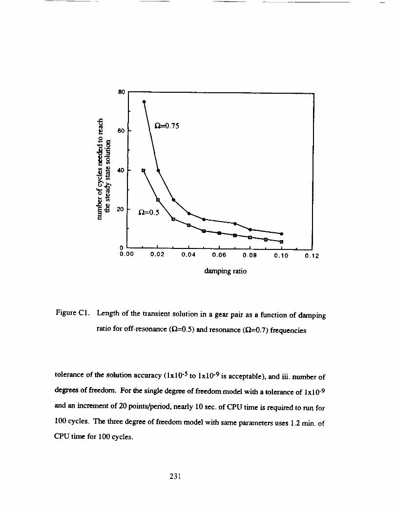
80
60
,o
20
0 I I I I I I I I m I •
0.00 0.02 0.04 0.06 0.08 0.10 0.12
damping ratio
Figure C 1. Length of the transient solution in a gear pair as a function of damping
ratio for off-resonance (D,---0.5) and resonance (_=0.7) frequencies
tolerance of the solution accuracy (lxl0 -5 to lxl0 -9 is acceptable), and iii. number of
degrees of freedom. For the single degree of freedom model with a tolerance of lxl0 -9
and an increment of 20 points/period, nearly 10 sec. of CPU time is required to run for
100 cycles. The three degree of freedom model with same parameters uses 1.2 rain. of
CPU time for 100 cycles.
231

APPENDIX D
COMPARISON OF PREDICTIONS WITH NASA MEASUREMENTS
In this section, a comparison of the FEM predictions of the NASA Gear Noise
Test Rig shown in Figure D1 with the measurements of NASA is given. System
parameters and the predicted natural modes of the system have already been given in
Tables 1.1 and 1.2, respectively. The static transmission error and mesh stiffness
variation predictions are also shown in Figure 4.8. Here, the comparison of the
predicted frequency response spectrum with measurements of NASA is limited to
torsional (angular acceleration) vibrations since the set-up was not equipped for
transverse vibration measurements. Only a qualitative agreement is observed between
the predictions and measurements as shown in Figure D2 due to the uncertainties
associated with the sensitivities of instruments and due to the errors involved in
measurement such as resonance and calibration problems of angular transducers.
coupling
/ N_ t°rquemeter l
motorshaft
F pinion !
-Jgear
gear box
Figure D1. NASA Gear Noise Test Rig.
232

(a)
f
0! • i
2_ 4_ 6_
0 2000 4000 6000
frequency (Hz)
Figure D2. Angular acceleration spectrum of the NASA Gear Noise Test Rig at pinion
location; a) measurements b) FEM predictions.
233

APPENDIX D
COMPARISON OF PREDICTIONS WITH NASA MEASUREMENTS
In this section, a comparison of the FEM predictions of the NASA Gear Noise
Test Rig shown in Figure D1 with the measurements by NASA is given. System
parameters and the predicted natureal modes of the system have already been given
in Tables 1.1 and 1.2, respectively. The static transmission error and mesh stiffness
variation predictions are also shown in Figure 4.8. Here, the comparison of the predicted
frequency response spectrum with measurements by NASA is limited to torsional
(angular acceleration) vibrations. Only a qualitative agreement is observed between
the predictions and measurements as shown in Figure D2. Quantitative discrepancies
are attributed to the resonance problems experienced with the angular transducers.
coupling
/ N'_ t°rquemeter
shaft ]
pinion
m
L gear
gear box
,_-.-bearing
load
Figure D1. NASA Gear Noise Test Rig.
234


Report Documentation PageNal_onal Aeronautics andS_ace Adm_nlsltatlon
1. Report No. NASA CR-4338 2 Government Accession No. 3, Recipient's Catalog No.
AVSCOM TR-90-C-020
4. Title and Subtitle
Non-Linear Dynamic Analysis of Geared Systems
7. Author(s)
Rajendra Singh, Donald R. Houser, and Ahmet Kahraman
9. Performing Organization Name and Address
Ohio State University
Department of Mechanical Engineering
Columbus, Ohio 43210
12. Sponsoring Agency Name and Address
Propulsion Directorate
U.S. Army Aviation Systems Command
Cleveland, Ohio 44135-3191
and
NASA Lewis Research Center
Cleveland, Ohio 44135-3191
5, Report Date
November 1990
6. Performing Organization Code
8. Performing Organization Report No.
None (E-5718)
10. Work Unit No.
505-63-51
11, Contract or Grant No.
NAG3-773
13. Type o1 Report and Period Covered
Contractor Report
Final
14. Sponsoring Agency Code
15. Supplementary Notes
Project Manager, James J. Zakrajsek, Propulsion Systems Division, NASA Lewis Research Center. This report is
based on a portion of the Ph.D. thesis of Ahmet Kahraman.
16. Abstract
Under the driving conditions, a typical gored system may be subjected to large dynamic loads. Also, the vibration level of the geared system
is direcdy related to the noise radiated from the gear box. Accordingly, a good understanding of the steady state dynanuc behavior of the system
is required in order to design reliable and quiet transmissions. It is the main focus of this study with the scope limited to a system containing
a spur gear pair with backlash and periodically time-varying mesh stiffness,and rolling element bearings with clearance type non-linearities.
The internal static transmission error excitation at the gear mesh, which is of importance from high frequency noise and vibration control
view point, is considered in the formulation in sinusoidal or periodic form. A dynamic finite element model of the linear time-invanant (LTI)
system is developed. Effects of several system parameters, such as torsional and transverse flexibilities of the shafts and prime mover/load
inertias, on free and forced vibration characteristics are investigated. Several reduced order LT1 models are developed and validated by
comparing their eigen solutions with the finite element model results. Using the reduced order formulations, a three-degree of freedom
dynamic model is developed which includes non-lineantics associated with radial clearances in the radial rolling element bearings, backlash
between a spur gear pair and periodically varying gear meshing stiffness. As a limiting case, a single degree of freedom model of the spur
gear pair with backlash is consider_l and mathematical conditions for tooth separation and back collision are defined. Both digital simulation
technique and analytical methods such as method of harmonic balance and the method of multiple scales have been used to develop the steady
state frequency response characteristics for various non-linear and/or time-varying cases. Difficulties associated with the determination of the
multiple solutions at a given frequency in the digital simulation tcchniqne have been resolved. The proposed formulation has been validated by
comparing the predictions with the results of two benchmark experiments reported in the literature. Several key system parameters such as
mean load and damping ratio are identified and their effects on the non-linear frequency response are evaluated quantitatively. Other funda-
mental issues such as the dynamic coupling between non-linear modes, dynamic interactions between component non-linear]ties and time-
varying mesh stiffness, and the existence of subharmonic and chaotic solutions including routes to chaos have also been examined in depth.
t7, Key Words (Suggested by Author(s))
Bearings
Gears
Vibrations
Machine design18, Distribution Statement
Unclassified - Unlimited
Subject Category 37
lg. Security Classif. (of this report)Unclassified } 2o, Security Classif. (of this page)Unclassified 1 21" N°" °f pages248
NASAFORM 1112(5OCT88 *For sale by the National Technical Information Service, Springfield, Virginia 22161
22. Price*
All
NASA-Langley, 1990


J_ .........
. • :_Z_!!_ _
_Z_ _
r
.... Z,, .........

_:_ =._, _iii__- .......___-_
Fostage ae Fees PaidNational Aeronautics andSpace AdministrationNASA-451
Official BusinessPenalty for Private Use 1300
Recommended


![MARINE DIESEL ENGINES Yanmar Saildrive SD20 Yanmar ...€¦ · Yanmar Saildrive Type SD25 Reduction gear system Constant mesh gear with dog clutch Reduction ratio [fwd/asn] 2.64/2.64](https://img.dokumen.tips/doc/110x75/6079f2b58c534c4ae36adf4c/marine-diesel-engines-yanmar-saildrive-sd20-yanmar-yanmar-saildrive-type-sd25.jpg)