
Quantification of the Immobilized Fraction
in Polymer Inorganic Nanocomposites
Dissertation
zur
Erlangung des akademischen Grades
doctor rerum naturalium (Dr. rer. nat.)
der Mathematisch-Naturwissenschaftlichen Fakultät
der Universität Rostock
vorgelegt von
Albert Sargsyan, geboren am 24. Juni 1980 in Jerewan,
Armenien
Rostock, 28 März 2007

Gutachter:
PD Dr. rer. nat. habil. Doris Pospiech, Leibniz-Institut für Polymerforschung Dresden Prof. Dr. Anahit Tonoyan, State Engineering University of Armenia Prof. Dr. Christoph Schick, Universität Rostock
Tag der Verteidigung:
11. Mai 2007

CONTENT
1. Introduction.................................................................................................. 5
2. Literature review .......................................................................................... 9
2.1. Polymer nanocomposites...................................................................... 9
2.1.1. Nanoparticles.................................................................................. 9
2.1.2. Preparation methods of polymer nanocomposites........................ 12
2.1.3. Morphology................................................................................... 17
2.1.4. Interfacial interactions................................................................... 19
2.1.5. Calorimetry ................................................................................... 23
2.2. Semicrystalline polymers .................................................................... 26
2.2.1. RAF in semicrystalline polymers................................................... 26
2.2.2. Vitrification of RAF........................................................................ 30
2.2.3. Devitrification of RAF.................................................................... 32
2.3. Heat capacity determination................................................................ 39
2.3.1. Linear scanning ............................................................................ 41
2.3.2. StepScan DSC ............................................................................. 44
3. Experimental.............................................................................................. 49
3.1. Materials ............................................................................................. 49
3.2. Preparation methods........................................................................... 53
3.2.1. Solution method............................................................................ 53
3.2.2. Shear mixing................................................................................. 54
3.2.3. Classical emulsion polymerization................................................ 54
3.2.4. Microemulsion polymerization ...................................................... 55
3.3. Characterization.................................................................................. 55
3.3.1. Gel permeation chromatography .................................................. 55
3.3.2. Electron Microscopy ..................................................................... 58

4
3.3.3. Small angle X-ray scattering..........................................................60
3.3.4. Thermogravimetry .........................................................................62
3.4. RAF determination ...............................................................................65
3.5. Annealing experiments.........................................................................66
4. Results........................................................................................................71
4.1. DSC measurements.............................................................................71
4.2. Specific heat capacity correction..........................................................75
4.3. RAF determination ...............................................................................84
4.4. Annealing experiments.........................................................................88
4.5. Devitrification of RAF at high temperature ...........................................94
4.5.1. StepScan DSC ..............................................................................94
4.5.2. High rate DSC ...............................................................................95
4.6. Plasticization experiments....................................................................95
5. Discussion ..................................................................................................99
6. Summary ..................................................................................................105
7. References ...............................................................................................107
Appendix........................................................................................................ A1
A1. Specific heat capacity data corrected .................................................. A1
A2. The calorimetric data from annealing experiments .............................. A3
A3. RAF layer thickness estimation ........................................................... A5

1. INTRODUCTION
Polymer nanocomposites have attracted a great deal of attention in
recent years due to their exceptional properties. Searching in SCOPUS™ [1]
for “polym* nanocompos* OR polymer inorganic hybrid” yields more than
8,000 hits from journals and more than 35,000 patents [2-17] and references
therein to name a few. Layered silicates [3], ceramic nanoparticles such as
silica and titania [18], carbon [19-21] and others are used as nanofillers.
Compared to conventional micro and macro composites the enormous surface
to volume ratio of the nanoparticles is the most important factor. The improved
properties of nanocomposites are related to the modification of the structure
and dynamics of the polymer at and near the particle surface. Because of the
large surface area this fraction of the polymer contributes significantly to the
properties of the whole nanocomposite, even at low filler content. In this
respect polymer nanocomposites are somehow similar to semicrystalline
polymers where the crystals can be considered as nanofillers too.
The glass transition, calorimetrically measured as well as the dynamic
glass transition studied by different probes (α-relaxation in amorphous
polymers), is often used to detect changes in molecular dynamics in polymers.
However, experimental results on polymer dynamics and the glass transition
in polymer nanocomposites are not conclusive concerning the mechanism and
the details of the modification near the particle surface. The glass transition
temperature of the nanocomposite was found to increase [22-28], to decrease
[27, 29-31], not to be influenced at all [22, 25, 27, 29, 32, 33] or the glass
transition disappeared totally [27, 34-36]. However, there are many
experimental results suggesting that the restriction of chain mobility caused by
the nanoparticles does not extend throughout the material but affects only the
chains within a few nanometers of the filler surface. The existence of such an
interfacial layer was shown for several filler polymer combinations by different
techniques [29, 32, 37-43]. In some cases the interfacial layer was identified
as totally immobilized [32, 35, 38] while in others a second glass transition [44,
45] was observed at higher temperature or at least a shoulder at the high
temperature flank of the relaxation peak [46]. The second peak observed in

6 Chapter 1
the mechanical tanδ curves by Eisenberg et al. [44, 45] was alternatively, as
an example to highlight the problem, interpreted as an indication for the
formation of a macroscopic gel in the studied nanocomposites [47] and not as
the glass transition of the interfacial layer as discussed in [44, 45]. Obviously a
peak in dynamic loss curves does not necessarily identify a glass transition.
Additional criteria must be fulfilled. A straight forward proof of a glass
transition is the observation of the typical step in heat capacity. This step like
change in heat capacity does not occur for local or normal mode relaxation
processes because of the missing contribution from entropy fluctuation [48-
50]. How important the length scale probed by the dynamic experiment for the
identification of a RAF is was demonstrated for semicrystalline poly(ethylene
terephthalate) (PET) [51, 52]. For the dynamic glass transition from dielectric,
dynamic mechanical and temperature modulated DSC an immobilized fraction
(rigid amorphous fraction (RAF)) was detected. In contrary, data from the
more local secondary ß-relaxation process were well described by a two
phase model not requiring the introduction of a RAF.
Even calorimetry, mainly Differential Scanning Calorimetry (DSC), is
routinely used to characterize nanocomposites often the glass transition
temperature was reported only. In a few other studies the shape of the glass
transition interval was investigated too [27, 32, 46, 53] or heat capacity was
measured quantitatively [42]. V.P. Privalko recognized very early the
importance of absolute heat capacity measurements for the thermodynamic
characterization of nanocomposites [25, 36]. Following these ideas heat
capacity measurements for poly(methyl methacrylate) (PMMA),
poly(butyl methacrylate) (PBMA) and polystyrene (PS) silicon oxide
nanocomposites of different morphology were performed. To identify an
immobilized interfacial fraction of the polymer we apply a formalism well
established for the determination of a rigid amorphous fraction (RAF) in
semicrystalline polymers as described by Wunderlich et al. [54, 55], was
applied.
For semicrystalline polymers there is an ongoing debate at what
temperature the immobilized fraction (RAF) devitrifies (relaxes), see e.g. [56-
58]. The question if the polymer crystals are melting first and simultaneously

Introduction 7
the RAF devitrifies or the RAF devitrifies first and later on the crystals melt can
not be answered easily on the example of semicrystalline polymers. This is
because the crystals, which are the reason for the immobilization of the
polymer, often disappear (melt) in the same temperature range as the RAF.
For polymer nanocomposites the situation is simpler. Silica nanoparticles do
not melt or undergo other phase transitions altering the polymer-nanoparticle
interaction in the temperature range where the polymer is thermally stable
(does not degrade). Therefore polymer silica nanocomposites are well suited
for a detailed study of the glass transition of an immobilized layer at the
interface between the polymer and the nanoparticle. Several authors claim to
observe such a second glass transition, see e.g. [44-46]. In all these cases the
second glass transition is detected as a separate peak or a shoulder of the α-
relaxation peak from dynamic measurements. But to the best of my
knowledge there is no evidence for a second glass transition in polymer
nanocomposites from calorimetric studies so far. It was therefore of interest to
obtain polymer nanocomposites with a significant amount of the immobilized
fraction and to measure heat capacity in order to detect a possible second
glass transition as an increase of heat capacity towards liquid heat capacity at
temperatures above the glass transition of the mobile polymer.

8 Chapter 1

2. LITERATURE REVIEW
2.1. Polymer nanocomposites
Filling polymers with inorganic particles is used to improve the stiffness
of the materials, to reinforce thermal and mechanical properties as well as the
chemical stability, to enhance the resistance to fire, decrease the gas
permeability etc. Due to the large surface area of the nanosized particles, its
dispersion in the polymers provides new properties or significantly improves
them in comparison to those of the pure polymer. The inorganic nanoparticles
uniform distribution in the polymer matrix generates a new class of materials
called polymer nanocomposites. The term hybrid composite or material is
commonly used as a synonym of organic inorganic nanocomposite. The
preparation of such materials dates back to 1990s when the first clay polymer
nanocomposite synthesis has been reported [59]. Kojima et al. found that
montmorillonite cation exchanged for 12-aminolauric acid was swollen by
epsilon-caprolactam to form a new intercalated compound. Caprolactam was
polymerized in the interlayer of montmorillonite, yielding a nylon 6-clay hybrid
(NCH). NCH is a nanocomposite of Nylon 6 and uniformly dispersed silicate
monolayers of montmorillonite. There are also many other nanoparticles used
to produce polymer nanocomposites depending on the properties which
should be improved [60-64]. Firstly the composites with layered silicates
(clays) are discussed, see [65] for a recent review.
2.1.1. Nanoparticles
The commonly used clays for formation of nanocomposites consist of
nanoplates of silicates. The thickness of the layers is usually in a range of
several nanometers and the length can be up to 1 μm or even more.
Formation of polymer-clay nanocomposites depends on the type of dispersion
of the silicate layers within the polymer matrix. There are three particular
cases of clay distribution: agglomerated stacks of the layers within the
polymer matrix, intercalated and exfoliated structures. Intercalated
nanocomposites are formed when the polymer chains penetrate between clay
plates or are polymerized there. However the lamellar structures of the clay

10 Chapter 2
still remain unbroken. When the plates are completely separated and have
random orientation in the polymer matrix, exfoliated nanocomposites are
obtained. The exfoliated structure is of particular interest because it increases
the polymer-clay interactions. The specific surface area of exfoliated clays is
usually of about 700 m2/g compared to 2 m2/g for the not exfoliated structure
[66]. Fig. (2.1) illustrates schematically the situation for these cases of polymer
clay nanocomposites: agglomerated, intercalated, partly intercalated and
exfoliated, and fully exfoliated. The agglomerated system is just a stack of the
silicate layers without polymer in between the layers. Fig. (2.1b) corresponds
to the polymer intercalated into the interlayer space situation.
(a) (b)
(c) (d)
Figure 2.1. The schematic of (a) – agglomerated, (b) – intercalated, (c) –
partly intercalated and exfoliated and (d) – exfoliated polymer
clay nanocomposites. The heavy straight lines are silicate layers,
the random thin lines are the polymer chains [65].
The fully exfoliated clay nanocomposite is shown in Fig. (2.1d) when all
clay layers are deagglomerated and dispersed independently on each other in

Literature review 11
the polymer matrix. The situation when both cases are present is illustrated in
Fig. (2.1c) which is also called intercalated-flocculated.
Clay based nanocomposites are currently synthesized and studied
most frequently. But nanoparticles of different shapes than layered silicates
are used to produce polymer nanocomposites as well. Nanoparticles of
spherical shape have attracted a great attention nowadays due to
enhancement of polymer properties. How complex the situation is can be
explained on the example of barrier properties. For layered silicate
nanocomposites barrier properties are normally improved. But in special
cases the addition of 10–30 wt% of nanosized fumed spherical silica to a
number of high-permeability polymers increases small penetrants permeation
by up to an order of magnitude [65, 67-71]. Normally, the addition of low-
permeability fillers (such as silica) reduces penetrant diffusion simply by
volume fraction effects. It is believed that the anomalous behavior observed
for nanosized particles is associated with the greater specific interfacial area
for the same level of loading compared to conventional (i.e., micron-sized or
larger) filler particles.
Another example is the production of composite biomaterials such as
bioresorbable polymers filled with spherical calcium phosphate nanoparticles
[72-78]. Calcium phosphate nanospheres mixed with poly(d,l-lactide-
coglycolide) intensifies the activity of alkaline phosphatase, which is important
for the differentiation of osteoblasts that dictate the regeneration process
within the organism. The most used calcium phosphate in implant materials is
hydroxyapatite, Ca10(PO4)6(OH)2, since it is the most similar material to the
mineral component of bones. Here nanocomposites with biocompatible
polymers are of special interest. These nanocomposites exhibit good
properties of biomaterials, such as biocompatibility, bioactivity,
osteoconductivity, direct bonding to bone, etc. [79, 80].
Nanotubes of different elements, its oxides etc. are widely used to
enhance the properties of polymers too. A nanotube is a nanometer scale
wire-like structure that is most often composed of carbon. A single walled
carbon nanotube is a one-atom thick sheet of graphite rolled up into a
seamless cylinder with diameter of the order of a nanometer. This results in an

12 Chapter 2
essentially one-dimensional nanostructure where the length-to-diameter ratio
exceeds 10 000. Such cylindrical carbon molecules have novel properties that
make them potentially useful in a wide variety of applications in
nanotechnology, electronics, optics and other fields of materials science. They
exhibit extraordinary strength and unique electrical properties, and are
efficient conductors of heat. Inorganic nanotubes have also been synthesized.
Inorganic nanotube is a cylindrical molecule often composed of metal oxides,
and morphologically similar to the carbon nanotube. They are observed to be
contained naturally in some mineral deposits too [21, 81-83]. In recent years,
nanotubes have been synthesised of many inorganic materials, such as
vanadium oxide and manganese oxide, and are being used for such
applications as redox catalysts and cathode materials for batteries. Inorganic
nanotubes are heavier than carbon nanotubes and not as strong under tensile
stress, but they are particularly strong under compression, leading to potential
applications in impact resistant applications such as bullet proof vests. The
name “nanotube” is derived from their size, since the diameter of a nanotube
differs from its length by six orders of magnitude. There are two main types of
nanotubes: single-walled nanotubes (SWNTs) and multi-walled nanotubes
(MWNTs). The specific surface area of the nanotubes and other particles of
nanosize is in the range of several hundreds m2/g similar to that of clays.
Due to the large surface area the nanoparticles tend to form
agglomerates of much larger size which suppresses its ability to enhance the
properties of the polymers while producing the composites. Therefore one of
the most important prerequisites of fabricating the polymer nanocomposites is
the deagglomeration of the nanoparticles. And the deagglomeration becomes
more difficult with increasing specific surface area. This is the main
disadvantage of using nanotubes to obtain composite materials because of its
larger surface area in comparison to nanosized clays and spheres.
2.1.2. Preparation methods of polymer nanocomposites
Several possibilities of deagglomeration are known which differ from
one preparation method to another. The preparation methods could be divided
into three widely used groups: (i) dispersion of nanoparticles into the polymer

Literature review 13
matrix, (ii) synthesis of the polymer in presence of nanofiller and (iii) the
synthesis of nanoparticles in presence of polymer.
To the first group belongs, for instance, the melt blending (or melt
compounding) of the polymer nanocomposites. It is processed typically in one
or two screw extruders at temperatures of the liquid state of polymer [23, 84-
87]. By control of mixing conditions the uniform distribution of the
nanoparticles in the polymer matrix can be achieved. The high shear forces
generated between extruder walls and screws make it sometimes possible to
obtain almost or full deagglomeration of the nanofiller added to the polymer.
This method is of technical importance because of the relatively simple
upgrade from laboratory to industrial scales. The disadvantage is that a
number of polymer chains may degrade due to the generated shear force or
high temperature. Control of molecular weight is therefore required. The
method is not technically available in our laboratory but the polymer
nanocomposites prepared by melt blending have been kindly provided by
colleagues at the Department of Polymer Structures, Leibniz Institute of
Polymer Research, Dresden.
Another way of producing polymer nanocomposites is the solution
preparation method (solution mixing) [88-91]. If the polymer can be solved and
the nanoparticles dispersed in a solvent, mixing brings reasonably good level
of dispersion of the nanoparticles in the polymer. In some cases even the
agglomeration tendency of the nanoparticles can be overcome. It is applicable
to polymers that can be dissolved or swelled by the solvent [92, 93]. The
deagglomeration of the nanoparticles may be reached by the mixing regimes
(intense stirring) as well as sonification of the solution.
Ultrasound is often used for the synthesis due to its influence on the
reaction [94-99]. The chemical effects of ultrasound derive primarily from
acoustic cavitation [100]. Bubble collapse in liquids results in an enormous
concentration of energy from the conversion of the kinetic energy of the liquid
motion into heating of the contents of the bubble. The high local temperatures
and pressures, combined with extraordinarily rapid cooling, provide a unique
means for dispersing nanoparticles or driving chemical reactions under
extreme conditions. A diverse set of applications of ultrasound to enhance

14 Chapter 2
chemical reactivity has been explored with important uses in synthetic
materials chemistry. For example, the sonochemical decomposition of volatile
organometallic precursors in low-volatility solvents produces nanostructured
materials in various forms with high catalytic activities. Nanostructured metals,
alloys, oxides, carbides and sulfides, nanometer colloids, and nanostructured
supported catalysts can all be prepared by this general route. But the main
advantage of this method in the context of the present work is the huge kinetic
energy which eventually is transferred to the nanoparticles resulting in
deagglomeration. Therefore the sonification is used to obtain polymer
nanocomposites during this work.
To the second group of preparation methods belong chemical
processes, in which polymerization is performed directly in the presence of the
inorganic particles. Examples of emulsion [35, 99, 101], miniemulsion [98,
102, 103], microemulsion [104, 105], suspension or dispersion [24, 106, 107]
polymerization, as well as differently performed free radical polymerization
[30, 108, 109] and ionic polymerization [110] etc. can be found in the literature
but emulsion polymerization is by far the technique most frequently used.
Heterogeneous polymerization, especially emulsion polymerization,
provides an effective way of synthesizing nanocomposites with various
architectures and forms [111]. Seeded (in the presence of nanoparticles)
emulsion polymerization technology is commonly used in the production of
nanocomposite emulsions. The seeded emulsion polymerization occurs
beforehand in the presence of water, emulsifier (surfactant), water soluble
initiator and a small amount of monomer, in which the emulsion has a large
number of particles with very small size. Then the polymerization reaction
continues in emulsion with the presence of the seeds (nanoparticles). This
method can control the reaction rate, particle size and morphology effectively
[112]. A number of papers deal with the encapsulation of sol–gel type metal
oxide particles (SiO2, TiO2) and other inorganic pigments [113] to give
organic–inorganic hybrid dispersions, where the polymer shell is built in situ by
means of conventional emulsion [35, 114], miniemulsion [115, 116] and
related dispersed-phase (Huang and Brittain 2001; Hwu, Ko et al. 2004)
polymerization processes. When the hydrophobic coat layer is simply
Literature review 15
adsorbed on the hydrophilic inorganic particle surface the poor chemical
interaction between the three phases (inorganic particle–hydrophobic
surfactant–organic polymer) can result in dewetting of the cover-forming
organic polymer. While the encapsulant in these organic–inorganic hybrids is
an organic polymer, the core inorganic particle usually presents a more
hydrophilic surface. Therefore, either the adsorption of the polymerization
initiator onto the particle surface through electrostatic interaction [117] or
special polymerization techniques are generally required when polymerization
onto an unmodified (i.e. not by surface-graft reaction hydrophobically
modified) inorganic particle is carried out by conventional emulsion process to
decrease the tendency to agglomerate.
Another way to keep the emulsion stable without using hydrophobic
modification or emulsifier is non-surfactant emulsion polymerization under
sonification. The idea is that the emulsion is formed by applying the
sonification and kept stable until the polymerization finished. Sonification of
the reaction media gives also the other advantage: inorganic nanoparticles are
kept deagglomerated up to the encapsulation by the polymer.
Frontal polymerization in the presence of nanofillers also belongs to the
second group of the preparation methods [118-120]. Frontal polymerization is
a process in which the polymerization propagates through the reaction vessel.
This approach allows producing the polymer nanocomposites by the
deagglomeration of the nanoparticles by an emulsifier in the reaction media
and then followed by radical polymerization in frontal regime. Frontal
polymerization is carried out usually in tubular reactors. Thermal frontal
polymerization begins when a heat source contacts a side of the tube and the
heat released by the exothermal polymerization initiates continuously next
portions of tube-like reaction media. This method allows the synthesis of
polymer nanocomposite materials which may have varying properties on the
product length scale of product.
The synthesis of nanoparticles in presence of monomers, oligomers or
polymers can be performed by different techniques. For instance, inorganic
(CdS, Ag)-polyacrylamide (PAM) nanocomposites can be prepared
successfully using a convenient ultraviolet irradiation technique; the initiation

16 Chapter 2
of reaction and polymerization are carried out by means of ultraviolet
irradiation [121]. It was found that the inorganic nanoparticles could be well
homogeneously dispersed in the polymer matrix because polymerization of
organic monomer and formation of inorganic nanoparticles were
simultaneous. It is very interesting that the presence of inorganic ions may be
favorable for the polymerization of the organic monomer. At the same time the
organic polymer matrices can efficiently prevent the produced inorganic
nanoparticles from agglomeration. The polymer nanocomposites can be
prepared also by synthesis of the nanoparticles in the polymer matrix [122-
124]. For instance, well-dispersed titanium dioxide (TiO2) nanoparticles were
synthesized utilizing a block copolymer as a template [125]. The nanoparticles
were confined within microphase separated domains of sulfonated styrene-b-
(ethylene-ran-butylene)-b-styrene (S-SEBS) block copolymers. Another
possibility is described in [126]. The formation of nanosized lanthanum
hydroxide particles in aqueous medium was carried out in the presence of
double-hydrophilic block copolymers. These copolymers contain a polyacrylic
acid block as an ionizable block, and a polyacrylamide (PAM) or a
polyhydroxyethylacrylate (PHEA) block as a neutral block. The nanoparticles
were synthesized by a two-step procedure. Firstly, the complexation of
lanthanum ions in water by the polyacrylate blocks induced the formation of
star-shaped micelles stabilized by the PAM or PHEA blocks. Secondly, the
inorganic polycondensation of lanthanum ions led to the formation of organic-
inorganic nanohybrids. Also here the organic polymer matrices efficiently
prevent the formed inorganic nanoparticles from agglomeration.
Consequently the polymer nanocomposites can be obtained by various
preparation methods. The properties of the composites depend on different
factors, such as nanoparticle size, the polymer type and most important on the
interaction between the polymer and the nanoparticles. One of the important
factors influencing on the composite properties is the degree of agglomeration
of nanoparticles in the polymer matrix. Therefore characterization of the
morphology of the nanocomposites obtained is an important task. Morphology
of the nanocomposites could be investigated by X-ray scattering or electron
microscopy and many other techniques.

Literature review 17
2.1.3. Morphology
Generally, the structure of polymer clay nanocomposites has typically
been studied using wide angle X-ray diffraction (WAXD) analysis and
transmission electron microscopic (TEM) observations. Due to its easiness
regarding sample preparation and availability WAXD is one of the commonly
used methods to probe nanocomposite structure [34, 127]. By monitoring the
position, shape, and intensity of the basal reflections from the distributed
silicate layers, the nanocomposite structure (intercalated or exfoliated) may be
identified. For example, in an exfoliated nanocomposite, the extensive layer
separation associated with the delamination of the original silicate layers in the
polymer matrix results eventually in the disappearance of any coherent X-ray
diffraction from the distributed silicate layers. On the other hand, for
intercalated nanocomposites, the finite layer expansion associated with the
polymer intercalation results in the appearance of new basal reflections
corresponding to the larger gallery height. Although WAXD offers a convenient
method to determine the interlayer spacing of the silicate layers in the original
layered silicates and in the intercalated nanocomposites (within 1–4 nm), little
can be said about the spatial distribution of the silicate layers or any structural
non-homogeneities in the nanocomposites.
Additionally, some layered silicates initially do not exhibit well-defined
basal reflections. Thus, peak broadening and intensity decrease are very
difficult to study systematically. Therefore, conclusions concerning the
mechanism of nanocomposites formation and their structure based solely on
WAXD patterns are only tentative. On the other hand, TEM allows a
qualitative understanding of the morphology, spatial distribution of the various
phases, and views of the defect structure through direct visualization.
Moreover TEM is used to characterize not only nanocomposites with layered
silicates but with the nanoparticles of any shape. However, special care must
be exercised to guarantee a representative cross-section of the sample and to
avoid artefacts. The WAXD patterns and corresponding TEM images of three
different types of nanocomposites are presented in Fig. (2.2). Both TEM and
WAXD are essential tools [128] for evaluating nanocomposite structure.
However, TEM is time-intensive, and only gives qualitative information on the

18 Chapter 2
sample as a whole, while low-angle peaks in WAXD allow quantification of
changes in layer spacing.
Figure 2.2. (left) WAXD patterns and (right) TEM images of three different
types of nanocomposites [65]
Typically, when layer spacing exceed 6–7 nm in intercalated
nanocomposites or when the layers become relatively disordered in exfoliated
nanocomposites, associated WAXD features weaken to the point of not being
useful. However, recent simultaneous small angle X-ray scattering (SAXS)
and WAXD studies yielded quantitative characterization of nanostructure and
crystallite structure in Nylon 6 based nanocomposites [129, 130].
As an example of electron microscopic characterization of
polymer/nanospheres composites TEM images of PMMA filled with silica are
represented in Fig. (2.3) [87]. Fig. (2.3a) shows the PMMA nanocomposites

Literature review 19
containing organically modified (PMMA grafted onto silica surface) while
Fig. (2.3b) non-modified silica nanoparticles dispersed in a PMMA matrix.
Figure 2.3. TEM images of PMMA/silica-gPMMA nanocomposites; (a) –
deagglomerated and uniformly dispersed, (b) – agglomerated
nanoparticles in polymer matrix (d(silica)=15-20 nm) [87]
It is seen that by grafting the PMMA onto silica surface one gets a
totally deagglomerated system while the unmodified nanoparticles appeared
to agglomerate into bigger particles.
The mentioned above reveals that there are several possibilities to
characterize the polymer nanocomposites morphology. Another important
parameter for polymer nanocomposites is the interfacial interaction between
the inorganic filler and the polymer. Different techniques are available for an
investigation of the properties of the polymer near the interface.
2.1.4. Interfacial interactions
The large specific surface area of the nanoparticles is important for
polymer properties in composites due to the interfacial interaction between
nanofiller and polymer matrix. Therefore it is of interest to investigate the
nature of such interactions. Several possibilities for the investigation of the
interface are known such as solid state nuclear-magnetic resonance (NMR)
[131-134], dynamic mechanical analysis (DMA) [37, 44, 133, 135-140],
nanoindentation [37, 141-143], infrared spectroscopy (IR) [35, 144], positron
annihilation spectroscopy [70, 145, 146], calorimetry (mainly differential
scanning calorimetry, DSC) [85, 87, 147, 148] and others.

20 Chapter 2
To investigate the interaction between nanofiller and polymer NMR
analysis is often used [131-133, 149-151]. In hybrid nylon 6/silica composites
nuclear relaxation measurements using low field NMR were applied [131]. The
NMR results showed that with up to 20% of silica there is compatibility due to
a weak intermolecular interaction. This may be concluded from the values of
spin-lattice relaxation time, which are in between the values of each initial
composite’s component. The data from NMR measurements also show that in
the Nylon 6/Si composites there is some interaction, as only two values of this
parameter were found for each Nylon 6/Si composition, and they were
different from pure nylon 6 and silica. The interphase behaviour of the cured
poly(amic acid) with polyhedral oligomeric silsesquioxane (POSS epoxide),
namely the octa(ethylcyclohexylepoxidedimethylsiloxy) silsesquioxane was
investigated by solid state NMR [133]. The results show that properties of the
interphase are varied systemically by adjusting the nanotether structure of the
epoxide molecules. Solid-state NMR data can be used also as a powerful tool
to characterize not only surfactant loading of the clays in polymer/layered
silicate composites but to obtain further insight into temperature-dependent
surfactant dynamics and structure of the surfactant layer too [132]. The NMR
measurements aimed at surfactant headgroups and tail ends supply
complementary information on the structure of that layer. It was found that two
microphases with different mobility and probably with different strength of the
attachment of surfactant headgroups to the silicate surface coexist over a
broad range of surfactant loadings and temperatures. By NMR analysis it was
possible to show that an excess of surfactant with respect to the cation
exchange capacity of the silicate causes plasticization of the surfactant layer
in pure organoclays and diminishes the tendency for intercalation.
Consequently NMR appears to be a very consistent tool to investigate the
interface interaction between polymer and nanofiller in composite materials.
But there is also a disadvantage of NMR use because this method
investigates mainly a behavior on a very local length scale and not necessarily
on the length scale representative for the glass transition.
Dynamic mechanical analysis is generally used to detect the property
enhancement of the polymer nanocomposites [139, 140] but also information

Literature review 21
about the influence of nanofillers on glass transition can be obtained.
Eisenberg et al. have investigated the interface for the different
polymer/inorganic filler nanocomposites using DMA [45]. The results showed
that interactions of polymer chains with silica nanoparticles restrict the mobility
of the chains at the interphase. Two peaks in the tanδ curves, one
corresponding to the common glass transition and a second peak at higher
temperature (Fig. 2.4a) were observed [45]. Fagiadakis et al. [46] found a
shoulder at the high temperature flank of the relaxation peak. Both findings
were interpreted as the glass transition of the immobilized polymer close to
the interphase.
(a) (b)
Figure 2.4. tan δ versus T - Tg curves for (a) - poly(styrene-co-4.5 mol %
sodium methacrylate) ionomer and the following polymers filled
with 10 wt% of 7 nm silica particles: PS, PMMA,
poly(4-vinylpyridine) and poly(vinylacetate) (the curves of the
filled polymers have been shifted for clarity by 0.2, 0.9, 1.4, and
1.9, respectively) [45] and (b) – styrene-4-vinylpyridine (S4VP)
copolymers of different vinylpyridine (VP) contents, but
containing 20 wt% silica [44].
The second peak observed in the mechanical tanδ curves by Eisenberg
et al. [44, 45] was alternatively, as an example to highlight the problem,

22 Chapter 2
interpreted as an indication for the formation of a macroscopic gel in the
studied nanocomposites [47] and not as the glass transition of the interfacial
layer as in [44, 45]. Obviously a peak in a dynamic loss curve does not
necessarily identify the occurrence of a glass transition, additional criteria
must be fulfilled. The first peak in Fig. (2.4) for all systems is assigned as a
conventional glass transition because it is present also in pure polymers. It is
important to mention that the second peak in the tan δ curve for PS/10 wt%
silica nanocomposites in Fig. (2.4a) does not appear for the similar system but
filled with 20 wt% filler (the curve which corresponds to 0 wt% VP in
Fig. (2.4b)). Anyway in Fig. (2.4b) the second peak in the dynamic loss curve
is present only for the S4VP copolymers. This means that this peak appears
most likely due to the interaction between nanoparticles and VP, but not PS.
However the second peak in Fig. (2.4a) cannot be explained by this
assumption because the polymer used for the PS/SiO2 nanocomposites
preparation was pure PS which seems to exhibit no interaction with silica
nanoparticles. Anyway, the situation here could be clarified having the results
of the measurement at the exactly same conditions for silica used. The silica
nanoparticles might have an organic cover on its surface which may exhibit
the peak in the tanδ curve. Consequently it is difficult to draw final conclusions
about the mobility of the interfacial polymer layer for the pure polystyrene
silica nanocomposites by DMA. This problem will be discussed in Chapter (4).
The study of organic phase mobility in organic-inorganic coatings by
DMA is reported in [139]. The analysis of the hybrids coated on a PET film
(coating thickness 10 μm and 40 μm) shows an additional up-shift of glass
transition temperature, more markedly in the case of the thinner hybrid
coating. This result is attributed to molecular interactions at the
substrate-coating interface that locally hinder molecular mobility. The
consequent increase of glass transition temperature is more evident when the
coating layer is thin.
The chain mobility in the polymer-clay nanocomposites is greatly
reduced as studied by dynamic mechanical analysis (DMA) and dielectric
analysis (DEA) in [140]. The modulus of the composite increases significantly.
The modulus enhancement strongly relates to the volume of the added clay as

Literature review 23
well as the volume of the constrained polymer. This modulus enhancement
follows a power law with the content of the clay in the composite. This
study [140] also indicates that the structure of clay nanocomposites with
strong interfacial interactions is analogous to that of semicrystalline polymers.
In the case of polymer-clay nanocomposites, the intercalated clay phase
serves as an unmeltable crystalline phase which results in improvement in
mechanical and thermal properties. The same consideration can be applied
for the other polymer/inorganic nanofiller systems.
The nanoindentation measurements could be revealed as an
appropriate technique to characterize hybrid organic–inorganic thin films [37,
142] which obviously exhibits very similar mechanical and thermal properties
to those of interfacial polymer layer in composite materials. The indentation
study shows that the extent of the hybrid interface could be adjusted by the
use of preformed silica nanoparticles. It was also shown that the mechanical
response was governed by the size of the hybrid interface since the
mechanical properties of materials based on sol–gel silica are more elevated
than those obtained from materials formed from silica nanoparticles which
exhibit a more defined interface. Therefore to allow the precise quantification
of the nanofiller surface area in polymer nanocomposites spherical silica
nanoparticles has been used for the present work.
2.1.5. Calorimetry
Privalko et al. have consistently investigated the interfacial organic
layer mobility for different hybrid materials using calorimetric methods [22, 25,
152-155]. The heat capacity of polyurethane filled with finely dispersed Aerosil
(specific surface area is 175 m2/g) was studied as a function of temperature in
[156]. The addition of filler was found to decrease the crystallinity of the filled
polyurethane and significantly reduce enthalpy of the polymer. This is
explained by the appearance of macromolecules with reduced mobility in the
amorphous zones at the polymer-particle interface. The calorimetric study of
oligo-ethylene glycol adipate (OEGA) filled with Aerosil and colloidal graphite
(calculated specific surface area is 0.67 m2/g) showed an interesting result
(Fig. (2.5)) [36]. In Fig. (2.5) the specific heat capacity as a function of
temperature for quenched samples of differently filled OEGA is presented.

24 Chapter 2
Figure 2.5. The heat capacity of quenched samples of filled OEGA. Filler
contents (wt %): 1 – 0, 2 (filled triangle) – 1, 3 – 50 graphite, 4 –
10 Aerosil [36].
It is seen that at 50 wt% graphite loading the glass transition of the
OEGA disappears. The same can be observed for Aerosil filled sample but
already at much lower filler content. The reason for that could be the
difference in specific surface area of the inorganic fillers. Consequently,
Fig. (2.5) [36] clearly demonstrates that the interfacial organic layer shows
much lower mobility in comparison to that of the pure (unfilled) substance,
which at relatively high filler concentrations can result in disappearance of the
step in heat capacity at glass transition.
Later authors confirmed [25] that the properties of filled polymer
systems are determined by the amount of the interfacial layer. The heat
capacity data from the calorimetric measurements indicated that an increase
in Aerosil content results in a more or less reduction of calorimetric relaxation
strength at the glass transition temperature. It has to be mentioned that in [25]
only the polymer was varied in polymer/filler hybrids to get comparable data
for each system. A calorimetric study of PMMA and PS filled with powdered
glass [22] confirmed the tendency of the mobility decrease of the interfacial
organic layer for these systems with increasing filler content. The glass
transition temperature was found to increase with increasing powder content.
It was also shown that the absolute values of the specific heat capacity of

Literature review 25
composites are smaller than those of unfilled polymers not only in solid but
also in liquid states. The difference in solid state is thought to disappear in a
high enough temperature range owing an intensification of the
macromolecular thermal vibrations but however it was not clearly
detected [22]. These works, for the first time, show the possibility to
investigate the interface in polymer nanocomposites calorimetrically.
Giannelis et al. have investigated polymer silicate composites by
different methods as well as DSC [34]. It was shown that on a local scale,
intercalated polymers exhibit relaxation for a wide range of temperatures, with
a significant suppression (or even absence) of cooperative dynamics typically
associated with the glass transition. The glass transition temperature of
polystyrene filled with organically modified silicate (C18FH) was reported also
to disappear. Namely, the absence of any thermal transition for the
intercalated polymer in the conventional glass transition temperature region
was observed similar to [36]. For the polyimides with silicate obtained by
sol-gel method no glass transition was detected in data from DSC
measurements at 50 wt% nanofiller loading [27]. One has to mention that the
absence of the step in glass transition temperature range was observed only
for the polymer with relatively low molecular weight (5000 g/mol) while for the
systems with higher molecular weight the calorimetric relaxation strength was
only lowered. Taking these results into consideration, the polymers to be
chosen for the investigation in this work were synthesized with a wide
molecular weight distribution. The low molecular weight fraction is expected to
interact with nanoparticles easier than that of high molecular weight.
On the contrary to the mentioned above, the glass transition was
reported also not to be influenced et al. [22, 25, 27, 29, 32], to be shifted to
higher [22-28] or lower [29, 30] temperatures as well.
The interfacial interaction can be varied by the preparation method of
the polymer nanocomposites, by change of nanoparticles type, dimensions,
surface modification and polymer type as reported in literature. Reviewing the
investigations of the interfacial layer in polymer nanocomposites one may
conclude that this is still an open question. However it is generally reported
that in polymer nanocomposites the polymer layer on the nanoparticle surface

26 Chapter 2
is thought to be immobilized, e.g. the chain mobility is reduced, in spite of rare
situations as in [31, 138, 149] for instance or in the others given in the
introduction. But to the best of my knowledge, there is no evidence of DSC
confirmation of the interfacial immobilization of the polymer by nanofiller where
the nanoparticles surface is not organically treated.
2.2. Semicrystalline polymers
A similar situation, a polymer interacting with rigid particles, is present
in semicrystalline polymers. Semicrystalline polymers consist of crystallites
(lamellae) and an amorphous fraction which thickness is in the range of
ca. 10 nm. The polymer nanocomposites are usually filled with particles of
similar size. Therefore the interface between amorphous and crystalline
fractions in the semicrystalline polymers can be treated in the same way as for
polymer nanocomposites if an immobilized layer exists.
The quantification of the immobilized amorphous polymer by the
crystals, i.e. a rigid amorphous fraction (RAF), was introduced for
semicrystalline polymers [51, 157, 158], see Wunderlich for a recent
review [55]. Similar procedure may be performed for the polymer
nanocomposites as well. Consequently the amount of immobilized layer may
be available from the calorimetric measurements as described in [157]. The
understanding of its formation and devitrification both in semicrystalline
polymers and polymer nanocomposites can help to obtain materials with
controlled properties.
2.2.1. RAF in semicrystalline polymers
Semicrystalline polymers have frequently a negative contribution to the
heat capacity between glass transition and melting, linked to the RAF [55].
Because of the need to accommodate flexible polymer molecules of typically
1–100 μm length into micro- and nanophases, there is usually a strong
coupling between crystal and amorphous phases due to the frequent crossing
of the interface by the long molecules. In all polymers, this strong coupling
between the phases results in a broadening of the glass transition to higher
temperature, as seen for instance for PET [159, 160]. In many polymers this
coupling causes a separate glass transition for the RAF, as summarized

Literature review 27
in [55]. An effect due to the RAF was first reported for several semicrystalline
polymers as a deficit in calorimetric relaxation strength (Δcp) at glass
transition [157, 161].
The heat capacity of the semicrystalline poly(oxymethylene)s between
the glass transition and the melting temperature, as shown in [157], indicated
much lower levels than expected from a two-phase crystallinity model as
shown in Fig. (2.6). The dashed line in Fig. (2.6) corresponds to liquid
poly(oxymethylene) heat capacity and the dotted line is a guess at the low
temperature continuation. The heavy line is the experimental data presented.
The dash-dotted lines correspond to the calculated data for the indicated
percentages of “rigid” phase.
Figure 2.6. Heat capacity of poly(oxymethylene) when fitted assuming 56%
crystallinity, 24% rigid amorphous, and 20% mobile amorphous
poly(oxymethylene). The dashed line correspond to liquid
poly(oxymethylene) heat capacity, the dotted line is a guess at
the low temperature continuation. The heavy line is the
experimental data. The dash-dotted lines represent calculated
data for the indicated percentages of “rigid” phase (crystalline
and rigid amorphous). Only the 80% curve fits the data [157]

28 Chapter 2
The authors showed that the straight lines of Fig. (2.6) are tangents to
the 100% crystalline samples [157]. A larger rigid fraction (0.8) than calculated
from crystallinity (0.56 for Fig. (2.6)) according to the two-phase model was
needed to match experimental data and calculation. The experimental data lie
significantly lower than the calculated data from the two-phase model. This
means that there is a part in rigid fraction which does not contribute to the step
in heat capacity at glass transition. And the same situation was found for the
other poly(oxymethylene)s investigated [157].
In addition, in [157] the data for chemically different samples felt on
slightly different curves. The only interpretation of those results could be that
the crystallinity model is not suitable for the description of heat capacities of
poly(oxymethylene) in this temperature range. To derive a possible structure
parameter for heat capacity the authors assumed that, based on the normal
beginning of the glass transition, a portion of the non-crystalline fraction is
gaining normal mobility at the glass transition. This part of the non-crystalline
fraction was called “mobile amorphous” and treated similar to the super cooled
liquid, with a heat capacity identical to the data extrapolated from the melt.
Figure 2.7. Subdivision of the heat capacity cp of semicrystalline
poly(oxymethylene) into “rigid amorphous” and “mobile
amorphous” at 265 K [157]
The remaining non-crystalline fraction of the sample, which was called
“rigid amorphous”, was assumed to depend on sample structure, and possibly
Literature review 29
also on crystallization condition, see Fig. (2.7). One has also to mention that
the curves calculated using the crystallinity from the heat of fusion as a
calculated parameter (0.56) are far out of any reasonable experimental
uncertainty. The negative and positive heat capacity deviations for 38
semicrystalline poly(oxymethylene)s and poly(oxyethylene)s in the
temperature range between glass and melting transition have been clearly
delineated in [157]. The negative deviation was linked to an added fraction of
RAF, while the positive deviation was assigned to processes such as defect
formation or beginning of melting, i. e. gaining of mobility and possibly
disordering. The RAF in poly(oxymethylene) was found to be constant up to
the melting region, in contrast to polypropylene, where it is decreasing with
increasing temperature [157].
The concept of a rigid amorphous fraction can also be applied for other
relaxation strength measurements than heat capacity. Mechanical [162, 163]
and dielectric spectroscopy result in nearly the same RAF as determined from
heat capacity increments [52, 164]. From the dielectric data not only the
relaxation strength at the dynamic glass transition but also the relaxation
strength for the secondary (more local) relaxations is available. Dobbertin et
al. [52] report about calorimetric and dielectric measurements on the same
semicrystalline PET samples. The question arises if the β-relaxation
(connected with local movements) is similarly influenced by the crystals than
the dynamic glass transition? Such local movements are not possible in the
crystalline part but could be expected to occur in the whole non-crystalline
part. Fig. (2.8) compares the normalized dielectric intensities for the α- and
β-relaxation and the α-relaxation strength from calorimetric measurements.
This confirms the introduction of RAF in semicrystalline polymers, i.e. that the
deviations from the two-phase model for the α-relaxation are present in the
dielectric data too. In [52] the authors found that the secondary β-relaxation
follows the two–phase model as shown in Fig. (2.8). This means that a local
movement is possible in the RAF but not a cooperative segmental motion
(α-relaxation, glass transition).

30 Chapter 2
Figure 2.8. Normalized intensity for α (ε, cp) and β (ε) for differently
crystallized PET samples [52]
Obviously the length scale probed by the different measurements is
different and yields different outcomes regarding the existence of a RAF. The
results of further investigations from the dielectric relaxation and calorimetry
allowed authors to conclude that both independent measurements yield a
correlation length of some nm for the undisturbed glass transition. This allows
concluding that the RAF layer thickness should be most likely in the same
range in the semicrystalline polymers and possibly also polymer
nanocomposites.
2.2.2. Vitrification of RAF
The mentioned above reveals that the RAF existence in semicrystalline
polymers is already confirmed by different methods. Of interest is the question
when the RAF is formed. Fig. (2.9) represents the results from
quasiisothermal crystallization measurements of two polymers [165]. As seen
in Fig. (2.9) the measured heat capacity becomes smaller than the baseline
heat capacity according the two-phase model (curve d), indicating the
occurrence of significant RAF during the crystallization process. On the other
hand, the expected heat capacity, taking into account the RAF obtained at the
glass transition (line e) is in perfect agreement with the measured value at the
end of isothermal crystallization. There is no difference in the amount of RAF
at crystallization and the glass transition temperature; also Tg is more than

Literature review 31
30 K below the crystallization temperature in the case of polycarbonate (PC).
Therefore, one can conclude that the total RAF of PC and
poly(3-hydroxybutyrate) PHB is vitrified (formed) during the isothermal
crystallization. No additional vitrification occurs on cooling from the
crystallization to the glass transition temperature.
(a) (b)
Figure 2.9. Time evolution of heat capacity during quasiisothermal
crystallization of (a) - PC at 456.8 K and (b) – of PHB at 296 K,
temperature amplitude 0.5 K and period 100 s, curve a. Curves b
and c correspond to solid and liquid heat capacities from the
ATHAS database [166], respectively. Curve d was estimated
from a two-phase model and curve e from a three-phase model.
The squares represent measurements at modulation periods
ranging (a) – 30 to 12 000 s and (b) – 240 to 1 200 s. Curve f
shows the exothermal effect in the total heat flow rate [165]
Cebe et al. have investigated the formation of the RAF for isotactic
polystyrene (iPS) [167]. The cold crystallization of iPS resulted in the
formation of an RAF, which increases with crystallization time and
temperature in a manner analogous to the development of the crystalline
fraction. Authors conclude that the RAF is formed at nearly the same time as
the crystalline phase and increases more rapidly after spherulite impingement.
Consequently the formation (vitrification) of RAF can be followed by
calorimetric methods. But there are cases when vitrification can not be
determined from heat capacity. For instance, the reversing melting occurring

32 Chapter 2
during the quasiisothermal crystallization of poly(ether ether ketone) (PEEK)
as discussed in [168].
Figure 2.10. Specific heat capacity of PEEK as a function of time from the
data shown in [168]. Curve a - cp value from the measured heat
flow rate, b - expected baseline heat capacity.
In Fig. (2.10) the measured complex heat capacity and expected
baseline heat capacity are shown. In case of PEEK complex heat capacity
increases during crystallization, while baseline heat capacity decreases. If one
wants to study crystallization by TMDSC measurement conditions must be
chosen to fulfill requirements of linearity and stationarity as discussed in [169,
170]. Changes in sample properties (e.g. degree of crystallinity) must be
negligible during one modulation period. But even if these conditions are
fulfilled melting and subsequent crystallization may occur during one period of
the temperature modulation and contribute to the measured heat capacity.
Finally, an excess heat capacity can be seen. Fig. (2.10) shows that the
measured heat capacity behaves different from the expected baseline heat
capacity with increasing crystallinity. The difference can be described as an
excess heat capacity which stays constant after the end of main
crystallization. It can be related to reversing melting during crystallization
[168].
2.2.3. Devitrification of RAF
In spite of the rare situations like described for PEEK the vitrification of
the RAF in semicrystalline polymers can be followed by isothermal

Literature review 33
crystallization. The question arises, at which temperature the RAF devitrifies.
Quantitative DSC and TMDSC are the key macroscopic techniques which
allow the characterization of the intermediate phase by evaluation of the glass
transition, the quantitative evaluation of the amount of a RAF, and the
differentiation of various types of RAF via its separate Tg below, at, or above
Tm [55]. Since the main temperature range for characterization lies between Tg
and Tm, a range where the increase in heat capacity due to conformational
motion can compensate the decrease due to the RAF, and where its increase
due to the RAF glass transition may be competing with the beginning of
melting and reorganization of crystals and of reversible melting. Therefore to
detect when the RAF devitrifies calorimetrically is a very difficult task. Special
techniques like quasiisothermal TMDSC and frequency- and amplitude-
dependent measurements need to be tried to avoid the problems mentioned.
The problem of reversible melting is introduced in more detail in [160].
Quasi-isothermal TMDSC in the melting range should, according to [160],
have no contribution from melting and/or crystallization to the reversing heat
capacity. Fig. (2.11) shows, however, that this is not the case. A reversing
contribution to the heat capacity is present and depends on the crystallization
conditions. Although the contribution is much less than that of the total heat of
fusion, the reversing contribution is not negligible. The only interpretation of
this observation is that the polymer molecules that contribute to the reversing
heat capacity are still attached to crystals that melt at a higher temperature
and can serve as molecular nuclei. After the heating cycle a number of melted
polymer molecules, which are still attached to higher melting crystals can
recrystallize during the cooling cycle with negligible supercooling. Overall, this
process yields a reversible, apparent heat capacity contribution similar to
[168].

34 Chapter 2
(a) (b)
Figure 2.11. Reversing heat capacity by quasi-isothermal TMDSC (a) - on
cooling from the melt (filled circles) and (b) - on heating from the
quenched, amorphous sample. The thin lines indicate the
ATHAS database data [166] for the amorphous and crystalline
PET; the broken lines indicate the computed heat capacity for
(a) - 49% and (b) – 40% crystalline PET. The open circles are
melt-crystallized PET on the quasi-isothermal upon step-heating
as reference [160]
The RAF is the part of the non-crystalline PET that does not participate
in the measured Δcp at the glass transition but, on the other hand, does also
not contribute to the heat of fusion [157]. The figure shows that the reversing
heat capacities reach the expected equilibrium heat capacity of the
semicrystalline PET derived from the ATHAS database [166] at about 430 to
450 K. Unfortunately, this temperature is sufficiently close to the beginning of
melting that the actual crossover temperature may be somewhat higher due to
some low temperature reversible melting. And such problems limit the
possibilities of the RAF devitrification detection.
Wunderlich et al. however discussed the RAF determination for the
special case where the limitations mentioned above do not appear as a
disturbing factor. For the understanding of the mechanism of formation and
devitrification of the RAF the quasi-isothermal TMDSC of poly(oxy-2,6-

Literature review 35
dimethyl-1,4-phenylene) (PPO) is described in [171]. In Fig. (2.12) the
measured, reversing heat capacity and the crystallinity of PPO are plotted
together.
Figure 2.12. Comparison of the measured heat capacity of semicrystalline
PPO with its change in crystallinity and RAF [171]
As the temperature increases the crystallinity and the RAF decrease,
but at different rates. melting is completed at about 510 K. Up to about 495 K
the crystallinity decreases very little, while the RAF loses almost 20% of its
value, which is in accordance with the assumption that the surrounding glass
must become mobile first, before melting can occur. Between 495 and 510 K
the decrease of both, the RAF and the crystallinity, is close to linear, with the
RAF losing three times as much solid fraction as the crystallinity. In this
temperature range the crystallinity is lost parallel to the loss of the RAF.
Cebe et al. offered a mechanism of RAF devitrification for iPS [172].
Taking into consideration the formation of RAF at crystallization
temperature (Tc), the authors pointed out that RAF is stable at temperatures
below Tc. [56]. Furthermore, heat capacity measurements above the melting
point suggest that only one phase exists at high temperature, i.e. 100% liquid
mobile amorphous fraction (MAF), i.e. not immobilized amorphous polymer.
Therefore, the RAF must be relaxed at some temperature between Tc and the
upper melting point. To provide further evidence for devitrification of RAF,
Fig. (2.13b) shows the temperature dependent heat capacity data in expanded
scaling, for Tc = 155 °C, and for predictions based on the three-phase model

36 Chapter 2
(dark solid curve). Also shown are the predictions based on a two-phase
model (light solid curve). In Fig. (2.13b) at temperatures below the annealing
peak, experimental heat capacity data matches the three-phase model
baseline. At temperature just above the annealing peak, the system
approaches to the two-phase model, in which only crystals and liquid (MAF)
exist. Thus, as temperature increases from below Ta to above Ta, the system
exhibits a transition from three-phase to two-phase. Such a transition turns the
RAF into an identical amount of MAF.
Figure 2.13. Standard DSC scan ((a) – wide scaling, (b) – expanded scaling)
showing specific heat capacity vs. temperature at heating rate of
10 K/min for iPS cold-crystallized at 155 °C for 12 h. The dashed
line is the heat capacity of 100% liquid, while the dotted line is
the heat capacity of 100% solid obtained from the ATHAS
database [166]. In part (a) the solid line and in part (b) the dark
solid line represents the baseline heat capacity based on the
three-phase model, while the light solid line indicates the
baseline heat capacity based on the two-phase model [56, 172,
173]
Using Fourier-Transformation-Infrared spectroscopy (FTIR), wide angle
X-ray scattering (WAXS), and standard DSC scanning, the crystalline fraction
appears to be unaffected by the transition of RAF into MAF, at least within the
error limits of the crystallinity measurement [172]. It is possible that a tiny
amount of crystals, within the error limits, melts at Ta. However, as the authors
demonstrated that it is not possible for the entire endotherm area at Ta to arise
from crystal melting. Therefore, the authors assign the annealing peak in
Fig. (2.13a) as the devitrification of the rigid amorphous fraction, which

Literature review 37
transforms RAF into equilibrium liquid without detectable melting of the
crystals. They assume that the relaxation of RAF occurs as a sigmoidal
change in the baseline heat capacity, accompanied by an excess enthalpy.
But the assumption of RAF devitrification by [172] was disproved later
by Minakov et al. using high-rate calorimetry [57].
Figure 2.14. Heat capacity of iPS sample crystallized at 140 °C for 12 h at
heating rate 10 K/min (dashed line) and 30,000 K/min (solid line)
[57]. Expected heat capacities [166] for the liquid, the crystalline
and the semicrystalline iPS according a two- and three-phase
model.
In order to check the hypothesis by Cebe et al. the authors compare in
Fig. (2.14) heat capacities at slow and fast heating, 10 K/min and
30 000 K/min, for the iPS sample crystallized at 140 °C. For both heating rates
above glass transition heat capacity follows the line expected from a three-
phase model taking into account crystalline, mobile amorphous and rigid
amorphous fractions, for details see e.g. [56, 165, 167]. For the low heating
rate after the first endothermic peak heat capacity coincides with that
expected according a two-phase model taking into account crystalline and
mobile amorphous fractions only as already shown by Cebe et al. [56]. If the
first endothermic peak is caused by an enthalpic relaxation of the RAF one
would expect to see a similar effect or at least some step in the heat capacity

38 Chapter 2
curve at temperatures around 160 °C for the fast heating too. But there is
nothing to see at fast heating. Heat capacity reaches the liquid line above the
single melting peak. This indicates that melting of crystals and relaxation of
the RAF occurs in the temperature range of the broad single melting peak,
most probably simultaneously. There is a solid fraction of about 0.55 as for the
slowly heated sample, which is indicated by the three-phase line in Fig. (2.11),
[57]. At fast heating one sees a significant shift of the glass transition to higher
temperatures. The Tg of the mobile amorphous fraction shifts from 100 °C at
10 K/min to about 115 °C at 30 000 K/min. Considering the same apparent
activation energy for the relaxation of the RAF, the beginning of the heat
capacity increase (peak or step) should be shifted to 160 °C. But on fast
heating nothing special happens around 160 °C. It is therefore unlikely that the
annealing peak is related to the nonreversing enthalpic relaxation of the RAF
only. As shown for PC and PHB [165] and for iPS [56] heat capacity changes
from the value expected from a three-phase model to that according a
two-phase model in the temperature range of the low temperature endotherm.
Combining these earlier observations with a continuous melting–
recrystallization–remelting model, which is supported by the results obtained
by Strobl et al. [174, 175] too and the fast heating experiments, one can
discuss the observations as follows. At low heating rates melting of the
crystals starts at the rising flank of the lowest temperature endotherm. Parallel
to crystal melting the RAF surrounding the just molten crystals relaxes. As
shown in [58, 176] the melt is than in a state (conformation) allowing very
rapid (within milliseconds) recrystallization. This recrystallization creates more
stable crystals but does not significantly change overall crystallinity. Assuming
a continuous melting–recrystallization–remelting the remaining amorphous
material in between the crystals may not be vitrified as in the case of slow
isothermal crystallization [56, 165]. If the amorphous material does not vitrify
heat capacity should be the same as expected from a two-phase model as
soon as the continuous melting–recrystallization–remelting starts and that
seems to be what is observed [57].
The mentioned above demonstrates that the question, at which
temperature the RAF devitrifies, is still under discussion. However Wunderlich

Literature review 39
et al. discussed the relaxation of RAF in semicrystalline polymer (PPO) using
TMDSC which is a special case when the difficulties like beginning of the
melting, reorganization or reversing melting do not arise. In this work I tried to
find a solution by means of a model system – polymer nanocomposites. It is
hoped that absence of any transition of inorganic fraction in the range from Tg
up to the degradation temperature of the truly amorphous polymer will help to
avoid the difficulties occurring for semicrystalline polymers. For that one has
first to obtain the polymer nanocomposites exhibiting a RAF. Next the RAF
should be quantified in the same way as for semicrystalline polymers from
heat capacity data as shown in [157]. Then the devitrification of the RAF could
be investigated by increasing mobility of the polymer chains of the RAF by
increasing temperature or adding some plasticizer. For the two later points
heat capacity must be determined with adequate precision
2.3. Heat capacity determination
Heat capacity of polymeric materials can be measured by calorimetry.
The applications and interest in calorimetry in material science have grown
enormously during the last half of the 20th century and the beginning of the
21st. Different calorimetric methods are utilized to get information about the
thermal properties of the materials, such as adiabatic [177], AC [178, 179],
DSC [180-182] and TMDSC [183-191]. But the DSC and TMDSC are used in
this work due to the simplicity of use and the uncertainty in measurement
results of ca. 2% or even better [192].
Two basic types of differential scanning calorimeters must be
distinguished:
• Heat flux DSC
• Power compensation DSC.
They differ in the design and measuring principle. Common to all DSCs is a
differential method of measurement which is defined as follows: A method of
measurement in which the measured quantity (measurand) is compared with
a quantity of the same kind, of known value only slightly different from the
value of the measurand, and in which the difference between the two values is
measured [193].

40 Chapter 2
The characteristic feature of all DSC measuring systems is the
twin-type design and the direct in-difference connection of the two measuring
systems which are of the same kind.
The heat flux DSC belongs to the class of heat-exchanging
calorimeters [181]. In heat flux DSCs a defined exchange of the heat to be
measured with the environment takes place via a well-defined heat conduction
path with given thermal resistance. The primary measurement signal is a
temperature difference; it determines the intensity of the exchange and the
resulting heat flow rate (Φ) is proportional to it. In commercial heat flux DSCs,
the heat exchange path is realized in different ways, but always with the
measuring system being sufficiently dominating compared to the heat transfer
inside the sample.
The power compensation DSC belongs to the class of
heat-compensating calorimeters [181]. The heat to be measured is (almost
totally) compensated with electric energy, by increasing or decreasing an
adjustable Joule’s heat.
Figure 2.15. Power compensation DSC (Perkin Elmer Instruments). Set-up of
the measuring system. Sample measuring system with sample
crucible, microfurnace and lid, reference sample system
(analogous to sample), 1 heating wire, 2 resistance
thermometer. Both measuring systems, separated from each
other, are positioned in a surrounding (block) at constant
temperature.
Sample ReferencePlatinum Alloy
PRT Sensor
PlatinumResistance Heater
Heat Sink
SampleSample ReferenceReferencePlatinum Alloy
PRT Sensor
PlatinumResistance Heater
Heat Sink
(1)
(2)

Literature review 41
Since the DSC used for this work is a power compensation DSC the
measuring system of it (Perkin Elmer DSC) is described in more details. The
measuring system (Fig. (2.15)) consists of two identical microfurnaces which
are mounted inside a thermostated aluminium block. The furnaces are made
of a platinum-iridium alloy, each of which contains a temperature sensor
(platinum resistance thermometer) and a heating resistor (made of platinum
wire).
There are several variants of measuring possibilities known using DSC.
Two widely used techniques were applied: heating or cooling of the sample
with a linear temperature program (linear scanning) and temperature
modulated DSC. Both of them will be described in this chapter. The output
signal from a DSC is the differential heat flow rate as a function of time. The
procedures required to evaluate the measured curve differ from one case to
another as shown in Chapters (2.3.1) and (2.3.2).
2.3.1. Linear scanning
The results from DSC measurements with linear temperature program could
be treated in different ways. As first the “2-curve” heat capacity determination
is presented. The use of normal, not hermetically sealed, DSC aluminium
pans (with a lid which rests on the sample and may be lightly closed by
crimping) always gives the heat capacity at constant pressure.
The procedure can be followed by Fig. (2.16). The temperature-time
curve during the experiment is shown by the red line, the response of the
calorimeter for empty pan (baseline) and sample are given as blue and green
lines respectively. The two-curve determination of heat capacity is performed
as follows.
1. Determination of the heat flow rate of the baseline Φ0(T), using empty
pans in the sample and reference ovens. The temperature program should
only be started when the isothermal heat flow rate at the starting temperature
Tst has been equilibrated for at least 1 minute. At the beginning and the end of
the temperature program isothermal segments are performed at temperatures
Tst and Tend, respectively. For the evaluation procedure all tree regions of the

42 Chapter 2
curve are needed: isothermals at start and end temperatures and scanning
region.
0 2 4 6 8 10
20
30
40
50
60
70
40
60
80
100
120
140
160
180
Isothermalat Tend
Hea
t flo
w ra
te in
mW
Time in min
Saphire
Sample
Baseline
Tempe
rature
progra
m
scanning mode
Isothermalat Tst
Endo
Φre
f−Φ0
Temperature in °C
ΦS−Φ
0
Figure 2.16. The two- and three-curve determination of the heat capacity; red
line – temperature program, green line – sample (pure PMMA)
measurement, blue line – baseline measurement, black line –
sapphire measurement, Tst and Tend – start and end
temperatures, respectively. Heating rate is 10 K/min, sample
mass 15 mg and sapphire mass 131 mg (PerkinElmer Pyris
Diamond DSC)
2. The sample of known mass is placed into the sample pan (or into a pan
of same type and mass as used for 1. on the sample side). Nothing should be
changed on the reference side. The same experimental procedure as for the
baseline measurement must be used for the sample measurement. A
correction for asymmetry of the measuring system is performed by subtracting
the empty scan in time domain from the sample measurement. Small
differences in start and end isotherms can be corrected by subtracting a
straight line bringing the end points of the isotherms to zero. After these
corrections heat capacity can be obtained from
cp S⋅mS⋅β = KΦ(T) ⋅(ΦS - Φ0) (2.1)
cp S, mS and ΦS are the specific heat capacity, mass and heat flow rate of the
sample, β is average heating rate, KΦ(T) is a temperature dependent
calibration factor and Φ0 is the heat flow rate of the empty pan measurement.

Literature review 43
3. For the three-curve determination one more step is needed. KΦ(T)
could be neglected if the measurement of the calibration substance is also
performed under exact the same conditions. A calibration substance of known
mass and heat capacity cref (for this work sapphire was used) is placed into
the sample pan (or into a pan of same type and mass) while no other
parameter is changed. In analogy to Eq. (2.1) above one gets the following.
cp ref⋅mref⋅β = KΦ(T) ⋅(Φref - Φ0) (2.2)
And the specific heat capacity (at a given temperature) can be
calculated by a simple comparison of the heat flow rates into the sample and
the calibration substance as illustrated in Fig. (2.16).
refS
ref
ref
SS c
mm
c ⋅Φ−ΦΦ−Φ
=0
0 (2.3)
As mentioned above this method can be used only having stable start
and end temperature isotherms, which is not always the case for the polymer
nanocomposites. As the nanoparticles have large surface area, even after
drying at reduced pressure and temperatures above Tg some quantity of water
or solvent may remain.
The water is evaporated during the heating scan which causes
instability of the end isotherm as shown in Fig. (2.17). The red line
corresponds to the first heating scan of PS filled with SiO2 and the blue line to
the second. As it is seen from inset the isotherm at the end temperature for
the first scan not only differs from that of the second scan but also does not
reach a constant value.
Assuming that an immobilized polymer needs more energy e.g. higher
temperatures than Tg to relax, one expects the devitrification of RAF in the
range from Tg of the MAF up to degradation of the polymer. One method to
detect a possible devitrification of the RAF is therefore the heating of the
nanocomposite up to the degradation temperature of the polymer and check if
there is any additional transition.

44 Chapter 2
0 2 4 6 8 10 12 14
20
22
24
26
28
30
32
9 10 11 12 13 1426.1
26.2
26.3
26.4
26.5
40
60
80
100
120
140
160Isothermal
at Tend
1st heat 2nd heat
Hea
t flo
w ra
te in
mW
Time in min
ENDO
Isothermalat Tst
Temperature in °C
Figure 2.17. Heat flow rate as a function of time for PS / 24 wt% SiO2 system.
Heating rate is 10 K/min, sample mass is 18 mg (PerkinElmer
Pyris Diamond DSC); magenta line represents the temperature
program
In this case the end temperature isotherm cannot be stable because at
the temperatures close to the degradation of the polymer partial degradation
occurs. To avoid problems with unstable isotherms at the highest
temperatures the temperature interval of interest can be divided in small
temperature steps of some Kelvin, each followed by an isotherm. Then the
curve can be evaluated at least until the isotherms become unstable. This
method is called StepScan DSC which is a special version of temperature
modulated DSC [191].
2.3.2. StepScan DSC
TMDSC is an extension to conventional DSC which provides
information about the reversing and nonreversing characteristics of thermal
events. The additional information from TMDSC allows unique insights into the
structure and behaviour of materials. However the StepScan DSC (SSDSC), a
combination of short heating (or cooling) steps with isotherms of different
length determined by a stability criterion, is used in this work from which
similar information like in TMDSC is available. The detailed description of this
method [191] is given as next. A typical temperature-time-profile and the heat-

Literature review 45
flow rate are shown in Fig. (2.18) for an initially amorphous PEEK sample. In
Fig. (2.19) the details of the data treatment are given.
1000 2000 3000 4000 5000-6-4-202468
101214161820
Hea
t flo
w ra
te in
mW
time in s
0246
250 300 350 400
112116
T in °C
2.53.03.5
exo
Heating rate (q
o ) in K m
in-1
Figure 2.18. StepScan DSC measurement of initially amorphous PEEK from
100 °C to 380 °C. The inset shows a part of the temperature
profile (step height δT = 2 K, heating rate q = 20 K min-1,
tiso max = 1 min, stability criterion = 0.02 mW absolute) and the
resulting heat-flow rate. The bottom part shows the mean
underlying heating rate which varies according to the length of
the isotherms. In the empty pan corrected heat-flow rate at about
1,000 s glass transition, at about 1,500 s cold crystallization and
around 4,500 s melting can be seen. (PerkinElmer Pyris
Diamond DSC)
In SSDSC heat capacity can be determined in several ways. As in
common DSC for each heating period the heat-flow rate displacement in
steady state is measured and heat capacity is obtained from Eq.(2.4).
op q
HFC = (2.4)
HF is the heat-flow rate necessary to heat the sample with the rate qo.
This evaluation requires steady state for each heating step. Therefore the
heating and the isothermal segment should not be too short, at least 20 s for a
power compensated PerkinElmer Instruments DSC. If the isothermal period is
too small it may happen that heat-flow rate does not go back to zero as

46 Chapter 2
expected. This was taken into account during the DSC measurements of
polymer nanocomposites performed to get the precise heat capacity data. The
isothermal segment was chosen to allow return to the equilibrium value for
each system under investigation.
Heat capacity can also be obtained from the ratio of the applied heat
and the resulting temperature step. In SSDSC the temperature step, δT, is
predefined and the heat-flow rate response, HF(t), is measured. Heat capacity
can be obtained from the area under the heat-flow rate peaks according
∫=St
p dttHFT
C0
)(1δ (2.5)
where ts is step time consisting of heating and isothermal time for each
individual step. By varying the step time the relevant time scale of a SSDSC
experiment can be varied. The details of the data treatment of a SSDSC
measurement are shown in Fig. (2.19).
140
150
160
170
Tem
pera
ture
in °C
1.5
2.0
2.5
3.0
Heating rate (q
o ) in K m
in-1
0.00.30.60.9 endoarea
Hea
t flo
wra
te in
mW
5000 5100 5200 5300 5400 5500 5600 5700
0123
cp from area
time in s
Spec
ific
heat
capa
city
in in
J/gK
Figure 2.19. StepScan DSC measurement of a PHB/PCL 50/50 blend in the
temperature region of PHB melting. δT = 1 K, q = 5 K min-1,
tiso max = 1 min, absolute criterion 0.001 mW. (PerkinElmer Pyris
Diamond DSC)
In StepScan DSC the length of the isotherms is not always predefined.
Depending on the setting of the equilibration criteria the next step in
temperature occurs as soon as the criterion is fulfilled. Consequently the

Literature review 47
underlying heating rate may change depending on sample response. This can
be seen in Figs. (2.18) and (2.19) at melting. This allows a dramatically
reduction of measuring time in case of long equilibration times. As long as no
time dependent processes occur in the sample the instrument will only stay at
the isotherm for the time needed to reach steady state after the temperature
step. For the power compensating DSC this time is in the order of 0.5 min. If a
time dependent process yields an increasing heat-flow rate at longer times,
the length of the isotherm will be adapted accordingly. This way controlled rate
DSC experiments can be performed [194-196]. In Figs. (2.18) and (2.19) the
maximum time for the isotherms was set to 1 minute. Therefore the results
correspond to a time scale of 1 minute also most of the steps were actually
much shorter.
Because the data treatment performed in time domain in SSDSC is
straight forward and not based on Fourier analysis there is no need for
linearity or steady state neither during the heating nor during the isothermal
step. Therefore this method is very attractive for reasonable precise heat
capacity determination in relatively short time. In order to get the SSDSC
results more precise the baseline measurements were also performed and
subtracted during specific heat capacity determination.
It is also important to show that by SSDSC the uncertainty of the
absolute values of the instruments used for this work is acceptable and in
agreement with literature data. In Fig. (2.20) an example is shown. The black
line represents the specific heat capacity of sapphire from the literature. The
data for two sapphire samples with different masses are given as well. The
specific heat capacity of light (35 mg) and heavy (131 mg) sapphire samples
match perfectly together but not with the literature data. The uncertainty
makes about ± 1 % due to improper setting of the calibration factor KΦ(T).
Higher precision of the measurement can be reached if the curves are
corrected by one sapphire measurement as described above for the
three-curve heat capacity determination (Chapter (2.3.1)). The blue line in
Fig. (2.20) represents the corrected curve for the light sample considering the
heavy sample as calibration standard. It is seen that the precision of the data
corrected in this way is better than ± 1 %.

48 Chapter 2
80 90 100 110 120 130 140 150 160 1700.86
0.88
0.90
0.92
0.94
0.96
0.98
1.00
110 115 120
0.91
0.92
0.93
0.94
Literature data Sapphire (131 mg) Sapphire (35 mg) Sapphire corrected
Spec
ific
heat
cap
acity
in J/
k*g
Temperature in °C
Figure 2.20. Specific heat capacity of sapphire as a function of sample
temperature; (black) – literature, (red) and (green) – measured
data for heavy (131 mg) and light (35 mg) samples respectively,
(blue) – corrected data of light sample (Perkin Elmer Pyris 1
DSC); The inset shows a magnified interval of the curves where
the discrepancy between them is largest. δT = 3 K, q = 6 K min-1,
tiso max = 1 min, absolute criterion 0.0001 mW. (PerkinElmer Pyris
Diamond DSC)
Fig. (2.20) shows that the error in specific heat capacity determination
is in agreement with the data given in [197] or even below that of [192] for the
SSDSC measurements. Improvement of the heat capacity data from SSDSC
by applying the sapphire correction is marginal and uncertainties other than
that of heat capacity are more important for the nanocomposite
measurements. Therefore SSDSC without further sapphire correction has
been used as a reasonable precise measuring technique to obtain the specific
heat capacity of polymer nanocomposites prepared as described next. The cp
measurements have been carried out on a PerkinElmer PYRIS Diamond
DSC. The following measurement conditions were applied: 3 K step at heating
rate 6 K/min, 1 min isotherm (in case of high pressure pans 2 min),
temperature range 30 – 170 °C, absolute criterion was chosen equal to
0.0001 mW to have surely equilibrated system at the end of each step.

3. EXPERIMENTAL
3.1. Materials
For the investigation amorphous polymers with different functionality
have been chosen. The purpose was to obtain polymer nanocomposites with
different interfacial interaction strength from “no” up to strong interaction. One
of the polymers used is polystyrene - a polymer which appeared to dewet the
silicate surface [138] because of a lack of covalent or hydrogen bonds with
silica; therefore has no well-defined tendency to form any bond with
nanoparticles surface. The other two are poly(methyl methacrylate) and
poly(butyl methacrylate). Poly(methyl methacrylate) is often reported to exhibit
an interaction with the silicates.
styrene methyl methacrylate butyl methacrylate
Figure 3.1. Chemical structure of the monomers used
Poly(butyl methacrylate) has longer side group (butyl, as shown in
Fig. (3.1)) which exhibits more hydrophobic properties than methyl group of
poly(methyl methacrylate) and this may influence the interaction strength
between polymer matrix and nanoparticles. Considering hydrophility of silica a
weaker interaction is expected.
The polymerization was carried out for producing the PMMA filled with
silicon dioxide and Laponite RD nanocomposites. The reagents were
prepared for the polymerization as follows. The methyl methacrylate
(monomer) was distilled under reduced pressure; potassium persulfate
(initiator) - 99%, sodium dodecyl sulphate (surfactant for classical emulsion
C
C
O
O
H2C **
CH3
C H4 9
butyl
C H
C
C
OCH3
O
H2C **
3
methyl
HCH2C **

50 Chapter 3
polymerization) – 98.5% were used as received. All the chemicals mentioned
were received from Sigma Aldrich GmbH. The PMMA and PBMA for the
solution method were received from Scientific Polymer Products, Inc.
(http://www.scientificpolymer.com/catalog/description.asp?QproductCode=006
). The shear mixed samples were kindly provided by colleagues from the
Department of Polymer Structures, Leibniz Institute of Polymer Research,
Dresden. The PMMA synthesized by microemulsion polymerization was used
to get the PMMA/SiO2 nanocomposites and for the PMMA/Al2O3
nanocomposites the PMMA Oroglas, ARKEMA and Nanodur Al2O3
(d ≈ 36 nm) from Nanophase (www.nanophase.com). PS was kindly provided
by BASF.
The porous silicon dioxide nanopowder (spherical particles with
d ≈ 10 nm) – 99.5% with 530-690 m2/g specific surface area was used to
prepare the nanocomposites with PS, PMMA and PBMA. The specific surface
area given is much larger for the porous materials due to the fractal surface.
Assuming that the polymer cannot penetrate into the pores of nanosized silica
the spherical shape of nanoparticle should be considered. Taking this into
account the effective specific surface area of SiO2 nanoparticles (d ≈ 10 nm) is
estimated as 63 m2/g. Silica properties are related to the surface chemistry of
the samples. The hydroxy (OH) groups are generally bounded via the valence
bond with Si atoms on the silica surface (hydroxyl coverage), and in some
cases with Si atoms inside the particles of silica. In 1930’s studies of the
condensation processes of silicic acids (see [198] for review) showed that
hydroxyl (silanol) groups, ≡Si-OH, should be present on the surface of
silicates and silicas. Now numerous spectral and chemical data
unambiguously confirm the presence of the OH groups on such SiO2 surface.
Silanol groups are formed on the surface by two main processes [198]. First,
such groups are formed in the course of silica synthesis, e.g. during the
condensation polymerization of Si(OH)4 (Fig. (3.2a)). Here, the supersaturated
solution of the acid becomes converted into its polymeric form, which then
changes into spherical colloidal particles containing Si-OH groups on the
surface. Upon drying, the hydrogel yields xerogel, the final product, which
retains some or all of the silanol groups on its surface. Secondly, surface OH

Experimental 51
groups can form as a result of rehydroxylation of dehydroxylated silica when it
is treated with water or aqueous solutions. The surface silicon atoms tend to
have a complete tetrahedral configuration, and in an aqueous medium their
free valence becomes saturated with hydroxyl groups (Fig. (3.2b)).
Figure 3.2. The formation of silanol groups on the silica surface: (a)
Condensation polymerization; (b) Rehydroxylation [198]
The surface properties of amorphous silica, which is considered to be
an oxide adsorbent, in many cases depend on the presence of silanol groups.
At a sufficient concentration these groups make such a surface hydrophilic.
Figure 3.3. Types of silanol groups and siloxane bridges on the surface of
amorphous silica, and internal OH groups. Qn - terminology is
used in NMR, where n indicates the number of bridging bonds
(-O-Si) tied to the central Si atom: Q4, surface siloxanes; Q3,
single silanols; Q2, geminal silanols (silanediols) [198].

52 Chapter 3
The OH groups act as the centers of molecular adsorption during their
specific interaction with adsorbates capable of forming a hydrogen bond with
the OH groups, or, more generally, of undergoing donor–acceptor interaction.
Surface OH groups are subdivided as following (Fig. 3.3): (i) isolated free
(single silanols), ≡SiOH; (ii) geminal free (geminal silanols or silanediols),
=Si(OH)2; (iii) vicinal, or bridged, or OH groups bound through the hydrogen
bond (H-bonded single silanols, H-bonded geminals, and their Hbonded
combinations). On the SiO2 surface there also exist surface siloxane groups or
≡Si-O-Si≡ bridges with oxygen atoms on the surface. At last, there is
structurally bound water inside the silica skeleton and very fine
ultramicropores, d < 1 nm (d is the pore diameter), i.e. internal silanol groups.
The properties of the silica surface are very essential and may affect the
interfacial interaction as well as the heat capacity measurements as described
in Chapter (4).
Laponite RD, a synthetic hectorite clay Mg5.34Li0.66Si8O20(OH)4Na0.66
made up of nearly monodisperse, thin cylindrical platelets, with a crystalline
unit cell, rather similar to that of the natural montmorrilonite phyllosilicates
[199-201], was kindly provided by Southern Clay Products (Gonzales, Texas).
The platelets are of mean diameter d ≈ 30 nm and thickness l = 1 nm. The
specific surface area of the platelets is 320 m2/g. These clay particles are
composed of a central sheet of octahedrally coordinated magnesium ions
(with lithium ion substitution) between two tetrahedrally coordinated silica
sheets. Substitution of lithium for magnesium in the central sheet gives rise to
a net negative charge on the faces of the particles that is balanced by sodium
counterions. The counterions become unbound when Laponite RD is
dispersed in aqueous solution, leading to a charged colloidal suspension. The
edge charge of a Laponite RD particle is pH dependent [202]. At high pH, the
edge charge is negative, implying overall repulsive electrostatic interactions
between Laponite RD particles in solution.

Experimental 53
Figure 3.4. Laponite RD dispersion in water. A single disc of Laponite RD,
diameter 30 nm, thickness 1 nm,
A detailed phase diagram for Laponite RD suspensions at high pH as a
function of ionic strength and Laponite RD volume fraction has previously
been established [203]. At low ionic strength and high pH, increasing
Laponite RD volume fraction leads to a transition from a liquidlike phase to a
solidlike phase in which the system becomes jammed in a glassy state.
The polymer inorganic nanocomposites based on these polymers and
nanoparticles were prepared in different way as described next.
3.2. Preparation methods
Different preparation methods are utilized to obtain the polymer
nanocomposites expecting a variation of the interfacial interaction between
nanoparticles and polymer matrix. The preparation methods - solution mixing,
shear mixing (Leibniz Institute of Polymer Research, Dresden), classical
emulsion and non-surfactant microemulsion polymerization, were used during
this work.
3.2.1. Solution method
For this preparation method 2 g polymer was dissolved in 10 ml
chloroform at room temperature. The corresponding quantity of nanopowder
was dispersed in 15 ml chloroform by sonification. The sonification has been
performed by “Sonifier 250” (Branson Ultrasonics, USA) instrument for 30
minutes at output control position “4” and 40% duty cycle. Then the polymer
solution was added to the nanoparticles suspension in chloroform without
stopping the sonification. After that the mixture was sonificated under the
same conditions as for nanopowder suspension for 20 minutes. Then the

54 Chapter 3
mixture was heated up to the boiling temperature of chloroform, Tb = 66 °C
without sonification under stirring conditions. After evaporation of solvent the
composite obtained was heated up to Tg + 20 °C for 10 minutes. All the
samples were dried under reduced pressure (10-2 mbar) at 150°C for 8 hours
before the experiments.
3.2.2. Shear mixing
Two series of the samples of PMMA by microemulsion polymerization
filled with SiO2 (d = 10 nm) and PMMA, Arkema Oroglas™ VS-UVT Acrylic,
Injection Molding Grade, filled with Nanodur Al2O3 (www.nanophase.com,
d = 36 nm) have been prepared by shear mixing on a co-rotating twin screw
extruder ZE 25 (Berstorff, Germany). These series have been received from
the department of Polymer Structures, Leibniz Institute of Polymer Research,
Dresden.
3.2.3. Classical emulsion polymerization
The polymer nanocomposites by classical emulsion polymerization
were synthesized at the Department of Chemistry, State Engineering
University of Armenia. The polymerization was carried out at 70°C using
2 wt% (in respect to monomer) potassium persulfate as an initiator. First the
monomer (2 ml) was mixed with nanopowder (SiO2) and sonificated for 20 min
as described for solution method. Then to the reaction media 80 ml of 3 wt%
sodium dodecyl sulphate solution in bidistilled and deionized water was added
and heated up to 70°C. After, 10 ml of initiator aqueous solution was given to
the reaction media and polymerized under stirring conditions for 7 hours. The
monomer concentration in respect to water was about two volume percent in
order to keep the temperature of the reaction media constant. This is needed
because the polymerization is an exothermal process. Then the polymer latex
obtained was centrifuged with 6000 rpm. The sediment was mixed with 50 ml
of bidistilled and deionized water to wash away the surfactant. This was
repeated 3 times and the final sediment was dried under reduced pressure
10-2 mbar at 150°C for 8 hours.

Experimental 55
3.2.4. Microemulsion polymerization
Another type of emulsion polymerization which was performed in this
work is the non-surfactant microemulsion polymerization. Because the
obtained latexes have been characterized by REM which show that the latex
particles are in the range of maximum 0.5 μm, the polymerization is called
microemulsion. Microemulsion polymerization was carried out again at 70°C
using 2 wt% potassium persulfate as initiator. First the monomer (2 ml) was
mixed with nanopowder (SiO2) and sonificated for 20 min as described for
solution method. Then, without stopping the sonification, to the reaction media
80 ml bidistilled and deionized water was added and heated up to 70°C. After,
10 ml of initiator aqueous solution was given to the reaction media and
polymerized under sonification for 4 hours. No surfactant was used to avoid
unwanted interaction with the nanoparticles. For the high content polymer
nanocomposites’ preparation 15 ml chloroform was added to the monomer +
SiO2 suspension in order to avoid gelation and to allow better dispersion of the
nanoparticles. Later, the chloroform was just evaporated during the heating
before polymerization starts.
In case of Laponite RD nanofiller the synthesis was carried out starting
with the preparation of 70 ml suspension of nanopowder in water by
sonification at the same conditions as for SiO2 for 20 min. After, the monomer
was added and the reaction media was emulsified and heated up to the 70°C
under sonification. Then 10 ml aqueous solution of initiator was given to the
reaction media. Polymerization was carried out with continuous pulsing
sonification for 4 hours. Then the polymer latex obtained was centrifuged and
the sediment was dried as described above.
The obtained samples were then characterized by different methods.
3.3. Characterization
3.3.1. Gel permeation chromatography
The polymer nanocomposites obtained by microemulsion
polymerization have been characterized also by gel permeation
chromatography (GPC) in order to get the idea about the molecular weight

56 Chapter 3
and polydispersity of them. The GPC measurements were performed at the
Department of Polymer Structures, Leibniz Institute of Polymer Research,
Dresden.
The number average molecular weight is a way of determining the
molecular weight of a polymer. Polymer molecules, even ones of the same
type, come in different sizes (chain lengths, for linear polymers), so the
average molecular weight will depend on the method of averaging. The
number average molecular weight is the common, mean, average of the
molecular weights of the individual polymers. It is determined by measuring
the molecular weight of n polymer molecules, summing the weights, and
dividing by n as follows (Eq. (3.1)).
∑∑=
i i
ii in N
MNM (3.1),
where Ni is the number of molecules of molecular weight Mi. An alternative
measure of the molecular weight of a polymer is the weight average molecular
weight which calculated by Eq. (3.2).
∑∑=
i ii
ii iw MN
MNM
2
(3.2)
The polydispersity index (PDI), is a measure of the distribution of molecular
weights in a given polymer sample. The PDI calculated is the weight average
molecular weight divided by the number average molecular weight. It indicates
the distribution of individual molecular weights in a batch of polymers. The PDI
has a value always greater than 1, but as the polymer chains approach
uniform chain length, the PDI approaches unity (1) (http://en.wikipedia.org).
The data for the PMMA obtained by microemulsion polymerization is
given in Fig. (3.5). From the data represented in Table (1) come the following
results for this certain sample: Mn = 61 x 103 g/mol, Mw = 332 x 103 g/mol, PDI
Mw/Mn = 5.5.

Experimental 57
5 6 7 8
1. Messg. 2. Messg. Standard Mp = 138 500 g/mol
Elutionsvolumen [ml] Figure 3.5. The chromatogram of the PMMA by microemulsion
polymerization; blue and red lines correspond to 1st and 2nd
measurements and black one represents a standard
The filled samples prepared by the microemulsion polymerization have
not been characterized by GPC because of the nanofiller presence which
which may cause uncertainties in obtained data. It is assumed that the
molecular weights of the polymer in the composites are very much similar to
those of pure polymer.
The high PDI means that the polymer obtained has a very wide
molecular weight distribution as shown in Fig. (3.5) too.
Tabble 1. Gel permeation chromatographic data of pure PMMA by
microemulsion polymerization
Sample
Nr Mn in g/mol Mw in g/mol PDI
1A 63 x 103 337 x 103 5,349
1B 58 x 103 326 x 103 5,590
Average 61 x 103 332 x 103 5,5
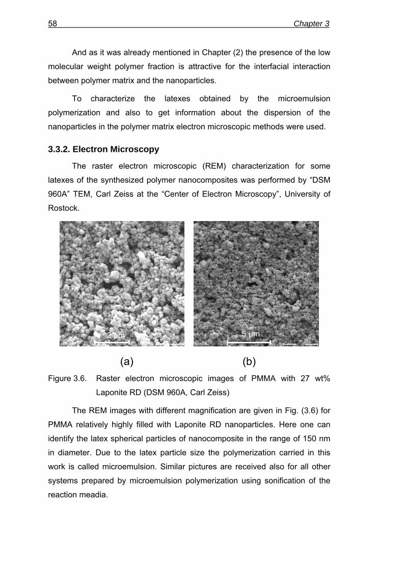
58 Chapter 3
And as it was already mentioned in Chapter (2) the presence of the low
molecular weight polymer fraction is attractive for the interfacial interaction
between polymer matrix and the nanoparticles.
To characterize the latexes obtained by the microemulsion
polymerization and also to get information about the dispersion of the
nanoparticles in the polymer matrix electron microscopic methods were used.
3.3.2. Electron Microscopy
The raster electron microscopic (REM) characterization for some
latexes of the synthesized polymer nanocomposites was performed by “DSM
960A” TEM, Carl Zeiss at the “Center of Electron Microscopy”, University of
Rostock.
(a) (b) Figure 3.6. Raster electron microscopic images of PMMA with 27 wt%
Laponite RD (DSM 960A, Carl Zeiss)
The REM images with different magnification are given in Fig. (3.6) for
PMMA relatively highly filled with Laponite RD nanoparticles. Here one can
identify the latex spherical particles of nanocomposite in the range of 150 nm
in diameter. Due to the latex particle size the polymerization carried in this
work is called microemulsion. Similar pictures are received also for all other
systems prepared by microemulsion polymerization using sonification of the
reaction meadia.
2 μm 5 μm

Experimental 59
The transition electron microscopic (TEM) characterization for some
polymer nanocomposites obtained with intermediate filler content was
performed by “EM 902A” TEM, Carl Zeiss to show the degree of
deagglomeration of nanoparticles and how they are dispersed in the polymer
matrix.
The prepared nanocomposite samples have been pressed at 150°C
under 2 bar excess pressure. Then a thin film of about 10 μm has been cut
from the sample and was embedded into the epoxy resin “Araldit” by Fluka,
Switzerland. The resin was cured at 58 °C in a thermostat for 2-3 days. The
ultrathin cuts (50-100 nm) were obtained on ultramicrotome “Ultrotom III” by
LKB, Sweden and then fixed on the cupper grid and contrasted by uranyl
acetate and plumbum citrate.
Figure 3.7. TEM images of PMMA with 4 wt% SiO2 nanocomposite obtained
by microemulsion polymerization (EM 902 A, Carl Zeiss)
But even by contrasting the samples it was not possible to obtain a
clear picture where one may distinguish the core/shell morphology of
nanoparticles as it is reported for poly(styrene – methylmethacrylate)/SiO2
[99]. The possible reason for that could be the modification of nanoparticles by
oleic acid used for the modification of the nanoparticles in [99] which may be
also considered as additional contrasting. In this work SiO2 nanoparticles have
not been modified in order to obtain two-component systems and
consequently to investigate the interaction between only polymer and
nanopartilces assuming that the SiO2 nanopowder received from Sigma
200 nm50 nm

60 Chapter 3
Aldrich has no surface treatment or some adsorbed substances. Fig. (3.7)
shows that nanoparticles are agglomerated but even in such condition they
still have a great specific surface area.
In recent decade clay nanoparticles have attracted increased attention
due to enhanced functional properties of polymer clay nanocomposites.
Assuming that huge surface area of clay nanoparticles may also result for
composites in a RAF, the PMMA filled with Laponite RD nanocomposites have
been also prepared.
(a) (b)
Figure 3.8. TEM images of PMMA with 11 wt% (a) and 27 wt% (b)
Laponite RD nanocomposite (EM 902 A, Carl Zeiss)
In Fig. (3.8) the TEM images for different Laponite RD loadings of
PMMA nanocomposites are given. One can recognize that at medium filler
contents (11 wt%, Fig. (3.6a)) the clay platelets cover only the surface of
polymer latex particles and with increasing filler content (27 wt%, Fig. (3.8b))
Laponite RD nanoparticles start to penetrate also into the latex particle.
Fig. (3.8) shows that the filler is evenly distributed in the polymer matrix but
these images do not clearly answer the question if the clay nanoparticles are
fully exfoliated in these systems or not.
3.3.3. Small angle X-ray scattering
The SAXS experiments have been performed to clarify if the
Laponite RD clay nanoparticles are exfoliated or not. The measurements have
200 nm 200 nm

Experimental 61
been performed at the Department of Polymer Structures, Leibniz Institute of
Polymer Research, Dresden. The Laponite RD nanopowder has been used as
it was received and also dispersed in water and then dried as described for
sample preparation. The composites have been pressed at 150 °C and dried
as for sample preparation. The analyzing SAXS device was a KRATKY
compact camera (AntonPaar Graz, Austria).
0.1 0.2 0.3 0.4 0.5 0.6 0.7 0.8 0.9 1.0 1.10.1
1
25 10 12345
Nano-powder without drying Nano-powder dried PMMA/11 wt% Laponite RD (28) PMMA/27 wt% Laponite RD (30)I*
s /cp
s*nm
-1
s /nm-1
d(nm) (~1.2 ) (~1.2 ) (~ 2.0) (~ 2.0)
d /nm
Figure 3.9. Common comparison of Lorentz-corrected SAXS-curves
(Ism(s)*s vs. s) for Laponite RD with (red line) and without (blue
line) drying and for PMMA filled with 11 wt% (green line) and
27 wt% (magenta line) Laponite RD
The data shown in Fig. (3.9) were obtained without any treatment like
absorption correction, background correction or desmearing procedures.
Calculation of BRAGG values d from the positions of the scattering maxima
(layer reflections) was performed as follows.
2 d sin Θ = n λ (3.3)
Here 1/d = s is the scattering vector and λ is wave length (Cu-Kα
radiation ≈ 0.154 nm). Fig. (3.9) presents the outcome of the SAXS
experiments performed.
Fig. (3.9) demonstrates that in polymer clay nanocomposites obtained
the nanoparticles are not exfoliated. The comparison of red (nanopowder
without drying) and blue (dried nanopowder) lines allows making a conclusion
that there is no influence of drying on the clay structure. For both of them the

62 Chapter 3
distance between platelets made up about 1.2 nm. Observing the data for
nanocomposites, one sees that even at low clay loadings still not an exfoliated
system has been obtained. The nanoplatelets with about 2 nm interlayer
distance are present. Consequently the intercalated polymer-nanocomposites
have been obtained by microemulsion polymerization of PMMA with Laponite
RD.
3.3.4. Thermogravimetry
To get the content of the nanofiller in the polymer nanocomposites
thermogravimetric measurements for all samples have been performed on a
Labsys, Setaram, instrument at 2 K/min heating rate in the temperature range
from 30 to 650 °C under air. Thermal degradation of PMMA filled with SiO2
and Laponite RD is presented below in Figs. (3.10).
100 200 300 400 500 600-100
-90
-80
-70
-60
-50
-40
-30
-20
-10
0 PMMA pure (1) 4 wt% SiO2 (2) 15 wt% SiO2 (3) 22 wt% SiO2 (4) 30 wt% SiO2 (5) 47 wt% SiO2 (6) 66 wt% SiO2 (7) 73 wt% SiO2 (8) SiO2 pure
Mas
s los
s in
%
Temperature in °C
(a)100 200 300 400 500 600
-100
-90
-80
-70
-60
-50
-40
-30
-20
-10
0
PMMA pure (27) 11 wt% Laponite RD (28) 14 wt% Laponite RD (29) 27 wt% Laponite RD (30) 42 wt% Laponite RD (31) 59 wt% Laponite RD (32) Laponite RD pure
Mas
s los
s in
%
Temperature in °C
(b)
100 200 300 400 500 600-100
-90
-80
-70
-60
-50
-40
-30
-20
-10
0
Mas
s los
s in
%
Temperature in °C
PS pure (42) 9 wt% SiO2 (43) 22 wt% SiO2 (44) 46 wt% SiO2 (46)
(c)
Figure 3.10. Thermal degradation of PMMA SiO2 (a) and Laponite RD (b)
nanocomposites synthesized by microemulsion polymerization
and PS SiO2 (c) nanocomposites synthesized by solution
method (Setaram Labsys, TGA/DSC)

Experimental 63
Thermal behavior of the samples based on PMMA and SiO2 is very
similar for each series. Therefore the data only one of them (with the largest
number of samples) - PMMA with SiO2 by microemulsion polymerization is
shown. Fig. (3.10) shows that polymer nanocomposites obtained in this work
while being filled with SiO2 degrade in one step and those with Laponite RD
obviously in two steps. This can be explained by the modification of clay
nanoparticles which also may interact with polymer matrix in a different way
compared to SiO2. Another observation is that the degradation behavior of
composites is not much influenced with increasing filler content. The shift in
the temperature, when degradation starts, makes up maximum 50 K.
100 200 300 400 500 600 700
-80
-70
-60
-50
-40
-30
-20
-10
0
10
500 550 600 650 700-78
-77
-76
-75
-74
1st run 2nd run 3rd run
Mas
s los
s in
wt%
Temperature in °C
1%+
Figure 3.11. Independent measurements of PMMA with 25 wt% SiO2 (15)
nanocomposite using Setaram Labsys, TGA/DSC instrument
The precision of thermogravimetric measurements is certainly of
importance because deviations in filler content may result in misleading
information of RAF existence. The PMMA filled with 25 wt% of SiO2 (15)
nanocomposite obtained by solution method has been independently
measured three times at the same conditions to check the uncertainty of the
measurements. The inset in Fig. (3.11) shows that the deviation is about ±1%.
Information about the polymer-filler system, its preparation method,
nanoparticles size and the filler content which was received by
thermogravimetric measurements, one can find in Table (2).

64 Chapter 3
Table 2. Nanofiller contents for all samples prepared
N Preparation method Polymer Nanofiller type
Nanofiller dimensions
Nanofiller content, wt%
1 0 2 4 3 15 4 22 5 30 6 47 7 66 8
Microemulsion Polymerization PMMA SiO2 D = 10 nm
73 9 0
10 9 11 35 12
Classical emulsion polymerization
PMMA SiO2 D = 10nm
53 13 0 14 10 15 25 16 40 17
Solution method using PMMA (1)
PMMA SiO2 D = 10 nm
48 18 0 19 9 20 28 21 35 22
Solution method using PMMA from Scientific
Polymer Products PMMA SiO2 D = 10 nm
48 23 0 24 5 25 10 26
Shear mixing using PMMA (1)
PMMA SiO2 D = 10 nm
20 27 0 28 11.4 29 14 30 27 31 42 32
Microemulsion polymerization
PMMA Laponite RD d = 1 nm,
D = 30 nm
59 33 0 34 5 35 10 36 15 37
Shearmixing using PMMA Oroglas,
ARKEMA PMMA Al2O3 D = 30 nm
20 38 0 39 12 40 20 41
Solution method using PBMA from Scientific
Polymer Products PBMA SiO2 D = 10 nm
37 42 0 43 9 44 24 45
Solution method using PS 168N, BASF
PS SiO2 D = 10 nm
41

Experimental 65
The characterization of the polymer nanocomposites obtained by
different preparation methods was performed by the available techniques.
After that the existence of a possible RAF was checked.
3.4. RAF determination
Having the polymer nanocomposites prepared and characterized the
question of RAF existence has to be answered. This information can be
available applying the method described by Wunderlich [157] for
semicrystalline polymers. The calorimetric relaxation strength at the glass
transition Δcp can be considered as a tool for determination of the RAF in
semicrystalline polymers and the immobilized fraction in polymer
nanocomposites too.
Fig. (3.12) represents this method for semicrystalline polycarbonate.
The green line is corresponding to the liquid state of polycarbonate. In the
work that polymer has 23% [165] crystallinity which means that magenta line
should represent specific heat capacity above glass transition for such
crystallinity. But as one can see from Fig. (3.12) this is not the case. The
specific heat capacity and consequently Δcp from the calorimetric
measurement is much smaller than expected from 23% crystallinity.
380 390 400 410 420 430 440 450 460
1.5
1.6
1.7
1.8
1.9
2.0
2.1
2.2
e f
d
a
cpb (χcrystal= 0.23)
cpb (χsolid(Tg) = 0.49)
b - c p solid
c - cp liquid
Spec
ific
heat
cap
acity
in J/
K*g
Temperature in K Figure 3.12. Amorphous and semicrystalline polycarbonates specific heat
capacity as a function of temperature; introduction of RAF, see
text [165]

66 Chapter 3
This can be explained by the formation of RAF which does not
contribute to the step height at glass transition. The estimation of RAF is
shown in the following steps. The mobile amorphous fraction can be estimated
having the step in specific heat capacity of semicrystalline polymer Δcp sc from
the measurement (black line in Fig. (3.12)) and the Δcp a for the amorphous
polymer.
51.0)( =Δ
Δ=
ap
scpgma c
cTχ (3.4)
The RAF can be estimated according Eq. (3.5).
26.0)()(1)( =−−= gcgmagra TTT χχχ (3.5)
The same consideration will be applied to detect the existence of an
immobilized polymer fraction (RAF) in polymer nanocomposites. To apply this
method to the samples obtained one needs reasonable precise heat capacity
data, which are available from StepScan DSC measurements as discussed
above.
3.5. Annealing experiments
In this chapter another method to check the RAF existence is described
which is independent on drawing tangents on the heat capacity curves for the
calorimetric relaxation strength determination. This will help to prove the
results obtained from the Δcp determination.
There is a time-dependence of the supercooled polymers properties,
whereby their physical behavior changes as a function of annealing time at
constant temperature. The annealing of polymers can be understood in terms
of their amorphous structure by reference to a typical schematic enthalpy-
temperature diagram, presented in Fig. (3.13). On cooling from an equilibrium
liquid, the enthalpy departs from equilibrium (for simplicity indicated here as a
linear temperature dependence of the enthalpy) and forms a glass at a critical
temperature called the glass transition temperature, Tg, which depends on
cooling rate. The glassy state is characterized by an excess of enthalpy and
consequently there will be a thermodynamic driving force to reduce the
enthalpy towards equilibrium if the annealing temperature Tannealing is held

Experimental 67
constant after cooling through Tg. This reduction in specific enthalpy for pure
amorphous polymers and nanofilled systems should differ considering an
immobilized fraction. If there is a fraction of amorphous polymer in the
composite which does not contribute to the glass transition, then the enthalpy
relaxation of it will have a deficit in comparison to that of the pure polymer.
This assumption is also valid considering the following
∞Δ=Δ∗Δ HTcp (3.6)
Here ΔH∞ is the difference between starting H0 and equilibrium H∞ enthalpy of
the sample. Enthalpy relaxation ΔH(t) Fig. (3.13) can be presented as
anHHH −=Δ 0 (3.7)
Eq. (3.6) shows that ΔH is somehow related to Δcp but the experiments are in
totally different time scales.
Han
H0
Tannealing
liquid
qTg(q)
T
H
glass
annealing
H∞
Figure 3.13. Schematic enthalpy - temperature diagram showing the change
in enthalpy that occurs on cooling at rate q from the equilibrium
liquid (red curve), and the definition of the rate dependent glass
transition temperature Tg(q) (blue curve). Annealing at
temperature Tannealing reduces the enthalpy from H0 to Han
towards an equilibrium value H∞. The black curve describes the
heating after annealing.
Taking into account the arguments above the annealing experiments
have been performed to check the RAF existence independent from Δcp

68 Chapter 3
determination uncertainties. The temperature-time profile of the annealing
measurements performed is presented below in Fig. (3.14a). First, the sample
is heated up to the maximum temperature much above Tg which is in the case
of PMMA 170 °C. At that temperature any kind of thermal history or
mechanical or thermal stresses are excluded. Then the sample is cooled
down at 10 K/min to the current annealing temperature and annealed for
10 hours. Firstly the annealing time was chosen one hour but as the error bar
for enthalpy relaxation determination procedure was larger than an effect
which could be seen, the time of annealing was extended to ten hours. After
cooling to the minimum temperature the sample is heated up to the maximum
temperature. For excess cp determination, the sample was cooled and without
any annealing heated up again at exactly the same conditions. This heating
curve was used as a baseline for the two-curve heat capacity determination to
get the excess heat capacity data. An example of data treatment for pure
PMMA is given in Fig. (3.14b).
0 20 600 620 640 660 680
40
60
80
100
120
140
160
Tem
pera
ture
in °C
Time in min
tanneal= 600 min
70 80 90 100 110 120 130 140 1508
9
10
11
12
13
14
15
-0.2
0.0
0.2
0.4
0.6
0.8
1.0
PMMA annealed at 105°C Baseline
Temperature in °C
Hea
t flo
w in
mW
, End
o up
Excess specific heat capacity in J/K*g
sample
(a) (b)
Figure 3.14. Heat flow rate and excess specific heat capacity as a function of
sample temperature of PMMA annealed at 105°C for 10 h; red
line – first heating after annealing, blue line – baseline without
annealing, magenta line – excess heat capacity
The red line (Fig. (3.14a,b)) represents the first heating scan of the
sample after annealing. Then the excess specific heat capacity of the sample
was determined in accordance with two-curve determination using the second
heating scan (blue line) as a baseline. The magenta line in Fig. (3.14b) shows

Experimental 69
the outcome of the data treatment described. This was performed for different
annealing temperatures to get the dependence of the enthalpy relaxation on
the annealing temperature for the pure polymer and filled systems.
Quantitative comparison of such data allows drawing the conclusion about the
RAF existence in polymer nanocomposites. Namely, the area under the
excess specific heat capacity is determined by integration between 70 and
140 °C. The obtained data are normalized to the polymer mass to allow a
direct comparison between the pure polymer and the nanocomposites. The
excess heat capacity data for pure PMMA, PS and PBMA and its
nanocomposites filled with SiO2 prepared by solution method are given in
Appendix (A2).

70 Chapter 3

4. RESULTS
4.1. DSC measurements
In Chapter (2) several examples of RAF in semicrystalline polymers and
the discussion about the problems of detection of RAF devitrification are given.
Namely the main difficulty occurs because of the overlapping of melting of the
crystalline fraction, reorganization or reversing melting with the RAF relaxation
processes. That is why it is not possible to clearly recognize which process
begins first – melting of crystals or relaxation of the RAF. Such information is
needed to understand the exact mechanism of the RAF devitrification. In this
work it was tried to simplify the task – to exclude the melting of the crystalline
fraction. The crystalline lamellae have been “replaced” by inorganic
nanoparticles of the similar dimensions which are dispersed in a truly
amorphous polymer matrix, i.e. polymer nanocomposites have been used for
investigations. It is assumed that the RAF is formed also in such systems. In
this work the PMMA, PBMA and PS filled with spherical SiO2 nanoparticles
with ca 10 nm diameter and Laponite RD clay nanoparticles with 1 nm
thickness have been used. Different polymers and nanoparticles have been
chosen to investigate the influence of the polymer and nanofiller structure on
the formation of RAF.
First the existence of RAF in the polymer nanocomposites has to be
checked. Wunderlich [157] has introduced a method of RAF determination for
semicrystalline polymers which is described in Chapter (3). According to that
the step height at the glass transition Δcp can be used for the determination of
the RAF in semicrystalline polymers. This method was first applied to detect a
possible immobilized fraction in polymer nanocomposites.
Next, an example is presented how to apply that method to polymer
nanocomposites. In the Fig. (3.1) the green line corresponds to the heat
capacity of the polymer in the liquid state and the blue line to that of the solid
state of PMMA. The Δcp determination is also graphically shown by vertical
double arrow at the glass transition temperature for the pure polymer.

72 Chapter 4
60 70 80 90 100 110 120 130 140 150 160 1701.3
1.4
1.5
1.6
1.7
1.8
1.9
2.0
2.1
2.2
2.3
cp 3phase
c p 2phase c p solid
PMMA pure (1) PMMA+47% SiO2 (6) 2 phases PMMA+47% SiO
2 (6) 3 phases
Spec
ific
Hea
t Cap
acity
in J/
K*g
sam
ple
Temperature in °C
cp liquid
Tg
Δcp
Figure 4.1. Specific heat capacity of PMMA with 47 wt% SiO2
nanocomposite; straight lines are for solid and liquid states for
the pure polymer (green) and polymer nanocomposite according
to two- (magenta) and three-phase (black) model
Assuming that there is 47 wt% SiO2 for instance in the composite, the
magenta lines correspond to the simple mixing rule of the PMMA and SiO2,
e.g. two phase model of the nanocomposite. If the specific heat capacity of the
sample coincides with the black line which shows smaller step at glass
transition, then the deficit in the Δcp can be explained by the existence of RAF,
e.g. three-phase model of the polymer nanocomposites. According to this
model the nanocomposites consist of nanofiller, mobile amorphous fraction
(MAF) and RAF.
It has to be checked if there is RAF in polymer nanocomposites. In case
there is RAF in composite samples obtained one needs the data from the DSC
measurements for them all. Here below in Fig. (4.2, a-d) the specific heat
capacity as a function of sample temperature for four different
“polymer+nanoparticle” systems is given. The normalized data to the polymer
mass for all the other systems are presented in Appendix (A1).

Results 73
30 40 50 60 70 80 90 100 110 120 130 140 1500.70.80.91.01.11.21.31.41.51.61.71.81.92.02.12.22.3
ATHAS data PS pure (42) 9 wt% SiO2 (43) 24 wt% SiO2 (44) 46 wt% SiO2 (45)
Spec
ific
Hea
t Cap
acity
in J/
K*g
sam
ple
Temperature in °C
(a)SiO2
-40 -20 0 20 40 60 80 100
0.6
0.8
1.0
1.2
1.4
1.6
1.8
2.0
2.2 ATHAS data PBMA pure (38) 12 wt% SiO
2 (39)
20 wt% SiO2 (40) 37 wt% SiO
2 (41)
Spec
ific
Hea
t Cap
acity
in J/
K*g
sam
ple
Temperature in °C
SiO2 (b)
30 40 50 60 70 80 90 100 110 120 130 140 150 160 1700.70.80.91.01.11.21.31.41.51.61.71.81.92.02.12.22.3
ATHAS data PMMA pure (18) 9 wt% SiO
2 (19)
28 wt% SiO2 (20) 35 wt% SiO2 (21) 48 wt% SiO2 (22)
Spec
ific
Hea
t Cap
acity
in J/
K*g
sam
ple
Temperature in °C
SiO2 (c)30 40 50 60 70 80 90 100 110 120 130 140 150 160 170
0.70.80.91.01.11.21.31.41.51.61.71.81.92.02.12.22.3 ATHAS data
PMMA pure (27) PMMA+11 wt% Laponite RD (28) PMMA+14 wt% Laponite RD (29) PMMA+27 wt% Laponite RD (30) PMMA+42 wt% Laponite RD (31) PMMA+59 wt% Laponite RD (32)
Step
Scan
Hea
t Cap
acity
in J/
K*g
sam
ple
Temperature in °C
SiO2 (d)
Figure 4.2. Measured specific heat capacity determined in respect to sample
mass for (a) – PS, (b) – PBMA, (c) – PMMA filled with spherical
SiO2 particles of 10 nm diameter prepared by solution method
and (d) - PMMA filled with Laponite RD nanocomposites
synthesized by microemulsion polymerization
But one has to mention that the specific heat capacity data has been
calculated in respect to the sample mass. This means that during the specific
heat capacity calculation the heat flow rate obtained from the measurements
has been divided by the mass of “polymer + nanofiller”. The specific heat
capacity data for polymer nanocomposites are shifted to lower values with
increasing filler content. The lowering is expected considering the additivity of
heat capacity because SiO2 specific heat capacity is lower than that of
polymers used. But such a shift is not observed for semicrystalline polymers
where the specific heat capacity of the crystalline, the rigid amorphous and not
immobilized fractions are very similar below the glass transition. As for

74 Chapter 4
semicrystalline polymers a slight increase in glass transition temperature was
observed for all nanocomposites after carefully drying at reduced pressure.
0 10 20 30 40 50 60 70-1
0
1
2
3
4
5
6
7
8
PMMA/SiO2 (1-8) PMMA/Laponite (27-32) PS/SiO2 (42-45)
T g -
T g pu
re in
K
Filler content in wt% Figure 4.3. Glass transition temperature of the different nanocomposites as
function of filler content. Half step temperature from StepScan
DSC measuremnts. Tg pure PMMA = 111 °C, Tg pure PS = 99 °C
The glass transition temperature of the nanocomposites was
determined as the half step temperature from the StepScan DSC
measurements. The values are slightly different compared to scan
measurements at 10 K/min because of the different time scale of the
experiment. Glass transition temperature and width of the step in heat capacity
were only little affected by the addition of nanofillers. This is different from
semicrystalline polymers where always a significant increase in glass transition
temperature and a broadening of the transition interval is seen, e.g. [159].
One has also to mention that the cp data for pure polymers should
coincide with ATHAS database data [166] within the uncertainty of DSC
measurements (±1 %) and ATHAS data bank (±5 %). But as it can be seen
from Fig. (4.2b) the PBMA specific heat capacity data are shifted to lower
absolute values in comparison to that of ATHAS database for about 7-8%
which can just be explained by the uncertainties given. For the other pure
polymers the measured curves are in good agreement with the ATHAS
database values.

Results 75
30 40 50 60 70 80 90 100 110 120 130 140 150 160 1701.0
1.2
1.4
1.6
1.8
2.0
2.2 ATHAS data PMMA pure (18) PMMA+35% SiO2 (21) PMMA+48% SiO2 (22)
Spec
ific
Hea
t Cap
acity
in J/
K*g
sam
ple
Temperature in °C
Δcp
Figure 4.4. The determination of the calorimetric relaxation strength at glass
transition for the PMMA SiO2 nanocomposites
The specific heat capacity data given are needed to estimate the
calorimetric relaxation strength at glass transition in order to check if there is a
RAF [157] in polymer nanocomposites obtained or not. As it was already
mentioned one has to draw the tangents outside the glass transition region.
Then the step height at Tg has to be estimated as it is shown in Fig. (4.4)
which is Δcp. The determination of Δcp for PMMA pure and filled with 35 wt%
and 48 wt% SiO2 nanocomposites is presented in Fig. (4.4).
In Fig. (4.4) the tangents drawn in solid and liquid states of specific heat
capacity curves for filled systems appear to have different slopes from that of
the ATHAS database [166] and pure polymer. Moreover the slope change is
larger with increasing filler content. This is discussed next in Chapter (4.2).
4.2. Specific heat capacity correction
For the comparison of the results from calorimetric measurements the
exclusion of the SiO2 contribution to the total heat capacity of the polymer
nanocomposite is needed. Considering the additivity of the heat capacity the
SiO2 contribution should be subtracted which is described below step by step.
In Fig. (4.5) the specific heat capacity dependence on sample temperature for
PMMA nanocomposites is presented as it was measured. As there is a
number of series for different preparation methods, only the data for one of

76 Chapter 4
them are given here as an example and the corrected data to the polymer
mass in Appendix (A1).
30 40 50 60 70 80 90 100 110 120 130 140 150 160 170
0.8
1.0
1.2
1.4
1.6
1.8
2.0
2.2 ATHAS data PMMA pure (18) 9 wt% SiO2 (19) 28 wt% SiO2 (20) 35 wt% SiO2 (21) 48 wt% SiO2 (22) SiO2 lit. data SiO2 dried up to 550°C
Spec
ific
Hea
t Cap
acity
in J/
K*g
sam
ple
Temperature in °C Figure 4.5. Specific heat capacity of polymer fraction as function of
temperature for PMMA SiO2 nanocomposites prepared by
solution method (the measured data)
In Fig. (4.1) the outcome of DSC measurements for PMMA SiO2
nanocomposites prepared by solution method is presented. To check the data
precision the specific heat capacity of PMMA from ATHAS database is also
given [166]. From the graph it is seen that the data for pure polymer does not
coincide with that of ATHAS database. But the difference is within the range of
the precision in absolute values of specific heat capacity which is for these
measurements ± 2 %, see Chapter (3). Moreover in solid state the pure
polymer and ATHAS database curves are parallel which means that the
measurements themselves gave reliable results. The discrepancy between
measured specific heat capacity of pure PMMA and that of ATHAS database
above Tg in liquid state is not known.
The SiO2 specific heat capacity is presented by dotted lines as well. The
dark yellow line corresponds to the literature data [204] for the bulk material
and the navy one is the measured specific heat capacity of SiO2 nanopowder
after drying at 550 °C in DSC in dry nitrogen. It is clearly seen that the
measured data has higher absolute values than that available from the
literature. It can be explained by the contribution of bounded water on the

Results 77
nanoparticles surface due to their great surface area. This indicates the
difficulties with precise cp measurements for systems with large surface areas.
But the nanocomposites were prepared by solution method which is described
in Chapter (3.2) and then dried under reduced pressure at 150 °C which is well
above the Tg of PMMA. Therefore for the subtraction the more reliable data
from the literature was taken because the surface of the nanoparticles is most
probably covered by polymer and the specific heat capacity should not include
a large contribution from water but this is not known in detail.
First step is to determine heat capacity (J/K) of each sample by
multiplication of the specific heat capacity data (J/K*gsample) by the mass of the
sample. Out of this step one gets the heat capacity data as it is shown in Fig.
(4.6).
30 40 50 60 70 80 90 100 110 120 130 140 150 160 1700
5
10
15
20
25
30
35
40
PMMA pure (18) 9 wt% SiO2 (19) 28 wt% SiO2 (20) 35 wt% SiO2 (21) 48 wt% SiO2 (22)
Hea
t Cap
acity
in m
J/K
Temperature in °C
SiO2
Figure 4.6. Heat capacity of PMMA SiO2 nanocomposites prepared by
solution method (the heat capacity for the SiO2 fraction of each
sample is also given)
The contribution of the SiO2 fraction of each sample is shown in Fig. (4.6) in
the similar color as used for the corresponding sample. The heat capacities for
the polymer in each polymer nanocomposite after subtraction are shown in
Fig. (4.7).

78 Chapter 4
30 40 50 60 70 80 90 100 110 120 130 140 150 160 1700
5
10
15
20
25
30
35
40
PMMA pure (18) 9 wt% SiO2 (19) 28 wt% SiO2 (20) 35 wt% SiO2 (21) 48 wt% SiO2 (22)
Hea
t Cap
acity
in m
J/K
Temperature in °C Figure 4.7. Heat capacity of the polymer of PMMA SiO2 nanocomposites
prepared by solution method
The heat capacity data shown Fig. (4.7) could be compared with each
other only as specific heat capacity data after the individual division by the
polymer masses for each sample.
30 40 50 60 70 80 90 100 110 120 130 140 150 160 1701.0
1.2
1.4
1.6
1.8
2.0
2.2 ATHAS data PMMA pure (18) 9 wt% SiO
2 (19)
28 wt% SiO2 (20)
35 wt% SiO2 (21) 48 wt% SiO
2 (22)
Spec
ific
Hea
t Cap
acity
in J/
K*g
poly
mer
Temperature in °C Figure 4.8. Specific heat capacity of the polymer fraction as function of
temperature for PMMA SiO2 nanocomposites prepared by
solution method
From the division we get the specific heat capacity in J/K*gpolymer. It is
expected that the curves coinciding in the solid state with ATHAS database
data or at least with the pure PMMA due to the same degrees of freedom,
which is not the case as shown in Fig. (4.8). What can be seen is that the

Results 79
specific heat capacity data for the filled systems lie higher than that of the pure
polymer and ATHAS database. This means that by the subtraction described
above the contribution of the SiO2 is overcompensated. But it is known from
Chapter (3.3) that the thermogravimetric measurements have approximately
± 1% uncertainty. Taking this into account and assuming that the determined
filler content is not correct, the filler content was varied within the uncertainty.
This way the heat capacity data for any filler loading could be shifted to that of
the pure polymer by changing the filler content within 1-2% and performing the
subtraction steps as described. Consequently one can rely on the results
obtained from the DSC measurements only within the uncertainty of heat
capacity and filler content.
There may be another reason for the discrepancy too. The specific heat
capacity of the SiO2 nanopowder is not known precisely. Fig. (4.9) represents
the outcome of the subtraction procedure using the measured SiO2 data
(dotted line). Comparing this graph with that shown in Fig. (4.5) one can see
that there is nearly no difference in absolute values before and after
subtraction. And the final values differ from the ATHAS database values by up
to 25% and cannot be explained by uncertainty of neither thermogravimetric
nor DSC measurements. This indicates that the cp measurement of the SiO2
nanopowder is superimposed by adsorbed water heat capacity and water
desorption.
As it was already mentioned, in solid state the polymer cp data for each
sample should coincide with that of the pure polymer due to the similar degree
of freedom. And the deviations in cp are the result of the influence of
measurement precision and adsorbed water. In order to allow a direct
comparison of the specific heat capacity, the curves (Fig. (4.8)) were finally
shifted to the ATHAS data bank value at 60 °C. The result is shown in
Fig. (4.10).

80 Chapter 4
30 40 50 60 70 80 90 100 110 120 130 140 150 160 170
0.8
1.0
1.2
1.4
1.6
1.8
2.0
2.2 ATHAS data PMMA pure (18) 9 wt% SiO2 (19) 28 wt% SiO2 (20) 35 wt% SiO2 (21) 48 wt% SiO2 (22)
Spec
ific
Hea
t Cap
acity
in J/
K*g
poly
mer
Temperature in °C
SiO2
Figure 4.9. Specific heat capacity of polymer fraction as function of
temperature for PMMA SiO2 nanocomposites prepared by
solution method (the measured cp of SiO2 nanopowder was used
for the subtraction)
30 40 50 60 70 80 90 100 110 120 130 140 150 160 170
1.2
1.4
1.6
1.8
2.0
2.2 ATHAS data PMMA pure (18) 9 wt% SiO2 (19) 28 wt% SiO2 (20) 35 wt% SiO2 (21) 48 wt% SiO2 (22)
Spec
ific
Hea
t Cap
acity
in J/
K*g
poly
mer
Temperature in °C Figure 4.10. Specific heat capacity as a function of sample temperature for
PMMA SiO2 nanocomposites prepared by solution method
(corrected to the polymer mass by SiO2 contribution subtraction
and vertically shifted to ATHAS data [166] at 60 °C)
In Fig. (4.10) it is now clearly visible that the relaxation strength at glass
transition for different filler loadings is not the same. The higher the filler
content, the lower is the step height at glass transition even the data are
corrected for the filler content and presented in respect to polymer mass. This

Results 81
deficit in Δcp means that there is some RAF. Therefore the results obtained so
far can be explained by introduction of a RAF in the PMMA SiO2 and
Laponite RD nanocomposites (see Appendix (A1)).
As the cp of SiO2 has linear temperature dependence in the temperature
range of interest, the cp data of the samples may be also corrected to that of
the polymer by shift and rotation of the originally measured curves. Again
assuming that in solid state the polymer cp should be the same for all samples
the originally measured data was simply recalculated to that of the polymer
fraction for each loading and then by shifting and rotating fitted to the ATHAS
database data in the solid state in the temperature range of 30 – 80 °C. It is
interesting to check if there is significant difference between the polymer cp
obtained by the SiO2 contribution subtraction and by such simple manipulation.
30 40 50 60 70 80 90 100 110 120 130 140 150 160 170
1.2
1.4
1.6
1.8
2.0
2.2
1.4
1.6
1.8
2.0
2.2
2.4
2.6
PMMA/48 wt% SiO2
SiO2 subtracted PMMA/48 wt% SiO2
not corrected
ATHAS data PMMA pure (18) 9 wt% SiO
2 (19)
28 wt% SiO2 (20)
35 wt% SiO2 (21)
48 wt% SiO2 (22)
Spec
ific
Hea
t Cap
acity
in J/
K*g
poly
mer
Temperature in °C Figure 4.11. Specific heat capacity as a function of sample temperature
PMMA SiO2 nanocomposites prepared by solution method
(recalculated to the polymer mass and fitted to ATHAS data [166]
in solid state)
For the direct comparison the specific heat capacity of PMMA / 48 wt%
SiO2 was corrected to the polymer mass as shown in Fig. (4.10) (black dotted
line, Fig. (4.11)). It is seen that there is nearly no discrepancy between the
data corrected by the subtraction of bulk SiO2 cp (black dotted line) and that of
just shifted and rotated (magenta dotted line). Uncertainty has been estimated

82 Chapter 4
as 1 - 2%. As one can see even the shape of glass transition, as well as the
slopes in liquid state are similar in both cases (the dotted lines).
The data for PS (Fig. (4.12)) as well as all the other samples
(Appendix (A1)) were also corrected in the similar way. The PS filled with SiO2
nanocomposites do not exhibit RAF as it is seen from the Fig. (4.12). The data
for each nanofiller loading coincides with that of ATHAS database after
recalculation to the polymer mass. The only difficulty to draw such a
conclusion comes from the specific heat capacity curve for highest filler
content (cyan, Fig. (4.12)). The step in polymer cp at glass transition for that
sample is smaller that those for the other samples. This may be explained by
the influence of the large quantity of adsorbed water on the free (in case of no
interaction) surface of nanoparticles but not known exactly.
30 40 50 60 70 80 90 100 110 120 130 140 150
1,2
1,4
1,6
1,8
2,0
2,2 ATHAS data PS pure (42) PS+9 wt% SiO2 (43) PS+24 wt% SiO2 (44) PS+46 wt% SiO2 (45)
Spec
ific
Hea
t Cap
acity
in J/
K*g
sam
ple
Temperature in °C Figure 4.12. Specific heat capacity as a function of sample temperature PS
SiO2 nanocomposites prepared by solution method (recalculated
to the polymer mass and fitted to ATHAS data [166] in solid
state)
In Chapter (4.2) it was mentioned that large scatter in Δcp data for
PBMA filled with SiO2 nanocomposites is a result of wide glass transition
temperature interval which makes it difficult to draw the tangents to the liquid
and solid states of the polymer cp data. This might be solved by the extension
of the measurement temperature range but was not possible in solid state due
to the instrument limitation (-50 °C) and polymer degradation in liquid state.

Results 83
Anyway for this system the cp data of nanocomposites were also divided by
polymer fraction, shifted and rotated to that of the pure PBMA to observe at
least qualitatively the thermal behavior of the polymer fraction in
nanocomposites at glass transition.
-40 -20 0 20 40 60 80 1000.8
1.0
1.2
1.4
1.6
1.8
2.0
1.2
1.4
1.6
1.8
2.0
2.2
2.4 ATHAS data PBMA pure (38) 12 wt% SiO2 (39) 20 wt% SiO2 (40) 37 wt% SiO2 (41)
Spec
ific
Hea
t Cap
acity
in J/
K*g
poly
mer
Temperature in °C
Δcp
Figure 4.13. Specific heat capacity as a function of sample temperature
PBMA SiO2 nanocomposites prepared by solution method
(recalculated to the polymer mass and fitted to ATHAS data [166]
in solid state)
In Fig. (4.13) it is clearly seen that the cp data for filled systems and
pure PBMA are very much identical after the correction described. This means
that there is not a significant amount of RAF in PBMA filled with SiO2
nanocomposites. Such a disagreement between this observation and the Δcp
values may be explained by the example of Δcp determination varying the
slope of the tangents drawn which is presented in Fig. (4.13) with respect to
the right scale. The magenta tangents are drawn following the slopes in solid
and liquid states of the measured cp data for PBMA filled with 37 wt% of SiO2.
The navy tangents are parallel to those of ATHAS database data. It is obvious
that by small variation of the tangent slope determined Δcp data might have up
to 30% uncertainty. Therefore the method of RAF recognition in polymer
nanocomposites based on Δcp determination is not applicable for all systems
and one needs to check the RAF existence in polymer nanocomposites by
another independent experiment described in Chapter (4.4).

84 Chapter 4
But the purpose of this work is to quantify the immobilized polymer
fraction in the polymer nanocomposites showing RAF which is, according to
[157] available from the measured cp data.
4.3. RAF determination
Following the idea of RAF determination by [25, 36] Δcp and Δcp pure are
the calorimetric relaxation strength at glass transition of the nanocomposite
and pure polymer, respectively. An immobilized or rigid amorphous fraction
can be determined from heat capacity according Eq. (3.5) replacing the
crystalline by the nanoparticle fraction [25, 36].
RAF = 1 – filler content - Δcp/ Δcp pure (4.1)
In Fig. (4.14) the Δcp data for PMMA filled with SiO2 nanoparticles
prepared by microemulsion polymerization are given. The normalization of the
data to the polymer mass is also needed to be able to compare the values for
different polymer nanocomposites in one graph directly. Depending on the
preparation method Δcp of the pure polymer for each series may differ.
In Fig. (4.14) according Eq. (4.1) the diagonal represents the case when
no RAF is present. In other words a two phase system (filler + polymer) is
present, which is expected if there is no interfacial immobilization. The steeper
red line is a guide for eye to show the decrease of the Δcp data for PMMA SiO2
nanocomposites by microemulsion polymerization. The upper arrow at 53 wt%
filler corresponds to the filler fraction. The lowest indicates the mobile
amorphous fraction (MAF) contributing to the calorimetric relaxation strength at
glass transition.

Results 85
0 10 20 30 40 50 60 70 80 90 1000,0
0,1
0,2
0,3
0,4
0,5
0,6
0,7
0,8
0,9
1,0
MAF
SiO2
Microemulsion polymerization (1-8)
Δcp
sam
ple /
Δcp p
ure
Filler content in wt%
RAF
Figure 4.14. Normalized calorimetric relaxation strength as a function of
nanofiller content for PMMA filled with SiO2 nanocomposites
prepared by microemulsion polymerization; the vertical magenta
double arrow indicates the amount of RAF at 53% filler (green
double arrow) and the blue one corresponds to MAF
The difference between the measured values and the diagonal (middle
arrow) represents the immobilized (rigid) fraction (RAF) which can be
calculated according Eq. (4.1). It corresponds to the mobile amorphous
fraction contributing to the relaxation strength at Tg.
In Fig. (4.15a) the data for all preparation methods are given. The points
for each preparation method lie nearly on the same red line as for
microemulsion polymerization. One can see that unexpectedly the interaction
strength between PMMA matrix and nanofiller surface, which should define the
amount of RAF, does not depend much on the preparation technique. As next
the results for PMMA filled with Laponite RD and aluminum oxide (Al2O3, ca 30
nm in diameter) nanocomposites are presented in Fig. (4.15b).

86 Chapter 4
0 10 20 30 40 50 60 70 80 90 1000,0
0,1
0,2
0,3
0,4
0,5
0,6
0,7
0,8
0,9
1,0 Microemulsion p-n (1-8) Sol-n m-d with polymer (13-17) S-n m-d with standard (18-22) Classical emulsion pol-n (9-12) Shearmixing (23-26)
Δcp
sam
ple /
Δc p p
ure
Filler content in wt%
RAF
(a)0 10 20 30 40 50 60 70 80 90 100
0,0
0,1
0,2
0,3
0,4
0,5
0,6
0,7
0,8
0,9
1,0
PMMA/Laponite RD (27-32) PMMA/Al2O3 (33-37)
Δc p
sam
ple /
Δc p p
ure
Filler content in wt%
RAF
(b)
Figure 4.15. Normalized calorimetric relaxation strength as a function of
(a) nanofiller content for PMMA filled with SiO2 nanocomposites
prepared by microemulsion polymerization (squares), solution
method using synthesized PMMA (circles), solution method with
PMMA from Scientific Polymer Products (triangles), classical
emulsion polymerization (stars), shear mixing (diamonds); the
vertical double arrow indicates the amount of RAF at 53% filler
(b) PMMA with Laponite RD (green squares) and Al2O3 (cyan
squares) nanocomposites
Here the green line is a guide for eye showing the decrease of the
relaxation strength data for PMMA Laponite RD nanocomposites and is
steeper than that of PMMA SiO2 samples. On the contrary to that the diagonal
fits to the points for PMMA Al2O3 nanocomposites. From the description of the
materials used (Chapter 3) it is known that Laponite RD nanoparticles have
platelet-like form with 1 nm thickness. This means that they have larger
effective surface area than spherical SiO2 nanoparticles with 10 nm diameter.
Therefore it is expected that at the same nanofiller content exfoliated or
intercalated Laponite RD particles immobilize larger quantity of the polymer
than SiO2 what can be recognized in Fig. (4.15b). Even the glass transition
disappears (Δcp = 0) at about 50 wt% for the Laponite RD filler (Fig. 4.2d), e.g.
the whole polymer is immobilized by the nanoparticles. The Δcp data of PMMA
Al2O3 nanocomposites shows that there is no RAF detected. The calorimetric
relaxation strength data for PBMA and PS filled with SiO2 is presented in
Fig. (4.16).

Results 87
0 10 20 30 40 50 60 70 80 90 1000,0
0,1
0,2
0,3
0,4
0,5
0,6
0,7
0,8
0,9
1,0
Solution method PBMA / SiO2
(38-41)Δc
p sa
mpl
e / Δc
p pur
e
Filler content in wt%
(a)0 10 20 30 40 50 60 70 80 90 100
0,0
0,1
0,2
0,3
0,4
0,5
0,6
0,7
0,8
0,9
1,0
Solution method PS168N / SiO2
(42-45)
Δc p
sam
ple /
Δcp p
ure
Filler content in wt%
(b)
Figure 4.16. Normalized calorimetric relaxation strength as a function of
nanofiller content for (a) - PBMA and (b) – PS with SiO2
nanocomposites
Fig. (4.16a) demonstrates the extremely large uncertainty of the data for
PBMA SiO2. The magenta line might show the RAF existence following the
points but taking into consideration the error bar no conclusion is drawn for
PBMA based systems. The discrepancy in data can be explained by the shape
of glass transition for PBMA. In Fig. (4.2b) one can see that the glass transition
has larger temperature interval than for PMMA and PS. This causes difficulties
to draw the tangents during Δcp determination. Fig. (4.16b) shows the Δcp data
for PS SiO2 system. The points lie close to the diagonal, which according
Eq. (4.1) represents the case when no RAF is present. In other words a two
phase system (filler + polymer) is present, which is expected if there is no
interfacial immobilization.
Having Δcp data for all systems observed the RAF content has been
estimated for all the systems prepared by means of Eq. (4.1). The results
obtained and normalized to the whole polymer fraction in composites are given
in Fig. (4.17) as function of the filler content. The red and green lines present
the data for PMMA SiO2 and Laponite RD nanocomposites respectively.

88 Chapter 4
0 10 20 30 40 50 60 70 80
0,0
0,1
0,2
0,3
0,4
0,5
0,6
0,7
0,8
0,9
1,0 PMMA/SiO2 (1-8) PMMA/Laponite RD (27-32) PS/SiO
2 (42-45)
PBMA/SiO2 (38-41)
RA
F / P
olym
er fr
actio
n
Filler content in wt% Figure 4.17. Normalized RAF as a function of filler content for (red) – PMMA
with SiO2, (green) - PMMA with Laponite RD, (blue) – PS with
SiO2 and (magenta) – PBMA with SiO2 nanocomposites
The blue and magenta lines correspond to the data for PS and PBMA
SiO2 nanocomposites respectively. As it can be seen from Fig. (4.8) the RAF
seems to be linearly dependent on the nanofiller content due to most likely
agglomeration of the nanoparticles. For Laponite RD filled PMMA
nanocomposites the RAF even saturated at highest filler concentration
(59 wt%).
The situation for the PS and especially PBMA composite samples is not
clear due to not well defined tangent construction. In these cases the
determination of Δcp for RAF estimation is uncertain. Molecular mobility at and
below the glass transition can be tested by annealing experiments too, see
[205] for a review. If a fraction of the amorphous polymer in the
nanocomposites is immobilized it is expected that enthalpy relaxation below
glass transition is reduced too [206, 207]. To check if this provides more
definite results regarding RAF the following annealing experiments were
performed.
4.4. Annealing experiments
As follows from the previous chapter at this step the results obtained
from Δcp estimation are checked by another method, independent on tangent
construction – annealing experiments. If a fraction of the amorphous polymer

Results 89
in the nanocomposites is immobilized it is expected that enthalpy relaxation
below glass transition is reduced too [206, 207]. To check if this provides more
definite results regarding RAF the following annealing experiments were
performed. Following the idea described in Chapter (3.5) it is shown that in this
work during the excess specific heat capacity determination from the
annealing experiments not an empty pan was used as a baseline but the
second heating scan without annealing of the same sample. This allows
comparing the behavior of only the polymer and any influence of adsorbed
water etc may be neglected.
As it is described in Chapter (3.5) the samples were heated well above
the Tg to erase the previous thermal history. Then after cooling at 10 K/min to
the annealing temperature they were annealed for 10 hours. For the detection
of the enthalpy change due to the annealing, the composite samples were
cooled and reheated again.
50 60 70 80 90 100 110 120 130 140-0.2
-0.1
0.0
0.1
0.2
0.3
0.4
0.5
0.6
0.7
0.8
0.9
1.0
Ta = 60°C
Ta = 80°C
Ta = 90°C
Exce
ss sp
ecifi
c he
at c
apac
ity in
J/K
*gsa
mpl
e
Temperature in °C
Ta = 95°C
Figure 4.18. Excess specific heat capacity after annealing at different
temperatures versus temperature for pure PS (42); the annealing
time is 10 h, sample mass 17 mg
The typical annealing peak is seen in the first heating, which is not
present in the next heating without annealing (Fig. (3.14)). The difference of
both curves yields excess heat capacity as shown in Fig. (4.18) for PS. The
data for PMMA and PBMA filled with SiO2 nanocomposites are presented in
Appendix (A2). Integration from 70 to 140 °C finally gives the specific enthalpy

90 Chapter 4
change ΔH during annealing. To allow a direct comparison the specific
enthalpy change was normalized to the polymer fraction of the
nanocomposites. Because of the small shift in glass transition temperature
results are plotted versus Tannealing - Tg. Here the peak position shifts from
higher to lower temperatures with decreasing annealing temperature.
-100 -80 -60 -40 -20 0 20-0,4
-0,3
-0,2
-0,1
0,0
0,1
0,2
0,3
0,4
0,5
0,6
0,7
0,8
PMMA pure (1) PMMA+15% SiO2 (3)
Enth
alpy
in J/
g poly
mer
Tanneal-Tg in K
(a)
-70 -60 -50 -40 -30 -20 -10 0 10
-0,2
-0,1
0,0
0,1
0,2
0,3
0,4
0,5
0,6
0,7
0,8
0,9
PBMA pure (38) PBMA+20% SiO2 (40)
Enth
alpy
in J/
g poly
mer
Tanneal-Tg in K
(b)
-35 -30 -25 -20 -15 -10 -5 0-0,2
0,0
0,2
0,4
0,6
0,8
1,0
1,2 PS pure (42) PS+24% SiO2 (44)
Enth
alpy
in J/
g poly
mer
Tanneal.-Tg in K
(c)
Figure 4.19. Enthalpy change (J/gpolymer) during annealing for 1 h as function
of the annealing temperature for (a) – PMMA, (b) – PBMA, (c) -
PS and its SiO2 nanocomposites; Tg PMMA = 111 °C,
Tg composite = 113 °C; Tg PBMA = 30 °C, Tg composite = 31 °C;
Tg PS = 99 °C, Tg composite = 103 °C
The area under the peak first increases and, after some maximum,
decreases with increasing annealing temperature. This is better seen in
Fig. (4.19) where the enthalpy change (J/gpolymer) during annealing for 1 h as
function of the annealing temperature is shown. The maximum for the samples
is in the glass transition region, just 5 – 10 K below Tg, as expected. The error
bars in Fig. (4.19) indicate that the effect observed is smaller or in the same

Results 91
range as the uncertainty of such measurements. Therefore the annealing time
has been extended to 10 h in order to increase the area under the peak in
excess cp data.
The enthalpies determined from the annealing peaks (Tannealing = 10 h)
for pure PS and its nanocomposite with 24 wt% of SiO2 are represented in the
Fig. (4.20). For this system no difference in the enthalpy relaxation for the pure
polymer and the nanocomposite is detected as shown in Fig. (4.20).
-120-110-100-90 -80 -70 -60 -50 -40 -30 -20 -10 0 10 20 30 40 50
-0,2
0,0
0,2
0,4
0,6
0,8
1,0
1,2
1,4 PS pure (42) 24 wt% SiO2 (44)
Enth
alpy
in J/
g poly
mer
Tanneal-Tg in K Figure 4.20. Enthalpy change (J/gpolymer) during annealing for 10 h as function
of the annealing temperature for PS and PS SiO2
nanocomposite; Tg PS = 99 °C, Tg composite = 103 °C

92 Chapter 4
-80 -60 -40 -20 0 20 40
-0,2
0,0
0,2
0,4
0,6
0,8
1,0
1,2
1,4
PBMA pure (38) PBMA+20% SiO2 (40)
Ent
halp
y in
J/g po
lym
er
Tanneal-Tg in K Figure 4.21. Enthalpy change (J/gpolymer) during annealing for 10 h as function
of the annealing temperature for PBMA and PBMA with SiO2
nanocomposite; Tg PMMA = 30 °C, Tg composite = 31 °C
As expected from the dewetting properties of PS on silica surface pure PS and
the polymer fraction in the PS with 24 wt% SiO2 behave in the same way - the
data for them both coincide within the error limit of ±0.1 J/g.
Such a discrepancy may appear as a result of the error coming from the
thermogravimetric measurements, see Chapter (3.3). Fig. (4.21) demonstrates
the same situation for pure PBMA and the composite with 20 wt% SiO2.
-120-110-100 -90 -80 -70 -60 -50 -40 -30 -20 -10 0 10 20 30
-0,2
0,0
0,2
0,4
0,6
0,8
1,0
1,2
1,4 PMMA pure (18) PMMA+35% SiO2 (21)
Enth
alpy
in J/
g poly
mer
Tanneal-Tg in K Figure 4.22. Enthalpy change (J/gpolymer) during annealing for 10 h as function
of the annealing temperature for PMMA and PMMA with SiO2
nanocomposite; Tg PMMA = 111 °C, Tg composite = 113 °C
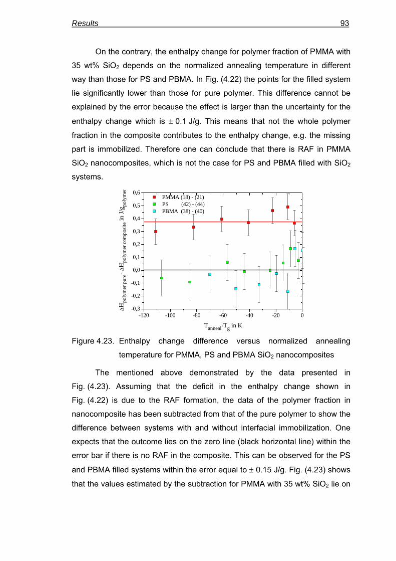
Results 93
On the contrary, the enthalpy change for polymer fraction of PMMA with
35 wt% SiO2 depends on the normalized annealing temperature in different
way than those for PS and PBMA. In Fig. (4.22) the points for the filled system
lie significantly lower than those for pure polymer. This difference cannot be
explained by the error because the effect is larger than the uncertainty for the
enthalpy change which is ± 0.1 J/g. This means that not the whole polymer
fraction in the composite contributes to the enthalpy change, e.g. the missing
part is immobilized. Therefore one can conclude that there is RAF in PMMA
SiO2 nanocomposites, which is not the case for PS and PBMA filled with SiO2
systems.
-120 -100 -80 -60 -40 -20 0-0,3
-0,2
-0,1
0,0
0,1
0,2
0,3
0,4
0,5
0,6 PMMA (18) - (21) PS (42) - (44) PBMA (38) - (40)
ΔHpo
lym
er p
ure- Δ
Hpo
lym
er c
ompo
site
in J/
g poly
mer
Tanneal-Tg in K Figure 4.23. Enthalpy change difference versus normalized annealing
temperature for PMMA, PS and PBMA SiO2 nanocomposites
The mentioned above demonstrated by the data presented in
Fig. (4.23). Assuming that the deficit in the enthalpy change shown in
Fig. (4.22) is due to the RAF formation, the data of the polymer fraction in
nanocomposite has been subtracted from that of the pure polymer to show the
difference between systems with and without interfacial immobilization. One
expects that the outcome lies on the zero line (black horizontal line) within the
error bar if there is no RAF in the composite. This can be observed for the PS
and PBMA filled systems within the error equal to ± 0.15 J/g. Fig. (4.23) shows
that the values estimated by the subtraction for PMMA with 35 wt% SiO2 lie on
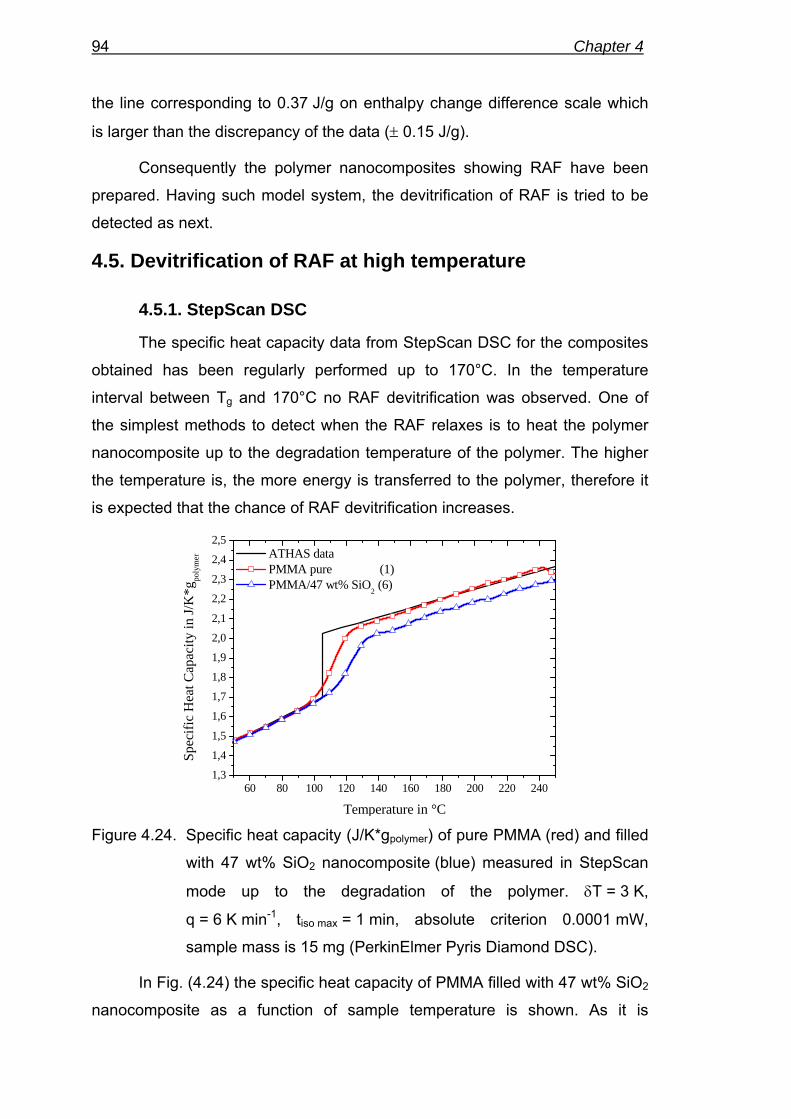
94 Chapter 4
the line corresponding to 0.37 J/g on enthalpy change difference scale which
is larger than the discrepancy of the data (± 0.15 J/g).
Consequently the polymer nanocomposites showing RAF have been
prepared. Having such model system, the devitrification of RAF is tried to be
detected as next.
4.5. Devitrification of RAF at high temperature
4.5.1. StepScan DSC
The specific heat capacity data from StepScan DSC for the composites
obtained has been regularly performed up to 170°C. In the temperature
interval between Tg and 170°C no RAF devitrification was observed. One of
the simplest methods to detect when the RAF relaxes is to heat the polymer
nanocomposite up to the degradation temperature of the polymer. The higher
the temperature is, the more energy is transferred to the polymer, therefore it
is expected that the chance of RAF devitrification increases.
60 80 100 120 140 160 180 200 220 2401,3
1,4
1,5
1,6
1,7
1,8
1,9
2,0
2,1
2,2
2,3
2,4
2,5 ATHAS data PMMA pure (1) PMMA/47 wt% SiO2 (6)
Spec
ific
Hea
t Cap
acity
in J/
K*g
poly
mer
Temperature in °C Figure 4.24. Specific heat capacity (J/K*gpolymer) of pure PMMA (red) and filled
with 47 wt% SiO2 nanocomposite (blue) measured in StepScan
mode up to the degradation of the polymer. δT = 3 K,
q = 6 K min-1, tiso max = 1 min, absolute criterion 0.0001 mW,
sample mass is 15 mg (PerkinElmer Pyris Diamond DSC).
In Fig. (4.24) the specific heat capacity of PMMA filled with 47 wt% SiO2
nanocomposite as a function of sample temperature is shown. As it is

Results 95
mentioned in Chapter (1) the RAF devitrification is expected to appear as a
second glass transition but as it is clear from the Fig. (4.24), there is no
steplike transition observed up to 230°C when the polymer starts to degrade.
4.5.2. High rate DSC
Influence of degradation on the heat capacity determination can be
reduced by using high heating rates. Using high rates up to 400 K/min the
polymer does not degrade even up to nearly 350 °C. And as the RAF
relaxation is expected to appear at the temperatures higher than conventional
Tg, it was supposed that this would help to detect the devitrification of RAF.
50 100 150 200 250 300 350
1.4
1.6
1.8
2.0
2.2
2.4
2.6 ATHAS data PMMA pure (1) PMMA+47 wt% SiO2 (6)
Spec
ific
heat
cap
acity
in J/
K*g
poly
mer
Temperature in °C Figure 4.25. Hyper DSC [208] measurements at 400 K/min heating rate, mass
of each sample is 0.9 mg
But as it is seen from the Fig. (4.25) there is no any second glass
transition up to nearly 350 °C. This means that the interaction between
polymer matrix and nanoparticles is so strong that heating even up to such
high temperatures is not enough to devitrify RAF.
4.6. Plasticization experiments
As the high rate DSC was not enough to detect the RAF devitrification
calorimetrically, another method – plasticization of the polymer was used. The
plasticizer was added to lower the Tg hoping that the devitrification of the
immobilized polymer fraction will be also lowered. The idea is following. The
polymers we used degrade in the temperature range of 200-250 °C at low

96 Chapter 4
heating rates. This limits the measurement interval to between the Tg of MAF
and degradation temperature of the polymer. What one can do is to shift the Tg
of the MAF to lower temperatures which will enlarge that interval. So the
chance to devitrify the RAF is higher than without plasticizer addition. Of
course, this will work only in case if RAF is plasticized as well. For these
experiments the chloroform as plasticizing agent was used.
In Fig. (4.26) the specific heat capacity data from the pure PMMA and
PMMA with 47 wt% of SiO2 nanocomposites plasticized by different amounts
of chloroform is given.
-40 -20 0 20 40 60 80 100 120 140 160
0.6
0.8
1.0
1.2
1.4
1.6
1.8
2.0
2.2
2.4
2.6
2.8
3.0
32 wt% Chloroform
PMMA pure (1) PMMA with 47% SiO2 (6) ATHAS data
Spec
ific
Hea
t Cap
acity
in J/
K*g
dry
sam
ple
Temperature in °C
dry samples
32 wt% Chloroform
Figure 4.26. Specific heat capacity of the plasticized samples as a function of
sample temperature for PMMA pure (green curves) and
PMMA / 47 wt% SiO2, mass of dry samples is 15 mg (pure
PMMA) and 20 mg (PMMA / 47 wt% SiO2), the maximum
concentration of chloroform is 46 wt% in respect to polymer
The weight percentage is given in relation to the polymer mass. As one
can see the Tg of both pure PMMA and composite at 32 wt% chloroform is
nearly the same. This may mean that the organic solvent plasticizes the whole
polymer in composite, even immobilized fraction. But one has to be careful
while comparing different samples.
As it was mentioned above the Tg of RAF will be lowered only in case if
the solvent penetrates into the RAF. This can be checked by using the Fox
equation (Eq. (4.2)) [209] for two-component systems.

Results 97
solvg
solv
polg
pol
g TTTωω
+=1 (4.2)
Here Tg, Tg pol and Tg solv are the glass transition temperatures of
plasticized system, polymer and solvent respectively, ωpol and ωsolv are weight
fractions of the polymer and solvent respectively. For comparison of the data
obtained so called “calibration curve” is shown in Fig. (4.27). In other words, it
is the Tg of the pure polymer as a function of solvent concentration which
follows Fox equation. The same dependence was evaluated from the Fig.
(4.26) for the filled system and plotted with the calibration curve together. If the
solvent lowers the Tg of the polymer in both samples in the same way, this will
mean that it plasticizes the RAF also. And vice versa, if the data for the
composite do not follow the calibration curve, it will indicate that RAF is not
plasticized. Tg for pure polymer and the composite is not the same, therefore in
Fig. (4.27) the difference between dry sample Tg and that of the plasticized is
plotted versus solvent concentration.
0,0 0,1 0,2 0,3 0,4 0,5 0,6 0,7 0,8 0,9 1,0-200
-180
-160
-140
-120
-100
-80
-60
-40
-20
0 PMMA pure (1) PMMA with 47% SiO2 (6)
with respect to whole polymer with respect to MAF
Fox equation fit
T g pl
astic
ized
-Tg
dry in
K
Solvent content in mass fraction Figure 4.27. Normalized glass transition depending on the plasticizer
concentration, Tg dry PMMA = 111 °C, Tg dry composite = 118 °C
From this graph one can see that in comparison to the pure polymer,
the polymer fraction of the composite is completely plasticized. While solvent
concentration is estimated in respect to the whole polymer mass the data for
the filled system are lying on the same line as the data from the pure PMMA
within the error limit. This means that chloroform penetrates into either MAF or

98 Chapter 4
RAF in polymer nanocomposites obtained. But the devitrification of the RAF is
not observed from the data presented (Fig. (4.27)). There are two possible
explanations for that. First is that the RAF devitrification is spread over the
large temperature interval from the MAF Tg up to the degradation of the
polymer and by the calorimetric methods used during this work it is not
possible to detect it. The second is that the devitrification of RAF in polymer
nanocomposites does not occur before degradation of polymer.

5. DISCUSSION
Interaction at the filler polymer interface is considered to be important
for the behavior of polymer nanocomposites. Following the work of Lipatov
and Privalko [25, 36] the fraction of immobilized polymer (RAF) was quantified
for PMMA, PBMA and PS SiO2 and PMMA Laponite RD nanocomposites. For
the polymer fraction of the nanocomposites Eq. (4.1) can be rewritten for the
immobilized fraction of the polymer RAFpolymer [25, 36]
RAFpolymer = 1 – Δcp polymer/ Δcp pure (5.1)
From Figs. (4.11, 4.12) and Fig. (A1.5) the step height in specific heat
capacity Δcp polymer was determined as usual at Tg and normalized by the step
in heat capacity for the pure polymer. The data for different polymer-
nanoparticle systems are presented except those of PBMA based
nanocomposites because of the difficulty determining Δcp as disscused in
Chapter (4). No certain conclusion can be drawn for these systems due to
very broad glass transition. The Δcp data are not consistent; therefore the
specific heat capacity has to be measured from much lower temperatures to
lower the error in tangent construction for Δcp estimation.
Uncertainty of the step height for PMMA and PS based samples is
again mainly due to uncertainties in the slope of the tangents needed for the
determination. But in the normalized representation (Figs. (4.11, 4.12) and
Fig. (A1.5) the tangents should be parallel independent on filler content. Even
the situation is improved in Fig. (5.1) compared to Figs. (4.14-4.17)
determination of the tangents is still highly subjective. Nevertheless RAFpolymer
for PMMA and PS nanocomposites from normalized relaxation strength, was
determined from the data presented in and are shown in Fig. (5.1). According
Eq. (5.1) the rigid amorphous fraction of the polymer in the nanocomposite
(RAFpolymer ) could be obtained. The result for the 66 m% SiO2 PMMA
nanocomposite is indicated by the vertical arrows in Fig. (5.1). According
Eq. (5.1) a value of unity in Fig. (5.1) represents the case when no RAF is
present (two phase system; filler + polymer). The curved solid lines result from
a model assuming a constant ratio between RAF and filler content (equivalent
to the straight lines in Figs. (4.14-4.17)).

100 Chapter 5
0 10 20 30 40 50 60 70 80 90 1000.0
0.2
0.4
0.6
0.8
1.0
PS SiO2 (42-45) PMMA SiO2 (1-8) PMMA Laponite RD (27-32)
Δcp
poly
mer /
Δcp
pure
pol
ymer
Filler content in wt%
RAFpolymer
MAFpolymer
Figure 5.1. Calorimetric relaxation strength of the polymer fraction as a
function of nanofiller content. Symbols: – PS with spherical
SiO2 nanoparticles; – PMMA with spherical SiO2
nanoparticles; – Laponite RD clay nanoparticles; synthesized
by in-situ microemulsion polymerization. The straight lines
through the measured points are guides to the eyes only. The
vertical double arrows indicate the amount of RAF and MAF at
70 m% filler for PMMA and spherical particles.
The ratio equals 0.1, 0.4 and 1 for PS, PMMA SiO2 and PMMA
Laponite RD nanocomposites, respectively. Assuming a decrease of the RAF
proportional to the polymer fraction yields the straight lines in Fig. (5.1). Even
the determination of Δcp polymer from Figs. (4.11, 4.12) and Fig. (A1.5) is a bit
more objective than Δcp sample from the measured data it does not give much
better results. In both cases a RAF is obviously detected for the PMMA
nanocomposites. For the PS nanocomposite the result is not definite.
Therefore an independent determination of the RAF was needed to allow
definite conclusions.
The occurrence of a RAF was confirmed for PMMA nanocomposites by
enthalpy relaxation studies too. For the PS and PBMA SiO2 nanocomposites
studied the result from heat capacity is not well defined but no RAF was
detected from enthalpy relaxation.

Discussion 101
Figure 5.2. Sketch of spherical (a, b) and layered (c) nanoparticles covered
by a layer of immobilized polymer (RAF). Total deagglomeration
of the particles is assumed in (a).
Existence of a RAF was probed by calorimetric experiments detecting
contributions from liquid like degrees of freedom to heat capacity and enthalpy
relaxation. In both experiments cooperative motions on a length scale of about
2 nm are probed [48, 210]. This is a much longer distance than the interaction
depth force range for a polymer molecule at the filler surface. The question
arises what the thickness of the immobilized layer around a nanofillers particle
is. From geometric consideration assuming spherical particles of 10 nm
diameter for the SiO2 filler or platelets with 1 nm thickness for the Laponite RD
filler and a density of 1 g/cm3 for the polymer and 2.4 g/cm3 for SiO2 a layer
thickness ranging from 2 nm to 1 nm follows from the data shown in
Figs. (4.14-4.17) and Fig. (5.1).
The relative amount of RAF (RAF/Filler) is significantly larger for the
PMMA Laponite RD nanocomposite compared to the PMMA SiO2
nanocomposite, Figs. (4.14-4.17) and Fig. (5.1). Despite this the thickness of
the RAF layer around the nanoparticles at low filler concentration, when
agglomeration is not dominant, is nearly the same – about 2.5 nm (Fig. (5.3)).
The detailed description of the RAF layer thickness estimation is given in
Appendix (A3). A similar value (2 nm) was found for the RAF layer at the fold
surface of semicrystalline PET [159] and 1.5 nm for a filled SBR 1500 rubber
[211]. The thickness of the immobilized layer is in all cases much thicker than
the range of the forces due to the interaction of the polymer with the
nanoparticle, which are in the order of several Å. Following the idea of the
Mobile
polymer
Rigid
amorphous
Nano-
particle
dRAF ca. 2 nm(b) (c) (a)

102 Chapter 5
importance of cooperatively rearranging regions (CRR) [48, 210, 212] for the
liquid like motions near the glass transition this observation can be explained.
0 10 20 30 40 50 60 70 800,6
0,8
1,0
1,2
1,4
1,6
1,8
2,0
2,2
2,4
2,6
2,8
3,0 PMMA/SiO2 (1-8) PMMA/Laponite RD (27-32)
d RAF in
nm
Filler content in mass% Figure 5.3. Thickness of the immobilized layer around the nanoparticles
(RAF) as a function of filler content. The line is a guide to the
eyes only.
Immobilizing a part of a polymer molecule at the interface affects the
movement of all neighboring segments within a CRR. Therefore the whole
CRR can not contribute to the liquid like motions and consequently not to the
increment of heat capacity at the glass transition. If one assumes that the
molecules are bounded only on one side of the CRR, at the interface, at the
opposite side at a distance of about 2 nm from the interface there is no local
immobilization of the polymer chains anymore and the “next” CRR behaves as
in a bulk liquid. Therefore no significant broadening of the glass transition is
observed for the nanocomposites as it would be expected for a gradual
change of mobility between the interface and the liquid polymer.
If immobilization was due to anchoring polymer molecules at the
nanoparticle surface, this would have significant influence on the way of
devitrification of the immobilized layer. For semicrystalline polymers it is often
argued that devitrification of the RAF occurs gradually above the common
glass transition [55]. Assuming a local immobilization of the polymer
molecules at the nanoparticles surface as the reason for the formation of a
rather thick RAF layer in turn requires a disappearance of the anchoring at the

Discussion 103
nanoparticle surface. No gradual increase in heat capacity (broad second
glass transition) is expected as long as the anchoring persists. Only removing
the anchors will allow the immobilized layer to relax, to devitrify. In order to
check the behavior of the RAF layer and to detect a possible second glass
transition, heat capacity measurements up to the degradation of the polymer
were performed. StepScan DSC was used to obtain precise heat capacity
data up to the beginning of degradation. Measurements were performed up to
degradation temperature but because of the isotherm after each 3 K
temperature step heat capacity could be obtained until the heat flow rate
during the isotherm was not stable anymore.
RAF devitrification is expected to appear as a second glass transition
but there is no steplike or gradual transition towards the liquid heat capacity
observed up to 230°C where the polymer starts to degrade (Fig. (4.24)).
Influence of degradation on the heat capacity determination can be further
reduced by using high heating rates. To shift beginning of degradation to
higher temperatures Hyper DSC measurements at 400 K/min heating rate
were performed [208]. At 400 K/min heating rate the polymer does not
degrade up to about 330 °C. But there is again no second glass transition
visible below 330 °C (Fig. (4.25)). This means that the interaction between the
polymer matrix and the nanoparticles is so strong that heating even up to such
high temperatures is not enough to remove the anchors and to allow
relaxation and devitrification of the RAF.
Plasticization experiments have been performed also to allow detection
of RAF devitrification. The idea behind is to lower the glass transition of the
polymer hoping that the RAF Tg is shifted to lower temperatures as well. The
data obtained could have two possible explanations. First is that the RAF
devitrification is spread over the large temperature interval from the MAF Tg up
to the degradation of the polymer and by the calorimetric methods used during
this work it is not possible to detect it. And the second is that the devitrification
of RAF in polymer nanocomposites does not occur before degradation of
polymer.
Interaction between PMMA and SiO2 at the interface of the
nanoparticles is expected to be weaker than a covalent bond, which is present

104 Chapter 5
in semicrystalline polymers if a polymer chain goes from a rigid crystal
lamellae through the interface and the immobilized layer to the mobile
amorphous polymer and eventually back into the same or another lamellae. If
the non-covalent bond between the inorganic nanoparticle and the PMMA
does not allow devitrification before degradation of the polymer occurs it is
very unlikely that in semicrystalline polymers the RAF devitrifies as long as the
polymer chains are covalently anchored to the rigid polymer crystals. Most
likely the polymer crystals must melt before the RAF can relax and devitrify.
This was demonstrated [57] for semicrystalline iPS by applying ultra fast
scanning rates to suppress reorganization of the crystals.

6. SUMMARY
The existence of an immobilized fraction in PMMA SiO2
nanocomposites was shown on the basis of heat capacity measurements at
the glass transition of the polymer. The results were verified by enthalpy
relaxation experiments below the glass transition. The immobilized layer is
about 2 nm thick at low filler content, if no agglomeration is present. At higher
filler content agglomeration becomes important and the layer thickness can
not be determined correctly.
The immobilized fraction in nanocomposites can not only be
determined from heat capacity as it is common for the rigid amorphous
fraction in semicrystalline polymers. The thickness of the layer is also similar
to that found in semicrystalline polymers and independent from the shape of
the nanoparticles.
Nanocomposites offer a unique opportunity to study the devitrification of
the immobilized fraction (RAF) without interference of melting of crystals as in
semicrystalline polymers. It was found that the interaction between the SiO2
nanoparticles and the PMMA is so strong that no devitrification occurs before
degradation of the polymer. No gradual increase of heat capacity or a
broadening of the glass transition was found by SSDSC up to the degradation
of the polymer and by high rate DSC and even by lowering the glass transition
of MAF by plasticization. The cooperatively rearranging regions (CRR) are
either immobilized or mobile. No intermediate states are found.
The results obtained for the polymer nanocomposites support the view
that the reason for the restricted mobility must disappear before the RAF can
devitrify. For semicrystalline polymers this means that rigid crystals must melt
before the RAF can relax. Only for semicrystalline polymers with significant
chain mobility inside the crystals RAF may devitrify before melting.


7. REFERENCES
1. Elsevier, B.V. SCOPUS. Available from: http://www.scopus.com/. 2. Giannelis, E.P., Polymer layered silicate nanocomposites. Advanced
Materials, 1996. 8(1): p. 29-35. 3. Alexandre, M. and P. Dubois, Polymer-layered silicate
nanocomposites: preparation, properties and uses of a new class of materials. Mater. Sci. Eng., R, 2000. 28(1-2): p. 1-63.
4. Sinha Ray, S. and M. Okamoto, Polymer/layered silicate nanocomposites: A review from preparation to processing. Progress in Polymer Science (Oxford), 2003. 28(11): p. 1539-1641.
5. Fornes, T.D., et al., Nylon 6 nanocomposites: The effect of matrix molecular weight. Polymer, 2001. 42(25): p. 9929-9940.
6. Okamoto, M., et al., Synthesis and structure of smectic clay/poly(methyl methacrylate) and clay/polystyrene nanocomposites via in situ intercalative polymerization. Polymer, 2000. 41(10): p. 3887-3890.
7. Ishida, H., S. Campbell, and J. Blackwell, General approach to nanocomposite preparation. Chemistry of Materials, 2000. 12(5): p. 1260-1267.
8. Hagrman, P.J., D. Hagrman, and J. Zubieta, Organic-inorganic hybrid materials: From 'simple' coordination polymers to organodiamine-templated molybdenum oxides. Angewandte Chemie - International Edition, 1999. 38(18): p. 2638-2684.
9. Gilman, J.W., Flammability and thermal stability studies of polymer layered-silicate (clay) nanocomposites. Applied Clay Science, 1999. 15(1-2): p. 31-49.
10. Lebaron, P.C., Z. Wang, and T.J. Pinnavaia, Polymer-layered silicate nanocomposites: An overview. Applied Clay Science, 1999. 15(1-2): p. 11-29.
11. Antonietti, M., et al., Inorganic/organic mesostructures with complex architectures: Precipitation of calcium phosphate in the presence of double-hydrophilic block copolymers. Chemistry - A European Journal, 1998. 4(12): p. 2493-2500.
12. Krishnamoorti, R. and E.P. Giannelis, Rheology of end-tethered polymer layered silicate nanocomposites. Macromolecules, 1997. 30(14): p. 4097-4102.
13. Vaia, R.A., et al., Relaxations of confined chains in polymer nanocomposites: Glass transition properties of poly(ethylene oxide) intercalated in montmorillonite. Journal of Polymer Science, Part B: Polymer Physics, 1997. 35(1): p. 59-67.
14. Krishnamoorti, R., R.A. Vaia, and E.P. Giannelis, Structure and dynamics of polymer-layered silicate nanocomposites. Chemistry of Materials, 1996. 8(8): p. 1728-1734.
15. Firouzi, A., et al., Cooperative organization of inorganic-surfactant and biomimetic assemblies. Science, 1995. 267(5201): p. 1138-1143.
16. Messersmith, P.B. and E.P. Giannelis, Synthesis and characterization of layered silicate-epoxy nanocomposites. Chemistry of Materials, 1994. 6(10): p. 1719-1725.

108 Chapter 7
17. Novak, B.M., Hybrid nanocomposite materials - Between inorganic glasses and organic polymers. Advanced Materials, 1993. 5(6): p. 422-433.
18. Mark, J.E., Ceriamic-Reinforced Polymers and Polymer-Modified Ceramics. Polym. Eng. Sci., 1996. 36(24): p. 2905-2920.
19. Chen, G., et al., Preparation of polystyrene/graphite nanosheet composite. Polymer, 2003. 44: p. 1781-1784.
20. Kotsilkova, R., et al., Rheological, Electrical, and Microwave Properties of Polymers with Nanosized Carbon Particles. J. Appl. Polym. Sci., 2004. 92: p. 2220-2227.
21. Thostenson, E.T., et al., Advances in the science and technology of carbon nanotubes and their composites: a review. Compos. Sci. Technol., 2001. 61: p. 1899-1912.
22. Privalko, V.P. and G.V. Titov, The Heat Capacity of Filled, Amorphous Polymers. Polymer Science U.S.S.R., 1978. 21: p. 380-387.
23. Liu, X. and Q. Wu, PP/clay nanocomposites prepared by grafting-melt intercalation. Polymer, 2001. 42: p. 10013-10019.
24. Huang, X. and W.J. Brittain, Synthesis and Characterization of PMMA Nanocomposites by Suspension and Emulsion Polymerization. Macromolecules, 2001. 34(10): p. 3255-3260.
25. Lipatov, Y.S. and V.P. Privalko, Glass Transition in Filled Polymer Systems*. Polymer Sci. U.S.S.R., 1972. 14(7): p. 1843.
26. Kalogeras, I.M. and N.R. Neagu, Interplay of surface and confinement effects on the molecular relaxation dynamics of nanoconfined poly(methyl methacrylate) chains. Eur. Phys. J. E, 2004. 14: p. 193-204.
27. Bershtein, V.A., et al., Molecular Dynamics in Nanostructured Polyimide–Silica Hybrid Materials and Their Thermal Stability. J. Polym. Sci. B: Polym. Phys., 2002. 40: p. 1056-1069.
28. Tabtiang, A., S. Lumlong, and R.A. Venables, The in¯uence of preparation method upon the structure and relaxation characteristics of poly(methyl methacrylate)/clay composites. Europ. Polym. J., 2000. 36(12): p. 2559-2568.
29. Arrighi, V., et al., The glass transition and interfacial layer in styrene-butadiene rubber containing silica nanofiller. Polymer, 2003. 44: p. 6259-6266.
30. Ash, B.J., L.S. Schadler, and R.W. Siegel, Glass transition behavior of alumina/polymethylmethacrylate nanocomposites. Materials Lett., 2002. 55: p. 83-87.
31. Ash, B.J., R.W. Siegel, and L.R. Schadler, Glass-Transition Temperature Behavior of Alumina/PMMA Nanocomposites. J. Polym. Sci. B: Polym. Phys., 2004. 42: p. 4371-4383.
32. Miwa, Y., A.R. Drews, and S. Schlick, Detection of the Direct Effect of Clay on Polymer Dynamics: The Case of Spin-Labeled Poly(methyl acrylate)/Clay Nanocomposites Studied by ESR, XRD, and DSC. Macromolecules, 2006.
33. Mijovic, J., et al., Dynamics in Polymer-Silicate Nanocomposites As Studied by Dielectric Relaxation Spectroscopy and Dynamic Mechanical Spectroscopy. Macromolecules in Press, 2006. 39: p. 2172-2182.

References 109
34. Giannelis, E.P., R. Krishnamoorti, and E. Manias, Polymer-Silicate Nanocomposites: Model Systems for Confined Polymers and Polymer Brushes. Adv. Polym. Sci., 1999. 138: p. 107-147.
35. Lee, D.C. and L.W. Jang, Preparation and Characterization of PMMA-Clay Hybrid Composite by Emulsion Polymerization. J. Appl. Polym. Sci., 1996. 61: p. 1117-1122.
36. Privalko, V.P., Y.S. Lipatov, and Y.Y. Kercha, Calorimetric Study of the Phase Boundary Effect on Olig0-Ethylene Glycol Adipate (Oega) Properties*. Polymer Sci. U.S.S.R., 1970. 12(6): p. 1520.
37. Mammeri, F., et al., Elaboration and mechanical characterization of nanocomposites thin films Part II. Correlation between structure and mechanical properties of SiO2-PMMA hybrid materials. J. Europ, Ceram. Soc., 2006. 26: p. 267-272.
38. Vieweg, S., et al., Kinetic structure of glass transition in polymer interfaces between filler and SBR matrix. J. Non-Cryst. Solids, 1998. 235: p. 470-475.
39. Kirst, K.U., F. Kremer, and V.M. Litvinov, Broad-Band Dielectric Spectroscopy on the Molecular Dynamics of Bulk and Adsorbed Poly(dimethylsi1oxane). Macromolecules, 1993. 26: p. 975-980.
40. Litvinov, V.M. and H.W. Spies, 2H NMR Study of molecular motions in polydimethylsiloxane and its mixtures with aerosils. Makromol. Chem., 1991. 192: p. 3005-3019.
41. Lin, W.Y. and F.D. Blum, Segmental Dynamics of Bulk and Silica-Adsorbed Poly(methyl acrylate)-d3 by Deuterium NMR: the Effect of Molecular Weight. Macromolecules, 1998. 31: p. 4135-4142.
42. Yagrarov, M.S., V.S. Ionikin, and Z.G. Gizatullina, Study of the Low-Temperature Thermal Behaviour of Filled Polydimethylsiloxanes*. Polymer Sci. U.S.S.R., 1969. 11(10): p. 2626.
43. Haraguchi, K. and H.J. Li, Mechanical Properties and Structure of Polymer-Clay Nanocomposite Gels with High Clay Content. Macromolecules, 2006. 39: p. 1898-1905.
44. Tsagaropoulos, G. and A. Eisenberg, Dynamic Mechanical Study of the Factors Affecting the Two Glass Transition Behavior of Filled Polymers. Similarities and Differences with Random Ionomers. Macromolecules, 1995. 28(18): p. 6067-6077.
45. Tsagaropoulos, G. and A. Eisenberg, Direct Observation of Two Glass Transitions in Silica-Filled Polymers. Implications for the Morphology of Random Ionomers. Macromolecules, 1995. 28: p. 396-398.
46. Fragiadakis, D., P. Pissis, and L. Bokobza, Glass transition and molecular dynamics in poly(dimethylsiloxane)/silica nanocomposites. Polymer, 2005. 46: p. 6001-6008.
47. Salaniwal, S., S.K. Kumar, and J.F. Douglas, Amorphous Solidification in Polymer-Platelet Nanocomposites. Phys. Rev. Lett., 2002. 89(25): p. 258301-1-258301-4.
48. Donth, E., Glass Transition. Thermal Glass Transition. Glass temperature. Partial Freezing. 2001, Berlin: Springer. 26-34.
49. Schick, C., D. Sukhorukov, and A. Schönhals, Comparison of the molecular dynamics of a liquid crystalline side group polymer revealed from temperature modulated DSC and dielectric experiments in the

110 Chapter 7
glass transition region. Macromol. Chem. Phys., 2001. 202(8): p. 1398-1404.
50. Huth, H., et al., Comparing calorimetric and dielectric polarization modes in viscous 2-ethyl-1-hexanol. J. Chem. Phys., 2006.
51. Schick, C., et al., Separation of components of different molecular mobility by calorimetry, dynamic mechanical and dielectric spectroscopy. J. Therm. Anal., 1997. 49(1): p. 499-511.
52. Dobbertin, J., A. Hensel, and C. Schick, Dielectric spectroscopy and calorimetry in the glass transition region of semicrystalline poly(ethylene terephthalate). J. Therm. Anal., 1996. 47(4): p. 1027-1040.
53. Xia, H. and M. Song, Characteristic length of dynamic glass transition based on polymer/clay intercalated nanocomposites. Thermochim. Acta, 2005. 429: p. 1-5.
54. Suzuki, H., J. Grebowicz, and B. Wunderlich, Glass transition of poly(oxymethylene). British Polymer Journal, 1985. 17(1): p. 1-3.
55. Wunderlich, B., Reversible crystallization and the rigid-amorphous phase in semicrystalline macromolecules. Progr.Polym. Sci., 2003. 28(3): p. 383-450.
56. Xu, H. and P. Cebe, Heat Capacity Study of Isotactic Polystyrene: Dual Reversible Crystal Melting and Relaxation of Rigid Amorphous Fraction. Macromolecules, 2004. 37: p. 2797-2806.
57. Minakov, A.A., et al., Melting and reorganization of the crystalline fraction and relaxation of the rigid amorphous fraction of isotactic polystyrene on fast heating (30,000 K/min). Thermochim. Acta, 2006. 442: p. 25-30.
58. Minakov, A.A., D.A. Mordvintsev, and C. Schick, Melting and Reorganization of Poly(ethylene Terephthalate) on Fast Heating (1,000 K/S). Polymer, 2004. 45(11): p. 3755-3763.
59. Kojima, Y., et al., Synthesis of Nylon 6-Clay Hybrid by Montmorillonite Intercalated with daprolactam. J. Polym. Sci. A: Polym. Chem., 1993. 31: p. 983-986.
60. Khanna, P.K., et al., The processing of CdSe/Polymer nanocomposites via solution organometallic chemistry. Mat. Chem. Phys., 2005.
61. Fan, X., L. Lin, and P.B. Messersmith, Surface-initiated polymerization from TiO2 nanoparticle surfaces through a biomimetic initiator: A new route toward polymer–matrix nanocomposites. Compos. Sci. Technol., 2006. 66: p. 1195-1201.
62. Gass, J., et al., Superparamagnetic Polymer Nanocomposites with Uniform Fe3O4 Nanoparticle Dispersions. Adv. Funct. Mater. 2006, 16, 71–75, 2006. 16: p. 71-75.
63. Kuo, M.C., et al., PEEK composites reinforced by nano-sized SiO2 and Al2O3 particulates. Mater. Chem. Phys., 2005. 90: p. 185-195.
64. Davtyan, S.P., et al., Interphase phenomena in superconductive polymer-ceramic nanocomposites. Composite Interface, 2006. 13(4-6): p. 535-544.
65. Ray, S.S. and M. Okamoto, Polymer/layered silicate nanocomposites: a review from preparation to processing. Prog. Polym. Sci., 2003. 28: p. 1539-1641.

References 111
66. Tran, N.H., et al., Dispersion of silicate nano-plates within poly(acrylic acid) and their interfacial interactions. Sci. Technol. Adv. Mater., 2007.
67. Merkel, T.C., et al., Ultrapermeable, Reverse-Selective Nanocomposite Membranes. Science, 2002. 296(5567): p. 519-522.
68. Zhong, J., W.Y. Wen, and A.A. Jones, Enhancement of Diffusion in a High-Permeability Polymer by the Addition of Nanoparticles. Macromolecules, 2003. 36(17): p. 6430-6432.
69. Merkel, T.C., et al., Effect of Nanoparticles on Gas Sorption and Transport in Poly(1-trimethylsilyl-1-propyne). Macromolecules, 2003. 36(18): p. 6844-6855.
70. Merkel, T.C., et al., Sorption, Transport, and Structural Evidence for Enhanced Free Volume in Poly(4-methyl-2-pentyne)/Fumed Silica Nanocomposite Membranes. Chem. Mater., 2003. 15(1): p. 109-123.
71. Merkel, T.C., et al., Investigation of Enhanced Free Volume in Nanosilica-Filled Poly(1-trimethylsilyl-1-propyne) by 129Xe NMR Spectroscopy. Macromolecules, 2003. 36(2): p. 353-358.
72. Ignjatovic, N., et al., Synthesis and properties of hydroxyapatite/poly--lactide composite biomaterials. Biomaterials, 1999. 20(9): p. 809-816.
73. Ignjatovic, N., et al., Microstructural characteristics of calcium hydroxyapatite/poly- l-lactide based composites. Journal of Microscopy, 1999. 196(2): p. 243-248.
74. Kikuchi, M. et al., Preparation and mechanical properties of calcium phosphate/copoly-L-lactide composites. Journal of Materials Science: Materials in Medicine, 1997. V8(6): p. 361-364.
75. Oliveira, J.M., et al., Bonelike®/PLGA hybrid materials for bone regeneration: Preparation route and physicochemical characterisation. Journal of Materials Science: Materials in Medicine, 2005. V16(3): p. 253-259.
76. Suchanek, W. and M. Yoshimura, Processing and properties of hydroxyapatite-based biomaterials for use as hard tissue replacement implants. J. Mater. Research, 1998. 13: p. 94-117.
77. Liu, Q., J.R. de Wijn, and C.A. van Blitterswijk, Nano-apatite/polymer composites: mechanical and physicochemical characteristics. Biomaterials, 1997. 18(19): p. 1263-1270.
78. Shikinami, Y. and M. Okuno, Bioresorbable devices made of forged composites of hydroxyapatite (HA) particles and poly--lactide (PLLA): Part I. Basic characteristics. Biomaterials, 1999. 20(9): p. 859-877.
79. Emmanuel, P.G., Polymer Layered Silicate Nanocomposites. Advanced Materials, 1996. 8(1): p. 29-35.
80. Bauer, T.W. and Smith, S.T., Bioactive Materials in Orthopaedic Surgery: Overview and Regulatory Considerations. SO - Clinical Orthopaedics & Related Research February 2002;395:11-22.
81. Coleman, J.N., et al., Small but strong: A review of the mechanical properties of carbon nanotube–polymer composites. Carbon, 2006. 44: p. 1624-1652.
82. Lau, K.T., C. Gu, and D. Hui, A critical review on nanotube and nanotube/nanoclay related polymer composite materials. Compos.B, 2006. 37: p. 425-436.

112 Chapter 7
83. Moniruzzaman, M. and K.I. Winey, Polymer Nanocomposites Containing Carbon Nanotubes. Macromolecules, 2006. 39: p. 5194-5205.
84. Cho, J.W. and D.R. Paul, Nylon 6 nanocomposites by melt compounding. Polymer, 2001. 42: p. 1083-1094.
85. Karaman, J.V., et al., Structure/Property Relationships for Polyamide 6/ Organoclay Nanocomposites in the Melt and in the Solid Stat. Macromol. Symp., 2005. 221: p. 85-94.
86. Liu, S.L., et al., Fabrication and properties of b-polypropylene/organoclay nanocomposites. SIMTech techn. reports, 2005. 6(1): p. 33-38.
87. Stéphanie, E., et al., Effects of incorporation of modified silica nanoparticles on the mechanical and thermal properties of PMMA. Journal of Thermal Analysis and Calorimetry, 2007. V87(1): p. 101-104.
88. Bounor-Legare, V., et al., A new route for organic–inorganic hybrid material synthesis through reactive processing without solvent. Polymer, 2004. 45(5): p. 1485-1493.
89. Chen, L., et al., Fabrication and characterization of polycarbonate/carbon nanotubes composites. Comp.: Part A, 2005.
90. Chae, D.W. and B.C. Kim, Characterization on polystyrene/zinc oxide nanocomposites prepared from solution mixing. Polym. Adv. Technol., 2005. 16: p. 846-850.
91. Yeun, J.H., et al., Poly(vinyl alcohol) Nanocomposite Films: Thermooptical Properties, Morphology, and Gas Permeability. J. Appl. Polym. Sci., 2006. 101: p. 591-596.
92. Brandrup, J., E.H. Immergut, and E.A. Grulke, Polymer Handbook 4th ed. Vol. 1. 1999: John Wiley & Sons.
93. Brandrup, J., E.H. Immergut, and E.A. Grulke, Polymer Handbook 4th ed. Vol. 2. 1999: John Wiley &Sons.
94. Yildiz, G., H. Catalgil-Giz, and A. Giz, Effect of ultrasound on electrochemically initiated acrylamide polymerization. J. Appl. Polym. Sci., 2002. 84(1): p. 83-89.
95. Franco, F., L.A. Pérez-Maqueda, and J.L. Pérez-Rodríguez, Influence of the Particle-Size Reduction by Ultrasound Treatment on the Dehydroxylation Process of Kaolinites. J. Therm. Anal. Calor., 2004. 78: p. 1043-1055.
96. He, Y., Y. Cao, and Y. Liu, Initiation Mechanism of Ultrasonically Irradiated Emulsion Polymerization. J. Polym. Sci.: Part B: Polym. Phys., 2005. 43: p. 2617-2624.
97. Price, G.J., D.J. Norris, and P.J. West, Polymerization of Methyl Methacrylate Initiated by Ultrasound. Macromolecules, 1992. 25: p. 6447-6454.
98. Qiu, G., et al., Ultrasonically initiated miniemulsion polymerization of styrene in the presence of Fe3O4 nanoparticles. Polym Int, 2006. 55: p. 265-272.
99. Mahdavian, A.R., M. Ashjari, and A.B. Makoo, Preparation of poly (styrene–methyl methacrylate)/SiO2 composite nanoparticles via emulsion polymerization. An investigation into the compatiblization. Europ. Polymer J., 2007. 43: p. 336-344.

References 113
100. Suslick, K.S. and G.J. Price, APPLICATIONS OF ULTRASOUND TO MATERIALS CHEMISTRY. Annual Review of Materials Science, 1999. 29(1): p. 295-326.
101. Negrete-Herrera, N., J.L. Putaux, and E. Bourgeat-Lami, Synthesis of polymer/Laponite nanocomposite latex particles via emulsion polymerization using silylated and cation-exchanged Laponite clay platelets. Progr. Solid State Chem., 2006. 34: p. 121-137.
102. Zhou, J., et al., Synthesis of SiO2/Poly(styrene-co-butyl acrylate) Nanocomposite Microspheres via Miniemulsion Polymerization. J Polym Sci Part A: Polym Chem, 2006. 44: p. 3202-3209.
103. Qi, D.M., et al., Preparation of acrylate polymer/silica nanocomposite particles with high silica encapsulation efficiency via miniemulsion polymerization. Polymer, 2006. 47: p. 4622-4629.
104. Yan, F. and J. Texter, Capturing nanoscopic length scales and structures by polymerization in microemulsions. Soft Matter, 2006. 2: p. 109-118.
105. Xu, P., et al., Preparation and morphology of SiO2/PMMA nanohybrids by microemulsion polymerization. Colloid Polym Sci, 2006. 284: p. 755-762.
106. Hwu, J.M., et al., Synthesis and Properties of Polystyrene–Montmorillonite Nanocomposites by Suspension Polymerization. J. Appl. Polym. Sci., 2004. 91: p. 101-109.
107. Zhao, Q. and E.T. Samulski, In Situ Polymerization of Poly(methyl methacrylate)/Clay Nanocomposites in Supercritical Carbon Dioxide. Macromolecules, 2005. 38: p. 7967-7981.
108. Hajji, P., et al., Synthesis, Structure, and Morphology of Polymer–Silica Hybrid Nanocomposites Based on Hydroxyethyl Methacrylate. J. Polym. Sci. B: Polym. Phys., 1999. 37: p. 3172-3187.
109. Okamoto, M., et al., Synthesis and structure of smectic clay/poly(methyl methacrylate) and clay/polystyrene nanocomposites via in situ intercalative polymerization. Polymer, 2000. 41(10): p. 3887-3890.
110. Zhang, Z., et al., Styrene–Butadiene–Styrene/Montmorillonite Nanocomposites Synthesized by Anionic Polymerization. J. Appl. Polym. Sci., 2006. 99: p. 2273-2278.
111. Ni, K.F., et al., Kinetics and Modeling of Hybrid Core-Shell Nanoparticles Synthesized by Seeded Emulsion (Co)polymerization of Styrene and "http://pubs.acs.org/images/gifchars/gamma.gif"-Methacryloyloxypropyltrimethoxysilane. Macromolecules, 2005. 38(22): p. 9100-9109.
112. Faai Zhang, Y.W.C.C., Preparation of styrene-acrylic emulsion by using nano-SiO2 as seeds. Polymer International, 2004. 53(9): p. 1353-1359.
113. Viala, P. et al., Pigment encapsulation by emulsion polymerisation, redespersible in water. Macromolecular Symposia, 2002. 187(1): p. 651-662.
114. Reculusa, S., et al., Syntheses of Raspberrylike Silica/Polystyrene Materials. Chem. Mater., 2002. 14(5): p. 2354-2359.
115. Erdem, B. et al., Encapsulation of inorganic particles via miniemulsion polymerization. Macromolecular Symposia, 2000. 155(1): p. 181-198.
116. Antonietti, M. and K. Landfester, Polyreactions in miniemulsions. Prog. Polym. Sci., 2002. 27: p. 689-757.

114 Chapter 7
117. Luna-Xavier, J.L., A. Guyot, and E. Bourgeat-Lami, Synthesis and Characterization of Silica/Poly (Methyl Methacrylate) Nanocomposite Latex Particles through Emulsion Polymerization Using a Cationic Azo Initiator. J. Coll. Interf. Sci., 2002. 250(1): p. 82-92.
118. Pojman, J.A., A current comprehensive bibliography of papers on frontal polymerizations, Mississippi.
119. Dzhardimalieva, G.I., A.D. Pomogailo, and V.A. Volpert, Frontal Polymerization of Metal-Containing Monomers: A Topical Review. J. Inorg. Organomet. Polym., 2002. 12(1-2): p. 1-21.
120. Davtyan, S.P., et al., The structure, rate and stability of autowaves during polymerization of Co metal-complexes with acryl amide. European Polymer Journal, 2002. 38(12): p. 2423-2431.
121. Hao, L.Y., et al., Inorganic-organic polymer nanocomposites fabricated by ultraviolet irradiation. Rare Metal Materials and Engineering, 2001. 30(2): p. 138-140.
122. Burke, N.A.D., et al., Preparation and characterization of polymer-coated magnetic nanoparticles. Magnetics, IEEE Transactions on, 2001. 37(4): p. 2660-2662.
123. Leslie-Pelecky, D.L., X.Q. Zhang, and R.D. Rieke. Self-stabilized magnetic colloids: Ultrafine Co particles in polymers. in The 40th annual conference on magnetism and magnetic materials. 1996. Philadelphia, Pennsylvania (USA): AIP.
124. Toshiharu Teranishi, I.K.M.M., Synthesis of Monodisperse Gold Nanoparticles Using Linear Polymers as Protective Agents. Advanced Materials, 1998. 10(8): p. 596-599.
125. Yang, T.I. and P. Kofinas, Dielectric properties of polymer nanoparticle composites. Polymer, 2007. 48: p. 791-798.
126. Bouyer, F., et al., Role of double-hydrophilic block copolymers in the synthesis of lanthanum-based nanoparticles. Colloids and Surfaces A: Physicochemical and Engineering Aspects, 2003. 217(1-3): p. 179-184.
127. LeBaron, P.C., Z. Wang, and T.J. Pinnavaia, Polymer-layered silicate nanocomposites: an overview. Appl. Clay Sci., 1999. 15: p. 11-29.
128. Alexander B. Morgan, J.W.G., Characterization of polymer-layered silicate (clay) nanocomposites by transmission electron microscopy and X-ray diffraction: A comparative study. Journal of Applied Polymer Science, 2003. 87(8): p. 1329-1338.
129. Fornes, T.D. and D.R. Paul, Crystallization behavior of nylon 6 nanocomposites. Polymer, 2003. 44: p. 3945-3961.
130. Zhang, Q.X., et al., Multiple melting and crystallization of nylon-66/montmorillonite nanocomposites. J. Polym. Sci., Part B: Polym. Phys., 2003. 41(22): p. 2861-2869.
131. Preto, M., M.I.B. Tavares, and E.P. da Silva, Low field NMR study of nylon 6/silica composites. Polymer testing, 2007.
132. Panek, G., et al., Heterogeneity of the Surfactant Layer in Organically Modified Silicates and Polymer/Layered Silicate Composites. Macromolecules, 2006. 39: p. 2191-2200.
133. Huang, J., et al., Organic–inorganic nanocomposites from cubic silsesquioxane epoxides: direct characterization of interphase, and thermomechanical properties. Polymer, 2005. 46: p. 7018-1027.

References 115
134. Tran, T.A., S. Said, and G. Y., Compared study of cooperativity in PMMA nanocomposites and thin films. Composites: Part A, 2005. 36: p. 461-465.
135. Tsagaropoulou, G. and A. Eisenberg, Dynamic Mechanical Study of the Factors Affecting the Two Glass Transition Behavior of Filled Polymers. Similarities and Differences with Random Ionomers. Macromolecules, 1994. 28: p. 6067-6077.
136. Leuteritz, A., et al., olypropylene-Clay Nanocomposites: Comparison of Different Layered Silicates. Macromol. Symp., 2005. 221: p. 53-61.
137. Bandyopadhyay, A., M. De Sarkar, and A.K. Bhowmick, Polymer–Filler Interactions in Sol–Gel Derived Polymer/Silica Hybrid Nanocomposites. J. Polym. Sci. B: Polym. Phys., 2005. 43: p. 2399-2412.
138. Bansal, A., et al., Quantitative equivalence between polymer nanocomposites and thin polymer films. nature materials, 2005. 4: p. 693-698.
139. Ceccorulli, G., E. Zini, and M. Scandola, Study of Organic Phase Mobility in Nanocomposite Organic-Inorganic Coatings. Macromol. Chem. Phys., 2006. 207: p. 864-869.
140. Rao, Y.Q. and J.M. Pochan, Mechanics of Polymer-Clay Nanocomposites. Macromolecules, 2007.
141. Hu, Y., et al., Nanoindentation studies on Nylon 11/clay nanocomposites. Polymer Testing, 2006. 25: p. 492-497.
142. Mammeri, F., et al., Elaboration and mechanical characterization of nanocomposites thin films Part I: Determination of the mechanical properties of thin films prepared by in situ polymerisation of tetraethoxysilane in poly(methyl methacrylate). J. Europ. Ceram. Soc., 2006. 26: p. 259-266.
143. Cheng, Y.J. and J.S. Gutmann, Characterization of Polymer Nanocomposite Interphase and Its Impact on Mechanical Properties. Macromolecules, 2006.
144. Treece, M.A. and J.P. Oberhauser, Ubiquity of soft glassy dynamics in polypropyleneeclay nanocomposites. Polymer, 2007. 48: p. 1083-1095.
145. Wang, S.J., et al., The microstructure of EPOXY-layered silicate nanocomposite studied by positron annihilation. Positron Annihilation, Icpa-13, Proceedings, 2004. 445-4: p. 355-357.
146. Zhang, M., et al., Study of structural characteristics of HDPE/CaCO3 nanocomposites by positrons. Radiation Physics and Chemistry, 2003. 68(3-4): p. 565-567.
147. Rodríguez, J.G.-I., et al., Nanofiller effect on the glass transition of a polyurethane. Journal of Thermal Analysis and Calorimetry, 2007. V87(1): p. 45-47.
148. Privalko, V.P., et al., Thermoelasticity and stress relaxation behavior of polychloroprene/organoclay nanocomposites. Europ. Polym. J., 2005. 41: p. 3042-3050.
149. Manias, E., et al., Relaxation of polymers in 2 nm slit-pores: confinement induced segmental dynamics and suppression of the glass transition. Colloids Surf., A, 2001. 187: p. 509-521.
150. Schmidt-Rohr, K., A. Rawal, and X.-W. Fang, A new NMR method for determining the particle thickness in nanocomposites, using T2,H-selective X{1H} recoupling. J. Chem. Phys.26, 2007. 126(5): p. 054701.

116 Chapter 7
151. Yang, D.K. and D.B. Zax, Multidimensional 2H NMR study of dynamical heterogeneity in polymer nanocomposites. Solid State Nucl. Magnet. Reson., 2006. 29: p. 153-162.
152. Privalko, V.P., et al., Calorimetric Study of Filled Linear Polyurethanes. Vysokomol. soyed., 1971. 13(1): p. 103-110.
153. Bartolotta, A., et al., Fragility in amorphous blends of linear polymers. J. Phys.: Condens. Matter, 2003. 15: p. S987-S993.
154. Privalko, V.P., R.V. Dinzhos, and E.G. Privalko, Enthalpy relaxation in the cooling/heating cycles of polypropylene/organosilica nanocomposites I: Non-isothermal crystallization. Thermochim. Acta, 2005. 432: p. 76-82.
155. Privalko, V.P., R.V. Dinzhos, and E.G. Privalko, Enthalpy Relaxation in the Cooling/Heating.lf.Cycles of Polyamide 6/Organoclay Nanocomposites. II. Melting Behavior. J. Macromol. Sci. B: Phys., 2005. 44: p. 431-443.
156. Privalko, V.P., S. Lypatov, and Y.Y.M.-I.L.V. Kercha, Calorimetric Study of Filled Linear Polyurethanes. Polymer Sci. U.S.S.R., 1971. 13(1): p. 119.
157. Suzuki, H., J. Grebowicz, and B. Wunderlich, Heat capacity of semicrystalline, linear poly(oxymethylene) and poly(oxyethylene). Makromol. Chem., 1985. 186: p. 1109-1119.
158. Bair, H.E., Glass transition measurements by DSC. American Society for Testing and Materials, 1994: p. 50-74.
159. Schick, C. and E. Donth, Characteristic length of glass transition: experimental evidence. Phys. Scr., 1991. 43(4): p. 423-429.
160. Okazaki, I. and B. Wunderlich, Reversible melting in polymer crystals detected by temperature-modulated differential scanning calorimetry. Macromolecules, 1997. 30(6): p. 1758-1764.
161. Menczel, J., Wunderlich, B., Heat capacity hysteresis of semicrystalline macromolecular glasses. Journal of Polymer Science: Polymer Letters Edition, 1981. 19(5): p. 261-264.
162. Schick, C., A. Wurm, and M. Merzlyakov, Crystallization of polymers and the rigid amorphous fraction studied by the temperature-modulated techniques TMDSC and TMDMA. Materials Characterization by Dynamic and Modulated Thermal Analytical Techniques, ASTM STP 1402, ed. A.T.J.L. Riga. 2001, Philadelphia: American Society for Testing and Materials. 32-46.
163. Lu, S.X. and P. Cebe, Effects of annealing on relaxation behavior and charge trapping in film-processed poly(phenylene sulfide). J. Appl. Polym. Sci., 1996. 61(3): p. 473-483.
164. Hensel, A., et al., Temperature modulated calorimetry and dielectric spectroscopy in the glass transition region of polymers. J. Therm. Anal., 1996. 46(3-4): p. 935-954.
165. Schick, C., A. Wurm, and A. Mohammed, Vitrification and devitrification of the rigid amorphous fraction of semicrystalline polymers revealed from frequency-dependent heat capacity. Colloid Polym. Sci., 2001. 279: p. 800-806.
166. Wunderlich, B., The athas database on heat capacities of polymers see on WWW URL: http://athas.prz.edu.pl/databank/intro.html Pure Appl. Chem., 1995. 67(6): p. 1019-1026.

References 117
167. Xu, H., B.S. Ince, and P. Cebe, Development of the crystallinity and rigid amorphous fraction in cold-crystallized isotactic polystyrene. J. Polym. Sci., Part B, 2003. 41(23): p. 3026-3036.
168. Wurm, A., M. Merzlyakov, and C. Schick, Reversible Melting During Crystallization of Polymers Studied by Temperature Modulated Techniques (TMDSC, TMDMA). J. Therm. Anal. Calorim., 2000. 60(3): p. 807-820.
169. Merzlyakov, M. and C. Schick, Complex heat capacity measurements by TMDSC Part 1. Influence of non-linear thermal response. Thermochim. Acta, 1999. 330: p. 55-64.
170. Merzlyakov, M. and C. Schick, Complex heat capacity measurements by TMDSC Part 2: Algorithm for amplitude and phase angle correction. Thermochim. Acta, 1999. 330: p. 65-73.
171. Pak, J., M. Pyda, and B. Wunderlich, Rigid Amorphous Fractions and Glass Transitions in Poly(oxy-2,6-dimethyl-1,4-phenylene). Macromolecules, 2003. 36(2): p. 495-499.
172. Xu, H. and P. Cebe, Transitions from solid to liquid in isotactic polystyrene studied by thermal analysis and X-ray scattering. Polymer, 2005. 46(20): p. 8734-8744.
173. Xu, H. and P. Cebe, Heat Capacity Study of Solution Grown Crystals of Isotactic Polystyrene. Macromolecules, 2005. 38: p. 770-779.
174. Al-Hussein, M. and G. Strobl, The mechanisms of recrystallization after melting in syndiotactic polypropylene and isotactic polystyrene. Eur. Phys. J. E, 2001. 6(4): p. 305-314.
175. Al-Hussein, M. and G. Strobl, The Melting Line, the Crystallization Line, and the Equilibrium Melting Temperature of Isotactic Polystyrene. Macromolecules, 2002. 35(5): p. 1672-1676.
176. Minakov, A.A., D.A. Mordvintsev, and C. Schick, Isothermal reorganization of poly(ethylene terephthalate) revealed by fast calorimetry (1000 K s-1; 5 ms). Faraday Discuss., 2005. 128: p. 261-270.
177. Adachi, K., H. Suga, and S. Seki, Calorimetric study of the glassy state: VI. Phase changes in crystalline and glassy-crystalline 2,3-dimethylbutane. Bull. Chem. Soc. Jpn., 1971. 44: p. 78-89.
178. Sullivan, P. and G. Seidel, An ac temperature technique for measuring heat capacities. Ann. Acad. Sci. Fennicae, 1966. A VI(210): p. 58-62.
179. Sullivan, P.F. and G. Seidel, Steady-State, ac-Temperature Calorimetry. Phys. Rev., 1968. 173: p. 679-685.
180. Hohne, G.W.H., W. Hemminger, and H.J. Flammersheim, Differential Scanning Calorimetry - An Introduction for Practitioners. 1996, Berlin: Springer.
181. Hemminger, W. and G.W.H. Hohne, Calorimetry - Fundamentals and Practice. 1984, Weinheim: Vch.
182. Sarge, S.M., et al., Metrologically Based Procedures for the Temperature, Heat and Heat Flow Rate Calibration of Differential Scanning Calorimeters (Dsc), ed. I. Prepint of paper to be published in the conference of the 11th. 1996, Philidelphia. 1-8.
183. Gobrecht, H., K. Hamann, and G. Willers, Complex plane analysis of heat capacity of polymers in the glass transition region. J. Phys. E: Scientific Instruments, 1971. 4: p. 21-23.

118 Chapter 7
184. Sauerbrunn, S., B. Crowe, and M. Reading, Modulated differential scanning calorimetry. American Laboratory, 1992. 24: p. 44-47.
185. Gill, P.S., S.R. Saurbrunn, and M. Reading, Modulated differential scanning calorimetry. J. Therm. Anal., 1993. 40: p. 931-939.
186. Reading, M., Modulated differential scanning calorimetry - a new way forward in materials characterization. Trends Polym. Sci., 1993. 8(1): p. 248-253.
187. Reading, M., A. Luget, and R. Wilson, Modulated differential scanning calorimetry. Thermochim. Acta, 1994. 238(JUN): p. 295-307.
188. Reading, M., K. Jones, and R. Wilson, Modulated differential scanning calorimetry. Netsu Sokutei, 1995. 22(2): p. 83-84.
189. Song, M., et al., Modulated differential scanning calorimetry .1. A study of the glass transition behaviour of blends of poly(methyl methacrylate) and poly(styrene-co-acrylonitrile. Polymer, 1995. 36(17): p. 3313-3316.
190. Jones, K.J., et al., The origin and interpretation of the signals of MTDSC. Thermochim. Acta, 1997. 305: p. 187-199.
191. Schick, C., Temperature modulated differential scanning calorimetry (TMDSC) - Basics and applications to polymers. Handbook of thermal analysis and calorimetry, ed. S. Elsevier. Vol. 3. 2002, Amsterdam, Lausanne, New York, Oxford, Shannon, singapore, Tokyo: Brown M. E.; series editor: P. K. Gallagher. 713-810.
192. Rudtsch, S., Uncertainty of heat capacity measurements with differential scanning calorimeters. Thermochim. Acta, 2002. 382(1-2): p. 17-25.
193. Clifford, P.M., The International Vocabulary of Basic and General Terms in Metrology. Ptb-Mitteilungen, 1984. 94(6): p. 419-423.
194. Brown, M.E., Handbook of Thermal Analysis and Calorimetry, Volume 1: Principles and Practice, ed. P.K.G. Series Editor. Vol. 1. 1998, Amsterdam: Elsevier Science.
195. Rouquerol, J., Methode de analyse thermique sous faible pression et a vitesse de decomposition constante. Bull. Soc. Chim. Fr., 1964: p. 31.
196. Paulik, F. and J. Paulik, Quasi-isothermal thermogravimetry. Anal. Chim. Acta, 1971. 56(2): p. 328-331.
197. Kamasa, P., et al., Multi-frequency heat capacity measured with different types of TMDSC. Thermochim. Acta, 2002. 392-393: p. 195-207.
198. Zhuravlev, L.T., The surface chemistry of amorphous silica. Zhuravlev model. Colloids and Surfaces a-Physicochemical and Engineering Aspects, 2000. 173(1-3): p. 1-38.
199. Dejong, B.H.W.S., et al., Extended Structures in Crystalline Phyllosilicates - Silica Ring-Systems in Lithium, Rubidium, Cesium, and Cesium/Lithium Phyllosilicate. Journal of Non-Crystalline Solids, 1994. 176(2-3): p. 164-171.
200. Garciatalegon, J., E. Molin, and M.A. Vicente, Nature and Characteristics of 1/1 Phyllosilicates from Weathered Granite, Central Spain. Clay Minerals, 1994. 29(5): p. 727-734.
201. Utracki, L.A., M. Sepehr, and E. Boccaleri, Synthetic, layered nanoparticles for polymeric nanocomposites WNCO. Polymers for Advanced Technologies, 2007. 18(1): p. 1-37.

References 119
202. Liu, Y., et al., High clay content nanocomposite hydrogels with surprising mechanical strength and interesting deswelling kinetics. Polymer, 2006. 47: p. 1-5.
203. Mourchid, A., et al., On Viscoelastic, Birefringent, and Swelling Properties of Laponite Clay Suspensions: Revisited Phase Diagram. Langmuir, 1998. 14: p. 4718-4723.
204. Wang, L., et al., Heat capacity enhancement and thermodynamic properties of nanostructured amorphous SiO2. Journal of Non-Crystalline Solids, 2001. 296(1-2): p. 139-142.
205. Hodge, I.M., Enthalpy relaxation and recovery in amorphous materials [Review]. J. Non-Cryst. Solids, 1994. 169(3): p. 211-266.
206. Hay, J.N., The physical ageing of amorphous and crystalline polymers. Pure Appl. Chem., 1995. 67(11): p. 1855-1858.
207. Lu, H. and S. Nutt, Restricted Relaxation in Polymer Nanocomposites near the Glass Transition. Macromolecules, 2003. 36(11): p. 4010-4016.
208. Pijpers, M.F.J., et al., High-speed calorimetry for the analysis of kinetics of vitrification, crystallization and melting of macromolecule. Macromolecules, 2002. 35(9): p. 3601-3613.
209. Fox, T.C., Bull. Am. Phys. Soc. , 1956. 1. 210. Donth, E., The Size of Cooperatively Rearranging Regions at the Glass
Transition. J. Non-Cryst. Solids, 1982. 53(3): p. 325-330. 211. Hempel, E., et al., Characteristic length of glass transition from
calorimetry in different confinements. J. Phys. IV France, 2000. 10: p. 79-82.
212. Adam, G. and J.H. Gibbs, On the temperature dependence of cooperative relaxation properties in glass-forming liquids. J. Chem. Phys., 1965. 43(1): p. 139-146.


APPENDIX
A1. Specific heat capacity data corrected
40 50 60 70 80 90 100 110 120 130 140 150 160 1701.3
1.4
1.5
1.6
1.7
1.8
1.9
2.0
2.1
2.2
2.3 ATHAS data PMMA pure (9) 9 wt% SiO2 (10) 35 wt% SiO2 (11) 53 wt% SiO2 (12)
Step
Scan
Hea
t Cap
acity
in J/
K*g
poly
mer
Temperature in °C Figure A1.1. Specific heat capacity as a function of sample temperature for
PMMA SiO2 nanocomposites prepared by classical emulsion
polymerization (recalculated to the polymer mass and fitted to
ATHAS data in solid state)
40 50 60 70 80 90 100 110 120 130 140 150 160 1701.3
1.4
1.5
1.6
1.7
1.8
1.9
2.0
2.1
2.2
2.3 ATHAS data PMMA pure (1) 4 wt% SiO2 (2) 15 wt% SiO2 (3) 22 wt% SiO2 (4) 30 wt% SiO2 (5) 47 wt% SiO2 (6) 66 wt% SiO2 (7) 73 wt% SiO2 (8)
Spec
ific
Hea
t Cap
acity
in J/
K*g
poly
mer
Temperature in °C Figure A1.2. Specific heat capacity as a function of sample temperature for
PMMA SiO2 nanocomposites prepared by microemulsion
polymerization (recalculated to the polymer mass and fitted to
ATHAS data in solid state)

A2
40 50 60 70 80 90 100 110 120 130 140 150 160 1701.3
1.4
1.5
1.6
1.7
1.8
1.9
2.0
2.1
2.2
2.3 ATHAS data PMMA pure (13) 10 wt% SiO2 (14) 25 wt% SiO
2 (15)
40 wt% SiO2 (16) 48 wt% SiO2 (17)
Step
Scan
Hea
t Cap
acity
in J/
K*g
poly
mer
Temperature in °C Figure A1.3. Specific heat capacity as a function of sample temperature for
PMMA SiO2 nanocomposites prepared by solution method using
PMMA synthesized by microemulsion polymerization
(recalculated to the polymer mass and fitted to ATHAS data in
solid state)
40 50 60 70 80 90 100 110 120 130 140 150 160 1701.3
1.4
1.5
1.6
1.7
1.8
1.9
2.0
2.1
2.2
2.3
ATHAS data PMMA pure (33) 5 wt% Al
2O
3 (34)
10 wt% Al2O3 (35) 15 wt% Al
2O
3 (36)
20 wt% Al2O3 (37)
Step
Scan
hea
t cap
acity
in J/
K*g
poly
mer
Temperature in °C Figure A1.4. Specific heat capacity as a function of sample temperature for
PMMA Al2O3 nanocomposites prepared by shearmixing
(recalculated to the polymer mass and fitted to ATHAS data in
solid state)

A3
40 50 60 70 80 90 100 110 120 130 140 150 160 1701.3
1.4
1.5
1.6
1.7
1.8
1.9
2.0
2.1
2.2
2.3 ATHAS data PMMA pure (27) 11 wt% Laponite RD (28) 14 wt% Laponite RD (29) 27 wt% Laponite RD (30) 42 wt% Laponite RD (31) 59 wt% Laponite RD (32)
Step
Scan
Hea
t Cap
acity
in J/
K*g
poly
mer
Temperature in °C Figure A1.5. Specific heat capacity as a function of sample temperature for
PMMA Laponite RD nanocomposites prepared by microemulsion
polymerization (recalculated to the polymer mass and fitted to
ATHAS data in solid state)
A2. The calorimetric data from annealing experiments
-20 0 20 40 60-0.04
-0.02
0.00
0.02
0.04
0.06
0.08
0.10
0.12
0.14
0.16
0.18
0.20
Ta = 25°C
Ta = 20°CTa = 10°C
Ta = 0°C
Ta = -20°C
Exce
ss sp
ecifi
c he
at c
apac
ity in
J/K
*gsa
mpl
e
Temperature in °C
Ta = -40°C
Ta = 25°C
Figure A2.1. Excess specific heat capacity as a function of temperature for
PBMA pure (38); the annealing temperatures are given for most
of the curves assigned with the same colour as for the curve,
annealing time is 10 h

A4
-20 0 20 40 60-0.04
-0.02
0.00
0.02
0.04
0.06
0.08
0.10
0.12
0.14
0.16
0.18
0.20
Ta = 25°C
Ta = 20°CTa = 10°C
Ta = 0°C
Ta = -20°C
Exce
ss sp
ecifi
c he
at c
apac
ity in
J/K
*gsa
mpl
e
Temperature in °C
Ta = -40°C
Ta = 25°C
Figure A2.2. Excess specific heat capacity as a function of temperature for
PBMA filled with 20 wt% SiO2 (40); the annealing temperatures
are given for most of the curves assigned with the same colour
as for the curve, annealing time is 10 h
60 80 100 120 140
0.0
0.1
0.2
0.3
0.4
0.5
Ta = 110°C
Ta = 90°C
Ta = 70°CTa = 50°CTa = 30°C
Exce
ss sp
ecifi
c he
at c
apac
ity in
J/K
*gsa
mpl
e
Temperature in °C
Ta = 100°C
Figure A2.3. Excess specific heat capacity as a function of temperature for
pure PMMA (18); the annealing temperatures are given for most
of the curves assigned with the same colour as for the curve,
annealing time is 10 h

A5
60 80 100 120
0.0
0.1
0.2
0.3
0.4
0.5
Ta = 90°CTa = 70°C
Ta = 110°C
Ta = 105°C
Exce
ss sp
ecifi
c he
at c
apac
ity in
J/K
*gsa
mpl
e
Temperature in °C
Ta = 100°C
Figure A2.4. Excess specific heat capacity as a function of temperature for
PMMA filled with 35 wt% SiO2 (21); the annealing temperatures
are given for most of the curves assigned with the same colour
as for the curve, annealing time is 10 h
60 80 100 120 140-0.2
-0.1
0.0
0.1
0.2
0.3
0.4
0.5
0.6
0.7
0.8
0.9
1.0
Ta = 100°CTa = 80°C
Ta = 95°C
Exce
ss sp
ecifi
c he
at c
apac
ity in
J/K
*gsa
mpl
e
Temperature in °C
Ta = 90°C
Figure A2.5. Excess specific heat capacity as a function of temperature for PS
filled with 24 wt% SiO2 (44); the annealing temperatures are
given for most of the curves assigned with the same colour as for
the curve, annealing time is 10 h
A3. RAF layer thickness estimation
For the estimation full deagglomeration of nanoparticles is assumed. The
dimensions of nanoparticles are known. It is also assumed that in 1g sample

A6
(polymer nanocomposite) there are polymerpurep
samplepMAF c
cm
Δ
Δ= MAF, mRAF
immobilized polymer and mnp nanofiller. And according to Eq. (4.1) the mass
of immobilized polymer mRAF in 1 g sample is calculated (Eq. A3.1).
npMAFRAF mmm −−= 1 (A3.1)
From the mass fractions the volume fractions could be found by dividing by
their densities. To determine the volume VRAF of the immobilized polymer it is
assumed that at glass transition density of the polymer is not changed
extremely and equals the density ρpolymer at 25°C which is known from the
technical data of the product (ρRAF = ρMAF = ρpolymer 1.2 g/cm3 for PMMA, ρnp
= 2.4 g/cm3 for SiO2).
polymer
RAFRAF
mVρ
= (A3.2)
For the whole volume fraction of nanoparticles in 1 g nanocomposite sample
the volume of all nanoparticles VΣnp equals
np
npnp
mV
ρ=∑ . (A3.3)
To find the number of the nanoparticles nnp in 1 g sample the volume of a
single nanoparticle Vnp is needed. Considering the SiO2 nanoparticles as
spheres, its volume is estimated as
3
34
npnp RV π= , (A3.4)
where Rnp is a radius of a nanoparticle (5 nm). The number of nanoparticles is
approximated by
np
npnp V
Vn ∑= (A3.5)
The volume of immobilized polymer, VRAF per np, which covers one nanoparticle
is:
np
RAFnpperRAF n
VV = (A3.6)
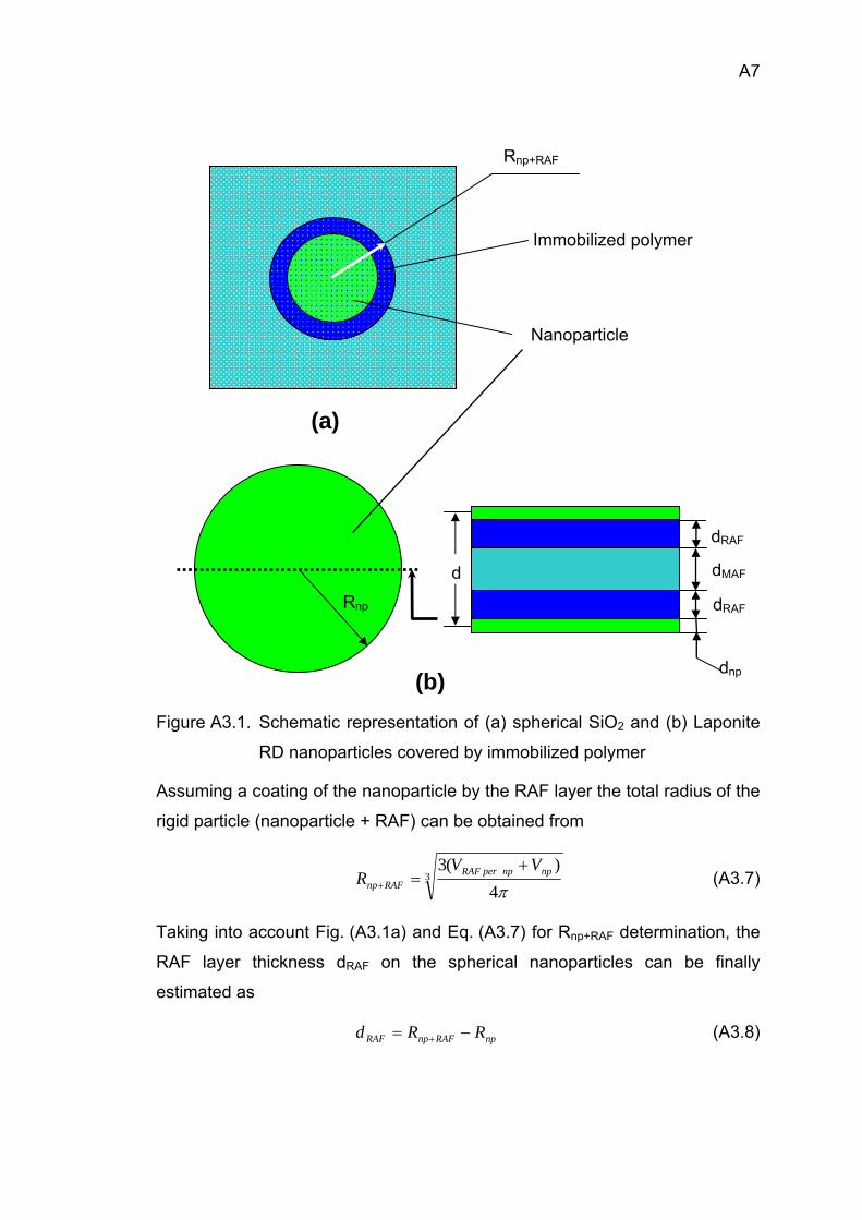
A7
Figure A3.1. Schematic representation of (a) spherical SiO2 and (b) Laponite
RD nanoparticles covered by immobilized polymer
Assuming a coating of the nanoparticle by the RAF layer the total radius of the
rigid particle (nanoparticle + RAF) can be obtained from
3
4)(3
πnpnpperRAF
RAFnp
VVR
+=+ (A3.7)
Taking into account Fig. (A3.1a) and Eq. (A3.7) for Rnp+RAF determination, the
RAF layer thickness dRAF on the spherical nanoparticles can be finally
estimated as
npRAFnpRAF RRd −= + (A3.8)
dMAF
Rnp+RAF
Immobilized polymer
Nanoparticle
(a)
dRAF
dnp
d
(b)
Rnp
dRAF

A8
For the Laponite RD filled systems the assumption that platelets are exfoliated
and covered from both sides by polymer is made (Fig. (A3.1b)). The volume of
the “sandwich” model VS of Laponite RD filled systems is equal to:
)2( MAFRAFnpSS dddAV ++= (A3.9)
where AS is the area of the platelet, dnp, dRAF and dMAF are the thicknesses of
the nanoparticle, immobilized and mobile polymer layer respectively. On the
other hand VS is also available from (Eq. (A3.10)) through volume fractions of
MAF (ϕMAF), RAF (ϕRAF) or nanoparticles (ϕnp).
np
Snp
RAF
SRAF
MAF
SMAFS
AdAdAdV
ϕϕϕ===
2 (A3.10)
To obtain the volume fractions the weight fractions, which are available from
the Δcp data (mMAF, mRAF and mnp), are divided by the densities (Eq. (A3.11)).
np
npnp
RAF
RAFRAF
MAF
MAFMAF
mmmρ
ϕρ
ϕρ
ϕ === ; (A3.11)
The density of PMMA at 25 °C is used as ρpolymer for MAF and RAF, and
nanofiller density ρnp is taken equal to that of SiO2. Consequently the RAF
layer thickness for Laponite RD based nanocomposites is estimated by
Eq. (A3.12).
2SRAF
RAFV
dϕ
= (A3.12)
where VS is determined from the last term in A3.10 with dnp = 1 nm. The
results for PMMA / SiO2 and PMMA / Laponite RD nanocomposites are given
in Fig. (5.3).

Liste der Veröffentlichung
Publikationen
1. Davtyan, S.P., Tonoyan, A.O., Sargsyan, A.G., Schick, C., Tataryan,
A.A. (2007). “Physical-mechanical, Thermophysical and
Superconducting Properties of Polymer-Ceramic Nanocomposites.” J.
of Materials Processing Technology, submitted
2. Tonoyan, A.O., Poghosyan M.G., Sargsyan, A.G., Schick, C., Davtyan,
S.P. (2006) “I. Crystallization kinetics under nonisothermal
polymerization conditions” Izvestija NAS RA and SEUA, V. 59, N 2, p.
193
3. Davtyan, S.P., Tonoyan, A.O., Sargsyan, A.G., Schick, C. (2007). “II.
Crystallization kinetics under nonisothermal polymerization conditions.”
Advanced Materials and technologies, Proceedings of the International
Conference, Tbilisi 10-11 May, 2006; Nova Science Publishers, Inc.,
Ney York, accepted
4. Sargsyan, A.G., Tonoyan, A.O., Davtyan, S.P., Schick, C. (2007). “The
amount of immobilized polymer in PMMA SiO2 nanocomposites
determined from calorimetric data.” European Polymer Journal, in press

Tagungsbeiträge
1. Manukyan, L.S., Tonoyan, A.O., Sargsyan, A.G., Davtyan, S.P.
“Research of Stationary Area Frontal Polymerization of the
Metallomonomers.” (talk) Enikolopyan readings, International Scientific
Conference of SEUA, October 7 – 9 (2003), Yerevan, Armenia; a member
of International Organization Committee, Youth scientific committee.
2. Hayrapetyan, S.M., Sargsyan, A.G., Tonoyan, A.O., Davtyan, S.P.
“Intercalation in Superconducting Polymer Nanocomposites.” (talk)
Enikolopyan readings, International Scientific Conference of SEUA, March
10 – 12 (2004), Yerevan, Armenia; a member of International
Organization Committee, Youth scientific committee.
3. Sargsyan, A.S., Thomas, Se., Wurm, A., Thomas, Sa., Schick, C.
European "Rigid Amorphous Fraction of Polymer Nanocomposites and
Semicrystalline Polymers." (poster) Conference Calorimetry and Thermal
Analysis for Environment, ECCTAE 2005, September 6 - 11 (2005);
Zakopane, Poland.
4. Sargsyan, A.S., Tonoyan, A.O., Davtyan, S.P., Schick, C. „Rigid
Amorphous Fraction in Polymer Nano-Composites“ (poster) DPG
Frühjarstagung - CMD21, March 26 – 31 (2006), Dresden, Germany.
5. Sargsyan, A.S., Tonoyan, A.O., Davtyan, S.P., Schick, C. “Relaxation of
rigid amorphous phase in polymers.” 9th Lähnwitzseminar on Calorimetry,
May 29 - June 1 (2006), Rostock, Germany.
6. Sargsyan, A.S., Wurm, A., Tonoyan, A.O., Davtyan, S.P., Schick, C.
“Influence of Plasticizer on Glass Transition of Systems Showing a Rigid
Amorphous Fraction.” (poster) Thermo international 2006, July 30 -
August 4 (2006), Boulder, Colorado.
7. Sargsyan, A.S., Tonoyan, A.O., Davtyan, S.P., Schick, C. “Rigid
Amorphous Fraction in Polymer Nano-Composite.” (poster) Thermo
international 2006, July 30 - August 4 (2006), Boulder, Colorado.
8. Sargsyan, A.S., Tonoyan, A.O., Davtyan, S.P., Schick, C. “Thermal
Characterization of PMMA SiO2 Nano-Composites Prepared by Different

Methods.” (talk) North American Thermal Analysis Society (NATAS) 34th
Annual Conference, August 6 - 9 (2006), Bowling Green, Kentucky, USA,
Perkin Elmer Student Award winner.
9. Sargsyan, A.S., Tonoyan, A.O., Davtyan, S.P., Schick, C. “Rigid
Amorphous Fraction in Polymer Nano-Composites.” (poster) North
American Thermal Analysis Society (NATAS) 34th Annual Conference,
August 6 - 9 (2006), Bowling Green, Kentucky, USA.
10. Sargsyan, A.S., Tonoyan, A.O., Davtyan, S.P., Schick, C. “When does the
rigid Amorphous Fraction in Polymer Nanocomposites Devitrify?” (poster)
North American Thermal Analysis Society (NATAS) 34th Annual
Conference, August 6 - 9 (2006), Bowling Green, Kentucky, USA.
11. Sargsyan, A.S., Tonoyan, A.O., Davtyan, S.P., Schick, C. “Calorimetric
Investigation of PMMA SiO2 Nano-Composites Prepared by Different
Methods.” (poster) The 9th European Symposium on Thermal Analysis
and Calorimetry, August 27 - 31 (2006), Krakow, Poland.
12. Sargsyan, A.G., Tonoyan, A.O., Davtyan, S.P., Schick, C. “Thermal
Characterization of PMMA SiO2 Nano-Composites Prepared by Different
Methods.” (talk) Enikolopyan readings, International Scientific Conference
of SEUA, October 4 – 6 (2006), Yerevan, Armenia; a member of
International Organization Committee, Youth scientific committee.
13. Sargsyan, A.G., Tonoyan, A.O., Davtyan, S.P., Schick, C. „Rigid
Amorphous Fraction in Polymer Nano-Composites“ (poster) Enikolopyan
readings, International Scientific Conference of SEUA, October 4 – 6
(2006), Yerevan, Armenia; a member of International Organization
Committee, Youth scientific committee.
14. Sargsyan, A.G., Tonoyan, A.O., Davtyan, S.P., Schick, C. „Quantification
of the Immobilized Fraction in Polymer Nano-Composites“ (poster) 71th
Annual Meeting of the Deutsche Physikalische Gesellschaft - spring
meeting of the Division Condensed Matter, March 26 – 30 (2007),
Regensburg, Germany.


CURRICULUM VITAE
1. Full name: Sargsyan Albert
family first
2. Date and place of birth: June 24th 1980; Yerevan, Armenia
3. Present address: Max-Planck Str. 3A, 18059 Rostock,
Germany
4. Affiliation, title and degree: University of Rostock, Institute of
Physics
PhD student, Master of Science in Chemistry
5. Short scientific biography:
2004 Research engineer “Chemical Technologies”, PhD course
at State Engineering University of Armenia
2002 M. Sci. in Organic Chemistry
Thesis: Liquid phase non-catalytic oxidation of
halogenvinylic compounds by molecular oxygen
State Engineering University of Armenia
2000 Diploma in Chemistry
State Engineering University of Armenia
6. Employment:
2004- University of Rostock, Inst. of Physics PhD Student, Polymer Physics 2000-2004 Centre of Expertise at the Ministry of Justice of Armenia Expert of the laboratory of Investigations by Physical- Chemical methods 2001-2002 Centre of Investigations of Molecule Structure, Institute of
Fine Organic Chemistry, Yerevan, Armenia Operator at the Laboratory of Mass spectroscopy
7. Field of specialization:
Polymer chemistry and technology, calorimetry, polymer
nanocomposites

Aknowledgements
I want to thank my DAAD “Sandwich Program” co-supervisors Prof. Dr.
Anahit Tonoyan, Yerevan, and Prof. Dr. Christoph Schick, Rostock, very much
for giving me the opportunity to carry out this work. The very essential and
fruitful discussions helped me to get a deeper insight into many current
problems of calorimetry and polymer nanocomposites. I would like to thank
Prof. Dr. Sevan Davtyan, Yerevan, for valuable discussions and ideas.
I am very grateful to all my colleges (former and present) for their
support and friendship.
PD Dr. Doris Pospiech and her colleagues from the Leibniz Institute of
Polymer Research, Dresden, I acknowledge for the important contribution to
the characterization and processing of polymer nanocomposite samples.
I am very thankful to International PhD Program – “IPP made in
Germany” (University of Rostock), for the possibility to present my work at
several international conferences. Financial support of through a stipend from
DAAD is gratefully acknowledged.
This work would not be possible without the serious support and help
from my family.


Erklärung
Ich versichere hiermit an Eides statt, dass ich die vorliegende Arbeit
selbstständig angefertigt und ohne fremde Hilfe verfasst habe, keine außer
den von mir angegebenen Hilfsmitteln und Quellen dazu verwendet habe und
die den benutzten Werken inhaltlich und wörtlich entnommenen Stellen als
solche kenntlich gemacht habe.
Rostock,
Albert Sargsyan
Recommended


