A Weighted Approach to Zero-Inflated PoissonRegression Models With Missing Data in Covariates.
Martin Lukusa. T.1?
, Shen-Ming Lee1 and Chin-Shang Li2
1. Department of Statistics, Feng Chia University, Taiwan.
2.Division of Biostatistics, Department of Public Health Sciences , UC, Davis, USA.
May 2014
Martin Lukusa. T.1?
, Shen-Ming Lee1 and Chin-Shang Li2 (1. Department of Statistics, Feng Chia University, Taiwan. [ 2pt] 2.Division of Biostatistics, Department of Public Health Sciences , UC, Davis, USA. [-2pt] )Modeling ZIP with incomplete Covariates May 2014 1 / 29

Table of Contents
1 Introduction
2 Estimating ZIP under no missings
3 Estimating ZIP under Missings CovariatesEstimating ZIP under Missings Covariates
4 Large Sample Properties
5 simulation Study
6 Empirical Study
Martin Lukusa. T.1?
, Shen-Ming Lee1 and Chin-Shang Li2 (1. Department of Statistics, Feng Chia University, Taiwan. [ 2pt] 2.Division of Biostatistics, Department of Public Health Sciences , UC, Davis, USA. [-2pt] )Modeling ZIP with incomplete Covariates May 2014 2 / 29

Introduction
Background Study
1 Count data cover considerable portion of data used in many fieldsincluding social sciences, medical, industrial, ecology and etc.
2 poisson regression model is the basic and natural model for countdata. See (Cameron and Trivedi, 1998)[1]).
3 Overdispersion problem: In practice, many count data have manyzeroes resulting to an overdispersed distribution or a skeweddistribution See (McCullagh and Nelder(1989)[10])
As Consequences
Assumption of mean=variance does not hold.
Poisson fit becomes questionable.
Need for advanced models able to account for overdispersion.
Martin Lukusa. T.1?
, Shen-Ming Lee1 and Chin-Shang Li2 (1. Department of Statistics, Feng Chia University, Taiwan. [ 2pt] 2.Division of Biostatistics, Department of Public Health Sciences , UC, Davis, USA. [-2pt] )Modeling ZIP with incomplete Covariates May 2014 3 / 29

Introduction
(Be Cont.)
Potential candidates for handling overdispersion are:
Negative binomial (NB)
Zero-Inflation Poisson (ZIP)
Negative Zero Inflated Binomial (NZIB)
Generalized Poisson Model (GP)
Hurdle models and other Truncated models
Interest: In the presence of overdispersion, we propose to fit countdata using Zero-Inflated Poisson (ZIP) Model.
Martin Lukusa. T.1?
, Shen-Ming Lee1 and Chin-Shang Li2 (1. Department of Statistics, Feng Chia University, Taiwan. [ 2pt] 2.Division of Biostatistics, Department of Public Health Sciences , UC, Davis, USA. [-2pt] )Modeling ZIP with incomplete Covariates May 2014 4 / 29
Introduction
Literature Review ZIP Model
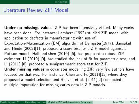
Under no missings values, ZIP has been intensively visited. Many workshave been done. For instance; Lambert (1992) studied ZIP model withapplication to decfects in manufacturing with use ofExpectation-Maximization (EM) algorithm of Dempster(1977). Jansakuland Hinde (2002)[11] proposed a score test for a ZIP model against aPoisson model. Hall and shen (2010) [6], has proposed a robust ZIPestimator, Li (2010) [9], has studied the lack of fit for parametric test, andLi (2011) [8], proposed a semiparametric score test for ZIP.Under missing values in covariates modelling ZIP, very few authors havefocused on that way. For instance, Chen and Fu(2011)[13] where theyproposed a model selection and Bhavna et al. (2011)[2] conducted amultiple imputation for missing caries data in ZIP models.
Martin Lukusa. T.1?
, Shen-Ming Lee1 and Chin-Shang Li2 (1. Department of Statistics, Feng Chia University, Taiwan. [ 2pt] 2.Division of Biostatistics, Department of Public Health Sciences , UC, Davis, USA. [-2pt] )Modeling ZIP with incomplete Covariates May 2014 5 / 29

Introduction
General Concepts of Zero-Inflation Poisson (ZIP) Model.
Let Yi = 0, 1, 2, · · · , n be count response variable, suct that Yi is amixture of two distributions. Yi degenerates at mass 0 with probability pior Yi is Poisson(µi ) random with probability 1− pi .Yi density probability function is given by:
P(Yi = y ; p, µ) = p + (1− p)e−µ, if y = 0; (1− p)e−µµy
y !, if y > 0.
Define p = H(u) as the mixing probability where H(u) =exp(u)
1 + exp(u)and
u = γTX . Similarly, µ = exp(u) is the poisson mean where u = βTX , and
where X =(1,XT ,ZT
)T, and here X and Z are univariate covariates.
Martin Lukusa. T.1?
, Shen-Ming Lee1 and Chin-Shang Li2 (1. Department of Statistics, Feng Chia University, Taiwan. [ 2pt] 2.Division of Biostatistics, Department of Public Health Sciences , UC, Davis, USA. [-2pt] )Modeling ZIP with incomplete Covariates May 2014 6 / 29

Introduction
ZIP can model simulteneously p, µ respectively by logistic and poisson
forms. We seek to estimate θ =(γT ,βT
)T, where γ =
(γ0,γ
T1 ,γ
T2
)Tand β =
(β0,β
T1 ,β
T2
)T. Let now define
P(Yi = 0|Xi ,Zi
)= H(γTXi ) + (1− H(γTXi )) exp(− exp(βTXi ))
= H(γTXi
)H−1
(γTXi + exp(βTXi )
), (1)
P(Yi > 0|Xi ,Zi
)= 1− P
(Yi = 0|Xi ,Zi
). (2)
Note that Zero-Inflated Poisson mean, denoted by E(Yi ) and its variancedenoted by Var(Yi ) of Yi are respectively expressed as follows
E(Yi ) =[1− H
(γTXi
)]exp
(βTXi
), and
Var(Yi ) =(1− H
(γTXi
))exp
(βTXi
){1 + H
(γTXi
)exp
(βTXi
)}.
Martin Lukusa. T.1?
, Shen-Ming Lee1 and Chin-Shang Li2 (1. Department of Statistics, Feng Chia University, Taiwan. [ 2pt] 2.Division of Biostatistics, Department of Public Health Sciences , UC, Davis, USA. [-2pt] )Modeling ZIP with incomplete Covariates May 2014 7 / 29

Estimating ZIP under no missings
Likelihood function (ZIP)
The likelihood function L(θ) is expressed by
L(θ) =n∏
i=1
[H(γTXi
)H−1
(γTXi + exp(βTXi )
)]I (yi=0)
n∏i=1
[(1− H(γTXi )
)exp(− exp(βTXi )
)[exp(βTXi )]yi
yi !
]I (yi>0)
. (3)
Applying the natural log to L(θ), we obtain the log-likelihood function `(θ) given by
`(θ) =n∑
i=1
[I (Yi = 0)
(log[H(γTXi
)]− log
[H(γTXi + exp(βTXi )
)])]
+n∑
i=1
[I (Yi > 0)
(log(1− H(γTXi )
)+(Yiβ
TXi − exp(βTXi )− logYi !))]
.
(4)
which can be optimized by maximum likelihood estimation method (MLE/EM al.) to find θas in Lambert (1992).
Martin Lukusa. T.1?
, Shen-Ming Lee1 and Chin-Shang Li2 (1. Department of Statistics, Feng Chia University, Taiwan. [ 2pt] 2.Division of Biostatistics, Department of Public Health Sciences , UC, Davis, USA. [-2pt] )Modeling ZIP with incomplete Covariates May 2014 8 / 29

Estimating ZIP under no missings
Model Estimation Complete Data(Ideal)
Under no missings, the estimating equation (E.E) based on score functions is given by
Un
(θ)
=1√n
∂`(θ)
∂θT=
1√n
∂`(θ)
∂γ∂`(θ)
∂β
=1√n
n∑i=1
Si(θ), (5)
with Si(θ)
=(STi1
(θ),ST
i2
(θ))T
, where Si1(θ)
and Si2(θ)
are respectively given by
Si1(θ)
= XiH(γTXi + exp(βTXi )
){I (Yi = 0)− HγTXi
H(γTXi + exp(βTXi )
)}, (6)
Si2(θ)
= Xi
{[Yi −
(1− H(γTXi )
)exp(βTXi )
]}+ exp(βTXi )Si1
(θ). (7)
Since, E[Un
(θ)]
= 0, this implies that Un
(θ)
is unbiased (E.E). Solving for Un
(θ)
= 0, we
obtain the maximum likelihood estimator (MLE) θF of θ.Some Optimization Techniques; for instance, NR (Jansakul and Hinde (2002)[11]), EMalgorithm (Lambert(1992)[5]),ITRLS (Li (2010)[9]), MCMC under Bayesian set up.
Martin Lukusa. T.1?
, Shen-Ming Lee1 and Chin-Shang Li2 (1. Department of Statistics, Feng Chia University, Taiwan. [ 2pt] 2.Division of Biostatistics, Department of Public Health Sciences , UC, Davis, USA. [-2pt] )Modeling ZIP with incomplete Covariates May 2014 9 / 29

Estimating ZIP under Missings Covariates
Missing Data Concepts
Consider the data {Yi , Xi , Zi , Wi , δi }, i = 1, · · · , n.Denote
V =(Z ,W
)T. The missing mechanisms play important role in dealing
with missing problems. Rubin(1976) distinguishes three processes ofmissing as follows:
1 Missing Completely at Random(MCAR) with selection probabilitygiven by
P(δi = 1|Yi ,Xi ,Vi ) = πi ,2 Missing at Random(MAR) where the selection probability is expressed
by
P(δi = 1|Yi ,Xi ,Vi ) = π(Yi ,Vi ),3 Missing at Not Random (MNAR) where the selection probability is
given by
P(δi = 1|Yi ,Xi ,Vi ) = π(Yi ,Xi ,Vi ),
MCAR and MAR refer to ignorable missings while MNAR refers tononignorable missings.
Martin Lukusa. T.1?
, Shen-Ming Lee1 and Chin-Shang Li2 (1. Department of Statistics, Feng Chia University, Taiwan. [ 2pt] 2.Division of Biostatistics, Department of Public Health Sciences , UC, Davis, USA. [-2pt] )Modeling ZIP with incomplete Covariates May 2014 10 / 29

Estimating ZIP under Missings Covariates Estimating ZIP under Missings Covariates
Complete Cases Analysis (CC Method)
Define δi = 1, when Xi is observed and δi = 0, otherwise.Under MAR,define the selection probability P(δi = 1|Yi ,Xi ,Vi ) = π(Yi ,Vi ).ZIP CC estimating function denoted by UCC ,n
(θ)
is expressed as follows
UCC ,n
(θ)
=1√n
n∑i=1
δiSi(θ)
=1√n
n∑i=1
δi
(Si1(θ)
Si2(θ)) , (8)
where Si1(θ)
and Si2(θ)
are respectively given in expressions (6) and (7).
The solution θCC is obtained when solving UCC ,n
(θ)
= 0.
1 It can be established that under MAR, E[UCC ,n
(θ)]6= 0.
2 Therefore, UCC ,n
(θ)
is biased.
3 CC inference mostly inefficiency due to cases deletion.
Martin Lukusa. T.1?
, Shen-Ming Lee1 and Chin-Shang Li2 (1. Department of Statistics, Feng Chia University, Taiwan. [ 2pt] 2.Division of Biostatistics, Department of Public Health Sciences , UC, Davis, USA. [-2pt] )Modeling ZIP with incomplete Covariates May 2014 11 / 29

Estimating ZIP under Missings Covariates Estimating ZIP under Missings Covariates
Inverse Probability Weighting (IPW) Method
BackgroundInspired from Horvitz-Thomsom (H-T) estimator (1952)[7], separately,Flanders and Greenland (1991)[12] and Zhao and Lipsitz (1992)[14]extended the H-T estimator and proposed the IPW estimator. Recently,Creemers et al.(2012)[3] proposed general concepts for nonparametricweighting estimating function under MAR. The IPW inversely weights theobserved data with some weights π
(Yi ,Vi
)in order to reduce the bias due
to incomplete cases deletion. This article implements the IPW toZero-Inflated Poisson when π
(Yi ,Vi
)is nonparametric.
Martin Lukusa. T.1?
, Shen-Ming Lee1 and Chin-Shang Li2 (1. Department of Statistics, Feng Chia University, Taiwan. [ 2pt] 2.Division of Biostatistics, Department of Public Health Sciences , UC, Davis, USA. [-2pt] )Modeling ZIP with incomplete Covariates May 2014 12 / 29

Estimating ZIP under Missings Covariates Estimating ZIP under Missings Covariates
Let δi = 1 if Xi is observed, and δi = 0 elsewhere. Under MAR, the selection probability ofobserving Xi is
P(δi = 1|Yi ,Xi ,Vi ) = π(Yi ,Vi ),
where Vi =(Zi ,Wi
)T. In this article, Zi is always observed and Wi is a surrogate of Xi . Wi is
available and independent of Yi given(Xi ,Zi
). The inverse probability weighting (E.E) ZIP
respectively with parametric and nonparametric π(.) are given by:
UWp,n
(θ,φ
)=
1√n
n∑i=1
δi
π(Yi ,Vi ;φ
)Si(θ) =1√n
n∑i=1
δi
π(Yi ,Vi ;φ
) (Si1(θ)Si2(θ)
)(9)
Uws,n
(θ, π
)=
1√n
n∑i=1
δi
π(Yi ,Vi
)Si(θ) =1√n
n∑i=1
δi
π(Yi ,Vi
) (Si1(θ)Si2(θ)
). (10)
where Si1(θ) and Si2(θ) are respectively given in expressions (6) and (7). We obtainconsistent estimator of θ denoted by θWs using UWs,n
(θ, π
)= 0; similarly, θWp using
UWp,n
(θ,φ
)= 0.
Martin Lukusa. T.1?
, Shen-Ming Lee1 and Chin-Shang Li2 (1. Department of Statistics, Feng Chia University, Taiwan. [ 2pt] 2.Division of Biostatistics, Department of Public Health Sciences , UC, Davis, USA. [-2pt] )Modeling ZIP with incomplete Covariates May 2014 13 / 29
Estimating ZIP under Missings Covariates Estimating ZIP under Missings Covariates
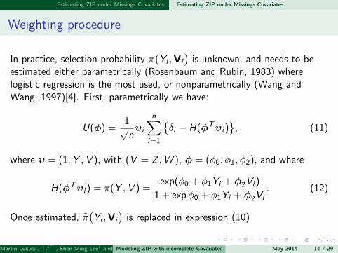
Weighting procedure
In practice, selection probability π(Yi ,Vi
)is unknown, and needs to be
estimated either parametrically (Rosenbaum and Rubin, 1983) wherelogistic regression is the most used, or nonparametrically (Wang andWang, 1997)[4]. First, parametrically we have:
U(φ) =1√nυi
n∑i=1
{δi − H(φTυi )
}, (11)
where υ = (1,Y ,V ), with (V = Z ,W ), φ = (φ0, φ1, φ2), and where
H(φTυi ) = π(Y ,V ) =exp(φ0 + φ1Yi + φ2Vi )
1 + expφ0 + φ1Yi + φ2Vi. (12)
Once estimated, π(Yi ,Vi
)is replaced in expression (10)
Martin Lukusa. T.1?
, Shen-Ming Lee1 and Chin-Shang Li2 (1. Department of Statistics, Feng Chia University, Taiwan. [ 2pt] 2.Division of Biostatistics, Department of Public Health Sciences , UC, Davis, USA. [-2pt] )Modeling ZIP with incomplete Covariates May 2014 14 / 29

Estimating ZIP under Missings Covariates Estimating ZIP under Missings Covariates
Weighting procedure (Be cont.)
Second, the selection probability is nonparametrically estimated. We alsoassume that covariates are categorical. Let v1, v2, · · · , vm denote thedistinct values of Vi , for v ∈
[v1, v2, · · · , vm
]; the nonparametric estimator
of π(Yi ,Vi
)is given by the following expression:
π(y , v) =
∑ni=1 δi I
(Yi = y ,Vi = v
)∑ni=1 I
(Yi = y ,Vi = v
) , (13)
where V =(Z ,W
)T, and I
(.)
is indicator function. Once estimated,π(Yi ,Vi
)is replaced in expression (10). Next on , we focused only case
where selection probability is nonparametric.
Martin Lukusa. T.1?
, Shen-Ming Lee1 and Chin-Shang Li2 (1. Department of Statistics, Feng Chia University, Taiwan. [ 2pt] 2.Division of Biostatistics, Department of Public Health Sciences , UC, Davis, USA. [-2pt] )Modeling ZIP with incomplete Covariates May 2014 15 / 29
Large Sample Properties
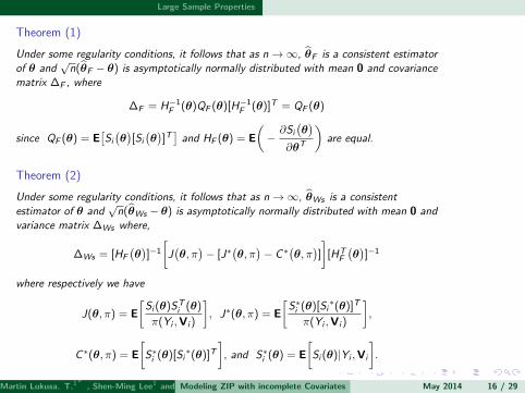
Theorem (1)
Under some regularity conditions, it follows that as n→∞, θF is a consistent estimatorof θ and
√n(θF − θ) is asymptotically normally distributed with mean 0 and covariance
matrix ∆F , where
∆F = H−1F (θ)QF (θ)[H−1
F (θ)]T = QF (θ)
since QF (θ) = E[Si(θ)[Si(θ)]T]and HF (θ) = E
(−∂Si(θ)
∂θT
)are equal.
Theorem (2)
Under some regularity conditions, it follows that as n→∞, θWs is a consistentestimator of θ and
√n(θWs − θ) is asymptotically normally distributed with mean 0 and
variance matrix ∆Ws where,
∆Ws = [HF
(θ)]−1
[J(θ, π
)− [J∗
(θ, π
)− C ∗(θ, π)]][HT
F
(θ)]−1
where respectively we have
J(θ, π) = E
[Si (θ)ST
i (θ)
π(Yi ,Vi )
], J∗(θ, π) = E
[S∗i (θ)[Si
∗(θ)]T
π(Yi ,Vi )
],
C ∗(θ, π) = E
[S∗i (θ)[Si
∗(θ)]T], and S∗
i (θ) = E
[Si (θ)|Yi ,Vi
].
Martin Lukusa. T.1?
, Shen-Ming Lee1 and Chin-Shang Li2 (1. Department of Statistics, Feng Chia University, Taiwan. [ 2pt] 2.Division of Biostatistics, Department of Public Health Sciences , UC, Davis, USA. [-2pt] )Modeling ZIP with incomplete Covariates May 2014 16 / 29

simulation Study
Settings A simulation study is conducted to investigate the finite sampleproperties performance under different estimator. We consider thefollowing
θF which is the complete data estimator of θ.
θCC which is the complete cases estimator of θ.
θWt which is the true weight IPW estimator of θ.
θWs which is the semiparametric IPW estimator of θ.
We chose the sample size n to be equal to 500 and 1000 observations, andtotal number of simulations was set to 1000 replications. We consideredcovariates to be univariate and categorical. For each senario, we computethe bias, the asymptotic standard error (ASE), the standarddeviation(SD), and the 95% confidence interval coverage probability (CP).We considered covariates X and Z such that X were generated fromuniform distribution U(−1, 2) and Z is binomial B(n, p) where p is theprobability of success equals to 0.5. We generated a binary surrogatevariable W such that W = 1 if X ≥ 0 and W = 0 otherwise.
Martin Lukusa. T.1?
, Shen-Ming Lee1 and Chin-Shang Li2 (1. Department of Statistics, Feng Chia University, Taiwan. [ 2pt] 2.Division of Biostatistics, Department of Public Health Sciences , UC, Davis, USA. [-2pt] )Modeling ZIP with incomplete Covariates May 2014 17 / 29

simulation Study
cont. The count response (ZIP) was generated as followsY = p ∗ 0 + (1− p) ∗ pois(λ) here p is the mixing proportion and λ thepoisson mean. They were respectively expressed asp = H(γ1 + γ2 ∗ X + γ3 ∗ Z ) and λ = exp(−β1 − β2 ∗ X − β3 ∗ Z ), with
θ =(γT ,βT
)T, where γ =
(θ1,θ2,θ3
)T,β =
(θ1,θ2,θ3
)Tsuch that
θ = (−1,−1, 0.5, 1, 0.7, 1). To account for the missing covariates in X ,where δi = 1 if X is observed and δi = 0 otherwise, we used the selectionprobability defined by logistic regression such asH(−η1 − η2Y ∗ I (Y < k∗)− η3(1− I (Y < k∗) + η4Z + η5W ), where thecut points was k∗ = 6. We considered two situations as follows:
1 When δ was generated using the selection probability withη = c(−1, 0.3, 10,−0.5, 1), the missng rate (mrate) was 33%.
2 When δ was generated using the selection probability withη = c(−1, .5, 1, .7, 1), the missng rate (mrate) was 68%.
Results of simulations are found into table1, table2 and table3.
Martin Lukusa. T.1?
, Shen-Ming Lee1 and Chin-Shang Li2 (1. Department of Statistics, Feng Chia University, Taiwan. [ 2pt] 2.Division of Biostatistics, Department of Public Health Sciences , UC, Davis, USA. [-2pt] )Modeling ZIP with incomplete Covariates May 2014 18 / 29

simulation Study
Table1: Simulation
Table: Result1 :: 500 obs , 1000 draws and mrate 0.33 .
par estimate θF θCC θWt θWs
γ2 Bias -0.0258 -0.5708 -0.0627 -0.0558SD 0.1575 0.2895 0.2927 0.2338
ASE 0.1527 0.2768 0.2770 0.2088CP 0.9470 0.4630 0.9430 0.9040
β2 Bias -0.0008 -0.0393 -0.0012 -0.0075SD 0.0260 0.0279 0.0317 0.0284
ASE 0.0261 0.0280 0.0299 0.0262CP 0.9570 0.7020 0.9310 0.9260
Martin Lukusa. T.1?
, Shen-Ming Lee1 and Chin-Shang Li2 (1. Department of Statistics, Feng Chia University, Taiwan. [ 2pt] 2.Division of Biostatistics, Department of Public Health Sciences , UC, Davis, USA. [-2pt] )Modeling ZIP with incomplete Covariates May 2014 19 / 29

simulation Study
Table2: Simulation
Table: Result2 :: 500 obs , 1000 draws and mrate 0.67 .
par estimate θF θCC θWt θWs
γ2 Bias -0.0258 -0.5606 -0.0626 -0.0558SD 0.1575 0.2897 0.2927 0.2339
ASE 0.1527 0.2769 0.2772 0.2088CP 0.9470 0.4780 0.9440 0.9060
β2 Bias -0.0008 -0.0388 -0.0012 -0.0075SD 0.0260 0.0281 0.0317 0.0285
ASE 0.0261 0.0282 0.0300 0.0263CP 0.9570 0.7180 0.9340 0.9280
Martin Lukusa. T.1?
, Shen-Ming Lee1 and Chin-Shang Li2 (1. Department of Statistics, Feng Chia University, Taiwan. [ 2pt] 2.Division of Biostatistics, Department of Public Health Sciences , UC, Davis, USA. [-2pt] )Modeling ZIP with incomplete Covariates May 2014 20 / 29

simulation Study
Table3: Simulation
Table: Result3: 1000 obs , 1000 draws and mrate 0.33 .
par estimate θF θCC θWt θWs
γ2 Bias -0.0065 -0.5368 -0.0222 -0.0177SD 0.1086 0.1964 0.1976 0.1628
ASE 0.1068 0.1905 0.1921 0.1500CP 0.9440 0.1620 0.9470 0.9330
β2 Bias 0.0000 -0.0389 0.0003 -0.0035SD 0.0187 0.0190 0.0214 0.0195
ASE 0.0184 0.0197 0.0213 0.0188CP 0.9450 0.5050 0.9550 0.9380
Martin Lukusa. T.1?
, Shen-Ming Lee1 and Chin-Shang Li2 (1. Department of Statistics, Feng Chia University, Taiwan. [ 2pt] 2.Division of Biostatistics, Department of Public Health Sciences , UC, Davis, USA. [-2pt] )Modeling ZIP with incomplete Covariates May 2014 21 / 29

Empirical Study
Motorcycle Violations Speed Regulations (Taiwan Survey)
Period and Space
1 The survey was conducted during the year 2007 accross Taiwan.2 source: Ministry of transport (ROC).3 The total number of respondents (observations) was 7386.4 Most of respondents were from Taipei, Taoyun, Gaoshong, and Hualien. Only few
respondents from the other remaining cities and counties have been recorded.
Variables
1 Y.Violation , count variable :: gives the number of time the respondent has been foundguilty of violating speed regulations.
2 X2.Age Age, categorical variable where:: (1) < 18 years old, (2) 18− 19 years old, (3)20− 29 years old, (4) 30− 39 years old, (5) 40− 49 years old, and (6) >= 50 years old.
3 X3 Education Levels, categorical variable where (1) under high school, (2) high school,(3) colleage and above.
4 X7 Kilometer (Km), continuous variable where (1) < 1000 Km, (2) 1,000-2,999 Km, (3)3000-9999 Km, and over (4) 10,000 Km in a year.
5 X8 Engine power, categorical variable where (1) under 50cc. (2) 50 - 249cc. (3)250-549cc (4) over 550cc.
Martin Lukusa. T.1?
, Shen-Ming Lee1 and Chin-Shang Li2 (1. Department of Statistics, Feng Chia University, Taiwan. [ 2pt] 2.Division of Biostatistics, Department of Public Health Sciences , UC, Davis, USA. [-2pt] )Modeling ZIP with incomplete Covariates May 2014 22 / 29

Empirical Study
Table: Variable Descriptions .
Variable Definition Possible Val N OBS Missing I % II %
N.Violations(Y) number of violations in a year 1-7 7386 7386 0 91% are 0 9% > 0Distance(X) Km covered per year 1-4 7386 6262 1124 15% missing 85% obsX.Dummy 2 1, 000 ≤ X < 2, 999 Km 0-1 7386 6262 1124 25% of X=2X.Dummy3 3, 000 ≤ X < 9, 999 Km 0-1 7386 6262 1124 12.8% of X=3X.Dummy3 ≥ 10000 Km 0-1 7386 6262 1124 12.8% of X=4Engine (Z) ≤ 250cc 0-1 7386 7386 0 88% has ≤250cc 12%Age (W) ≤ 40years old 0-1 7386 7386 0 72.5% has ≤40 17.5%
1 X.Dummy1 X < 1,000 Km is considered as baseline.2 W :: Age (X2) is chosen as the most potential the surrogate.3 The correlation (X, W) is 0.10, not so enough.
Martin Lukusa. T.1?
, Shen-Ming Lee1 and Chin-Shang Li2 (1. Department of Statistics, Feng Chia University, Taiwan. [ 2pt] 2.Division of Biostatistics, Department of Public Health Sciences , UC, Davis, USA. [-2pt] )Modeling ZIP with incomplete Covariates May 2014 23 / 29

Empirical Study
Output 1. Histogram for Count response variable
Figure: Awesome figure
Martin Lukusa. T.1?
, Shen-Ming Lee1 and Chin-Shang Li2 (1. Department of Statistics, Feng Chia University, Taiwan. [ 2pt] 2.Division of Biostatistics, Department of Public Health Sciences , UC, Davis, USA. [-2pt] )Modeling ZIP with incomplete Covariates May 2014 24 / 29

Empirical Study
Diagnostic MAR
δ = 1 if X 6= NA and 0 otherwise (Probability of missingness). TestingMAR, we fit logistic regression π(δ = 1|observed data).
π(Y ,Z ,W ) = Pr(δ = 1|Y ,Z ,W ) = H(αTU),
where U = (1,Y T ,ZT ,W T ). The selection probability is given by
π(Y ,Z ,W ) = H(0.854631 + 0.051814Y + 0.047927Z − 0.071278W )
with coefficients from the below table.
Coef. Estimate Std.Err Pr(> |z |)α0 0.854631 0.005223 < 2e-16α1 0.051814 0.008466 9.81e-10α2 0.047927 0.013212 0.000288α3 -0.071278 0.009311 2.18e-14
From the above results, the probability of missing is strongly depending onobserved data. That support MAR assumption. Note here that α isnuissance parameter.
Martin Lukusa. T.1?
, Shen-Ming Lee1 and Chin-Shang Li2 (1. Department of Statistics, Feng Chia University, Taiwan. [ 2pt] 2.Division of Biostatistics, Department of Public Health Sciences , UC, Davis, USA. [-2pt] )Modeling ZIP with incomplete Covariates May 2014 25 / 29

Empirical Study
Output 2. Regression ZIP
Table: Outputs Regression ZIP model
Par. Complete Cases Semiparametric IPW
Coef. θCC Std.Err Pr(> |z |) θWs Std.Err Pr(> |z |)
γ0 2.6854 0.1723 0.0000 2.8181 0.1790 0.0000γ1 -0.5747 0.2014 0.0043 -0.5766 0.2059 0.0051γ2 -0.8672 0.2001 0.0000 -0.8564 0.2077 0.0000γ3 -1.0602 0.2165 0.0000 -1.0359 0.2277 0.0000γ4 -2.1884 0.1694 0.0000 -2.1705 0.1647 0.0000
β0 -0.2976 0.1466 0.0423 -0.3190 0.1659 0.0546
β1 0.0960 0.1608 0.5505 0.0988 0.1790 0.5812
β2 0.1530 0.1592 0.3365 0.1576 0.1811 0.3840
β3 0.3802 0.1705 0.0258 0.4100 0.1961 0.0366
β4 0.2033 0.1093 0.0627 0.2235 0.1118 0.0456
Martin Lukusa. T.1?
, Shen-Ming Lee1 and Chin-Shang Li2 (1. Department of Statistics, Feng Chia University, Taiwan. [ 2pt] 2.Division of Biostatistics, Department of Public Health Sciences , UC, Davis, USA. [-2pt] )Modeling ZIP with incomplete Covariates May 2014 26 / 29

Empirical Study
Where Θ = (γ, β), and where γ = (γ0, γ1, γ2), and β = (β0, β1, β2) arerespectively the logistic and poisson components. The mixing proportionand the poisson mean for complete cases and inverse probability weightingare respectively expressed byPCC = H(2.6854− 0.5747D1− 0.8672D2− 1.0602D3− 2.1884Z ) andµCC = exp(−0.2976 + 0.0960D1 + 0.1530D2 + 0.3802D3− 2.1884Z ),PWs = H(2.8181− 0.5766D1 + 0.0988D2 + 1.0359D3− 2.1705Z ) andµWs = exp(−0.3190 + 0.0988D1 + 0.1576D2 + 0.4100D3 + 0.2235Z ).The predicted function for random Y can be put in the following way.
Y ∼
{deg(0), with probability P,
Poisson(µ), with probability 1− P.
where P = PCC or PWs and µ = µCC or µWs .
Martin Lukusa. T.1?
, Shen-Ming Lee1 and Chin-Shang Li2 (1. Department of Statistics, Feng Chia University, Taiwan. [ 2pt] 2.Division of Biostatistics, Department of Public Health Sciences , UC, Davis, USA. [-2pt] )Modeling ZIP with incomplete Covariates May 2014 27 / 29

Empirical Study
Discussion
1 The histogram has a skew on the left especially at point 0, showing aZero Inflated poisson distribution with( 91%) of zeroes.
2 The empirical study shows that our proposed method thesemiparametric inverse probability weighting for zero inflated poissonprovides acceptable results.
3 In addition, IPW performance is challenged by CC method. That isdue to the fact that the surrogate variable (W) has little contributionto (X).The correlation (X, W) is 0.10, and very big proportion ofzeros tends to support more for logit component than poisson.
4 The CC method performance is due to the percent of missing (15 %only) and big sample size.
As future work, other methods recommended in literature such as multipleimputations parametric/nonparametric and empirical multiple imputationcan be used to see how ZIP-IPW performs comparely to those others.Find other surrogate variables having strong relation with variable havingmissing.
Martin Lukusa. T.1?
, Shen-Ming Lee1 and Chin-Shang Li2 (1. Department of Statistics, Feng Chia University, Taiwan. [ 2pt] 2.Division of Biostatistics, Department of Public Health Sciences , UC, Davis, USA. [-2pt] )Modeling ZIP with incomplete Covariates May 2014 28 / 29

Empirical Study
Thank you for your Attention
Martin Lukusa. T.1?
, Shen-Ming Lee1 and Chin-Shang Li2 (1. Department of Statistics, Feng Chia University, Taiwan. [ 2pt] 2.Division of Biostatistics, Department of Public Health Sciences , UC, Davis, USA. [-2pt] )Modeling ZIP with incomplete Covariates May 2014 29 / 29

Empirical Study
Cameron, A.C and Trividi, P.K.Regression Analysis of Count Data”.Cambridge University Press, thirteenth edition, 1998.
Bhavna,T.P, Preisser,J.S, Stearn,S.C, and Rosier,R.G.Multiple imputation of dental caries data using a zero inflated poissonregression models.J public Health Dent., 1:71–78, 2011.
Creemers,A, Aerts, M, Hens, N, and Molenberghs, G.A nonparametric approach to weighted estimating equations forregression analysis with missing covariates.Computational Statistics and Data Analysis, 56:100–113, 2012.
Wang, C.Y, Wang,S, Zhao,L.P, and Ou, S.T.Weighted semiparametric estimation in regression with missingcovariates data.Journal of American Statistical Association, 92:512–525, 1997.
Lambert, D.
Martin Lukusa. T.1?
, Shen-Ming Lee1 and Chin-Shang Li2 (1. Department of Statistics, Feng Chia University, Taiwan. [ 2pt] 2.Division of Biostatistics, Department of Public Health Sciences , UC, Davis, USA. [-2pt] )Modeling ZIP with incomplete Covariates May 2014 29 / 29

Empirical Study
Zero-inflated poisson regression, with an application to defects inmanufacturing.Technometrics, 34:1–14, 1992.
Hall, D.B and Shen,J.Robust estimation for zero-inflated poisson regression.Scandinavian Journal of Statistics, 37:237–252, 2010.
D.G Horvitz and D.J Thomson.A generalization of sampling without replacement.Journal of The American Statistics Association, 47:663–685, 1952.
Chin-Shang , Li.Score test for semiparametric zero-inflated poisson models.International Journal of Statistics and Probability, 1:1–7, 2012.
Chin-Shang ,Li.A lack-of-fit test for parametric zero-inflated poisson zero-inflatedpoisson models.Computational and Simulation, 81:1081–1098, 2010.
Martin Lukusa. T.1?
, Shen-Ming Lee1 and Chin-Shang Li2 (1. Department of Statistics, Feng Chia University, Taiwan. [ 2pt] 2.Division of Biostatistics, Department of Public Health Sciences , UC, Davis, USA. [-2pt] )Modeling ZIP with incomplete Covariates May 2014 29 / 29

Empirical Study
McCullagh,P and Nelder,J.Generalized linear models.1989.
Jansakul, N and Hinde,J.P.Score test for zero-inflated poisson models.Computational Statistics and Data Analysis, 40:75–96, 2002.
Flanders, W.D. and Greenland, S.Analytic methods for two-stage casecontrol studies and other stratifieddesigns.Statistics in Medecine, 10:739–747, 1991.
Chen, X.D and Fu,Y.Z.Model selection for zero-inflatated regression with missing covariates.Computational Statistics and Data Analysis, 55:765–773, 2011.
Zhao,L.P and Lipsitz,S.Design and analysis of two-stage studies.Journal of stat. in Medecine, 11:769–782, 1992.
Martin Lukusa. T.1?
, Shen-Ming Lee1 and Chin-Shang Li2 (1. Department of Statistics, Feng Chia University, Taiwan. [ 2pt] 2.Division of Biostatistics, Department of Public Health Sciences , UC, Davis, USA. [-2pt] )Modeling ZIP with incomplete Covariates May 2014 29 / 29
Recommended