8/8/2019 PSTS 23344
http://slidepdf.com/reader/full/psts-23344 1/67
Chapter 1
Introduction to Communication Systems
Analog and Digital Communication SystemsA communication system conveys information from its source to a destination
some distance away. There are so many different applications of communication systems
that we cannot attempt to cover every type. Nor can we discuss in detail all the individual
parts that make up a specific system. A typical system involves numerous componentsthat run the gamut of electrical engineering-circuits, electronics, electromagnetic signal
processing, microprocessors, and communication networks, to name a few of the relevant
fields. Moreover, a piece-by-piece treatment would obscure the essential point that acommunication system is an integrated whole that really does exceed the sum of its parts.
We therefore approach the subject from a more general viewpoint. Recognizing
that all communication systems have the same basic function of information transfer,
we'll seek out and isolate the principles and problems of conveying information inelectrical form. These will be examined in sufficient depth to develop analysis and design
methods suited to a wide range of applications.
Information, Messages, and SignalsClearly, the concept of information is central to communication. But information
is a loaded word, implying semantic and philosophical notions that defy precise
definition. We avoid these difficulties by dealing instead with the message, defined as the
physical manifestation of information as produced by the source. Whatever form themessage takes, the goal of a communication system is to reproduce at the destination an
acceptable replica of the source message.
There are many kinds of information sources, including machines as well as people, and messages appear in various forms. Nonetheless, we can identify two distinct
message categories, analog and digital. This distinction, in turn, determines the criterion
for successful communication.
8/8/2019 PSTS 23344
http://slidepdf.com/reader/full/psts-23344 2/67
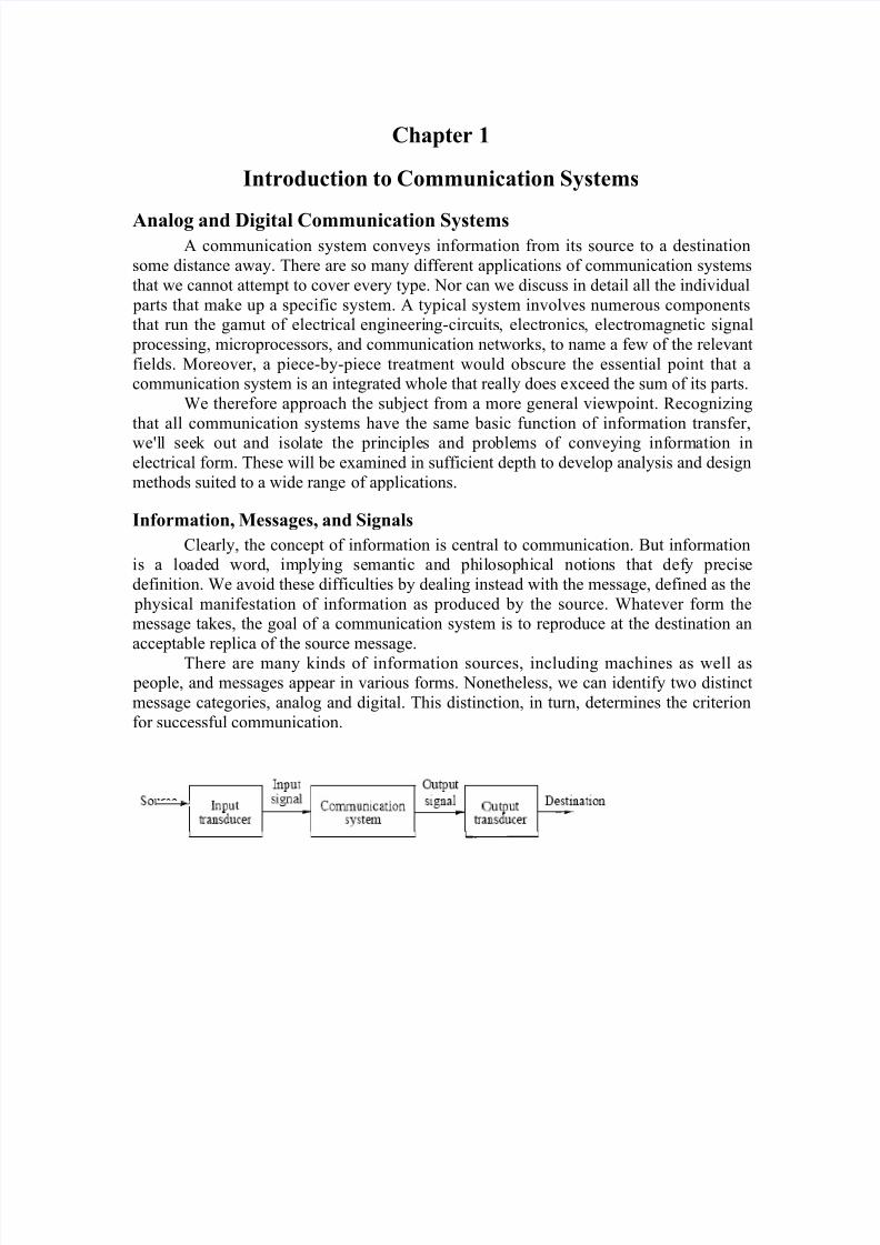
Fig 1.1 Communication system with input and output transducers
An analog message is a physical quantity that varies with time, usually in asmooth and continuous fashion. Examples of analog messages are the acoustic pressure
produced when you speak, the angular position of an aircraft gyro, or the light intensity at
some point in a television image. Since the information resides in a time-varyingwaveform, an analog communication system should deliver this waveform with a
specified degree of fidelity.A digital message is an ordered sequence of symbols selected from a finite set of
discrete elements. Examples of digital messages are the letters printed on this page, a
listing of hourly temperature readings, or the keys you press on a computer keyboard.
Since the information resides in discrete symbols, a digital communication system should
deliver these symbols with a specified degree of accuracy in a specified amount of time.Whether analog or digital, few message sources are inherently electrical.
Consequently, most communication systems have input and output transducers as
shown in Fig. 1.1. The input transducer converts the message to an electrical signal, say a
voltage or current, and another transducer at the destination converts the output signal tothe desired message form. For instance, the transducers in a voice communication system
could be a microphone at the input and a loudspeaker at the output. We'll assumehereafter that suitable transducers exist, and we'll concentrate primarily on the task of
signal transmission. In this context the terms signal and message will be used
interchangeably since the signal, like the message, is a physical embodiment of
information.
Elements of a Communication System
8/8/2019 PSTS 23344
http://slidepdf.com/reader/full/psts-23344 3/67
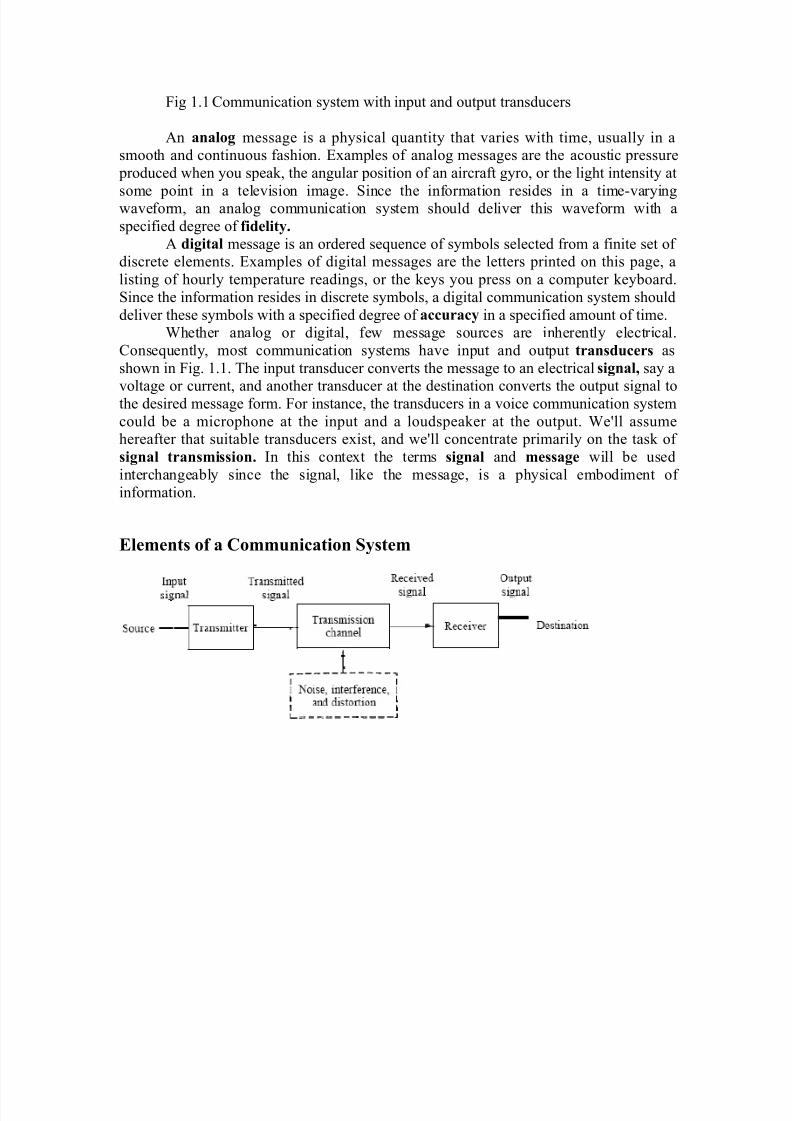
Fig 1.2 Elements of a communication system
Figure 1.2 depicts the elements of a communication system, omitting transducers
but including unwanted contaminations. There are three essential parts of anycommunication system, the transmitter, transmission channel, and receiver. Each pat
plays a particular role in signal transmission, as follows.
The transmitter processes the input signal to produce a transmitted signal suitedto the characteristics of the transmission channel. Signal processing for transmission
almost always involves modulation and may also include coding.The transmission channel is the electrical medium that bridges the distance from
source to destination. It may be a pair of wires, a coaxial cable, Sr a radio wave or laser beam. Every channel introduces some amount of transmission loss or attenuation, so the
signal power progressively decreases with increasing distance.
The receiver operates on the output signal from the channel in preparation for
delivery to the transducer at the destination. Receiver operations include amplification tocompensate for transmission loss, and demodulation and decoding to reverse the signal-
processing performed at the transmitter. Filtering is another important function at thereceiver, for reasons discussed next.
Various unwanted undesirable effects crop up in the course of signal transmission.
Attenuation is undesirable since it reduces signal strength at the receiver. More serious,
however, are distortion, interference, and noise, which appear as alterations of the signalshape. Although such contaminations may occur at any point, the standard convention is
to blame them entirely on the channel, treating the transmitter and receiver as being ideal.
Figure 1.2 reflects this convention.Distortion is waveform perturbation caused by imperfect response of the system
to the desired signal itself. Unlike noise and interference, distortion disappears when the
signal is turned off. If the channel has a linear but distorting response, then distortion may be corrected, or at least reduced, with the help of special filters called equalizers.
Interference is contamination by extraneous signals from human sources-other
transmitters, power lines and machinery, switching circuits, and so on. Interferenceoccurs most often in radio systems whose receiving antennas usually intercept several
signals at the same time. Radio-frequency interference (WI) also appears in cable systems
if the transmission wires or receiver circuitry pick up signals radiated from nearby
sources. Appropriate filtering removes interference to the extent that the interferingsignals occupy different frequency bands than the desired signal.
Noise refers to random and unpredictable electrical signals produced by natural
processes both internal and external to the system. When such random variations aresuperimposed on an information-bearing signal, the message may be partially corrupted
or totally obliterated. Filtering reduces noise contamination, but there inevitably remains
some amount of noise that cannot be eliminated. This noise constitutes one of thefundamental system limitations.
Finally, it should be noted that Fig. 1.2 represents one-way or simplex (SX)
transmission. Two-way communication, of course, requires a transmitter and receiver at
each end. A full-duplex (FDX) system has a channel that allows simultaneous
8/8/2019 PSTS 23344
http://slidepdf.com/reader/full/psts-23344 4/67
transmission in both directions. A half-duplex (HDX) system allows transmission in
either direction but not at the same time.
Chapter 2
Signals and Spectra
Line spectra and Fourier seriesThis section introduces and interprets the frequency domain in terms of rotating
phasors. We'll begin with the line spectrum of a sinusoidal signal. Then we'll invoke the
Fourier series expansion to obtain the line spectrum of any periodic signal that has finite
average power.
Phasors and Line SpectraBy convention, we express sinusoids in terms of the cosine function and write
Where A is the peak value or amplitude and o, is the radian frequency. The phaseangle Φ represents the fact that the peak has been shifted away from the time origin and
occurs at t =-Φ/ω0. Equation (1) implies that v(t) repeats itself for all time, with repetitionperiod To = 2π/ω0. The reciprocal of the period equals the cyclical frequency
measured in cycles per second or hertz.Obviously, no real signal goes on forever, but Eq. (1) could be a reasonable model
for a sinusoidal waveform that lasts a long time compared to the period. In particular, ac
steady-state circuit analysis depends upon the assumption of an eternal sinusoid-usuallyrepresented by a complex exponential or phasor. Phasors also play a major role in the
spectral analysis.
The phasor representation of a sinusoidal signal comes from Euler's theorem
Where and θ is an arbitrary angle. If we let , we can write any
sinusoid as the real part of a complex exponential, namely
8/8/2019 PSTS 23344
http://slidepdf.com/reader/full/psts-23344 5/67
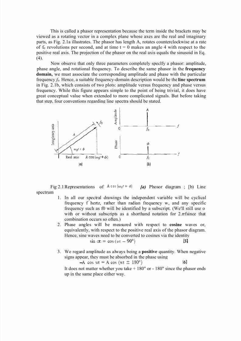
This is called a phasor representation because the term inside the brackets may be
viewed as a rotating vector in a complex plane whose axes are the real and imaginary
parts, as Fig. 2.1a illustrates. The phasor has length A, rotates counterclockwise at a rateof f 0 revolutions per second, and at time t = 0 makes an angle 4 with respect to the
positive real axis. The projection of the phasor on the real axis equals the sinusoid in Eq.
(4). Now observe that only three parameters completely speclfy a phasor: amplitude,
phase angle, and rotational frequency. To describe the same phasor in the frequencydomain, we must associate the corresponding amplitude and phase with the particular frequency f 0. Hence, a suitable frequency-domain description would be the line spectrumin Fig. 2.1b, which consists of two plots: amplitude versus frequency and phase versus
frequency. While this figure appears simple to the point of being trivial, it does have
great conceptual value when extended to more complicated signals. But before takingthat step, four conventions regarding line spectra should be stated.
Fig 2.1Representations of [a) Phosor diagram ; [b) Line
spectrum
1. In all our spectral drawings the independent variable will be cyclicalfrequency f hertz, rather than radian frequency w, and any specific
frequency such as f0 will be identified by a subscript. (We'll still use o
with or without subscripts as a shorthand notation for 2.rrfsince that
combination occurs so often.)2. Phase angles will be measured with respect to cosine waves or,
equivalently, with respect to the positive real axis of the phasor diagram.
Hence, sine waves need to be converted to cosines via the identity
3. We regard amplitude as always being a positive quantity. When negativesigns appear, they must be absorbed in the phase using
It does not matter whether you take + 180" or - 180" since the phasor ends
up in the same place either way.

8/8/2019 PSTS 23344
http://slidepdf.com/reader/full/psts-23344 6/67
4. Phase angles usually are expressed in degrees even though other angles
such as wt are inherently in radians. No confusion should result from this
mixed notation since angles expressed in degrees will always carry theappropriate symbol.
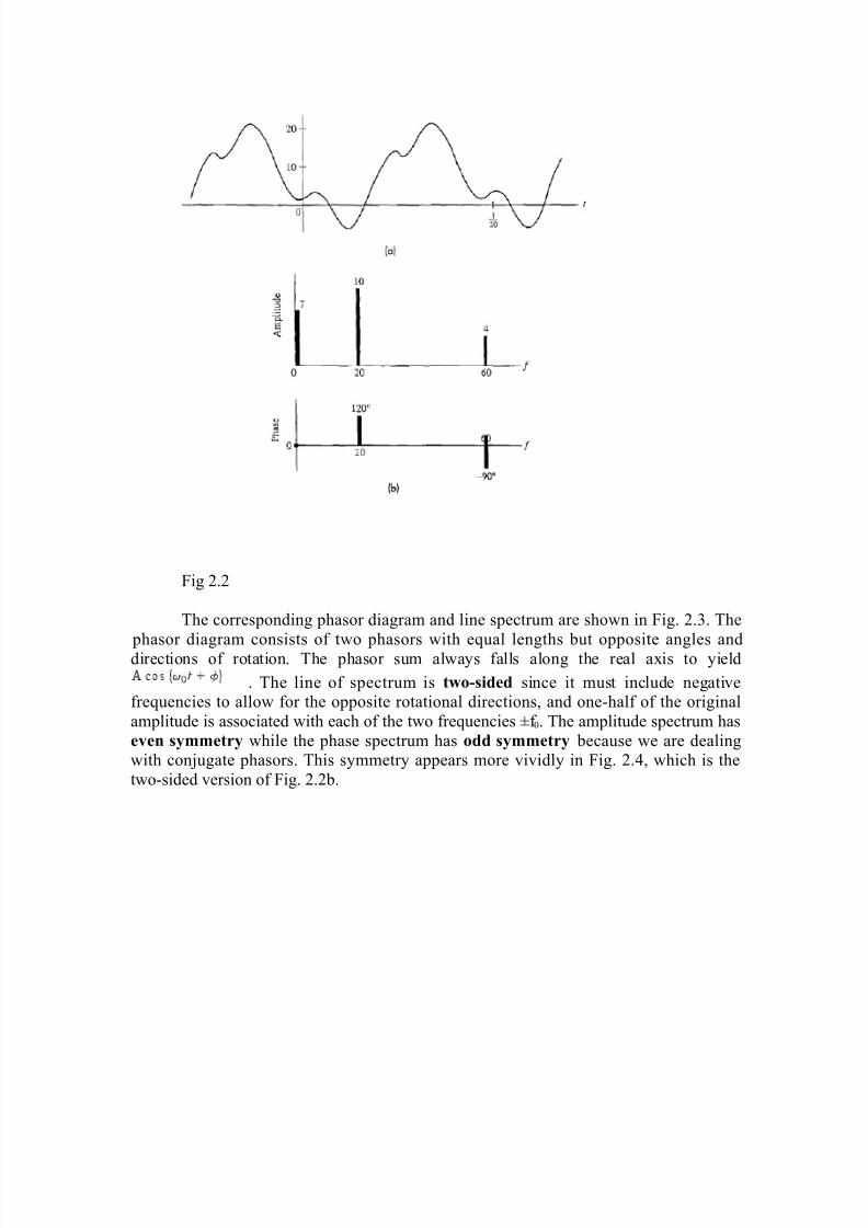
To illustrate these conventions and to carry further the idea of line spectrum,
consider the signal
which is sketched in Fig. 2.2a. Converting the constant term to a zero frequency or dc(direct-current) component and applying Eqs. (5) and (6) gives the sum of cosines
whose spectrum is shown in Fig. 2.2b.
Drawings like Fig. 2.2b, called one-sided or positive-frequency line spectra, can be constructed for any linear combination of sinusoids. But another spectral
representation turns out to be more valuable, even though it involves negativefrequencies. We obtain this representation from Eq. (4) by recalling that
, where z is any complex quantity with complex conjugate z*.
Hence, if then and Eq.(4) becomes
so we now have a pair of conjugate phasors.
8/8/2019 PSTS 23344
http://slidepdf.com/reader/full/psts-23344 7/67
Fig 2.2
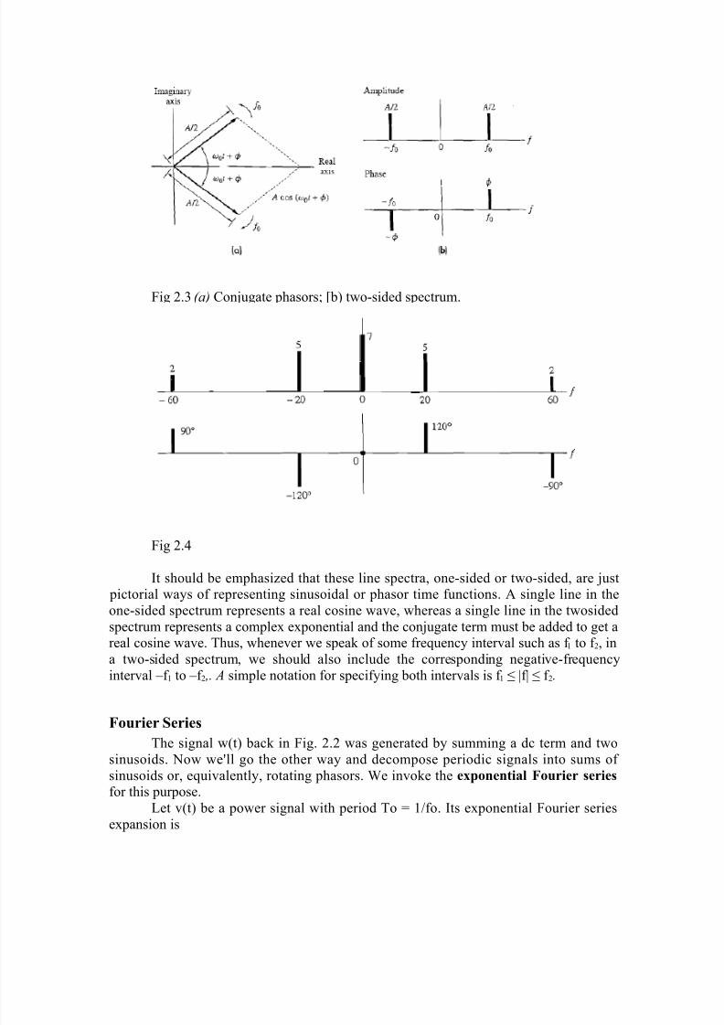
The corresponding phasor diagram and line spectrum are shown in Fig. 2.3. The
phasor diagram consists of two phasors with equal lengths but opposite angles anddirections of rotation. The phasor sum always falls along the real axis to yield
. The line of spectrum is two-sided since it must include negativefrequencies to allow for the opposite rotational directions, and one-half of the original
amplitude is associated with each of the two frequencies ±f 0. The amplitude spectrum haseven symmetry while the phase spectrum has odd symmetry because we are dealingwith conjugate phasors. This symmetry appears more vividly in Fig. 2.4, which is the
two-sided version of Fig. 2.2b.
8/8/2019 PSTS 23344
http://slidepdf.com/reader/full/psts-23344 8/67
Fig 2.3 (a) Conjugate phasors; [b) two-sided spectrum.
Fig 2.4
It should be emphasized that these line spectra, one-sided or two-sided, are just pictorial ways of representing sinusoidal or phasor time functions. A single line in the
one-sided spectrum represents a real cosine wave, whereas a single line in the twosided
spectrum represents a complex exponential and the conjugate term must be added to get areal cosine wave. Thus, whenever we speak of some frequency interval such as f 1 to f 2, in
a two-sided spectrum, we should also include the corresponding negative-frequency
interval –f 1 to –f 2 ,. A simple notation for specifying both intervals is f 1 ≤ |f| ≤ f 2.
Fourier SeriesThe signal w(t) back in Fig. 2.2 was generated by summing a dc term and two
sinusoids. Now we'll go the other way and decompose periodic signals into sums of
sinusoids or, equivalently, rotating phasors. We invoke the exponential Fourier seriesfor this purpose.
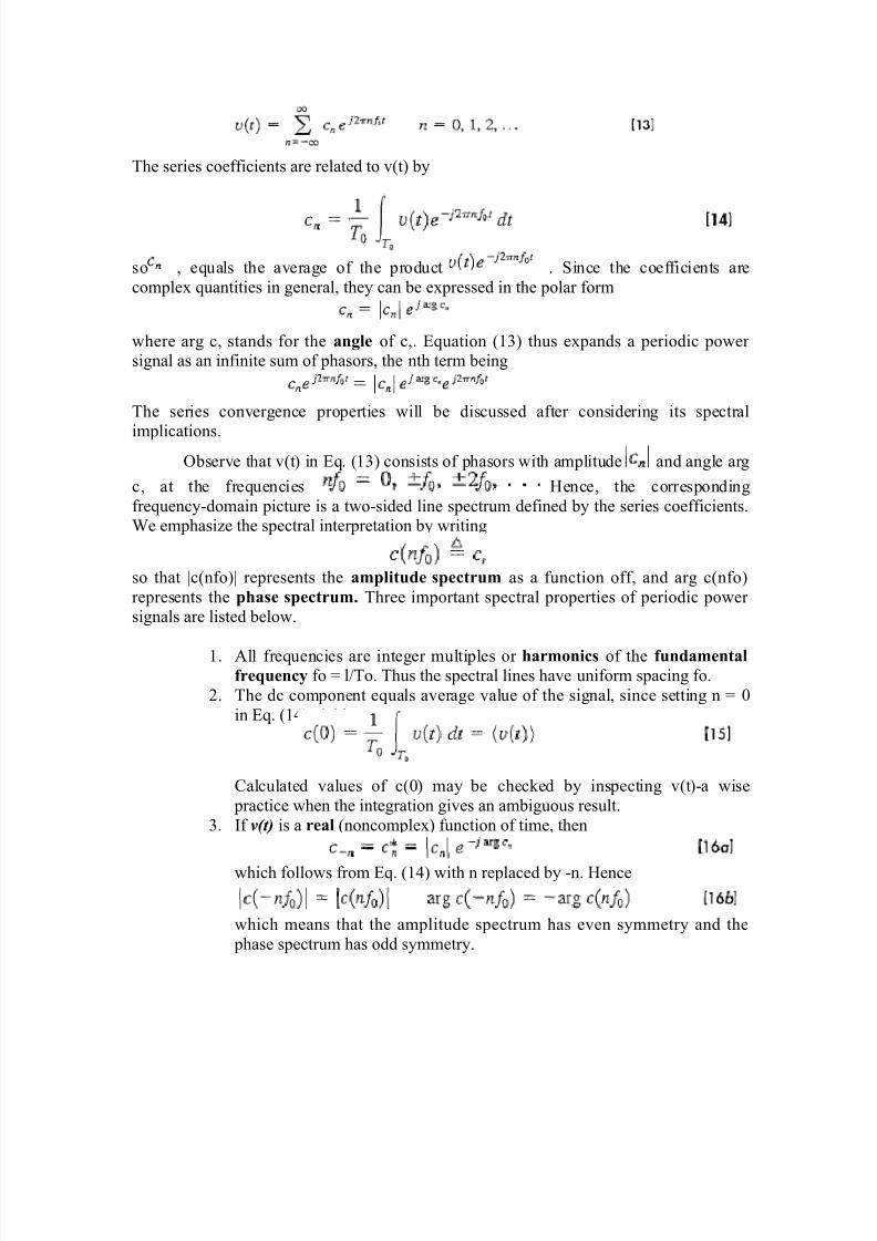
Let v(t) be a power signal with period To = 1/fo. Its exponential Fourier series
expansion is
8/8/2019 PSTS 23344
http://slidepdf.com/reader/full/psts-23344 9/67
The series coefficients are related to v(t) by
so , equals the average of the product . Since the coefficients are
complex quantities in general, they can be expressed in the polar form
where arg c, stands for the angle of c,. Equation (13) thus expands a periodic power signal as an infinite sum of phasors, the nth term being
The series convergence properties will be discussed after considering its spectral
implications.
Observe that v(t) in Eq. (13) consists of phasors with amplitude and angle arg
c, at the frequencies Hence, the corresponding
frequency-domain picture is a two-sided line spectrum defined by the series coefficients.We emphasize the spectral interpretation by writing
so that |c(nfo)| represents the amplitude spectrum as a function off, and arg c(nfo)
represents the phase spectrum. Three important spectral properties of periodic power signals are listed below.
1. All frequencies are integer multiples or harmonics of the fundamentalfrequency fo = l/To. Thus the spectral lines have uniform spacing fo.
2. The dc component equals average value of the signal, since setting n = 0
in Eq. (14) yields
Calculated values of c(0) may be checked by inspecting v(t)-a wise
practice when the integration gives an ambiguous result.
3. If v(t) is a real (noncomplex) function of time, then
which follows from Eq. (14) with n replaced by -n. Hence
which means that the amplitude spectrum has even symmetry and the
phase spectrum has odd symmetry.
8/8/2019 PSTS 23344
http://slidepdf.com/reader/full/psts-23344 10/67
When dealing with real signals, the property in Eq. (16) allows us to regroup the
exponential series into complex-conjugate pairs, except for c0. Equation (13) then
becomes
which is the trigonometric Fourier series and suggests a one-sided spectrum.Most of the time, however, we'll use the exponential series and two-sided spectra.
One final comment should be made before taking up an example. The integration
for often involves a phasor average in the form
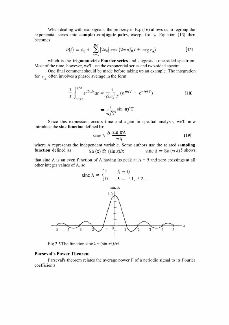
Since this expression occurs time and again in spectral analysis, we'll now
introduce the sinc function defined by
where A represents the independent variable. Some authors use the related samplingfunction defined as so that . Figure 2.5 shows
that sinc A is an even function of A having its peak at A = 0 and zero crossings at all
other integer values of A, so
Fig 2.5The function sinc λ = (sin πλ)/πλ
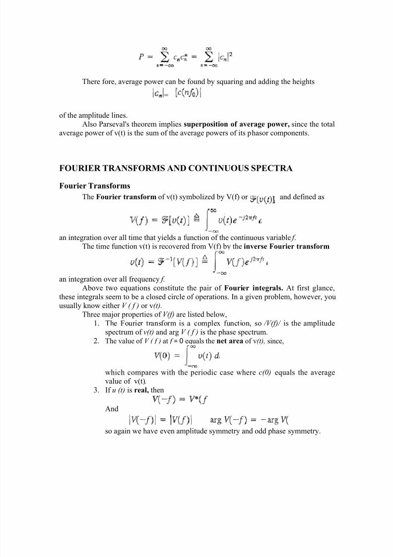
Parseval's Power TheoremParseval's theorem relates the average power P of a periodic signal to its Fourier
coefficients
8/8/2019 PSTS 23344
http://slidepdf.com/reader/full/psts-23344 11/67
There fore, average power can be found by squaring and adding the heights
=
of the amplitude lines.
Also Parseval's theorem implies superposition of average power, since the totalaverage power of v(t) is the sum of the average powers of its phasor components.
FOURIER TRANSFORMS AND CONTINUOUS SPECTRA
Fourier Transforms
The Fourier transform of v(t) symbolized by V(f) or and defined as
an integration over all time that yields a function of the continuous variable f .The time function v(t) is recovered from V(f) by the inverse Fourier transform
an integration over all frequency f.
Above two equations constitute the pair of Fourier integrals. At first glance,
these integrals seem to be a closed circle of operations. In a given problem, however, you
usually know either V ( f ) or v(t).
Three major properties of V(f) are listed below,
1. The Fourier transform is a complex function, so /V(f)/ is the amplitude
spectrum of v(t) and arg V ( f ) is the phase spectrum.2. The value of V ( f ) at f = 0 equals the net area of v(t), since,
which compares with the periodic case where c(0) equals the averagevalue of v(t).
3. If u (t) is real, then
And
so again we have even amplitude symmetry and odd phase symmetry.
8/8/2019 PSTS 23344
http://slidepdf.com/reader/full/psts-23344 12/67
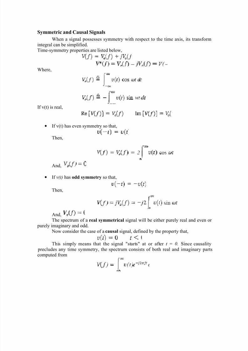
Symmetric and Causal SignalsWhen a signal possesses symmetry with respect to the time axis, its transform
integral can be simplified.Time-symmetry properties are listed below,
Where,
If v(t) is real,
• If v(t) has even symmetry so that,
Then,
And,
• If v(t) has odd symmetry so that,
Then,
And,The spectrum of a real symmetrical signal will be either purely real and even or
purely imaginary and odd.
Now consider the case of a causal signal, defined by the property that,
This simply means that the signal "starts" at or after t = 0. Since causality precludes any time symmetry, the spectrum consists of both real and imaginary partscomputed from
8/8/2019 PSTS 23344
http://slidepdf.com/reader/full/psts-23344 13/67
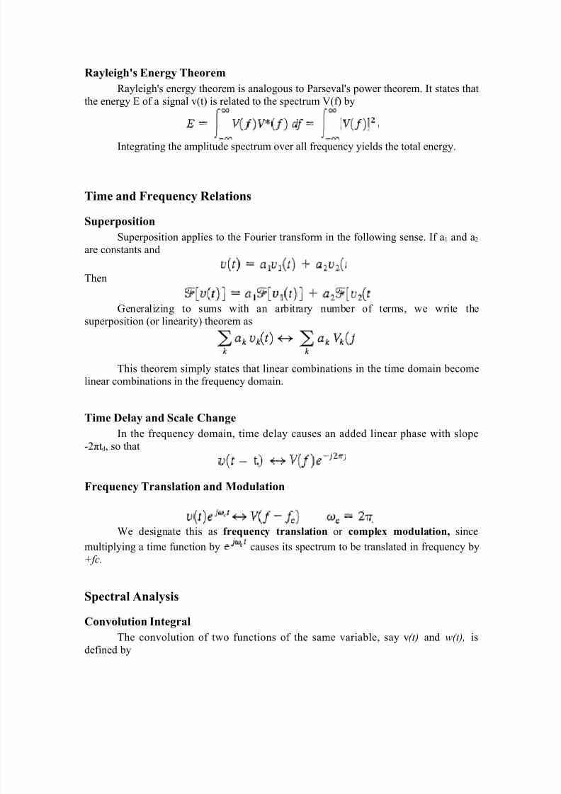
Rayleigh's Energy TheoremRayleigh's energy theorem is analogous to Parseval's power theorem. It states that
the energy E of a signal v(t) is related to the spectrum V(f) by
Integrating the amplitude spectrum over all frequency yields the total energy.
Time and Frequency Relations
SuperpositionSuperposition applies to the Fourier transform in the following sense. If a1 and a2
are constants and
Then
Generalizing to sums with an arbitrary number of terms, we write the
superposition (or linearity) theorem as
This theorem simply states that linear combinations in the time domain become
linear combinations in the frequency domain.
Time Delay and Scale ChangeIn the frequency domain, time delay causes an added linear phase with slope
-2πtd, so that
Frequency Translation and Modulation
We designate this as frequency translation or complex modulation, since
multiplying a time function by causes its spectrum to be translated in frequency by
+fc.
Spectral Analysis
Convolution IntegralThe convolution of two functions of the same variable, say v(t) and w(t), is
defined by

8/8/2019 PSTS 23344
http://slidepdf.com/reader/full/psts-23344 14/67
Convolution TheoremsConvolution is commutative, associative and distributive. These properties are
listed below along with their properties.
Having defined and examined the convolution operation, we now list the twoconvolution theorems:
Dirac Delta FunctionThe Dirac Delta function, often referred to as the unit impulse or delta function, is
the function that defines the idea of a unit impulse. This function is one that isinfinitesimally narrow, infinitely tall, yet integrates to unity, one. The impulse function is
often written as δ(t).
Step and Signum Functions• Unit step function
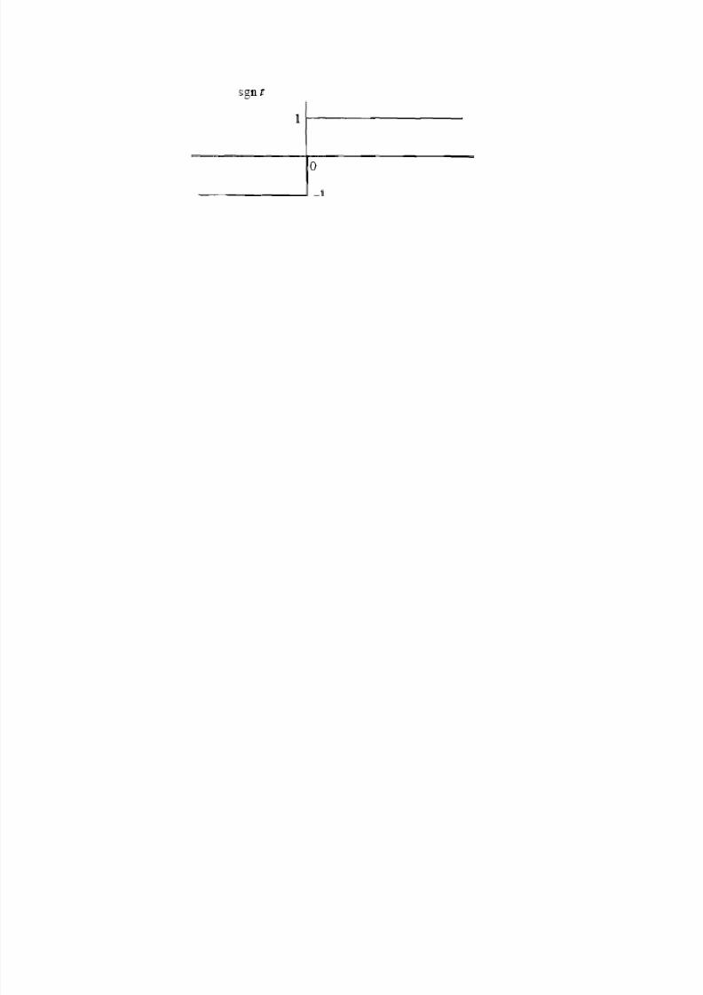
• Signum function
8/8/2019 PSTS 23344
http://slidepdf.com/reader/full/psts-23344 15/67
8/8/2019 PSTS 23344
http://slidepdf.com/reader/full/psts-23344 16/67
Chapter 3
Signal Transmission and Filtering
LTI SystemA system is linear if it has the following two properties:
1. Superposition: If and then
2. Scaling: If , then for a constant a ,
A system is time invariant if for any ,
If a system that is both linear and time-invariant, we call it a LTI system. Notethat the properties are independent of each other - one may have a linear time-varying
system or a non-linear time invariant system.
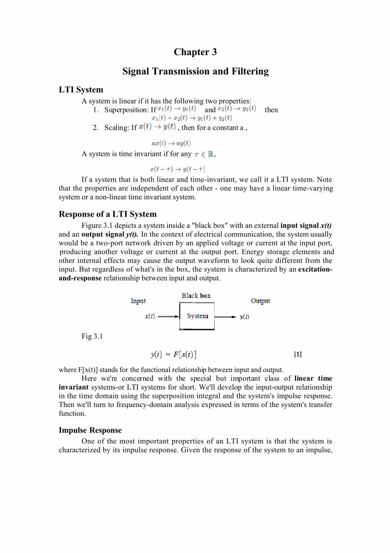
Response of a LTI SystemFigure 3.1 depicts a system inside a "black box" with an external input signal x(t)
and an output signal y(t). In the context of electrical communication, the system usuallywould be a two-port network driven by an applied voltage or current at the input port,
producing another voltage or current at the output port. Energy storage elements and
other internal effects may cause the output waveform to look quite different from theinput. But regardless of what's in the box, the system is characterized by an excitation-and-response relationship between input and output.
Fig 3.1
where F[x(t)] stands for the functional relationship between input and output.
Here we're concerned with the special but important class of linear time
invariant systems-or LTI systems for short. We'll develop the input-output relationshipin the time domain using the superposition integral and the system's impulse response.
Then we'll turn to frequency-domain analysis expressed in terms of the system's transfer
function.
Impulse ResponseOne of the most important properties of an LTI system is that the system is
characterized by its impulse response. Given the response of the system to an impulse,

8/8/2019 PSTS 23344
http://slidepdf.com/reader/full/psts-23344 17/67
the response to any other signal can be computed in a straightforward manner. As the
name suggests the impulse response is the response of a system given an impulse. All
systems have this, but only in LTI systems does this allow us to characterize the responseto other input signals using this.
Step ResponseWhen x(t) = u(t) we can calculate the system's step response,
This derivative relation between the impulse and step response follows from the
general convolution property
Thus, since g(t) = h (t)* u(t)
Superposition IntegralSuperposition integral expresses the forced response as a convolution of the
input x(t) with the impulse response h(t). System analysis in the time domain therefore
requires knowledge of the impulse response along with the ability to carry out theconvolution.
Transfer Functions and Frequency ResponseTime-domain analysis becomes increasingly difficult for higher-order systems,
and the mathematical complications tend to obscure significant points. We'll gain adifferent and often clearer view of system response by going to the frequency domain. As
a first step in this direction, we define the system transfer function to be the Fourier transform of the impulse response, namely,
• When h(t) is a real time function, H(f) has the hermitian symmetry,
8/8/2019 PSTS 23344
http://slidepdf.com/reader/full/psts-23344 18/67
So that,
represents the system's amplitude ratio as a function of frequency
(sometimes called the amplitude response or gain). By the same token, arg H(f)represents the phase shift. Plots of and arg H(f) versus frequency give us the
frequency-domain representation of the system or, equivalently, the system's frequency
response. Henceforth, we'll refer to H(f) as either the transfer function or frequency-response function.
Now let x(t) be any signal with spectrum X(f). Calling upon the convolution
theorem, we take the transform of y(t) = h(t)* x(t) to obtain
This elegantly simple result constitutes the basis of frequency-domain system
analysis. It says that, the output spectrum Y(f) equals to input spectrum X(f) multiplied
by transfer function H(f).The corresponding amplitude and phase spectra are,
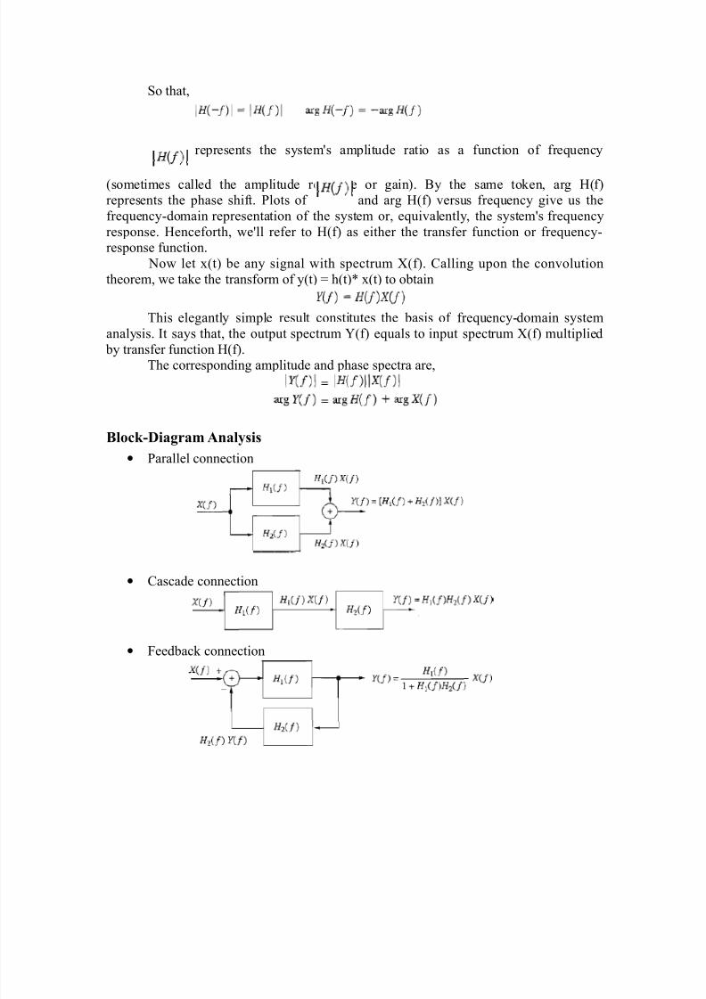
Block-Diagram Analysis• Parallel connection
• Cascade connection
• Feedback connection
8/8/2019 PSTS 23344
http://slidepdf.com/reader/full/psts-23344 19/67
Signal Distortion in Transmission
Distortionless TransmissionDistortionless transmission means that the output signal has the same "shape" as
the input. More precisely, given an input signal x(t), we say that the output signal is
distorted if it differs from input only by a multiplying constant and finite time delay.Analytically, we have distortionless transmission if,
where K and td are constants.
The properties of a distortionless system are easily found by examining the output
spectrum
Now by definition of transfer function, Y(f ) = H(f )X(f ), so
Linear DistortionLinear distortion includes any amplitude or delay distortion associated with a
linear transmission system. Amplitude distortion is easily described .in the frequency
domain; it means simply that the output frequency components are not in correct
proportion. Since this is caused by | H(f )|not being constant with frequency, amplitudedistortion is sometimes called frequency distortion.
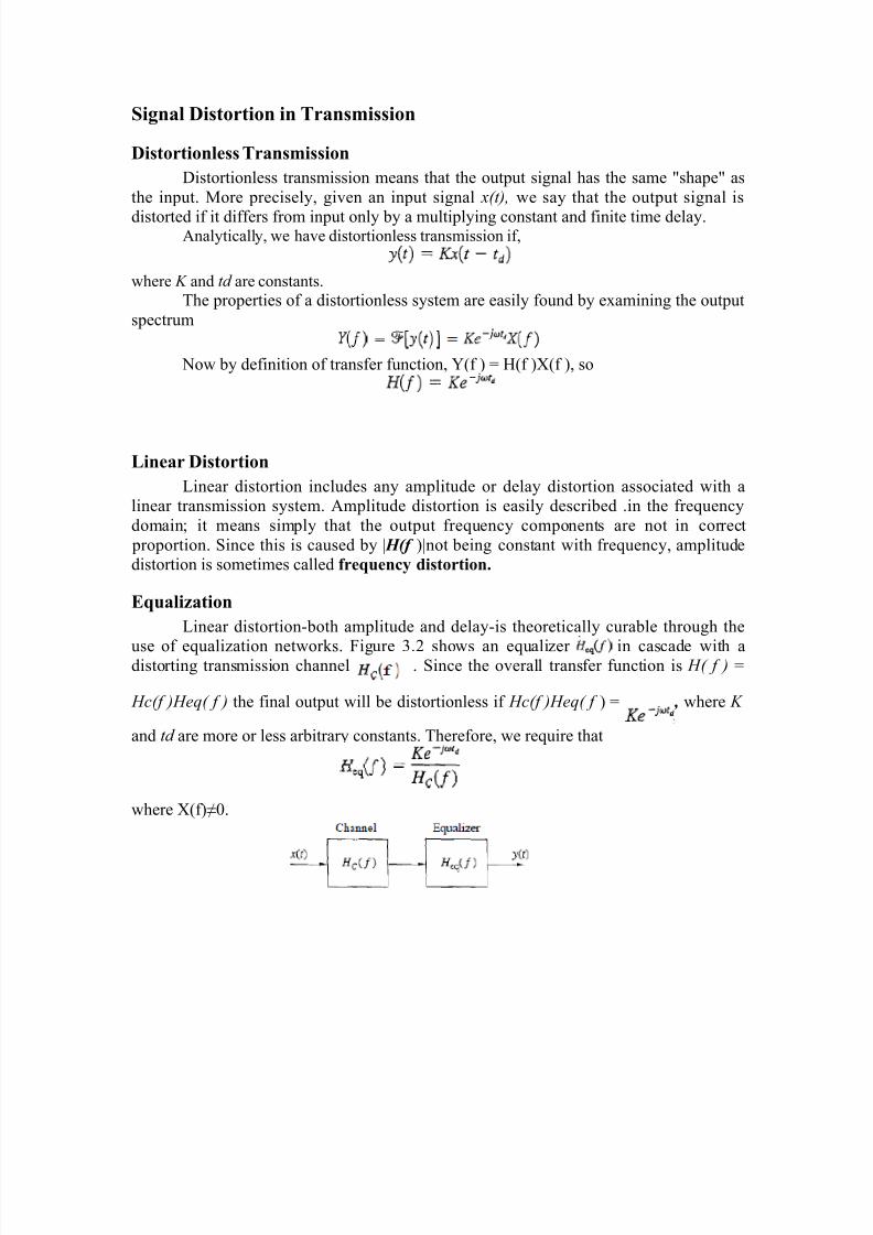
EqualizationLinear distortion-both amplitude and delay-is theoretically curable through the
use of equalization networks. Figure 3.2 shows an equalizer in cascade with adistorting transmission channel . Since the overall transfer function is H( f ) =
Hc(f )Heq( f ) the final output will be distortionless if Hc(f )Heq( f ) = , where K
and td are more or less arbitrary constants. Therefore, we require that
where X(f)≠0.
8/8/2019 PSTS 23344
http://slidepdf.com/reader/full/psts-23344 20/67
Transmission Loss
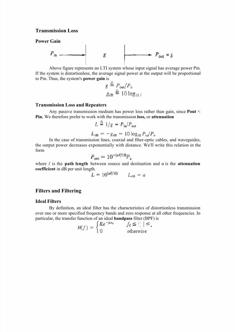
Power Gain
Above figure represents an LTI system whose input signal has average power Pin.If the system is distortionless, the average signal power at the output will be proportional
to Pin. Thus, the system's power gain is
Transmission Loss and RepeatersAny passive transmission medium has power loss rather than gain, since Pout <
Pin. We therefore prefer to work with the transmission loss, or attenuation
In the case of transmission lines, coaxial and fiber-optic cables, and waveguides,
the output power decreases exponentially with distance. We'll write this relation in theform
where l is the path length between source and destination and α is the attenuationcoefficient in dB per unit length.
Filters and Filtering
Ideal FiltersBy definition, an ideal filter has the characteristics of distortionless transmission
over one or more specified frequency bands and zero response at all other frequencies. In particular, the transfer function of an ideal bandpass filter (BPF) is

8/8/2019 PSTS 23344
http://slidepdf.com/reader/full/psts-23344 21/67
The parameters f l and fu are the lower and upper cutoff frequencies, respectively,
since they mark the end points of the passband. The filter's bandwidth is
which we measure in terms of the positive-frequency portion of the passband.
In similar fashion, an ideal lowpass filter (LPF) is defined with f l = 0, so B =fuwhile an ideal highpass filter (HPF) has f l > 0 and fu = α. Ideal band-rejection or notchfilters provide distortionless transmission over all frequencies except some stopband, say
, where H( f ) = 0.
But all such filters are physically unrealizable in the sense that their
characteristics cannot be achieved with a finite number of elements. We'll slup thegeneral proof of this assertion. Instead, we'll give an instructive plausibility argument
based on the impulse response.
Ideal lowpass filter. (a) Transfer function; (b) impulse response.
Transfer function of ideal low pass filter,
Its impulse response will be,
8/8/2019 PSTS 23344
http://slidepdf.com/reader/full/psts-23344 22/67
Correlation and Spectral DensityCorrelation focuses on time averages and signal power or energy. Taking the
Fourier transform of a correlation function leads to frequency-domain representation in
terms of spectral density functions, equivalent to energy spectral density in the case of an energy signal. In the case of a power signal, the spectral density function tells us the
power distribution over frequency.
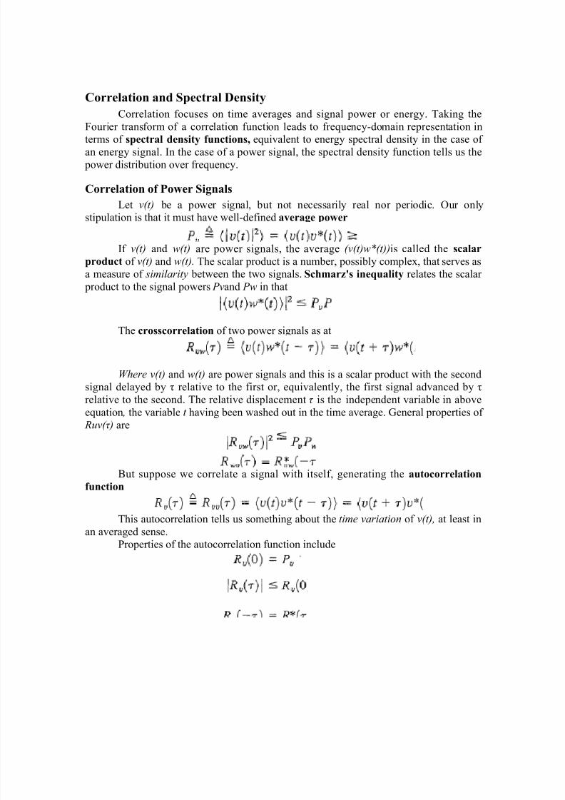
Correlation of Power SignalsLet v(t) be a power signal, but not necessarily real nor periodic. Our only
stipulation is that it must have well-defined average power
If v(t) and w(t) are power signals, the average (v(t)w*(t))is called the scalarproduct of v(t) and w(t). The scalar product is a number, possibly complex, that serves asa measure of similarity between the two signals. Schmarz's inequality relates the scalar
product to the signal powers Pvand Pw in that
The crosscorrelation of two power signals as at
Where v(t) and w(t) are power signals and this is a scalar product with the secondsignal delayed by τ relative to the first or, equivalently, the first signal advanced by τ
relative to the second. The relative displacement τ is the independent variable in above
equation , the variable t having been washed out in the time average. General properties of Ruv(τ) are
But suppose we correlate a signal with itself, generating the autocorrelationfunction
This autocorrelation tells us something about the time variation of v(t), at least in
an averaged sense.Properties of the autocorrelation function include

8/8/2019 PSTS 23344
http://slidepdf.com/reader/full/psts-23344 23/67
Correlation of Energy SignalsAveraging products of energy signals over all time yields zero. But we can
meaningfully speak of the total energy
Similarly, the correlation functions for energy signals can be defined as
Since the integration operation has the same mathematical properties as
the time-average operation , all of our previous correlation relations hold for the
case of energy signals if we replace average power P, with total energy E,. Thus, for
instance, we have the property
Spectral Density FunctionsAt last we're prepared to discuss spectral density functions. Given a power or
energy signal v(t), its spectral density function Gv(f) represents the distribution of power or energy in the frequency domain and has two essential properties. First, the area under
Gv(f) equals the average power or total energy, so
Second, if x(t) is the input to an LTI system with then the input
and output spectral density functions are related by
Since is the power or energy gain at any f. These two properties are
combined in
which expresses the output power or energy Ry(0) in terms of the input spectral density.
8/8/2019 PSTS 23344
http://slidepdf.com/reader/full/psts-23344 24/67
Chapter 4
Modulation and Frequency ConversionContinuous-wave Modulation
• Amplitude Modulation, the amplitude of sinusoidal carrier is varied with incoming message signal.
• Angle Modulation, the instantaneous frequency or phase of
sinusoidal carrier is varied with the message signal.
Communication channel requires a shift of the range of baseband frequencies into
other frequency ranges suitable for transmission, and a corresponding shift back to the
original frequency range after reception.A shift of the range of frequencies in a signal is accomplished by using
modulation, by which some characteristic of a carrier is varied in accordance with a
modulating signal. Modulation is performed at the transmitting end of the communicationsystem. At the receiving end, the original baseband signal is restored by the process of
demodulation, which is the reverse of the modulation process.
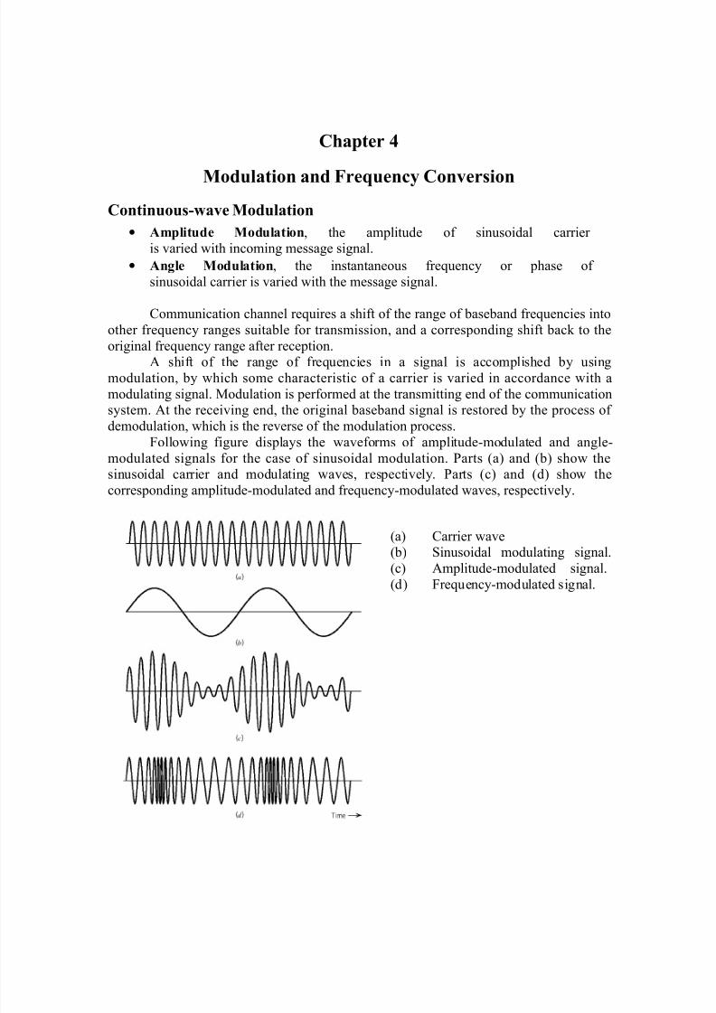
Following figure displays the waveforms of amplitude-modulated and angle-
modulated signals for the case of sinusoidal modulation. Parts (a) and (b) show thesinusoidal carrier and modulating waves, respectively. Parts (c) and (d) show the
corresponding amplitude-modulated and frequency-modulated waves, respectively.
(a) Carrier wave(b) Sinusoidal modulating signal.
(c) Amplitude-modulated signal.
(d) Frequency-modulated signal.
8/8/2019 PSTS 23344
http://slidepdf.com/reader/full/psts-23344 25/67
Amplitude Modulation
Consider a sinusoidal carrier wave c(t ) defined byc(t ) = Ac cos(2π f ct )
where Ac is the carrier amplitude and f c is the carrier frequency. Let m(t) denote the
baseband signal and the carrier wave c(t) is physically independent of the message signalm(t). An amplitude-modulated (AM) wave can be described as:
s(t ) = Ac [1 + k am(t )] cos(2π f ct )
where k a is the amplitude sensitivity of the modulator responsible for the generation of
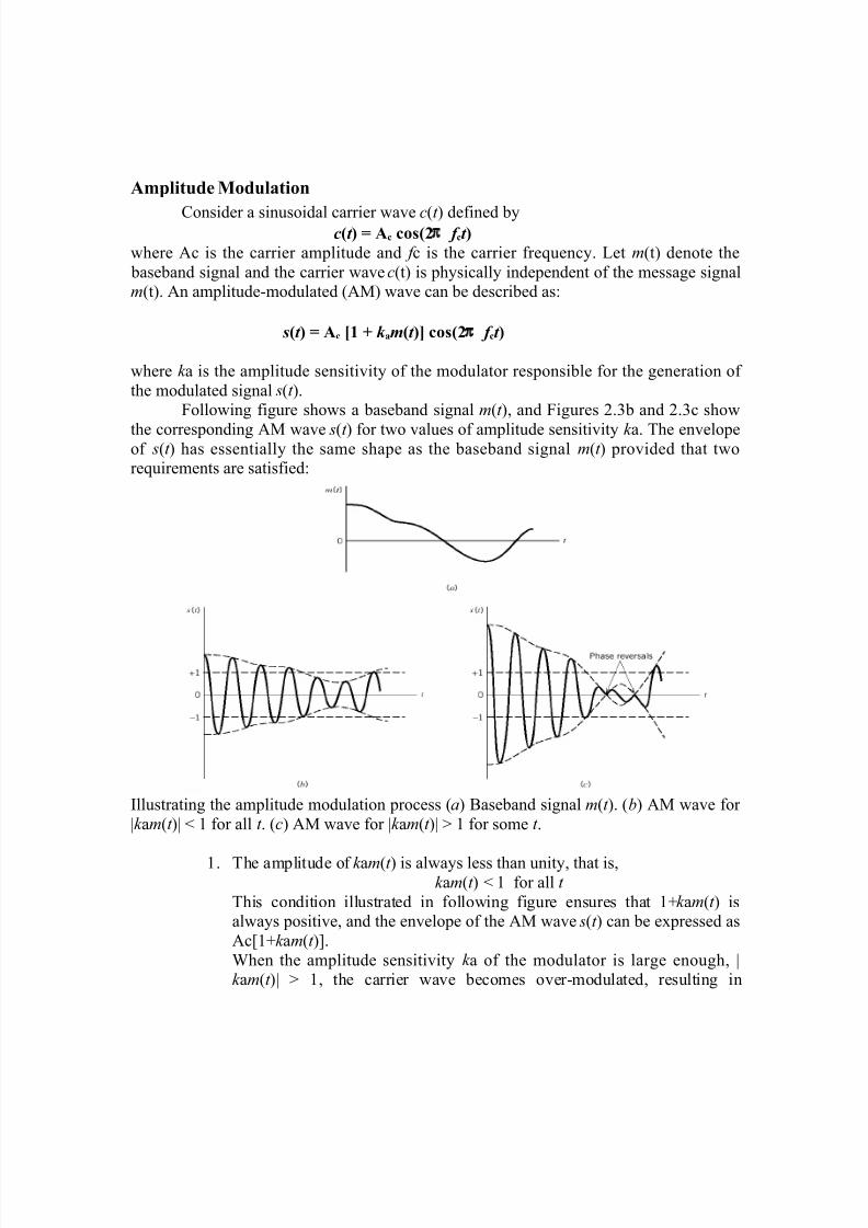
the modulated signal s(t ).Following figure shows a baseband signal m(t ), and Figures 2.3b and 2.3c show
the corresponding AM wave s(t ) for two values of amplitude sensitivity k a. The envelopeof s(t ) has essentially the same shape as the baseband signal m(t ) provided that tworequirements are satisfied:
Illustrating the amplitude modulation process (a) Baseband signal m(t ). (b) AM wave for
|k am(t )| < 1 for all t . (c) AM wave for |k am(t )| > 1 for some t .
1. The amplitude of k am(t ) is always less than unity, that is, k am(t ) < 1 for all t
This condition illustrated in following figure ensures that 1+k am(t ) isalways positive, and the envelope of the AM wave s(t ) can be expressed as
Ac[1+k am(t )].
When the amplitude sensitivity k a of the modulator is large enough, |k am(t )| > 1, the carrier wave becomes over-modulated, resulting in
8/8/2019 PSTS 23344
http://slidepdf.com/reader/full/psts-23344 26/67
carrier phase reversals whenever the factor 1+k am(t ) crosses zero. The
modulated wave then exhibits envelope distortion.
2. The carrier frequency f c is much greater than the highest frequency
component W of the message signal m(t ), that is
f c >> W We call W the message bandwidth. If the above condition is not satisfied,
an envelope cannot be detected satisfactorily.
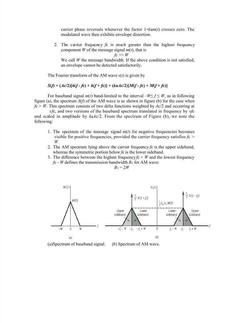
The Fourier transform of the AM wave s(t ) is given by
S ( f ) = ( Ac/2)[δ( f - f c) + δ( f + f c)] + (k a Ac/2)[ M ( f - f c) + M ( f + f c)]
For baseband signal m(t ) band-limited to the interval – W ≤ f ≤ W , as in following
figure (a), the spectrum S ( f ) of the AM wave is as shown in figure (b) for the case when f c > W . This spectrum consists of two delta functions weighted by Ac/2 and occurring at
± f c, and two versions of the baseband spectrum translated in frequency by ± f cand scaled in amplitude by k a Ac/2. From the spectrum of Figure (b), we note the
following:
1. The spectrum of the message signal m(t ) for negative frequencies becomes
visible for positive frequencies, provided the carrier frequency satisfies f c >W .
2. The AM spectrum lying above the carrier frequency f c is the upper sideband,
whereas the symmetric portion below f c is the lower sideband.
3. The difference between the highest frequency f c + W and the lowest frequency f c - W defines the transmission bandwidth BT for AM wave:
BT = 2W
(a)Spectrum of baseband signal. (b) Spectrum of AM wave.

8/8/2019 PSTS 23344
http://slidepdf.com/reader/full/psts-23344 27/67
AM VIRTUES AND LIMITATIONS• In the transmitter, AM is accomplished using a nonlinear device. Fourier
analysis of the voltage developed across resistive load reveals the AMcomponents, which may be extracted by means of a BPF.
• In the receiver, AM demodulation is accomplished usinga nonlinear
device. The demodulator output developed across the load resistor isnearly the same as the envelope of the incoming AM wave, hence the
name "envelope detector."
Amplitude modulation suffers from two major limitations:1. AM is wasteful of power. The carrier wave c(t ) is independent of the
information signal m(t ). Only a fraction of the total transmitted power is
actually affected by m(t ).2. AM is wasteful of bandwidth. The upper and lower sidebands of an AM
wave are related by their symmetry about the carrier. Only one sideband is
necessary, and the communication channel needs to provide only the same
bandwidth as the baseband signal.
Linear Modulation SchemesIn its most general form, linear modulation is defined by
where SI(t ) is the in-phase component and S Q(t ) the quadrature component of the
modulated wave s(t). In linear modulation, both sI(t ) and sQ(t ) are low-pass signals thatare linearly related to the message signal m(t ).
Depending on sI(t ) and sQ(t ), three types of linear modulation are defined:
1. DSB modulation, where only the upper and lower sidebands are transmitted.2. SSB modulation, where only the lower or the upper sideband is transmitted.3. VSB modulation, where only a vestige of one of the sidebands and a modified
version of the other sideband are transmitted.
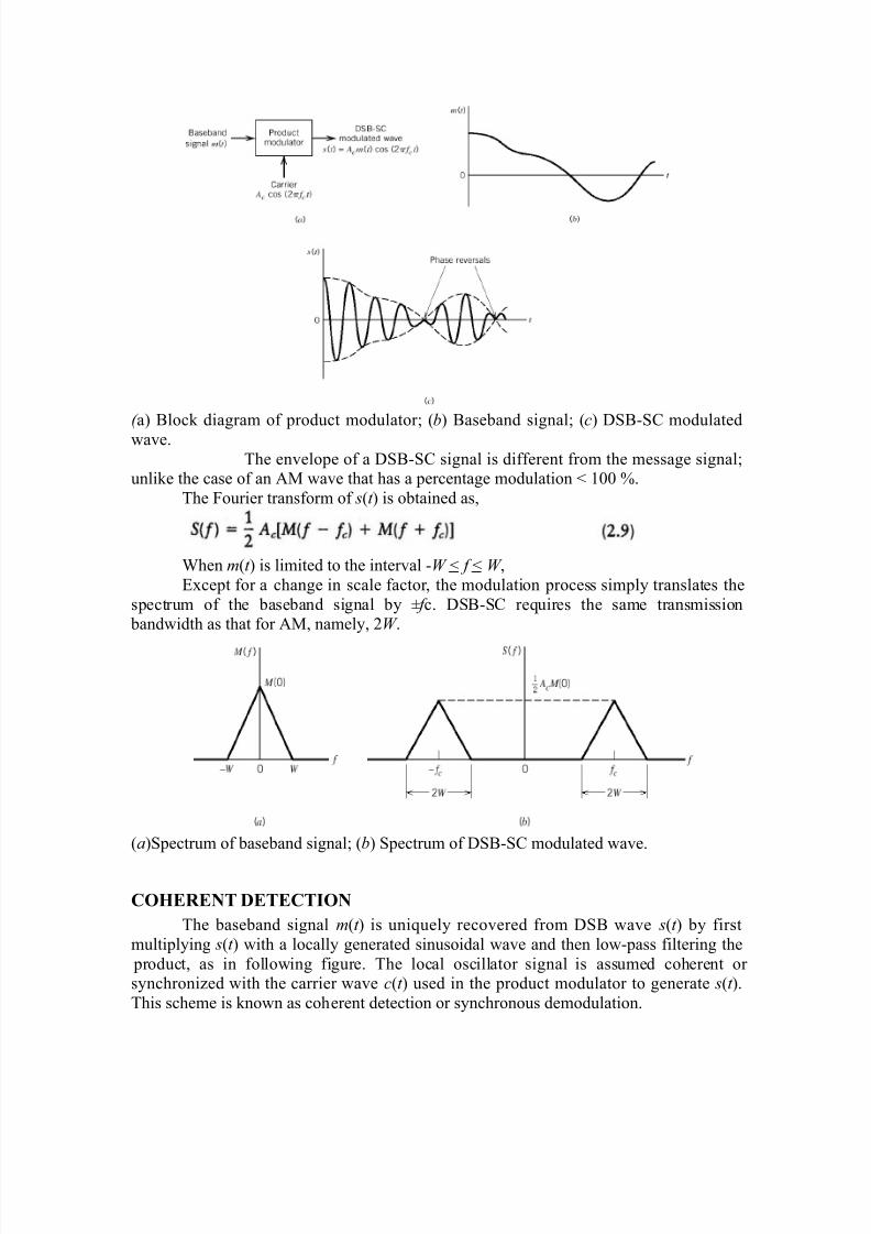
DSB-SC MODULATIONDSB-SC modulation is generated by using a product modulator that simply
multiplies the message signal m(t ) by the carrier wave Accos(2π f ct ), as illustrated in
following figure,
Specifically, we write
s(t ) = Acm(t ) cos(2π f ct )The modulated signal s(t ) undergoes a phase reversal whenever the message
signal m(t ) crosses zero.
8/8/2019 PSTS 23344
http://slidepdf.com/reader/full/psts-23344 28/67
( a) Block diagram of product modulator; (b) Baseband signal; (c) DSB-SC modulated
wave.
The envelope of a DSB-SC signal is different from the message signal;unlike the case of an AM wave that has a percentage modulation < 100 %.
The Fourier transform of s(t ) is obtained as,
When m(t ) is limited to the interval -W < f < W ,
Except for a change in scale factor, the modulation process simply translates the
spectrum of the baseband signal by ± f c. DSB-SC requires the same transmission bandwidth as that for AM, namely, 2W .
(a)Spectrum of baseband signal; (b) Spectrum of DSB-SC modulated wave.
COHERENT DETECTIONThe baseband signal m(t ) is uniquely recovered from DSB wave s(t ) by first
multiplying s(t ) with a locally generated sinusoidal wave and then low-pass filtering the
product, as in following figure. The local oscillator signal is assumed coherent or synchronized with the carrier wave c(t ) used in the product modulator to generate s(t ).
This scheme is known as coherent detection or synchronous demodulation.
8/8/2019 PSTS 23344
http://slidepdf.com/reader/full/psts-23344 29/67
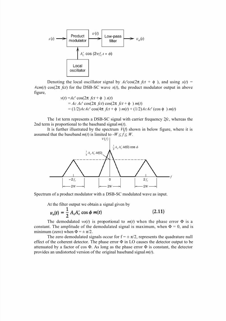
Denoting the local oscillator signal by Ac'cos(2π fct + φ ), and using s(t ) =
Acm(t ) cos(2π f ct ) for the DSB-SC wave s(t ), the product modulator output in above
figure,
v(t ) = Ac' cos(2π fct + φ ) s(t )
= Ac Ac' cos(2π fct ) cos(2π fct + φ ) m(t )
= (1/2) AcAc' cos(4π fct + φ ) m(t ) + (1/2) AcAc' (cos φ ) m(t )
The 1st term represents a DSB-SC signal with carrier frequency 2 fc, whereas the2nd term is proportional to the baseband signal m(t ).
It is further illustrated by the spectrum V ( f ) shown in below figure, where it is
assumed that the baseband m(t ) is limited to -W < f < W .
Spectrum of a product modulator with a DSB-SC modulated wave as input.
At the filter output we obtain a signal given by
The demodulated vo(t ) is proportional to m(t ) when the phase error Φ is a
constant. The amplitude of the demodulated signal is maximum, when Φ = 0, and isminimum (zero) when Φ = ± π/2.
The zero demodulated signals occur for f = ± π/2, represents the quadrature nulleffect of the coherent detector. The phase error Φ in LO causes the detector output to be
attenuated by a factor of cos Φ. As long as the phase error Φ is constant, the detector
provides an undistorted version of the original baseband signal m(t ).
8/8/2019 PSTS 23344
http://slidepdf.com/reader/full/psts-23344 30/67
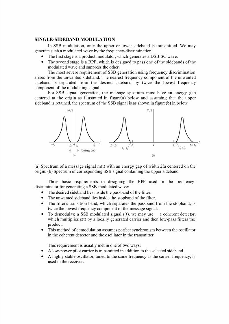
SINGLE-SIDEBAND MODULATIONIn SSB modulation, only the upper or lower sideband is transmitted. We may
generate such a modulated wave by the frequency-discrimination:
• The first stage is a product modulator, which generates a DSB-SC wave.• The second stage is a BPF, which is designed to pass one of the sidebands of the
modulated wave and suppress the other.The most severe requirement of SSB generation using frequency discrimination
arises from the unwanted sideband. The nearest frequency component of the unwanted
sideband is separated from the desired sideband by twice the lowest frequency
component of the modulating signal.For SSB signal generation, the message spectrum must have an energy gap
centered at the origin as illustrated in figure(a) below and assuming that the upper
sideband is retained, the spectrum of the SSB signal is as shown in figure(b) in below.
(a) Spectrum of a message signal m(t) with an energy gap of width 2fa centered on the
origin. (b) Spectrum of corresponding SSB signal containing the upper sideband.
Three basic requirements in designing the BPF used in the frequency-
discriminator for generating a SSB-modulated wave:
• The desired sideband lies inside the passband of the filter.
• The unwanted sideband lies inside the stopband of the filter.
• The filter's transition band, which separates the passband from the stopband, is
twice the lowest frequency component of the message signal.
• To demodulate a SSB modulated signal s(t), we may use a coherent detector,which multiplies s(t) by a locally generated carrier and then low-pass filters the
product.
• This method of demodulation assumes perfect synchronism between the oscillator
in the coherent detector and the oscillator in the transmitter.
This requirement is usually met in one of two ways:
• A low-power pilot carrier is transmitted in addition to the selected sideband.
• A highly stable oscillator, tuned to the same frequency as the carrier frequency, is
used in the receiver.
8/8/2019 PSTS 23344
http://slidepdf.com/reader/full/psts-23344 31/67
In the latter method, there would be some phase error Φ the local oscillator output
with respect to the carrier wave used to generate the SSB wave. The effect is to introduce
a phase distortion in the demodulated signal, where each frequency component of theoriginal message signal undergoes a phase shift Φ. This phase distortion is tolerable in
voice communications, because the human ear is relatively insensitive to phase distortion.
The presence of phase distortion gives rise to a Donald Duck voice effect. In thetransmission of music and video signals, the presence of this form of waveform distortion
is utterly unacceptable.
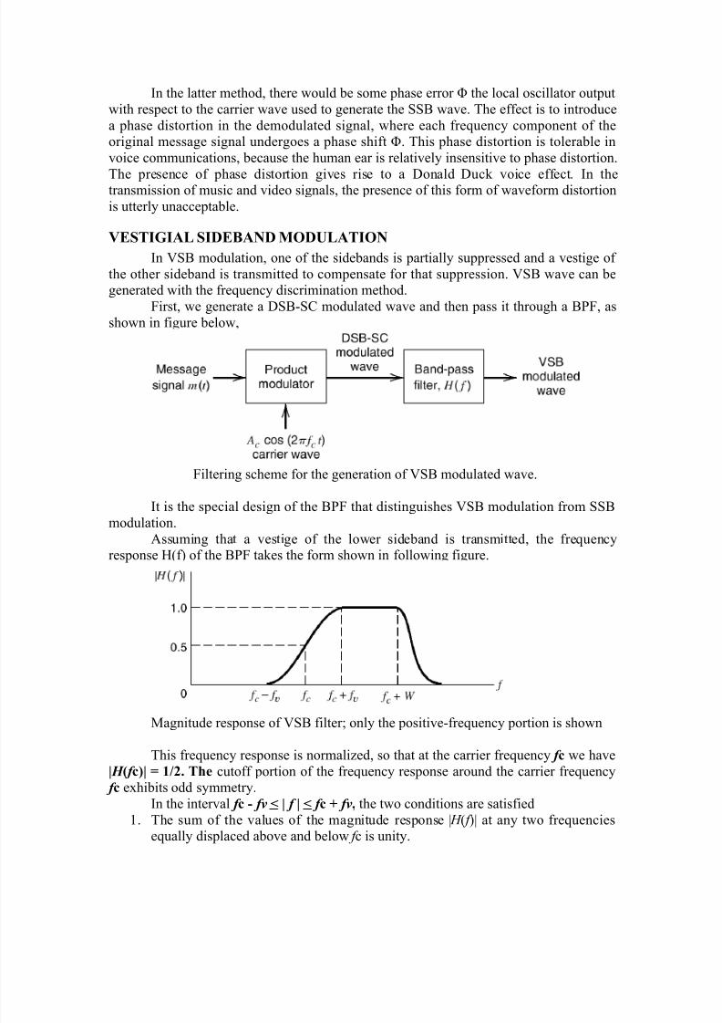
VESTIGIAL SIDEBAND MODULATIONIn VSB modulation, one of the sidebands is partially suppressed and a vestige of
the other sideband is transmitted to compensate for that suppression. VSB wave can begenerated with the frequency discrimination method.
First, we generate a DSB-SC modulated wave and then pass it through a BPF, as
shown in figure below,
Filtering scheme for the generation of VSB modulated wave.
It is the special design of the BPF that distinguishes VSB modulation from SSB
modulation.
Assuming that a vestige of the lower sideband is transmitted, the frequencyresponse H(f) of the BPF takes the form shown in following figure.
Magnitude response of VSB filter; only the positive-frequency portion is shown
This frequency response is normalized, so that at the carrier frequency f c we have| H ( f c)| = 1/2. The cutoff portion of the frequency response around the carrier frequency
f c exhibits odd symmetry. In the interval f c - fv < | f | < f c + fv, the two conditions are satisfied
1. The sum of the values of the magnitude response | H ( f )| at any two frequenciesequally displaced above and below f c is unity.
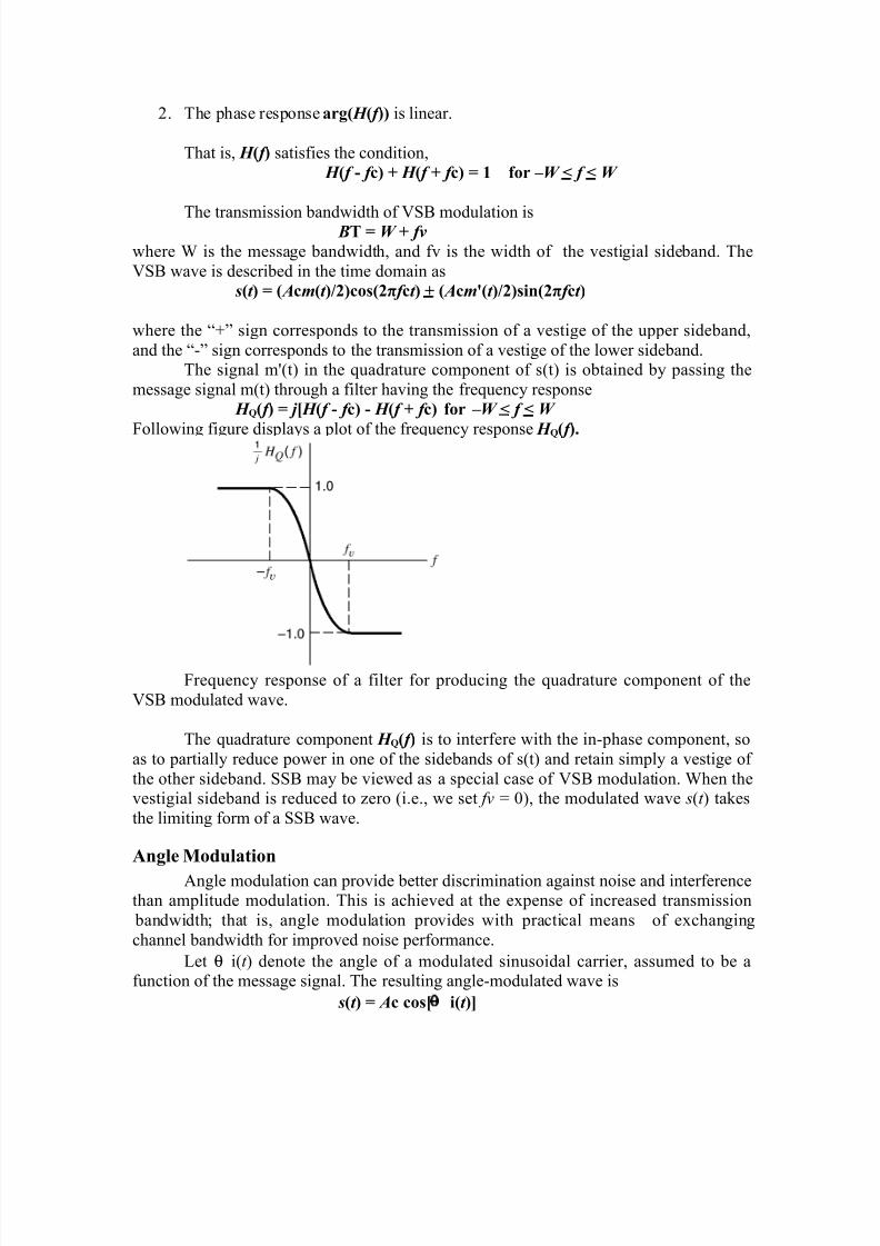
8/8/2019 PSTS 23344
http://slidepdf.com/reader/full/psts-23344 32/67
2. The phase response arg( H ( f )) is linear.
That is, H ( f ) satisfies the condition, H ( f - f c) + H ( f + f c) = 1 for – W < f < W
The transmission bandwidth of VSB modulation is BT = W + fv
where W is the message bandwidth, and fv is the width of the vestigial sideband. The
VSB wave is described in the time domain as
s(t ) = ( Acm(t )/2)cos(2π f ct ) + ( Acm'(t )/2)sin(2π f ct )
where the “+” sign corresponds to the transmission of a vestige of the upper sideband,
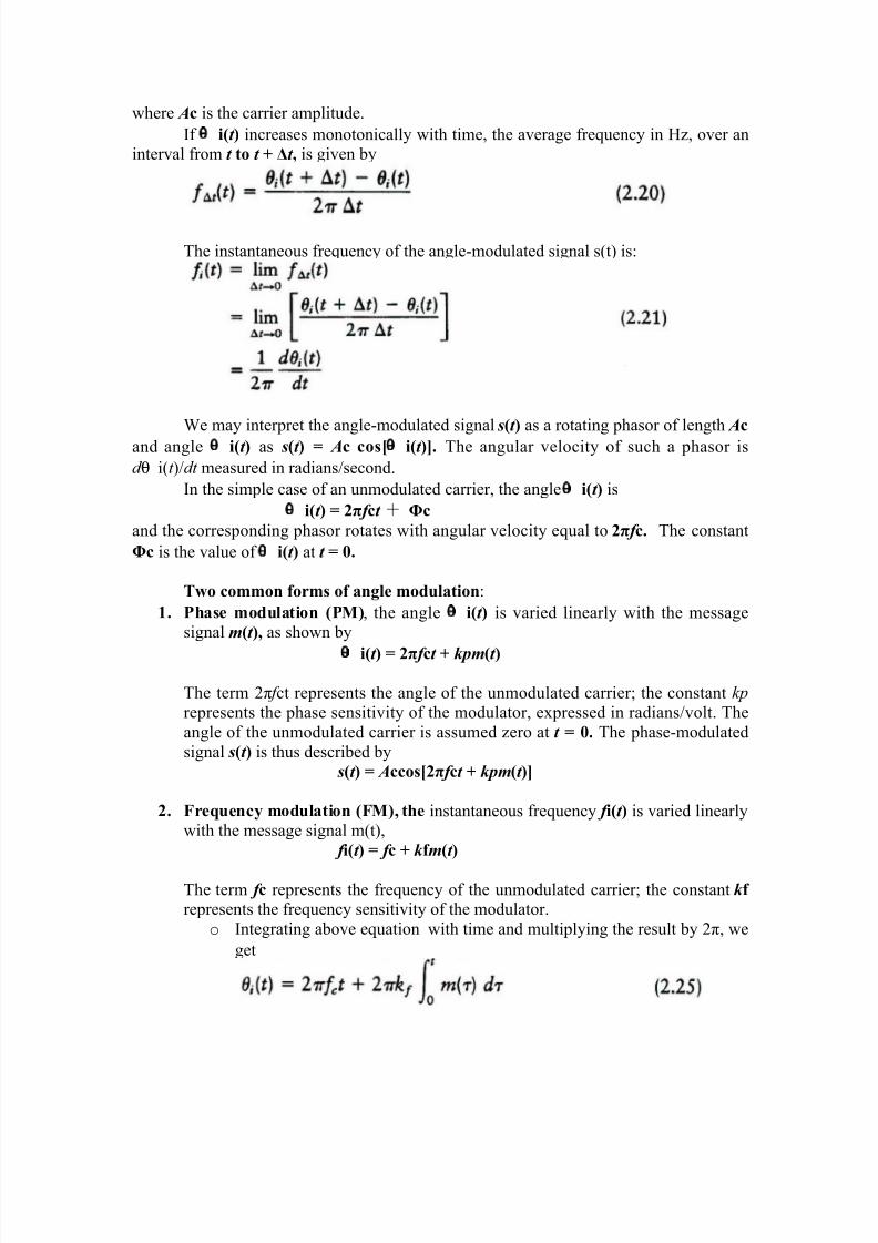
and the “-” sign corresponds to the transmission of a vestige of the lower sideband.The signal m'(t) in the quadrature component of s(t) is obtained by passing the
message signal m(t) through a filter having the frequency response
H Q( f ) = j [ H ( f - f c) - H ( f + f c) for – W < f < W
Following figure displays a plot of the frequency response H Q( f ).
Frequency response of a filter for producing the quadrature component of the
VSB modulated wave.
The quadrature component H Q( f ) is to interfere with the in-phase component, so
as to partially reduce power in one of the sidebands of s(t) and retain simply a vestige of
the other sideband. SSB may be viewed as a special case of VSB modulation. When thevestigial sideband is reduced to zero (i.e., we set fv = 0), the modulated wave s(t ) takes
the limiting form of a SSB wave.
Angle ModulationAngle modulation can provide better discrimination against noise and interference
than amplitude modulation. This is achieved at the expense of increased transmission
bandwidth; that is, angle modulation provides with practical means of exchanging
channel bandwidth for improved noise performance.
Let θ i(t ) denote the angle of a modulated sinusoidal carrier, assumed to be afunction of the message signal. The resulting angle-modulated wave is
s(t ) = Ac cos[θ i(t )]
8/8/2019 PSTS 23344
http://slidepdf.com/reader/full/psts-23344 33/67
where Ac is the carrier amplitude. If θ i(t ) increases monotonically with time, the average frequency in Hz, over an
interval from t to t + Δt , is given by
The instantaneous frequency of the angle-modulated signal s(t) is:
We may interpret the angle-modulated signal s(t ) as a rotating phasor of length Acand angle θ i(t ) as s(t ) = Ac cos[θ i(t )]. The angular velocity of such a phasor is
d θ i(t )/dt measured in radians/second.
In the simple case of an unmodulated carrier, the angle θ i(t ) is
θ i(t ) = 2π f ct + Φcand the corresponding phasor rotates with angular velocity equal to 2π f c. The constant
Φc is the value of θ i(t ) at t = 0.
Two common forms of angle modulation:
1. Phase modulation (PM), the angle θ i(t ) is varied linearly with the messagesignal m(t ), as shown by
θ i(t ) = 2π f ct + kpm(t )
The term 2π f ct represents the angle of the unmodulated carrier; the constant kp
represents the phase sensitivity of the modulator, expressed in radians/volt. The
angle of the unmodulated carrier is assumed zero at t = 0. The phase-modulated
signal s(t ) is thus described by
s(t ) = Accos[2π f ct + kpm(t )]
2. Frequency modulation (FM), the instantaneous frequency f i(t ) is varied linearlywith the message signal m(t),
f i(t ) = f c + k f m(t )
The term f c represents the frequency of the unmodulated carrier; the constant k f represents the frequency sensitivity of the modulator.
o Integrating above equation with time and multiplying the result by 2π, we
get
8/8/2019 PSTS 23344
http://slidepdf.com/reader/full/psts-23344 34/67
where the angle of the unmodulated carrier wave is assumed zero at t = 0.
o The frequency-modulated signal s(t ) is therefore described by
o Allowing the angle θ i(t ) to become dependent on the message signal m(t )
as in θ i(t ) = 2π f ct + kpm(t ) or on its integral as causes the zero crossingsof a PM signal or FM signal no longer have a perfect regularity in their
spacing.
The envelope of a PM or FM signal is constant, whereas the envelope of an AM
signal is dependent on the message signal.
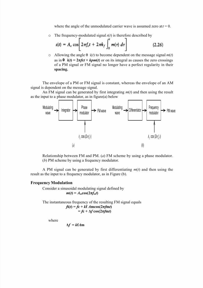
An FM signal can be generated by first integrating m(t ) and then using the resultas the input to a phase modulator, as in figure(a) below
Relationship between FM and PM. (a) FM scheme by using a phase modulator.
(b) PM scheme by using a frequency modulator.
A PM signal can be generated by first differentiating m(t ) and then using theresult as the input to a frequency modulator, as in Figure (b).
Frequency ModulationConsider a sinusoidal modulating signal defined by
m(t ) = Amcos(2π f mt )
The instantaneous frequency of the resulting FM signal equals f i(t ) = f c + k f Amcos(2π f mt )
= f c + Δ f cos(2π f mt )
whereΔ f = k f Am
8/8/2019 PSTS 23344
http://slidepdf.com/reader/full/psts-23344 35/67
The frequency deviation Δ f represents the maximum departure of the
instantaneous frequency of the FM signal from the carrier frequency f c.
• For an FM signal, the frequency deviation Δf is proportional to the amplitude of
the modulating signal and is independent of the modulation frequency.
• The angle θi(t ) of the FM signal is obtained as
• The ratio of the frequency deviation Δf to the modulation frequency fm, iscommonly called the modulation index of the FM signal:
β = Δ f / f m (2.31)and
θ i(t ) = 2π f ct + β sin(2π f mt ) (2.32)
From above equation the parameter β represents the phase deviation of the FM
signal, the maximum departure of the angle θ i(t ) from the angle 2π f ct of theunmodulated carrier; hence, β is measured in radians.
The FM signal itself is given by
s(t ) = Accos[2pπ f ct + bsin(2pπ f mt )]
Depending on the modulation index b, we may distinguish two
cases of FM:
• Narrowband FM, for which b is small compared to one radian.
• Wideband FM, for which b is large compared to one radian.
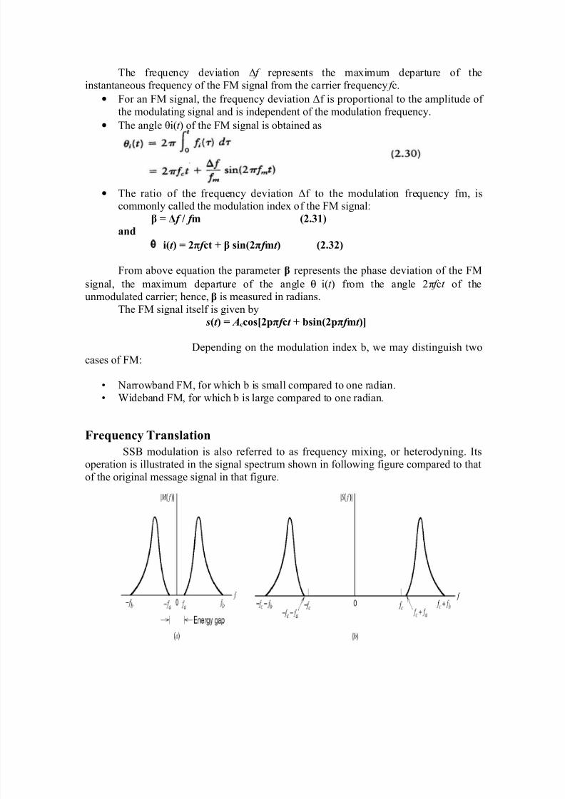
Frequency TranslationSSB modulation is also referred to as frequency mixing, or heterodyning. Its
operation is illustrated in the signal spectrum shown in following figure compared to that
of the original message signal in that figure.
8/8/2019 PSTS 23344
http://slidepdf.com/reader/full/psts-23344 36/67
(a) Spectrum of a message signal m(t) with an energy gap of width 2fa centered on the
origin.(b) Spectrum of corresponding SSB signal containing the upper sideband.
A message spectrum from fa to fb for positive frequencies in Figure(a) shifted
upward by an amount fc and the message spectrum for negative frequencies is translated
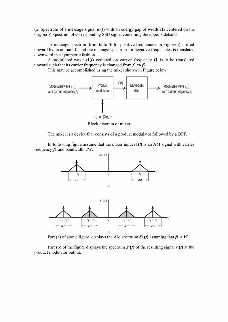
downward in a symmetric fashion.A modulated wave s1(t ) centered on carrier frequency f 1 is to be translated
upward such that its carrier frequency is changed from f 1 to f 2.This may be accomplished using the mixer shown in Figure below,
Block diagram of mixer
The mixer is a device that consists of a product modulator followed by a BPF.
In following figure assume that the mixer input s1(t ) is an AM signal with carrier
frequency f 1 and bandwidth 2W.
Part (a) of above figure displays the AM spectrum S 1( f ) assuming that f 1 > W .
Part (b) of the figure displays the spectrum S '( f ) of the resulting signal s'(t ) at the
product modulator output.

8/8/2019 PSTS 23344
http://slidepdf.com/reader/full/psts-23344 37/67
The signal s'(t ) may be viewed as the sum of two modulated components: one
component represented by the shaded spectrum in Figure (b), and the other represented
by the unshaded spectrum in this figure.Depending on the carrier frequency f 1 is translated upward or downward, we may
identify two different situations:
• Up Conversion: In this case the translated carrier frequency f 2 is greater than theincoming carrier frequency f 1, and the local oscillator frequency f L is defined by
f 2 = f 1 + f Lor
f L = f 2 - f 1
The unshaded spectrum in Figure (b) defines the wanted signal s2(t ) and the
shaded spectrum defines the image signal associated with s2(t ).
• Down Conversion: In this case the translated carrier frequency f2 is smaller than
the incoming carrier frequency f1, and the required oscillator frequency fL is
f2 = f1 – fLor
fL = f1 - f2
The shaded spectrum in Figure (b) defines the wanted modulated signal s2(t), and
the unshaded spectrum defines the associated image signal.
The BPF in the mixer of is to pass the wanted modulated signal s2(t) and toeliminate the associated image signal. This objective is to align the midband frequency of
the filter with f2 and to assign it a bandwidth equal to that of the signal s1(t).
8/8/2019 PSTS 23344
http://slidepdf.com/reader/full/psts-23344 38/67
Chapter 5
Transmission Lines
IntroductionIn an electronic system, the delivery of power requires the connection of two
wires between the source and the load. At low frequencies, power is considered to be
delivered to the load through the wire.
In the microwave frequency region, power is considered to be in electric andmagnetic fields that are guided from lace to place by some physical structure. Any
physical structure that will guide an electromagnetic wave place to place is called aTransmission Line.
Types of Transmission Lines1. Two wire line
2. Coaxial cable
3. Waveguide
Rectangular
Circular
4. Planar Transmission Lines
Strip line
Microstrip line
Slot line
Fin line
Coplanar Waveguide
Coplanar slot line
Analysis of differences between Low and High Frequency• At low frequencies, the circuit elements are lumped since voltage and current waves
affect the entire circuit at the same time.
• At microwave frequencies, such treatment of circuit elements is not possible since
voltage and current waves do not affect the entire circuit at the same time.
• The circuit must be broken down into unit sections within which the circuit elements
are considered to be lumped.
• This is because the dimensions of the circuit are comparable to the wavelength of the
waves according to the formula:λ = c/f
where,
8/8/2019 PSTS 23344
http://slidepdf.com/reader/full/psts-23344 39/67
c = velocity of light
f = frequency of voltage/current
Transmission Line Concepts• The transmission line is divided into small units where the circuit elements can be
lumped.
• Assuming the resistance of the lines is zero, and then the transmission line can be
modeled as an LC ladder network with inductors in the series arms and the
capacitors in the shunt arms.
• The value of inductance and capacitance of each part determines the velocity of
propagation of energy down the line.
• Time taken for a wave to travel one unit length is equal toT(s) = (LC)0.5
• Velocity of the wave is equal tov (m/s) = 1/T
• Impedance at any point is equal to
Z = V (at any point)/I (at any point)Z = (L/C)0.5
• Line terminated in its characteristic impedance:If the end of the transmission line is terminated in a resistor equal in value to the
characteristic impedance of the line as calculated by the formula Z=(L/C) 0.5 , thenthe voltage and current are compatible and no reflections occur.
• Line terminated in a short :When the end of the transmission line is terminated in a short (RL = 0), the
voltage at the short must be equal to the product of the current and the resistance.
• Line terminated in an open:When the line is terminated in an open, the resistance between the open ends of
the line must be infinite. Thus the current at the open end is zero.
Reflection from Resistive loadsWhen the resistive load termination is not equal to the characteristic impedance,
part of the power is reflected back and the remainder is absorbed by the load. The amount
of voltage reflected back is called voltage reflection coefficient.
Γ = Vr/Viwhere Vr = reflected voltage
Vi = incident voltage
The reflection coefficient is also given byΓ = (ZL - ZO)/(ZL + ZO)
8/8/2019 PSTS 23344
http://slidepdf.com/reader/full/psts-23344 40/67
Standing WavesA standing wave is formed by the addition of incident and reflected waves and
has nodal points that remain stationary with time.
• Voltage Standing Wave Ratio:
VSWR = Vmax/Vmin
Voltage standing wave ratio expressed in decibels is called the Standing Wave Ratio:
SWR (dB) = 20log10VSWR • The maximum impedance of the line is given by:
Zmax = Vmax/Imin• The minimum impedance of the line is given by:
Zmin = Vmin/Imaxor alternatively:
Zmin = Zo/VSWR • Relationship between VSWR and Reflection Coefficient:
VSWR = (1 + |Γ|)/(1 - |Γ|)
Γ = (VSWR – 1)/(VSWR + 1)
General Input Impedance EquationInput impedance of a transmission line at a distance L from the load impedance
ZL with a characteristic Zo isZinput = Zo [(ZL + j Zo BL)/(Zo + j ZL BL)]
where B is called phase constant or wavelength constant and is defined by theequation
B = 2π/λ
Half and Quarter wave transmission linesThe relationship of the input impedance at the input of the half-wave transmission
line with its terminating impedance is got by letting L = λ/2 in the impedance equation.Zinput = ZL Ω
The relationship of the input impedance at the input of the quarter-wave
transmission line with its terminating impedance is got by letting L = λ/4 in theimpedance equation.
Zinput = (Zinput Zoutput)0.5 Ω
Effect of Lossy line on voltage and current waves• The effect of resistance in a transmission line is to continuously reduce the
amplitude of both incident and reflected voltage and current waves.
• Skin Effect: As frequency increases, depth of penetration into adjacent
conductive surfaces decreases for boundary currents associated with
electromagnetic waves. This results in the confinement of the voltage and current
waves at the boundary of the transmission line, thus making the transmissionmore lossy.

8/8/2019 PSTS 23344
http://slidepdf.com/reader/full/psts-23344 41/67
• The skin depth is given by:Skin depth (m) = 1/ (πµγf) 0.5
where f = frequency, Hz
µ = permeability, H/m
γ = conductivity, S/m
Smith chartFor complex transmission line problems, the use of the formulae becomes
increasingly difficult and inconvenient. An indispensable graphical method of solution is
the use of Smith Chart.
Components of a Smith Chart• Horizontal line: The horizontal line running through the center of the Smith chart
represents either the resistive or the conductive component. Zero resistance or
conductance is located on the left end and infinite resistance or conductance is
located on the right end of the line.
• Circles of constant resistance and conductance: Circles of constant resistanceare drawn on the Smith chart tangent to the right-hand side of the chart and itsintersection with the centerline. These circles of constant resistance are used to
locate complex impedances and to assist in obtaining solutions to problems
involving the Smith chart.

8/8/2019 PSTS 23344
http://slidepdf.com/reader/full/psts-23344 42/67
• Lines of constant reactance: Lines of constant reactance are shown on the Smith
chart with curves that start from a given reactance value on the outer circle andend at the right-hand side of the center line.
Solutions to Microwave problems using Smith chartThe types of problems for which Smith charts are used include the following:
1. Plotting a complex impedance on a Smith chart
2. Finding VSWR for a given load3. Finding the admittance for a given impedance
4. Finding the input impedance of a transmission line terminated in a short or
open.5. Finding the input impedance at any distance from a load ZL.
6. Locating the first maximum and minimum from any load
7. Matching a transmission line to a load with a single series stub.8. Matching a transmission line with a single parallel stub
9. Matching a transmission line to a load with two parallel stubs.
• Plotting a Complex Impedance on a Smith Chart
o To locate a complex impedance, Z = R+-jX or admittance Y = G +- jB on
a Smith chart, normalize the real and imaginary part of the complex
impedance. Locating the value of the normalized real term on the
horizontal line scale locates the resistance circle. Locating the normalizedvalue of the imaginary term on the outer circle locates the curve of
constant reactance. The intersection of the circle and the curve locates the
complex impedance on the Smith chart.
• Finding the VSWR for a given load
o Normalize the load and plot its location on the Smith chart.o Draw a circle with a radius equal to the distance between the 1.0 point and
the location of the normalized load and the center of the Smith chart as the
center.
o The intersection of the right-hand side of the circle with the horizontal
resistance line locates the value of the VSWR.
• Finding the Input Impedance at any Distance from the Load
o The load impedance is first normalized and is located on the Smith chart.
o The VSWR circle is drawn for the load.
o A line is drawn from the 1.0 point through the load to the outer
wavelength scale.
o To locate the input impedance on a Smith chart of the transmission line at
any given distance from the load, advance in clockwise direction from the
located point, a distance in wavelength equal to the distance to the newlocation on the transmission line.
8/8/2019 PSTS 23344
http://slidepdf.com/reader/full/psts-23344 43/67
8/8/2019 PSTS 23344
http://slidepdf.com/reader/full/psts-23344 44/67
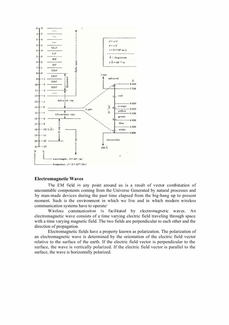
Electromagnetic WavesThe EM field in any point around us is a result of vector combination of
uncountable components coming from the Universe Generated by natural processes and
by man-made devices during the past time elapsed from the big-bang up to presentmoment. Such is the environment in which we live and in which modern wireless
communication systems have to operate/
Wireless communication is facilitated by electromagnetic waves. Anelectromagnetic wave consists of a time varying electric field traveling through space
with a time varying magnetic field. The two fields are perpendicular to each other and the
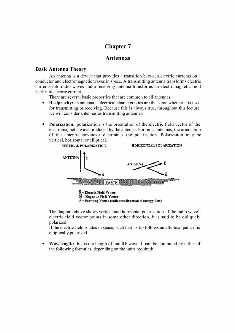
direction of propagation.Electromagnetic fields have a property known as polarization. The polarization of
an electromagnetic wave is determined by the orientation of the electric field vector
relative to the surface of the earth. If the electric field vector is perpendicular to the
surface, the wave is vertically polarized. If the electric field vector is parallel to thesurface, the wave is horizontally polarized.
8/8/2019 PSTS 23344
http://slidepdf.com/reader/full/psts-23344 45/67
Since electromagnetic waves travel through space, space can be thought of as a
kind of transmission line without any conductors, and like other transmission lines it has
characteristic impedance. For free space the characteristic impedance is 377 ohms.The electromagnetic waves that we wish to receive are referred to as signals. The
signals that we don’t want are noise. Interference to the desired signal caused by other
sources of RF waves, man-made or natural is known as RFI (Radio FrequencyInterference). As the number of wireless devices increases, mitigating RFI can become a
full-time job (and headache).
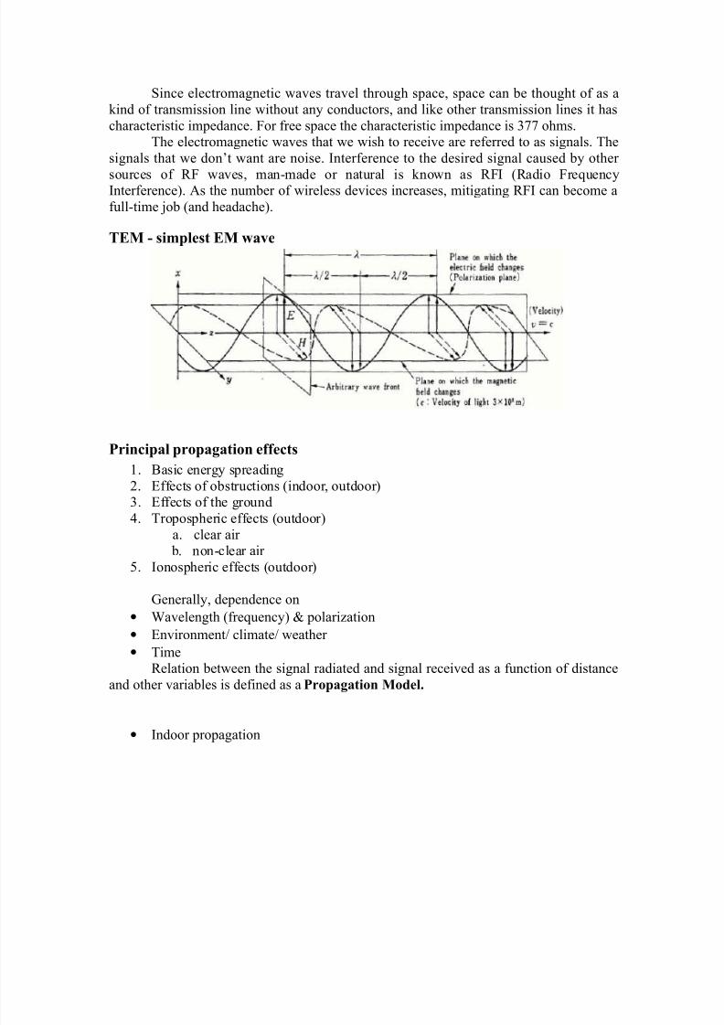
TEM - simplest EM wave
Principal propagation effects1. Basic energy spreading
2. Effects of obstructions (indoor, outdoor)3. Effects of the ground
4. Tropospheric effects (outdoor)
a. clear air b. non-clear air
5. Ionospheric effects (outdoor)
Generally, dependence on
• Wavelength (frequency) & polarization
• Environment/ climate/ weather
• TimeRelation between the signal radiated and signal received as a function of distance
and other variables is defined as a Propagation Model.
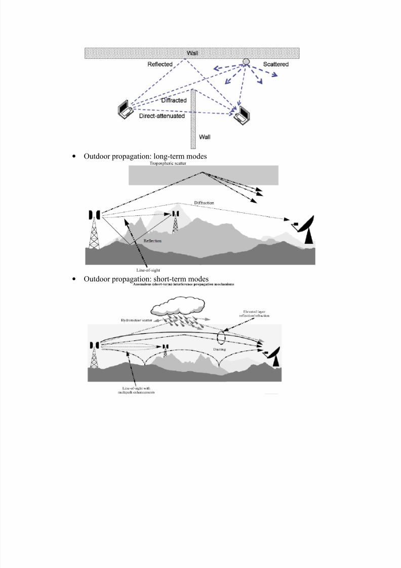
• Indoor propagation
8/8/2019 PSTS 23344
http://slidepdf.com/reader/full/psts-23344 46/67
• Outdoor propagation: long-term modes
• Outdoor propagation: short-term modes
8/8/2019 PSTS 23344
http://slidepdf.com/reader/full/psts-23344 47/67
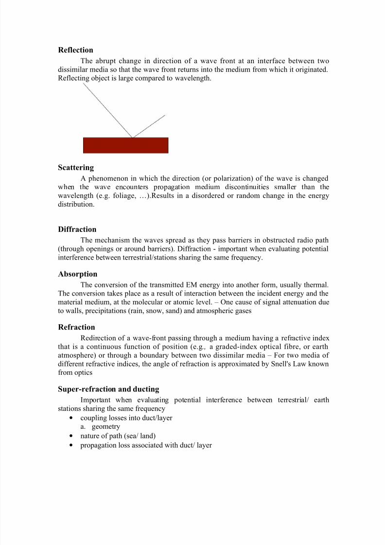
ReflectionThe abrupt change in direction of a wave front at an interface between two
dissimilar media so that the wave front returns into the medium from which it originated.Reflecting object is large compared to wavelength.
ScatteringA phenomenon in which the direction (or polarization) of the wave is changed
when the wave encounters propagation medium discontinuities smaller than the
wavelength (e.g. foliage, …).Results in a disordered or random change in the energy
distribution.
DiffractionThe mechanism the waves spread as they pass barriers in obstructed radio path
(through openings or around barriers). Diffraction - important when evaluating potential
interference between terrestrial/stations sharing the same frequency.
Absorption
The conversion of the transmitted EM energy into another form, usually thermal.The conversion takes place as a result of interaction between the incident energy and the
material medium, at the molecular or atomic level. – One cause of signal attenuation due
to walls, precipitations (rain, snow, sand) and atmospheric gases
RefractionRedirection of a wave-front passing through a medium having a refractive index
that is a continuous function of position (e.g., a graded-index optical fibre, or earth
atmosphere) or through a boundary between two dissimilar media – For two media of
different refractive indices, the angle of refraction is approximated by Snell's Law knownfrom optics
Super-refraction and ductingImportant when evaluating potential interference between terrestrial/ earth
stations sharing the same frequency
• coupling losses into duct/layer a. geometry
• nature of path (sea/ land)
• propagation loss associated with duct/ layer
8/8/2019 PSTS 23344
http://slidepdf.com/reader/full/psts-23344 48/67
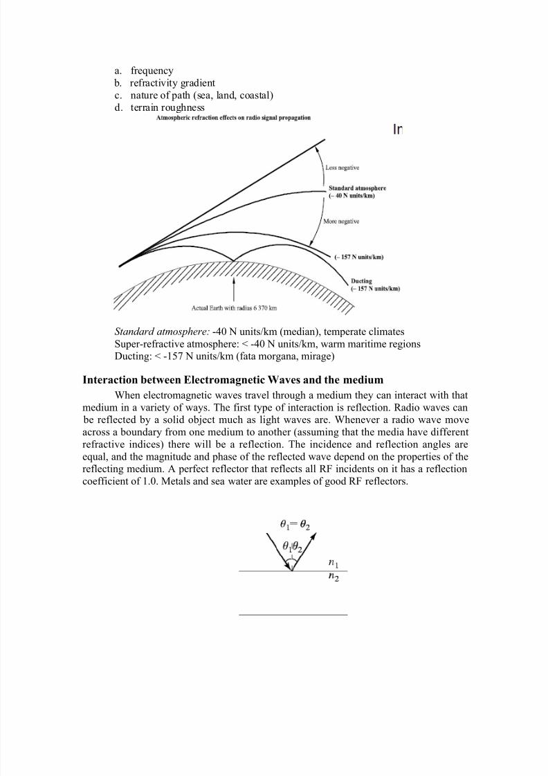
a. frequency
b. refractivity gradient
c. nature of path (sea, land, coastal)d. terrain roughness
Standard atmosphere: -40 N units/km (median), temperate climates
Super-refractive atmosphere: < -40 N units/km, warm maritime regionsDucting: < -157 N units/km (fata morgana, mirage)
Interaction between Electromagnetic Waves and the mediumWhen electromagnetic waves travel through a medium they can interact with that
medium in a variety of ways. The first type of interaction is reflection. Radio waves can be reflected by a solid object much as light waves are. Whenever a radio wave move
across a boundary from one medium to another (assuming that the media have different
refractive indices) there will be a reflection. The incidence and reflection angles are
equal, and the magnitude and phase of the reflected wave depend on the properties of thereflecting medium. A perfect reflector that reflects all RF incidents on it has a reflection
coefficient of 1.0. Metals and sea water are examples of good RF reflectors.

8/8/2019 PSTS 23344
http://slidepdf.com/reader/full/psts-23344 49/67
8/8/2019 PSTS 23344
http://slidepdf.com/reader/full/psts-23344 50/67
Ground Wave PropagationGround Waves are radio waves that follow the curvature of the earth. Ground
waves are always vertically polarized, because a horizontally polarized ground wavewould be shorted out by the conductivity of the ground. Because ground waves are
actually in contact with the ground, they are greatly affected by the ground’s properties.
Because ground is not a perfect electrical conductor, ground waves are attenuated as theyfollow the earth’s surface. This effect is more pronounced at higher frequencies, limiting
the usefulness of ground wave propagation to frequencies below 2 MHz. Ground waves
will propagate long distances over sea water, due to its high conductivity.Ground waves are used primarily for local AM broadcasting and communications
with submarines. Submarine communications takes place at frequencies well below 10
KHz, which can penetrate sea water (remember the skin effect?) and which are
propagated globally by ground waves.
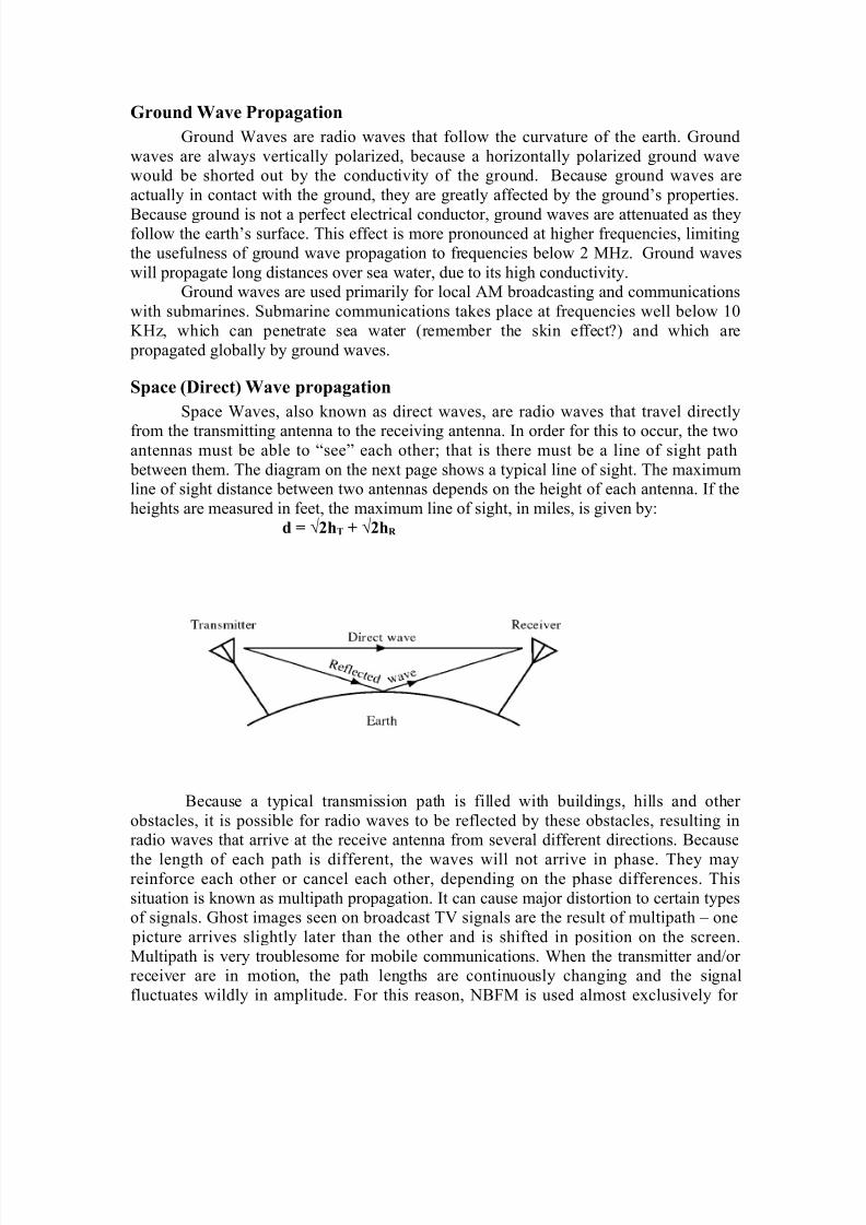
Space (Direct) Wave propagationSpace Waves, also known as direct waves, are radio waves that travel directly
from the transmitting antenna to the receiving antenna. In order for this to occur, the twoantennas must be able to “see” each other; that is there must be a line of sight path
between them. The diagram on the next page shows a typical line of sight. The maximumline of sight distance between two antennas depends on the height of each antenna. If the
heights are measured in feet, the maximum line of sight, in miles, is given by:d = √2hT + √2hR
Because a typical transmission path is filled with buildings, hills and other
obstacles, it is possible for radio waves to be reflected by these obstacles, resulting inradio waves that arrive at the receive antenna from several different directions. Because
the length of each path is different, the waves will not arrive in phase. They mayreinforce each other or cancel each other, depending on the phase differences. This
situation is known as multipath propagation. It can cause major distortion to certain typesof signals. Ghost images seen on broadcast TV signals are the result of multipath – one
picture arrives slightly later than the other and is shifted in position on the screen.
Multipath is very troublesome for mobile communications. When the transmitter and/or receiver are in motion, the path lengths are continuously changing and the signal
fluctuates wildly in amplitude. For this reason, NBFM is used almost exclusively for
8/8/2019 PSTS 23344
http://slidepdf.com/reader/full/psts-23344 51/67
mobile communications. Amplitude variations caused by multipath that make AM
unreadable are eliminated by the limiter stage in an NBFM receiver.
An interesting example of direct communications is satellite communications. If a satellite is placed in an orbit 22,000 miles above the equator, it appears to stand still in
the sky, as viewed from the ground. A high gain antenna can be pointed at the satellite to
transmit signals to it. The satellite is used as a relay station, from which approximately ¼of the earth’s surface is visible. The satellite receives signals from the ground at one
frequency, known as the uplink frequency, translates this frequency to a different
frequency, known as the downlink frequency, and retransmits the signal. Because twofrequencies are used, the reception and transmission can happen simultaneously. A
satellite operating in this way is known as a transponder. The satellite has a tremendous
line of sight from its vantage point in space and many ground stations can communicate
through a single satellite.
Sky Waves
Propagation beyond the line of sight is possible through sky waves. Sky waves areradio waves that propagate into the atmosphere and then are returned to earth at somedistance from the transmitter. We will consider two cases:
• ionospheric refraction
• tropospheric scatter
Ionospheric Refraction
This propagation mode occurs when radio waves travel into the ionosphere, aregion of charged particles 50 – 300 miles above the earth’s surface. The ionosphere is
created when the sun ionizes the upper regions of the earth’s atmosphere. These charged
regions are electrically active. The ionosphere bends and attenuates radio waves atfrequencies below 30 MHz. Above 200 MHz the ionosphere becomes completely
transparent. The ionosphere is responsible for most propagation phenomena observed at
HF, MF, LF and VLF. The ionosphere consists of 4 highly ionized regions
The D layer at a height of 38 – 55 mi
The E layer at a height of 62 – 75 mi
The F1 layer at a height of 125 –150 mi (winter) and 160 – 180 mi (summer)The F2 layer at a height of 150 – 180 mi (winter) and 240 – 260 mi (summer)
The density of ionization is greatest in the F layers and least in the D layer
Though created by solar radiation, the ionosphere does not completely disappear shortlyafter sunset. The D and E layers disappear almost immediately, but the F1 and F2 layers
do not disappear; rather they merge into a single F layer located at a distance of 150 – 250 mi above the earth. Recombination or charged particles is quite slow at that altitude,
so the F layer lasts until dawn.

8/8/2019 PSTS 23344
http://slidepdf.com/reader/full/psts-23344 52/67
The diagram below shows the geometry of ionospheric refraction. The maximum
frequency that can be returned by the ionosphere when the radio waves are vertically
incident on the ionosphere (transmitted straight up) is called the critical frequency.
The critical frequency varies from place to place, and it is possible to view thisvariation by looking at a real-time critical frequency map
The critical frequency varies from 1 to 15 MHz under normal conditions. Most
communications is done using radio waves transmitted at the horizon, to get the
maximum possible distance per hop. The highest frequency that can be returned when thetakeoff angle is zero degrees is called the MUF, maximum usable frequency. The MUF
and critical frequency are related by the following formula:
The MUF can range from 3 to 50 MHz. You can click here to see a near real-time
map of the MUF of the ionosphere.

8/8/2019 PSTS 23344
http://slidepdf.com/reader/full/psts-23344 53/67
The ionosphere also attenuates radio waves. The amount of attenuation is
roughly inversely proportional to the square of the frequency of the wave. Thus
attenuation is a severe problem at lower frequencies, making daytime globalcommunications via sky wave impossible at frequencies much below 5 MHz.
The properties of the ionosphere are variable. There are 3 periodic cycles of
variation:
• Diurnal (daily) cycle
• Seasonal cycle
• Sunspot cycle
The daily cycle is driven by the intensity of the solar radiation ionizing the upper atmosphere. The D and E layers form immediately after sunrise and the F layer splits into
two layers, the F1 and F2. The density of the layers increases until noon and thendecreases slowly throughout the afternoon. After sunset, the D and E layers disappear and
the F1 and F2 merge to form the F layer. Take another look at the real-time MUF map
and notice the difference between the MUF numbers in the day and night regions. If youaren't sure which region is the daytime region, it has a small yellow sun icon in its center.
The thick gray lines indicate the location of the terminator - the division between day and
night.Seasonal variation is linked to the tilt of the earth’s axis and the distance between
the earth and sun. The effects are complex, but the result is that ionospheric propagation
improves dramatically during the for the northern hemisphere during their winter, whileseasonal variation in the southern hemisphere is much smaller.
The 11 year sunspot cycle exerts a tremendous effect on the atmosphere. Near the
peak of the cycle (the last peak occurred in December 2001) the sun’s surface is very
active, emitting copious amounts of UV radiation and charged particles, which increasethe density of the ionosphere. This leads to a general increase in MUF’s and attenuation
at lower frequencies. When the sun becomes extremely active, or a major solar flare

8/8/2019 PSTS 23344
http://slidepdf.com/reader/full/psts-23344 54/67
occurs, the ionosphere can become so dense that global ionospheric communications are
disrupted.
The maximum distance that can be covered by a single hop using ionospheric
propagation is about 2500 miles. Greater distances can be covered using multi-hop
propagation, in which radio waves are reflected by the ground back up to the ionosphere.The ionosphere is not uniform and different regions refract RF differently.
Multipath propagation is the result. This leads to rapid variations in the received signal
amplitude known as fading.
8/8/2019 PSTS 23344
http://slidepdf.com/reader/full/psts-23344 55/67
Chapter 7
AntennasBasic Antenna Theory
An antenna is a device that provides a transition between electric currents on a
conductor and electromagnetic waves in space. A transmitting antenna transforms electriccurrents into radio waves and a receiving antenna transforms an electromagnetic field
back into electric current.
There are several basic properties that are common to all antennas:
• Reciprocity: an antenna’s electrical characteristics are the same whether it is used
for transmitting or receiving. Because this is always true, throughout this lecture,
we will consider antennas as transmitting antennas.
• Polarization: polarization is the orientation of the electric field vector of the
electromagnetic wave produced by the antenna. For most antennas, the orientationof the antenna conductor determines the polarization. Polarization may be
vertical, horizontal or elliptical.
The diagram above shows vertical and horizontal polarization. If the radio wave's
electric field vector points in some other direction, it is said to be obliquely
polarized.If the electric field rotates in space, such that its tip follows an elliptical path, it is
elliptically polarized.
• Wavelength: this is the length of one RF wave. It can be computed by either of
the following formulas, depending on the units required:

8/8/2019 PSTS 23344
http://slidepdf.com/reader/full/psts-23344 56/67
λ (in m) = 300/f(in MHz) or λ (in ft) = 984/f(in MHz)
• Gain (directivity): This is a measure of the degree to which an antenna focuses
power in a given direction, relative to the power radiated by a reference antenna
in the same direction. Units of measure are dBi (isotopic antenna reference) or dBd (half-wave dipole reference). The two gain measurements can be converted
using the following formula:
dBi = dBd + 2.1
If the directivity of the transmitting and receiving antennas is known, it is possible
to compute the power received by the receiving antenna using either of the
formulas below:
o When using dB:
Antenna gain should be expressed in dBi, wavelength and distances in m and
powers in dBm or dBW.
o When using gain ratios and powers in W:
Antenna gains should be expressed as a number, distances and wavelengths in m
and powers in W.
• Beamwidth: the angular separation between the half-point (-3dB) points in an
antenna’s radiation pattern. In general, the beamwidth of the main lobe of theradiation pattern decreases as the directivity increases.
• Near field (induction field): electromagnetic field created by an antenna that is
only significant at distances of less than 2D/λ from the antenna, where D is thelongest dimension of the antenna.
• Near field region: A spherical region of radius 2D/λ centered on the antenna.
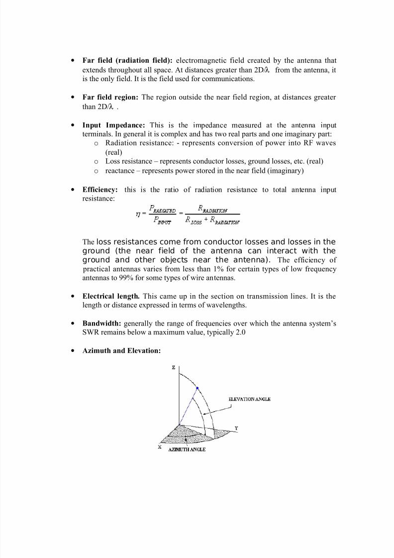
8/8/2019 PSTS 23344
http://slidepdf.com/reader/full/psts-23344 57/67
• Far field (radiation field): electromagnetic field created by the antenna that
extends throughout all space. At distances greater than 2D/λ from the antenna, itis the only field. It is the field used for communications.
• Far field region: The region outside the near field region, at distances greater than 2D/λ .
• Input Impedance: This is the impedance measured at the antenna inputterminals. In general it is complex and has two real parts and one imaginary part:
o Radiation resistance: - represents conversion of power into RF waves
(real)
o Loss resistance – represents conductor losses, ground losses, etc. (real)
o reactance – represents power stored in the near field (imaginary)
• Efficiency: this is the ratio of radiation resistance to total antenna input
resistance:
The loss resistances come from conductor losses and losses in theground (the near field of the antenna can interact with theground and other objects near the antenna). The efficiency of
practical antennas varies from less than 1% for certain types of low frequencyantennas to 99% for some types of wire antennas.
• Electrical length. This came up in the section on transmission lines. It is thelength or distance expressed in terms of wavelengths.
• Bandwidth: generally the range of frequencies over which the antenna system’sSWR remains below a maximum value, typically 2.0
• Azimuth and Elevation:
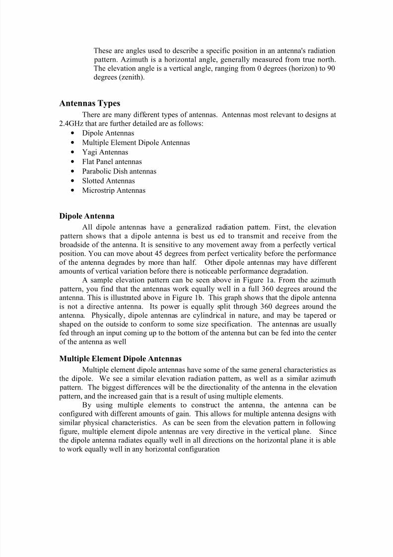
8/8/2019 PSTS 23344
http://slidepdf.com/reader/full/psts-23344 58/67
These are angles used to describe a specific position in an antenna's radiation
pattern. Azimuth is a horizontal angle, generally measured from true north.
The elevation angle is a vertical angle, ranging from 0 degrees (horizon) to 90degrees (zenith).
Antennas TypesThere are many different types of antennas. Antennas most relevant to designs at
2.4GHz that are further detailed are as follows:
• Dipole Antennas
• Multiple Element Dipole Antennas
• Yagi Antennas
• Flat Panel antennas
• Parabolic Dish antennas
• Slotted Antennas
• Microstrip Antennas
Dipole AntennaAll dipole antennas have a generalized radiation pattern. First, the elevation
pattern shows that a dipole antenna is best us ed to transmit and receive from the broadside of the antenna. It is sensitive to any movement away from a perfectly vertical
position. You can move about 45 degrees from perfect verticality before the performance
of the antenna degrades by more than half. Other dipole antennas may have differentamounts of vertical variation before there is noticeable performance degradation.
A sample elevation pattern can be seen above in Figure 1a. From the azimuth
pattern, you find that the antennas work equally well in a full 360 degrees around theantenna. This is illustrated above in Figure 1b. This graph shows that the dipole antenna
is not a directive antenna. Its power is equally split through 360 degrees around the
antenna. Physically, dipole antennas are cylindrical in nature, and may be tapered or
shaped on the outside to conform to some size specification. The antennas are usuallyfed through an input coming up to the bottom of the antenna but can be fed into the center
of the antenna as well
Multiple Element Dipole AntennasMultiple element dipole antennas have some of the same general characteristics as
the dipole. We see a similar elevation radiation pattern, as well as a similar azimuth
pattern. The biggest differences will be the directionality of the antenna in the elevation pattern, and the increased gain that is a result of using multiple elements.By using multiple elements to construct the antenna, the antenna can be
configured with different amounts of gain. This allows for multiple antenna designs with
similar physical characteristics. As can be seen from the elevation pattern in following
figure, multiple element dipole antennas are very directive in the vertical plane. Sincethe dipole antenna radiates equally well in all directions on the horizontal plane it is able
to work equally well in any horizontal configuration
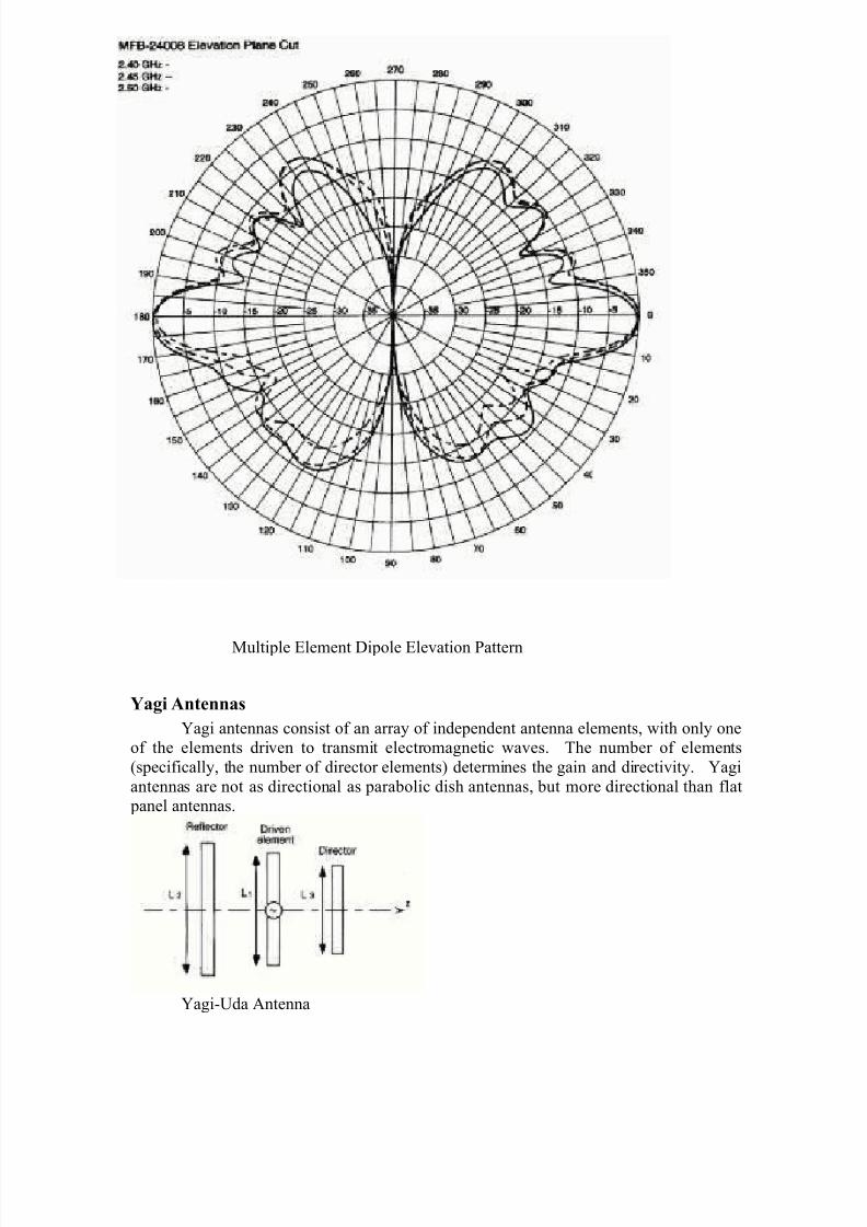
8/8/2019 PSTS 23344
http://slidepdf.com/reader/full/psts-23344 59/67
Multiple Element Dipole Elevation Pattern
Yagi AntennasYagi antennas consist of an array of independent antenna elements, with only one
of the elements driven to transmit electromagnetic waves. The number of elements
(specifically, the number of director elements) determines the gain and directivity. Yagi
antennas are not as directional as parabolic dish antennas, but more directional than flat panel antennas.
Yagi-Uda Antenna
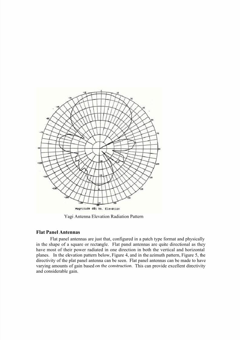
8/8/2019 PSTS 23344
http://slidepdf.com/reader/full/psts-23344 60/67
Yagi Antenna Elevation Radiation Pattern
Flat Panel Antennas
Flat panel antennas are just that, configured in a patch type format and physicallyin the shape of a square or rectangle. Flat panel antennas are quite directional as they
have most of their power radiated in one direction in both the vertical and horizontal planes. In the elevation pattern below, Figure 4, and in the azimuth pattern, Figure 5, the
directivity of the plat panel antenna can be seen. Flat panel antennas can be made to have
varying amounts of gain based on the construction. This can provide excellent directivityand considerable gain.
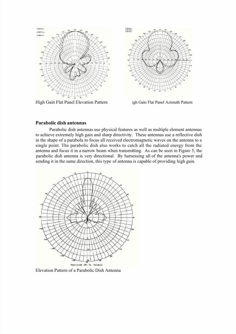
8/8/2019 PSTS 23344
http://slidepdf.com/reader/full/psts-23344 61/67

8/8/2019 PSTS 23344
http://slidepdf.com/reader/full/psts-23344 62/67
Slotted AntennasThe slotted antenna exhibits radiation characteristics that are very similar to those
of the dipole. The elevation and azimuth patterns are similar to those of the dipole, butits physical construction consists only of a narrow slot cut into ground plane. As with
microstrip antennas mentioned below, slotted antennas provide little antenna gain, and do
not exhibit high directionality, as evidenced by their radiation plots and their similarity tothe dipoles. Their most attractive feature is the ease with which they can be constructed
and integrated into an existing design, and their low cost. These factors most often offset
their mediocre performance characteristics.
Microstrip AntennasMicrostrip antennas can be made to emulate many of the different styles of
antennas explained above. Microstrip antennas offer several tradeoffs that need to be
considered. Because they are manufactured with PCB traces on actual PCB boards, they
can be very small and lightweight. This comes at the cost of not being able to handle as
much output power as other antennas, and they are made for very specific frequency
ranges. In many cases, limiting the frequencies that can be received is actually beneficialto the performance of a radio. Due to this characteristic, microstrip antennas are not well
suited for wideband communications systems.
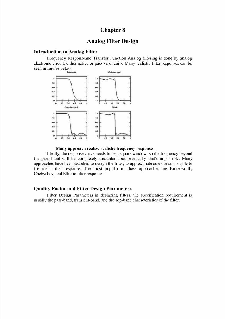
8/8/2019 PSTS 23344
http://slidepdf.com/reader/full/psts-23344 63/67
Chapter 8
Analog Filter Design
Introduction to Analog FilterFrequency Responseand Transfer Function Analog filtering is done by analog
electronic circuit, either active or passive circuits. Many realistic filter responses can beseen in figures below:
Many approach realize realistic frequency responseIdeally, the response curve needs to be a square window, so the frequency beyond
the pass band will be completely discarded, but practically that's impossible. Many
approaches have been searched to design the filter, to approximate as close as possible to
the ideal filter response. The most popular of these approaches are Butterworth,Chebyshev, and Elliptic filter response.
Quality Factor and Filter Design Parameters Filter Design Parameters in designing filters, the specification requirement is
usually the pass-band, transient-band, and the sop-band characteristics of the filter.
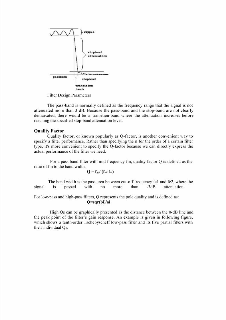
8/8/2019 PSTS 23344
http://slidepdf.com/reader/full/psts-23344 64/67
Filter Design Parameters
The pass-band is normally defined as the frequency range that the signal is not
attenuated more than 3 dB. Because the pass-band and the stop-band are not clearlydemarcated, there would be a transition-band where the attenuation increases before
reaching the specified stop-band attenuation level.
Quality FactorQuality factor, or known popularly as Q-factor, is another convenient way to
specify a filter performance. Rather than specifying the n for the order of a certain filter type, it's more convenient to specify the Q-factor because we can directly express the
actual performance of the filter we need.
For a pass band filter with mid frequency fm, quality factor Q is defined as the
ratio of fm to the band width. Q = f m / (f c2-f c1)
The band width is the pass area between cut-off frequency fc1 and fc2, where the
signal is passed with no more than -3dB attenuation.
For low-pass and high-pass filters, Q represents the pole quality and is defined as:
Q=sqr(bi)/ai
High Qs can be graphically presented as the distance between the 0-dB line andthe peak point of the filter’s gain response. An example is given in following figure,
which shows a tenth-order Tschebyscheff low-pass filter and its five partial filters withtheir individual Qs.
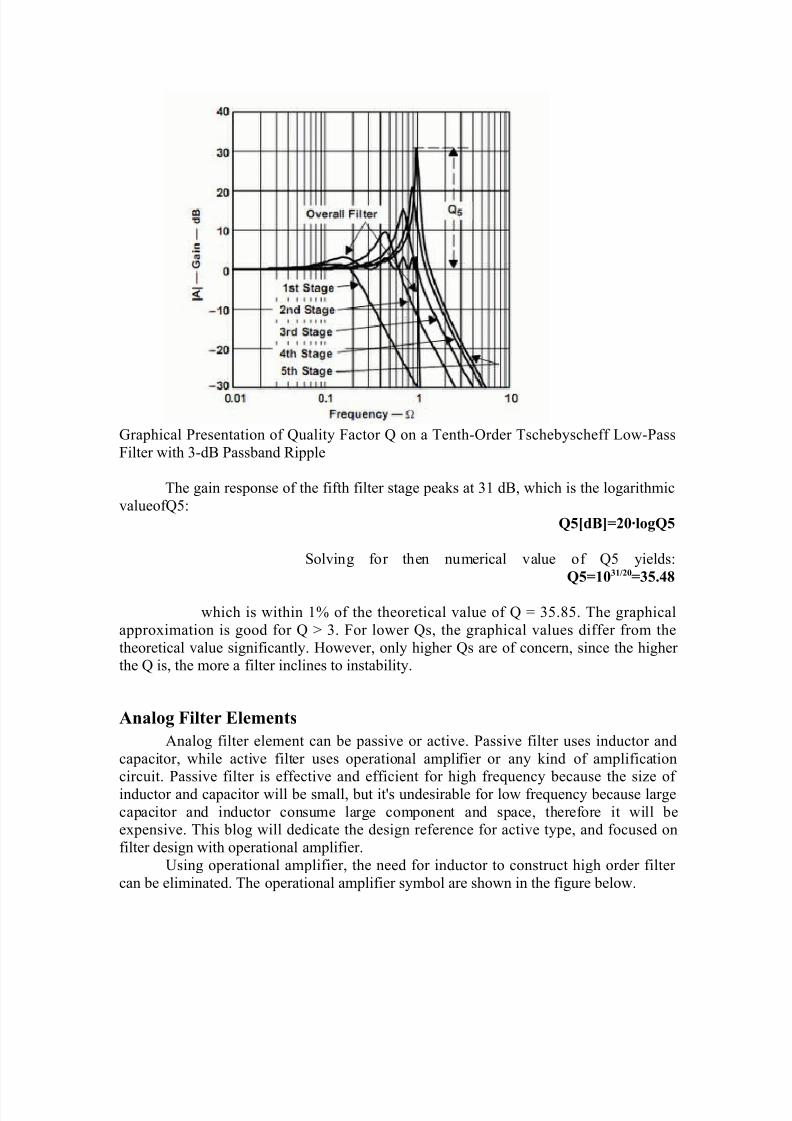
8/8/2019 PSTS 23344
http://slidepdf.com/reader/full/psts-23344 65/67
Graphical Presentation of Quality Factor Q on a Tenth-Order Tschebyscheff Low-Pass
Filter with 3-dB Passband Ripple
The gain response of the fifth filter stage peaks at 31 dB, which is the logarithmic
valueofQ5:
Q5[dB]=20·logQ5
Solving for then numerical value of Q5 yields:
Q5=1031/20=35.48
which is within 1% of the theoretical value of Q = 35.85. The graphical
approximation is good for Q > 3. For lower Qs, the graphical values differ from the
theoretical value significantly. However, only higher Qs are of concern, since the higher the Q is, the more a filter inclines to instability.
Analog Filter ElementsAnalog filter element can be passive or active. Passive filter uses inductor and
capacitor, while active filter uses operational amplifier or any kind of amplificationcircuit. Passive filter is effective and efficient for high frequency because the size of
inductor and capacitor will be small, but it's undesirable for low frequency because large
capacitor and inductor consume large component and space, therefore it will beexpensive. This blog will dedicate the design reference for active type, and focused on
filter design with operational amplifier.
Using operational amplifier, the need for inductor to construct high order filter
can be eliminated. The operational amplifier symbol are shown in the figure below.
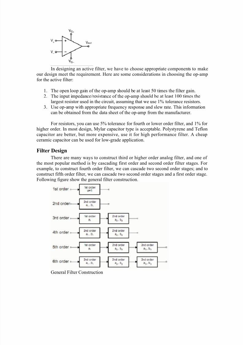
8/8/2019 PSTS 23344
http://slidepdf.com/reader/full/psts-23344 66/67
In designing an active filter, we have to choose appropriate components to makeour design meet the requirement. Here are some considerations in choosing the op-amp
for the active filter:
1. The open loop gain of the op-amp should be at least 50 times the filter gain.
2. The input impedance/resistance of the op-amp should be at least 100 times thelargest resistor used in the circuit, assuming that we use 1% tolerance resistors.
3. Use op-amp with appropriate frequency response and slew rate. This information
can be obtained from the data sheet of the op-amp from the manufacturer.
For resistors, you can use 5% tolerance for fourth or lower order filter, and 1% for higher order. In most design, Mylar capacitor type is acceptable. Polystyrene and Teflon
capacitor are better, but more expensive, use it for high performance filter. A cheap
ceramic capacitor can be used for low-grade application.
Filter DesignThere are many ways to construct third or higher order analog filter, and one of
the most popular method is by cascading first order and second order filter stages. For
example, to construct fourth order filter, we can cascade two second order stages; and to
construct fifth order filter, we can cascade two second order stages and a first order stage.
Following figure show the general filter construction.
General Filter Construction

8/8/2019 PSTS 23344
http://slidepdf.com/reader/full/psts-23344 67/67
The infinite input and zero output approximation of active filter designed with op-
amp make the cascading produce non-interacting stages, therefore the transfer function of
each stage remain unchanged, giving the total cascaded output response equivalent to themultiplication product of their individual transfer functions.
The first order and the second order stages is easy to design, and using design
reference presented here will be easy to construct many types of high filters (high-pass,low-pass, band-pass) with many approach (Butterworth, Chebyshev, Elliptic).
Recommended


![TAP TAP Basics (Preparing for Success in a TAP School) [PSTS]](https://img.dokumen.tips/doc/110x75/56649eb25503460f94bb9499/tap-tap-basics-preparing-for-success-in-a-tap-school-psts.jpg)