Price Caps, Oligopoly, and Entry ∗
Stanley S. Reynolds† David Rietzke‡
July 10, 2013
Abstract
We examine the impact of price caps in oligopoly markets with endogenous
entry. In the case of deterministic demand and constant marginal cost, reducing a
price cap yields increased total output, consumer welfare, and total welfare. This
result falls in line with classic results on price caps in monopoly markets, and with
recent results for oligopoly markets with a fixed number of firms. However, when
demand is deterministic and marginal cost is increasing, a welfare improving price
cap may not exist. We also show that a welfare-improving cap need not exist
in the case where demand is stochastic. The fact that a welfare-improving cap
cannot be guaranteed in these two cases points to a sharp difference in results
between an endogenous entry model and oligopoly models with a fixed number
of firms. Finally, we provide sufficient conditions that ensure the existence of a
welfare-improving cap in the case of stochastic demand.
Keywords: Price Caps; Market Entry; Oligopoly; Demand Uncertainty
∗We thank Rabah Amir, Veronika Grimm, Andras Niedermayer and Gregor Zoettl for helpfulcomments and suggestions.†University of Arizona, Department of Economics, P.O. Box 210108, Tucson, AZ 85721,
[email protected]‡(Corresponding Author) University of Arizona, Department of Economics, P.O. Box 210108, Tuc-
son, AZ 85721, [email protected]

1 Introduction
Price ceilings or caps are relevant in many areas including: wholesale electricity mar-
kets, interest on loans and credit, telecommunications services, taxi services, and hous-
ing in densely populated areas. For instance, regulators have imposed price caps in
a number of U.S. regional wholesale electricity markets, including ERCOT (Texas),
New England, and PJM. A key goal for price caps in wholesale electricity markets is
to limit the exercise of market power. The principle that a price cap can limit market
power is well understood in the case of a monopolist with constant marginal cost in
a perfect-information environment. A price cap increases marginal revenue in those
situations where it is binding and incentivizes the monopolist to increase output. Total
output, consumer surplus, and total welfare are decreasing in the price cap.
Recent papers by Earle, Schmedders and Tatur [2007] and Grimm and Zottl [2010]
examine the effectiveness of price caps in Cournot oligopolies with constant marginal
cost. Earle et al. [2007] show that while the classic monopoly results for price caps carry
over to oligopoly when demand is certain, these results do not hold under demand un-
certainty. In particular, they demonstrate that when firms must make output decisions
prior to the realization of demand, total output, welfare, and consumer surplus may
be locally increasing in the price cap. This result raises into question the effectiveness
of price caps as a welfare-enhancing policy tool. On the other hand, Grimm and Zottl
[2010] demonstrate that, within the framework of Cournot oligopoly with uncertain
demand analyzed by Earle, et al., there exists an interval of prices such that any price
cap in this interval increases both total market output and welfare compared to the
no-cap case. Thus, while the standard comparative statics results of price caps do not
hold with uncertain demand, there always exists a welfare-improving price cap.
Importantly, prior analyses of oligopoly markets with price caps assume that the
number of firms is held fixed. In this paper we explore an additional margin upon
which a price cap may operate; firm entry decisions. We modify the analyses of Earle
et al. [2007] and Grimm and Zottl [2010] by introducing an initial market entry period
prior to a second period of product market competition. Market entry requires a firm
to incur a sunk cost prior to period two product market competition. The inclusion
of a sunk entry cost introduces economies of scale into the analysis. This would seem
to be a natural formulation, since an oligopolistic market structure in a homogeneous
product market may well be present because of economies of scale.1
1Cottle and Wallace [1983] consider a possible reduction in the number of firms in their analysis
1
Our model of endogenous entry builds on results and insights from Mankiw and
Whinston [1986] and Amir and Lambson [2000]. Mankiw and Whinston show that
when total output is increasing in the number of firms but per-firm output is decreasing
in the number of firms (the term for the latter is the business-stealing effect), the
socially optimal number of firms will be less than the free-entry number of firms when
the number of firms, n, is continous. For discrete n the free entry number of firms
may be less than the socially optimal number of firms, but never by more than one.
Intuitively, when a firm chooses to enter, it does not take into account decreases in
per-firm output and profit of the other active firms. Thus, the social gain from entry
may be less than the private gain to the firm. Amir and Lambson [2000] provide a
taxonomy of the effects of entry on output in Cournot markets. In particular, they
provide a very general condition under which equilibrium total output is increasing in
the number of firms. Our analysis relies heavily on their approach and results. We
demonstrate that Amir and Lambson’s condition under which total output is increasing
in the number of firms is also a sufficient condition for total output to be increasing in
the number of firms when their is a price cap.
Our objective is to analyze the impact of price caps in oligopoly markets in which
entry decisions are endogenous. Given the prominent use of price ceilings or caps as a
regulatory tool in settings with multiple suppliers, we believe that an analysis that fails
to consider their impact on market entry decisions may be missing a potentially vital
component. We show that when entry is endogenous, demand is deterministic, and
marginal cost is constant, the standard comparative statics results continue to hold.
In this case, a price cap may result in fewer firms, but the incentive provided by the
cap to increase output overwhelms the incentive to withold output due to a decrease in
competition. It follows that, regardless of the number of firms that enter the market,
output will always increase as the cap is lowered. Welfare gains are realized on two
fronts. First, the cap increases total output. Second, the cap may deter entry, and in
doing so, reduce the total cost associated with entry.
We also consider the case of increasing marginal costs of production. Given our
assumption of a sunk cost of entry, this case implies U-shaped average cost curves for
firms. We show that when demand is deterministic and marginal cost is increasing,
the standard comparative statics results do not hold when entry is endogenous. In
contrast to results for a fixed number of firms, it may be the case that any price cap
of a price ceiling in a perfectly competitive market subject to demand uncertainty. Our interest is inthe impact of price caps in oligopoly markets in which entry is endogenous.
2

reduces total output and welfare (i.e., there does not exist a welfare improving cap).
Moreover, we demonstrate that if marginal cost is increasing sufficiently fast, it may
be the case that the standard comparative statics results are reversed; that is, welfare
and output are increasing in the price cap.
Finally, we demonstrate that a welfare-improving price cap may not exist when
demand is uncertain and entry is endogenous (for constant marginal cost). Thus,
the results of Grimm and Zottl do not generalize to the case of endogenous entry.
We provide sufficient conditions for existence of a welfare-improving price cap. These
conditions restrict the curvature of inverse demand, which in turn influences the extent
of the business-stealing effect when an additional firm enters the market. We also
consider a version of the model with disposal; firms do not have to sell the entire
quantity they produced, but instead may choose the amount to sell after demand
uncertainty has been resolved. We show that the sufficient condition for existence of a
welfare improving price cap for the no-disposal model carries over to the model with
disposal.
2 The Model
We assume there is an arbitrarily large number, N ∈ N, of symmetric potential market
entrants. We formulate a two period game. The N potential entrants are ordered in
a queue and make sequential entry decisions in period one. Each firm’s entry decision
is assumed to be observed by the other firms. We assume that there is a cost of entry
K > 0 which is sunk if a firm enters. If a firm does not enter it receives a payoff of
zero.
Each of the n market entrants produces a homogeneous good in period two. Each
firm has a convex production cost function C : R+ → R+. Output decisions are made
simultaneously. The inverse demand function is given by P (Q, θ) which depends on
total output, Q, and a random variable, θ. θ is continuously distributed according
to CDF F with corresponding density f . The support of θ is bounded and given by
Θ ≡ [θ, θ] ⊂ R. Each firm knows the distribution of θ but must make its output
decision prior to its realization. We assume that a regulator may impose a price cap,
denoted p. The following assumption is in effect throughout the paper.
3
Assumption 1.
(a) P is continuous in Q and θ, strictly decreasing in Q for fixed θ, and strictly in-
creasing in θ for fixed Q.
(b) limQ→∞[P (Q, θ)− C ′(Q)] < 0
(c) maxQ∈R+
E[QP (Q, θ)− C(Q)] > K
Assumption (1a) matches the assumptions imposed by Earle et al. [2007]; Grimm and
Zottl [2010] additionally assume differentiability of inverse demand in Q and θ. As-
sumption (1b) insures that a profit-maximizing quantity exists for period two decisions.
Earle et al. [2007] assumed that E[P (0, θ)] > c (they assume that marginal cost is
a constant, c). Their assumption ensured that “production is gainful”; that is, given a
fixed number, n > 0, of market participants, there exist price caps such that equilibrium
market output will be strictly positive. Our assumption (1c) is a “profitable entry”
condition which guarantees that there exist price caps such that at least one firm enters
the market and that equilibrium output will be strictly positive. We let P denote the
set of price caps which induce at least one market entrant. That is
P ≡{p > 0 | max
Q∈R+
E [Qmin{P (Q, θ), p} − C(Q)] ≥ K
}In this paper we are only concerned with price caps p ∈ P. In the analysis that follows,
we restrict attention to subgame-perfect pure strategy equilibria and focus on period
two subgame equilibria that are symmetric with respect to the set of market entrants.
For a given price cap and a fixed number of firms, there may exist multiple pe-
riod two subgame equilibria. As is common in the oligopoly literature we focus on
extremal equilibria - the equilibria with the smallest and largest total output levels -
and comparisons between extremal equilibria. So when there is a change in the price
cap we compare equilibrium outcomes before and after the change, taking into account
the change (if any) in the equilibrium number of firms, while supposing that subgame
equilibria involve either maximal output or minimal output.
One other point to note. Imposing a price cap may require demand rationning.
When rationning occurs, we assume rationning is efficient; i.e., buyers with the lowest
WTPs do not receive output. This is consistent with prior analyses of oligopoly with
price caps.
4

We denote by Q∗n(p), period two subgame extremal equilibrium total output2 when
n firms enter and the price cap is p. We let q∗n(p) be per-firm output in this equilibrium
and let π∗n(p) denote each firm’s expected period two profit in this equilibrium. We
let Q∞n = Q∗n(∞) be the period two equilibrium total output when n firms enter with
no price cap and let q∞n denote the corresponding per-firm output. Let π∞n denote
each firm’s expected period two profit in this equilibrium. Firms are risk neutral and
make output decisions to maximize expected profit. That is, each firm i takes the total
output of its rivals, y, as given and chooses q to maximize
π(q, y, p) = E[qmin{P (q + y, θ), p} − C(q)]
After being placed in the queue, firms have an incentive to enter as long as their
expected period two equilibrium profit is at least as large as the cost of entry. We
assume that firms whose expected second stage profits are exactly equal to the cost
of entry will choose to enter. As mentioned above, we restrict attention to subgame-
perfect equilibria. For a fixed price cap, p, subgame perfection in the entry stage (along
with the indifference assumption) implies that the equilibrium number of firms, n∗, is
the largest positive integer less than (or equal to) N such that π∗n∗(p) ≥ K. Clearly,
n∗ exists and is unique. Moreover, for any p ∈ P we also have 1 ≤ n∗ ≤ N , due to
Assumption (1c).
For convenience and clarity, we will define Q∗(p) ≡ Q∗n∗(p), q∗(p) ≡ q∗n∗(p), and
π∗(p) ≡ π∗n∗(p). Similarly, we define Q∞ = Q∞n∗ , q∞ = q∞n∗ , and π∞ = π∞n∗ .
3 Deterministic Demand
We begin our analysis by considering a deterministic inverse demand function. That
is, the distribution of θ places unit mass at some particular θ̃ ∈ Θ. In this section, we
supress the second argument in the inverse demand function and simply write P (Q).
3.1 Constant Marginal Cost
Consider the case in which marginal cost is constant; C(x) = cx, where c ≥ 0. For a
given number, n ∈ N, of market participants Earle et al. [2007] prove the existence of
2We do not introduce notation to distinguish between maximal and minimal equilibrium output.In most cases our arguments and results are identical for equilibria with maximal and minimal totaloutputs. We will indicate where arguments and/or results differ for the two types of equilibrium.
5

a period two equilibrium that is symmetric for the n firms. Our main result in this
section demonstrates that the classic results on price caps continue to hold when entry
is endogenous. We first state three lemmas that are used in the proof of this result; all
proofs are in the Appendix.
Lemma 3.1. For fixed p, extremal subgame equilibrium total output, Q∗n(p) is non-
decreasing in the number of firms, n. Moreover, extremal subgame equilibrium profit
π∗n(p) is non-increasing in the number of firms, n.
Lemma 3.2. For fixed n, extremal subgame equilibrium profit π∗n(p) is non-decreasing
in the price cap p.
Lemma 3.3. In equilibrium the number of firms is non-decreasing in the price cap, p.
Proposition 1. Restrict attention to p ∈ P. Then in equilibrium, total output, total
welfare, and consumer surplus are non-increasing in the price cap.
Proposition 1 is similar to Theorem 1 in Earle, et al.3 However, our model takes
into account the effects of price caps on firm entry decisions. This is an important con-
sideration, given that Lemma 3.1 ensures that for a fixed price cap, total equilibrium
output is non-decreasing in the number of firms. This fact, along with the fact that
a lower price cap may deter entry, suggest that a reduction in the cap could have the
effect of hindering competition and reducing total output. Our result shows that with
constant marginal cost and non-stochastic demand, even if entry is reduced, the incen-
tive for increased production with a cap dominates the possible reduction in output due
to less entry. There are two sources of welfare gains. First, total output is decreasing
in the price cap, so a lower price cap yields either constant or reduced deadweight loss.
Second, a lower price cap may reduce the number of firms, and thereby decrease the
total sunk costs of entry.
Assumption 1 allows for a very general demand function, and because of this, there
may be multiple equilibria. Proposition 1 provides results for extremal equilibria of
period two subgames for cases with multiple equilibria. With an additional restriction
on the class of demand functions the equilibrium is unique and we achieve a stronger
result on the impact of changes in the price cap.
3As suggested by the discussion in Section 2, an equilibrium referred to in Lemma 3.3 and Propo-sition 1 involves period two subgames in which firms play either maximal or minimal subgame equi-librium output.
6

Proposition 2. Suppose P is log-concave in output. Then for any p ∈ P there exists
a unique symmetric subgame equilibrium in the period 2 Cournot game. Moreover,
equilibrium output, welfare, and consumer surplus are strictly decreasing in the cap for
all p < P (Q∞) and p ∈ P.
The intuition behind Proposition 2 is straightforward. When inverse demand is
log-concave, there is a unique symmetric period two subgame equilibrium for each n
and p . If p is less than the equilibrium price when there is no cap then p must be
binding in the subgame equilibrium. In addition, the subgame equilibrium price when
there is no cap is non-decreasing in n, from Amir and Lambson [2000]. So any price cap
below the no-cap free-entry equilibrium price is strictly binding in equilibrium, since
the number of firms that enter will be no greater than the number of firms that enter
in the absence of a cap. A reduction in the cap will therefore yield strictly greater total
output.
A consequence of our results for constant marginal cost is that the welfare-maximizing
price cap is the lowest cap which induces exactly one firm to enter. Imposing such a
cap both increases output and reduces entry costs. Since marginal cost is constant,
the total cost of producing a fixed total output does not depend on the number of
firms that enter. By contrast, if marginal cost is increasing, the total production cost
associated with a given level of output is decreasing in the number of firms. Thus, a
price cap which increases output and reduces entry may result in a significant increase
in production costs. Finally, note that with constant marginal cost, a shortage will
never arise in equilibrium. This is driven solely by the fact that p > c for any level
of production. However, if marginal cost is strictly increasing in output, then firms
will produce no more than the quantity at which their marginal cost is equal to the
price cap, and this could result in a shortage in the market. In the next sub-section we
examine the impact of price caps in an environment in which firms have an increasing
marginal cost of production.
3.2 Increasing Marginal Cost
In this section, we assume that the cost function, C : R+ → R+, is twice continuously
differentiable with C ′(x) > 0 and C ′′(x) > 0 for all x ∈ R+. While our focus in this
paper is on models with endogenous entry, we begin this section with results for games
with a fixed number of firms, since there do not appear to be results of this type in the
7

literature for increasing marginal costs.4 This will provide a benchmark against which
our results for endogenous entry may be compared.
Our first result below demonstrates that when the number of firms is fixed, there
exists a range of caps under which extremal equilibrium output and associated welfare
are monotonically non-increasing in the cap. This range of caps consists of all price
caps above the n-firm competitive equilibrium price. Intuitively, price caps above this
threshold are high enough that marginal cost in equilibrium is strictly below the price
cap for each firm. A slight decrease in the price cap means the incentive to increase
output created by a lower cap outweighs the fact that marginal cost has increased
(since the cap still lies above marginal cost).
Proposition 3. Suppose that, in addition to Assumption 1, P is differentiable in
Q. Fix n ∈ N and define the n-firm competitive price as the unique price satisfying
p̂ = P (nC′−1(p̂)). Then for extremal equilibria:
(i) Total output is non-increasing in the price cap for all p > p̂.
(ii) Welfare is non-increasing in the price capfor all p > p̂.
A price cap equal to p̂ maximizes welfare.
The proof that total output and welfare are non-increasing in the price cap for
the case of constant marginal cost is based on showing that payoff function π(q, y, p)
satisfies the single crossing property in (q,−p) for all y (Lemma 2 in Earle, et al.). The
SCP property does not carry over to the general case of convex production cost. Our
proof of Proposition 3 establishes that SCP in (q,−p) holds for a modified game with
a restricted choice set, and then shows that an output level is a symmetric equilibrium
of the modified game if and only if it is a symmetric equilibrium of the original game.
In contrast to the result above with a fixed number of firms, we now provide an
example which demonstrates that when entry is endogenous, a welfare-improving price
cap may fail to exist.
4Neither Earle et al. [2007] nor Grimm and Zottl [2010] devote significant attention to the issueof increasing marginal cost. Both papers state that their main results for stochastic demand hold forincreasing marginal cost as well as for constant marginal cost. Neither paper addresses whether theclassical monotonicity results hold for a fixed number of firms, deterministic demand, and increasingmarginal cost.
8

Example 1. Consider the inverse demand, cost function and entry cost given below:
P (Q) = 17−Q, C(q) =4
3q2 and K = 21
In the absence of a price cap, it may easily be verified that two firms enter with each
producing 3 units of output. This results in an equilibrium price of 11 and equilibrium
period two profit equal to the entry cost, 21. Equilibrium welfare with no cap is
therefore given by:
W nc =
∫ 6
0
(17− t) dt− 2
(4
332 + 21
)= 18
Any price cap less than the equilibrium price of 11 results in at most one entrant. In
order to ensure entry of at least one firm, the price cap must be greater than or equal
to minimum of average total cost (ATCm) ≈ 10.58. So, any price cap p ∈ [ATCm, 11)
results in the entry of exactly one firm. It is straightforward to show that all such price
caps require rationing of buyers and yield strictly lower total output, total welfare and
consumer surplus than the no-cap equilibrium. A welfare-improving price cap does not
exist for this example. In fact, total output and welfare are increasing in the price
cap for p ∈ [ATCm, 11). A welfare improvement could be achieved by a policy that
combines an entry subsidy - to encourage entry - with a price cap - to incentivize
increased output.
A key feature of Example 1 is that marginal cost rises sharply enough with output
so that the output at which MC equals the price cap is less than the quantity demanded
at the cap. So by reducing the number of firms from two to one, imposition of a price
cap also results in a discrete reduction in total output. Note that this effect is absent
when marginal cost is constant.
Proposition 4 below provides general conditions under which price caps yield out-
comes like those illustrated by Example 1; that is, equilibrium output and welfare are
monotonically increasing in a price cap. Prior to stating the Proposition, we state and
prove two lemmas used in its proof. In what follows, we will let p∞ = P (Q∞).
Lemma 3.4. Fix p ∈ P. Then extremal equilibrium total output is non-decreasing in
the number of firms. Moreover, extremal equilibrium profit is non-increasing in the
number of firms.
9

Lemma 3.5. Suppose, n∞ ≥ 2 and π∞ = K. Consider a price cap p ∈ [ATCm, p∞).
Then 1 ≤ n∗ < n∞.
Proposition 4. Suppose π∞ = K. If C ′(
Q∞
n∞−1
)> p∞, then for all p ∈ [ATCm, p∞):
(i) The equilibrium number of firms is n∞ − 1
(ii) Total output is strictly increasing in p
(iii) Total output under the price cap is strictly lower than in the absence of a cap
(iv) Welfare is strictly increasing in p
Proposition 4 is based on two conditions. The first is that firms earn zero economic
profit in the free entry equilibrium with no cap. This implies that when a binding price
cap is imposed, at least one less firm will enter (using Lemmas 3.4 and 3.5). The second
is that if total output in the free entry equilibrium in the no-cap case is equally divided
among one less firm then marginal cost exceeds the equilibrium price in the no-cap
case. Clearly this condition is satisfied only if marginal cost rises relatively rapidly as
output increases. The introduction of a price cap in this case must reduce total output
since no firm will produce output in excess of the quantity q where C ′(q) = p. The
result is demand rationing and a market shortage. This shortage creates deadweight
loss which grows as the price cap decreases.
Still, a comparison of welfare before-and-after the introduction of the price cap is
ambiguous in general, as the introduction of a cap may decrease the number of firms.
Example One satisfies the hypotheses of Proposition 4 and illustrates a case in which
any binding price cap reduces welfare. On the other hand, one can construct examples
which satisfy the hypotheses of Proposition 4 and for which a welfare-improving price
cap exists. Under the hypotheses of Proposition 4 there are three competing forces
which affect welfare. First, a decrease in the number of firms results in welfare gains
associated with entry-cost savings. Second, as described above, the introduction of a
price cap creates deadweight loss and decreases welfare. Third, the combination of a
decrease in output and a decrease in the number of firms has an ambiguous impact on
firms’ production costs. The effect on welfare depends on the interplay of these three
forces.
10

4 Stochastic Demand
We now investigate the impact of price caps when demand is stochastic. We assume
that marginal cost is constant and given by c ≥ 0. For the fixed n model Grimm and
Zottl [2010] demonstrate that under a generic distribution of demand uncertainty, there
exists a range of price caps which strictly increases output and welfare as compared
to the case with no cap. Their result is driven by the following observation. Fix
an extremal symmetric equilibrium of the game with n firms and no price cap. Let
ρ∞ = P (Q∞, θ) denote the lowest price cap that does not affect prices; i.e., ρ∞ is
the maximum price in the no-cap equilibrium. And let MR∞
be a firm’s maximum
marginal revenue in this equilibrium. If firms choose their equilibrium outputs and a
cap is set between MR∞
and ρ∞ then the cap will bind for an interval of high demand
shocks; for these shocks marginal revenue will exceed what marginal revenue would
have been in the absence of a cap, and for other shocks marginal revenue is unchanged.
Firms therefore have an incentive to increase output relative to the no cap case for caps
between MR∞
and ρ∞.5 Earle et al. [2007] provide a quite different result for price
caps when demand is stochastic. They show that raising a price cap can increase both
total output and welfare. This is a comparative static result, in contrast to Grimm
and Zottl’s result on the existence of welfare improving price caps.
We begin this section by providing an example which demonstrates that a welfare
improving price cap may not exist when entry is endogenous.
Example 2. Consider the following inverse demand, costs and distribution for θ:
P (Q, θ) = θ + exp(−Q), K = exp(−2), c = 1, θ ∈ {0, 10}, P rob[θ = 10] = 0.1
With no cap, each firm has a dominant strategy in the period 2 subgame to choose
an output of 1. This leads to 2 market entrants; each earning second period profit
exactly equal to the cost of entry. This results in total output of 2 units, total welfare
of approximately 0.59, and ρ∞ = 10 + exp(−2). Consider a price cap slightly less
than ρ∞. Clearly such a cap will deter at least one firm from entering as the profit
constraint is binding in the absence of a cap. Indeed it may be verified that one firm
enters in equilibrium, and per-firm output increases (slightly) to approximately 1.04.
5When there are multiple equilibria of the game with no cap, the argument of Grimm and Zottl[2010] is tied to a particular equilibrium. It is possible that there is no price cap that would increaseoutput and welfare across multiple equilibria.
11
The impact of the price cap is to reduce total output from 2 to 1.04, and to reduce
total welfare from 0.59 to 0.51. It may be verified for this example that any price cap
p ∈ (c, ρ∞) will deter entry, reduce total output, and reduce total welfare.
Example 2 demonstrates that when demand is stochastic and entry is endogenous,
there need not exist a welfare improving price cap. There are two important features
of this example. First, the particular inverse demand and marginal cost selected imply
that firms have a dominant strategy to choose an output of exactly one unit. Hence,
the business-stealing effect is absent and total output increases linearly in the number
of firms.6 Thus, a price cap can lead to lower total output by reducing the number of
market entrants, as long as the cap doesn’t stimulate too much output per firm. This is
where the second feaure comes in. As explained in Earle et al. (p.95), when demand is
uncertain firms maximize a weighted average of profit when the cap is non-binding (low
demand realizations) and profit when the cap is binding (high demand realizations).
These two scenarios provide conflicting incentives for firms. The first effect is that a
higher price cap creates an incentive to expand output as the benefits of increasing
quantity increase when the cap is binding (and are not affected when the cap is not
binding). The second effect is that a higher price cap may reduce the probability that
the cap will bind, and this reduces the incentive to increase quantity. For Example 2,
when the price cap is set slightly below p∞ output per firm increases slightly compared
to the duopoly no-cap equilibrium; this increase in output per firm is much smaller
than the reduction in total output due to fewer market entrants. Further reductions
in the price cap in the interval (c, p∞) result in monotonic reductions in output as the
first effect outlined above dominates the second effect for the distribution of demand
shocks in this example.7
Example 2 suggests that a zero or weak business stealing effect is one source of
failure of existence of welfare improving price caps. The Proposition below provides
sufficient conditions on demand that ensure the existence of a welfare-maximizing cap.
These conditions ensure that the business stealing effect is relatively strong, so that
reduced entry does not have a large effect on total output. Assumption 2 is in effect
for the remainder of the paper.8
6The same result holds for similar examples with a small business-stealing effect.7The probability that the price cap is binding is constant at 0.1 for p ∈ (c, ρ∞). So the second
effect is zero for this example. This is an artifact of our use of a two-point distribution coupled witha low value for the low demand shock. However, analogous results are possible with a continuousdistribution, provided that the second effect is smaller than the first.
8Part (d) may be viewed as a normalization of the support of θ; it is used only for the free disposal
12

Assumption 2.
(a) f(θ) is positive and continuous for all θ ∈ Θ
(b) P is additively separable in Q and θ with: P (Q, θ) = θ + p(Q)
(c) p(·) is twice continuously differentiable with p′ > 0 and p′′ ≤ 0
(d) θ + p(0) = 0
Lemma 4.1. For fixed p ∈ P, extremal subgame equilibrium total output, Q∗n(p) is
non-decreasing in the number of firms, n, and extremal equilibrium profit π∗n(p) is non-
increasing in the number of firms, n.
Proposition 5. There exists a price cap which strictly increases equilibrium welfare.
Assumption 2 provides sufficient conditions for existence of a welfare improving
price cap. This assumption places strong restrictions on the form of inverse demand,
but no restrictions other than a positive and continuous density on the form of demand
uncertainty. The business-stealing effect is relatively strong when demand is concave
in output. As demonstrated in Mankiw and Whinston [1986], when the business-
stealing effect is present and n is continuous, the free-entry number of firms entering a
market exceeds the socially optimal number of firms.9 The proof of Proposition 5 first
establishes that, when the entry constraint is not binding in the absence of a cap, then
there is an interval of prices such that a price cap chosen from this interval will yield
the same number of firms, but higher total output and welfare. This follows directly
from Theorem 1 in Grimm and Zottl [2010]. The proof proceeds to show that when the
entry constraint is binding (i.e., zero equilibrium profit in the endogenous entry game)
in the absence of a cap, then a reduction in the number of firms by one will increase
total welfare. Indeed, it may be shown that when the entry constraint is binding (for
n ≥ 2) and there is no price cap, the socially optimal number of firms is strictly less
than the free-entry number of firms. The imposition of a price cap in this case has two
welfare-enhancing effects. First, the cap deters entry, and entry deterrence (by exactly
one firm) is welfare enhancing. Second, the cap increases total output and welfare
case. This assumption was made in Grimm and Zottl [2006]. Lemma 4.1 is used in the proof ofProposition 5.
9Their result is for a model in which n is a continuous variable, whereas out analysis restricts n towhole numbers. Nonetheless, we are able to apply the intuition on excess entry to prove our result.
13

relative to what output and welfare would be in the new entry scenario (i.e., with one
less firm) in the absence of a cap.10
4.1 Free Disposal
We now examine a variation of the game examined in the previous sections. This
model is a three period game. In the first period, firms sequentially decide whether
to enter or not (again, with each firm’s entry decision observed by the next). Entry
entails a sunk cost K > 0. In the second period, before θ is realized, firms that entered
simultaneously choose capacities, with xi designating the capacity choice of firm, i;
capacity is built at constant marginal cost c > 0. In the third period, firms observe θ
and simultaneously choose outputs, with firm i choosing output qi ∈ [0, xi]; output is
produced at zero cost.11 Versions of this model with a fixed number of firms have been
analyzed by Earle et al. [2007] and Grimm and Zottl [2010].
This model with free disposal may be interpreted as one in which the firms that
have entered make long run capacity investment decisions prior to observing the level
of demand, and then make output decisions after observing demand. Under this in-
terpretation, c is the marginal cost of capacity investment, and the marginal cost of
output is constant and normalized to zero. As with the proof of Proposition 5, we will
demonstrate that in the absence of a price cap, if the free-entry constraint binds (ie
π∞n = K), then welfare is strictly higher if entry is reduced by one.
Before stating the main result for free disposal we introduce some of the key ex-
pressions. In the absence of a price cap, in the third period each firm solves:
maxqi
(θ + P (qi + y))qi − cxi such that qi ≤ xi
Let n denote the number of entrants in the first period in the absence of a price cap.
Under Assumption 2, there exists a unique symmetric subgame equilibrium level of
capacity for any n ∈ N (see Grimm and Zottl [2006]). Denote by Xn > 0 the total
10The assumption of additively separable demand shocks is important for the second effect. Itimplies that the maximum marginal revenue in symmetric subgame equilibria is invariant to thenumber of firms. So if n is the equilibrium number of firms with no cap, maximum marginal revenuein a subgame with n− 1 firms and no cap is less than the maximum equilibrium price in a subgamewith n firms and no cap (ρ∞). This means that a price cap between maximum marginal revenue andρ∞ will both reduce the number of entrants and induce the firms that enter to produce more outputthan they would in the absence of a cap.
11In the version of the model examined by Earle et al. [2007], output is produced at marginal costδ which may be positive or negative. Our results continue to hold in this case.
14

equilibrium capacity and let xn = Xn
ndenote the equilibrium capacity per firm. Let
Qn(θ) denote the total equilibrium output in the third period. Let θ̃(Xn) satisfy:
θ̃(Xn) + p(Xn) + p′(Xn)xn = 0
θ̃(Xn) is the lowest value of the demand shock at which the price cap binds in equi-
librium, given total capacity Xn. Assumption (2d) above ensures that θ̃(Xn) > θ and
Assumptions (2a) and (2d) ensure that θ̃(Xn) is single-valued. Then for θ ∈ [θ, θ̃(Xn)),
it holds that no firm is constrained in equilibrium. In the unconstrained case, our as-
sumptions above are sufficient to guarantee that a unique equilibrium exists in the third
period. let Q̃n(θ) denote the total equilibrium output in this case and let q̃n(θ) = Q̃n(θ)n
denote the equilibrium per-firm output. Note that for each θ ∈ [θ, θ̃(Xn)), Q̃n(θ) is
given by the first-order condition:
θ + p(Q̃n(θ)) + p′(Q̃n(θ))q̃n(θ) = 0
So, total equilibrium output in the third stage is given by:
Q∗n(θ) =
Q̃n(θ), θ ≤ θ < θ̃(Xn)
Xn, θ̃(Xn) ≤ θ ≤ θ
We may write equilibrium profit per firm as:
π∗n =
∫ θ̃(Xn)
θ
q̃n(θ)(θ + p(Q̃n(θ))) dF (θ) +
∫ θ
θ̃(Xn)
xn(θ + p(Xn)) dF (θ)− cxn
Grimm and Zottl [2006] prove that equilibrium capacities satisfy the following condi-
tion:
∫ θ
θ̃(Xn)
[ θ + p(Xn) + xnp′(Xn)] dF (θ) = c
This can be interpreted as saying that the expected marginal revenue for capacity is
equal to the marginal cost of capacity in a symmetric equilibrium. Since c > 0 and F
contains no mass points, it must be that θ̃(Xn) < θ.
Lemma 4.2. Let m,n ∈ N and let Xm and Xn denote total equilibrium output when
15

m and n firms enter, respectively. Then θ̃(Xm) = θ̃(Xn).
Lemma 4.3. Fix n ≥ 2. Then for all θ ∈ Θ
(i) Q∗n(θ) > Q∗n−1(θ)
(ii) q∗n(θ) < q∗n−1(θ)
(iii) π∗n < π∗n−1
Proposition 6. The statement of Proposition 5 remains valid in the version of the
model with disposal.
5 Conclusion
This paper has analyzed the welfare impact of price caps, taking into account the
possibility that a price cap may reduce the number of firms that enter a market.
The vehicle for the analysis is a two period oligopoly model in which product market
competition in quantity choices follows endogenous entry with a sunk cost of entry.
First, we analyzed the impact of price caps when there is no uncertainty about demand
when firms make their output decisions. For this case, we showed that when marginal
cost is constant, the standard comparative statics results remain true. That is, output,
welfare, and consumer surplus all increase as the price cap is lowered. We then showed
that when demand is known but marginal cost is strictly increasing, it may be the
case that welfare is lower under any price cap than in the absence of a cap. We also
demonstrated that if marginal cost increases sufficiently fast, welfare and output may
be monotonically increasing in the price cap.
Next we analyzed the impact of price caps when demand is stochastic and firms
must make output decisions prior to the realization of demand. We showed that, once
again the existence of a welfare-improving price cap cannot be guaranteed. We then
provided sufficient conditions on demand under which a range of welfare-improving
price caps will always exist. The sufficient conditions restrict the curvature of the
inverse demand function, which in turn influences the welfare impact of entry. We also
extended this result to an environment with free disposal. This type of environment
can be viewed as one in which there is endogenous entry, capacity investment decisions
are made prior to observing demand, and output decisions are made after observing
demand.
16

Appendix
Proof of Lemma 3.1
By Assumption (1c) there exists some M > 0 such that a firm’s best response is
bounded by M . As in Amir and Lambson [2000], we can express a firm’s problem as
choosing total output, Q, given total rivals’ output, y. Define a payoff function,
π̃(Q, y, p) = (Q− y)[min{P (Q), p} − c], (1)
and a lattice,
Φ ≡ {(Q, y) : 0 ≤ y ≤ (n− 1)M, y ≤ Q ≤ y +M}. (2)
First we show that π̃ has increasing differences (ID) in (Q, y) on the lattice Φ.
Consider Q1 ≥ Q2 and y1 ≥ y2 such that the points (Q1, y1), (Q1, y2), (Q2, y1), (Q2, y2)
are all in Φ. Since y1 ≥ y2 and P (Q2) ≥ P (Q1), we have,
(y2 − y1) min{P (Q1), p} ≥ (y2 − y1) min{P (Q2), p}. (3)
Add (Q1 − Q1) min{P (Q1), p} = 0 and (Q2 − Q2) min{P (Q2), p} = 0 to the left and
right hand sides of (3), respectively, to yield,
((Q1 − y1) min{P ((Q1), p} − (Q1 − y2) min{P ((Q1), p} ≥(Q2 − y1) min{P (Q2), p} − (Q2 − y2) min{P (Q2), p}.
(4)
Subtracting c(y1 − y2) from both sides of (4) yields,
π̃(Q1, y1, p)− π̃(Q1, y2, p) ≥ π̃(Q2, y1, p)− π̃(Q2, y2, p),
which is equivalent to,
π̃(Q1, y1, p)− π̃(Q2, y1, p) ≥ π̃(Q1, y2, p)− π̃(Q2, y2, p). (5)
Inequality (5) establishes that π̃ has increasing differences in (Q, y) on Φ.
Note that the choice set Φ is ascending in y and π̃ is continuous in Q and satisfies
ID in (Q, y). Then as shown in Topkis [1978], it follows that the maximal and minimal
selections of argmax{(Q− y)[min{P (Q), p}− c] : y ≤ Q ≤ y+M} are nondecreasing
17
in y. The remainder of the proof follows almost directly from the proofs of Theorems
2.1 and 2.2 in Amir and Lambson [2000]. A symmetric equilibrium exists for the
subgame, via the same argument employed in Amir and Lambson [2000]. However,
asymmetric subgame equilibria may exist for our formulation, since the price function,
min{P (Q), p}, is not strictly decreasing in Q. For symmetric equilibria, extremal total
output is non-decreasing in n and extremal profit per firm is non-increasing in n.
Proof of Lemma 3.2
Fix n ∈ N. Let p1 > p2 and let q∗n(pi) and Q∗n(pi) be minimal extremal equilibrium
output per firm and total output, respectively, in the subgame with n firms and cap
pi. Then,
π∗n(p1) = q∗n(p1)(min{P (Q∗n(p1)), p1} − c)≥ q∗n(p2)(min{P (q∗n(p2) + (n− 1)q∗n(p1)), p1} − c)≥ q∗n(p2)(min{P (q∗n(p2) + (n− 1)q∗n(p1)), p2} − c)≥ q∗n(p2)(min{P (q∗n(p2) + (n− 1)q∗n(p2)), p2} − c) = π∗n(p2)
The first inequality follows from the fact that q∗n(p1) is a best response to (n−1)q∗n(p1).
The second inequality follows since p1 > p2. For fixed n Earle et al. [2007] prove (in
Theorem 1) that minimal equilibrium output per firm is non-increasing in the price
cap, so that q∗n(p2) ≥ q∗n(p1). Since P (·) is decreasing, the third inequality holds. The
argument for maximal extremal equilibrium subgame output is analogous.
Proof of Lemma 3.3
Let p1 > p2. Assume that firms play minimum extremal equilibrium output in each
possible subgame. Let ni be the equilibrium number of firms under pi, i ∈ {1, 2}.We will establish the claim by contradiction. So, suppose n2 > n1. By definition,
ni must satisfy π∗ni(pi) ≥ K and π∗m(pi) < K for m > ni. Since n2 > n1, we must
have π∗n2(p1) < K. But by Lemma 3.2 we must have π∗n2
(p1) ≥ π∗n2(p2) ≥ K which is
a contradiction. The argument for maximal extremal equilibrium subgame output is
identical.
Proof of Proposition 1
Let p1 > p2. Let ni be the equilibrium number of firms under pi, i ∈ {1, 2}. From
Lemma 3.3 we know that n1 ≥ n2. Let Q̂i = P−1(pi). We must have Q∗ni(pi) ≥ Q̂i,
18
otherwise any one firm could increase output slightly and increase profit. Moreover,
since p1 > p2 Assumption (1a) implies that Q̂2 > Q̂1.
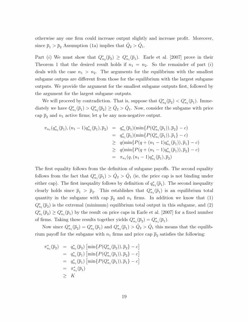
Part (i) We must show that Q∗n2(p2) ≥ Q∗n1
(p1). Earle et al. [2007] prove in their
Theorem 1 that the desired result holds if n1 = n2. So the remainder of part (i)
deals with the case n1 > n2. The arguments for the equilibrium with the smallest
subgame outpus are different from those for the equilibrium with the largest subgame
outputs. We provide the argument for the smallest subgame outputs first, followed by
the argument for the largest subgame outputs.
We will proceed by contradiction. That is, suppose that Q∗n2(p2) < Q∗n1
(p1). Imme-
diately we have Q∗n1(p1) > Q∗n2
(p2) ≥ Q̂2 > Q̂1. Now, consider the subgame with price
cap p2 and n1 active firms; let q be any non-negative output.
πn1(q∗n1
(p1), (n1 − 1)q∗n1(p1), p2) = q∗n1
(p1)(min{P (Q∗n1(p1)), p2} − c)
= q∗n1(p1)(min{P (Q∗n1
(p1)), p1} − c)≥ q(min{P (q + (n1 − 1)q∗n1
(p1)), p1} − c)≥ q(min{P (q + (n1 − 1)q∗n1
(p1)), p2} − c)= πn1(q, (n1 − 1)q∗n1
(p1), p2)
The first equality follows from the definition of subgame payoffs. The second equality
follows from the fact that Q∗n1(p1) > Q̂2 > Q̂1 (ie, the price cap is not binding under
either cap). The first inequality follows by definition of q∗n1(p1). The second inequality
clearly holds since p1 > p2. This establishes that Q∗n1(p1) is an equilibrium total
quantity in the subgame with cap p2 and n1 firms. In addition we know that (1)
Q∗n1(p2) is the extremal (minimum) equilibrium total output in this subgame, and (2)
Q∗n1(p2) ≥ Q∗n1
(p1) by the result on price caps in Earle et al. [2007] for a fixed number
of firms. Taking these results together yields Q∗n1(p2) = Q∗n1
(p1).
Now since Q∗n1(p2) = Q∗n1
(p1) and Q∗n1(p1) > Q̂2 > Q̂1 this means that the equilib-
rium payoff for the subgame with n1 firms and price cap p2 satisfies the following:
π∗n1(p2) = q∗n1
(p2)[min{P (Q∗n1
(p2)), p2} − c]
= q∗n1(p1)
[min{P (Q∗n1
(p1)), p2} − c]
= q∗n1(p1)
[min{P (Q∗n1
(p1)), p1} − c]
= π∗n1(p1)
≥ K
19

But this contradicts the fact that n2 < n1 is the equilibrium number of entering firms
when the price cap is p2; the subgame equilibrium payoff for n1 firms and price cap p2
must be less than K. So we have the result, Q∗n2(p2) ≥ Q∗n1
(p1).
The argument above explicity relies on the fact that the equilibrium under consid-
eration is the smallest equilibrium output level. We now provide an alternative proof
of this result for the largest equilibrium output level. As before, let p1 > p2. Let Q∗n(p)
be the maximal equilibrium output when the cap is p and n firms are active. We aim
to show that Q∗n2(p2) ≥ Q∗n1
(p1). We will proceed by contradiction. So, assume that
Q∗n2(p2) < Q∗n1
(p1). Immediately we have that Q̂1 < Q̂2 ≤ Q∗n2(p2) < Q∗n1
(p1)
Claim. Q∗n1(p2) is an equilibrium output level in the subgame with n1 firms and price
cap p1
Proof of Claim: All subgames dealt with in this Claim have n1 firms; so n = n1 and
we drop the n subscript in the proof of the Claim. We proceed by contradiction. So,
suppose Q∗(p2) is not an equilibrium in the subgame with cap p1 and n1 firms. By EST
it must be that Q∗(p2) > Q∗(p1). Let y∗(pk) ≡ (nk − 1)q∗(pk). Now, as in the proof of
Lemma 3.1, let π̃(Q, y, p) ≡ (Q−y)[min{P (Q), p}− c]. We may again think of a single
firm choosing total output, Q, when the other n1 − 1 firms choose y. Let Q(y, p) be
the maximal selection from the best response for a firm when the total output of the
other n1 − 1 firms is y and the price cap is p.
Since Q∗(p2) is not an equilibrium in the subgame with cap p1 and n1 firms, we
have:
π̃(Q∗(p2), y∗(p2), p1) < π̃(Q(y∗(p2), p1), y
∗(p2), p1) (6)
The inequality Q∗(p1) < Q∗(p2) implies that y∗(p1) < y∗(p2). Recall from the proof
of Lemma 3.1 that Q(y, p) is nondecreasing in y for fixed p. Hence, we must have
Q(y∗(p1), p1) ≤ Q(y∗(p2), p1). But since Q∗(p1) is maximal subgame equilibrium total
output, we must have Q(y∗(p1), p1) = Q∗(p1). Hence:
Q∗(p1) ≤ Q(y∗(p2), p1) (7)
Recall that Q̂1 < Q̂2 < Q∗(p1) < Q∗(p2). Equation (7) therefore implies Q̂1 < Q̂2 <
Q(y∗(p2), p1). But then (6) implies,
π̃(Q∗(p2), y∗(p2), p2) < π̃(Q(y∗(p2), p1), y
∗(p2), p2)
20

since neither cap binds under either output level. The above equation contradicts the
definition of Q∗(p2) . Hence, the claim is established.
The Claim establishes that Q∗n1(p2) is an equlibrium total output for the subgame
with n1 firms and cap p1. This output cannot exceed maximal equilibrium output for
this subgame, so Q∗n1(p2) ≤ Q∗n1
(p1). By Theorem 1 in EST, we must have Q∗n1(p2) ≥
Q∗n1(p1). Combining these two inequalities yields, Q∗n1
(p2) = Q∗n1(p1). As in the proof
for the minimal equilibrium output level, we can use this equality to show that n1
firms would have an incentive to enter when the cap is p2, contradicting the condition
n1 > n2.
Part (ii) Let W (p) be total welfare in the equilibrium with the lowest output when the
price cap is p. Let Q∗i = Q∗ni(pi), i ∈ {1, 2}. Now note:
W (p2) =∫ Q∗20
[P (z)− c] dz − n2K
≥∫ Q∗20
[P (z)− c] dz − n1K
≥∫ Q∗10
[P (z)− c] dz − n1K
= W (p1)
The first inequality follows since n1 ≥ n2. The second inequality follows from the fact
that Q∗2 ≥ Q∗1 and that P (Q∗2) ≥ c (otherwise any firm could increase its period two
profit by reducing output).
Part (iii) Let CS(Q, p) denote consumer surplus when total production is Q and the
price cap is p.
CS(Q, p) =
∫ Q
0
[P (z)−min{P (Q), p}] dz
Note that CS(Q, p) is increasing in Q and is decreasing in p. Since Q∗n2(p2) ≥ Q∗n1
(p1)
and p2 < p2, immediately we have that CS(Q∗n2(p2), p2) ≥ CS(Q∗n1
(p1), p1).
Proof of Proposition 2
Let p < P (Q∞) such that p ∈ P. We first claim that equilibrium output under the cap
satisfies P (Q∗(p)) = p.
To establish the claim we proceed by contradiction. So, suppose not. Then we
must have P (Q∗(p)) < p or equivalently, Q∗(p) > Q̂(p). Now, consider the subgame
21

with no cap and n∗ firms. Since n∗ ≤ n∞ it must be that Q∞n∗ ≤ Q∞ < Q̂. It follows
that Q∗(p) > Q̂ > Q∞n∗ .
Let π̃L(Q, y) ≡ ln(π̃(Q, y)). Where π̃(Q, y) = (Q − y)(P (Q) − c). Note that since
P is log-concave this implies π̃L is strictly concave in Q for all Q such that P (Q) > c.
Let Q(y) ≡ arg maxQ≥y π̃L(Q, y). Since π̃L is strictly concave in Q, clearly Q(y) is a
single-valued function. In the subgame with n∗ firms and no cap, using standard results,
we must have a unique equilibrium since P is log-concave. This means Q∗(p) cannot be
an equilibrium output level with no cap and n∗ firms. Let y∗(p) =(n∗−1n∗
)Q∗(p). Then
since Q∗(p) is not an equilibrium output in the absence of a price cap it follows that
Q(y∗(p)) 6= Q∗(p). In particular, it must be that Q(y∗(p)) < Q̂ < Q∗(p). If Q(y∗(p)) ≥Q̂ then Q(y∗(p)) would also be the best response to y∗(p) under the price cap as well.
This would contradict the definition of Q∗(p). Then since in any equilibrium price
must be strictly above marginal cost, the strict concavity of π̃L implies:
π̃L(Q(y∗(p)), y∗(p)) > π̃L(Q̂, y∗(p)) > π̃L(Q∗(p), y∗(p))
This implies that π̃(Q̂, y∗(p)) > π̃(Q∗(p), y∗(p)). But since P (Q̂) = p and P (Q∗(p)) < p,
we have:
(Q̂− y∗(p))(min{P (Q̂), p} − c) > (Q∗(p)− y∗(p))(min{P (Q∗(p), p} − c)
This contradicts the definition of Q∗(p) and establishes the claim. Now under any
relevant cap, equilibrium output must satisfy P (Q∗(p)) = p. Clearly, this means there
may exist only one symmetric equilibrium.
Consider two caps p2 < p1 < P (Q∞) such that pi ∈ P for each i ∈ {1, 2}. By
the claim established in the first part of the proof, we must have p1 = P (Q∗(p1)) >
P (Q∗(p2)) = p2. Obviously, since P is strictly decreasing Q∗(p1) < Q∗(p2) The result
is immediate.
Proof of Proposition 3
As in Proposition 1, Assumption (1b) implies that each firm’s output choice can be
restricted to a convex set, [0,M ], for some large positive M . We refer to the original
game as the n player game in which each firm chooses output q from [0,M ] to maximize
π(q, y, p), where y is total output of rivals. However, a formulation of the output choice
game with this choice set implies a payoff function that does not satisfy SCP in (q,−p).
22

Define q̂ ≡ C ′−1(p̂), and consider a modified game in which each firm’s output choice
is restricted to [0, q̂].
Claim 1: An output level q′ is a symmetric Nash equilibrium of the original game if
and only if it is a symmetric Nash equilibrium of the modified game.
(⇐) Let q∗∗ be a symmetric Nash equilibrium of the original game. Suppose that
q∗∗ > q̂. Then C ′(q∗∗) > p̂ since C ′(·) is strictly increasing. Also, P (nq∗∗) < P (nq̂) = p̂
since P (·) is strictly decreasing. We have the following payoff relationships:
π(q∗∗, (n− 1)q∗∗, p) = q∗∗min{P (nq∗∗), p} − C(q∗∗)
= q∗∗P (nq∗∗)− C(q∗∗)
≤ q̂P (nq∗∗)− C(q̂)
< q̂P (q̂ + (n− 1)q∗∗)− C(q̂)
= q̂min{P (q̂ + (n− 1)q∗∗), p} − C(q̂)
= = π(q̂, (n− 1)q∗∗, p)
The first equality is definitional. The second equality holds since P (nq∗∗) < p̂. The
first inequality holds since P (nq) < C ′(q) for all q ∈ [q̂, q∗∗]. The second inequality
holds since P (·) is strictly decreasing and q̂ < q∗∗. The next equality holds since
P (q̂ + (n− 1)q∗∗) < p̂ ≤ p, and the final equality holds by the definition of the payoff
function. These inequalities establish that q∗∗ is not a best response to y = (n− 1)q∗∗
and so q∗∗ cannot be a symmetric Nash equilibrium output. The supposition that
q∗∗ > q̂ has led to a contradiction; if q∗∗ is a symmetric Nash equilibrium of the original
game then q∗∗ ≤ q̂. From this it follows that q∗∗ is a symmetric Nash equilibrium of
the modified game.
(⇒) Let q∗ be a symmetric Nash equilibrium of the modified game and let q∗∗ be a
symmetric Nash equilibrium of the original game. Suppose that q∗ is not a symmetric
Nash equilibrium of the original game. Then there exists q̃ > q̂ such that,
π(q̃, (n− 1)q∗, p) > π(q∗, (n− 1)q∗, p) (8)
Since q̃ is a feasible choice for the original game, and q∗∗ is an equilibrium output for
the original game, we have:
π(q∗∗, (n− 1)q∗∗, p) ≥ π(q̃, (n− 1)q∗∗, p) (9)
23

And, since q∗∗ ≤ q̃ (established in proving the only-if part of the Claim) and therefore
a feasible choice for the modified game, we have:
π(q∗, (n− 1)q∗, p) ≥ π(q∗∗, (n− 1)q∗, p) (10)
Combining inequalities (8) - (10) yields,
π(q̃, (n−1)q∗, p)−π(q̃, (n−1)q∗∗, p) > 0 ≥ π(q∗∗, (n−1)q∗, p)−π(q∗∗, (n−1)q∗∗, p) (11)
Recall that for any q and any p, π(q, y, p) is non-increasing in y. Then the left-hand
side of (11) implies that (n−1)q∗ < (n−1)q∗∗, while the right-hand side of (11) implies
that (n − 1)q∗ ≥ (n − 1)q∗∗ which is a contradiction. Hence, it must be that q∗ is an
equilibrium output choice of the original game. This demonstrates Claim 1.
Claim 2: The payoff function π(q, y, p) for the modified game satisfies the single cross-
ing property (SCP) in (q,−p) for all y ≥ 0.
Proof of Claim 2: Let p′ > p > p̂ and let q < q′ ≤ C′−1(p̂). Assume that π(q′, y, p′) >
π(q, y, p′). We will show that this implies π(q′, y, p) > π(q, y, p). To do this, we will
seperately examine three cases.
(a) First, suppose that the price cap p binds for both quantities q and q′. Then since
p > p̂ immediately it must be that C′(q) < C
′(q′) ≤ p̂ < p. Hence, π(z, y, p) =
zp − C(z) is strictly increasing in z for all z ∈ [q, q′]. This immediately implies
that π(q′, y, p) > π(q, y, p)
(b) Next, suppose that the price cap, p binds for q but not for q′. Since, the lower cap
does not bind for output q′, the higher cap must not have been binding either. So,
π(q′, y, p) = π(q′, y, p′) > π(q, y, p′) ≥ π(q, y, p).
(c) If the cap does not bind for either quantity, then the profits are the same under p
as they were under p′. This establishes Claim 2.
The arguments that establish that total output in symmetric equilibria of the mod-
ified game with the smallest and largest outputs are nonincreasing in the price cap are
analogous to the arguments used in Earle et al. [2007] in their proof of Theorem 1;
because the arguments are so similar to those in Earle et al., we do not include them
here. These arguments rely on the payoff function satisfying SCP in (q,−p). Our
24
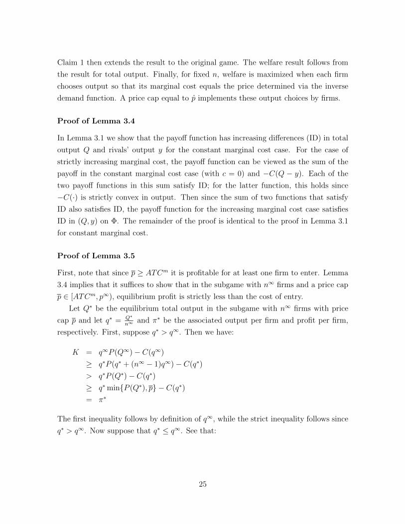
Claim 1 then extends the result to the original game. The welfare result follows from
the result for total output. Finally, for fixed n, welfare is maximized when each firm
chooses output so that its marginal cost equals the price determined via the inverse
demand function. A price cap equal to p̂ implements these output choices by firms.
Proof of Lemma 3.4
In Lemma 3.1 we show that the payoff function has increasing differences (ID) in total
output Q and rivals’ output y for the constant marginal cost case. For the case of
strictly increasing marginal cost, the payoff function can be viewed as the sum of the
payoff in the constant marginal cost case (with c = 0) and −C(Q − y). Each of the
two payoff functions in this sum satisfy ID; for the latter function, this holds since
−C(·) is strictly convex in output. Then since the sum of two functions that satisfy
ID also satisfies ID, the payoff function for the increasing marginal cost case satisfies
ID in (Q, y) on Φ. The remainder of the proof is identical to the proof in Lemma 3.1
for constant marginal cost.
Proof of Lemma 3.5
First, note that since p ≥ ATCm it is profitable for at least one firm to enter. Lemma
3.4 implies that it suffices to show that in the subgame with n∞ firms and a price cap
p ∈ [ATCm, p∞), equilibrium profit is strictly less than the cost of entry.
Let Q∗ be the equilibrium total output in the subgame with n∞ firms with price
cap p and let q∗ = Q∗
n∞and π∗ be the associated output per firm and profit per firm,
respectively. First, suppose q∗ > q∞. Then we have:
K = q∞P (Q∞)− C(q∞)
≥ q∗P (q∗ + (n∞ − 1)q∞)− C(q∗)
> q∗P (Q∗)− C(q∗)
≥ q∗min{P (Q∗), p} − C(q∗)
= π∗
The first inequality follows by definition of q∞, while the strict inequality follows since
q∗ > q∞. Now suppose that q∗ ≤ q∞. See that:
25

K = q∞P (Q∞)− C(q∞)
≥ q∗P (Q∞)− C(q∗)
> q∗p− C(q∗)
≥ q∗min{P (Q∗), p} − C(q∗)
= π∗
To see why the first inequality holds, note that Q∞ must satisfy P (Q∞) ≥ C ′(q∞).
Since C ′(·) is strictly increasing, we must have P (Q∞) > C ′(x) for all x ∈ [0, q∞).
Hence, the function xP (Q∞) − C(x) is strictly increasing in x for x ∈ [0, q∞). Since
q∗ ≤ q∞, the inequality holds. Finally, note that the strict inequality follows since
p < P (Q∞).
Hence, we must have π∗ < K.
Proof of Proposition 4
First note that since the entry constraint is binding, by Lemma 3.5 any price cap,
p ∈ [ATCm, p∞), results in the entrance of at least one firm and at most n∞− 1 firms.
First, consider the subgame with n∞− 1 firms under a price cap p ∈ [ATCm, p∞). We
will then show that maximal equilibrium profit in this subgame is at least as large as
the cost of entry.
Let π(Q, y, p) = (Q−y) min{P (Q), p}−C(Q−y) be profit for a firm if total output
is Q, rivals’ output is y, and the price cap is p ∈ [ATCm, p∞). Initially we suppose
that y = (n∞ − 2)C ′−1(p); that is, each rival firm sets its output such that marginal
cost is equal to the price cap. Note that π(Q, y, p) is continuous in Q. Also
∂π(Q, y, p)
∂Q=
{p− C ′(Q− y), Q < P−1(p)
P (Q)− (Q− y)P ′(Q)− C ′(Q− y), Q > P−1(p)
For Q > P−1(p) we have the following inequalities:
∂π(Q, y, p)
∂Q< p− C ′(Q− y) < 0, (12)
where the first inequality follows because the inverse demand function is strictly de-
creasing in Q. The second inequality is due to the following argument. First, the
assumption that C ′( Q∞
n∞−1) > p∞ implies that, Q∞ > (n∞ − 1)C ′−1(p∞) ≥ (n∞ −1)C ′−1(p) = y + C ′−1(p). Second, Q > P−1(p) implies Q > Q∞ so, Q − y > C ′−1(p).
Third, this implies that p− C ′(Q− y) < 0, which is the second inequality in equation
26

(12) above.
Since the payoff function is strictly decreasing in Q for Q > P−1(p), it must be
that the best response Q to y is in the interval, [y, P−1(p)]. Strict convexity of the cost
function implies that the payoff function is strictly concave in Q in this interval. The
unique best response to y satisfies, p = C ′(Q − y); that is, it is optimal for a firm to
set its output such that marginal cost is equal to the price cap when each of its rivals
follows the same policy. The optimal choice of Q is in the interior of [y, P−1(p)] since
(by assumption) C ′( Q∞
n∞−1) > p∞. q∗ = C ′−1(p) is equilibrium output per firm in the
subgame with n∞− 1 firms. A proof-by-contradiction can be used to show that this is
the unique subgame equilibrium. Equilibrium profit is given by π∗(p) = q∗p− C(q∗)
To demonstrate (i), we show that in the subgame with n∞ − 1 firms for all p ∈[ATCm, p∞) we have π∗(p) ≥ K. Let qm solve minxATC(x). Then see that:
π∗(p) = q∗p− C(q∗)
≥ qmp− C(qm)
≥ qmATCm − C(qm) = K
The first inequality follows by the optimality of q∗ and the second follows since p ≥ATCm. Hence, the equilibrium number of firms is n∞−1. Then since C ′′ > 0, we have
that q∗ is increasing in p. Moreover, since p < p∞, we must have P((n∞ − 1)C
′−1(p))>
P((n∞ − 1)C
′−1(p∞))> p∞. So, (n∞ − 1)C
′−1(p) < Q∞. This establishes (i)− (iii).
Finally, note that for any relevant cap, equilibrium welfare is given by:
W ∗(p) =
∫ (n∞−1)C′−1(p)
0
P (z) dz − (n∞ − 1)C(C′−1(p))− (n∞ − 1)K
Now see that
W ∗′(p) =n∞ − 1
C ′′(C ′−1(p))
[P(
(n∞ − 1)C′−1(p)
)− p]> 0
,
which establishes (iv).
Proof of Lemma 4.1
As in Lemma 3.1 we define a firm’s payoff function in terms of total output Q and
rivals’ output y:
27

π̃(Q, y, p) = E [(Q− y) min{P (Q, θ), p} − (Q− y)c]
Let θb(Q, p) satisfy P (Q, θb(Q, p)) = p. So when total output is Q and the cap is p the
price cap will bind for shocks θ ≥ θb(Q, p). Now define
P̃ (Q, p) = E[min{P (Q, θ), p}] =
∫ θb(Q,p)
θ
P (Q, θ) dF (θ) +
∫ θ
θb(Q,p)
p dF (θ)
Since f(θ) > 0 for all θ ∈ (θ, θ], and andP1(Q, θ) < 0 for all Q ≥ y, θ ∈ Θ we have:
P̃1(Q, p) =
∫ θb(Q,p)
θ
P1(Q, θ) dF (θ) ≤ 0
Then π̃(Q, y, p) = (Q−y)(P̃ (Q, p)− c
). The cross partial derivative of π̃ with respect
to Q and y on Φ is given by −P̃1(Q, p) ≥ 0. This establishes that π̃ has ID in (Q, y)
on Φ. The remainder of the proof is analogous to Lemma 3.1.
Proof of Proposition 5
For notational convenience, in this proof we let n∞ ≡ n. Concavity of p(·) implies the
existence of a unique symmetric period two subgame equilibrium. Also, concavity of
p(·) implies that, for a fixed number of firms, equilibrium profit is continuous in the
price cap. If π∞ > K then by the continuity of period two profit in p, there is an
interval of price caps below ρn such that the equilibrium number of entrants remains
at n. For a fixed number of firms, Grimm and Zottl [2010] establish that any price
cap p ∈ [MRn, ρn) both increases output and total welfare. Thus, a price cap in the
intersection of [MRn, ρn) and the set of price caps for which n firms enter will leave
the equilibrium number of firms unchanged and will increase both output and welfare.
If π∞ = K then there exists a range of price caps below ρ∞ such that the equilibrium
number of firms decreases by exactly one. Also, if π∞ = K then by Assumption (1d)
we must have n ≥ 2. We let Qm denote equilibrium total output in the absence of a
price cap when m firms enter in the first stage. We also define per-firm output and
profit analogously. We begin by demonstrating that πn−1 > K.
In a subgame with no cap and m firms, the symmetric equilibrium condition is
given by:
28
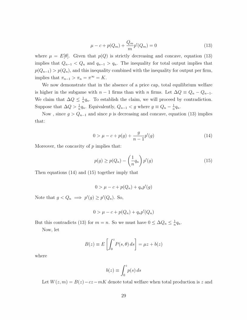
µ− c+ p(Qm) +Qm
mp′(Qm) = 0 (13)
where µ = E[θ]. Given that p(Q) is strictly decreasing and concave, equation (13)
implies that Qn−1 < Qn and qn−1 > qn. The inequality for total output implies that
p(Qn−1) > p(Qn), and this inequality combined with the inequality for output per firm,
implies that πn−1 > πn = π∞ = K.
We now demonstrate that in the absence of a price cap, total equilibrium welfare
is higher in the subgame with n − 1 firms than with n firms. Let ∆Q ≡ Qn − Qn−1.
We claim that ∆Q ≤ 1nqn. To establish the claim, we will proceed by contradiction.
Suppose that ∆Q > 1nqn. Equivalently, Qn−1 < g where g ≡ Qn − 1
nqn.
Now , since g > Qn−1 and since p is decreasing and concave, equation (13) implies
that:
0 > µ− c+ p(g) +g
n− 1p′(g) (14)
Moreover, the concavity of p implies that:
p(g) ≥ p(Qn)−(
1
nqn
)p′(g) (15)
Then equations (14) and (15) together imply that
0 > µ− c+ p(Qn) + qnp′(g)
Note that g < Qn =⇒ p′(g) ≥ p′(Qn). So,
0 > µ− c+ p(Qn) + qnp′(Qn)
But this contradicts (13) for m = n. So we must have 0 ≤ ∆Qn ≤ 1nqn.
Now, let
B(z) ≡ E
[∫ z
0
P (s, θ) ds
]= µz + b(z)
where
b(z) ≡∫ z
0
p(s) ds
Let W (z,m) = B(z)−cz−mK denote total welfare when total production is z and
29

m firms enter. Let ∆W ≡ W (Qn−1, n−1)−W (Qn, n) denote the change in equilibrium
welfare when the number of firms decreases by one in the absence of a cap. Note that
πn = K implies that
∆W = − [B(Qn)−B(Qn−1)− (∆Qn)c] + πn
Note that the term in square brackets above is given by
(µ− c)∆Q+
∫ Qn
Qn−1
p(s) ds
Now, let T (s;x) = p′(x)s + p(x) − p′(x)x denote the equation of the line tangent
to p at output x. Note that since p is concave and decreasing, for all s ∈ [Qn−1, Qn],
p(s) ≤ T (s,Qn). This means∫ Qn
Qn−1
p(s) ds ≤∫ Qn
Qn−1
T (s;Qn) ds = ∆Qp(Qn)− 1
2(∆Q)2p′(Qn)
Plugging this back into the expression for ∆W we see that:
∆W ≥ 1
2p′(Qn)(∆Qn)2 − (p(Qn) + µ− c) ∆Q+ πn
Then, from (13), it follows that p(Qn) + µ − c = −p′(Qn)qn and πn = −p′(Qn)(qn)2.
Combining this with the fact that ∆Q ≤ 1nqn, p′ < 0 and n ≥ 2 yields:
∆W ≥ 12p′(Qn)(∆Q)2 + p′(Qn)qn∆Q− p′(Qn)(qn)2
≥ 12p′(Qn)( 1
nqn)2 + p′(Qm) 1
n(qn)2 − p′(Qn)(qn)2
= p′(Qn)q2n(
12n2 + 1
n− 1)> 0
Thus we see that, in the absence of a price cap total welfare increases when the num-
ber of firms that enter decreases by one. Let MRm denote the maximal equilibrium
marginal revenue when m firms enter and there is no price cap. Clearly, by assumptions
placed on P ,
MRm = θ + p(Q∞m ) + p′(Q∞m )q∞m
30

By the first order equilibrium conditions, it follows that p(Q∞m ) + p′(Q∞m )q∞m = c − µ.
Hence, independent of m it is clear that
MRm = θ + c− µ
and since p′ < 0:
MRm < θ + p(Q∞m ) = ρm
Since MRm is independent of m, we drop this subscript and write MR. Let ρm =
P (Q∞m , θ). Now, since π∞ = K and πn−1 > K, there exists a range of price caps strictly
less than ρn such that the equilibrium number of firms will decrease by exactly one12.
Let p̂1 denote the smallest of these price caps. Let p̂ ≡ max{p̂1,MR}. Then since
MR < ρn and p̂1 < ρn we have p̂ < ρn. Also see that under any price cap p ∈ [p̂, ρn)
the equilibrium number of firms is n− 1. Finally note that by lemma (4.1) it is clear
that ρn ≤ ρn−1.
Choose p ∈ [p̂, ρn). Then since p ∈ [MR, ρn−1) by Grimm and Zottl [2010] Theo-
rem 1, it follows that equilibrium welfare under the price cap is strictly greater than
equilibrium welfare in the subgame with n− 1 firms and no cap. Since welfare in the
absence of a cap when n − 1 firms enter is strictly higher than welfare when n firms
enter, the result follows.
Proof of Lemma 4.2
Recall that the necessary condition for equilibrium capacities is:
∫ θ
θ̃(Xn)
[ θ + p(Xn) + xnp′(Xn)] dF (θ) = c (16)
By the definition of θ̃(Xm) and θ̃(Xn) this necessary condition may be re-written as:
∫ θ
θ̃(Xm)
[θ − θ̃(Xm)
]dF (θ) =
∫ θ
θ̃(Xn)
[θ − θ̃(Xn)
]dF (θ) = c
Let G(s) =∫ θs[θ − s ]dF (θ) and note that G′(s) =
∫ θs−1 dF (θ). Note that G′(s) < 0
for all s < θ. Then, the first-order conditions imply that G(θ̃(Xm)) = G(θ̃(Xn)). Since
12Once again, this follows since concavity of P implies the continuity of equilibrium profit in theprice cap
31

θ̃(Xm) < θ and θ̃(Xn) < θ it must be that θ̃(Xm) = θ̃(Xn).
Proof of Lemma 4.3
By Lemma 4.2 it follows that θ̃(Xn) = θ̃(Xn−1) = θ̃. First, fix θ < θ̃. In this case we
have Qn(θ) = Q̃n(θ) and Qn−1(θ) = Q̃n−1(θ). Both output choices must satisfy their
respective first-order conditions:
θ + p(Q̃n(θ)) + q̃n(θ)p′(Q̃n(θ)) = 0
and
θ + p(Q̃n−1(θ)) + q̃n−1(θ)p′(Q̃n−1(θ)) = 0
From the first-order conditions, the concavity of p together with the fact that p′ < 0
implies that Q̃n(θ) > Q̃n−1(θ) and q̃n(θ) < q̃n−1(θ)
Now, since θ̃(Xn) = θ̃(Xn−1) = θ̃ it follows from the definitions of θ̃(Xn) and
θ̃(Xn−1) that
θ̃ + p(Xn) + xnp′(Xn) = 0
and
θ̃ + p(Xn−1) + xn−1p′(Xn−1) = 0
Once again, these equations together with our assumptions on p ensure that Xn > Xn−1
and xn < xn−1. This establishes (i) and (ii).
Note that the first-order condition given in (16) implies that(∫ θ
θ̃(Xn−1)
[θ + p(Xn−1) ]dF (θ)− c
)> 0 (17)
Then by parts (i) and (ii) above, we have:
32

πn−1 =∫ θ̃(Xn−1)
θq̃n−1(θ)[θ + p(Q̃n−1(θ))] dF (θ) + xn−1
(∫ θθ̃(Xn−1)
[θ + p(Xn−1) ]dF (θ)− c)
>∫ θ̃(Xn)
θq̃n(θ)[θ + p(Q̃n−1(θ))] dF (θ) + xn
(∫ θθ̃(Xn)
[θ + p(Xn−1) ]dF (θ)− c)
>∫ θ̃(Xn)
θq̃n(θ)[θ + p(Q̃n(θ))] dF (θ) + xn
(∫ θθ̃(Xn)
[θ + p(Xn) ]dF (θ)− c)
= πn
The first inequality holds since θ̃(Xn−1) = θ̃(Xn), q̃n−1 > q̃n, xn−1 > xn and (17).
The second inequality holds since Q̃n > Q̃n−1 and Xn > Xn−1.
Proof of Proposition 6
As in the proof of Proposition 4, we demonstrate our result by showing that welfare in
the subgame with n firms and no price cap is strictly lower than welfare in the subgame
with n − 1 firms and no cap. For each θ ∈ Θ let ∆Q(θ) ≡ Qn(θ) − Qn−1(θ). We will
first demonstrate that for each θ, ∆Q(θ) ≤ 1nqn(θ).
Using the fact that θ̃(Xn) = θ̃(Xn−1) we first examine the case when θ < θ̃. In this
case, we use the first order conditions and the proof is identical to the proof in the
previous section. For the case when θ > θ̃ we again use the definition of θ̃ and follow
a similar argument as in the previous section.
Thus, for each θ ∆Q(θ) ≤ 1nqn(θ)
Now, let Wm denote equilibrium expected welfare in the subgame with m firms.
Let ∆W ≡ Wn−1 −Wn. Note that
Wn = E
[∫ Qn(θ)
0
[θ + p(s) ]ds
]− cXn − nπn
Which may be written:
Wn =
∫ θ̃
θ
[∫ Q̃n(θ)
0
[θ + p(s) ]ds
]dF (θ) +
∫ θ
θ̃
[∫ Xn
0
[θ + p(s)] ds
]dF (θ)− cXn − nπn
Let ∆W = Wn−1 −Wn and note that
33

∆W = −∫ θ̃
θ
[∫ Q̃n(θ)
Q̃n−1(θ)
[θ + p(s) ]ds
]dF (θ)−
∫ θ
θ̃
[∫ Xn
Xn−1
[θ + p(s)] ds
]dF (θ)+(∆X)c+πn
Now, following a similar argument as in the previous section, using the concavity
of p, we may show that for each θ ∈ [θ, θ̃]
∫ Q̃n(θ)
Q̃n−1(θ)
[θ + p(s) ]ds ≤ ∆Q̃(θ)(θ + p(Q̃n(θ)))− 1
2(∆Q̃(θ))2p′(Q̃n(θ)) ≡ A(θ)
Moreover, for each θ ∈ [θ̃, θ]∫ Xn
Xn−1
[θ + p(s) ]ds ≤ ∆X(θ + p(Xn))− 1
2(∆X)2p′(Xn) ≡ B(θ)
Now, using the first-order conditions we may write:
πn =
(−∫ θ̃
θ
(q̃n(θ))2p′(Q̃n(θ)) dF (θ)
)+
(−∫ θ
θ̃
(xn)2p′(Xn) dF (θ)
)≡ πAn + πBn
Hence, it follows that
∆W ≥ −∫ θ̃
θ
A(θ) dF (θ)−∫ θ
θ̃
B(θ) dF (θ) + (∆X)c+ πAn + πBn
Now, note that
−∫ θ̃
θ
A(θ) dF (θ)+πAn =
∫ θ̃
θ
[−∆Q̃(θ)(θ + p(Q̃n(θ))) +
1
2(∆Q̃(θ))2p′(Q̃n(θ))− (q̃n(θ))2p′(Q̃n(θ))
]dF (θ)
Using the first-order conditions once again, we know that for each θ ∈ [θ, θ̃] it holds
that θ+ Q̃n = −q̃n(θ)p′(Q̃n). This, combined with the fact that ∆Q̃(θ) ≤ 1nq̃n(θ) allow
us to write
34

−∫ θ̃
θ
A(θ) dF (θ) + πAn ≥∫ θ̃
θ
(q̃n(θ)p′(Q̃n(θ))
(1
n+
1
2n2− 1
)dF (θ) > 0
Now also see that
−∫ θθ̃B(θ) dF (θ) + (∆X)c+ πBn
= −∆X[∫ θ
θ̃(θ + p(Xn)) dF (θ)− c
]+∫ θθ̃
[12(∆X)2p′(Xn)− (xn)2p′(Xn)
]dF (θ)
From the first-order condition, it follows that
∫ θ
θ̃
(θ + p(Xn)) dF (θ)− c =
∫ θ
θ̃
−xnp′(Xn) dF (θ)
This, combined with the fact that ∆X ≤ 1nxn allows us to write:
−∫ θ
θ̃
B(θ) dF (θ) + (∆X)c+ πBn ≥ (xn)2p′(Xn)
∫ θ
θ̃
(1
n+
1
2n2− 1
)dF (θ) > 0
It follows immediately that ∆W > 0. The remainder of the proof works identically
to the proof of Proposition 5. The result follows.
References
Amir, R. and Lambson, V. (2000). On the effects of entry in Cournot markets. Review
of Economic Studies, 67.
Cottle, R. and Wallace, M. (1983). Economic effects of non-binding price constraints.
The Journal of Industrial Economics, 31(4):469–474.
Earle, R., Schmedders, K., and Tatur, T. (2007). On price caps under uncertainty.
Review of Economic Studies, 74:93–111.
Grimm, V. and Zottl, G. (2006). Capacity choice under uncertainty: The impact of
market structure. University of Cologne Working Paper Series in Economics, (23).
35

Grimm, V. and Zottl, G. (2010). Price regulation under demand uncertainty. The B.E.
Journal of Theoretical Economics, 10(1).
Mankiw, N. G. and Whinston, M. (1986). Free entry and social inefficiency. The Rand
Journal of Economics, 17(1):48–58.
Topkis, D. (1978). Minimizing a submodular function on a lattice. Operations Research,
26(2).
36
Recommended