Phase diagram of water between hydrophobic surfacesKenichiro Koga and Hideki Tanaka Citation: The Journal of Chemical Physics 122, 104711 (2005); doi: 10.1063/1.1861879 View online: http://dx.doi.org/10.1063/1.1861879 View Table of Contents: http://scitation.aip.org/content/aip/journal/jcp/122/10?ver=pdfcov Published by the AIP Publishing Articles you may be interested in Surface phase diagram and alloy formation for antimony on Au(110) J. Vac. Sci. Technol. A 26, 485 (2008); 10.1116/1.2905249 Surface freezing in normal alkanes: A statistical physics approach J. Chem. Phys. 124, 214906 (2006); 10.1063/1.2204036 Bilayer ice and alternate liquid phases of confined water J. Chem. Phys. 119, 1694 (2003); 10.1063/1.1580101 Solvation forces and liquid–solid phase equilibria for water confined between hydrophobic surfaces J. Chem. Phys. 116, 10882 (2002); 10.1063/1.1480855 Optical measurements of the phase diagrams of Langmuir monolayers of fatty acid, ester, and alcohol mixturesby Brewster-angle microscopy J. Chem. Phys. 106, 1913 (1997); 10.1063/1.473312

This article is copyrighted as indicated in the article. Reuse of AIP content is subject to the terms at: http://scitation.aip.org/termsconditions. Downloaded to IP:

130.113.111.210 On: Fri, 19 Dec 2014 22:13:35

Phase diagram of water between hydrophobic surfacesKenichiro Kogaa! and Hideki TanakaDepartment of Chemistry, Okayama University, Okayama 700-8530, Japan

sReceived 20 October 2004; accepted 3 January 2005; published online 14 March 2005d

Molecular dynamics simulations demonstrate that there are at least two classes ofquasi-two-dimensional solid water into which liquid water confined between hydrophobic surfacesfreezes spontaneously and whose hydrogen-bond networks are as fully connected as those of bulkice. One of them is the monolayer ice and the other is the bilayer solid which takes either acrystalline or an amorphous form. Here we present the phase transformations among liquid, bilayeramorphoussor crystallined ice, and monolayer ice phases at various thermodynamic conditions, thendetermine curves of melting, freezing, and solid-solid structural change on the isostress planeswhere temperature and intersurface distance are variable, and finally we propose a phase diagram ofthe confined water in the temperature-pressure-distance space. ©2005 American Institute ofPhysics. fDOI: 10.1063/1.1861879g

I. INTRODUCTION

Confined water has been less extensively studied thanbulk water but it is by no means less interesting or less rel-evant to us. Confined water exists in biological systemsscellmembranes, inner cavities of proteins, etc.d, geological ma-terials sclays, rocks, etc.d, and synthesized or industrial ma-terials sgraphitic microfibers with slit pore, inner space ofcarbon nanotubes, etc.d. Some biological systems becomeunstable or does not function if confined water is removed.Some important properties of nanostructured materials arehighly sensitive to the presence of confined water.

Phase behavior of a fluid is much richer in inhomoge-neous systems including confined systems than in the bulksystem: such nonbulk systems may exhibit confinement-induced freezing and melting, wetting and drying transitions,and prewetting and predrying transitions. Pioneering andmore recent theoretical studies of simple fluids are illuminat-ing in understanding those phenomena.1–3 Water is a com-plex fluid in the sense that its intermolecular interactioncauses hydrogen bonding and so is highly directional. There-fore its phase behavior in confined geometry can be evenmore complex than that expected from the intermolecularinteractions.

Computer simulation has proved to be a powerful theo-retical tool for studying such complex behavior of confinedwater. There are many computational studies on confinedwater,4–12 some of the pioneering works date back to 1980s.4

One of the earlier computer simulations focusing on liquid-solid phase transitions13 showed that water between hydro-phobic surfaces freezes into a bilayer form of crystalline icewhen temperature is lowered under a fixed normal pressure.Structure of the bilayer ice is different from any of the 12bulk ices but each molecule is hydrogen bonded to its fourneighbors as it is in the bulk ices. A few years later it wasshown that water confined in a rigid hydrophobic slit porefreezes into the bilayer amorphous solid when temperature is

decreased at a fixed lateral pressure.14 This phase change isunique in that freezing to and melting of the amorphous solidoccur as a first-order phase transition accompanying a largeamount of latent heat and structural change. This is an un-ambiguous demonstration of polyamorphism involving liq-uid water by computer simulation. The freezing and meltingare also observed by changing the distance between surfacesat fixed temperature and fixed lateral or bulk pressure, a re-sult of which is a discontinuous force curve with hysteresis.15

More recently spontaneous formation of a monolayer ice wasfound by molecular dynamicssMDd simulations of theTIP5P model water.16

Quasi-one-dimensional water, too, exhibits phase transi-tions qualitatively different from those of the bulk water. Thefirst evidence for such transitions was again obtained fromMD simulations combined with free-energy calculations: thesimulations demonstrated that water inside a carbon nano-tube freezes into four different forms of the ice nanotube, aclass of quasi-one-dimensional crystalline ices.17,18 The pre-dicted formation of the ice nanotube was confirmed by ex-periments of Maniwaet al.19

The structure, dynamics, and thermodynamic propertiesof confined water depend on many factors such as confininggeometry and physical and chemical properties of surfaces,and the effect of each factor is as yet little understood. Thusit is sensible to choose and study, among many possibilities,model systems with simpler geometriesse.g., slit and cylin-drical poresd and simpler surfacesse.g., structureless sur-facesd. Even such simpler systems give rise to at least oneadditional thermodynamic parameter for specifying a ther-modynamic state. Full understanding of the phase behaviorof confined water with a given geometry requires explorationof a three-dimensional thermodynamic spacese.g., theTPxspace, wherex is a geometrical parameter such as diameterof the pore or separation distance of two surfacesd. Here wefocus on the quasi-two-dimensional system and examine thephase behavior of water in ranges of the thermodynamic con-ditions much wider than we have done before.adElectronic mail: koga@cc.okayama-u.ac.jp

THE JOURNAL OF CHEMICAL PHYSICS122, 104711s2005d

0021-9606/2005/122~10!/104711/10/$22.50 © 2005 American Institute of Physics122, 104711-1

This article is copyrighted as indicated in the article. Reuse of AIP content is subject to the terms at: http://scitation.aip.org/termsconditions. Downloaded to IP:

130.113.111.210 On: Fri, 19 Dec 2014 22:13:35

II. SYSTEM AND CONDITIONS

As shown in Fig. 1, the model system comprisesN mol-ecules in a regular rectangular prism with the dimensionsLx3Ly3H in the x, y, andz directions. Periodic boundaryconditions are imposed on thex and y directions and twoparallel planner walls placed at the top and bottom faces ofthe prism confine all the molecules between them. The po-tential energyU of the system is defined as a sum of thepotential energy among water molecules and that of thewater-wall interaction, both being pair-wise additive:

U = oi=1

N−1

oj=i+1

N

fsr ijd + ok=1

2

oi=1

N

vszikd, s1d

where f is the TIP4P water potential20 multiplied by theswitching function that smoothly truncates the potential atrc=8.75 Å;21 its argumentr ij represents the relative configu-ration of moleculesi and j including their orientations. Thepair potentialv between moleculei and wallk is a functiononly of the distancezik from the wallsthe top or base face ofthe prismd to the position of the oxygen atom of the mol-ecule:

vszikd = C9/zik9 − C3/zik

3 . s2d

This Lennard-JonessLJd 9-3 potential22 results from the LJ12-6 potential integrated over infinite volume of each wallwith a uniform density. The parametersC9 andC3 are thosechosen for the interaction between a water molecule and a“hydrophobic” solid surface.5 The potential functionvszd iszero at the distancez0=sC9/C3d1/6=2.47 Å and rapidly in-creases at shorter distances. In Fig. 1 the dotted lines indicatethe surfaces of zero energyfvszd=0g with a distanceh apartwhereas the top and base faces of the prism indicate thesurfaces of infinite energy with a distanceH apart. NoteH−h=2z0. We takeh to be the effective width for water andV=Ah to be the effective volume of water, whereA=LxLy isthe area of the bases. Note that one must define, in one wayor the other, the effective width or volume as they are notuniquely defined for microscopic wall-wall separation. Withthe present definition of the effective widthh, water mayhave a monolayer structure ifh,0, a bilayer structure ifh,s, and so on, wheres is the molecular “diameter” ofwater.

MD simulations in the isothermal and isostress ensembleor NPxxs=PyydT ensemble are performed, wherePxx andPyy

are the components of pressure tensor normal to theyz andxz planes, respectively, to which we shall refer as the lateralpressure, andT is the temperature. This ensemble is not isos-

tress to the componentPzz of pressure tensor normal to thewalls, for the effective widthh is kept fixed. The isothermal-isostress MD simulation is more efficient than other MDsimulations in examining phase behavior and phase transi-tions of a liquid confined in a rigid slit pore. Implementationof theNPxxs=PyydT ensemble simulation is a straightforwardextension of the standard isothermal-isobaric MDsimulation;23 here the lateral dimensionsLx and Ly vary inresponse to the corresponding lateral pressures being keptfixed at a given value while the widthh is kept fixed.

A thermodynamic state of the one-component system isspecified by three variables, which are taken to beT, h, andPxx. Our main goal is to reveal the phase behavior of con-fined water in a part of the three-dimensional thermodynamicspace, in which both the bilayer and monolayer solid phasesare involved. To this end we choose two isostress planes,Pxx=200 MPa andPxx=0.1 MPa, and apply the MD simula-tion at thermodynamic states corresponding to grid points ofa square net within a rectangular region of 200KøTø270 K and 1.3 Åøhø6.0 Å for each isostress plane. Fig-ure 2 shows the two rectangular regions. Neighboring gridpoints are 0.1 Å or 0.2 Å apart forh and 5 or 10 K apart forT. In addition, thermodynamic states ath=7,8, . . . ,20 Å andat Pxx=0.1 MPa andT=200 K are examined.

The numberN of molecules is taken to be 240 for thestates withhø10 Å and 480 otherwise; then the lateral di-mensionsLx and Ly of the simulation box are larger than30 Å at any examined conditions. The Gear predictor-corrector method is employed for solving the equation ofmotion with a time step of 0.5 fs.

The following procedure is taken to determine the melt-ing and freezing curves on each of the two isostress planes.First we perform preliminary MD simulations to find outsome values ofh at which the liquid water spontaneouslyfreezes into the monolayer ice or into the bilayer amorphousice whenT decreases from 270 K to 200 K. Then we chooseone of such states as a starting pointse.g.,h=1.5 Å andT=200 K for the monolayer ice phased. Second we performMD simulations of 10 ns each at the neighboring grid pointsusing a final configuration of molecules at the starting pointand then check the structure, the potential energy, and otherproperties. In most cases it is easy to judge whether the sys-tem undergoes a phase change or remains in the same state at

FIG. 1. Schematic diagram of the system.

FIG. 2. Isostressh-T planes in which phase behavior of confined water isexamined.

104711-2 K. Koga and H. Tanaka J. Chem. Phys. 122, 104711 ~2005!

This article is copyrighted as indicated in the article. Reuse of AIP content is subject to the terms at: http://scitation.aip.org/termsconditions. Downloaded to IP:

130.113.111.210 On: Fri, 19 Dec 2014 22:13:35

a given condition; otherwise we extend the simulation up to100 ns at the same condition. The second step is repeated byencompassing the grid points until the solid phase melts ortransforms into the other solid phase. This set of MD simu-lations determines the melting curvesor the stability limitd ofthe solid phase. Once the melting curves are obtained it iseasy to find the freezing curves. The system in a liquid stateat the melting point at givenh is cooled by 5 K and is ex-amined if it freezes at that temperature within 20 ns. If thereis any sign of freezing the MD simulation is extended untilthe system freezes completely; if there is no sign of freezing,the temperature is further decreased in steps until spontane-ous freezing is observed. This set of MD simulations aredone at each value ofh in the grid points. At some values ofh the liquid water never freezes at and above 200 K. Thenthe value ofh is increased or decreased in steps at that tem-perature until the system freezes spontaneously. From theseMD simulations the freezing curves are determined at eachisostress plane.

It is worthwhile here to make some remarks on the em-ployment of the TIP4P model for water-water interaction andthe LJ 9-3 model for the water-wall interactions. The bilayerice and the bilayer amorphous have been obtained from thesimulations of the ST2 and TIP5P models.24 As mentionedearlier the monolayer ice has been obtained from the TIP5Pwater.16 The LJ 9-3 potential for the water-wall interactionignores any atomic structure of the walls, but it was con-firmed from our earlier simulations that a potential functionrepresenting structure of hydrophobic surfaces gives rise tothe same structure of the bilayer ice.sNote in the case thenormal pressure is fixed.d Therefore, the results presentedbelow would not be qualitatively altered by use of otherreasonable potential models for water and hydrophobic sur-faces.

III. THERMODYNAMICS FOR THE CONFINED SYSTEM

Thermodynamic identities for the one-component sys-tem having the quasi-two-dimensional geometry under theNPxxT ensemble are summarized here. For the thermody-namics of confined fluids in an open environment the readershould refer to the paper by Evans and Marini BettoloMarconi.1

The infinitesimal change in the internal energyU of theconfined systemfFig. 1g is written as

dU = TdS− APzzdh− PxxhdA+ mdN, s3d

and whenN, Pxx, h, andT are fixed the natural choice of thethermodynamic potential is

F = U + AhPxx − TS. s4d

Then its differential is given by

dF = − SdT− ADPdh+ AhdPxx + mdN, s5d

whereDP=Pzz−Pxx. From the general condition

dTdS− dsAPzzddh − dshPxxddA + dNdm ù 0 s6d

for the stability of this system, we find

s]APzz/]hdPxx+ Pxxs]A/]hdPxx

ø 0, s]A/]Pxxdh ø 0 s7d

with fixed T and N, in addition to s]S/]Tdh,Pxx,Nù0 and

s]m /]NdT,Pxx,hù0. These conditions determine the signs of

the second derivatives ofF:

]2F/]T2 ø 0, ]2F/]Pxx2 ø 0, ]2F/]N2 ù 0;

however they do not determine the sign of]2F /]h2 ors]ADP/]hdPxx

. Indeed, from the first inequality in Eq.s7d,

s]ADP/]hdPxxø − 2Pxxs]A/]hdPxx

,

the right-hand side of which can be either positive or nega-tive.

SinceF is a homogeneous first-order function ofN withfixed T, h, andPxx, integrating Eq.s5d gives

F = mN. s8d

This combined with Eq.s5d results in the Gibbs–Duhemequation for the confined system:

dm = − sdT− aDPdh+ vdPxx, s9d

where s=S/N, a=A/N, and v=Ah/N=V/N. Then we findfrom Eq. s9d the following Maxwell relations: for a fixedlateral pressurePxx,

S ]s

]hD

Pxx,T= S ]aDP

]TD

Pxx,h, s10d

for a fixed widthh,

S ]s

]PxxD

h,T= − S ]v

]TD

h,Pxx

, s11d

and for a fixed temperatureT,

S ]v]hD

T,Pxx

= − S ]aDP

]PxxD

T,h. s12d

Equilibrium conditions for any two distinct phasesa andbunder theNPxxT ensemble areTa=Tb, ma=mb, and Pxx

a

=Pxxb . Note that in generalPzz

a ÞPzzb at equilibrium.

A two-phase boundary of the present system is a surfacein the three-dimensional thermodynamic space, and theslopes of the surface at fixedh, T, andPxx are given, respec-tively, by

S ]T

]PxxD

h=

va − vb

sa − sb , s13d

S ]Pxx

]hD

T=

saDPda − saDPdb

va − vb , s14d

and

S ]h

]TD

Pxx

= −sa − sb

saDPda − saDPdb , s15d

which are the Clapeyron equations for the two-phase bound-aries in the quasi-two-dimensional system. The triple point atwhich three phasesa, b, andg are in equilibrium is a triple“line” in the three-dimensionals3Dd thermodynamic space.Sincedma=dmb anddmb=dmg along the triple line and each

104711-3 Phase diagram of water between hydrophobic surfaces J. Chem. Phys. 122, 104711 ~2005!

This article is copyrighted as indicated in the article. Reuse of AIP content is subject to the terms at: http://scitation.aip.org/termsconditions. Downloaded to IP:

130.113.111.210 On: Fri, 19 Dec 2014 22:13:35

dm is given by Eq.s9d, the direction of the triple line isuniquely determined. LetD1x andD2x denote the differencesxa−xb and xb−xg, respectively, for any quantityx of eachphase. Then the direction of the triple line is expressed as

dT

dPxx=

D1vD2saDPd − D2vD1saDPdD1sD2saDPd − D2sD1saDPd

s16d

and

dh

dPxx=

D1vD2s− D2vD1s

D1sD2saDPd − D2sD1saDPd. s17d

This is a set of Clapeyron equations for the triple line.The Clapeyron equations can be used to check the re-

sults of MD simulations and, when combined with them,provide an effective route to determination of the two-phaseboundaries and the triple line in the 3D thermodynamicspace.

IV. FORMATION AND STRUCTUREOF MONOLAYER ICE

Apart from a single MD simulation at each of the gridpoints to determine phase boundaries, ten independent MDsimulations at a representative thermodynamic pointsh=2.3 Å, T=250 K, andPxx=200 MPad are performed to ex-amine formation and structure of the monolayer ice. Initialconfigurations of water molecules are those of liquid water at270 K with the sameh and Pxx and a trajectory of 30 ns isgenerated in each simulation and if freezing is observed it isextended by 20 ns. It is found that the probability of freezinginto the monolayer ice within 30 ns is 80%. The phasechange accompanies significant decrease in the potential en-ergy. The average potential energy of the “metastable” liquidstate is −36.9 kJ/mol whereas that of the low-energy phaseis −41.6 kJ/mol.sThe latter value is the average over the last20 ns of a single trajectory of 50 ns.d The decrease in poten-tial energy, 4.7 kJ/mol, is as large as 80% of the latent heatof ice Ih.

The “lateral” radial distribution functionsgoosrds foroxygen atoms of the inherent structures are plotted in Fig. 3,wherer =ÎsDxd2+sDyd2 with Dx andDy being the differencein thex andy coordinates of two oxygen atoms. The inherentstructure is a potential-energy local minimum structure ob-tained by applying the steepest descent method to an instan-taneous structure generated from an MD simulation. It isoften more convenient to use the inherent structure for struc-tural analyses than the instantaneous structure because fluc-tuations due to thermal motions are absent in the former. It isclear that the liquid phase does not have a long-range ordereven in the inherent structure whereas the monolayer icephase does have sharp peaks and valleys in the entire rangeof r. In the monolayer ice phase the first and second peaks ofgoosrd correspond to hydrogen-bonding pairs of oxygen at-oms whereas in the liquid phase only the first peak corre-sponds to hydrogen-bonding pairs. The first and secondpeaks for the monolayer ice are located at 2.3 and 2.8 Å,respectively, and some of other peaks are found at distancesof multiples of 2.3 Å and those of 2.8 Å. The transversedistance of 2.8 Å is close to and that of 2.3 Å is much

shorter than the typical distance of a hydrogen-bonding pairof oxygen atoms. This indicates that one type of the hydro-gen bonds is nearly parallel to the walls and the other formsan angle with the walls.

We define here the hydrogen bond in the inherent struc-ture such that a pair of molecules is hydrogen bonded witheach other if the pair potential energyf is less than−12 kJ/mol. Then it is found that each molecule in themonolayer ice phase is bonded with its four nearest neigh-bors, with some exceptions, as in ice Ih. What seems to beunique for the monolayer ice is that the distribution of thehydrogen-bond energy has four distinct peaks as shown inFig. 4. They are located at −24.6, −22.6, −18.0, and−14.6 kJ/mol.

FIG. 3. The lateral radial distribution functions for oxygen atoms of theinherent structure:sad liquid and sbd monolayer ice, both of which are ob-tained from the instantaneous structures atT=250 K, Pxx=50 MPa, andh=2.3 Å.

FIG. 4. Distribution of the hydrogen-bond energy in the monolayer icesobtained from the same inherent structures as in Fig. 3.

104711-4 K. Koga and H. Tanaka J. Chem. Phys. 122, 104711 ~2005!

This article is copyrighted as indicated in the article. Reuse of AIP content is subject to the terms at: http://scitation.aip.org/termsconditions. Downloaded to IP:

130.113.111.210 On: Fri, 19 Dec 2014 22:13:35

Figure 5 shows an inherent structure of the high-energyphase and that of the low-energy phase. It is clear from thepictures taken from a direction normal to the wallsfFigs.5sad and 5sbdg that the high-energy phase is a liquid with adisordered hydrogen-bond network whereas the low-energyphase is a monolayer crystalline solid with a nearly perfectnetwork. The in-plane structure of the monolayer ice lookslike a rectangular net: each node of the net has an oxygenatom and each bond has a hydrogen atom, and the ice rule issatisfied over the entire net except some points of defects.This is essentially realization of the two-dimensional icemodel,25 which has been studied as one of exactly solvablemodels in statistical mechanics, not as a realistic model oftwo-dimensional ice. The structure of monolayer ice is, how-ever, not exactly two-dimensional: a viewfFig. 5scdg from anacute angle to the walls shows a puckered structure of themonolayer. The straight rows forming ridges and valleys ofthe puckered structure have the horizontal hydrogen bonds.The zigzag rows crossing over the folds have the hydrogen

bonds tilting with respect to the walls. The distribution of thehydrogen-bond length has two peaks centered at 2.74 Å and2.83 Å and the former corresponds to the horizontal bondsand the latter to the tilting bonds.

Any ice form in which the molecular structure of waterremains intact satisfies the ice rule to have a perfecthydrogen-bond network; the monolayer ice is not an excep-tion. If there are no other restrictions on the proton arrange-ment, the residual entropy of the monolayer ice would beexactly the same as that of the two-dimensional ice model:k lns4/3d3/2, which is the exact value obtained by Lieb.25

However, there is obviously some restrictions other than theice rule. First, two protons of each molecule cannot partici-pate in the two hydrogen bonds along the straight row at thesame time because the hydrogen-bond angle 180° is fargreater than the HOH angle. Second, they also cannot par-ticipate in the two bonds along the zigzag row at the sametime because a perfect hydrogen-bond network containingsuch molecules must also contain molecules violating thefirst rule. Consequently each molecule has four possible ori-entations in each of which one of its proton participates inone of the two hydrogen bonds along the straight row and theother participates in one of the two bonds along the zigzagrow. Then there are only two possible arrangements for a setof all protons on each row. The number of such rows are2ÎN provided the number of straight rows and that of thezigzag rows are the same. Therefore the residual entropy is

S= k ln 22ÎN, s18d

which is subextensive and thereforeS/N goes to zero in thethermodynamic limit. It should be noted that Pauling’s ap-proach to the residual entropy of ice is an approximationsanexcellent approximation for ice Ihd but it may lead to awrong result for some ices. For example, the two-dimensional ice model, which has no restrictions on its pro-ton arrangement other than the ice rule, would have exactlythe same residual entropy as that of ice Ih if it is evaluated byPauling’s method; but we know the former isk lns4/3d3/2 andthe latter is nearly equal tok lns3/2d. For the monolayer ice,which has additional restrictions on the proton arrangement,Pauling’s method gives rise to a “negative” residual entropy:k ln W with W,1, which is irrational.16 But because of theadditional restrictions one can countW exactly with no effortas given in Eq.s18d.

The monolayer ice obtained from any reasonable inter-molecular potential model of water, or the real one yet to bediscovered, would satisfy the ice rule and the additional re-strictions. But whether any further restriction applies or notmay be model dependent and should wait for experimentalobservation. In the case of the TIP4P modelswith the switch-ing functiond the monolayer ice resulting from spontaneousfreezing tends to have a structure in which the two possiblearrangements, say A and B, for a set of protons in each rowappear regularly as AABB̄ , as shown in Figs. 5sbd and5scd. The simulation of the TIP5P water predicted the AAAAstructure.16

Figure 5scd shows the strength of each hydrogen bonddividing into four energy levels: strongestsf,−30.0d, stron-ger s−30.0,f,−23.6d, weaker s−23.6,f,−16.0d, and

FIG. 5. Inherent structures ofsad the high-energy phase,sbd the low-energyphase, andscd the low-energy phase viewed from an acute angle to thewalls.

104711-5 Phase diagram of water between hydrophobic surfaces J. Chem. Phys. 122, 104711 ~2005!

This article is copyrighted as indicated in the article. Reuse of AIP content is subject to the terms at: http://scitation.aip.org/termsconditions. Downloaded to IP:

130.113.111.210 On: Fri, 19 Dec 2014 22:13:35

weakests−16.0,fd, all in units of kJ/mol. Half the tiltingbonds along the zigzag rows are the strongest hydrogenbondssblue bonds in the figured and the other half are theweaker bondssyellowd; half the horizontal bonds along thestraight rows are the stronger bondssgreend and the otherhalf are weakest bondssredd. It is clear from the figure thatthe four energy levels of hydrogen bondssshown in Fig. 4dcorrespond to four relative orientations of bonding pairs. Thestrongest bonds connect two neighboring straight rows oneof which is in state A and the other is in state Bsthe same Aand B defined aboved, so the dipole-dipole interaction ofeach pair is energetically favorable. On the other hand, theweaker bonds connect two neighboring straight rows both instate A or B, so the dipole-dipole interaction is unfavorable.Similarly, the weakest bonds connect two neighboring zigzagrows both in state A or B and thus each bonding pair has thesame orientationsso the higher interaction energyd while thestronger bonds connect two zigzag rows in states A and Band so the dipole-dipole interaction is more favorable. Thiscompletes structural analyses of the monolayer ice.

V. FREEZING, MELTING, AND STRUCTURAL CHANGE

A large number of MD simulations performed at gridpoints on an isostress plane, each starting from a liquid state,reveal a series of points at which liquid water freezes spon-taneously. That is, a freezing curve in theh-T plane is ap-proximately identified by this procedure. Likewise, MDsimulations at grid points starting from a solid state identifya melting curve of that solid in theh-T plane.

Figure 6sad shows freezing points in the isostress planeof 200 MPa. It is clearly shown that there are two separatedomains in which spontaneous freezing takes place; the re-sulting phase is the monolayer ice in the domain located atsmaller-h side and the bilayer amorphous solid in the otherdomain at larger-h side. The domain of the bilayer phase issignificantly larger than that of the monolayer ice. The high-est freezing point is 270 K ath between 3.4 and 3.6 Å forthe bilayer solid whereas it is 250 K ath between 2.1 and2.3 Å for the monolayer ice. At 200 K, the range ofh of thebilayer domain is twice as widesf2.8 Å,4.8 Ågd as that ofthe monolayer domainsf1.4 Å,2.4 Ågd. There is a gap be-tween the two domains, ranging from 2.5 to 2.8 Å at 200 K,

where the confined water remains to be a liquid even at200 K. sStrictly speaking, freezing is not observed in the MDsimulation of 100 ns.d

In Fig. 6sbd displayed are a series of melting points forthe monolayer ice and that for the bilayer amorphous phasein the same isostress plane as in Fig. 6sad. The domain underthe melting “curve” is again larger for the bilayer phase thanfor the monolayer ice phase; the highest melting point is280 K ath between 3.2 and 3.8 Å for the bilayer amorphousand 270 K ath between 2.3 and 2.4 Å for the monolayer ice.In some cases the bilayer amorphous phase does not melt buttransforms itself into the bilayer crystal in the course of rais-ing temperature at fixedh se.g., 270 K at 3.2 or 3.8 Åd. It isalso found that the two melting curves cross at aroundsh,Td=2.6 Å, 230 K and thus there is an overlap of themonolayer ice and bilayer amorphous domains. Indeed, thesystem undergoes the structural change from the bilayeramorphous to the monolayer ice at 2.4 Å, 200 K and at2.5 Å, 220 K and the reverse structural change at 2.8 Å,200 K.

Figure 7 shows freezing points and melting points in theisostress plane of 0.1 MPa. The freezing and melting curvesare similar to those at 200 MPa. However, several systematicdeviations are caused by the change of the lateral pressurePxx. First, both the freezing and melting points of the mono-layer ice decreases with decreasing pressure whenh is lessthan 2.4 Å. The highest freezing point is 240 K and the high-est melting point is 260 Ksboth at 2.3 Åd, which are bothlower than those at 200 MPa. Second, although the highestfreezing point and the highest melting point of the bilayeramorphous phase are nearly independent of the pressure,both freezing and melting points ath.3.8 Å increase withdecreasingPxx; the largest possibleh for the spontaneousfreezing at 200 K increases from 4.8 to 5.4 Å with decreas-ing Pxx from 200 to 0.1 MPa. We again observe that in somecases the bilayer amorphous phase does not melt but trans-forms itself into the bilayer ice phase in the heating process.As observed at 200 MPa, the melting curves of the mono-layer ice and the bilayer amorphous phases cross and thestructural transformation between two solid phases takesplace.

Summing up the effects of pressure shown in Figs. 6 and

FIG. 6. Diagrams of spontaneous freezingsad and meltingsbd observed inthe h-T plane atPxx=200 MPa.

FIG. 7. Diagrams of spontaneous freezingsad and meltingsbd observed inthe h-T plane atPxx=0.1 MPa.

104711-6 K. Koga and H. Tanaka J. Chem. Phys. 122, 104711 ~2005!

This article is copyrighted as indicated in the article. Reuse of AIP content is subject to the terms at: http://scitation.aip.org/termsconditions. Downloaded to IP:

130.113.111.210 On: Fri, 19 Dec 2014 22:13:35

7, the domain of the monolayer ice in theh-T plane shrinks.In contrast, the domain of the bilayer amorphous solid ex-pands with decreasing pressure.

VI. PHASE EQUILIBRIA OF CONFINED WATER

Let now a, b, and g stand for the liquid phase, thebilayer amorphous phase, and the monolayer ice phase, re-spectively. The direct observation of melting and freezingtransitions of the confined water allows us to narrow downthea-b anda-g two-phase equilibriumT at givenh andPxx

or equilibriumh at givenT andPxx. Uncertainty in the equi-librium T sor hd is the difference inT sor hd between thepoint of spontaneous freezing and that of spontaneous melt-ing. It is found that the smallest uncertainty inT is only 5 K,the same as the smallest incrementsor decrementd in T cho-sen in the MD simulations, and the smallest uncertainty inhis 0.1 Å. The uncertainty is relatively large when two phasesare expected to coexist at lowT, for the lower the tempera-ture the lower the nucleation rate of a new phase.

In some cases, we can still reduce the uncertainty fromthermodynamic requirement. For example, let us look at thepoint: h=2.55 Å, T=200 K, andPxx=200 MPa, where nei-ther spontaneous freezing of the liquid nor spontaneous melt-ing of the monolayer ice is observed. From Eqs.s4d and s8dma−mb=ca−cb−Tssa−sbd with c=sU+AhPxxd /N, thequantity corresponding to the enthalpy per molecule for thebulk system. Bothca andcb are directly obtained from MDsimulations, and we findca−cb,0 at this particular point.But at the same time we knowsa−sb.0. Thereforema

,mb, i.e., the liquid must be the stable state at this point.Since the liquid freezes atT=220 K andh=2.5 Å, we mayconclude that the true equilibriumh at 200 K and 200 MPais between 2.50 and 2.55 Å, the uncertanity being only0.05 Å.

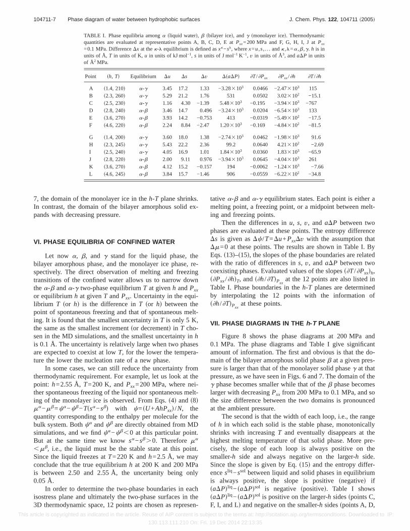
In order to determine the two-phase boundaries in eachisostress plane and ultimately the two-phase surfaces in the3D thermodynamic space, 12 points are chosen as represen-

tative a-b anda-g equilibrium states. Each point is either amelting point, a freezing point, or a midpoint between melt-ing and freezing points.

Then the differences inu, s, v, and aDP between twophases are evaluated at these points. The entropy differenceDs is given asDc /T=Du+PxxDv with the assumption thatDm=0 at these points. The results are shown in Table I. ByEqs.s13d–s15d, the slopes of the phase boundaries are relatedwith the ratio of differences ins, v, andaDP between twocoexisting phases. Evaluated values of the slopess]T/]Pxxdh,s]Pxx/]hdT, ands]h/]TdPxx

at the 12 points are also listed inTable I. Phase boundaries in theh-T planes are determinedby interpolating the 12 points with the information ofs]h/]TdPxx

at these points.

VII. PHASE DIAGRAMS IN THE h-T PLANE

Figure 8 shows the phase diagrams at 200 MPa and0.1 MPa. The phase diagrams and Table I give significantamount of information. The first and obvious is that the do-main of the bilayer amorphous solid phaseb at a given pres-sure is larger than that of the monolayer solid phaseg at thatpressure, as we have seen in Figs. 6 and 7. The domain of theg phase becomes smaller while that of theb phase becomeslarger with decreasingPxx from 200 MPa to 0.1 MPa, and sothe size difference between the two domains is pronouncedat the ambient pressure.

The second is that the width of each loop, i.e., the rangeof h in which each solid is the stable phase, monotonicallyshrinks with increasingT and eventually disappears at thehighest melting temperature of that solid phase. More pre-cisely, the slope of each loop is always positive on thesmaller-h side and always negative on the larger-h side.Since the slope is given by Eq.s15d and the entropy differ-encesliq −ssol between liquid and solid phases in equilibriumis always positive, the slope is positivesnegatived ifsaDPdliq −saDPdsol is negative spositived. Table I showssaDPdliq −saDPdsol is positive on the larger-h sidesspoints C,F, I, and Ld and negative on the smaller-h sidesspoints A, D,

TABLE I. Phase equilibria amonga sliquid waterd, b sbilayer iced, andg smonolayer iced. Thermodynamicquantities are evaluated at representative points A, B, C, D, E atPxx=200 MPa and F, G, H, I, J atPxx

=0.1 MPa. DifferenceDx at thek-l equilibrium is defined asxk−sl, wherex=u,s, . . . andk ,l=a ,b ,g. h is inunits of Å, T in units of K, u in units of kJ mol−1, s in units of J mol−1 K−1, v in units of Å3, andaDP in unitsof Å2 MPa.

Point sh, Td Equilibrium Du Ds Dv DsaDPd ]T/]Pxx ]Pxx/]h ]T/]h

A s1.4, 210d a-g 3.45 17.2 1.33 −3.283103 0.0466 −2.473103 115B s2.3, 260d a-g 5.29 21.2 1.76 531 0.0502 3.023102 −15.1C s2.5, 230d a-g 1.16 4.30 −1.39 5.483103 −0.195 −3.943103 −767D s2.8, 240d a-b 3.46 14.7 0.496 −3.243103 0.0204 −6.543103 133E s3.6, 270d a-b 3.93 14.2 −0.753 413 −0.0319 −5.493102 −17.5F s4.6, 220d a-b 2.24 8.84 −2.47 1.203103 −0.169 −4.843102 −81.5

G s1.4, 200d a-g 3.60 18.0 1.38 −2.743103 0.0462 −1.983103 91.6H s2.3, 245d a-g 5.43 22.2 2.36 99.2 0.0640 4.213102 −2.69I s2.5, 240d a-g 4.05 16.9 1.01 1.843103 0.0360 1.833103 −65.9J s2.8, 220d a-b 2.00 9.11 0.976 −3.943103 0.0645 −4.043103 261K s3.6, 270d a-b 4.12 15.2 −0.157 194 −0.0062 −1.243103 −7.66L s4.6, 245d a-b 3.84 15.7 −1.46 906 −0.0559 −6.223102 −34.8

104711-7 Phase diagram of water between hydrophobic surfaces J. Chem. Phys. 122, 104711 ~2005!

This article is copyrighted as indicated in the article. Reuse of AIP content is subject to the terms at: http://scitation.aip.org/termsconditions. Downloaded to IP:

130.113.111.210 On: Fri, 19 Dec 2014 22:13:35

G, and Jd. The same results would be expected for any quasi-two-dimensional system that exhibits liquid-solid phase tran-sitions under low or moderate lateral pressure. To see this, letfz be a normal force per molecule acting on the wall. IfPxx issmall compared toPzz in the liquid or solid phase, which isalways the case in our simulations,saDPdliq −saDPdsol. fz

liq

− fzsol. The phase change caused by decreasingh sso increas-

ing fzd should be in the direction that reduces the stress, i.e.,decreasesfz. Thus, fz

liq − fzsol.0 on the larger-h side of the

liquid-solid boundary whereasfzliq − fz

sol,0 on the smaller-hside. It is, therefore, generally expected for the system underlow or moderate lateral pressure that the slope]T/]h of asolid-liquid phase boundary is always positive on the small-h side and is always negative on the other side. It is nowclear that each loop is smooth everywhere including thepoint where the small-h and large-h phase boundaries meet atthe highest melting temperature.fThe shape of theb loophas been inferred from our earlier MD simulationsssee Fig.6b in Ref. 15d.g At the highest melting point, where]T/]h=0, saDPdliq =saDPdsol fEq. s15dg and in particularfz

liq = fzsol if

Pzz@ Pxx.The third is that the slope is much steeper on the inner

side of each loop where theb andg domains face each otherthan on the outer side of each loopsthe left side of thegdomain and the right side of theb domaind, which is againclearly shown in Fig. 8. The reason is less obvious and dif-fers in the two cases. Steepness of the slope is determined bythe magnitudes ofDs and DsaDPd. As to the b loop,uDsaDPdu is much larger on the inner side than on the outerside while Ds differs very little on both sidesscomparepoints D and F or J and L in Table Id, which is the reason ofthe steeper slope on the inner side. As to theg loop, on theother hand, the reason is thatDs is much smaller on the innerside than on the outer side whileuDsaDPdu is more or less thesame on both sidesscompare A and B in the tabled. Because

of their steep slopes, thea-b and a-g phase boundaries onthe inner sides do not meet in the temperature range above200 K, i.e., the temperature of thea-b-g triple point sat0.1 MPa and 200 MPad is lower than 200K. The reason thatthe system undergoes theb-g structural change above 200 Kat 0.1 and 200 MPa is that at such temperatures the meta-stable region of the bilayersmonolayerd solid phase extendsbeyond the region of the liquid phase to the region of themonolayersbilayerd solid phase.

Figure 9 shows the normal pressurePzz acting on thewalls as a function ofh at fixedT seither 260 or 240 Kd andfixed Pxx s0.1 MPad. At 260 K, the force curve exhibits apair of discontinuities, between which the system is in thebilayer ice phaseb and otherwise in the liquid phasea. Thenormal pressurePzz increases monotonically and rapidlywith decreasingh when the system is in the solid phasewhereas the curve ofPzz shows a local maximum and mini-mum reflecting layering structure of the liquid. Note that themagnitude ofPzz is much greater than that of fixedPxx, asmentioned above. Along the isothermal pass of 240 K, theforce curve exhibits another pair of discontinuities betweenwhich the system is in the monolayer ice phase, and now therange where the system is in the bilayer ice phase is widerthan at 260 K. These results are consistent with the phasediagram shown in Fig. 8sbd.

VIII. GLOBAL PHASE DIAGRAM

Table I and Fig. 8 suggest that pressure dependence ofthe solid-liquid phase equilibria is simple and small. Thus aglobal phase diagram, i.e., a three-dimensional diagram in

FIG. 8. Phase diagram of confined water:sad Pxx=200 MPa andsbd Pxx

=0.1 MPa. The symbolsa, b, andg indicate the liquid, bilayer solid, andmonolayer solid phases, respectively.

FIG. 9. Normal pressurePzz on the walls as a function ofh: sad 260 K andsbd 240 K. The lateral pressurePzz is fixed at 0.1 MPa.

104711-8 K. Koga and H. Tanaka J. Chem. Phys. 122, 104711 ~2005!

This article is copyrighted as indicated in the article. Reuse of AIP content is subject to the terms at: http://scitation.aip.org/termsconditions. Downloaded to IP:

130.113.111.210 On: Fri, 19 Dec 2014 22:13:35

the Pxx-h-T space, is obtained with reasonable accuracy bysimply interpolating phase diagrams at the two isostressplanessPxx=0.1 and 200 MPad, using derivatives of the equi-librium T or h with respect toPxx. The resulting surfaces ofthe phase boundaries are displayed in Fig. 10.

It is found that thea-b equilibrium T at h=4.6 Å de-creases with increasingPxx slike the melting curve of ice Ihd,whereas the equilibriumT at h=2.8 Å increases with in-creasingPxx slike the melting curve of most solidsd. This isbecause the confined water expands as it freezes into thebilayer solid on the large-h side of theb domain but itshrinks at the small-h side. Thea-g equilibrium T at h=2.5 Å initially increases with increasingPxx before reach-ing its maximum and then decreases, which reflects the pres-sure dependence of the volume change on the large-h side ofthe g domain. On the small-h sidesh=1.4 Åd, thea-g equi-

librium T monotonically increases with increasingPxx be-cause water shrinks as it freezes on that side.

The a-b equilibrium h at 200 K decreases monotoni-cally with increasingPxx on both the branches of the phaseboundary. This is becauseDv and DsaDPd have oppositesigns in any case. The dependence onPxx is noticeable on thelarge-h branch but it is practically undetectable on the small-h branch. Thea-g equilibrium h at 200 K is very weaklydependent onPxx on both branches of the boundary.

IX. CONCLUDING REMARKS

A phase diagram of water confined in a hydrophobic slitpore is obtained based on extensive MD simulations com-bined with the Clapeyron equations for the quasi-two-dimensional system. There are two solid phases, the mono-layer ice and the bilayer amorphoussor crystallined ice, aswell as a liquid phase in a small range of the effective widths0 Å,h,6 Åd above 200 K. The liquid-solid phase bound-aries of the two solids are convex curves with respect toh inthe isostressh-T planessFig. 8d and convex surfacessagainwith respect tohd in the three-dimensionalPxx-h-T spacesFig. 10d. It is explained based on a general argument whythe solid-liquid phase boundary on the large-h side of eachloop has always a negative slope and that on the small-h sidehas always a positive slope.

The monolayer ice has a smaller domain than the bilayersolid in a given isostress plane but the difference in domainsize becomes smaller as the lateral pressure is increased from0.1 to 200 MPa. The highest melting temperature is around260 and 270 K for the monolayer and bilayer solid, respec-tively, and the range ofh where each solid phase can bestable is of the order of subnanometer at lower temperatures.These conditions for the formation of monolayer and bilayersolids of water can well be achieved and controlled in thesurface force apparatus, atomic force microscopy, or othermodern experiments.

Structural analyses of the monolayer icesobtained fromthe TIP4P modeld show that there are four kinds of hydrogenbonds regularly arranged in the crystalfFig. 5scdg. The re-sidual entropy of the monolayer ice differs from that of the2D ice model and is exactly given by Eq.s18d, which issubextensive. No freezing transition is observed, i.e., liquidwater remains stable, in the range of 6 Å,h,20 Å at200 K and 0.1 MPa within the time scale of simulationsse.g., 30 nsd.

ACKNOWLEDGMENTS

The authors thank I. Hatano for providing his results onthe monolayer ice. This work was supported by Japan Soci-ety for the Promotion of Science and NAREGI.

1R. Evans and U. Marini Bettolo Marconi, J. Chem. Phys.86, 7138s1987d.2R. Evans, J. Phys.: Condens. Matter2, 8989s1990d.3L. D. Gelb, K. E. Gubbins, R. Radhakrishnan, and M. Sliwinska-Bartkowiak, Rep. Prog. Phys.62, 1573s1999d.

4C. Y. Lee, J. A. McCammon, and P. J. Rossky, J. Chem. Phys.80, 4448s1984d.

5S. H. Lee and P. J. Rossky, J. Chem. Phys.100, 3334s1994d.6J. Hautman, J. W. Halley, and Y.-J. Rhee, J. Chem. Phys.91, 467 s1989d.7M. Watanabe, A. M. Brodsky, and W. P. Reinhardt, J. Phys. Chem.95,

FIG. 10. Phase diagram of confined water in the three-dimensionalPxx-h-T space. Red and green curves are the phase boundaries of the monolayerice and those of the bilayersamorphousd ice, respectively. Thick curves arethe equilibriumT as a function ofh at givenPxx and thin curves are equi-librium T as a function ofPxx at givenh.

104711-9 Phase diagram of water between hydrophobic surfaces J. Chem. Phys. 122, 104711 ~2005!

This article is copyrighted as indicated in the article. Reuse of AIP content is subject to the terms at: http://scitation.aip.org/termsconditions. Downloaded to IP:

130.113.111.210 On: Fri, 19 Dec 2014 22:13:35

4593 s1991d.8A. Delville, J. Phys. Chem.97, 9703s1993d.9X. Xia and M. L. Berkowitz, Phys. Rev. Lett.74, 3193s1995d.

10J. C. Shelley and G. N. Patey, Mol. Phys.88, 385 s1996d.11K. Koga, X. C. Zeng, and H. Tanaka, Chem. Phys. Lett.285, 278s1998d.12M. Meyer and H. E. Stanley, J. Phys. Chem. B103, 9728s1999d.13K. Koga, X. C. Zeng, and H. Tanaka, Phys. Rev. Lett.79, 5262s1997d.14K. Koga, H. Tanaka, and X. C. Zeng, NaturesLondond 408, 564 s2000d.15K. Koga, J. Chem. Phys.116, 10882s2002d.16R. Zangi and A. E. Mark, Phys. Rev. Lett.91, 025502s2003d.17K. Koga, G. T. Gao, H. Tanaka, and X. C. Zeng, NaturesLondond 412,

802 s2001d.

18K. Koga, G. T. Gao, H. Tanaka, and X. C. Zeng, Physica A314, 462s2002d.

19Y. Maniwa, H. Kataura, M. Abe, S. Suzuki, Y. Achiba, H. Kira, and K.Matsuda, J. Phys. Soc. Jpn.71, 2863s2002d.

20W. L. Jorgensen, J. Chandrasekhar, J. D. Madura, R. W. Impey, and M. L.Klein, J. Chem. Phys.79, 926 s1983d.

21I. Ohimine, H. Tanaka, and P. Wolynes, J. Chem. Phys.89, 5852s1988d.

22W. A. Steele, Surf. Sci.36, 317 s1973d.23S. Nosé, J. Chem. Phys.81, 511 s1984d.24J. Bai, X. C. Zeng, K. Koga, and H. Tanaka, Mol. Sim.29, 619 s2003d.25E. H. Lieb, Phys. Rev. Lett.18, 692 s1967d.

104711-10 K. Koga and H. Tanaka J. Chem. Phys. 122, 104711 ~2005!

This article is copyrighted as indicated in the article. Reuse of AIP content is subject to the terms at: http://scitation.aip.org/termsconditions. Downloaded to IP:

130.113.111.210 On: Fri, 19 Dec 2014 22:13:35