www.iap.uni-jena.de
Optical Design with Zemax
for PhD - Advanced
Lecture 16: Physical modelling I
2019-02-27
Herbert Gross
Speaker: Uwe Lippmann
Winter term 2018/19
2
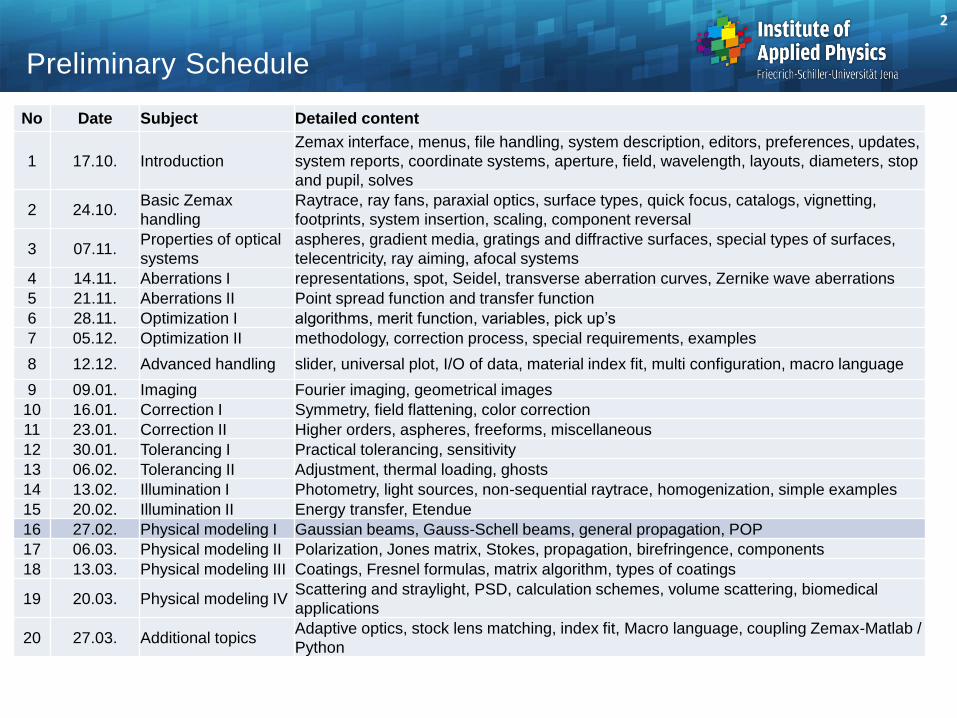
Preliminary Schedule
No Date Subject Detailed content
1 17.10. Introduction
Zemax interface, menus, file handling, system description, editors, preferences, updates,
system reports, coordinate systems, aperture, field, wavelength, layouts, diameters, stop
and pupil, solves
2 24.10.Basic Zemax
handling
Raytrace, ray fans, paraxial optics, surface types, quick focus, catalogs, vignetting,
footprints, system insertion, scaling, component reversal
3 07.11.Properties of optical
systems
aspheres, gradient media, gratings and diffractive surfaces, special types of surfaces,
telecentricity, ray aiming, afocal systems
4 14.11. Aberrations I representations, spot, Seidel, transverse aberration curves, Zernike wave aberrations
5 21.11. Aberrations II Point spread function and transfer function
6 28.11. Optimization I algorithms, merit function, variables, pick up’s
7 05.12. Optimization II methodology, correction process, special requirements, examples
8 12.12. Advanced handling slider, universal plot, I/O of data, material index fit, multi configuration, macro language
9 09.01. Imaging Fourier imaging, geometrical images
10 16.01. Correction I Symmetry, field flattening, color correction
11 23.01. Correction II Higher orders, aspheres, freeforms, miscellaneous
12 30.01. Tolerancing I Practical tolerancing, sensitivity
13 06.02. Tolerancing II Adjustment, thermal loading, ghosts
14 13.02. Illumination I Photometry, light sources, non-sequential raytrace, homogenization, simple examples
15 20.02. Illumination II Energy transfer, Etendue
16 27.02. Physical modeling I Gaussian beams, Gauss-Schell beams, general propagation, POP
17 06.03. Physical modeling II Polarization, Jones matrix, Stokes, propagation, birefringence, components
18 13.03. Physical modeling III Coatings, Fresnel formulas, matrix algorithm, types of coatings
19 20.03. Physical modeling IVScattering and straylight, PSD, calculation schemes, volume scattering, biomedical
applications
20 27.03. Additional topicsAdaptive optics, stock lens matching, index fit, Macro language, coupling Zemax-Matlab /
Python

Content
Gaussian beams
Gauss-Schell beams
Non-fundamental modes
Propagation methods
Numerical issues
POP in Zemax

2
2
)(
w
r
oeIrI
Gaussian Beams, Transverse Beam Profile
I(r) / I0
r / w
0.3
0.4
0.5
0.6
0.7
0.8
0.9
1
-2 -1 0 1 2
0.135
0.0111.5
0.589
1.0
Transverse beam profile is gaussian
Beam radius w at 13.5% intensity

Expansion of the intensity distribution around the waist I(r,z)
Gaussian Beams
z
asymptotic
lines
x
hyperbolic
caustic curve
wo
w(z)
R(z)
o
zo

-4 -3 -2 -1 1 2 3 4
-4
-3
-2
-1
1
2
3
4
z / z
r / w
o
o
asymptotic
far field
waist
w(z)
o
intensity
13.5 %
Geometry of Gaussian Beams

2
2
2
1
2
2
2 1
2),(
o
To
z
zzw
r
o
To
e
z
zzw
PzrI
2
0 1)(
o
T
z
zzwzw
00000
zzw
o
o
Gaussian Beams, Definitions and Parameter
Paraxial TEM00 fundamental mode
Transverse intensity is gaussian
Axial isophotes are hyperbolic
Beam radius at 13.5% intensity
Only 2 independent beam parameters of the set:
1. waist radius wo
2. far field divergence angle o
3. Rayleigh range zo
4. Wavelength o
Relations
f
zfz
zzz
TT
oTT
1
1
1112'
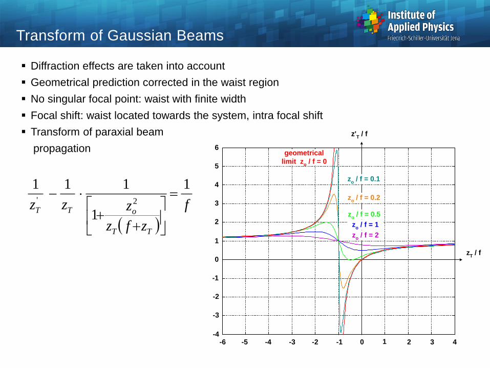
Transform of Gaussian Beams
Diffraction effects are taken into account
Geometrical prediction corrected in the waist region
No singular focal point: waist with finite width
Focal shift: waist located towards the system, intra focal shift
Transform of paraxial beam
propagation
z'T / f
zT / f
-6 -5 -4 -3 -2 -1 0 1 2 3 4-4
-3
-2
-1
0
1
2
3
4
5
6
zo / f = 0.1
zo / f = 0.2
zo / f = 0.5
zo / f = 1
zo / f = 2
geometrical
limit zo / f = 0
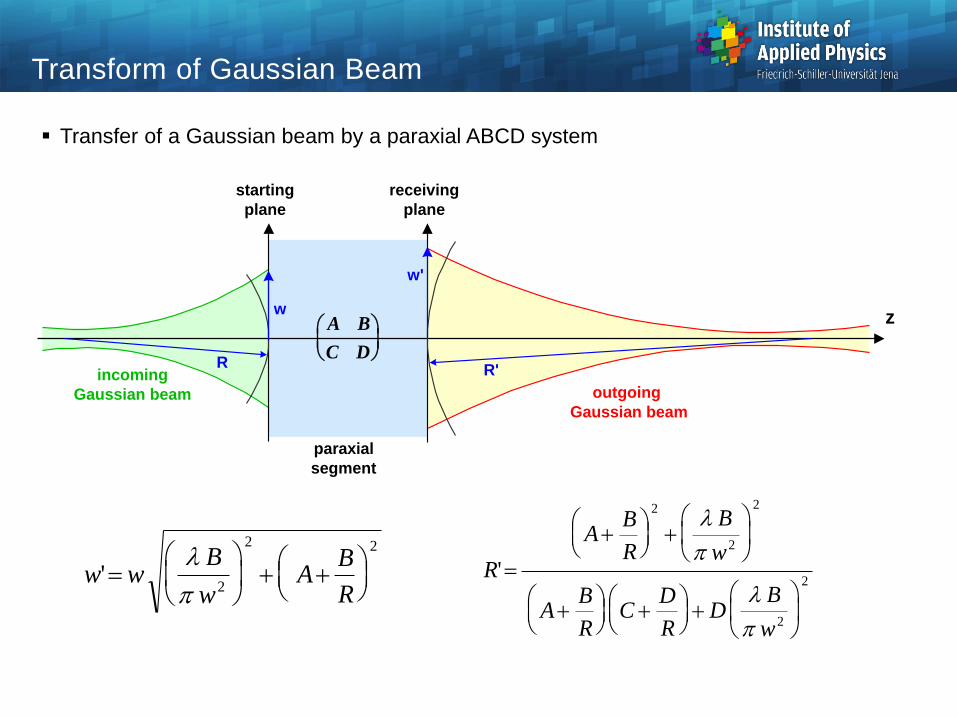
Transform of Gaussian Beam
R
w
w'
R'
starting
plane
receiving
plane
paraxial
segment
A B
C D
incoming
Gaussian beam
z
outgoing
Gaussian beam
Transfer of a Gaussian beam by a paraxial ABCD system
w wB
wA
B
R'
2
2 2
R
AB
R
B
w
AB
RC
D
RD
B
w
'
2
2
2
2
2
-2
0
2-8
-6
-4
-2
0
2
4
6
8
0
0.5
1
z
intensity I
[a.u.]
x
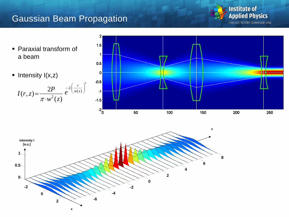
Gaussian Beam Propagation
Paraxial transform of
a beam
Intensity I(x,z)2
)(2
2 )(
2),(
zw
r
ezw
PzrI

2
21
2
1
21 )0,(
cL
rr
ezrr
2
1
2
1
c
o
L
w
2
2 11
c
o
L
wM
Gauß-Schell Beam: Definition
Partial coherent beams:
1. intensity profile gaussian
2. Coherence function gaussian
Extension of gaussian beams with similar description
Additional parameter: lateral coherence length Lc
Normalized degree of coherence
Beam quality depends on coherence
Approximate model do characterize multimode beams
-4 -3 -2 -1 0 1 2 3 4
1
2
3
4
0 z / zo
w / wo
0.25
0.50
1.0
-4 -3 -2 -1 0 1 2 3 4
1
2
3
4
0 z / zo
w / wo
1.0
0.50 0.25
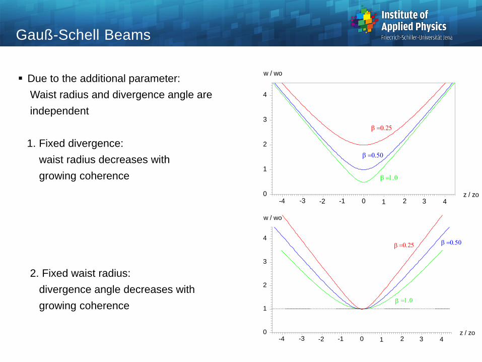
Gauß-Schell Beams
Due to the additional parameter:
Waist radius and divergence angle are
independent
1. Fixed divergence:
waist radius decreases with
growing coherence
2. Fixed waist radius:
divergence angle decreases with
growing coherence
f
zfz
zzz
TT
oTT
1
1
1112'
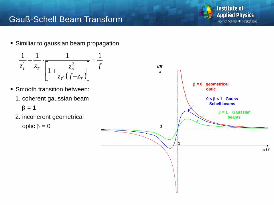
s'/f'
1
1
s / f
= 0 geometrical
optic
0 < < 1 Gauss-
Schell beams
= 1 Gaussian
beams
Gauß-Schell Beam Transform
Similiar to gaussian beam propagation
Smooth transition between:
1. coherent gaussian beam
= 1
2. incoherent geometrical
optic = 0

Hermite Gaussian Modes
n = 0 n = 1 n = 2 n = 3 n = 4 n = 5
m = 5
m = 4
m = 3
m = 2
m = 1
m = 0
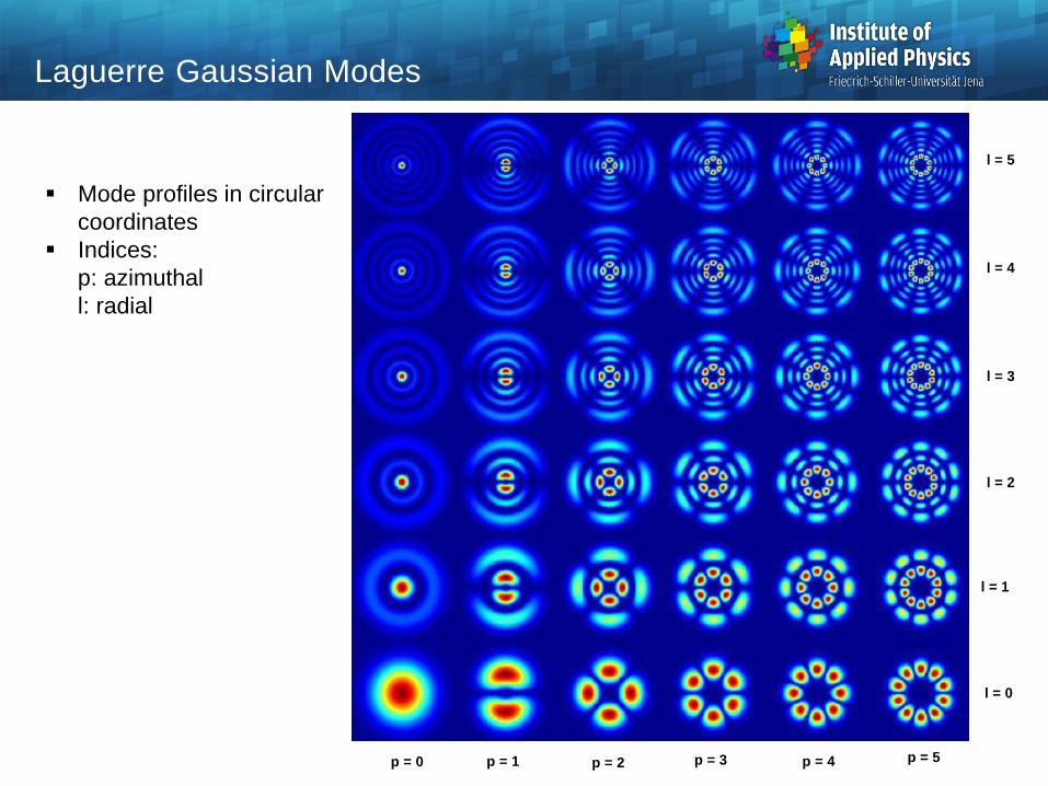
Mode profiles in circular
coordinates
Indices:
p: azimuthal
l: radial
p = 5p = 4p = 3p = 2
l = 5
p = 0 p = 1
l = 0
l = 1
l = 2
l = 3
l = 4
Laguerre Gaussian Modes

Keplerian telescope with pinhole in focal plane
Higher modes with larger spatial extend are blocked:
only fundamental mode transmitted, beam clean up, mode filter
Approximate size of pinhole diameter: 20.637Pinhole
in in
f fD
w w
Beam Clean Up Filter
z
win
f
second lens ffirst lens f stop d
f wo
a/wo = 1
0 1 2 3 4 5 610
-12
10-10
10-8
10-6
10-4
10-2
100
a/wo = 2
a/wo = 3
a/wo = 4
x
Log |A|
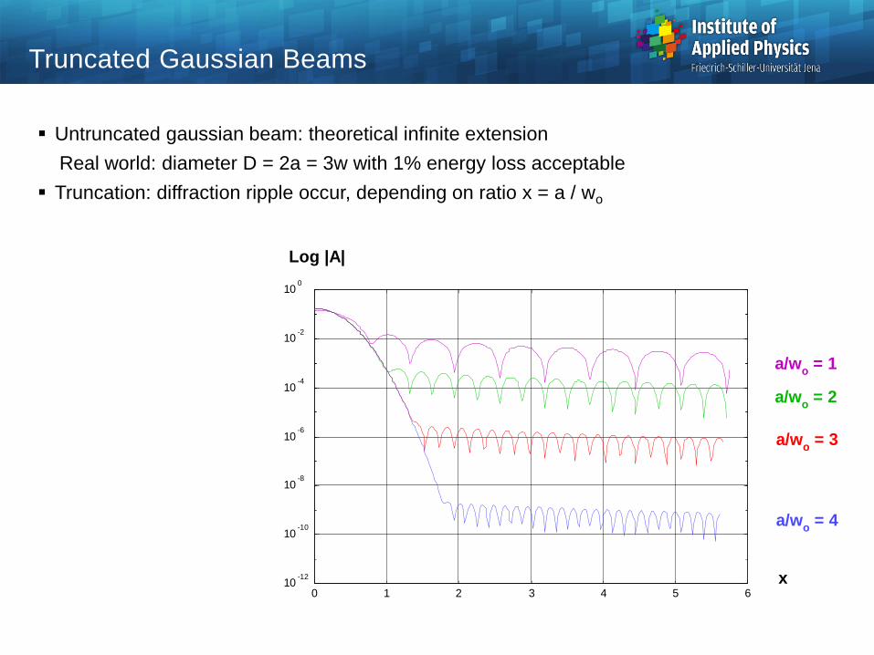
Truncated Gaussian Beams
Untruncated gaussian beam: theoretical infinite extension
Real world: diameter D = 2a = 3w with 1% energy loss acceptable
Truncation: diffraction ripple occur, depending on ratio x = a / wo

Focussed Gaussian beam with spherical aberration
Asymmetry intra - extra focal
depending on sign of spherical aberration
Gaussian profile perturbed
Gaussian Beam with Spherical Aberration
c9 = -0.25
c9 = 0.25
c9 = 0

Solution Methods of the Maxwell Equations
Maxwell-
equations
diffraction
integrals
asymptotic
approximation
Fresnel
approximation
Fraunhofer
approximation
finite
elements
finite
differences
exact/
numerical1st
approximation
direct
solutions of
the PDE
spectral
methods
plane wave
spectrum
vector
potentials
2nd
approximation
finite element
method
boundary
element
method
hybrid method
BEM + FEM
Debye
approximation
Kirchhoff-
integral
Rayleigh-
Sommerfeld
1st kind
Rayleigh-
Sommerfeld
2nd kind
mode
expansion
boundary
edge wave
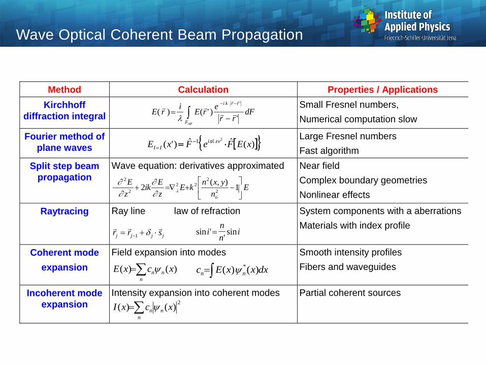
Method Calculation Properties / Applications
Kirchhoff
diffraction integral E r
iE r
e
r rdF
i k r r
FAP
( ) ( ' )'
'
Small Fresnel numbers,
Numerical computation slow
Fourier method of
plane waves )(ˆˆ)'(21 xEFeFxE zvi
II
Large Fresnel numbers
Fast algorithm
Split step beam
propagation
Wave equation: derivatives approximated
En
yxnkE
z
Eik
z
E
o
1
),(2
2
222
2
2
Near field
Complex boundary geometries
Nonlinear effects
Raytracing Ray line law of refraction
r r sj j j j 1 sin '
'sini
n
ni
System components with a aberrations
Materials with index profile
Coherent mode
expansion
Field expansion into modes
n
nn xcxE )()( dxxxEc nn )()( *
Smooth intensity profiles
Fibers and waveguides
Incoherent mode
expansion
Intensity expansion into coherent modes
n
nn xcxI2
)()(
Partial coherent sources
Wave Optical Coherent Beam Propagation
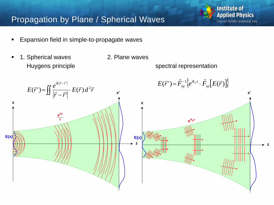
Propagation by Plane / Spherical Waves
Expansion field in simple-to-propagate waves
1. Spherical waves 2. Plane waves
Huygens principle spectral representation
rdrErr
erE
rrik
2
'
)('
)'(
x
x'
z
E(x)
eikr
r
)(ˆˆ)'( 1 rEFeFrE xy
zik
xyz
x
x'
z
E(x)
eik z z

Kirchhoff diffraction integral in Fresnel approximation
Fourier transform: plan wave expansion
Equivalent form
Curvature removed
Calculation in spherical coordinates
Fresnel Propagation with Equivalence Transform
222 )1(
1'
)1(
)(ˆˆ)'(x
z
Miv
M
zix
Mz
MiM
zik
OO exEFeFeM
exE
x
R<0
z1
z2
starting
plane
observation
plane 1
focus
observation
plane 2
R'<0
R2'>0
x''
x x'
a
a
xxz
i
dxexECxE
2'
)()'(

Optimal Conditioning of the Fresnel-Propagator
Four different cases of propagation in a caustic
Starting plane / final plane inside/outside the focal region
Flattening transform only necessary outside focal range
z
y
inside waist region:
weak curvature
outside waist region:
strong curvature
case 1 : I - I
case 42 : O - O
case 41 : O - O
case 2 : O - I case 3 : I - O
waist
plane
R < 0
R > 0
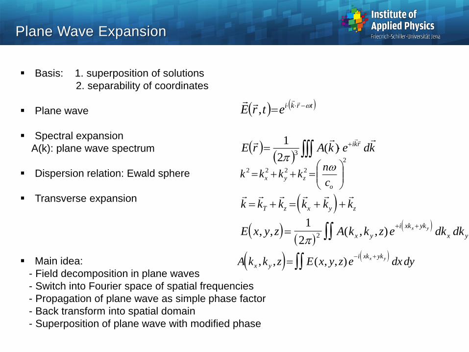
Basis: 1. superposition of solutions
2. separability of coordinates
Plane wave
Spectral expansion
A(k): plane wave spectrum
Dispersion relation: Ewald sphere
Transverse expansion
Main idea:
- Field decomposition in plane waves
- Switch into Fourier space of spatial frequencies
- Propagation of plane wave as simple phase factor
- Back transform into spatial domain
- Superposition of plane wave with modified phase
Plane Wave Expansion
kdekArE rki
)(
2
13
trkietrE
,
2
2222
o
zyxc
nkkkk
E x y z A k k z e dk dkx y
i xk yk
x y
x y, , ( , , )
1
22
k k k k k kT z x y z
A k k z E x y z e dxdyx y
i xk ykx y, , ( , , )

Propagation of plane waves:
pure phase factor
1. exact sphere
2. Fresnel quadratic approximation
Evanescent waves
components damped in z
important only for near field setups
Propagation algorithm
x-y-sections are coupled
Paraxial approximation
x-y-section decoupled
Plane Wave Expansion
22
22
0,,
0,,,, 2
yx
yx
vvzizik
yx
kkk
iz
zik
yxyx
eevvA
eekkAzkkA
evanescentkkforkkkik yxyxz ,0222
0
22
),(ˆˆ
),(ˆˆ)','(
222/121
1
yxEFeF
yxEFeFyxE
xy
vviz
xy
xy
zik
xy
yx
z
),(ˆˆ)','(22
1 yxEFeFyxE xy
vvzi
xyyx
𝐴 𝑘𝑥 , 𝑘𝑦 , 𝑧 = 𝐴 𝑘𝑥 , 𝑘𝑦 , 0 𝑒−𝑖𝑘𝑧𝑧 = 𝐴 𝑘𝑥 , 𝑘𝑦 , 0 𝑒−𝑖𝑘𝑧 1−
𝑘𝑥𝑘
2
−𝑘𝑦𝑘
2
a
NAaRRD
pxN
RRvx
'
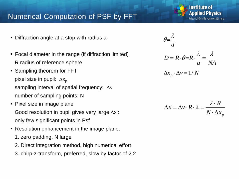
Numerical Computation of PSF by FFT
Diffraction angle at a stop with radius a
Focal diameter in the range (if diffraction limited)
R radius of reference sphere
Sampling theorem for FFT
pixel size in pupil: xp
sampling interval of spatial frequency: n
number of sampling points: N
Pixel size in image plane
Good resolution in pupil gives very large x‘:
only few significant points in Psf
Resolution enhancement in the image plane:
1. zero padding, N large
2. Direct integration method, high numerical effort
3. chirp-z-transform, preferred, slow by factor of 2.2
Nvxp /1
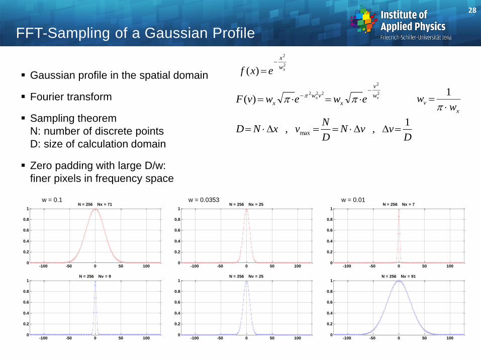
Gaussian profile in the spatial domain
Fourier transform
Sampling theorem
N: number of discrete points
D: size of calculation domain
Zero padding with large D/w:
finer pixels in frequency space
28
FFT-Sampling of a Gaussian Profile
2
2
)( xw
x
exf
2
2
222
)( vx w
v
x
vw
x ewewvF
DvvN
D
NvxND
1,, max
x
vw
w
1
-100 -50 0 50 1000
0.2
0.4
0.6
0.8
1N = 256 Nx = 25
-100 -50 0 50 1000
0.2
0.4
0.6
0.8
1N = 256 Nv = 25
w = 0.1 w = 0.0353
-100 -50 0 50 1000
0.2
0.4
0.6
0.8
1N = 256 Nx = 71
-100 -50 0 50 1000
0.2
0.4
0.6
0.8
1N = 256 Nv = 9
w = 0.01
-100 -50 0 50 1000
0.2
0.4
0.6
0.8
1N = 256 Nx = 7
-100 -50 0 50 1000
0.2
0.4
0.6
0.8
1N = 256 Nv = 91
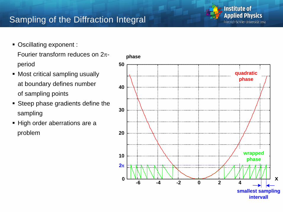
Sampling of the Diffraction Integral
x-6 -4 -2 0 2 4
0
10
20
30
40
50
quadratic
phase
wrapped
phase
2
smallest sampling
intervall
phase
Oscillating exponent :
Fourier transform reduces on 2-
period
Most critical sampling usually
at boundary defines number
of sampling points
Steep phase gradients define the
sampling
High order aberrations are a
problem
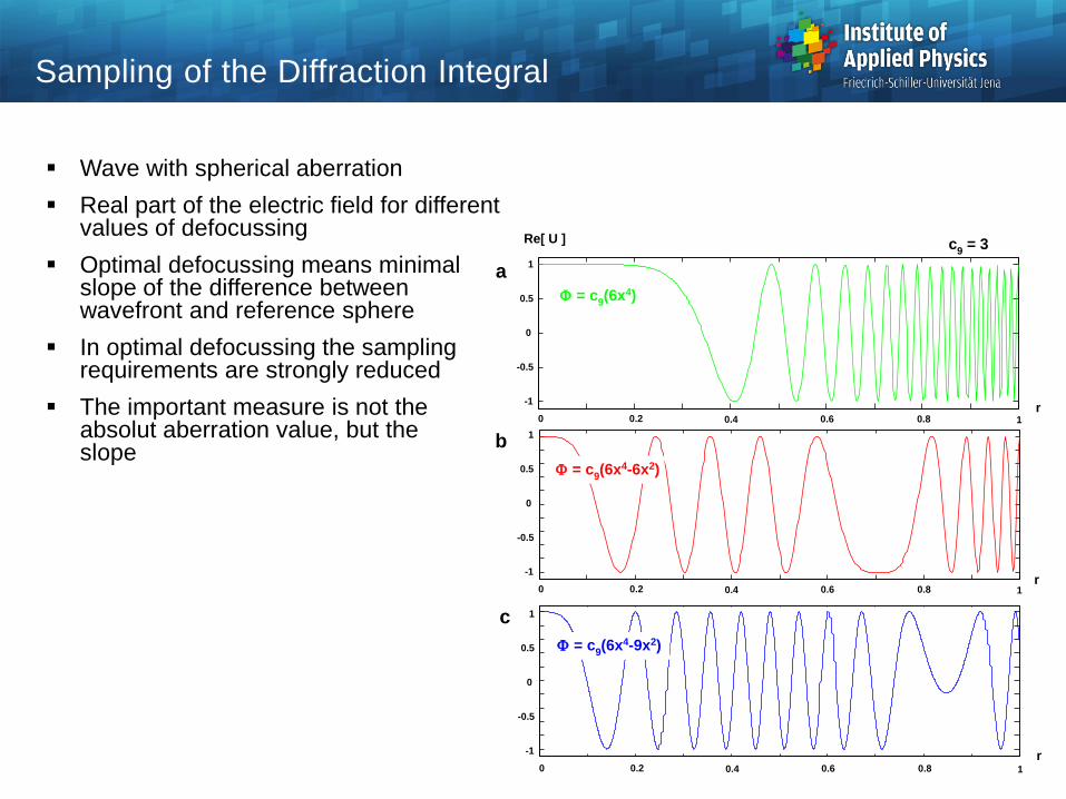
Sampling of the Diffraction Integral
c9 = 3
0 0.2 0.4 0.6 0.8 1
-1
-0.5
0
0.5
1
0 0.2 0.4 0.6 0.8 1
-1
-0.5
0
0.5
1
= c9(6x4-6x2)
r
r
Re[ U ]
= c9(6x4)
0 0.2 0.4 0.6 0.8 1
-1
-0.5
0
0.5
1
r
= c9(6x4-9x2)
a
b
c
Wave with spherical aberration
Real part of the electric field for differentvalues of defocussing
Optimal defocussing means minimalslope of the difference betweenwavefront and reference sphere
In optimal defocussing the samplingrequirements are strongly reduced
The important measure is not theabsolut aberration value, but the slope
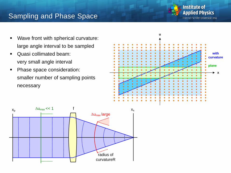
Sampling and Phase Space
x
u
with
curvature
plane
f
radius of
curvatureR
xp xsumax << 1
umax large
Wave front with spherical curvature:
large angle interval to be sampled
Quasi collimated beam:
very small angle interval
Phase space consideration:
smaller number of sampling points
necessary

Setting of initial beam and
sampling parameters
Beam Propagation in Zemax
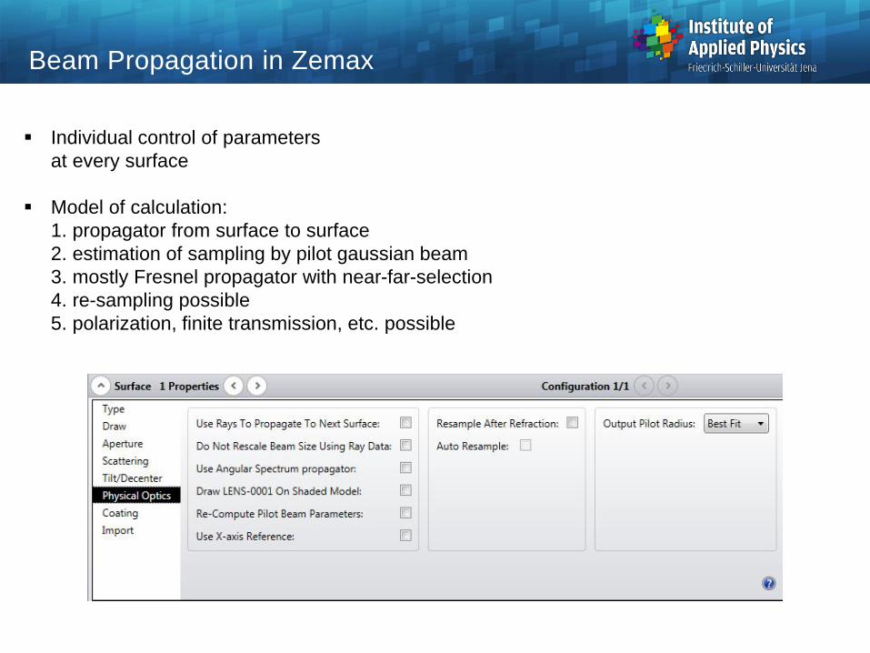
Individual control of parameters
at every surface
Model of calculation:
1. propagator from surface to surface
2. estimation of sampling by pilot gaussian beam
3. mostly Fresnel propagator with near-far-selection
4. re-sampling possible
5. polarization, finite transmission, etc. possible
Beam Propagation in Zemax
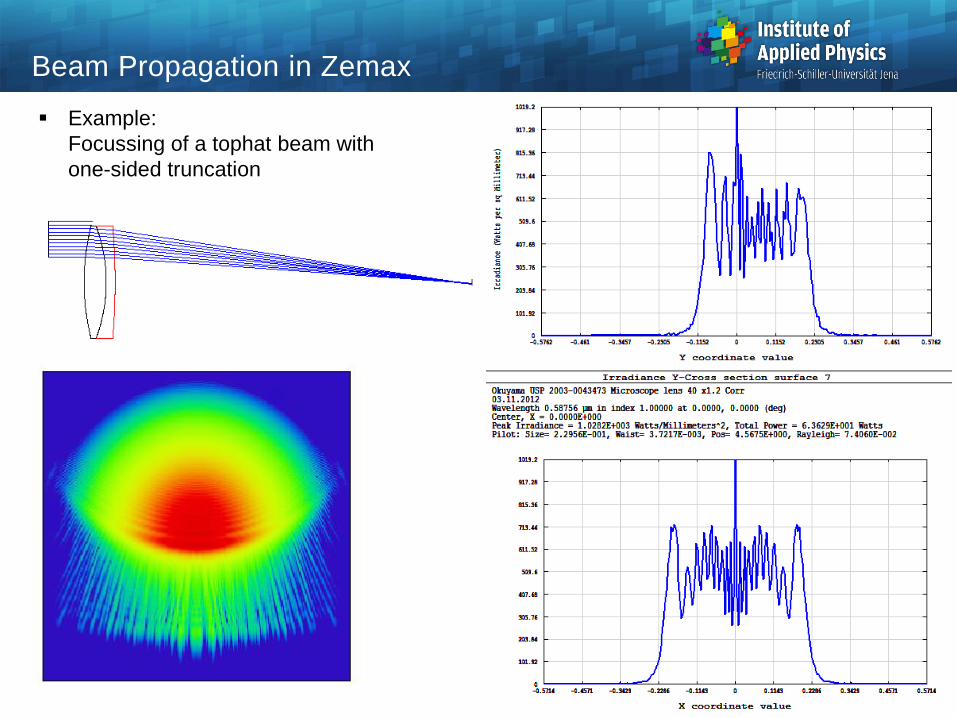
Example:
Focussing of a tophat beam with
one-sided truncation
Beam Propagation in Zemax

1. Geometrical with raytrace:
image of circular object
only geometrical truncation on the dia-
meter is considered
2. Geometrical with raytrace:
footprint
only geometrical truncation on the dia-
meter is considered
3. Monomode fiber:
special menu entry:
Calculations / Fiber Coupling Efficiency
Transmission, apodization, vignetting
are taken into account
Angle and spatial acceptance is
considered simultaneously
Huygens integral PSF is calculated
4. With physical optical propagation
Most general tool
35
Fiber Coupling

Monomode fiber coupling example
36
Fiber Coupling
Recommended