www.iap.uni-jena.de

Optical Design with Zemax

for PhD

Lecture 12: Physical Optics

2016-03-23

Herbert Gross

Winter term 2015

2

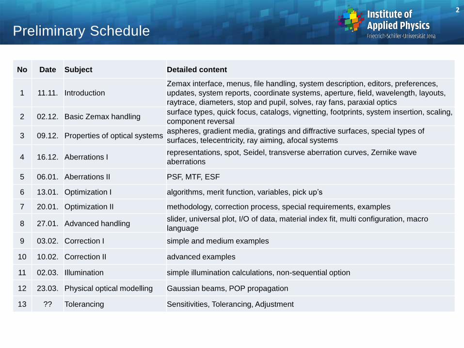
Preliminary Schedule

No Date Subject Detailed content

1 11.11. Introduction

Zemax interface, menus, file handling, system description, editors, preferences,

updates, system reports, coordinate systems, aperture, field, wavelength, layouts,

raytrace, diameters, stop and pupil, solves, ray fans, paraxial optics

2 02.12. Basic Zemax handling surface types, quick focus, catalogs, vignetting, footprints, system insertion, scaling,

component reversal

3 09.12. Properties of optical systems aspheres, gradient media, gratings and diffractive surfaces, special types of

surfaces, telecentricity, ray aiming, afocal systems

4 16.12. Aberrations I representations, spot, Seidel, transverse aberration curves, Zernike wave

aberrations

5 06.01. Aberrations II PSF, MTF, ESF

6 13.01. Optimization I algorithms, merit function, variables, pick up’s

7 20.01. Optimization II methodology, correction process, special requirements, examples

8 27.01. Advanced handling slider, universal plot, I/O of data, material index fit, multi configuration, macro

language

9 03.02. Correction I simple and medium examples

10 10.02. Correction II advanced examples

11 02.03. Illumination simple illumination calculations, non-sequential option

12 23.03. Physical optical modelling Gaussian beams, POP propagation

13 ?? Tolerancing Sensitivities, Tolerancing, Adjustment

Content

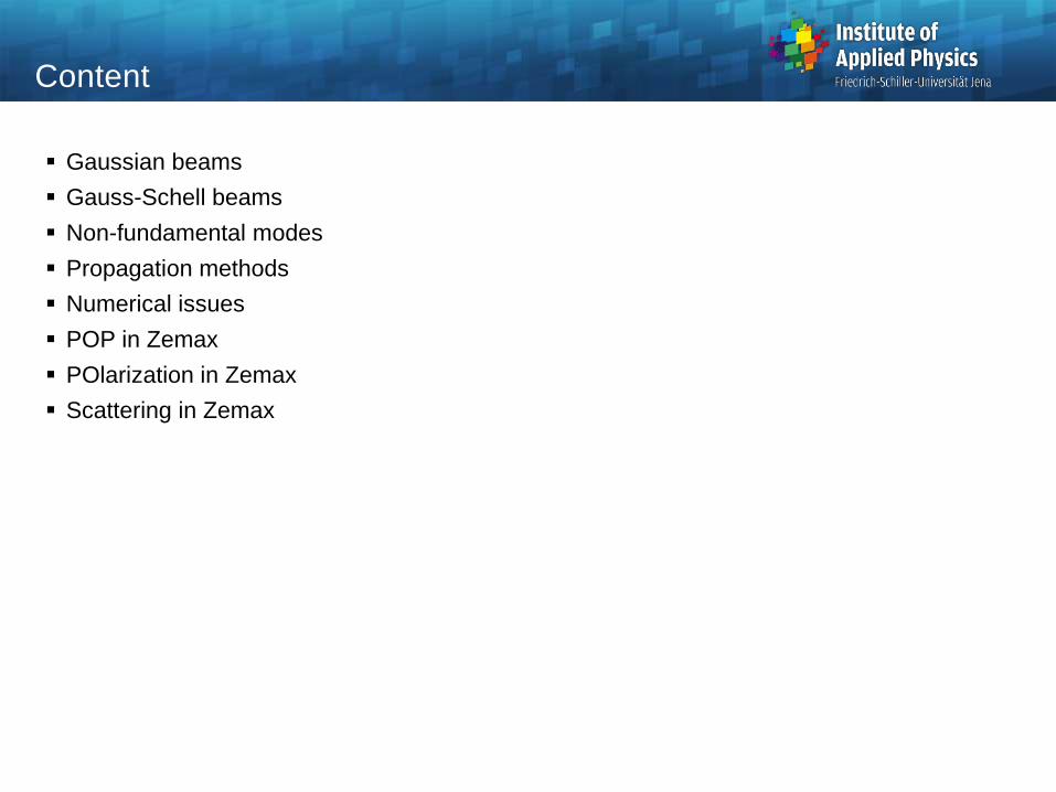
Gaussian beams

Gauss-Schell beams

Non-fundamental modes

Propagation methods

Numerical issues

POP in Zemax

POlarization in Zemax

Scattering in Zemax

2

2

)(

w

r

oeIrI

Gaussian Beams, Transverse Beam Profile

I(r) / I0

r / w

0.3

0.4

0.5

0.6

0.7

0.8

0.9

1

-2 -1 0 1 2

0.135

0.0111.5

0.589

1.0

Transverse beam profile is gaussian

Beam radius w at 13.5% intensity

Expansion of the intensity distribution around the waist I(r,z)

Gaussian Beams

z

asymptotic

lines

x

hyperbolic

caustic curve

wo

w(z)

R(z)

o

zo

-4 -3 -2 -1 1 2 3 4

-4

-3

-2

-1

1

2

3

4

z / z

r / w

o

o

asymptotic

far field

waist

w(z)

o

intensity

13.5 %

Geometry of Gaussian Beams

2

2

2

1

2

2

2 1

2),(

o

To

z

zzw

r

o

To

e

z

zzw

PzrI

2

0 1)(

o

T

z

zzwzw

00000

zzw

o

o

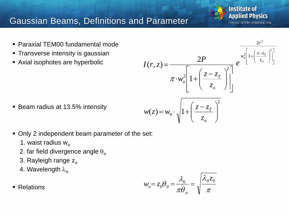
Gaussian Beams, Definitions and Parameter

Paraxial TEM00 fundamental mode

Transverse intensity is gaussian

Axial isophotes are hyperbolic

Beam radius at 13.5% intensity

Only 2 independent beam parameter of the set:

1. waist radius wo

2. far field divergence angle o

3. Rayleigh range zo

4. Wavelength o

Relations

f

zfz

zzz

TT

oTT

1

1

1112'

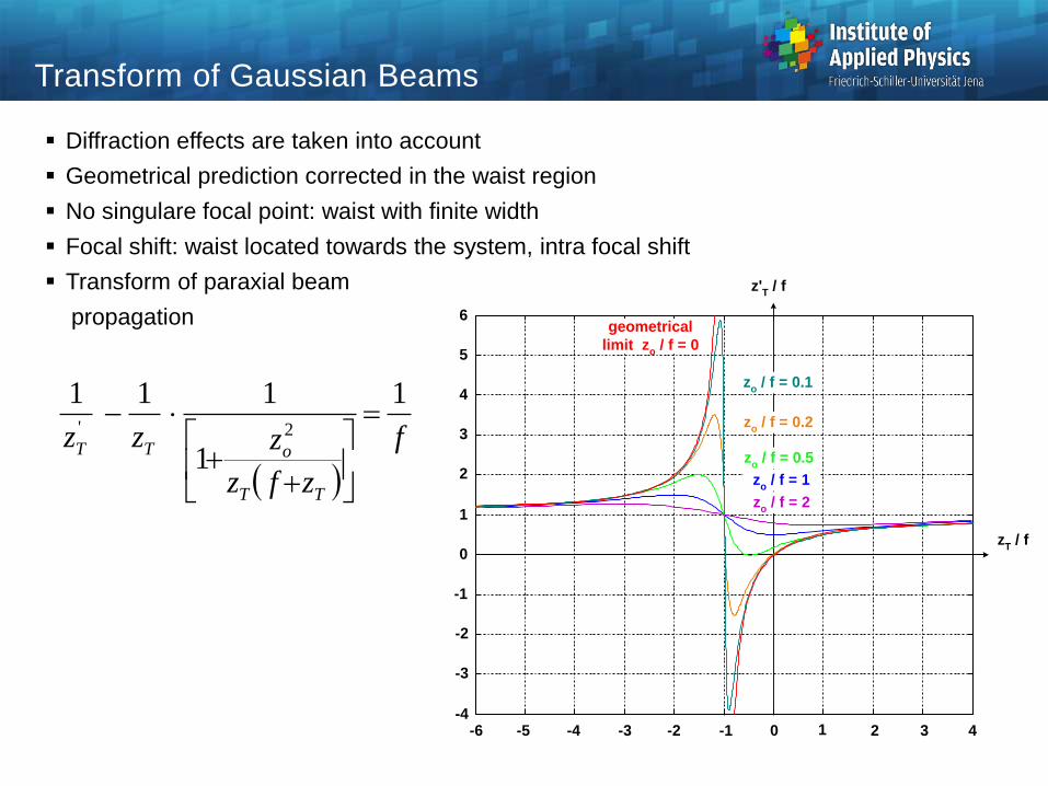
Transform of Gaussian Beams

Diffraction effects are taken into account

Geometrical prediction corrected in the waist region

No singulare focal point: waist with finite width

Focal shift: waist located towards the system, intra focal shift

Transform of paraxial beam

propagation

z'T / f

zT / f

-6 -5 -4 -3 -2 -1 0 1 2 3 4-4

-3

-2

-1

0

1

2

3

4

5

6

zo / f = 0.1

zo / f = 0.2

zo / f = 0.5

zo / f = 1

zo / f = 2

geometrical

limit zo / f = 0

Transform of Gaussian Beam

R

w

w'

R'

starting

plane

receiving

plane

paraxial

segment

A B

C D

incoming

Gaussian beam

z

outgoing

Gaussian beam

Transfer of a Gaussian beam by a paraxial ABCD system

w wB

wA

B

R'

2

2 2

R

AB

R

B

w

AB

RC

D

RD

B

w

'

2

2

2

2

2

-2

0

2-8

-6

-4

-2

0

2

4

6

8

0

0.5

1

z

intensity I

[a.u.]

x

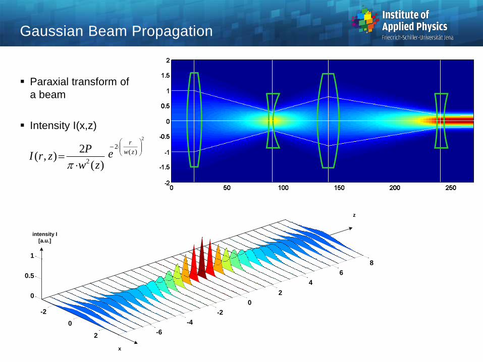
Gaussian Beam Propagation

Paraxial transform of

a beam

Intensity I(x,z)

2

)(2

2 )(

2),(

zw

r

ezw

PzrI

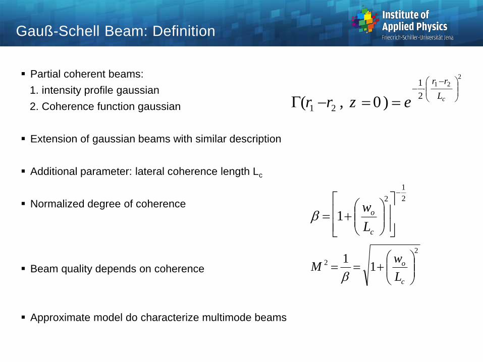
2

21

2

1

21 )0,(

cL

rr

ezrr

2

1

2

1

c

o

L

w

2

2 11

c

o

L

wM

Gauß-Schell Beam: Definition

Partial coherent beams:

1. intensity profile gaussian

2. Coherence function gaussian

Extension of gaussian beams with similar description

Additional parameter: lateral coherence length Lc

Normalized degree of coherence

Beam quality depends on coherence

Approximate model do characterize multimode beams

-4 -3 -2 -1 0 1 2 3 4

1

2

3

4

0 z / zo

w / wo

0.25

0.50

1.0

-4 -3 -2 -1 0 1 2 3 4

1

2

3

4

0 z / zo

w / wo

1.0

0.50 0.25

Gauß-Schell Beams

Due to the additional parameter:

Waist radius and divergence angle are

independent

1. Fixed divergence:

waist radius decreases with

growing coherence

2. Fixed waist radius:

divergence angle decreases with

growing coherence

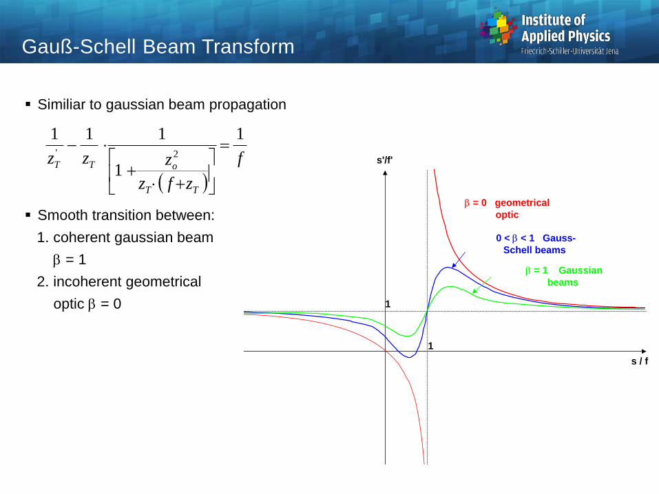
f

zfz

zzz

TT

oTT

1

1

1112'

s'/f'

1

1

s / f

= 0 geometrical

optic

0 < < 1 Gauss-

Schell beams

= 1 Gaussian

beams

Gauß-Schell Beam Transform

Similiar to gaussian beam propagation

Smooth transition between:

1. coherent gaussian beam

= 1

2. incoherent geometrical

optic = 0

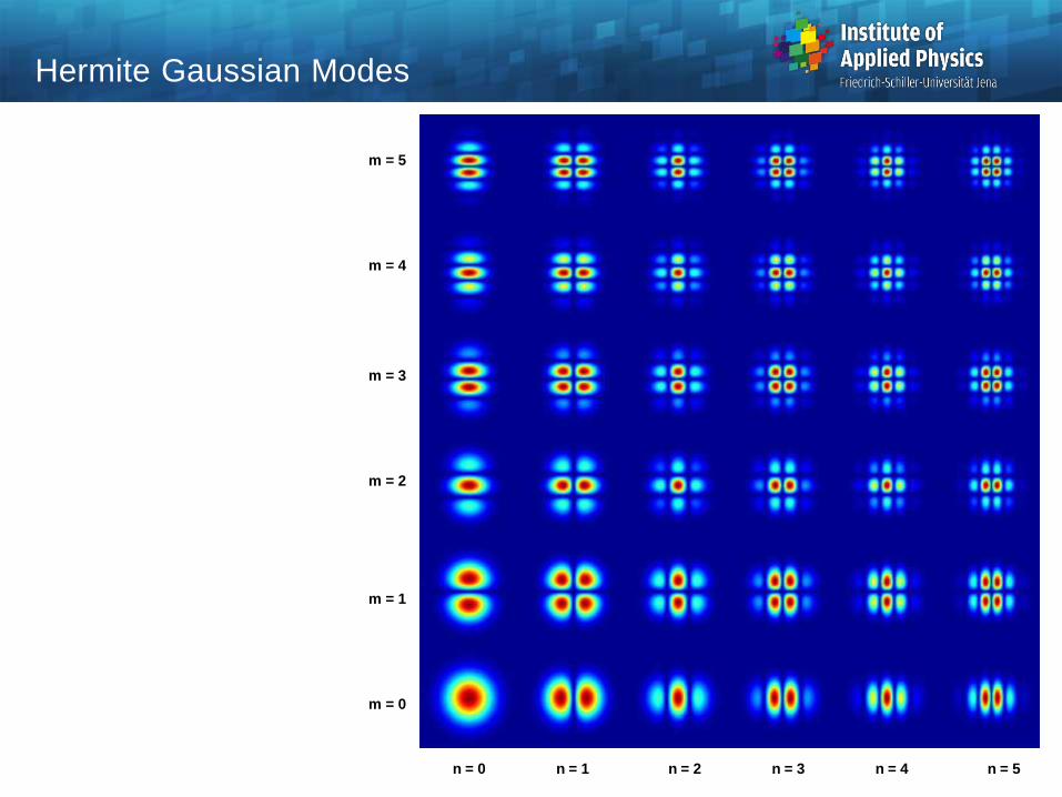
Hermite Gaussian Modes

n = 0 n = 1 n = 2 n = 3 n = 4 n = 5

m = 5

m = 4

m = 3

m = 2

m = 1

m = 0

a/wo = 1

0 1 2 3 4 5 610

-12

10-10

10-8

10-6

10-4

10-2

100

a/wo = 2

a/wo = 3

a/wo = 4

x

Log |A|

Truncated Gaussian Beams

Untruncated gaussian beam: theoretical infinite extension

Real world: diameter D = 2a = 3w with 1% energy loss acceptable

Truncation: diffraction ripple occur, depending on ratio x = a / wo

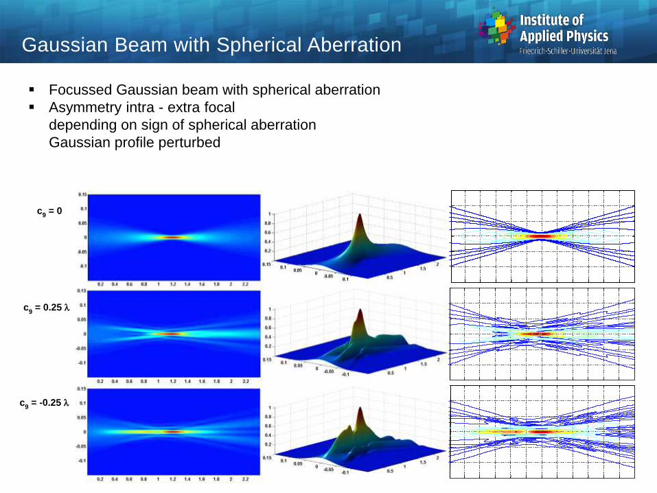
Focussed Gaussian beam with spherical aberration

Asymmetry intra - extra focal

depending on sign of spherical aberration

Gaussian profile perturbed

Gaussian Beam with Spherical Aberration

c9 = -0.25

c9 = 0.25

c9 = 0

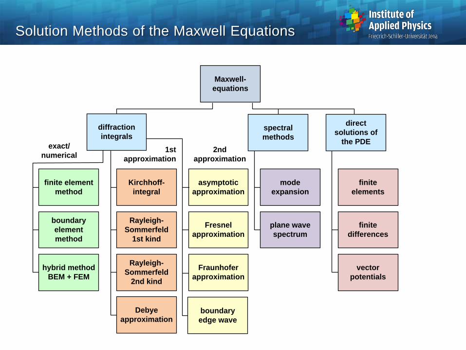
Solution Methods of the Maxwell Equations

Maxwell-

equations

diffraction

integrals

asymptotic

approximation

Fresnel

approximation

Fraunhofer

approximation

finite

elements

finite

differences

exact/

numerical1st

approximation

direct

solutions of

the PDE

spectral

methods

plane wave

spectrum

vector

potentials

2nd

approximation

finite element

method

boundary

element

method

hybrid method

BEM + FEM

Debye

approximation

Kirchhoff-

integral

Rayleigh-

Sommerfeld

1st kind

Rayleigh-

Sommerfeld

2nd kind

mode

expansion

boundary

edge wave

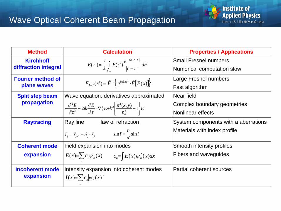
Method Calculation Properties / Applications

Kirchhoff

diffraction integral E r

iE r

e

r rdF

i k r r

FAP

( ) ( ' )'

'

Small Fresnel numbers,

Numerical computation slow

Fourier method of

plane waves )(ˆˆ)'(21 xEFeFxE zvi

II

Large Fresnel numbers

Fast algorithm

Split step beam

propagation

Wave equation: derivatives approximated

En

yxnkE

z

Eik

z

E

o

1

),(2

2

222

2

2

Near field

Complex boundary geometries

Nonlinear effects

Raytracing Ray line law of refraction

r r sj j j j 1 sin '

'sini

n

ni

System components with a aberrations

Materials with index profile

Coherent mode

expansion

Field expansion into modes

n

nn xcxE )()( dxxxEc nn )()( *

Smooth intensity profiles

Fibers and waveguides

Incoherent mode

expansion

Intensity expansion into coherent modes

n

nn xcxI2

)()(

Partial coherent sources

Wave Optical Coherent Beam Propagation

Sampling of the Diffraction Integral

x-6 -4 -2 0 2 4

0

10

20

30

40

50

quadratic

phase

wrapped

phase

2

smallest sampling

intervall

phase

Oscillating exponent :

Fourier transform reduces on 2-

period

Most critical sampling usually

at boundary defines number

of sampling points

Steep phase gradients define the

sampling

High order aberrations are a

problem

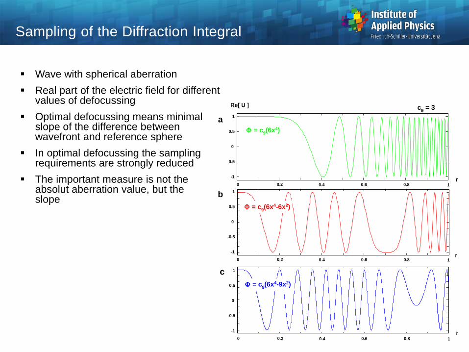
Sampling of the Diffraction Integral

c9 = 3

0 0.2 0.4 0.6 0.8 1

-1

-0.5

0

0.5

1

0 0.2 0.4 0.6 0.8 1

-1

-0.5

0

0.5

1

= c9(6x4-6x2)

r

r

Re[ U ]

= c9(6x4)

0 0.2 0.4 0.6 0.8 1

-1

-0.5

0

0.5

1

r

= c9(6x4-9x2)

a

b

c

Wave with spherical aberration

Real part of the electric field for different values of defocussing

Optimal defocussing means minimal slope of the difference between wavefront and reference sphere

In optimal defocussing the sampling requirements are strongly reduced

The important measure is not the absolut aberration value, but the slope

Propagation by Plane / Spherical Waves

Expansion field in simple-to-propagate waves

1. Spherical waves 2. Plane waves

Huygens principle spectral representation

rdrErr

erE

rrik

2

'

)('

)'(

x

x'

z

E(x)

eikr

r

)(ˆˆ)'( 1 rEFeFrE xy

zik

xyz

x

x'

z

E(x)

eik z z

Kirchhoff diffraction integral in Fresnel approximation

Fourier transform: plan wave expansion

Equivalent form

Curvature removed

Calculation in spherical coordinates

Fresnel Propagation with Equivalence Transform

222 )1(

1'

)1(

)(ˆˆ)'(x

z

Miv

M

zix

Mz

MiM

zik

OO exEFeFeM

exE

x

R<0

z1

z2

starting

plane

observation

plane 1

focus

observation

plane 2

R'<0

R2'>0

x''

x x'

a

a

xxz

i

dxexECxE

2'

)()'(

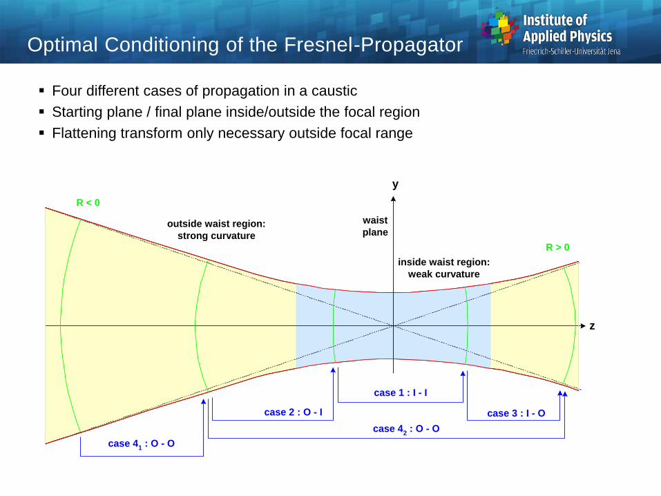
Optimal Conditioning of the Fresnel-Propagator

Four different cases of propagation in a caustic

Starting plane / final plane inside/outside the focal region

Flattening transform only necessary outside focal range

z

y

inside waist region:

weak curvature

outside waist region:

strong curvature

case 1 : I - I

case 42 : O - O

case 41 : O - O

case 2 : O - I case 3 : I - O

waist

plane

R < 0

R > 0

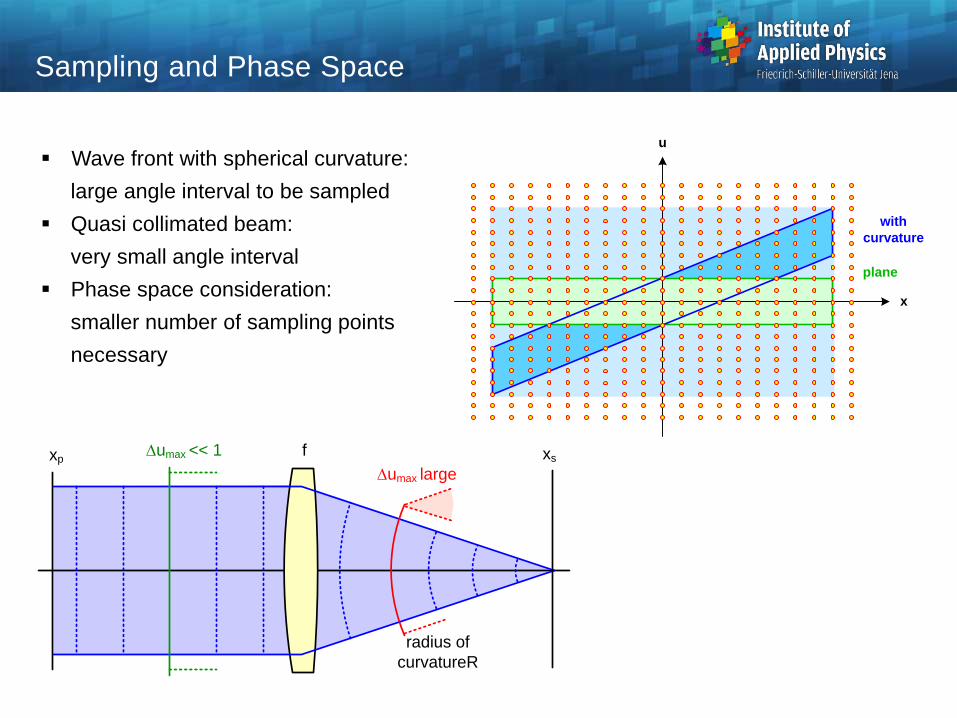
Sampling and Phase Space

x

u

with

curvature

plane

f

radius of

curvatureR

xp xsDumax << 1

Dumax large

Wave front with spherical curvature:

large angle interval to be sampled

Quasi collimated beam:

very small angle interval

Phase space consideration:

smaller number of sampling points

necessary

Setting of initial beam and

sampling parameters

Beam Propagation in Zemax

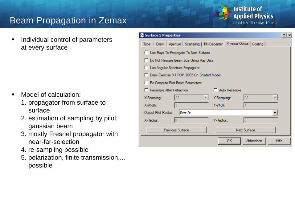
Individual control of parameters

at every surface

Model of calculation:

1. propagator from surface to

surface

2. estimation of sampling by pilot

gaussian beam

3. mostly Fresnel propagator with

near-far-selection

4. re-sampling possible

5. polarization, finite transmission,...

possible

Beam Propagation in Zemax

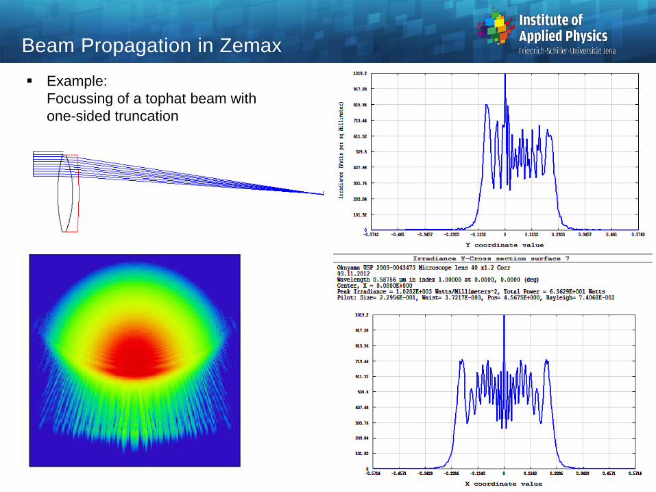
Example:

Focussing of a tophat beam with

one-sided truncation

Beam Propagation in Zemax

Model:

1. definition of a starting polarization

2. every ray carries a Jones vector of polarization, therefore a spatial variation of polarization

is obtained.

3. at any interface, the field is decomposed into s- and p-component in the local system

4. changes of the polarization component due to Fresnel formulas or coatings:

- amplitude, diattenuation

- phase, retardance

Spatial variations of the polarization phase accross the pupil are aberrations,

the interference is influenced and Psf, MTF, Strehl,... are changed

Polarization in Zemax

Starting polarization

Polarization influences:

1. surfaces, by Fresnel formulas or coatings

2. direct input of Jones matrix surfaces with

Polarization in Zemax

EJE

'

y

x

imreimre

imreimre

y

x

y

x

E

E

DiDCiC

BiBAiA

E

E

DC

BA

E

E

'

'

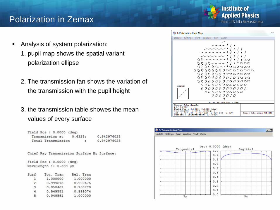
Analysis of system polarization:

1. pupil map shows the spatial variant

polarization ellipse

2. The transmission fan shows the variation of

the transmission with the pupil height

3. the transmission table showes the mean

values of every surface

Polarization in Zemax

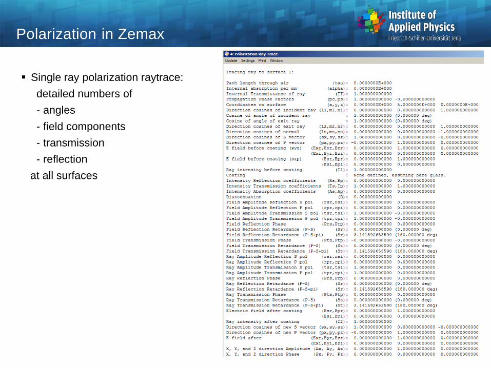
Single ray polarization raytrace:

detailed numbers of

- angles

- field components

- transmission

- reflection

at all surfaces

Polarization in Zemax

Detailed polarization analyses are possible at the individual surfaces by using the coating

menue options

Polarization in Zemax

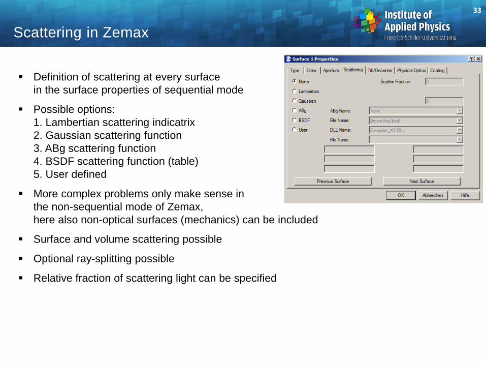
Definition of scattering at every surface

in the surface properties of sequential mode

Possible options:

1. Lambertian scattering indicatrix

2. Gaussian scattering function

3. ABg scattering function

4. BSDF scattering function (table)

5. User defined

More complex problems only make sense in

the non-sequential mode of Zemax,

here also non-optical surfaces (mechanics) can be included

Surface and volume scattering possible

Optional ray-splitting possible

Relative fraction of scattering light can be specified

33

Scattering in Zemax

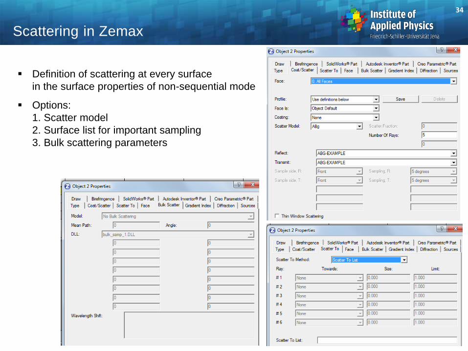
Definition of scattering at every surface

in the surface properties of non-sequential mode

Options:

1. Scatter model

2. Surface list for important sampling

3. Bulk scattering parameters

34

Scattering in Zemax

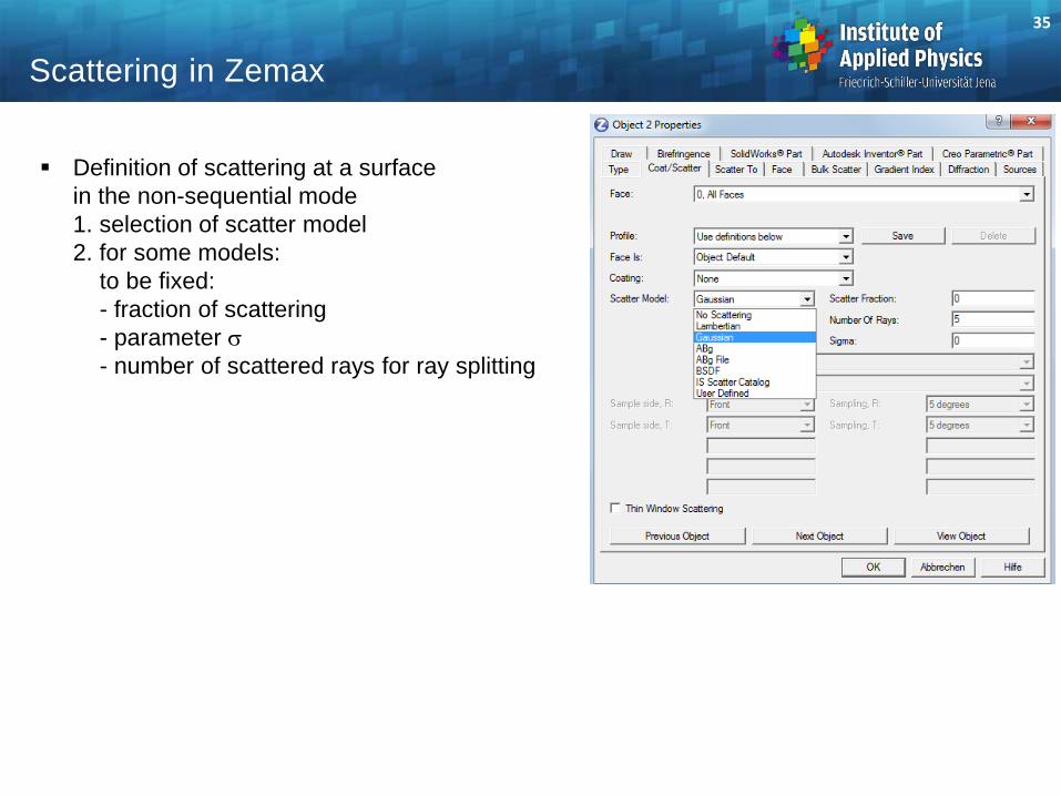
Definition of scattering at a surface

in the non-sequential mode

1. selection of scatter model

2. for some models:

to be fixed:

- fraction of scattering

- parameter s

- number of scattered rays for ray splitting

35

Scattering in Zemax

Surface scattering:

Projection of the scattered ray on the surface, difference to the specular ray: x

Lambertian scattering:

isotropic

Gaussian scattering

ABg model scatter

BSDF by table

Volume scattering: Angle scattering description by probability P

Henyey-Greenstein volume scattering

(biological tissue model)

Rayleigh scattering

Scattering Functions in Zemax

2

2

)( s

x

BSDF eAxF

gBSDFxB

AxF

)(

2/32

2

cos214

1)(

gg

gP

2

4cos1

8

3)( P

( )BSDFF x A

Data file with scattering functions: ABg-data.dat

File can be edited

37

Scattering Tables in Zemax

Tools / Scatter / ABg Scatter Data Catalogs

Specification and definition of scattering

parameters for a new ABg-modell function:

wavelength, angle, A, B, g

Analysis / Scatter viewers / Scatter Function Viewer

Graphical representation of the scattering function

38

Scattering Input and Viewing in Zemax

Acceleration of computational speed:

1. scatter to - option, simple

2. Importance sampling with energy normalization

Importance sampling:

- fixation of a sequence of objects of interest

- only desired directins of rays are considered

- re-scaling of the considered solid angle

- per scattering object a maximum

of 6 target spheres can be

defined

39

Scattering with Importance Sampling

Definition of bulk scattering at the surface

menue

Wavelength shift for fluorescence is possible

Typically angle scattering is assumed

Some DLL-model functions are supported:

1. Mie

2. Rayleigh

3. Henyey-Greenstein

40

Bulk Scattering

Simple example: single focussing lens

Gaussian scattering characteristic at

one surface

Geometrical imaging of a bar pattern

Image with / without Scattering

Scattering must be activated in settings

Blurring increases with growing s-value

41

Scattering Example I

Example from samples with non-sequential mode

Important sampling accelerates the calculation

42

Scattering Example II

Volume scattering example

Stokes shift is possible for fluorescence

43

Scattering Bulk Example