On the performance of Grassmann-covariance-matrix-based spectrumsensing for cognitive radio
PALLAVIRAM SURE
Department of ECE, M S Ramaiah University of Applied Sciences, Bangalore, India
e-mail: [email protected]
MS received 25 October 2020; revised 15 July 2021; accepted 12 August 2021
Abstract. Cognitive radio assures efficient utilization of spectral resources by encouraging opportunistic
spectral access. Its inevitable task of spectrum sensing has been widely addressed in the literature through the
covariance-matrix-computation-based approaches. Unlike these blind approaches, recently a Grassmann
covariance matrix (GCM)-based approach has been devised that requires a priori signal covariance matrix. To
alleviate this impractical limitation, this paper proposes a spectrum sensing approach based on the computation
of a modified projection distance metric on the Grassmann manifold. Particularly, the test statistic is derived
using two GCMs estimated from the received signal frame and the threshold is calculated using Gaussian noise
statistics of the null hypothesis pertaining to the detection problem. Simulations on the signals received in
Rayleigh environments show that the proposed approach renders better probability of detection (Pd) compared
with Covariance Absolute Value (CAV), Akaike Information Criterion (AIC)-based and Maximum Minimum
Eigenvalue (MME) approaches. Performance of the proposed approach is at par with the case when signal
covariance matrix is known a priori. Experiments are conducted using ADALM PLUTO software-defined radio
(SDR) measurements in the ultra-high-frequency (UHF) television (TV) band. Using these measured signals it is
verified that the proposed approach renders Pd ¼ 1 at an SNR of –15 dB compared with the CAV, AIC and
MME approaches, which render Pd ¼ 1 at an SNR of –5 dB.
Keywords. Grassmann covariance matrix; Binet–Cauchy distance; projection distance; blind spectrum
sensing; covariance absolute value; maximum minimum eigenvalue.
1. Introduction
Available licensed radio spectral resources are becom-
ing increasingly insufficient to handle the exponentially
growing demand for wireless services. On the other
hand, some of the licensed radio spectral bands such as
the ultra-high-frequency (UHF) television (TV) band
are heavily underutilized [1]. Cognitive radio emanated
as a promising technology to cater to the needs of
growing wireless services and to improve the spectral
utilization. Owing to its opportunistic spectral access,
the cognitive radio technology ushers the IEEE 802.22
wireless regional area networks (WRAN) [2] where
digital television (DTV) and the wireless microphones
form the licensed primary users (PUs). A cognitive
radio acts as a secondary user (SU) that accesses the
radio channel only when the PU is absent. The SU
vacates the channel as soon as any PU activity gets
detected in the radio channel so as to not cause any
interference to the PU transmissions [3]. To be com-
petent in these crucial functionalities, the SU has to
periodically perform spectrum sensing and detect the
channel’s occupancy.
Spectrum sensing techniques are broadly classified into
two types: Wide-band Spectrum Sensing (WSS) and Nar-
row-band Spectrum Sensing (NSS). WSS techniques scan a
large bandwidth and identify the vacant bands (spectrum
holes), which are in turn used for single or multiple SU
transmissions [4]. Contrarily, NSS techniques detect the
presence or absence of the licensed PU in the given band.
The NSS is usually cast as a binary hypothesis testing
problem. Corresponding test criterion and the threshold are
employed for the detection of channel occupancy. Con-
ventionally, NSS is performed using Energy Detection
(ED) approach [5] where the energy of the received signal
frame is compared to a threshold based on the estimated
noise power. In general, NSS techniques can be classified
as blind and non-blind techniques. Non-blind approaches
such as Matched Filtering [6]-based and the cyclostationary
[7]-based sensing require the knowledge of PU signal pat-
terns and cyclic frequencies, respectively.
Typically, the blind approaches are based on either the
covariance matrix computations as in the Covariance
Absolute Value (CAV) approach [8] or the eigenvalue
computations as in the Maximum Minimum Eigenvalue
(MME) approach [9]. The test criterion of CAV assumes
Sådhanå (2021) 46:222 � Indian Academy of Sciences
https://doi.org/10.1007/s12046-021-01719-9Sadhana(0123456789().,-volV)FT3](0123456789().,-volV)
that the received signal is correlated, and hence compares
the diagonal entries of the covariance matrix to the non-
diagonal entries. The test criterion in the MME approach is
the ratio of the maximum to minimum eigenvalues. Many
other eigenvalue-based approaches have been discussed in
[9], which are variants of the MME approach. The thresh-
olds of signal detection in the CAV and MME approaches
are calculated by fixing the probability of false alarm.
However, the Information Theoretic Criterion (ITC)-based
approaches do not require any fixed probability of false
alarm. Two such approaches employ Akaike Information
Criterion (AIC) and Minimum Description Length (MDL)
criterion for signal detection [10], where the AIC (or MDL)
is computed using all the eigenvalues of the covariance
matrix. The corresponding test criterion compares the first
two AIC (or MDL) values to perform NSS. All these
approaches are suited for SUs with either single or multiple
antennas, and are also employable in a cognitive radio
network (CRN) for cooperative sensing [11].
Recently, mathematical notions of Grassmann manifolds
[12] opened up new possibilities in various science and
engineering applications. Basically, Grassmann manifold is
a space of subspaces that are embedded in a higher
dimensional vector space. Grassmann discriminant analysis
[13] encourages the data to be processed on the Grassmann
manifold. Grassmannian optimization finds its application
in the problem of low-rank matrix completion [14].
Grassmann kernels can also be studied for their replace-
ment in various applications such as traffic state estimation
[15]. Customized deep neural networks have also been
developed for Grassmannian data, referred to as Grassmann
Networks [16], which preserve the manifold geometry.
In wireless communication applications, Grassmannian
learning paradigms have been explored for automatic
recognition of space–time constellations in the design of
intelligent multiple input multiple output (MIMO) com-
munication systems [17]. A detailed survey on several other
applications of Grassmann learning is illustrated in [18].
The topological structure of Grassmann manifolds, and
corresponding distance measures that relate different points
on the manifold, can be employed in NSS to detect the
presence or absence of the PU in DTV bands [19]. In
particular, the dominant eigenspace, termed as Grassmann
covariance matrix (GCM) [20], is computed from the
covariance matrix of the received signal and also the PU’s
signal. A modified Binet–Cauchy distance measure has
been defined as a test statistic and the corresponding
threshold has been derived for a fixed probability of false
alarm, assuming that the covariance matrix of the PU’s
signal is available a priori.
In this paper, the distance measures on the Grassmann
manifold are further explored in the context of NSS.
Particularly, a modified projection distance measure is
proposed as a new test statistic and is analyzed for its
detection capability. Subsequently, we propose a GCM-
based modified NSS approach that relaxes the assumption
on the a priori availability of the PU’s signal covariance
matrix and validate its performance with the proposed test
statistic. The threshold is derived based on the probability
density function (pdf) of the test statistic under the null
hypothesis. Simulations are conducted for NSS using the
ED, CAV, MME, AIC, GCM [19] and the proposed GCM
approaches. The performances of these approaches are
evaluated using probability of detection (Pd) versus the
signal to noise ratio (SNR) and the Pd versus probability
of false alarm plots.
Experiments are conducted by receiving a UHF TV band
signal through the ADALM PLUTO software-defined radio
(SDR), which is transmitted by a distant transmitter
ADALM PLUTO SDR. The signal is captured with a suf-
ficiently good SNR and different noise conditions are
simulated using it. The performances of the previously
discussed NSS approaches have been compared using the
Pd versus SNR plots. By varying the transmit gain of the
ADALM PLUTO SDR, many frames of the received sig-
nals are extracted in the UHF TV band. The results of NSS
approaches on these signals demonstrate that the proposed
approach can yield a Pd performance comparable to that of
the [19], even without the a priori knowledge of the PU’s
signal covariance matrix.
The rest of the paper is organized as follows. Section 2
illustrates the adopted system model and the binary
hypothesis testing problem for signal detection. Further, the
necessary details of Grassmann manifolds are also dis-
cussed. A summary on a few of the existing NSS approa-
ches and the details of the proposed approach are discussed
in section 3 along with the analysis on proposed test
statistic. The simulation and the experimental results are
presented and discussed in section 4 and finally, the paper is
concluded in section 5.
Some of the notations adopted in the rest of the paper are
as follows. Bold faced capital letters represent matrices,
while bold faced small letters indicate vectors. The symbols
:ð ÞT and :ð ÞH represent transpose and Hermitian transpose.
gðxÞ� CN l; r2ð Þ indicates that g(x) is a complex Guassian
random variable with mean l and variance r2. E xf gdenotes the expectation of the random variable x and Pr(.)
represents the probability of an event. The ijth entry of a
matrix A is notated as Aij.
2. System model and Grasmann manifolds
2.1 System model
Consider a SU with a single sensing antenna. Let the dis-
crete time base-band signal received by the SU in a given
time frame be x(n) with a length N and the Nyquist sam-
pling interval be TNy ¼ 1fNy, where fNy is the Nyquist rate.
The signal detection forms a binary hypothesis testing
problem [8], represented as
222 Page 2 of 11 Sådhanå (2021) 46:222

H0 : xðnÞ ¼ eðnÞ n ¼ 0; 1; :::;N � 1
H1 : xðnÞ ¼ rðnÞ þ eðnÞ n ¼ 0; 1; :::;N � 1ð1Þ
with rðnÞ ¼ rðtÞgt¼nTNy; n ¼ 0; 1; :::; ðN � 1Þ being the
Nyquist sampled received signal that had undergone fading
due to the wireless channel and e(n) representing the inde-
pendent, identically distributed (i.i.d.) additive white Gaus-
sian noise (AWGN) samples, eðnÞ� CN 0; r2e� �
. Note that
r(n) can also represent the combined signal received from
multiple PUs. Usually r(n) is correlated owing to the filteringmechanism of the dispersive fading channel, filters and
amplifiers in the radio frequency (RF) chain and the over-
sampling of the signal [8]. For instance, to sense a typical
UHF TV band with 6 MHz bandwidth, the sampling rate is
close to 6 MHz while the actual PU such as the wireless
microphone uses a maximum bandwidth of 200 kHz. Thus,
the received signal is oversampled and hence correlated.
In (1) the null hypothesis H0 represents the absence of
PU’s signal, while H1 indicates the presence of the PU.
Employing a suitable NSS approach, the SU performs
signal detection as shown in figure 1. Signal detection is
accomplished via the decision criterion
TNSS ?H1
H0
kNSS ð2Þ
where TNSS is the test statistic employed in the considered
NSS approach, calculated using the received signal x(n), n 20;N � 1½ � and kNSS is the corresponding threshold. The
detection criterion (2) can be derived using the likelihood
ratio test such as the Neyman–Pearson test [21], by fixing the
probability of false alarm. In general, the performance of any
NSS approach can be assessed using Pd ¼PrðH1=PUpresentÞ versus SNR, for a predefined probability
of false alarm Pfa ¼ PrðH1=PUabsentÞ. Note that Pd
increases with SNR and also with the value of Pfa. An NSS
approach is a valid one if the plot of Pd versus Pfa lies above
the Pd ¼ Pfa line. Hence, both these plots are used as per-
formance measures to compare different NSS approaches.
2.2 Grassmann manifolds
The Grassmann manifold Gðn; kÞ; n� k[ 0 is the space of
all k-dimensional linear subspaces embedded in an n-di-mensional real or complex Euclidean space. Typically, any
element on the Grassmann manifold is represented by an
orthonormal matrix Y 2 Cn�k such that YTY ¼ Ik. Thus,Grassmann manifold [12] is the collection of all such Y,mathematically written as
Gðn; kÞ ¼ span Yð Þ : Y 2 Cn�k;YTY ¼ Ik� � ð3Þ
Note that an element in Gðn; kÞ is invariant to rotations. Thisimplies thatY andYD represent the same point on Gðn; kÞ forany D 2 OðkÞ, the set of all k � k orthonormal matrices. To
characterize the discrepancy between two subspaces (or
points)Y;Z ofGðn; kÞ, the notion of distance between the twoelements is required. Typically, this distance can be expres-
sed in terms of principal angles hi; i ¼ 1; 2; :::; k between
Y;Z [12] and these angles can be computed by performing
singular value decomposition (SVD) as in
YTZ ¼ U cosHð ÞVT ð4Þwhere U, V have the k left and right singular vectors,
respectively, and diagonal entries of cosH ¼diag cos h1; :::; cos hkð Þ are known as canonical correlations.
Some of the distance measures used on Grassmann mani-
folds are Binet–Cauchy distance dBC, projection distance dPand the Chordal distance dC [12], defined as
dBC ¼ 1�Yki¼1
cos2 hi
!1=2
ð5Þ
dP ¼ k �Xki¼1
cos2 hi
!1=2
ð6Þ
dC ¼ffiffiffi2
pk �
Xki¼1
cos hi
!1=2
ð7Þ
Note that the principal angles hi can also be defined as
cos hi ¼ maxui2Y;vi2Z
uTi vi ð8Þ
with ui and vi as the ith columns ofU andV, respectively [18].
The principal angles can be viewed as the minimal angles
between all possible bases of the subspaces of Y and Z.
3. Various NSS approaches and the proposedapproach
In this section, the NSS approaches introduced in section 1
are briefly discussed based on the system model in (1)
followed by the proposed approach.
3.1 Various NSS approaches
The received N-length signal frame xðnÞ; n 2 0;N � 1½ � isdivided into Nss subsegments, each of length L. EachFigure 1. Problem statement: NSS at the SU.
Sådhanå (2021) 46:222 Page 3 of 11 222
subsegment is arranged as xi; i 2 1;Nss½ � of dimension
L� 1. In all the NSS approaches discussed in section 1,
first L� L sample covariance matrix of the received signal
is obtained as
Rxx ¼ 1
Nss
XNss
i¼1
xixHi ð9Þ
3.1.1 CAV approach The CAV approach uses (9) to
calculate the detection criterion [8] as
PLp¼1
PLq¼1
Rxx;pq
�� ��PLp¼1
Rxx;pp
�� �� � kCAV ð10Þ
where Rxx;pq is the pqth element of Rxx and kCAV is the corre-
sponding threshold.To determinekCAV , themeanandvariance
of Rxx;pq are derived forH0 andH1 hypothesis. Using central
limit theorem, the numerator and denominator in the left hand
sideof (10) are found asGaussian distributions [8].ThekCAV isthen evaluated using the definition of Pfa as
kCAV ¼1þ ðL� 1Þ
ffiffiffiffiffiffiffi2
Nssp
q1� Q�1 Pfa
� � ffiffiffiffiffi2Nss
q ð11Þ
with QðaÞ ¼ 1ffiffiffiffi2p
pR1a
e�a2=2da. Observe that by fixing Pfa, the
threshold in (11) can be computed independent of the noise
or signal statistics.
3.1.2 MME approach In the MME approach, the
eigenvalues of (9) are first computed. The ratio of
maximum to minimum eigenvalues is used as the test
statistic and the corresponding decision criterion becomes
amax
amin
� kMME ð12Þ
with amax and amin being the maximum and minimum eigen-
values, respectively. The threshold kMME is derived in [9] as
kMME ¼ffiffiffiffiffiffiffiNss
p þ ffiffiffiL
pffiffiffiffiffiffiffiNss
p � ffiffiffiL
p� 2
1þ BF�11 1� Pfa
� �� � ð13Þ
where F1ðxÞ is the cumulative distribution function of the
Tracy–Widom distribution of order 1 and B ¼ffiffiffiffiffiNss
p þ ffiffiL
pð Þ�2=3
NssLð Þ1=6 .
Similar to that of the CAV approach, the threshold in (13) is
calculated for a fixed Pfa and is independent of the noise or
signal statistics.
3.1.3 AIC approach In the AIC approach, the Leigenvalues of (9) are used to calculate the AIC values
given by
AIC kð Þ ¼ h� 2 log
QLi¼kþ1
a1= L�kð Þi
1L�k
PLi¼kþ1
ai
0BBB@
1CCCA
Nss L�kð Þ
ð14Þ
where h ¼ 2k 2L� kð Þ þ 2, and ai; i 2 1; L½ � are the eigen-
values arranged in decreasing order. The detection proceeds
as
AICð1Þ?H1
H0
AICð2Þ ð15Þ
Note that the detection in (15) is independent of Pfa and no
a priori signal or noise statistics are required for its
computation.
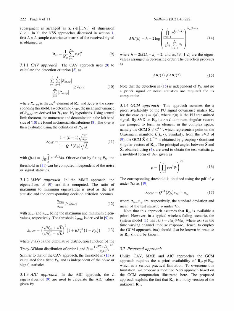
3.1.4 GCM approach This approach assumes the a
priori availability of the PU signal covariance matrix Rss
for the case rðnÞ ¼ sðnÞ, where s(n) is the PU transmitted
signal. By SVD on Rss its r\L dominant singular vectors
are grouped to form an element in the complex space,
namely the GCM �S 2 CL�r, which represents a point on the
Grassmann manifold GðL; rÞ. Similarly, from the SVD of
(9), the GCM �X 2 CL�r is obtained by grouping r dominant
singular vectors of Rxx. The principal angles between �S and�X, obtained using (4), are used to obtain the test statistic q,a modified form of dBC given as
q ¼Yri¼1
cos2hi
!1=2
ð16Þ
The corresponding threshold is obtained using the pdf of qunder H0 as [19]
kGCM ¼ Q�1 Pfa
� �rq0 þ lq0 ð17Þ
where rq0 ; lq0 are, respectively, the standard deviation and
mean of the test statistic q under H0.
Note that this approach assumes that Rss is available a
priori. However, in a typical wireless fading scenario, the
system model (1) has rðnÞ ¼ sðnÞ~hðnÞ where h(n) is the
time varying channel impulse response. Hence, to employ
the GCM approach, h(n) should also be known in practice
or Rrr should be known.
3.2 Proposed approach
Unlike CAV, MME and AIC approaches the GCM
approach requires the a priori availability of Rrr 6¼ Rss,
which is a serious practical limitation. To overcome this
limitation, we propose a modified NSS approach based on
the GCM computation illustrated here. The proposed
approach exploits the fact that Rxx is a noisy version of the
unknown Rrr.
222 Page 4 of 11 Sådhanå (2021) 46:222

Consider the hypothesis H1. Starting from the actual
definition of Rxx, it can be observed that
Rxx ¼ E xixHi
� � ð18Þ
¼ E ri þ eið Þ ri þ eið ÞH� � ð19Þ
¼ E rirHi
� �þ E eieHi
� � ð20Þ
¼ Rrr þ r2eIL ð21Þwhere the third step follows from the fact that ri and ei areuncorrelated [22] and IL is the identity matrix of dimension
L. In a multi-path fading environment we can express
ri ¼ Hsi, where si is the L� 1 subsegment of the PU signal
and H represents the channel matrix [9], following which
Rrr ¼ HRssH�1. The requirement on the estimation of H
confirms that the assumption on a priori availability of Rrr
is impractical. However, (21) indicates that Rxx consists of
a noisy Rrr. Hence, rather than assuming the a priori
availability of Rrr , we propose to estimate it as
R̂rr ¼ Rxx � r2eIL ð22Þwhere noise variance r2e is assumed to be known, as in ED
approach [5]. Further, exploiting the Hermitian Toeplitz
property of Rrr , smoothing is performed to improve its
estimation, as illustrated here. Consider R̂rr of dimension
3� 3, calculated for an N-length received signal. Its
structure is of the form
R̂rr ¼rað0Þ rað1Þ rað2Þr�að1Þ rbð0Þ rbð1Þr�að2Þ r�bð1Þ rcð0Þ
264
375 ð23Þ
Note that the entries in (23) should satisfy Hermitian
Toeplitz property so that R̂rr becomes a valid covariance
matrix. Thus, we compute
rð0Þ ¼ rað0Þ þ rbð0Þ þ rcð0Þ3
ð24Þ
rð1Þ ¼ rað1Þ þ rbð1Þ þ r�að1Þ þ r�bð1Þ� ��4
ð25Þ
rð2Þ ¼ rað2Þ þ r�að2Þ� ��2
ð26Þ
to obtain the modified covariance matrix estimate as
�Rrr ¼rð0Þ rð1Þ rð2Þr�ð1Þ rð0Þ rð1Þr�ð2Þ r�ð1Þ rð0Þ
264
375 ð27Þ
We then propose to extract two GCMs, namely �Sest from
the SVD of �Rrr and �X from the SVD of Rxx, by retaining
r\L dominant singular vectors. As both the GCMs �Sest and
�X represent points on GðL; rÞ, the distance between them
can be measured using the metrics discussed in section 2.
The principal angles /i; i 2 1; r½ � between the two GCMs
are calculated, followed by the computation of the proposed
test statistic
Tprop ¼ 1
r
Xri¼1
cos/i
!ð28Þ
Note that (28) is a modified projection distance unlike the
modified Binet–Cauchy distance employed in [19].
Threshold computation is illustrated here. The pdf of Tprop
under H0 is assumed to be f ðTpropÞ�N mp; r2p
�, which is
later justified from experimental findings. From the
definition
Pfa ¼ PrðH1=PUabsentÞ ð29Þ
¼Z 1
kprop
f ðTpropÞdTprop ð30Þ
where kprop is the required threshold value. Fixing the value
of Pfa and simplifying (30), this threshold can be derived
[21] as
kprop ¼ Q�1 Pfa
� �rp þ mp ð31Þ
where rp;mp need to be obtained from the hypothesis H0.
This GCM-based modified NSS approach is summarized in
table 1. Note that though the proposed approach alleviates
the necessity of a priori Rrr it requires the values of r2e , rpand mp, thus making it a non-blind approach. However,
these values can be easily calculated from the pdf of the test
statistic on the null hypothesis H0. Thus, unlike [19], the
proposed approach does not require a priori Rrr .
Before discussing the simulation and experimental
results of NSS using the proposed approach, the statistical
nature of the proposed test statistic Tprop is worth analyzing.
For this purpose, we simulate a multi-tone analog signal
received from a Rayleigh fading channel and corrupt it with
AWGN of zero mean and known variance. Under the
hypothesis H0 and H1 (SNR of –5 and 0 dB) the plots of
Tprop obtained from 1000 iterations are shown in figure 2,
for different r values.The corresponding pdfs of Tprop under
H0 and H1 (SNR of –5 dB) are also shown in figure 3.
The plots for a fixed r value show that the variance of
Tprop underH0 is more when Rrr is unknown than when it is
known a priori. However, under H1, the variance in both
the cases is almost the same. This can be attributed to the
fact that when signal component is present in x(n), the
estimate of Rrr becomes better. The plots also show that, as
SNR increases, the gap between the mean of Tprop underH1
and that under H0 increases, which implies improved
detection performance at higher SNR values. The plots also
Sådhanå (2021) 46:222 Page 5 of 11 222
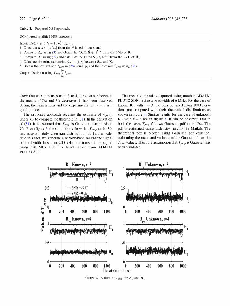
show that as r increases from 3 to 4, the distance between
the means of H0 and H1 decreases. It has been observed
during the simulations and the experiments that r ¼ 3 is a
good choice.
The proposed approach requires the estimate of mp; rpunder H0 to compute the threshold in (31). In the derivation
of (31), it is assumed that Tprop is Gaussian distributed on
H0. From figure 3, the simulations show that Tprop underH0
has approximately Gaussian distribution. To further vali-
date this fact, we generate a narrow-band multi-tone signal
of bandwidth less than 200 kHz and transmit the signal
using 550 MHz UHF TV band carrier from ADALM
PLUTO SDR.
The received signal is captured using another ADALM
PLUTO SDR having a bandwidth of 6 MHz. For the case of
known Rrr with r ¼ 3, the pdfs obtained from 1000 itera-
tions are compared with their theoretical distributions as
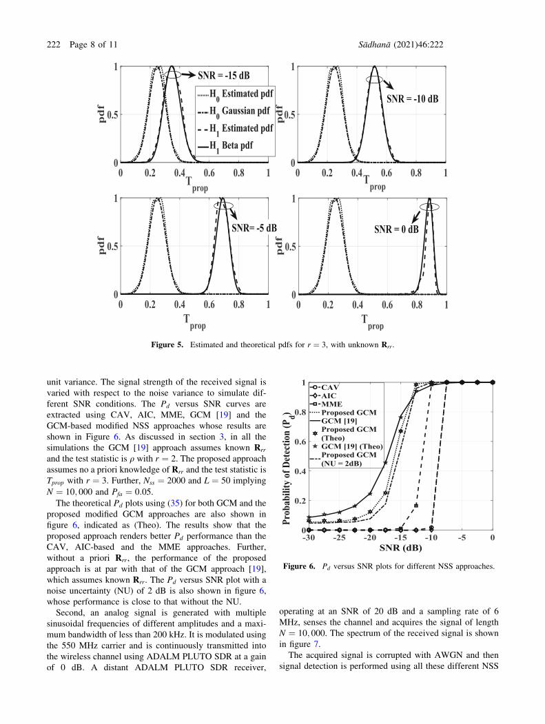
shown in figure 4. Similar results for the case of unknown
Rrr with r ¼ 3 are in figure 5. It can be observed that in
both the cases Tprop follows Gaussian pdf under H0. The
pdf is estimated using ksdensity function in Matlab. The
theoretical pdf is plotted using Gaussian pdf equation,
estimating the mean and variance of the Gaussian fit on the
Tprop values. Thus, the assumption that Tprop is Gaussian has
been validated.
Figure 2. Values of Tprop for H0 and H1.
Table 1. Proposed NSS approach.
GCM-based modified NSS approach
Input: xðnÞ; n 2 0;N � 1½ �, r2e , rp, mp
1. Construct xi; i 2 1;Nss½ � from the N-length input signal
2. Compute Rxx using (9) and obtain the GCM �X 2 RL�r from the SVD of Rxx.
3. Compute Rrr using (22) and calculate the GCM �Sest 2 RL�r from the SVD of �Rrr
4. Calculate the principal angles /i; i 2 1; r½ � between �Sest and �X.5. Obtain the test statistic Tprop in (28) using /i and the threshold kprop using (31).
Output: Decision using Tprop ?H1
H0
kprop
222 Page 6 of 11 Sådhanå (2021) 46:222
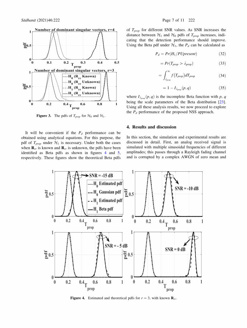
It will be convenient if the Pd performance can be
obtained using analytical equations. For this purpose, the
pdf of Tprop under H1 is necessary. Under both the cases
when Rrr is known and Rrr is unknown, the pdfs have been
identified as Beta pdfs as shown in figures 4 and 5,
respectively. These figures show the theoretical Beta pdfs
of Tprop for different SNR values. As SNR increases the
distance between H1 and H0 pdfs of Tprop increases, indi-
cating that the detection performance should improve.
Using the Beta pdf under H1, the Pd can be calculated as
Pd ¼ PrðH1=PUpresentÞ ð32Þ
¼ PrðTprop [ kpropÞ ð33Þ
¼Z 1
kprop
f Tprop� �
dTprop ð34Þ
¼ 1� Ikpropðp; qÞ ð35Þwhere Ikpropðp; qÞ is the incomplete Beta function with p, q
being the scale parameters of the Beta distribution [23].
Using all these analysis results, we now proceed to explore
the Pd performance of the proposed NSS approach.
4. Results and discussion
In this section, the simulation and experimental results are
discussed in detail. First, an analog received signal is
simulated with multiple sinusoidal frequencies of different
amplitudes; this passes through a Rayleigh fading channel
and is corrupted by a complex AWGN of zero mean and
Figure 3. The pdfs of Tprop for H0 and H1.
Figure 4. Estimated and theoretical pdfs for r ¼ 3, with known Rrr .
Sådhanå (2021) 46:222 Page 7 of 11 222
unit variance. The signal strength of the received signal is
varied with respect to the noise variance to simulate dif-
ferent SNR conditions. The Pd versus SNR curves are
extracted using CAV, AIC, MME, GCM [19] and the
GCM-based modified NSS approaches whose results are
shown in Figure 6. As discussed in section 3, in all the
simulations the GCM [19] approach assumes known Rrr
and the test statistic is q with r ¼ 2. The proposed approach
assumes no a priori knowledge of Rrr and the test statistic is
Tprop with r ¼ 3. Further, Nss ¼ 2000 and L ¼ 50 implying
N ¼ 10; 000 and Pfa ¼ 0:05.The theoretical Pd plots using (35) for both GCM and the
proposed modified GCM approaches are also shown in
figure 6, indicated as (Theo). The results show that the
proposed approach renders better Pd performance than the
CAV, AIC-based and the MME approaches. Further,
without a priori Rrr, the performance of the proposed
approach is at par with that of the GCM approach [19],
which assumes known Rrr. The Pd versus SNR plot with a
noise uncertainty (NU) of 2 dB is also shown in figure 6,
whose performance is close to that without the NU.
Second, an analog signal is generated with multiple
sinusoidal frequencies of different amplitudes and a maxi-
mum bandwidth of less than 200 kHz. It is modulated using
the 550 MHz carrier and is continuously transmitted into
the wireless channel using ADALM PLUTO SDR at a gain
of 0 dB. A distant ADALM PLUTO SDR receiver,
operating at an SNR of 20 dB and a sampling rate of 6
MHz, senses the channel and acquires the signal of length
N ¼ 10; 000. The spectrum of the received signal is shown
in figure 7.
The acquired signal is corrupted with AWGN and then
signal detection is performed using all these different NSS
Figure 5. Estimated and theoretical pdfs for r ¼ 3, with unknown Rrr .
Figure 6. Pd versus SNR plots for different NSS approaches.
222 Page 8 of 11 Sådhanå (2021) 46:222

approaches. The obtained Pd versus SNR plots are shown in
figure 8. These results show that the performance of the
proposed approach is at par with that of GCM approach
[19] even when Rrr is unknown. Further, the Region of
Operating Characteristic (ROC) curves namely the Pd
versus Pfa plots are shown in figure 9 for the GCM [19] and
the proposed approach. At SNR of –10 dB and also –20 dB
the plots lie above the Pd ¼ Pfa line, thus validating their
detection performances. At an SNR of –10 dB, the pro-
posed approach and the GCM approach [19] have negligi-
ble difference in the Pd. At –20 dB SNR, the proposed
approach has slightly lower Pd than the GCM approach
[19].
Third, to validate the performance of the proposed
approach experimentally, a UHF wireless link is set up as
shown in figure 10. The transmitter ADALM PLUTO is
programmed to continuously transmit a multi-frequency
sinusoid of maximum frequency less than 200 kHz, which
is modulated using a 550 MHz carrier signal for a desired
gain value. The receiver ADALM PLUTO is placed at a
distance of 2 m, which receives the 550 MHz signal at a
sampling rate of 6 MHz and has a fixed gain of 20 dB. The
gain of the transmitter is varied from –30 to 0 dB, in steps
of 5 dB.
At each gain setting the receiver captures Miter ¼ 430
frames of the received signal, where each frame x(n) has alength of N ¼ 10; 000. Signal detection is performed on
each frame using CAV, AIC, MME, GCM [19] and the
proposed GCM-based NSS approaches. The probability of
detection for each gain setting is then calculated as
Pd ¼ # TNSS [ kNSSð ÞMiter
ð36Þ
where # TNSS [ kNSSð Þ indicates the number of times
TNSS [ kNSS. The experimental results of Pd versus SNR are
shown in figure 11. These results are obtained with Pfa ¼0:05 and L ¼ 200. In the case of GCM [19] Rrr is pre-
computed, while lq0 , rq0 are estimated from H0. For the
proposed modified GCM approach the Rrr is assumed to be
unknown, while r2e , mp and rp are estimated from H0. The
transmitter is switched off to represent H0 and several
frames of the received signal are acquired, each with aFigure 7. Received spectrum acquired from ADALM PLUTO.
Figure 8. Simulated Pd versus SNR plots for acquired signal
with different NSS approaches.
Figure 9. Pd versus Pfa plots for SNR of –10 and –20 dB.
Figure 10. Setup of UHF wireless link.
Sådhanå (2021) 46:222 Page 9 of 11 222
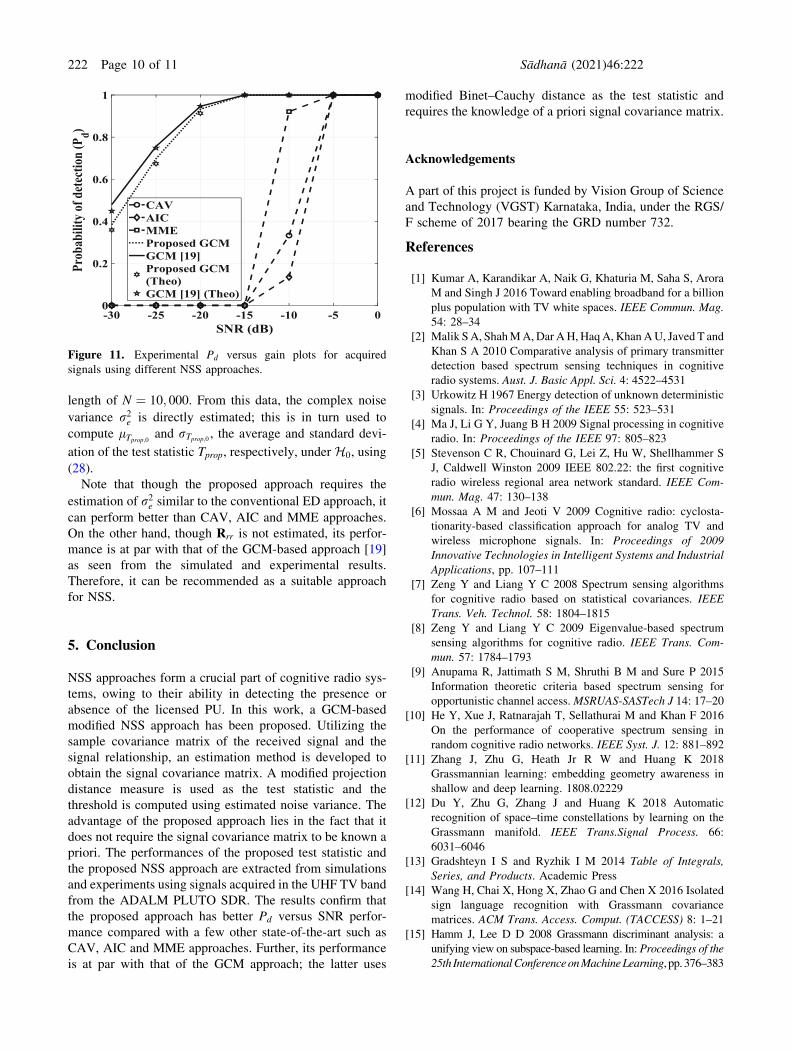
length of N ¼ 10; 000. From this data, the complex noise
variance r2e is directly estimated; this is in turn used to
compute lTprop;0 and rTprop;0 , the average and standard devi-
ation of the test statistic Tprop, respectively, under H0, using
(28).
Note that though the proposed approach requires the
estimation of r2e similar to the conventional ED approach, it
can perform better than CAV, AIC and MME approaches.
On the other hand, though Rrr is not estimated, its perfor-
mance is at par with that of the GCM-based approach [19]
as seen from the simulated and experimental results.
Therefore, it can be recommended as a suitable approach
for NSS.
5. Conclusion
NSS approaches form a crucial part of cognitive radio sys-
tems, owing to their ability in detecting the presence or
absence of the licensed PU. In this work, a GCM-based
modified NSS approach has been proposed. Utilizing the
sample covariance matrix of the received signal and the
signal relationship, an estimation method is developed to
obtain the signal covariance matrix. A modified projection
distance measure is used as the test statistic and the
threshold is computed using estimated noise variance. The
advantage of the proposed approach lies in the fact that it
does not require the signal covariance matrix to be known a
priori. The performances of the proposed test statistic and
the proposed NSS approach are extracted from simulations
and experiments using signals acquired in the UHF TV band
from the ADALM PLUTO SDR. The results confirm that
the proposed approach has better Pd versus SNR perfor-
mance compared with a few other state-of-the-art such as
CAV, AIC and MME approaches. Further, its performance
is at par with that of the GCM approach; the latter uses
modified Binet–Cauchy distance as the test statistic and
requires the knowledge of a priori signal covariance matrix.
Acknowledgements
A part of this project is funded by Vision Group of Science
and Technology (VGST) Karnataka, India, under the RGS/
F scheme of 2017 bearing the GRD number 732.
References
[1] Kumar A, Karandikar A, Naik G, Khaturia M, Saha S, Arora
M and Singh J 2016 Toward enabling broadband for a billion
plus population with TV white spaces. IEEE Commun. Mag.54: 28–34
[2] Malik SA, ShahMA,Dar AH,HaqA,KhanAU, Javed T and
Khan S A 2010 Comparative analysis of primary transmitter
detection based spectrum sensing techniques in cognitive
radio systems. Aust. J. Basic Appl. Sci. 4: 4522–4531[3] Urkowitz H 1967 Energy detection of unknown deterministic
signals. In: Proceedings of the IEEE 55: 523–531
[4] Ma J, Li G Y, Juang B H 2009 Signal processing in cognitive
radio. In: Proceedings of the IEEE 97: 805–823
[5] Stevenson C R, Chouinard G, Lei Z, Hu W, Shellhammer S
J, Caldwell Winston 2009 IEEE 802.22: the first cognitive
radio wireless regional area network standard. IEEE Com-mun. Mag. 47: 130–138
[6] Mossaa A M and Jeoti V 2009 Cognitive radio: cyclosta-
tionarity-based classification approach for analog TV and
wireless microphone signals. In: Proceedings of 2009Innovative Technologies in Intelligent Systems and IndustrialApplications, pp. 107–111
[7] Zeng Y and Liang Y C 2008 Spectrum sensing algorithms
for cognitive radio based on statistical covariances. IEEETrans. Veh. Technol. 58: 1804–1815
[8] Zeng Y and Liang Y C 2009 Eigenvalue-based spectrum
sensing algorithms for cognitive radio. IEEE Trans. Com-mun. 57: 1784–1793
[9] Anupama R, Jattimath S M, Shruthi B M and Sure P 2015
Information theoretic criteria based spectrum sensing for
opportunistic channel access.MSRUAS-SASTech J 14: 17–20[10] He Y, Xue J, Ratnarajah T, Sellathurai M and Khan F 2016
On the performance of cooperative spectrum sensing in
random cognitive radio networks. IEEE Syst. J. 12: 881–892[11] Zhang J, Zhu G, Heath Jr R W and Huang K 2018
Grassmannian learning: embedding geometry awareness in
shallow and deep learning. 1808.02229
[12] Du Y, Zhu G, Zhang J and Huang K 2018 Automatic
recognition of space–time constellations by learning on the
Grassmann manifold. IEEE Trans.Signal Process. 66:
6031–6046
[13] Gradshteyn I S and Ryzhik I M 2014 Table of Integrals,Series, and Products. Academic Press
[14] Wang H, Chai X, Hong X, Zhao G and Chen X 2016 Isolated
sign language recognition with Grassmann covariance
matrices. ACM Trans. Access. Comput. (TACCESS) 8: 1–21[15] Hamm J, Lee D D 2008 Grassmann discriminant analysis: a
unifying view on subspace-based learning. In: Proceedings of the25th InternationalConferenceonMachineLearning, pp. 376–383
Figure 11. Experimental Pd versus gain plots for acquired
signals using different NSS approaches.
222 Page 10 of 11 Sådhanå (2021) 46:222

[16] Bishnu A, Bhatia V 2018 Grassmann manifold-based
spectrum sensing for TV white spaces. IEEE Trans. Cogni-tive Commun. Network. 4: 462–472
[17] Harandi M T, Sanderson C, Shirazi S and Lovell B C 2011
Graph embedding discriminant analysis on Grassmannian
manifolds for improved image set matching. In: Proceedingsof CVPR IEEE 2011, pp. 2705–2712
[18] Dai W, Kerman E and Milenkovic O 2012 A geometric
approach to low-rank matrix completion. IEEE Trans. Inf.Theory 58: 237–247
[19] Huang Z, Wu J and Van G L 2018 Building deep networks
on Grassmann manifolds. In: Proceedings of the AAAIConference on Artificial Intelligence 32
[20] Narendra Babu C, Sure P, Bhuma C M 2020 Sparse Bayesian
learning assisted approaches for road network traffic state
estimation. IEEE Trans. Intell. Transp. Syst. 22: 1733–1741[21] Chandrala M S, Hadli P, Aishwarya R, Jejo Kevin C, Sunil Y
and Sure P 2019 A GUI for wideband spectrum sensing using
compressive sampling approaches. In: Proceedings of the 10thInternational Conference on Computing, Communication andNetworking Technologies (ICCCNT), IEEE, pp. 1–6
[22] Kay Steven M 1998 Detection Theory. Fundamentals ofStatistical Signal Processing, vol. II. Prentice-Hall PTR,
pp. 1545–5971
[23] Goldsmith A 2005 Wireless Communications. Cambridge
University Press
Sådhanå (2021) 46:222 Page 11 of 11 222
Recommended


