Covariance Matrix Applications

Dimensionality Reduction

Outline

• What is the covariance matrix?

• Example

• Properties of the covariance matrix

• Spectral Decomposition – Principal Component Analysis

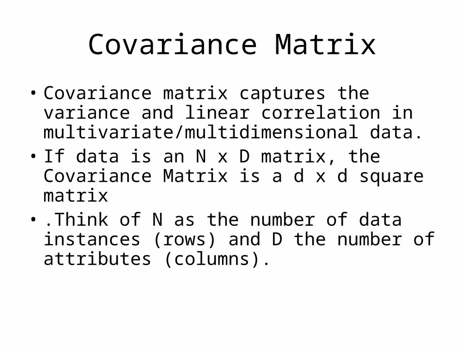
Covariance Matrix

• Covariance matrix captures the variance and linear correlation in multivariate/multidimensional data.

• If data is an N x D matrix, the Covariance Matrix is a d x d square matrix

• .Think of N as the number of data instances (rows) and D the number of attributes (columns).

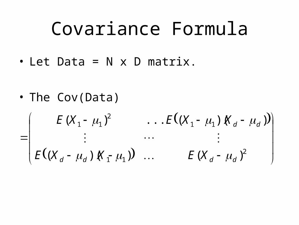
Covariance Formula

• Let Data = N x D matrix.

• The Cov(Data)

211

112

11

)())((

))((...)(

dddd

dd

XEXXE

XXEXE

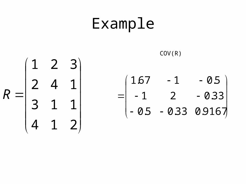
Example

214

113

142

321

R

9167.033.05.0

33.021

5.0167.1

COV(R)

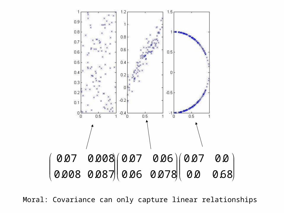
68.00.0

0.007.0

078.006.0

06.007.0

087.0008.0

008.007.0

Moral: Covariance can only capture linear relationships

Dimensionality Reduction

• If you work in “data analytics” it is common these days to be handed a data set which has lots of variables (dimensions).

• The information in these variables is often redundant – there are only a few sources of genuine information.

• Question: How can be identify these sources automatically?

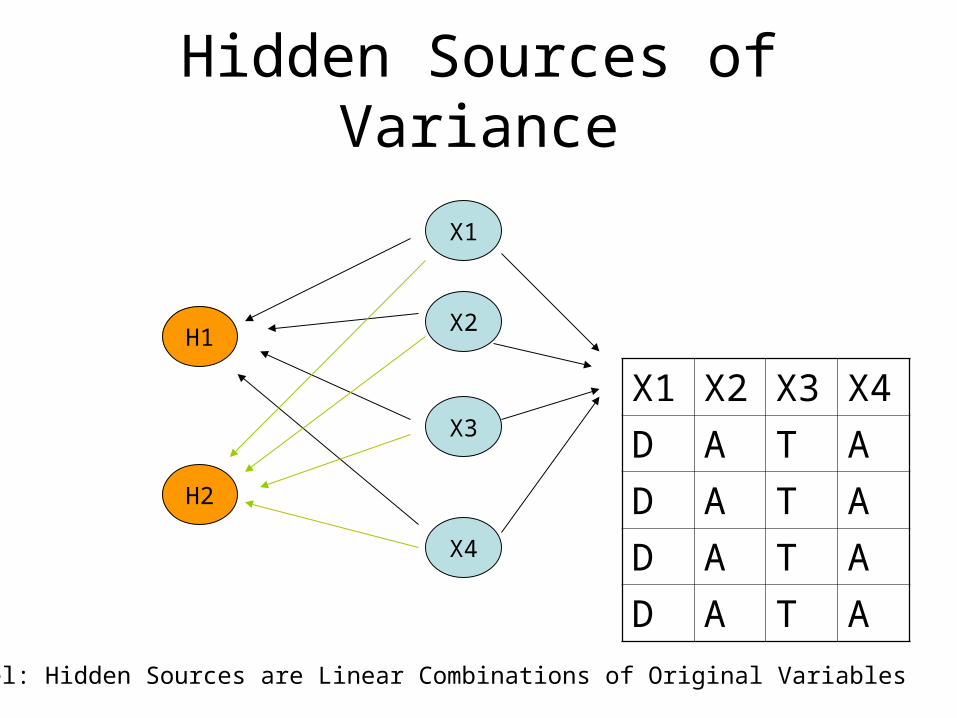
Hidden Sources of Variance

X1

X2

X3

X4

H2

H1

X1 X2 X3 X4

D A T A

D A T A

D A T A

D A T A

Model: Hidden Sources are Linear Combinations of Original Variables

Hidden Sources

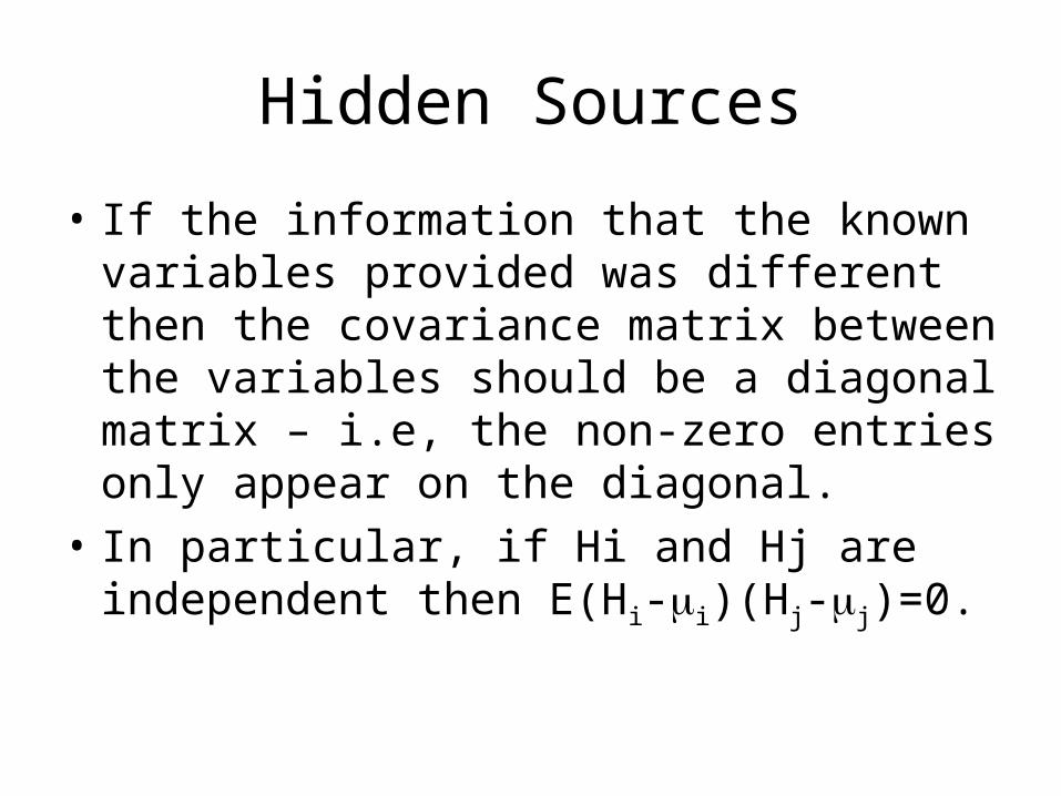
• If the information that the known variables provided was different then the covariance matrix between the variables should be a diagonal matrix – i.e, the non-zero entries only appear on the diagonal.

• In particular, if Hi and Hj are independent then E(Hi-i)(Hj-j)=0.

Hidden Sources

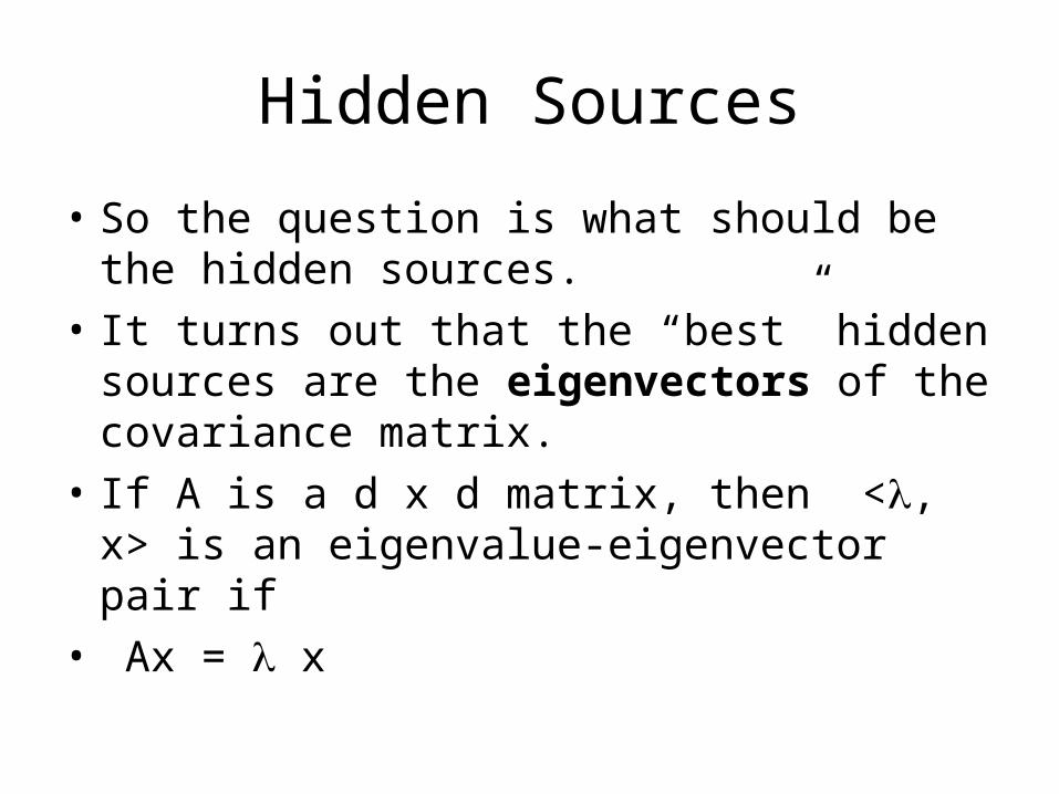
• So the question is what should be the hidden sources.

• It turns out that the “best” hidden sources are the eigenvectors of the covariance matrix.

• If A is a d x d matrix, then <, x> is an eigenvalue-eigenvector pair if

• Ax = x

Explanation

We have two axis, X1 and X2. We want to project the data along the directionof maximum variance.

a

Covariance Matrix Properties

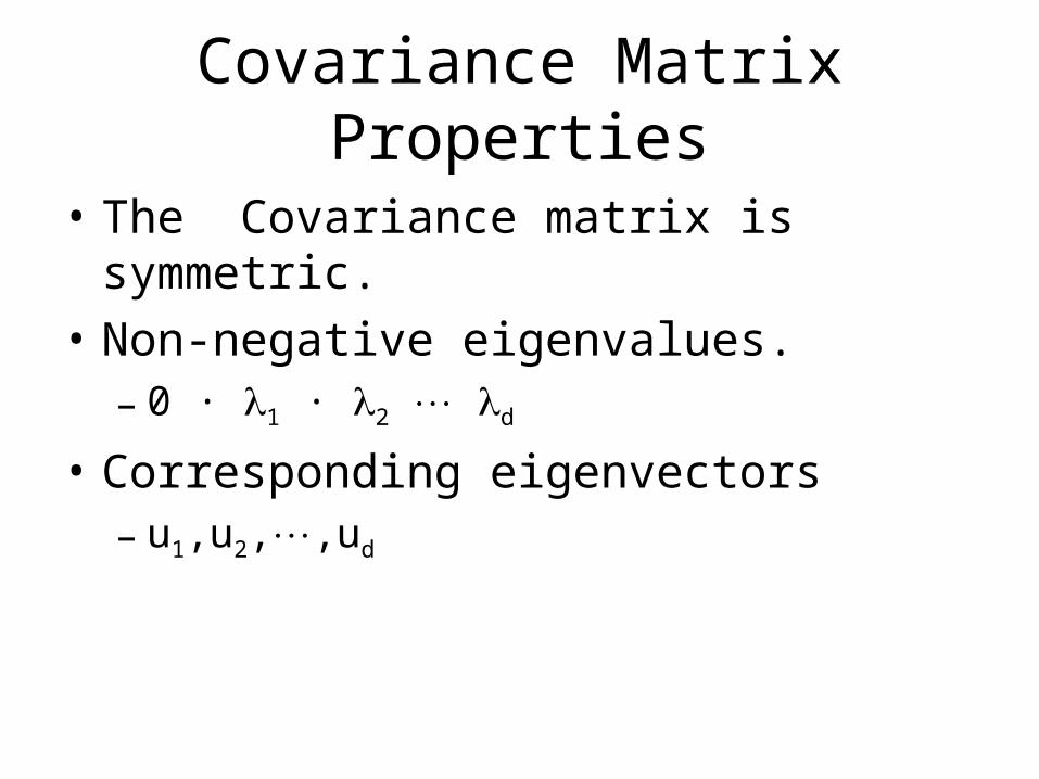
• The Covariance matrix is symmetric.

• Non-negative eigenvalues. – 0 · 1 · 2 d

• Corresponding eigenvectors– u1,u2,,ud

Principal Component Analysis

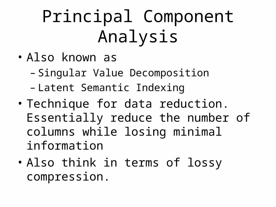
• Also known as– Singular Value Decomposition– Latent Semantic Indexing

• Technique for data reduction. Essentially reduce the number of columns while losing minimal information

• Also think in terms of lossy compression.

Motivation

• Bulk of data has a time component

• For example, retail transactions, stock prices

• Data set can be organized as N x M table

• N customers and the price of the calls they made in 365 days

• M << N

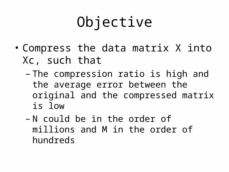
Objective

• Compress the data matrix X into Xc, such that– The compression ratio is high and the

average error between the original and the compressed matrix is low

– N could be in the order of millions and M in the order of hundreds

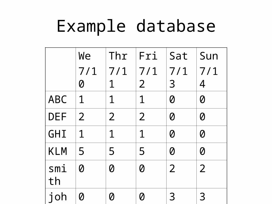
Example database

We

7/10

Thr

7/11

Fri

7/12

Sat

7/13

Sun

7/14

ABC 1 1 1 0 0

DEF 2 2 2 0 0

GHI 1 1 1 0 0

KLM 5 5 5 0 0

smith

0 0 0 2 2

john 0 0 0 3 3

tom 0 0 0 1 1

Decision Support Queries

• What was the amount of sales to GHI on July 11?

• Find the total sales to business customers for the week ending July 12th?

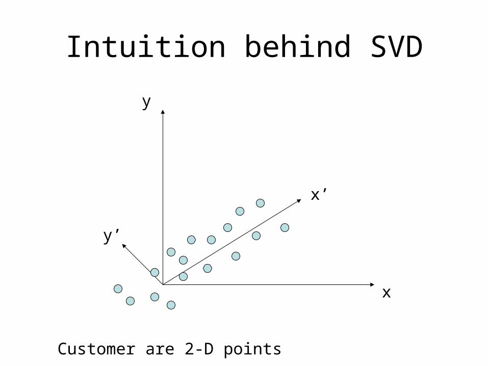
Intuition behind SVD

x

y

x’

y’

Customer are 2-D points

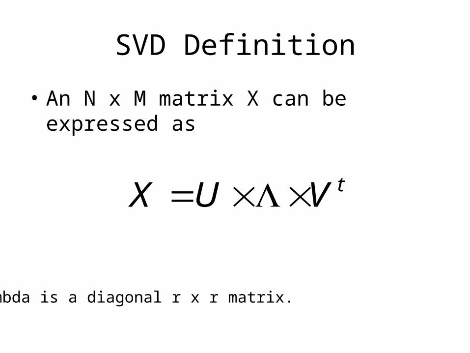
SVD Definition

• An N x M matrix X can be expressed as

tVUX

Lambda is a diagonal r x r matrix.

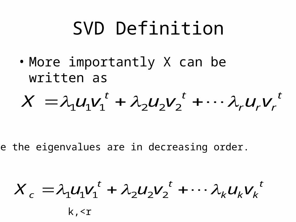
SVD Definition

• More importantly X can be written as

trrr

tt vuvuvuX 222111

Where the eigenvalues are in decreasing order.

tkkk

ttc vuvuvuX 222111

k,<r

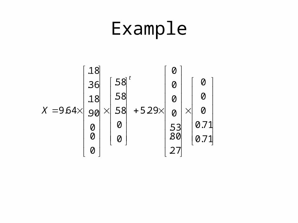
Example

71.0

71.0

0

0

0

27.

80.53.

0

0

0

0

29.5

0

0

58.

58.

58.

0

00

90.

18.

36.

18.

64.9

t

X

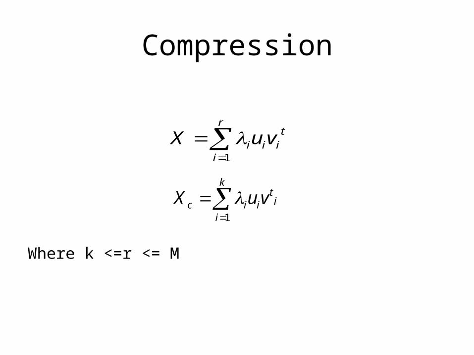
Compression

tii

r

ii vuX

1

it

k

iiic vuX

1

Where k <=r <= M