REPORT No.
12-02
OCEAN ENGINEERING GROUP
Three Dimensional Viscous/Inviscid Interactive Method
and Its Application to Propeller Blades
Xiangming Yu
August 2012
ENVIRONMENTAL AND WATER RESOURCES ENGINEERING
DEPARTMENT OF CIVIL, ARCHITECTURAL AND ENVIRONMENTAL ENG.
THE UNIVERSITY OF TEXAS AT AUSTIN
AUSTIN, TX 78712

Copyright
by
Xiangming Yu
2012

The Thesis Committee for Xiangming Yucertifies that this is the approved version of the following thesis:
Three Dimensional Viscous/Inviscid Interactive
Method and Its Application to Propeller Blades
Committee:
Spyros A. Kinnas, Supervisor
Howard Liljestrand

Three Dimensional Viscous/Inviscid Interactive
Method and Its Application to Propeller Blades
by
Xiangming Yu, B.E.
THESIS
Presented to the Faculty of the Graduate School of
The University of Texas at Austin
in Partial Fulfillment
of the Requirements
for the Degree of
MASTER OF SCIENCE in ENGINEERING
THE UNIVERSITY OF TEXAS AT AUSTIN
August 2012

Dedicated to my family and friends.

Acknowledgments
I first wish to thank my supervisor, Prof. Kinnas, for his continued
guidance and assistance over the last two years. His extraordinary wisdom
and unlimited passion for research inspires me to pursue my own academic
career. His encouragements and suggestions lead me forward, and help me
overcome difficulties in both my research and life. I do and will benefit from
him all my life. Also I want to thank Prof. Liljestrand for his reviewing of my
thesis.
Then I would like to thank all my friends in the Computational Hy-
drodynamics Laboratory (CHL) for their selfless help and companionship. I
would especially thank Mr. Ye Tian, Shu-Hao Chang, Liwei Han and Dr. Lei
He for their significant help not only in my research, but also in many aspects
of my life.
I would also thank my friends at Austin: Mr. Wentao Fu, Xudong Xu,
Haizhao Yang, Shichao Dai and Miss Xiaoqian Li. My life at Austin becomes
more colorful and memorable because of their companionship.
Finally, I want to express my sincere appreciation to my parents, Xi-
aosheng Yu and Guixia Liu. Without their love and encouragement, I would
never finish this work.
This work was supported by the U.S. Office of Naval Research (Con-
v

tracts N00014-07-1-0616 and N00014-10-1-0931) and members of the Phases V
and VI of the Consortium on Cavitation Performance of High Speed Propul-
sors: American Bureau of Shipping, Kawasaki Heavy Industry Ltd., Rolls-
Royce Marine AB, Rolls-Royce Marine AS, SSPA AB, Andritz Hydro GmbH,
Wartsilaa Netherlands B.V., Wartsilaa Norway AS, Wartsilaa Lips Defense
S.A.S., Wartsilaa CME Zhenjiang Propeller Co. Ltd, Daewoo Shipbuilding &
Marine Engineering Co., Ltd. and Samsung Heavy Industries Co., Ltd.
vi

Three Dimensional Viscous/Inviscid Interactive
Method and Its Application to Propeller Blades
Publication No.
Xiangming Yu, M.S.E.
The University of Texas at Austin, 2012
Supervisor: Spyros A. Kinnas
A three dimensional viscous/inviscid interactive boundary layer method
for predicting the effects of fluid viscosity on the performance of fully wetted
propellers is presented. This method is developed by coupling a three dimen-
sional low-order potential based panel method and a two dimensional integral
boundary layer analysis method. To simplify the solution procedures, this
method applies a reasonable assumption that the effects of the boundary lay-
er along the span wise direction (radially outward for propeller blades) could
be negligible compared with those along the stream wise direction (constant
radius for propeller blades). One significant development of this method, com-
pared with previous work, is to completely consider the effects of the added
sources on the whole blades and wakes rather than evaluate the boundary lay-
er effects along each strip, without interaction among strips. This method is
applied to Propeller DTMB 4119, Propeller NSRDC 4381 and DTMB Duct II
vii
for validation. The results show good correlation with experimental measure-
ments or RANS (ANSYS/FLUENT) results. The method is further used to
develop a viscous image model for the cases of three dimensional wing blades
between two parallel slip walls.
An improved method for hydrofoils and propeller blades with non-zero
thickness or open trailing edges is presented as well. The method in this thesis
follows the idea of Pan (2009, 2011), but applies a new extension scheme, which
uses second order polynomials to describe the extension edges. A improved
simplified search scheme is also used to find the correct shape of the extension
automatically to ensure the two conditions are satisfied.
viii
Table of Contents
Acknowledgments v
Abstract vii
List of Tables xii
List of Figures xiii
Nomenclature xxii
Chapter 1. Introduction 1
1.1 Background . . . . . . . . . . . . . . . . . . . . . . . . . . . . 1
1.2 Objective . . . . . . . . . . . . . . . . . . . . . . . . . . . . . . 3
1.3 Organization . . . . . . . . . . . . . . . . . . . . . . . . . . . . 3
Chapter 2. Two Dimensional Viscous/Inviscid Interactive Method 5
2.1 Governing Equations . . . . . . . . . . . . . . . . . . . . . . . 5
2.2 Boundary Conditions . . . . . . . . . . . . . . . . . . . . . . . 6
2.3 2D Wall Transpiration Model . . . . . . . . . . . . . . . . . . . 7
2.3.1 Boundary Layer Simulation . . . . . . . . . . . . . . . . 7
2.3.2 Edge Velocity Expression . . . . . . . . . . . . . . . . . 8
2.4 The Viscous/Inviscid Flow Coupling . . . . . . . . . . . . . . . 14
2.4.1 2D Integral Boundary Layer Equations . . . . . . . . . . 14
2.4.2 Coupling Algorithm . . . . . . . . . . . . . . . . . . . . 15
2.5 2D Viscous Hydrofoil Case . . . . . . . . . . . . . . . . . . . . 15
2.5.1 Method Validation . . . . . . . . . . . . . . . . . . . . . 17
2.5.2 Result Comparison with RANS (ANSYS/FLUENT) . . 19
ix

Chapter 3. Three Dimensional Viscous/Inviscid Interactive Method 28
3.1 Assumption . . . . . . . . . . . . . . . . . . . . . . . . . . . . 29
3.2 3D Wall Transpiration Model . . . . . . . . . . . . . . . . . . . 35
3.2.1 One Blade . . . . . . . . . . . . . . . . . . . . . . . . . 35
3.2.2 Multiple Blades . . . . . . . . . . . . . . . . . . . . . . 37
3.3 Propeller DTMB4119 . . . . . . . . . . . . . . . . . . . . . . . 39
3.4 Propeller NSRDC4381 . . . . . . . . . . . . . . . . . . . . . . 48
3.5 DTMB Duct II . . . . . . . . . . . . . . . . . . . . . . . . . . 62
Chapter 4. Viscous Image Model 68
4.1 Image Model with Panel Method Only . . . . . . . . . . . . . 68
4.2 Image Model with 3D Viscous/Inviscid Interactive Method . . 71
4.3 Straight Wing between Two Parallel Slip Walls . . . . . . . . . 72
4.4 Swept Wing between Two Parallel Slip Walls . . . . . . . . . . 81
Chapter 5. Hydrofoils and Propellers with Non-Zero TrailingEdge Thickness 86
5.1 2D Hydrofoils with Non-Zero Trailing Edge Thickness . . . . . 86
5.1.1 Open Trailing Edge Extension Scheme . . . . . . . . . . 86
5.1.2 Search Scheme for Extension . . . . . . . . . . . . . . . 89
5.2 Sample Cases of 2D Hydrofoils . . . . . . . . . . . . . . . . . 91
5.2.1 Strip of ONR-AxWj-2 Rotor Blade . . . . . . . . . . . . 91
5.2.2 NACA Hydrofoil . . . . . . . . . . . . . . . . . . . . . . 95
5.3 Propeller Blades with Non-zero Trailing Edge Thickness . . . . 98
Chapter 6. Conclusions and Recommendations 107
6.1 Conclusions . . . . . . . . . . . . . . . . . . . . . . . . . . . . 107
6.2 Recommendations . . . . . . . . . . . . . . . . . . . . . . . . . 109
Appendix 111
Appendix 1. Evaluation of Influence Coefficients 112
1.1 2D Influence Coefficients . . . . . . . . . . . . . . . . . . . . . 112
1.2 3D Influence Coefficients . . . . . . . . . . . . . . . . . . . . . 112
x

Bibliography 113
Vita 118
xi
List of Tables
2.1 Three grids used for the grid dependency study of the RANS(ANSYS/FLUENT) case for 2D hydrofoil . . . . . . . . . . . . 22
2.2 Information of the RANS (ANSYS/FLUENT) case for 2D hy-drofoil . . . . . . . . . . . . . . . . . . . . . . . . . . . . . . . 23
3.1 Information of the RANS (ANSYS/FLUENT) case for Pro-peller NSRDC4381 . . . . . . . . . . . . . . . . . . . . . . . . 54
4.1 Information of the RANS (ANSYS/FLUENT) case for a s-traight wing blade between two parallel slip walls. . . . . . . . 81
xii

List of Figures
2.1 Velocity profiles for the real viscous and equivalent inviscid flow 8
2.2 The diagram of the paneling on a 2D hydrofoil and its wake . 9
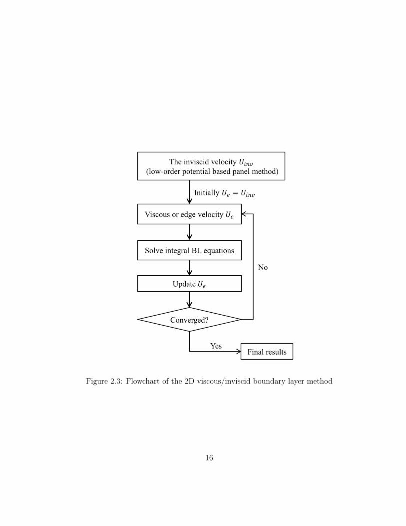
2.3 Flowchart of the 2D viscous/inviscid boundary layer method . 16
2.4 Pressure distributions along the hydrofoil subject to a unifor-m inflow with zero angle of attack, predicted by the presentmethod with increasing number of panels, Re = U∞c
υ= 5, 000, 000,
fixed transition points at 0.1 chord length on both pressure andsuction sides, 1% turbulence level. . . . . . . . . . . . . . . . . 18
2.5 Diagram of the original hydrofoil and the reversed one (tmax/c =0.1, fmax/c = 0.02). . . . . . . . . . . . . . . . . . . . . . . . 19
2.6 Pressure distributions along the two reversed hydrofoils subjectto a uniform inflow with zero angle of attack, predicted by thepresent method, Re = U∞c
υ= 5, 000, 000, fixed transition points
at 0.1 chord length on both the pressure and suction sides, 1%turbulence level. . . . . . . . . . . . . . . . . . . . . . . . . . . 20
2.7 Grid details near the leading and trailing edge of the hydrofoilused in RANS (ANSYS/FLUENT) simulations. . . . . . . . . 20
2.8 Pressure coefficients along the hydrofoil subject to a unifor-m inflow with zero angle of attack, predicted by RANS (AN-SYS/FLUENT) using different grids, Re = U∞c
υ= 5, 000, 000. . 21
2.9 y+ along the hydrofoil body subject to a uniform inflow withzero angle of attack, predicted by RANS (ANSYS/FLUENT)using the refined grid a and b, Re = U∞c
υ= 5, 000, 000. . . . . . 22
2.10 Velocity vectors close to the hydrofoil trailing edge in a unifor-m inflow with zero angle of attack, predicted by RANS (AN-SYS/FLUENT), Re = U∞c
υ= 5, 000, 000. . . . . . . . . . . . . 24
2.11 Diagram of the eight selected eight points . . . . . . . . . . . 25
2.12 Velocity profiles at point 2 and 4 on the hydrofoil surface in auniform inflow with zero angle of attack, predicted by RANS(ANSYS/FLUENT), Re = U∞c
υ= 5, 000, 000. . . . . . . . . . . 25
xiii

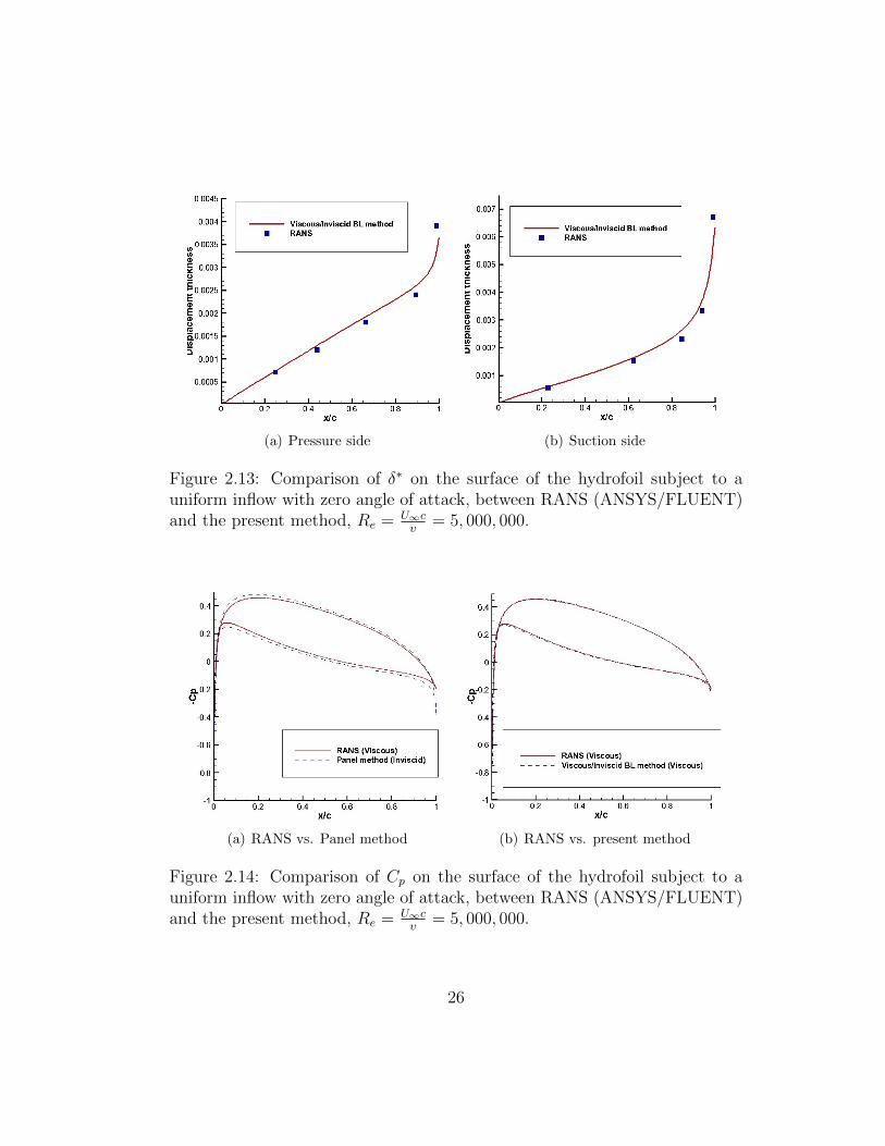
2.13 Comparison of δ∗ on the surface of the hydrofoil subject to auniform inflow with zero angle of attack, between RANS (AN-SYS/FLUENT) and the present method, Re = U∞c
υ= 5, 000, 000. 26
2.14 Comparison of Cp on the surface of the hydrofoil subject to auniform inflow with zero angle of attack, between RANS (AN-SYS/FLUENT) and the present method, Re = U∞c
υ= 5, 000, 000. 26
2.15 Comparison of Cf on the surface of the hydrofoil subject to auniform inflow with zero angle of attack, between RANS (AN-SYS/FLUENT) and the present method, Re = U∞c
υ= 5, 000, 000. 27
3.1 Blade geometry of Propeller NSRDC4381 . . . . . . . . . . . . 30
3.2 Velocity components in t and s directions at the middle chordof the strip r/R = 0.6, of propeller 4381, predicted by RANS(ANSYS/FLUENT), Js = 0.889. . . . . . . . . . . . . . . . . . 31
3.3 Velocity components in t and s directions at the end chord(close to trailing edge) of the strip r/R = 0.6, of propeller 4381,predicted by RANS (ANSYS/FLUENT), Js = 0.889. . . . . . 31
3.4 Velocity components in t and s directions at the middle chordof the strip r/R = 0.95, of propeller 4381, predicted by RANS(ANSYS/FLUENT), Js = 0.889. . . . . . . . . . . . . . . . . . 32
3.5 Velocity components in t and s directions at the end chord(close to trailing edge) of the strip r/R = 0.95, of propeller4381, predicted by RANS (ANSYS/FLUENT), Js = 0.889. . . 32
3.6 Velocity components in t and s directions at the middle chordof the strip r/R = 0.6, of propeller 4381, predicted by RANS(ANSYS/FLUENT), Js = 0.5. . . . . . . . . . . . . . . . . . . 33
3.7 Velocity components in t and s directions at the end chord(close to trailing edge) of the strip r/R = 0.6, of propeller 4381,predicted by RANS (ANSYS/FLUENT), Js = 0.5. . . . . . . . 33
3.8 Velocity components in t and s directions at the middle chordof the strip r/R = 0.95, of propeller 4381, predicted by RANS(ANSYS/FLUENT), Js = 0.5. . . . . . . . . . . . . . . . . . . 34
3.9 Velocity components in t and s directions at the end chord(close to trailing edge) of the strip r/R = 0.95, of propeller4381, predicted by RANS (ANSYS/FLUENT), Js = 0.5. . . . 34
3.10 Sketch of 3D blade paneling . . . . . . . . . . . . . . . . . . . 36
3.11 Flowchart of the iterative scheme for 3D viscous/inviscid bound-ary layer method . . . . . . . . . . . . . . . . . . . . . . . . . 38
xiv

3.12 Pressure distributions along two different strips, r/R=0.6 andr/R=0.9, of Propeller NSTDC 4381, predicted by the presentmethod with and without the effects of blowing sources addedon neighboring blades, Js = 0.889, Re = U∞D
υ= 7.42e5, 1%
turbulence level, fixed transition points at 0.1 chord length onboth the pressure and suction sides of each strip. . . . . . . . 40
3.13 Paneled geometry of Propeller DTMB4119 . . . . . . . . . . . 41
3.14 Pressure distributions predicted by the present method usingdifferent numbers of panels along the strip r/R = 0.62 of Pro-peller DTMB4119, Js = 0.833, Re = U∞D
υ= 766, 395, 1% tur-
bulence level, fixed transition points at 0.1 chord length on boththe pressure and suction sides of each strip. . . . . . . . . . . 42
3.15 Pressure distributions at different iterations on the strip r/R =0.62 of Propeller DTMB4119, predicted by the present method,Js = 0.833, Re = U∞D
υ= 766, 395, 1% turbulence level, fixed
transition points at 0.1 chord length on both the pressure andsuction sides of each strip. . . . . . . . . . . . . . . . . . . . . 43
3.16 Comparison of displacement thickness on the pressure side ofthe strip r/R = 0.7 of Propeller DTMB4119 between exper-iments and the present method (free transition point on thepressure side of each strip, 1% turbulence level), Js = 0.833,Re = U∞D
υ= 766, 395. . . . . . . . . . . . . . . . . . . . . . . . 44
3.17 Comparison of displacement thickness on the suction side of thestrip r/R = 0.7 of Propeller DTMB4119 between experimentsand the present method (fixed transition point at 0.5 chordlength on the suction side of each strip, 1% turbulence level),Js = 0.833, Re = U∞D
υ= 766, 395. . . . . . . . . . . . . . . . . 44
3.18 Comparison of pressure coefficients on the strip, r/R = 0.3 of,of Propeller DTMB4119 between experiments and the presentmethod (fixed transition point at 0.5 chord length on the suctionside and free transition point on the pressure side of each strip,1% turbulence level), Js = 0.833, Re = U∞D
υ= 766, 395. . . . . 45
3.19 Comparison of pressure coefficients on the strip, r/R = 0.7 of,of Propeller DTMB4119 between experiments and the presentmethod (fixed transition point at 0.5 chord length on the suctionside and free transition point on the pressure side of each strip,1% turbulence level), Js = 0.833, Re = U∞D
υ= 766, 395. . . . . 46
xv

3.20 Comparison of pressure coefficients on the strip, r/R = 0.9 of,of Propeller DTMB4119 between experiments and the presentmethod (fixed transition point at 0.5 chord length on the suctionside and free transition point on the pressure side of each strip,1% turbulence level), Js = 0.833, Re = U∞D
υ= 766, 395. . . . . 47
3.21 Comparisons of KT and KQ of Propeller DTMB4119 at differentadvance ratios, between experiments and the present method. 49
3.22 Paneled geometry of Propeller NSRDC4381. . . . . . . . . . . 50
3.23 Domain and boundary conditions of the RANS (ANSYS/FLUENT)case for Propeller NSRDC4381 (from Sharma 2011). . . . . . . 51
3.24 Grid details used in the RANS (ANSYS/FLUENT) case forPropeller NSRDC4381. Top left: O type grid on the propellerblade. Top right: grid details on the hub around the root sectionof the propeller blade. Bottom left: Grid details on the hub nearthe leading edge of the root section of propeller blade. Bottomright: grid details on the hub near the trailing edge of the rootsection of the propeller blade. (from Sharma 2011). . . . . . . 52
3.25 Pressure distributions predicted by the present method usingdifferent numbers of panels at strips, r/R = 0.6 and r/R = 0.9,of Propeller NSRDC4381, Js = 0.889, Re = U∞D
υ= 7.42e5, 1%
turbulence level, fixed transition points at 0.1 chord length onboth the pressure and suction sides of each strip. . . . . . . . 53
3.26 Pressure distributions at different iterations at strips r/R = 0.6and r/R = 0.9 of Propeller NSRDC4381, predicted by thepresent method, Js = 0.889, Re = U∞D
υ= 7.42e5, 1% turbu-
lence level, fixed transition points at 0.1 chord length on boththe pressure and suction sides of each strip. . . . . . . . . . . 54
3.27 Comparison of pressure distributions along the strip, r/R = 0.6,of Propeller NSRDC4381, predicted by RANS (ANSYS/FLUENT),panel method and the present method (fixed transition points at0.1 chord length on both the pressure and suction sides of eachstrip, 1% turbulence level), Js = 0.889, Re = U∞D
υ= 7.42e5 for
viscous cases. . . . . . . . . . . . . . . . . . . . . . . . . . . . 55
3.28 Comparison of pressure distributions along the strip, r/R = 0.8,of Propeller NSRDC4381, predicted by RANS (ANSYS/FLUENT),panel method and the present method (fixed transition points at0.1 chord length on both the pressure and suction sides of eachstrip, 1% turbulence level), Js = 0.889, Re = U∞D
υ= 7.42e5 for
viscous cases. . . . . . . . . . . . . . . . . . . . . . . . . . . . 56
xvi

3.29 Comparison of pressure distributions along the strip, r/R = 0.6,of Propeller NSRDC4381, predicted by RANS (ANSYS/FLUENT),panel method and the present method (fixed transition pointsat 0.1 chord length on both the pressure and suction sides ofeach strip, 1% turbulence level), Js = 0.5, Re = U∞D
υ= 4.15e5
for viscous cases. . . . . . . . . . . . . . . . . . . . . . . . . . 57
3.30 Comparison of pressure distributions along the strip, r/R = 0.8,of Propeller NSRDC4381, predicted by RANS (ANSYS/FLUENT),panel method and the present method (fixed transition pointsat 0.1 chord length on both the pressure and suction sides ofeach strip, 1% turbulence level), Js = 0.5, Re = U∞D
υ= 4.15e5
for viscous cases. . . . . . . . . . . . . . . . . . . . . . . . . . 58
3.31 Comparison of Cf at strips, r/R = 0.6 and r/R = 0.6, of Pro-peller NSRDC4381, between RANS (ANSYS/FLUENT) andthe present method (fixed transition points at 0.1 chord lengthon both the pressure and suction sides of each strip, 1% turbu-lence level), Js = 0.889, Re = U∞D
υ= 7.42e5. . . . . . . . . . . 59
3.32 Comparisons of KT and KQ of Propeller NSRDC4381 at differ-ent advance ratios, between the present method combined withPSF2 wake alignment and experiments. . . . . . . . . . . . . . 60
3.33 Comparisons of KT and KQ of Propeller NSRDC4381 at differ-ent advance ratios, between the present method combined withfull wake alignment and experiments. . . . . . . . . . . . . . . 61
3.34 Paneled geometry of the DTMB Duct II. . . . . . . . . . . . . 62
3.35 Pressure distributions on DTMB Duct II predicted by the presentmethod using different numbers of panels on both the chordand span wise directions, Re = U∞D
υ= 2.06e6, fixed transition
points at 0.05 chord length on both the pressure and suctionsides of each strip, 1% turbulence level. . . . . . . . . . . . . . 63
3.36 Pressure distributions at different iterations on DTMB Duct II,predicted by the present method, Re = U∞D
υ= 2.06e6, fixed
transition points at 0.05 chord length on both the pressure andsuction sides of each strip, 1% turbulence level. . . . . . . . . 64
3.37 Pressure distributions along three different sections of DTMBDuct II, predicted by the present method, Re = U∞D
υ= 2.06e6,
fixed transition points at 0.05 chord length on both the pressureand suction sides of each strip, 1% turbulence level. . . . . . . 65
xvii

3.38 Displacement thickness of boundary layer along three differen-t sections of DTMB Duct II, predicted by the present method,Re = U∞D
υ= 2.06e6, fixed transition points at 0.05 chord length
on both the pressure and suction sides of each strip, 1% turbu-lence level. . . . . . . . . . . . . . . . . . . . . . . . . . . . . . 66
3.39 Viscous and inviscid pressure distributions on the DTMB DuctII predicted by the present method (fixed transition points at0.05 chord length on both the pressure and suction sides of eachstrip, 1% turbulence level), compared with the experimentalmeasurements by Morgan and Caster (1965), Re = U∞D
υ= 2.06e6. 67
4.1 Diagram of a straight wing blade adjacent to a slip wall . . . 69
4.2 Diagram of a straight wing blade and its images, symmetricabout the red line . . . . . . . . . . . . . . . . . . . . . . . . . 69
4.3 Diagram of the equivalence of the influence coefficients, fromSingh (2009) . . . . . . . . . . . . . . . . . . . . . . . . . . . . 71
4.4 Diagram of a wing blade between two parallel walls . . . . . . 72
4.5 Pressure distributions along the strip at r/R = 0.75, predictedby the present method using different numbers of panels on spanand chord wise directions, Re = U∞c
υ= 1.0e6, fixed transition
points at 0.1 chord length on both the pressure and suction sidesof each strip, 1% turbulence level. . . . . . . . . . . . . . . . 73
4.6 Circulations on the straight wing blade predicted by the originalimage model of Singh (2009) using different numbers of images. 74
4.7 Pressure distributions along the strip at r/R = 0.6 of the s-traight wing blase, predicted by the original and the presentimage model, using different numbers of images. For the vis-cous case, Re = U∞c
υ= 1.0e6, fixed transition points at 0.1 chord
length on both the pressure and suction sides of each strip, 1%turbulence level. . . . . . . . . . . . . . . . . . . . . . . . . . 75
4.8 Pressure distributions on the strips at r/R = 0.3, r/R = 0.5 andr/R = 0.9 of the straight wing blade, predicted by the originaland the present image model, using different numbers of images.For the viscous case, Re = U∞c
υ= 1.0e6, fixed transition points
at 0.1 chord length on both the pressure and suction sides ofeach strip, 1% turbulence level. . . . . . . . . . . . . . . . . . 76
4.9 Diagram of the domain of the straight wing blade between twoparallel slip walls for 3D RANS (ANSYS/FLUENT) simulations. 77
4.10 Grid details around the straight wing blade used in 3D RANS(ANSYS/FLUENT) simulations. . . . . . . . . . . . . . . . . 78
xviii

4.11 Pressure coefficients on the strips at r/R=0.2 and r/R=0.6 ofthe 3D straight wing predicted by the 3D RANS (ANSYS/FLUENT)case, and on the 2D strip predicted by the 2D RANS (AN-SYS/FLUENT) case, Re = U∞c
υ= 1.0e6. . . . . . . . . . . . . 79
4.12 Pressure coefficients along the strip at r/R=0.5 of the 3D s-traight wing predicted by RANS (ANSYS/FLUENT), the presentmethod (fixed transition points at 0.1 chord length on both thepressure and suction sides of each strip, 1% turbulence level)and the panel method. For the viscous case, Re = U∞c
υ= 1.0e6. 80
4.13 Diagram of a swept wing between two parallel slip walls. . . . 82
4.14 Pressure distributions on the strips at r/R = 0.3, r/R = 0.5 andr/R = 0.9 of the wing blade, predicted by the present method,Re = U∞c
υ= 1.0e6, fixed transition points at 0.1 chord length on
both the pressure and suction sides of each strip, 1% turbulencelevel. . . . . . . . . . . . . . . . . . . . . . . . . . . . . . . . . 82
4.15 Pressure coefficients on the strip at r/R=0.025 of the 3D sweptwing, predicted by the 3D RANS (ANSYS/FLUENT) case, thepresent method (fixed transition points at 0.1 chord length onboth the pressure and suction sides of each strip, 1% turbulencelevel) and the panel method. For the viscous case, Re = U∞c
υ=
1.0e6. . . . . . . . . . . . . . . . . . . . . . . . . . . . . . . . 83
4.16 Pressure coefficients on the strip at r/R=0.5 of the 3D sweptwing, predicted by the 3D RANS (ANSYS/FLUENT) case, thepresent method (fixed transition points at 0.1 chord length onboth the pressure and suction sides of each strip, 1% turbulencelevel) and the panel method. For the viscous case, Re = U∞c
υ=
1.0e6. . . . . . . . . . . . . . . . . . . . . . . . . . . . . . . . 84
4.17 Pressure coefficients on the strip at r/R=0.975 of the 3D sweptwing, predicted by the 3D RANS (ANSYS/FLUENT) case, thepresent method (fixed transition points at 0.1 chord length onboth the pressure and suction sides of each strip, 1% turbulencelevel) and the panel method. For the viscous case, Re = U∞c
υ=
1.0e6. . . . . . . . . . . . . . . . . . . . . . . . . . . . . . . . 85
5.1 Section with a non-zero thickness trailing edge, extracted fromthe ONR-AxWj-2 rotor blade . . . . . . . . . . . . . . . . . . 87
5.2 Diagram of the modification of the trailing edge with non-zerothickness . . . . . . . . . . . . . . . . . . . . . . . . . . . . . 88
5.3 Diagram of the extension after the open trailing edge, from Pan(2009) . . . . . . . . . . . . . . . . . . . . . . . . . . . . . . . 88
xix

5.4 Diagram of extension of the trailing edge with non-zero thickness 90
5.5 Diagram of the procedure of the search scheme for extension . 91
5.6 Comparison of pressure distributions on the strip extracted fromthe ONR-AxWJ-2 rotor blade at r/R = 0.7, between RANS(ANSYS/FLUENT) and the present method (fixed transitionpoints at 0.01 chord length on both the pressure and suctionsides, 1% turbulence level), Re = U∞c
υ= 5.0e6. . . . . . . . . 92
5.7 Final extension behind the the strip extracted from the ONR-AxWJ-2 rotor blade at r/R = 0.7, predicted by the presentmethod, Re = U∞c
υ= 5.0e6, fixed transition points at 0.01 chord
length on both the pressure and suction sides, 1% turbulencelevel. . . . . . . . . . . . . . . . . . . . . . . . . . . . . . . . . 93
5.8 Pressure difference ∆p of the cut points vs. vertical position ofthe last camber point yC , of the ONR-AxWJ-2 rotor blade atr/R = 0.7, from the present method, Re = U∞c
υ= 5.0e6, fixed
transition points at 0.01 chord length on both the pressure andsuction sides, 1% turbulence level. . . . . . . . . . . . . . . . . 94
5.9 Comparison of pressure distributions along the NACA hydrofoilwith a non-zero thickness trailing edge, between RANS (AN-SYS/FLUENT) and the present method (fixed transition pointsat 0.01 chord length on both the pressure and suction sides, 1%turbulence level), Re = U∞c
υ= 9.0e6. . . . . . . . . . . . . . . 95
5.10 Final extension behind the NACA hydrofoil with a non-zerothickness trailing edge, predicted by the present method, Re =U∞cυ
= 5.0e6, fixed transition points at 0.01 chord length onboth the pressure and suction sides, 1% turbulence level. . . . 96
5.11 Pressure difference ∆p of the cut points vs. vertical position ofthe last camber point yC , of the NACA hydrofoil with a non-zerothickness trailing edge, from the present method, Re = U∞c
υ=
5.0e6, fixed transition points at 0.01 chord length on both thepressure and suction sides, 1% turbulence level. . . . . . . . . 97
5.12 Propeller with non-zero trailing edge thickness, from Pan (2009). 99
5.13 Propeller with closed sharp trailing edge modified by the presentscheme. . . . . . . . . . . . . . . . . . . . . . . . . . . . . . . 100
5.14 Pressure differences between the cut points of strip 1 and neigh-boring strips vs. the movement of the last camber point of strip1. . . . . . . . . . . . . . . . . . . . . . . . . . . . . . . . . . . 101
5.15 Pressure differences between the cut points of strip 5 and neigh-boring strips vs. the movement of the last camber point of strip5. . . . . . . . . . . . . . . . . . . . . . . . . . . . . . . . . . . 101
xx

5.16 Pressure differences between the cut points of strip 10 andneighboring strips vs. the movement of the last camber pointof strip 10. . . . . . . . . . . . . . . . . . . . . . . . . . . . . . 102
5.17 Pressure differences between the cut points of strip 18 andneighboring strips vs. the movement of the last camber pointof strip 18. . . . . . . . . . . . . . . . . . . . . . . . . . . . . . 102
5.18 Pressure differences between the cut points on the initial andfinal extensions. . . . . . . . . . . . . . . . . . . . . . . . . . . 104
5.19 Circulation on the final blade geometry. . . . . . . . . . . . . . 104
5.20 KT of the propeller with finite thickness trailing edge. . . . . . 105
5.21 KQ of the propeller with finite thickness trailing edge. . . . . . 106
xxi

Nomenclature
Latin Symbols
Cτ shear stress coefficient Cτ = τmax/(ρU2)
Cf skin-friction coefficient Cf = τwall/(0.5ρU2)
Cp pressure coefficient, Cp = (P − Po)/(0.5ρn2D2)
D propeller diameter, D = 2R
D dissipation or shear work integral, D =∫ δ0
(τ1
∂u∂x3
+ τ2∂w∂x3
)dx3
fmax/C maximum camber to chord ratio
G Green’s function
H shape factor, H = δ∗/θ
H∗ kinetic energy shape factor, θ∗/θ
J advance ratio based on Vs, J = Vs/(nD)
KQ torque coefficient, KQ = Q/(ρn2D5)
KT thrust coefficient, KT = T/(ρn2D4)
xxii

q total velocity
Q torque
U in local inflow velocity (in the propeller fixed system)
u Perturbation velocity
qe Magnitude of edge velocity
R propeller radius
Re Reynolds number
SP blade surface
SW wake surface
K thrust
tmax/C maximum thickness to chord ratio
ue boundary layer edge velocity
uτ wall shear velocity, uτ =√τwall/ρ
x, y, z propeller fixed coordinates
y+ non-dimensional wall distance, y+ = uτyν
xxiii

Greek Symbols
α angle of attack
δ∗ displacement thickness, δ∗ =∫
(1− uUe
)dz
∆t time step size
ω propeller angular velocity
ν kinematic viscosity of water
φ perturbation potential
Φ total potential
ρ fluid density
θ momentum thickness, θ =∫
uUe
(1− uUe
)dz
θ∗ kinetic energy thickness, θ∗ =∫
uUe
(1− u2
U2e)dz
Uppercase Abbreviations
2D two dimensional
3D three dimensional
CPU central processing unit
MIT Massachusetts Institute of Technology
NACA National Advisory Committee for Aeronautics
RANS Reynolds-averaged Navier Stokes
xxiv

Computer Program Names
CAV2DBL cavitating 2-dimensional with boundary layer
Fluent A commercial RANS solver
PROPCAV cavitating propeller potential flow solver based on BEM
XFOIL 2D integral boundary layer analysis code
xxv

Chapter 1
Introduction
1.1 Background
Panel methods have been extensively used in the design stage of ma-
rine propellers due to the satisfactory prediction of propeller performance with
small computational cost. However, since they are based on the inviscid po-
tential flow theory, classical panel methods cannot predict the effects of fluid
viscosity. For propeller flows, viscosity can not only cause friction but also af-
fect the pressure on propeller blades, resulting in the changes of thrust/torque
forces and propeller efficiency. Some empirical methods can be used with pan-
el methods to take account of the effects of fluid viscosity. Kerwin and Lee
(1978) used an adopted constant as the skin friction coefficient to include the
contribution of the viscous shear stress and an empirical viscous pitch cor-
rection to approximate the influences of the boundary layer. However, such
empirical methods require user adjustable constants, which could be good for
some cases, but inaccurate for some other cases. In order to handle the effect-
s of viscosity for general blade geometries and various flow conditions, more
rational methods are required.
Viscous/inviscid interactive methods in 2D have been highly developed
1

in the past decades, from which the fully simultaneous coupling scheme devel-
oped by Drela (1985, 1987) has been proved to be the most robust and efficient
one for 2-D separated flows. Drela (1989) implemented a viscous/inviscid in-
teractive solver, XFOIL, for 2D airfoils. XFOIL uses the stream function to
get the inviscid flow field. Then the inviscid solution is coupled with the 2D in-
tegral boundary layer equations to solve for the boundary layer variables. The
development of the viscous/inviscid interactive methods in 3D is limited be-
cause of the complexity of 3D boundary layer. Cousteix and Houdeville (1981)
pointed out that the 3D integral boundary layer equations consist of three fully
hyperbolic non-linear partial differential equations. Milewski (1997) develope-
d a 3D fully simultaneous viscous/inviscid interactive scheme, by coupling a
potential based panel method and the 3D integral boundary layer equation-
s, for 3D wetted hydrofoil and duct flows. However, such a scheme requires
a large amount of computer resources and is very difficult to be applied to
complicated geometries such as propeller blades. For 3D propeller cases par-
ticularly, Jessup (1989) measured the boundary layer variables on the blades
of Propeller DTMB 4119 and found that the boundary layer variables on the
stream wise direction are much more significant than those on the span wise
direction. According to Jessup’s measurements, Hufford (1992, 1994) assumed
that the effects of the boundary layer on propeller blades should be negligible
radially outward compared with those along constant radius. Based on the
above assumption, he proposed a method used to predict the 3D boundary
layer effects on propeller blades. His method calculates the inviscid solution
2

by a potential based panel method and then applies a 2D viscous/inviscid
interactive method to each strip along constant radius of the blades using,
however, 3D boundary layer sources over each strip. Sun (2008) coupled a
potential based panel method code, PROPCAV, with XFOIL following Huf-
ford’s method, but further simplified the method by adding 2D boundary layer
sources over the strips. However, Hufford and Sun considered the boundary
layer on each strip independently and ignored the boundary layer effects of
neighboring strips and other blades, which oversimplified the problem.
1.2 Objective
The main objective of this thesis is to develop a more reasonable and
complete 3D viscous/inviscid interactive method by coupling a 3D low-order
potential based panel method code, PROPCAV, with Drela’s 2D integral
boundary layer solver, XFOIL, to investigate the effects of fluid viscosity on
the performance of propellers.
1.3 Organization
This thesis is organized into six chapters.
Chapter 1 contains the literature review, the objective and the organi-
zation of this study.
Chapter 2 introduces a two-dimensional viscous/inviscid interactive
method in details. This method is applied to a 2D hydrofoil case, and the
3

results are correlated with RANS (ANSYS/FLUENT) results.
Chapter 3 develops a three dimensional viscous/inviscid interactive
method for propeller and duct flows. The method follows the assumption
of Hufford (1992, 1994) and Sun (2008) that the boundary layer along the
span wise direction (radially outward for propeller blades) can be negligible,
but further considers the boundary layer effects from neighboring strips and
blades. Then this method is validated through two propeller and a bare duct
cases.
Chapter 4 extends the three dimensional viscous/inviscid interactive
method to an image model used to consider the effects of slip walls. Cases of
a straight and a swept wing blade between two parallel walls are carried out
to validate the image model.
Chapter 5 improves the scheme proposed by Pan (2009, 2011) for hydro-
foils and propeller blades with non-zero thickness trailing edges. The results
of sample cases are presented.
Chapter 6 summarizes the work of this thesis and presents the recom-
mendations for future research.
4

Chapter 2
Two Dimensional Viscous/Inviscid Interactive
Method
In this chapter, a 2D viscous/inviscid interactive method is introduced.
This method couples a 2D low-order potential based panel method and the 2D
integral boundary layer analysis. The chapter starts with the introduction of
the 2D wall transpiration model and then derives the expression of the viscous
or edge velocity. In the following, the 2D integral boundary layer equations are
summarized. The coupling algorithm between the invsicid and viscous solution
is presented next. Finally, this method is applied to a 2D hydrofoil case. The
results are compared with those predicted by RANS (ANSYS/FLUENT).
2.1 Governing Equations
A lower-order panel method, in which constant sources and dipoles
are used, based on perturbation potential is applied in this thesis. The to-
tal velocity is decomposed into two components: the inflow velocity and the
perturbation velocity.
q = U in + u (2.1)
5

where q is the total velocity, Uin is the velocity of incoming flow, and u is the
perturbation velocity.
u = ∇φ (2.2)
q = ∇Φtotal (2.3)
The perturbation potential φ satisfies the Laplace Equation:
∇2φ = 0 (2.4)
The Laplace Equation can be integrated on the boundaries:
φp2
=
∫∫Sp
[−φp′
∂G(p, p′)
∂np′+∂φp′
∂np′G(p, p′)
]dS
−∫∫
SW
∆φw(p′)∂G(p, p′)
∂np′dS
(2.5)
where p and p′ correspond to the field point and the variable point; G(p, p′) =
− 14πr
for three dimension or G(p, p′) = ln(r)2π
for two dimension, is the Green’s
function with r being the distance between the field point p and the variable
point p′; ∆φw is the potential jump across the wake; SP and SW represent the
blade surface and wake sheet, respectively.
2.2 Boundary Conditions
In order to obtain an unique solution of (2.5), appropriate boundary
conditions are applied to the flow domain. For fully wetted cases, the kinematic
boundary condition states:
∂φ
∂n= −U in · n (2.6)
6

where n is the normal vector on the blade surface pointing into the flow field.
At the trailing edge of the blade, Kutta condition is applied, which implies the
finite velocity at the blade trailing edge.
∇φ = finite (2.7)
At the far field, the perturbation velocity vanishes.
∇φ = 0 (2.8)
2.3 2D Wall Transpiration Model
A 2D wall transpiration model is introduced in this section to simulate
the 2D viscous boundary layer. This model couples the potential and the
2D integral boundary layer equations through the edge velocity. The detailed
derivation of the expression of the edge or viscous velocity is presented.
2.3.1 Boundary Layer Simulation
For the potential flow, blowing sources are added on the wall to simulate
the boundary layer in the real viscous flow (shown in Fig. 2.1). The blowing
sources should be given proper strengthes so that the velocity at the edge
of boundary layer, y = ye, is the same with that in the real viscous flow.
According to the Bernoulli equation, the same edge velocities in the two flows
lead to the same pressures on y = ye. In addition, the boundary layer theory
tells that the pressure cross the boundary layer stays constant, which means
that the pressures on the point A of the edge of boundary layer and point B
7

of the wall are the same. Thus it is concluded that the pressure on the wall
in the equivalent inviscid flow is the same with that in the real viscous flow.
So far, the effects of the boundary layer on the pressure have been considered
in the equivalent inviscid flow by adding proper blowing sources on the wall.
In addition, the friction on the wall can be considered by solving the integral
boundary layer equations.
𝑦 = 𝑦𝑒
A
B
(a) Real viscous flow
𝑦 = 𝑦𝑒
Induced normal velocity by the sources
A’
(b) Equivalent inviscid flow
Figure 2.1: Velocity profiles for the real viscous and equivalent inviscid flow
2.3.2 Edge Velocity Expression
The expression of the edge velocity Ue or viscous velocity Uvis for 2D
hydrofoil cases are derived in this subsection. For 2D hydrofoil cases (shown
in Fig. 2.2), (2.5) becomes:
πφp =
∫Sp
(∂φ
∂nln r − φ∂ ln r
∂n
)ds−
∫SW
(∆φw
∂ ln r
∂n+
)ds (2.9)
8

where φp is the perturbation potential on the hydrofoil body. The discretized
expression of (2.9) is
N∑j=1
Dijφj =N∑j=1
Sij
(∂φ
∂n
)j
−Wi∆φw (2.10)
The Kutta condition can be satisfied using a modified Morino Kutta condition
proposed by Kinnas et al. (1990)
∆φ = ΦN − Φ1 + U in · rt (2.11)
where rt is the distance between the control points of the upper and lower
trailing edge panels (the 1st and the N th panel). Then (2.10) becomes:
N∑j=1
Aijφj =N∑j=1
Sij
(∂φ
∂n
)j
−Wi (U in · rt) (2.12)
(2.12) can be used to calculate the perturbation potential on the hydrofoil. To
consider the effects of fluid viscosity, blowing sources with unknown strength
are added on both the body and the wake panels to simulate viscous boundary
layer. When the added blowing sources are taken into consideration, (2.12)
𝑼𝒊𝒏
n
𝒏+
Figure 2.2: The diagram of the paneling on a 2D hydrofoil and its wake
9

becomes:
N∑j=1
Aijφj =N∑j=1
Sij
(∂φ
∂n
)j
−Wi (U in · rt) +
N+NW∑j=1
Bijσj (2.13)
where σj is the unknown strength of the blowing source added at the panel
j; Bij is the source induced influence coefficient analogous to Sij; N and NW
indicate the number of panels on the hydrofoil body and the wake, respectively.
Then the perturbation potential on the body panel can be obtained from
(2.13):
φi =N∑j=1
A−1ij
[N∑j=1
Sjk
(∂φ
∂n
)k
−Wi (U in · rt)
]
+
N+NW∑j=1
(N∑j=1
A−1ik Bkj
)σj
(2.14)
(2.14) is the expression of the perturbation potential taken the added blowing
sources into consideration, or it can be called the viscous perturbation poten-
tial. The total potential for viscous cases should be the sum of the viscous
perturbation potential and the inflow potential:
Φi,vis = Φini + φi,vis
= Φini +
N∑j=1
A−1ij
[N∑j=1
Sjk
(∂φ
∂n
)k
−Wi (U in · rin)
]+
N+NW∑j=1
(N∑j=1
A−1ij Bkj
)σj
= Φini + φi,inv +
N+NW∑j=1
Hijσj
= Φi,inv +
N+NW∑j=1
Hijσj
(2.15)
10

where Hij =∑N
j=1A−1ij Bkj. According to (2.15), the total viscous potential
Φi,ivs consists of the total inviscid potential Φi,inv and the induced potential
by the added blowing sources∑N+NW
j=1 Hijσj. The viscous velocity or edge
velocity can be obtained by differentiating the total viscous potential along
the surface of the hydrofoil:
Ui,vis =∂Φi,ivs
∂s
=∂Φi,inv
∂s+
∂
∂s
(N+NW∑j=1
Hijσj
)
= Ui,inv +
N+NW∑j=1
Cijσj
(2.16)
The viscous velocity on the hydrofoil body can be expressed as (2.16). The
derivative of Hij can be achieved by:
Cij =∂Hij
∂s=Hi,j −Hi−1,j
∆s(2.17)
(2.16) states that the viscous velocity Ui,vis is the sum of the inviscid velocity
Ui,inv and the induced velocity by the added blowing sources∑N+NW
j=1 Cijσj.
It should be noted that the inflow potential Φin does not exist in the cases
with rotational inflows. Even though the derivation of (2.16) uses the inflow
potential Φin, (2.16) is still general and valid for cases with or without the
inflow potential. This is because (2.16) is an expression in terms of velocity
instead of potential.
The viscous velocity on the wake sheet can be derived similarly. With
the added blowing sources, the perturbation potential (viscous perturbation
11

potential) on the wake can be written as
φwake =1
2π
∫SP
(∂φ
∂nln r − φ∂ ln r
∂n
)ds+
1
2π
∫SP+SW
(ln r)σds (2.18)
Discretizing (2.18) gives:
φwakei =N∑j=1
Awijφj +N∑j=1
Cwij
(∂φ
∂n
)j
+
N+NW∑j=1
Bwijσj (2.19)
where Awij, Cwij and Bw
ij are the influence coefficients analogues to those in (2.13)
for hydrofoil body. φj in (2.19) is the viscous perturbation potential on the
panel j of the hydrofoil body, which is the sum of the inviscid perturbation
potential and the induced potential due to the blowing sources:
φj = φj,inv +
N+NW∑j=1
Hjkσk (2.20)
Replace φj in (2.19) with (2.20) and gives:
φwakei =N∑j=1
Awij
[φinvj +
N+NW∑j=1
Hjkσk
]+
N∑j=1
Cwij
(∂φ
∂n
)j
+
N+NW∑j=1
Bwijσj
=N∑j=1
Awijφj,inv +N∑j=1
Cwij
(∂φ
∂n
)j
+
N+NW∑j=1
(N∑k=1
AwjkHkj +Bwij
)σj
= φwakei,inv +
N+NW∑j=1
Hwijσj
(2.21)
The viscous total potential should be:
Φwakei,vis = Φin
i + φwakei,vis
= Φini + φwakei,inv +
N+NW∑j=1
Hwijσj
= Φwakei,inv +
N+NW∑j=1
Hwijσj
(2.22)
12

Then the viscous or edge velocity can be written as:
Uwakei,ivs =
∂Φwakei,vis
∂s
=∂Φwake
i,inv
∂s+
∂
∂s
(N+NW∑j=1
Hwijσj
)
= Uwakei,inv +
N+NW∑j=1
Cwijσj
(2.23)
(2.16) and (2.23) express the viscous velocity on the hydrofoil body and wake
using the inviscid velocity, which can be solved by the low-order potential
based panel method, and the induced velocity by the added blowing sources.
The viscous velocity on the body and wake can be written in a general form:
Ui,vis = Ui,inv +
N+NW∑j=1
Gijσj (2.24)
where Gij = Cij on the hydrofoil body and Gij = Cwij on the wake. i is from
1 to N +NW . The unknown strength of the blowing source is directly related
to the boundary layer values by:
σ =∂ (Uvisδ
∗)
∂s=∂m
∂s(2.25)
where δ∗ is the displacement thickness of boundary layer, and m = Uvisδ∗ is
defined as the mass defect. (2.25) can be calculated numerically
σj =mj+1 −mj
∆s(2.26)
By replacing the blowing source strength σj in (2.24) with (2.26), the final
expression for viscous velocity is obtained:
Ui,vis = Ui,inv +
N+NW∑j=1
Dijmj (2.27)
13

where
Di,j =Gi,j−1
sj − sj−1− Gi,j
sj+1 − sj(2.28)
2.4 The Viscous/Inviscid Flow Coupling
(2.27) needs to be combined with the 2D integral boundary layer equa-
tions. Then the combined equations can be solved together.
2.4.1 2D Integral Boundary Layer Equations
The 2D integral boundary layer equations include the standard integral
momentum and the kinetic energy equation. A closure equation is used to close
the system. For incompressible flow, the 2D integral boundary layer equations
can be expressed as the followings:
• Momentum equation
∂θ
∂s+ (2 +H)
θ
Ue
dUeds
=Cf2
(2.29)
• Kinetic energy equation
θdH∗
ds+H∗(1−H)
θ
Ue
dUeds
= 2CD −H∗Cf2
(2.30)
14

• Closure
Closure for turbulent flows
δ
Cτ
dCτds
= 5.6[C
12τEQ − C
12τ
]+ 2δ
{4
3δ∗
[Cf2−(Hk − 1
6.7Hk
)2]− 1
Ue
dUeds
} (2.31)
Closure for laminar flows
dn
ds=dn(Hk)
dReθ
Reθ(Hk, θ)
ds(2.32)
2.4.2 Coupling Algorithm
The brief solution procedures of this viscous/inviscid interactive method
includes the following steps (as shown in Fig. 2.3): First, the inviscid velocity
Uinv is calculated by the low-order potential based panel method. Then the
viscous or the edge velocity Uvis is given as the inviscid velocity. The 2D in-
tegral boundary layer equations and the closure can be solved to obtain the
boundary layer variables. Next, the viscous velocity is updated using (2.24).
Repeat this process until a converged result is obtained.
2.5 2D Viscous Hydrofoil Case
A 2D hydrofoil case is carried out in order to validate the 2D vis-
cous/inviscid interactive method and test how this method can capture the
boundary layer characteristics. The hydrofoil is generated based on the NACA00
thickness form with tmax/c = 0.1. A camber with fmax/c = 0.02 is added. It
15
The inviscid velocity 𝑈𝑖𝑛𝑣
(low-order potential based panel method)
Viscous or edge velocity 𝑈𝑒
Solve integral BL equations
Initially 𝑈𝑒 = 𝑈𝑖𝑛𝑣
Update 𝑈𝑒
Converged?
No
Yes Final results
Figure 2.3: Flowchart of the 2D viscous/inviscid boundary layer method
16

is subject to a uniform inflow with zero angle of attack. The transition points
on both pressure and suction side of the hydrofoil used in the present method
are fixed close to the leading edge. The turbulence level is given as 1%. The
Reynolds number is selected to be 5,000,000. The results predicted by the
2D viscous/inviscid interactive method and RANS (ANSYS/FLUENT) are
compared.
2.5.1 Method Validation
A grid dependency study of the present viscous/inviscid interactive
method is conducted first. The pressure distributions along the hydrofoil pre-
dicted by the present method using different numbers of panels are plotted in
Fig. 2.4. The plots in Fig. 2.4 collapse into the same line, indicating that the
changes of the number of panels on the hydrofoil do not affect the final results.
Another case of a reversed hydrofoil is conducted to validate the present
method. The same NACA hydrofoil is reversed up and down as shown in Fig.
2.5. Subject to the same inflow, the pressure on the reversed hydrofoil is
expected the same with that on the original hydrofoil. Fig. 2.6 plots the
pressure distributions on the two hydrofoils predicted by the present method.
The practically identical curves shown in Fig. 2.6 provide a good verification
test of the present method.
17

Figure 2.4: Pressure distributions along the hydrofoil subject to a uniform in-flow with zero angle of attack, predicted by the present method with increasingnumber of panels, Re = U∞c
υ= 5, 000, 000, fixed transition points at 0.1 chord
length on both pressure and suction sides, 1% turbulence level.
18

2.5.2 Result Comparison with RANS (ANSYS/FLUENT)
A grid dependence study of the RANS case is conducted first. The
RANS simulations are carried out in a rectangular domain. A free stream
condition with a specified velocity is imposed on the left, top and bottom
boundaries. The outflow condition is set at the right boundary as the outlet
of the domain. The grid details around the leading and trailing edge of the
hydrofoil are shown in Fig. 2.7. The grid is refined and the three grids used
in the grid dependency study are listed in Table 2.1. The plots of the pressure
coefficient along the hydrofoil predicted by RANS using these three grids col-
lapse into a same line (shown in Fig. 2.8), indicating that the grids work fine
for this case.
Figure 2.5: Diagram of the original hydrofoil and the reversed one (tmax/c =0.1, fmax/c = 0.02).
19

Figure 2.6: Pressure distributions along the two reversed hydrofoils subject toa uniform inflow with zero angle of attack, predicted by the present method,Re = U∞c
υ= 5, 000, 000, fixed transition points at 0.1 chord length on both the
pressure and suction sides, 1% turbulence level.
(a) Leading edge (b) Trailing edge
Figure 2.7: Grid details near the leading and trailing edge of the hydrofoilused in RANS (ANSYS/FLUENT) simulations.
20

Figure 2.8: Pressure coefficients along the hydrofoil subject to a uniform in-flow with zero angle of attack, predicted by RANS (ANSYS/FLUENT) usingdifferent grids, Re = U∞c
υ= 5, 000, 000.
21

Table 2.1: Three grids used for the grid dependency study of the RANS (AN-SYS/FLUENT) case for 2D hydrofoil
Grid Original Refined a Refined bCell number 45,878 473,822 1,259,924
To ensure sufficient resolution to capture the boundary layer character-
istics, the value of y+ on the hydrofoil surface should be limited to be less than
5. Fig. 2.9 plots y+ on the hydrofoil using the two refined meshes. Either one
of the two meshes is proven to have sufficient resolution. The refined mesh b
is used for the following study. The information for the RANS case is listed
in Table. 2.2.
(a) Refined grid a (b) Refined grid b
Figure 2.9: y+ along the hydrofoil body subject to a uniform inflow with zeroangle of attack, predicted by RANS (ANSYS/FLUENT) using the refined grida and b, Re = U∞c
υ= 5, 000, 000.
The velocity vectors in the flow domain close to the hydrofoil trailing
edge predicted by RANS are shown in Fig. 2.10. No separation happens in
22

Table 2.2: Information of the RANS (ANSYS/FLUENT) case for 2D hydrofoilReynolds number 5, 000, 000Turbulence model k-ω SST
Pressure correction scheme SIMPLECSpatial discretization Second order upwind
Total time for calculate (8 CPUs) 4,386 seconds
this case. Obvious effects of the boundary layer can be observed in the figure.
To analyze the boundary layer quantitatively, the displacement thickness δ∗ is
introduced, which is defined as
δ∗ =
∫ ∞0
(1− u
Ue
)dy (2.33)
Eight points (shown in Fig. 2.11) are selected on the surface of the hydrofoil.
Along the normal direction of each point, the velocity profile can be exported
from the RANS case, and the displacement thickness at this point can be cal-
culated by (2.33). The velocity profiles at point 2 and point 4 exported from
RANS are plotted in Fig. 2.12. It is reasonable that the thicker boundary layer
is observed at point 2, closer to the trailing edge, than 4. The comparison of
the displacement thickness δ∗ predicted by RANS and the 2D viscous/inviscid
interactive method (shown in Fig. 2.13) shows considerable consistency. Fig.
2.14 plots the pressure distributions along the hydrofoil body predicted by dif-
ferent methods. The pressure predicted by the 2D viscous/inviscid interactive
method shows a better correlation with RANS than the panel method only,
which indicates that the present method can effectively predict the influences
of the boundary layer on pressure. The skin friction coefficient Cf = τw12ρU2
∞is
also compared in Fig. 2.15. The results from RANS (ANSYS/FLUENT) and
23

the present method show similar behavior. Although some differences can still
be noticed in the comparison, the skin friction coefficient Cf predicted by the
present method should be more reasonable Cf than any empirical constant.
Figure 2.10: Velocity vectors close to the hydrofoil trailing edge in a uniforminflow with zero angle of attack, predicted by RANS (ANSYS/FLUENT),Re = U∞c
υ= 5, 000, 000.
24

Figure 2.11: Diagram of the eight selected eight points
Figure 2.12: Velocity profiles at point 2 and 4 on the hydrofoil surface in a uni-form inflow with zero angle of attack, predicted by RANS (ANSYS/FLUENT),Re = U∞c
υ= 5, 000, 000.
25
(a) Pressure side (b) Suction side
Figure 2.13: Comparison of δ∗ on the surface of the hydrofoil subject to auniform inflow with zero angle of attack, between RANS (ANSYS/FLUENT)and the present method, Re = U∞c
υ= 5, 000, 000.
(a) RANS vs. Panel method (b) RANS vs. present method
Figure 2.14: Comparison of Cp on the surface of the hydrofoil subject to auniform inflow with zero angle of attack, between RANS (ANSYS/FLUENT)and the present method, Re = U∞c
υ= 5, 000, 000.
26

Figure 2.15: Comparison of Cf on the surface of the hydrofoil subject to auniform inflow with zero angle of attack, between RANS (ANSYS/FLUENT)and the present method, Re = U∞c
υ= 5, 000, 000.
27

Chapter 3
Three Dimensional Viscous/Inviscid
Interactive Method
In this chapter, the author follows the assumption of Hufford (1992,
1994) that the effects of the boundary layer on the span wise direction is neg-
ligible compared with those on the stream wise direction. For the boundary
layer on propeller blades, it is assumed that the boundary layer radially out-
ward could be ignored, while the boundary layer along the constant radius
needs to be considered. Based on the above assumption, a more reasonable
and complete 3D viscous/inviscid interactive method is developed by coupling
a low-order potential based panel method and the 2D integral boundary layer
analysis. A significant improvement of this method, as compared with the
work of Hufford (1992, 1994) and Sun (2008), is that the viscous effects of
neighboring strips and blades are considered. The present method is intro-
duced in details at first. Then two propellers and a bare duct cases are carried
out. The results predicted by the 3D viscous/inviscid boundary layer method
are presented and correlated with those of RANS cases or experimental mea-
surements.
28
3.1 Assumption
Milewski (1997) developed a 3D fully simultaneous viscous/inviscid in-
teractive scheme, by coupling a potential based panel method and the 3D
integral boundary layer equations. His scheme is totally three dimensional
and involves a large number of unknowns. He solved the whole system using
Newton’s method, which needs to calculate many sensitivities. Thus solving
this scheme requires large amounts of computational resources. This scheme
was only applied to some cases with simple geometries such as hydrofoils or
axis-symmetric ducts. For more complicated geometries such as propeller-
s, this scheme may have more difficulties. For propeller flows particularly, to
avoid solving the 3D integral boundary layer equations, it can be assumed that
the effects of the boundary layer variables radially outward are much smaller
than those along the constant radius. Thus radial effects could be negligible.
In fact, this assumption is reasonable according to the measurements of Jessup
(1989). In addition, the RANS results of Propeller NSRDC4381 (more infor-
mation and results of this propeller will be presented in later sections) in this
thesis also verify the assumption. Fig. 3.1 shows one blade of the propeller.
Define the direction along the constant radius as s and the direction radially
outward as t. The two velocity components in s and t directions along the
normal vector of the blade surface s × t are checked at two strips r/R = 0.6
and r/R = 0.95, so that the effects of the boundary layer in the two directions
could be investigated. Fig. 3.2 and Fig. 3.3 show the velocity profiles at the
middle and end chord (close to trailing edge) of the strip r/R = 0.6 at design
29

J . Close to the tip of the blade r/R = 0.95, the velocity profiles are plotted
in Fig. 3.4 and Fig. 3.5. Fig. 3.6, Fig. 3.7, Fig. 3.8 and Fig. 3.9 plot similar
results at J = 0.5. For the case of J = 0.5, the boundary layer effects along t
direction are very limited and localized compared with those along s direction,
as the assumption states. In the case of design J , the assumption is valid on
the most parts of the blade. However, very close to the blade tip, the effects
of the boundary layer along t are as significant as those of the boundary layer
along s, as shown in Fig. 3.4(b) and Fig. 3.5(b).
r/R=0.9
r/R=0.6
Figure 3.1: Blade geometry of Propeller NSRDC4381
30

height
velocity
0 0.005 0.01 0.015 0.02-1
0
1
2
3
4
Us
Ut𝜹𝒔
𝜹𝒕
(a) Pressure side
height
velocity
0 0.005 0.01 0.015 0.02-1
0
1
2
3
4
Us
Ut𝜹𝒔
𝜹𝒕
(b) Suction side
Figure 3.2: Velocity components in t and s directions at the middle chord of thestrip r/R = 0.6, of propeller 4381, predicted by RANS (ANSYS/FLUENT),Js = 0.889.
height
velocity
0 0.005 0.01 0.015 0.02-1
0
1
2
3
4
Us
Ut𝜹𝒔
𝜹𝒕
(a) Pressure side
height
velocity
0 0.005 0.01 0.015 0.02-1
0
1
2
3
4
Us
Ut
𝜹𝒔
𝜹𝒕
(b) Suction side
Figure 3.3: Velocity components in t and s directions at the end chord (closeto trailing edge) of the strip r/R = 0.6, of propeller 4381, predicted by RANS(ANSYS/FLUENT), Js = 0.889.
31

height
velocity
0 0.005 0.01 0.015 0.02-1
0
1
2
3
4
5
Us
Ut
𝜹𝒔
𝜹𝒕
(a) Pressure side
height
velocity
0 0.005 0.01 0.015 0.02-1
0
1
2
3
4
5
Us
Ut
𝜹𝒔
𝜹𝒕
(b) Suction side
Figure 3.4: Velocity components in t and s directions at the middle chord of thestrip r/R = 0.95, of propeller 4381, predicted by RANS (ANSYS/FLUENT),Js = 0.889.
height
velocity
0 0.005 0.01 0.015 0.02-1
0
1
2
3
4
5
Us
Ut
𝜹𝒔
𝜹𝒕
(a) Pressure side
velocity
height
0 0.005 0.01 0.015 0.02-1
0
1
2
3
4
5
Us
Ut
𝜹𝒔
𝜹𝒕
(b) Suction side
Figure 3.5: Velocity components in t and s directions at the end chord (closeto trailing edge) of the strip r/R = 0.95, of propeller 4381, predicted by RANS(ANSYS/FLUENT), Js = 0.889.
32

height
velocity
0 0.005 0.01 0.015 0.02-1
0
1
2
3
4
5
Us
Ut
𝜹𝒔
𝜹𝒕
(a) Pressure side
height
velocity
0 0.005 0.01 0.015 0.02-1
0
1
2
3
4
5
Us
Ut
𝜹𝒔
𝜹𝒕
(b) Suction side
Figure 3.6: Velocity components in t and s directions at the middle chord of thestrip r/R = 0.6, of propeller 4381, predicted by RANS (ANSYS/FLUENT),Js = 0.5.
height
velocity
0 0.005 0.01 0.015 0.02-1
0
1
2
3
4
5
Us
Ut
𝜹𝒔
𝜹𝒕
(a) Pressure side
height
velocity
0 0.005 0.01 0.015 0.02-1
0
1
2
3
4
5
Us
Ut
𝜹𝒔
𝜹𝒕
(b) Suction side
Figure 3.7: Velocity components in t and s directions at the end chord (closeto trailing edge) of the strip r/R = 0.6, of propeller 4381, predicted by RANS(ANSYS/FLUENT), Js = 0.5.
33

height
height
0 0.005 0.01 0.015-1
0
1
2
3
4
5
6
7
8
Us
Ut
𝜹𝒔
𝜹𝒕
(a) Pressure side
height
velocity
0 0.005 0.01 0.015-1
0
1
2
3
4
5
6
7
8
Us
Ut
𝜹𝒔
𝜹𝒕
(b) Suction side
Figure 3.8: Velocity components in t and s directions at the middle chord of thestrip r/R = 0.95, of propeller 4381, predicted by RANS (ANSYS/FLUENT),Js = 0.5.
height
velocity
0 0.005 0.01 0.015-1
0
1
2
3
4
5
6
7
8
Us
Ut
𝜹𝒔
𝜹𝒕
(a) Pressure side
height
velocity
0 0.005 0.01 0.015-1
0
1
2
3
4
5
6
7
8
Us
Ut
𝜹𝒔
𝜹𝒕
(b) Suction side
Figure 3.9: Velocity components in t and s directions at the end chord (closeto trailing edge) of the strip r/R = 0.95, of propeller 4381, predicted by RANS(ANSYS/FLUENT), Js = 0.5.
34

3.2 3D Wall Transpiration Model
Following the assumption mentioned in the above section, a 3D pro-
peller blade is divided into several strips along the constant radius as shown
in Fig. 3.10. The boundary layer along each strip is considered. Similar with
the 2D model, this 3D model also expresses the edge or viscous velocity as the
sum of the inviscid velocity and the induced velocity by blowing sources added
on blades and wakes. Detailed derivation of the expression of the edge velocity
is presented. The equation of the edge velocity should be resolved with the 2D
integral boundary layer equations on the strips. Compared with the 2D case,
the expression of the edge velocity for 3D case contains more unknowns, so
the combined equations cannot be solved directly. Therefore, this 3D model
applies an iterative scheme to solve for the extra unknowns. The procedures
of this scheme is introduced in details.
3.2.1 One Blade
Similar with the 2D case, blowing sources with unknown strengths are
added on the blade and wake panels when the effects of fluid viscosity are con-
sidered. Analogous to (2.24), the viscous or edge velocity on the 3D blade and
the wake has two components: the inviscid velocity and the induced velocity
by the blowing sources. Considering a control point i on a strip m, the viscous
velocity should be written as:
U ei,m =
∂Φi,m
∂s= U inv
i,m +
N+NW∑j=1
Di,j,mmj,m +mr∑
k=1,k 6=m
N+NW∑j=1
Di,j,kmj,k (3.1)
35

where mr is the number of strips. Compared with (2.24), the extra term in
(3.1) represents the induced velocity by the sources on other strips (except
strip m). It should be noticed that the influence coefficient Di,j,k in (3.1) is
different than that in (2.24). In this case, the influence coefficients should be
calculated using the 3D formulations (see appendix), since the panels of each
strip are three dimensional. In (2.24) , however, the influence coefficients are
calculated using the formulations for 2D panels (see appendix).
Figure 3.10: Sketch of 3D blade paneling
The unknown mass defects mj,k in (3.1) should be resolved with the
integral boundary layer equations from (2.29) to (2.32). However, the term∑mrk=1,k 6=m
∑N+NWj=1 Di,j,kmj,k in (3.1) introduces extra unknowns, so that the
combined equations cannot be solved directly. An iterative scheme is intro-
36
duced to solve for all the unknowns. First, the inviscid velocity is calculated
by the 3D low-order potential based panel method. Then the unknown mass
defects in the term∑mr
k=1,k 6=m∑N+NW
j=1 Di,j,kmj,k are initially given as zero to
reduce the number of unknowns. Next, (3.1) can be resolved by the 2D integral
boundary layer solver used in XFOIL on each strip independently. Based on
the solved mass defects, the term∑mr
k=1,k 6=m∑N+NW
j=1 Di,j,kmj,k is updated and
added into the inviscid velocity term U invi,m . Solve for the mass defects on each
strip again. Repeat the above procedures until a converged result is obtained.
The brief solution procedures of this scheme are shown in Fig. 3.11.
3.2.2 Multiple Blades
When multiple blades are considered, (3.1) becomes:
U ei,m,1 =
∂Φi,m,1
∂s
= U invi,m,1 +
N+NW∑j=1
Di,j,m,1mj,m,1 +mr∑
k=1,k 6=m
N+NW∑j=1
Di,j,k,1mj,k,1
+NB∑kk=2
mr∑k=1
N+NW∑j=1
Di,j,k,kkmj,k,kk
(3.2)
where NB is the number of blades. The blade kk = 1 is the key blade. The
term∑NB
kk=2
∑mrk=1
∑N+NWj=1 Di,j,k,kkmj,k,kk represents the induced velocity by
the sources added on other blades (except the key blade). For steady cases,
the boundary layer variables on other blades are the same with those on the
key blade, for instance, mj,m,kk = mj,m,1. Thus (3.2) can be rewritten as the
37

The inviscid velocity 𝑈𝑖𝑛𝑣
(low-order potential based panel method)
Update the induced velocity
from other strips
𝐷𝑖,𝑗,𝑘𝑚𝑗,𝑘𝑁+𝑁𝑤𝑗=1
𝑚𝑟𝑘=1,𝑘≠𝑚
Update the inviscid velocity
𝑈𝑖𝑛𝑣
Initially 𝐷𝑖,𝑗,𝑘 = 0
Solve for mass defects 𝑚𝑗,𝑘
on each strip
Converged?
No
Yes Final results
Figure 3.11: Flowchart of the iterative scheme for 3D viscous/inviscid bound-ary layer method
38

following:
U ei,m,1 =U inv
i,m,1 +
N+NW∑j=1
Di,j,m,1mj,m,1 +NB∑kk=2
N+NW∑j=1
Di,j,m,kkmj,m,kk
+mr∑
k=1,k 6=m
N+NW∑j=1
(Di,j,k,1 +
NB∑kk=2
Di,j,k,kk
)mj,k,1
(3.3)
(3.3) is very useful for the simplification of coding. Using the similar proce-
dures shown in Fig. 3.11, all the unknowns in (3.3) can be resolved. In fact,
the effects from other blades are very limited. Fig. 3.12 compares the pressure
along two different strips, r/R = 0.6 and r/R = 0.9, on the key blade with
and without the effects of other blades of Propeller NSTDC 4381 at design
condition Js = 0.889. The comparisons prove the above statement about the
limited effects of other blades.
3.3 Propeller DTMB4119
Propeller DTMB4119 is a 3 bladed propeller (shown in Fig. 3.13). The
design advance ratio of this propeller Js is 0.833. Jessup (1989) investigated
the pressure and the boundary layer characteristics on the propeller blades
experimentally. The 3D viscous/inviscid interactive method described above
is applied to this propeller, and the results are correlated with the experimental
data from Jessup (1989). Before any further investigation, a grid dependency
study is conducted to validate the present method. Both the numbers of panels
along the chord wise and span wise directions are changed. Fig. 3.14 plots
the pressure distributions along the strip at r/R = 0.62. Despite the changes
39

(a) r/R=0.6 (b) r/R=0.9
Figure 3.12: Pressure distributions along two different strips, r/R=0.6 andr/R=0.9, of Propeller NSTDC 4381, predicted by the present method with andwithout the effects of blowing sources added on neighboring blades, Js = 0.889,Re = U∞D
υ= 7.42e5, 1% turbulence level, fixed transition points at 0.1 chord
length on both the pressure and suction sides of each strip.
40

of the panel numbers, the plots of the pressure distribution predicted by the
present method collapse into the same line, indicating that the method and
the code work fine.
The iterative scheme (shown in Fig. 3.11) is applied to solve for all the
unknowns. Fig. 3.15 shows the pressure distributions at different iterations
along the strip at r/R = 0.62. The plots of the pressure at the 4th and 5th
iteration collapse with each other, indicating that a converged result is already
obtained at the 5th iteration. It should be mentioned that the result of the
first iteration is the one (Hufford’s result) that does not consider the effects of
blowing sources on neighboring strips and blades.
Fig. 3.16 and Fig. 3.17 compare the displacement thickness δ∗ along
Figure 3.13: Paneled geometry of Propeller DTMB4119
41

Figure 3.14: Pressure distributions predicted by the present method using dif-ferent numbers of panels along the strip r/R = 0.62 of Propeller DTMB4119,Js = 0.833, Re = U∞D
υ= 766, 395, 1% turbulence level, fixed transition points
at 0.1 chord length on both the pressure and suction sides of each strip.
42

(a) Full view (b) Details close to the trailing edge
Figure 3.15: Pressure distributions at different iterations on the strip r/R =0.62 of Propeller DTMB4119, predicted by the present method, Js = 0.833,Re = U∞D
υ= 766, 395, 1% turbulence level, fixed transition points at 0.1 chord
length on both the pressure and suction sides of each strip.
the strip at r/R = 0.7 predicted by the present method with the experimental
measurements. The comparison on the suction side shows considerable consis-
tency. On the pressure side, even though the experimental data is insufficient
for detailed comparison, the results predicted by the present method and the
experimental measurements show a same trend. The comparisons of the pres-
sures along different strips between the experiment and the present method
are shown from Fig. 3.18 to Fig. 3.20. Considering the difficulties and the
errors of the experimental measurements, the comparisons shown in the figures
are acceptable.
For 3D propeller blade cases, the prediction of the thrust/torque forces
at various operating conditions is a main concern. The forces consist of two
43

Figure 3.16: Comparison of displacement thickness on the pressure side of thestrip r/R = 0.7 of Propeller DTMB4119 between experiments and the presentmethod (free transition point on the pressure side of each strip, 1% turbulencelevel), Js = 0.833, Re = U∞D
υ= 766, 395.
Figure 3.17: Comparison of displacement thickness on the suction side of thestrip r/R = 0.7 of Propeller DTMB4119 between experiments and the presentmethod (fixed transition point at 0.5 chord length on the suction side of eachstrip, 1% turbulence level), Js = 0.833, Re = U∞D
υ= 766, 395.
44
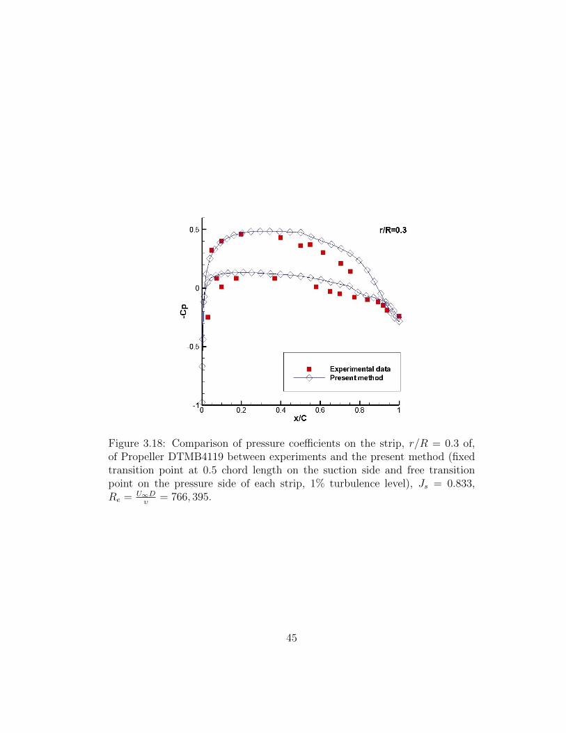
Figure 3.18: Comparison of pressure coefficients on the strip, r/R = 0.3 of,of Propeller DTMB4119 between experiments and the present method (fixedtransition point at 0.5 chord length on the suction side and free transitionpoint on the pressure side of each strip, 1% turbulence level), Js = 0.833,Re = U∞D
υ= 766, 395.
45

Figure 3.19: Comparison of pressure coefficients on the strip, r/R = 0.7 of,of Propeller DTMB4119 between experiments and the present method (fixedtransition point at 0.5 chord length on the suction side and free transitionpoint on the pressure side of each strip, 1% turbulence level), Js = 0.833,Re = U∞D
υ= 766, 395.
46

Figure 3.20: Comparison of pressure coefficients on the strip, r/R = 0.9 of,of Propeller DTMB4119 between experiments and the present method (fixedtransition point at 0.5 chord length on the suction side and free transitionpoint on the pressure side of each strip, 1% turbulence level), Js = 0.833,Re = U∞D
υ= 766, 395.
47

parts: one part is due to the friction on propeller blades and the other part is
due to the pressure. Panel methods ignore the effects of fluid viscosity, thus
cannot take the friction into consideration and cannot predict the influences
of boundary layer on pressure. An easy solution of this dilemma is to apply
empirical methods to consider the effects of fluid viscosity. However, such
method requires user adjustable corrections that are not general for all cases.
It has been proved that the viscous/inviscid interactive method can precisely
predict the changes of pressure on the wall due to boundary layer. For the
friction part, instead of using the empirical constants, the 3D viscous/inviscid
interactive method can predict more reasonable skin friction coefficient Cf
on propeller blades. Then the forces due to the friction are calculated by
integrating the shear stress τw = Cf · 12ρU2∞ over the blade surfaces. Fig. 3.21
shows the comparisons of KT and KQ between the experimental measurements
and the present method. The results predicted by the present method exhibit
considerable agreement with the experimental data.
3.4 Propeller NSRDC4381
The 3D viscous/inviscid interactive method is also applied to Propeller
NSRDC4381, which is a five-bladed propeller (shown in Fig. 3.22). The design
advance ratio Js of this propeller is 0.889. The results predicted by the present
method and RANS (ANSYS/FLUENT) simulations conducted by Tian and
Kinnas (2011) are compared. Fig. 3.23 shows the domain and boundary con-
ditions for RANS (ANSYS/FLUENT) simulations. The grid details are shown
48

Figure 3.21: Comparisons of KT and KQ of Propeller DTMB4119 at differentadvance ratios, between experiments and the present method.
49

in Fig. 3.24. Some important information of the RANS (ANSYS/FLUENT)
cases is listed in Table. 3.1.
Figure 3.22: Paneled geometry of Propeller NSRDC4381.
For the present 3D viscous/inviscid interactive method, it is necessary
to conduct a grid dependency study at first. The pressure distributions with
different numbers of panels along two strips on the propeller blade are com-
pared in Fig. 3.25. The great consistency shown in Fig. 3.25 indicates that the
changes of the number of panels on both chord and span wise directions do not
affect the final results. The pressure distributions at different iterations are
checked as well (shown in Fig. 3.26) to ensure the convergence of the results.
The 3D viscous/inviscid interactive method is applied to predict the
pressure on the blades of propeller 4381. Fig. 3.27 to Fig. 3.30 shows detailed
50

comparisons of pressure at two different operating conditions: the design con-
dition (Js = 0.889) and an off-design condition (Js = 0.5). The pressures
predicted by the present method show better correlation with the RANS re-
sults than those predicted by the panel method only, especially at the region
close to the blade trailing edge. Closer to the trailing edge, the effects of flu-
id viscosity become more significant and the boundary layer becomes thicker.
Thus more clear improvements of the results are observed in this region with
the boundary layer correction.
The thrust/torque forces due to the fluid viscosity is calculated by in-
tegrating the shear stress τ over the blade surfaces. Fig. 3.31 shows the
comparison of Cf predicted by the present method and RANS at the design
Figure 3.23: Domain and boundary conditions of the RANS (AN-SYS/FLUENT) case for Propeller NSRDC4381 (from Sharma 2011).
51

Figure 3.24: Grid details used in the RANS (ANSYS/FLUENT) case for Pro-peller NSRDC4381. Top left: O type grid on the propeller blade. Top right:grid details on the hub around the root section of the propeller blade. Bot-tom left: Grid details on the hub near the leading edge of the root section ofpropeller blade. Bottom right: grid details on the hub near the trailing edgeof the root section of the propeller blade. (from Sharma 2011).
52

(a) r/R=0.6 (b) r/R=0.9
Figure 3.25: Pressure distributions predicted by the present method usingdifferent numbers of panels at strips, r/R = 0.6 and r/R = 0.9, of PropellerNSRDC4381, Js = 0.889, Re = U∞D
υ= 7.42e5, 1% turbulence level, fixed
transition points at 0.1 chord length on both the pressure and suction sides ofeach strip.
53

Table 3.1: Information of the RANS (ANSYS/FLUENT) case for PropellerNSRDC4381
Cell number 1, 476, 540Reynolds number (J=0.889) 6.22e5Reynolds number (J=0.5) 4.15e5
Turbulence model k-ω SSTPressure correction scheme SIMPLEC
Spatial discretization QUICKTotal time for calculate (32 CPUs) 4,386 seconds
condition Js = 0.889. The comparison exhibits an acceptable agreement, in-
dicating that the present method could predict the friction on the propeller
blades. The plots of KT and KQ of this propeller at different operating condi-
tions are shown in Fig. 3.32. Compared with the experimental measurements,
(a) r/R=0.6 (b) r/R=0.9
Figure 3.26: Pressure distributions at different iterations at strips r/R = 0.6and r/R = 0.9 of Propeller NSRDC4381, predicted by the present method,Js = 0.889, Re = U∞D
υ= 7.42e5, 1% turbulence level, fixed transition points
at 0.1 chord length on both the pressure and suction sides of each strip.
54

(a) Full view (b) Detailed view close to trailing edge
Figure 3.27: Comparison of pressure distributions along the strip, r/R =0.6, of Propeller NSRDC4381, predicted by RANS (ANSYS/FLUENT), panelmethod and the present method (fixed transition points at 0.1 chord lengthon both the pressure and suction sides of each strip, 1% turbulence level),Js = 0.889, Re = U∞D
υ= 7.42e5 for viscous cases.
55

(a) Full view (b) Detailed view close to trailing edge
Figure 3.28: Comparison of pressure distributions along the strip, r/R =0.8, of Propeller NSRDC4381, predicted by RANS (ANSYS/FLUENT), panelmethod and the present method (fixed transition points at 0.1 chord lengthon both the pressure and suction sides of each strip, 1% turbulence level),Js = 0.889, Re = U∞D
υ= 7.42e5 for viscous cases.
56

(a) Full view (b) Detailed view close to trailing edge
Figure 3.29: Comparison of pressure distributions along the strip, r/R =0.6, of Propeller NSRDC4381, predicted by RANS (ANSYS/FLUENT), panelmethod and the present method (fixed transition points at 0.1 chord lengthon both the pressure and suction sides of each strip, 1% turbulence level),Js = 0.5, Re = U∞D
υ= 4.15e5 for viscous cases.
57

(a) Full view (b) Detailed view close to trailing edge
Figure 3.30: Comparison of pressure distributions along the strip, r/R =0.8, of Propeller NSRDC4381, predicted by RANS (ANSYS/FLUENT), panelmethod and the present method (fixed transition points at 0.1 chord lengthon both the pressure and suction sides of each strip, 1% turbulence level),Js = 0.5, Re = U∞D
υ= 4.15e5 for viscous cases.
58

the results predicted by the present method behave well near the design con-
dition, but under-estimate the KT and KQ at low Js (blow Js = 0.5). In fact,
at low J conditions, the effects of the wake become more significant. Thus
more accurate wake alignment schemes are needed. The results shown in Fig.
3.32 are obtained by the present method combined with PSF2 wake alignmen-
t. Kinnas et al. (2012) developed a new full wake alignment scheme FWA.
The results predicted by the present method with the full wake alignment
scheme are shown in Fig. 3.33, from which obvious improvements at low J are
observed.
(a) r/R=0.6 (b) r/R=0.74
Figure 3.31: Comparison of Cf at strips, r/R = 0.6 and r/R = 0.6, of PropellerNSRDC4381, between RANS (ANSYS/FLUENT) and the present method(fixed transition points at 0.1 chord length on both the pressure and suctionsides of each strip, 1% turbulence level), Js = 0.889, Re = U∞D
υ= 7.42e5.
59

Figure 3.32: Comparisons of KT and KQ of Propeller NSRDC4381 at differ-ent advance ratios, between the present method combined with PSF2 wakealignment and experiments.
60
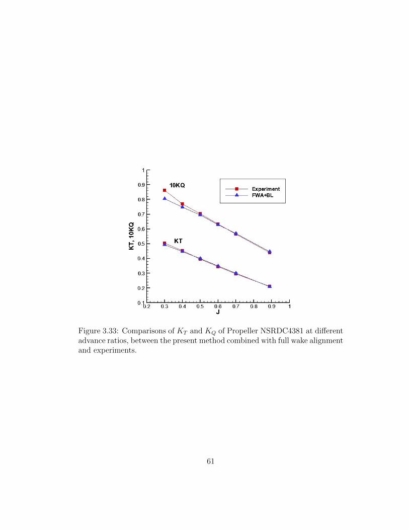
Figure 3.33: Comparisons of KT and KQ of Propeller NSRDC4381 at differentadvance ratios, between the present method combined with full wake alignmentand experiments.
61

3.5 DTMB Duct II
The 3D viscous/inviscid interactive method is applied to a bare duct
case. DTMB Duct II is an axis-symmetric duct, which has a NACA66 thick-
ness form, with a maximum thickness-chord ratio tmax/C = 0.1. The camber
has a NACA a = 0.8 mean distribution and the maximum camber-chord ra-
tio is fmax/C = 0.04. Fig. 3.34 shows the paneled geometry of this duct.
The duct is placed at zero angle of attack. The Reynolds number Re = U∞Dν
is 2.06 × 10⁶. The pressure on the duct predicted by the present method is
compared with the measurements by Morgan and Caster (1965).
Figure 3.34: Paneled geometry of the DTMB Duct II.
The result (pressure) of a grid dependency study is shown in Fig. 3.35.
Using different numbers of panels on the chord and span wise directions, the
62

plots of the pressures predicted by the current method collapse into the same
line. Fig. 3.36 shows the convergence process of the pressure. At the 5th
iteration, converged results are obtained. Since DTMB Duct II is an axis-
symmetric duct and the angle of attack is zero, it is expected that the pressure
or the boundary layer variables be the same at different sections along the
chord wise direction. The pressure and the displacement thickness of boundary
layer at three selected strips along chord wise direction are checked and shown
in Fig. 3.37 and Fig. 3.38, respectively.
x/c
-Cpvis
0 0.2 0.4 0.6 0.8
-0.8
-0.6
-0.4
-0.2
0
0.2
60 X 90
60 X 100
80 X 100
Figure 3.35: Pressure distributions on DTMB Duct II predicted by the presentmethod using different numbers of panels on both the chord and span wisedirections, Re = U∞D
υ= 2.06e6, fixed transition points at 0.05 chord length on
both the pressure and suction sides of each strip, 1% turbulence level.
Fig. 3.39 shows the predicted invsicid (panel method only) and viscous
63
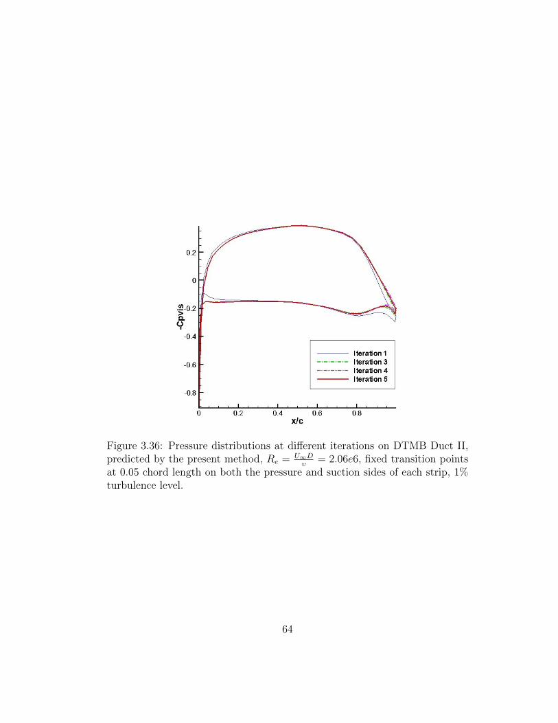
Figure 3.36: Pressure distributions at different iterations on DTMB Duct II,predicted by the present method, Re = U∞D
υ= 2.06e6, fixed transition points
at 0.05 chord length on both the pressure and suction sides of each strip, 1%turbulence level.
64

Figure 3.37: Pressure distributions along three different sections of DTMBDuct II, predicted by the present method, Re = U∞D
υ= 2.06e6, fixed transition
points at 0.05 chord length on both the pressure and suction sides of each strip,1% turbulence level.
65
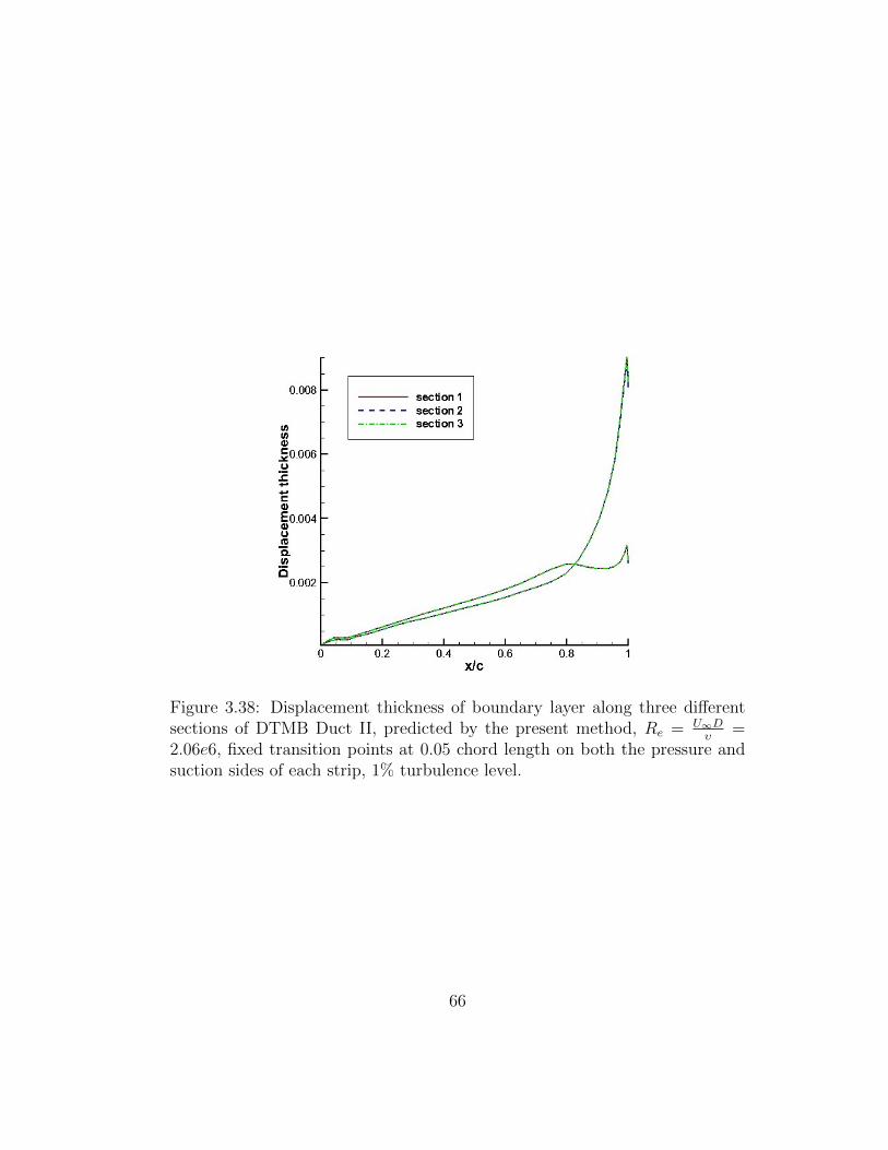
Figure 3.38: Displacement thickness of boundary layer along three differentsections of DTMB Duct II, predicted by the present method, Re = U∞D
υ=
2.06e6, fixed transition points at 0.05 chord length on both the pressure andsuction sides of each strip, 1% turbulence level.
66

(present method) pressure on the duct strip compared with the experimental
measurements from Morgan and Caster (1965). Both the viscous and inviscid
solution show good correlations with the experiment data.
Figure 3.39: Viscous and inviscid pressure distributions on the DTMB Duct IIpredicted by the present method (fixed transition points at 0.05 chord lengthon both the pressure and suction sides of each strip, 1% turbulence level),compared with the experimental measurements by Morgan and Caster (1965),Re = U∞D
υ= 2.06e6.
67

Chapter 4
Viscous Image Model
In this chapter, the image model used to simulate the effects of slip
walls developed by Singh (2009) is introduced. The author further improves
this model for viscous cases. A case of a straight wing blade between two
slip walls is carried out, and the results are compared with those of a RANS
case. Next, the results of a case of a swept wing blade between two slip ways
are presented and analyzed. The slip walls exclude the effects of the blade
tip, so that the 3D viscous/inviscid interactive is more easy to be applied.
In addtion, the case of the straight wing between two parallel slip walls is
expected equivalent with a 2D case, which is a good test to validate the 3D
viscous/inviscid interactive method.
4.1 Image Model with Panel Method Only
Singh (2009) introduced an image model to simulate the effects of slip
walls. For instance, the system of a wing blade adjacent to a slip wall shown
in Fig. 4.1 is equivalent to the one shown in Fig. 4.2. In Fig. 4.2, the effects
of the slip wall are considered by mirroring the wing blade about the wall, so
that the derivative of any variable cross the red line is zero as the effects of
68

the slip wall in Fig. 4.1.
Figure 4.1: Diagram of a straight wing blade adjacent to a slip wall
Figure 4.2: Diagram of a straight wing blade and its images, symmetric aboutthe red line
Since the wing blade and its image shown in Fig. 4.2 are symmetric
about the wall, the potential on a panel of the wing blade should be the same
69

with that on the corresponding image panel symmetric about the wall. With
this statement, the inviscid solution of this case can be obtained by solving
(2.12), but with new influence coefficients to consider the effects of the image.
The new influence coefficients are expressed as:
Anewij = Aij + Aij′ (4.1)
Snewij = Sij + Sij′ (4.2)
where j′ is the image panel corresponding to the original panel j on the wing
blade. One useful fact is that the source or dipole influence coefficient due to
an image panel at a particular control point is the same as the one due to the
original panel at the image control point (shown in Fig. 4.3). According to
this fact, the influence coefficients can be rewritten as:
Anewij = Aij + Ai′j (4.3)
Snewij = Sij + Si′j (4.4)
The new expressions are very useful for the simplification of coding. When
multiple images are considered, the influence coefficients become:
Anewij = Aij +
Image∑i′
Ai′j (4.5)
Snewij = Sij +
Image∑i′
Si′j (4.6)
where Image is the number of images. With the new influence coefficients,
the inviscid solution can be obtained by solving (2.12).
70

Figure 4.3: Diagram of the equivalence of the influence coefficients, from Singh(2009)
4.2 Image Model with 3D Viscous/Inviscid InteractiveMethod
Once the inviscid solution is obtained, blowing sources with unknown
strengths are added on the panels of the original wing blade, the wake and
their images to consider the effects of fluid viscosity. Analogous to (3.1), the
viscous velocity becomes:
U ei,m =
∂Φi,m
∂s
= U invi,m +
N+NW∑j=1
Di,j,mmj,m +mr∑
k=1,k 6=m
N+NW∑j=1
Di,j,kmj,k
+
Imag∑im=1
mr∑k=1
N+NW∑j=1
Di,j,k,immj,k,im
(4.7)
71

where Image is the number of images. Using the same iterative scheme de-
scribed in Fig. 3.11, The unknown mass defects in (4.7) can be resolved. In
this case, the last two terms on the right hand side of (4.7) should be updated
each iteration and added to the inviscid velocity term.
4.3 Straight Wing between Two Parallel Slip Walls
A case of a 3D straight wing blade between two parallel walls (shown in
Fig. 4.4) subject to a uniform inflow with a 2 degree angle of attack is carried
out. For this case, infinite images are required on both sides to simulate the
effects of the two parallel walls. Practically, a reasonable number of images
can be determined through convergence studies to obtained fairly accurate
numerical results.
Figure 4.4: Diagram of a wing blade between two parallel walls
The result (pressure) of a grid dependence study is presented in Fig.
4.5. The plots of the pressure coefficients along the strip at r/R = 0.75
obtained using different numbers of panels on both span wise and chord wise
72

directions collapse into the same line. In other words, the changes of the
number of panels do not affect the final result, indicating a good convergence
character of the present method and the code.
Figure 4.5: Pressure distributions along the strip at r/R = 0.75, predicted bythe present method using different numbers of panels on span and chord wisedirections, Re = U∞c
υ= 1.0e6, fixed transition points at 0.1 chord length on
both the pressure and suction sides of each strip, 1% turbulence level.
A convergence study is conducted to determine a reasonable number of
images to simulate the effects of the two parallel slip walls. Different numbers
of images on each side are selected, and the predicted circulations are plotted
in Fig. 4.6, from which the circulation is converging with the increase of the
image number. The viscous and invscid pressure distributions along the strip
73
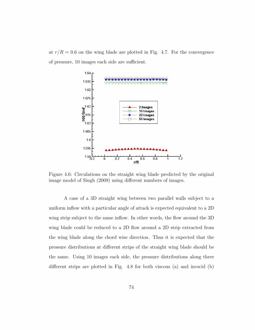
at r/R = 0.6 on the wing blade are plotted in Fig. 4.7. For the convergence
of pressure, 10 images each side are sufficient.
Figure 4.6: Circulations on the straight wing blade predicted by the originalimage model of Singh (2009) using different numbers of images.
A case of a 3D straight wing between two parallel walls subject to a
uniform inflow with a particular angle of attack is expected equivalent to a 2D
wing strip subject to the same inflow. In other words, the flow around the 3D
wing blade could be reduced to a 2D flow around a 2D strip extracted from
the wing blade along the chord wise direction. Thus it is expected that the
pressure distributions at different strips of the straight wing blade should be
the same. Using 10 images each side, the pressure distributions along three
different strips are plotted in Fig. 4.8 for both viscous (a) and invscid (b)
74

(a) Viscous (b) Inviscid
Figure 4.7: Pressure distributions along the strip at r/R = 0.6 of the straightwing blase, predicted by the original and the present image model, using d-ifferent numbers of images. For the viscous case, Re = U∞c
υ= 1.0e6, fixed
transition points at 0.1 chord length on both the pressure and suction sides ofeach strip, 1% turbulence level.
75

cases. The plots of the pressure distributions collapse into the same line, as
expected.
(a) Viscous (b) Inviscid
Figure 4.8: Pressure distributions on the strips at r/R = 0.3, r/R = 0.5and r/R = 0.9 of the straight wing blade, predicted by the original and thepresent image model, using different numbers of images. For the viscous case,Re = U∞c
υ= 1.0e6, fixed transition points at 0.1 chord length on both the
pressure and suction sides of each strip, 1% turbulence level.
A 2D and a 3D RANS case are carried out as references. The domain for
the 3D RANS case is shown in Fig. 4.9. H type grid topology is used around
the wing blade as shown in Fig. 4.10. The symmetry boundary condition
is applied to the side boundaries ABC and DEF to simulate the parallel slip
walls. The outlet ABFD is set as the outflow. The rest boundaries are set
as the velocity inflow with the a specified velocity. The value of y+ on the
wing surface is ranged between 30 and 50. Some related information about
the 3D RANS case is listed in Table 4.1. A section along the chord wise
76
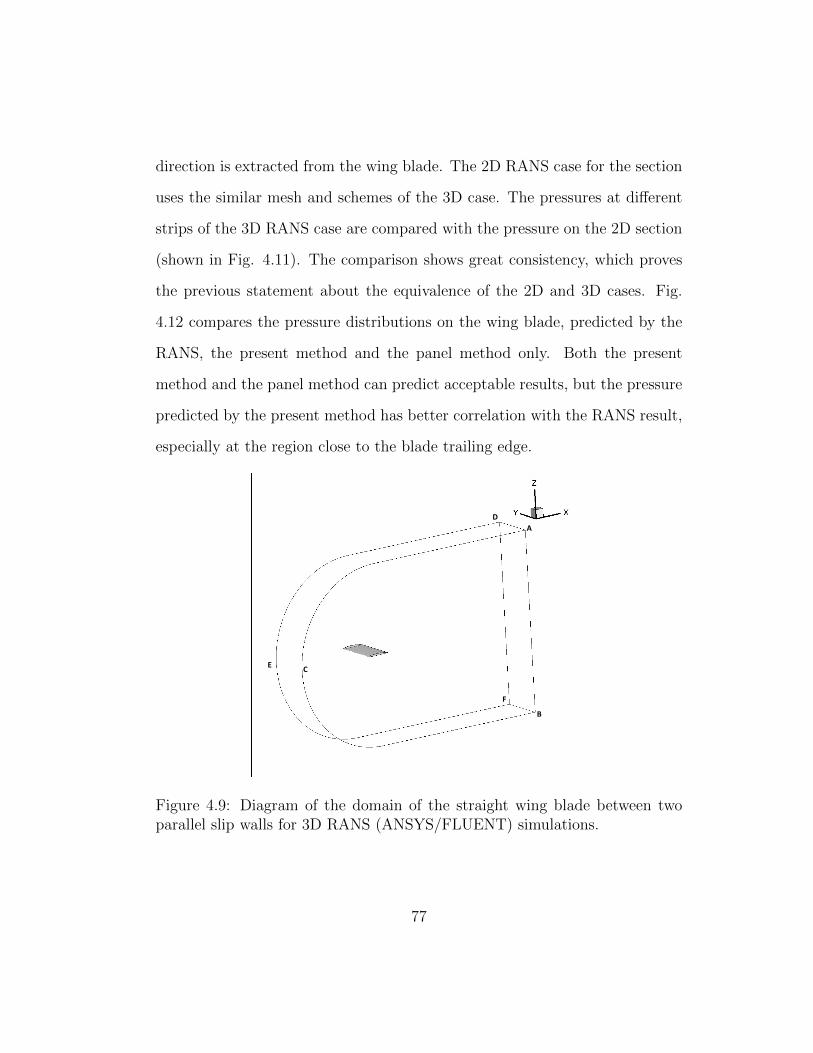
direction is extracted from the wing blade. The 2D RANS case for the section
uses the similar mesh and schemes of the 3D case. The pressures at different
strips of the 3D RANS case are compared with the pressure on the 2D section
(shown in Fig. 4.11). The comparison shows great consistency, which proves
the previous statement about the equivalence of the 2D and 3D cases. Fig.
4.12 compares the pressure distributions on the wing blade, predicted by the
RANS, the present method and the panel method only. Both the present
method and the panel method can predict acceptable results, but the pressure
predicted by the present method has better correlation with the RANS result,
especially at the region close to the blade trailing edge.
A
B
C
D
E
F
Figure 4.9: Diagram of the domain of the straight wing blade between twoparallel slip walls for 3D RANS (ANSYS/FLUENT) simulations.
77

Y X
Z
Figure 4.10: Grid details around the straight wing blade used in 3D RANS(ANSYS/FLUENT) simulations.
78

Figure 4.11: Pressure coefficients on the strips at r/R=0.2 and r/R=0.6 ofthe 3D straight wing predicted by the 3D RANS (ANSYS/FLUENT) case,and on the 2D strip predicted by the 2D RANS (ANSYS/FLUENT) case,Re = U∞c
υ= 1.0e6.
79
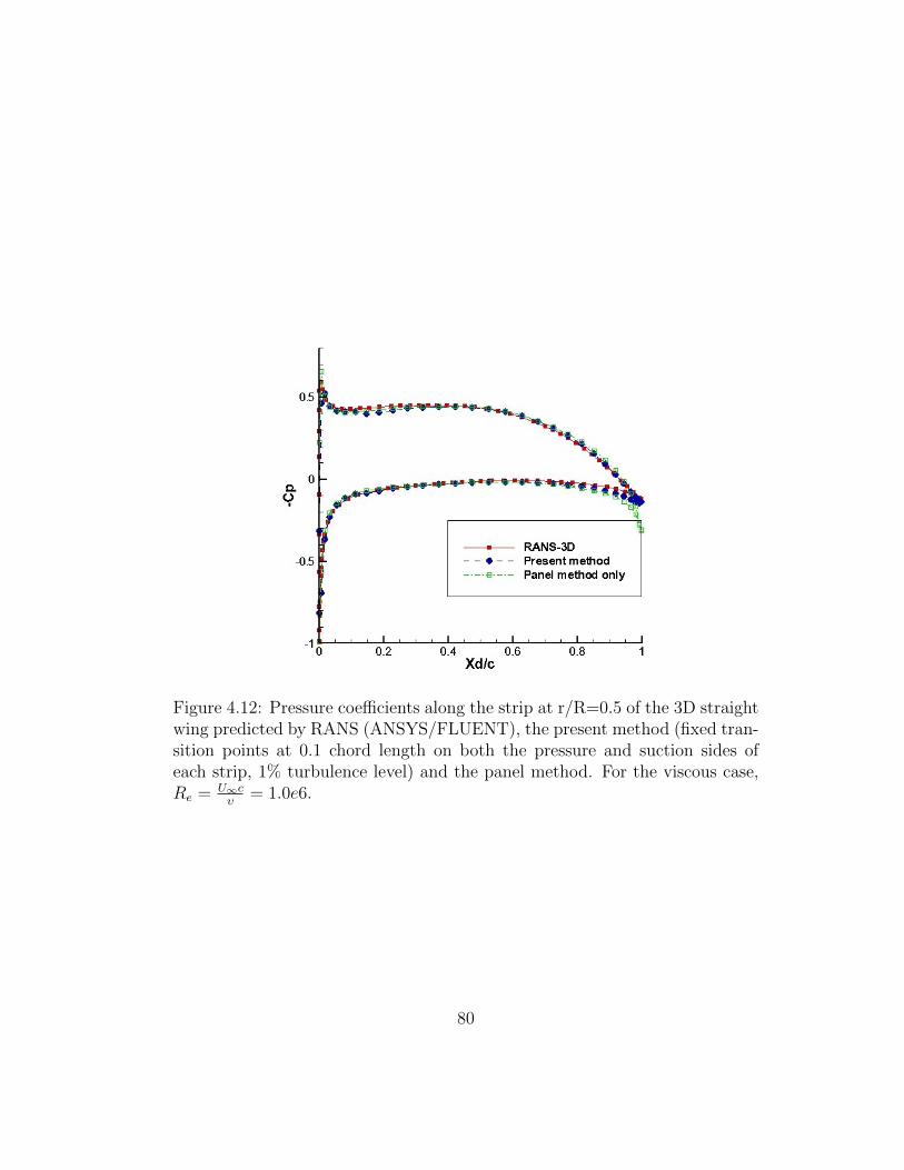
Figure 4.12: Pressure coefficients along the strip at r/R=0.5 of the 3D straightwing predicted by RANS (ANSYS/FLUENT), the present method (fixed tran-sition points at 0.1 chord length on both the pressure and suction sides ofeach strip, 1% turbulence level) and the panel method. For the viscous case,Re = U∞c
υ= 1.0e6.
80

Table 4.1: Information of the RANS (ANSYS/FLUENT) case for a straightwing blade between two parallel slip walls.
Cell number 537, 080Reynolds number 1e6Turbulence model k-ω SST
Pressure correction scheme SIMPLECSpatial discretization Second order upwind
Total time for calculate (32 CPUs) 20 mins
4.4 Swept Wing between Two Parallel Slip Walls
A case of a 3D swept wing blade between two parallel walls shown
in Fig. 4.13 subject to a uniform flow with a 2 degree angle of attack is
carried out. The pressures along different strips are plotted in Fig. 4.14. The
differences among the plots imply that the case is not equivalent to a simple 2D
strip case. The pressures predicted by the present method are also correlated
with RANS results in Fig. 4.15, Fig. 4.16 and Fig. 4.17. The comparisons
show great agreements.
81

Figure 4.13: Diagram of a swept wing between two parallel slip walls.
Xd/C
-Cp
0.2 0.4 0.6 0.8
-0.6
-0.4
-0.2
0
0.2
0.4
0.6
0.8
1r/R=0.3
r/R=0.6
r/R=0.9
(a) Viscous
Xd/C
-Cp
0.2 0.4 0.6 0.8
-0.6
-0.4
-0.2
0
0.2
0.4
0.6
0.8
1 r/R=0.3
r/R=0.6
r/R=0.9
(b) Inviscid
Figure 4.14: Pressure distributions on the strips at r/R = 0.3, r/R = 0.5 andr/R = 0.9 of the wing blade, predicted by the present method, Re = U∞c
υ=
1.0e6, fixed transition points at 0.1 chord length on both the pressure andsuction sides of each strip, 1% turbulence level.
82

x/c
-Cp
0 0.2 0.4 0.6 0.8 1-0.8
-0.6
-0.4
-0.2
0
0.2
RANS
Viscous Image Model
Inviscid Image Model
r/R=0.025
Figure 4.15: Pressure coefficients on the strip at r/R=0.025 of the 3D swep-t wing, predicted by the 3D RANS (ANSYS/FLUENT) case, the presentmethod (fixed transition points at 0.1 chord length on both the pressure andsuction sides of each strip, 1% turbulence level) and the panel method. Forthe viscous case, Re = U∞c
υ= 1.0e6.
83

x/c
-Cp
0 0.2 0.4 0.6 0.8 1
-0.5
0
0.5
RANS
Viscous Image model
Inviscid Image Model
r/R=0.5
Figure 4.16: Pressure coefficients on the strip at r/R=0.5 of the 3D swep-t wing, predicted by the 3D RANS (ANSYS/FLUENT) case, the presentmethod (fixed transition points at 0.1 chord length on both the pressure andsuction sides of each strip, 1% turbulence level) and the panel method. Forthe viscous case, Re = U∞c
υ= 1.0e6.
84

x/c
-Cp
0 0.2 0.4 0.6 0.8 1
-0.5
0
0.5
1
1.5
2
RANS
Viscous Image Model
Inviscid Image Model
r/R=0.975
Figure 4.17: Pressure coefficients on the strip at r/R=0.975 of the 3D swep-t wing, predicted by the 3D RANS (ANSYS/FLUENT) case, the presentmethod (fixed transition points at 0.1 chord length on both the pressure andsuction sides of each strip, 1% turbulence level) and the panel method. Forthe viscous case, Re = U∞c
υ= 1.0e6.
85

Chapter 5
Hydrofoils and Propellers with Non-Zero
Trailing Edge Thickness
In this chapter, the extension scheme for 2D hydrofoils with non-zero
thickness trailing edges or open trailing edges proposed by Pan (2009, 2011)
is further improved. First, a new extension and search scheme in 2D are
introduced in details. Then results of two sample cases are presented and
correlated with those of RANS cases. A similar method for 3D blades with
non-zero trailing edge thickness is introduced next. The method is applied to
a 3D propeller as a sample case and some preliminary inviscid (panel method
only) results are presented.
5.1 2D Hydrofoils with Non-Zero Trailing Edge Thick-ness
5.1.1 Open Trailing Edge Extension Scheme
Panel methods have difficulties dealing with hydrofoils or propeller
blades with non-zero thickness trailing edges. In one instance, Fig. 5.1 shows
the trailing edge of a strip extracted from the ONR-AxWj-2 rotor blade. Gen-
erally, such a trailing edge with finite thickness needs to be closed (shown in
Fig. 5.2) for panel methods. However, for the trailing edge with large thick-
86

ness, this method may change the original geometry too much. Pan (2009,
2011) proposed a scheme that extends the trailing edge with non-zero thick-
ness to form a sharp one (shown in Fig. 5.3).
Finite thickness
Figure 5.1: Section with a non-zero thickness trailing edge, extracted from theONR-AxWj-2 rotor blade
Given the last camber point, the method by Pan (2009, 2011) gener-
ates a new camber and thickness distributions by interpolation of the original
foil and the last camber point. One flaw of this scheme is that the original
geometry may be changed once an inappropriate last camber point is given.
A new extension scheme that uses second order polynomials to describe the
extension edges (as shown in Fig. 5.4) is introduced to overcome the problem
of Pan (2009, 2011). Define the two end points of the upper and lower side
of the open trailing edge as the cut points as shown in Fig. 5.4. The new
scheme estimates the last camber point based on the slopes of the two cut
points, so that inappropriate input point can be avoided. Then two second
87
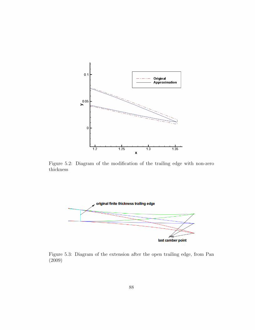
Figure 5.2: Diagram of the modification of the trailing edge with non-zerothickness
Figure 5.3: Diagram of the extension after the open trailing edge, from Pan(2009)
88

order polynomials are determined to describe the upper and lower edges of the
extension. Suppose the lower side BC of the extension (shown in Fig. 5.4)
can be described as:
y = ax2 + bx+ c (5.1)
where a, b and c are constant unknowns. The three constants should satisfy
the following conditions:
yB = ax2B + bxB + c
yC = ax2C + bxC + c(dy
dx
)B
= 2axB + b
(5.2)
where the third equation ensures the continuity at point B. The expression of
the lower side BC of the extension can be determined by solving (5.2). The
upper side can be determined similarly.
5.1.2 Search Scheme for Extension
Since the extension after the open trailing edge is an artificial part, it
should satisfy the two following conditions:
• No-lift condition
The lift of the extension part should be zero.
• Pressure equivalence condition
The pressures of the cut points should be same.
In fact, the second condition is the primary one to be satisfied. The first con-
dition is always satisfied with the second one. To satisfy the second condition,
89

the estimated last camber point is moved vertically to search the correct po-
sition. Assume that the pressure difference ∆p between the two cut points is
a function of the vertical position of the last camber point yC .
∆p = f(yC)
d(∆p) =df(yC)
dyCdyC
(5.3)
where the derivative df(yC)dyC
can be calculated numerically. The search scheme
is shown in Fig. 5.5. First, the last camber point based on the slopes of the
cut points is estimated. Then extend the trailing edge with the new scheme
to form a sharp one and calculate the pressure difference ∆p between the cut
points. Next, update the vertical position of the last camber point yC by (5.3)
and extend the trailing edge again. Repeat this process until ∆p becomes zero.
Cut points
C
B
Figure 5.4: Diagram of extension of the trailing edge with non-zero thickness
90

Estimate the last camber point
Calculate Δ𝑝 of the cut
points
Update the vertical position
of the last camber point 𝑦𝐶
Initially 𝑈𝑒 = 𝑈𝑖𝑛𝑣
CalculateΔ𝑝 of the cut points
Δ𝑝=0?
No
Yes Final results
Figure 5.5: Diagram of the procedure of the search scheme for extension
5.2 Sample Cases of 2D Hydrofoils
5.2.1 Strip of ONR-AxWj-2 Rotor Blade
The method described above is applied to a 2D strip extracted from
the ONR-AxWj-2 rotor blade at r/R = 0.7. The pressure predicted by the
91

present method has a great correlation with RANS results, shown in Fig. 5.6.
The final pressure difference of the two cut points ∆p is 1.95e − 3, and the
lift on the extension part is less than 0.3 percent of the total lift on the strip,
which satisfies both the zero lift and the pressure equivalence conditions. The
final extension of the trailing edge is shown in Fig. 5.7. The recorded pressure
difference ∆p of the two cut points and the vertical position of the last camber
point yC shows a linear relationship in Fig. 5.8.
Figure 5.6: Comparison of pressure distributions on the strip extractedfrom the ONR-AxWJ-2 rotor blade at r/R = 0.7, between RANS (AN-SYS/FLUENT) and the present method (fixed transition points at 0.01chord length on both the pressure and suction sides, 1% turbulence level),Re = U∞c
υ= 5.0e6.
92

Figure 5.7: Final extension behind the the strip extracted from the ONR-AxWJ-2 rotor blade at r/R = 0.7, predicted by the present method, Re =U∞cυ
= 5.0e6, fixed transition points at 0.01 chord length on both the pressureand suction sides, 1% turbulence level.
93

Figure 5.8: Pressure difference ∆p of the cut points vs. vertical position ofthe last camber point yC , of the ONR-AxWJ-2 rotor blade at r/R = 0.7, fromthe present method, Re = U∞c
υ= 5.0e6, fixed transition points at 0.01 chord
length on both the pressure and suction sides, 1% turbulence level.
94

5.2.2 NACA Hydrofoil
Another sample case is a 2D NACA hydrofoil ( fmax/c = 0.02 , tmax/c =
0.04) with a vertical cut at the 90 percent chord length treated as a trailing edge
with non-zero thickness. The pressure difference ∆p of the final result is 3.19e−
4. The lift of the extension part is around 0.5 percent of the total lift. Fig. 5.9
compares the pressure along the section predicted by the present method and
RANS. The great agreement of the comparison validates the present method.
The final extension behind the open trailing edge is shown in Fig. 5.10, and
the linear relationship between ∆p and yC is shown in Fig. 5.11.
Figure 5.9: Comparison of pressure distributions along the NACA hydrofoilwith a non-zero thickness trailing edge, between RANS (ANSYS/FLUENT)and the present method (fixed transition points at 0.01 chord length on boththe pressure and suction sides, 1% turbulence level), Re = U∞c
υ= 9.0e6.
95

Figure 5.10: Final extension behind the NACA hydrofoil with a non-zerothickness trailing edge, predicted by the present method, Re = U∞c
υ= 5.0e6,
fixed transition points at 0.01 chord length on both the pressure and suctionsides, 1% turbulence level.
96

Figure 5.11: Pressure difference ∆p of the cut points vs. vertical position of thelast camber point yC , of the NACA hydrofoil with a non-zero thickness trailingedge, from the present method, Re = U∞c
υ= 5.0e6, fixed transition points at
0.01 chord length on both the pressure and suction sides, 1% turbulence level.
97

5.3 Propeller Blades with Non-zero Trailing Edge Thick-ness
For 3D propeller blades with non-zero thickness trailing edges, each
blade is divided into several strips along the constant radius. The trailing
edge of each strip is extended using the extension scheme used in 2D hydrofoil
cases. Next, the Newton’s method is used to search the correct positions of
the last camber points of the extensions so that the no-lift and the pressure
equivalence (primary one) conditions are satisfied. In 3D cases, the pressure
difference ∆p between the cut points of one section is a function of the vertical
positions of the last camber points of all the sections (yc,1, yc,2 . . . yc,mr).
∆p1 = f1 (yc,1, yc,2 . . . yc,mr)
∆p2 = f2 (yc,1, yc,2 . . . yc,mr)
. . .
∆pmr = fmr (yc,1, yc,2 . . . yc,mr)
(5.4)
where mr is the number of strips on a blade. (5.4) leads to the following
relationship:
d
∆p1∆p1. . .
∆pmr
=
∂f1∂yc,1
∂f1∂yc,2
. . . ∂f1∂yc,mr
∂f2∂yc,1
∂f2∂yc,2
. . . ∂f2∂yc,mr
. . . . . . . . . . . .∂fmr∂yc,1
∂fmr∂yc,2
. . . ∂fmr∂yc,mr
d
yc,1yc,2. . .yc,mr
(5.5)
The Jacobin matrix in (5.5) could be calculated numerically. The last camber
points of the strips are moved vertically a small amount one by one. Each time,
the pressure difference between the cut points of each strip is evaluated. The
derivatives in the matrix are calculated by dividing the corresponding pressure
98

differences by the small movement. Once the initial positions of the last camber
points of the strips are estimated, the pressure difference ∆p between the cut
points of each strip could be evaluated. Then the positions of the last camber
points of all the strips are updated following (5.5). Repeat the process until
the pressure equivalence condition is satisfied on all the strips.
A five-bladed propeller with non-zero thickness trailing edge (studied
in Pan 2009) is used in this study. The details of the propeller geometry are
restricted to show in this thesis. A global view of this propeller is shown in
Fig. 5.12. The extension scheme described in the 2D case is applied to each
strip of the propeller blade. The initial modified geometry is shown in Fig.
5.13.
Figure 5.12: Propeller with non-zero trailing edge thickness, from Pan (2009).
99
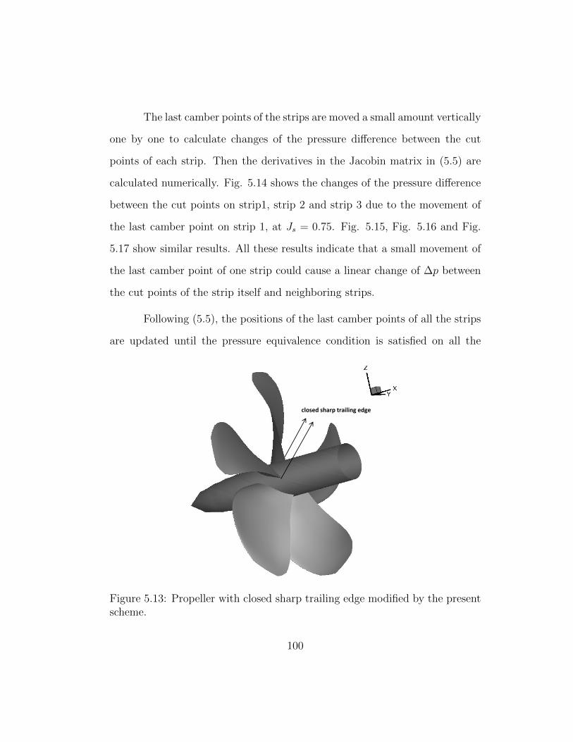
The last camber points of the strips are moved a small amount vertically
one by one to calculate changes of the pressure difference between the cut
points of each strip. Then the derivatives in the Jacobin matrix in (5.5) are
calculated numerically. Fig. 5.14 shows the changes of the pressure difference
between the cut points on strip1, strip 2 and strip 3 due to the movement of
the last camber point on strip 1, at Js = 0.75. Fig. 5.15, Fig. 5.16 and Fig.
5.17 show similar results. All these results indicate that a small movement of
the last camber point of one strip could cause a linear change of ∆p between
the cut points of the strip itself and neighboring strips.
Following (5.5), the positions of the last camber points of all the strips
are updated until the pressure equivalence condition is satisfied on all the
closed sharp trailing edge
Figure 5.13: Propeller with closed sharp trailing edge modified by the presentscheme.
100

Figure 5.14: Pressure differences between the cut points of strip 1 and neigh-boring strips vs. the movement of the last camber point of strip 1.
Figure 5.15: Pressure differences between the cut points of strip 5 and neigh-boring strips vs. the movement of the last camber point of strip 5.
101
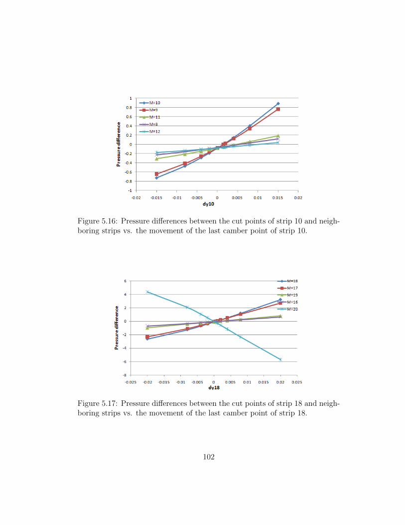
Figure 5.16: Pressure differences between the cut points of strip 10 and neigh-boring strips vs. the movement of the last camber point of strip 10.
Figure 5.17: Pressure differences between the cut points of strip 18 and neigh-boring strips vs. the movement of the last camber point of strip 18.
102

strips. The pressure difference between the cut points of each strips is plotted
in Fig. 5.18. The blue line represents ∆p on the initial extension. The red
line represents the results on the final extension (after several updates of the
last camber points). The pressure equivalence condition is satisfied on most
strips after four iterations. For the strips very close to the hub and the tip,
however, the pressure differences between the cut points do not decrease very
obviously, this is because the movements of the last camber points on these
strips are restrained to avoid abrupt changed along the trailing edge curve. The
circulation on the final blade geometry is plotted in Fig. 5.19. The smooth
curve of the circulation indicates the final blade geometry is acceptable and
ready for further studies. However, it should be noticed that the success of the
3D search scheme in this case will not necessarily guarantee the success in other
cases. Because the derivatives in the Jacobin matrix calculated numerically
are only accurate when the movements of the last camber points are restrained
in a small amount around the initial positions. In other cases (different Js),
the 3D search scheme may lead some large movements of the last camber
points. The changes of the pressure differences due to the large movements
will be different from the indication of the derivatives in the Jacobin matrix.
Therefore, the movement of the last camber point on each strip should be
restrained around the initial position, when large movements are calculated
by the 3D search scheme. Another reason of restraining the movements of the
last camber points is to avoid abrupt changes of the extended trailing edge
and ensure that the trailing edge follows a smooth curve.
103

Figure 5.18: Pressure differences between the cut points on the initial and finalextensions.
r/R
100Gr
0.2 0.4 0.6 0.8 1
0
0.2
0.4
0.6
0.8
Figure 5.19: Circulation on the final blade geometry.
104

The thrust/torque forces predicted by the present method, Pan (2009)
and experiment are plotted in Fig. 5.20 and Fig. 5.21. The results of the
present method show a better correlation with experimental measurements
than those in Pan (2009). In fact, the results of Pan (2009) had been improved
in Pan and Kinnas (2011) by using a full wake alignment. At this stage,
the combination of the improved method and the full wake alignment is not
available. Thus the same wake alignment in Pan (2009) is still used to study
the effects of the present method. The results by the present method are
expected to be improved when further coupled with the full wake alignment
used in Pan and Kinnas (2011).
Js
KT
0.7 0.75 0.8 0.85 0.9 0.95 1-0.04
-0.02
0
0.02
0.04
0.06
0.08
0.1
0.12
0.14
Experiment
Pan (2009)
Present method
Figure 5.20: KT of the propeller with finite thickness trailing edge.
105

Js
10KQ
0.7 0.75 0.8 0.85 0.9 0.95 10
0.05
0.1
0.15
0.2
0.25
Experiment
Pan (2009)
Present method
Figure 5.21: KQ of the propeller with finite thickness trailing edge.
106

Chapter 6
Conclusions and Recommendations
6.1 Conclusions
In this thesis, a 3D viscous/inviscid interactive method has been de-
veloped, by coupling a 3D low-order potential based panel method and a 2D
integral boundary layer analysis method, for predicting the effects of fluid vis-
cosity on the performance of fully wetted propellers. The author follows the
assumption that the effects of the boundary layer along the span direction (ra-
dially outward of propeller blades) are small compared with those along the
stream wise direction (along constant radius of propeller blades). The assump-
tion allows one to simplify the 3D boundary layer into 2D on the strips along
the stream wise direction and to avoid solving the 3D integral boundary layer
equations. This method has been successfully applied to propeller, duct, and
hydrofoil cases and shows great correlations with experimental measurements
or RANS results. One significant improvement of this method, as compared
with previous work, is to further consider the viscous effects of neighboring
strips and blades.
Contributions of the present work include:
• The 3D viscous/inviscid interactive method considers the 3D boundary
107

layer on propeller blades or hydrofoils comprehensively, but with less
computation expense by applying a reasonable assumption. Previously,
a complete 3D viscous/inviscid interactive method by Milewski (1997)
was developed by coupling a panel method with the 3D integral bound-
ary layer equations. Such method requires large amounts of computer
resources and is difficult to be applied to complicated geometries such
propeller blades. Hufford (1992, 1994) and Sun (2008) assumed that the
3D boundary layer on propeller blades could be reduced into 2D on strips
along the constant radius. The author in this thesis follows their assump-
tion but further considers the viscous effects from neighboring strips and
blades by a 3D wall transpiration model. The effects of the neighboring
blades turns out to be very limited, but the effects of other strips lead
to obvious corrections of the pressure distributions on propeller blades.
• The present method can predict the friction on propeller blades more
accurately than empirical methods. Generally, such empirical methods
use empirical constants as the friction coefficients to take the effects of
fluid viscosity into account. The present method provides a better way
of predicting the skin friction coefficient. Through some cases in the
thesis, it is proven that the predicted friction coefficients by the present
method are much more reasonable than any empirical constant.
• The 3D viscous/inviscid interactive method is also applied to develop a
viscous image model. Singh (2009) developed an image model to simulate
108

the effects of slip walls. This model was developed based on a pertur-
bation potential based panel method and was limited only for inviscid
cases. A new viscous image model is developed in this thesis by cou-
pling the original model of Singh and the 3D viscous/inviscid interactive
method. The new model is applied to cases of wing blades between two
parallel slip walls, and the results show better correlation with RANS.
• The method proposed by Pan (2009,2011) for hydrofoils or propeller
blases with non-zero thickness trailing edges is improved. Panel methods
have some difficulties dealing with such trailing edges. This scheme
extends the trailing edge with finite thickness to form a sharp one for
panel methods. The geometry of the extension keeps changing until
two conditions, the no-lift and the pressure equivalence condition, on
the extension part are satisfied. The author in this thesis follows the
basic ideal of the method of Pan, but proposes a new extension and an
improved search scheme to make this method more reliable.
6.2 Recommendations
The present method produces accurate predictions of the effects of fluid
viscosity on propeller flows, but further improvements could be achieved in
future research.
• To improve the efficiency of calculations, the present 3D viscous/inviscid
interactive method only considers the boundary layer along the stream
109

wise direction, but ignores the one of crossing flow. Even though this is a
reasonable assumption, the boundary layer of the crossing flow may still
have some influences on the final results in some cases. In one instance,
for the DTMB Duct II case, the results predicted by the present method
are changed if the panels on the duct are given a large pitch angle. This
is because the panels with the pitch angle make the divided strips away
from the steam wise direction. In other words, the boundary layer is not
considered in the correct direction. In such situations, the effects of the
boundary layer on the other direction cannot be negligible.
• The method proposed by Pan (2009, 2011) for 2D hydrofoils with non-
zero thickness trailing edges has been improved and successfully applied
to two sample cases in 2D in the thesis. However, the study of 3D
cases is very limited. The search scheme for 3D blades should consider
the interactions among the strips by Newton’s method. The derivatives
used in the scheme can only be calculated numerically. Even though
the numerical derivatives of the sample case studied in this thesis seems
fine, the accuracy still cannot be guaranteed. Pan (2009, 2011) had to
sacrifice the efficiency of calculations and deal with the strips one by
one. Therefore, more studies and research should be conducted in the
future to make the method for 3D cases more reasonable and reliable. In
addition, the present method should be further coupled with a full wake
alignment to improve the predicted KT and KQ.
110

Appendix
111

Appendix 1
Evaluation of Influence Coefficients
In this appendix, the formulations of the influence coefficients for 2D
and 3D panels are presented.
1.1 2D Influence Coefficients
• Dipole
dij =1
2π
∫∂ ln r
∂ndS (1.1)
• Source
sij =1
2π
∫ln rdS (1.2)
1.2 3D Influence Coefficients
• Dipole
dij = − 1
4π
∫∂(1/r)
∂ndS (1.3)
• Source
sij = − 1
4π
∫1
rrdS (1.4)
112

Bibliography
[1] W. H. Brewer and S .A. Kinnas. CAV2DBL(cavitating 2-dimensional
with boundary layer) user’s manual(version 1.0). Technical report, De-
partment of Ocean Engineering,MIT, May 1996.
[2] D. Catherall and K. W. Mangler. The integration of the two-dimensional
laminar boundary-layer equations past the point of vanishing skin friction.
Journal of Fluid Mechanics, vol 26:163–182, 1966.
[3] V. Chang, S. Vinayan and S. A. Kinnas. PROPCAV user’s manual and
documentation (version 3.0). Technical Report 10-1, Department of Civil
Engineering, University of Texas at Austin, May 2010.
[4] J. Cousteix. Three dimensional and unsteady boundary layer computa-
tions. Annual Review of Fluid Mechanics, vol 18:173–196, 1986.
[5] J. Cousteix and R. Houdeville. Singularities in three dimensional and
turbulent boundary layer calculations and separation phenomena. AIAA
J., vol 19(8):976–985, 1981.
[6] M. Drela. Two-dimensional Transonic Aerodynamic Design and Analysis
Using the Euler Equations. PhD thesis, Department of Aeronautics and
Astronautics, MIT, December 1985.
113

[7] M. Drela. XFOIL: An analysis and design system for low Reynolds num-
ber airfoils. In Lecture Notes in Engineering (Volume 54, Low Reynolds
Number Aerodynamics), New York, 1989. Springer-Verlag.
[8] M. Drela and M. B. Giles. Viscous-inviscid analysis of transonic and low
reynolds number flows. AIAA J., vol 25:1347–1355, 1987.
[9] G. Hufford. Viscous flow around marine propellers using boundary lay-
er strip theory. Master’s thesis, Massachusetts Institute of Technology,
1992.
[10] G. S. Hufford, M. Drela, and J. E. Kerwin. Viscous flow around marine
propellers using boundary-layer strip theory. Journal of Ship Research,
vol 38(1):52–62, March 1994.
[11] S. D. Jessup. An Experimental Investigation of Viscous aspects of Pro-
peller Blade Flow. PhD thesis, The Catholic University of America, 1989.
[12] J. E. Kerwin and C. S. Lee. Prediction of Steady and Unsteady Marine
Propeller Performance by Numerical Lifting Surface Theory . Transac-
tions of Society of Naval Architects & Marine Engineers, 86.
[13] S. A. Kinnas, C. Y. Hsin, and D. P. Keenan. A potential based panel
method for the unsteady flow around open and ducted propellers. In
Eighteenth Symposium on Naval Hydrodynamics (1990), pages 667–685,
Washigton D.C., 1991. National Academy Press.
114
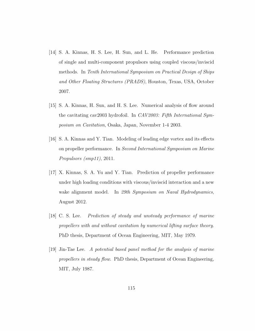
[14] S. A. Kinnas, H. S. Lee, H. Sun, and L. He. Performance prediction
of single and multi-component propulsors using coupled viscous/inviscid
methods. In Tenth International Symposium on Practical Design of Ships
and Other Floating Structures (PRADS), Houston, Texas, USA, October
2007.
[15] S. A. Kinnas, H. Sun, and H. S. Lee. Numerical analysis of flow around
the cavitating cav2003 hydrofoil. In CAV2003: Fifth International Sym-
posium on Cavitation, Osaka, Japan, November 1-4 2003.
[16] S. A. Kinnas and Y. Tian. Modeling of leading edge vortex and its effects
on propeller performance. In Second International Symposium on Marine
Propulsors (smp11), 2011.
[17] X. Kinnas, S. A. Yu and Y. Tian. Prediction of propeller performance
under high loading conditions with viscous/inviscid interaction and a new
wake alignment model. In 29th Symposium on Naval Hydrodynamics,
August 2012.
[18] C. S. Lee. Prediction of steady and unsteady performance of marine
propellers with and without cavitation by numerical lifting surface theory.
PhD thesis, Department of Ocean Engineering, MIT, May 1979.
[19] Jin-Tae Lee. A potential based panel method for the analysis of marine
propellers in steady flow. PhD thesis, Department of Ocean Engineering,
MIT, July 1987.
115

[20] W. M. Milewski. Three-dimensional viscous flow computations using
the integral boundary integral equations simultaneously coupled with a low
order panel method. PhD thesis, Department of Ocean Engineering, MIT,
1997.
[21] B. H. Mughal. A calculation method for the three dimensional boundary
layer equations in integral form. Master’s thesis, Department of Aero-
nautics and Astronautics, MIT, September 1992.
[22] B. H. Mughal. Integral Methods for Three Dimensional Boundary Layers.
PhD thesis, Department of Aeronautics and Astronautics, MIT, February
1998.
[23] B. Nishida and M. Drela. Fully simultaneous coupling for three dimen-
sional viscous/inviscid flows. In AIAA 13th Applied Aerodynamics Con-
ference, June 1995. 95-1806-CP.
[24] B. A. Nishida. Fully Simultaneous Coupling of the Full Potential Equa-
tion and the Integral Boundary Layer Equations in Three Dimensions.
PhD thesis, Department of Aeronautics and Astronautics, MIT, Febru-
ary 1996.
[25] Y. Pan. A viscous/inviscid interactive approach and its application to
wetted or cavitating hydrofoils and propellers with non-zero trailing edge
thickness. Master’s thesis, The Unversity of Texas at Austin, 2009.
116

[26] Y. Pan and S. A. Kinnas. A viscous/inviscid interactive approach for
the prediction of performance of hydrofoils and propellers with nonzero
trailing edge thickness. Journal of Ship Reasearch, vol 55(1):45–63, 2011.
[27] H. Schlichting. Boundary Layer Theory. McGraw-Hill, Inc., 1979.
[28] A. Sharma. Numerical modeling of a hydrofoil or a marine propeller
undergoing unsteady motion via a panel method and rans. Master’s
thesis, The Unversity of Texas at Austin, 2011.
[29] H. Sun. Performance Prediction of Cavitating Propulsors Using a Vis-
cous/Inviscid Interaction Method. PhD thesis, The Unversity of Texas at
Austin, 2008.
[30] F. M. White. Viscous Fluid Flow. McGraw-Hill, Inc., 1974.
117

Vita
Xiangming Yu was born in Shenyang, Liaoning Province, China on
22 March 1987, the son of Xiaosheng Yu and Guixia Liu. He received the
degree of Bachelor of Science in Engineering from the department of Naval
Architecture and Ocean Engineering, Shanghai Jiao Tong University, in July,
2010. In the fall of 2010, he enrolled at the University of Texas at Austin for
graduate studies in the Ocean Engineering Group of the Department of Civil,
Architectural and Environmental Engineering.
Permanent address: Tiexi District, East Shenliao Road,Unit 47-3, apt 241Shenyang City, Liaoning Province 110000People’s Republic of China
This thesis was typeset with LATEX† by the author.
†LATEX is a document preparation system developed by Leslie Lamport as a specialversion of Donald Knuth’s TEX Program.
118
Recommended