Nonsmooth Optimization for Statistical Learningwith Structured Matrix Regularization
PhD defense ofFederico Pierucci
Thesis supervised by
Prof. Zaid HarchaouiProf. Anatoli Juditsky
Dr. Jérôme Malick
Université Grenoble AlpesInria - Thoth and BiPoP
Inria GrenobleJune 23rd, 2017
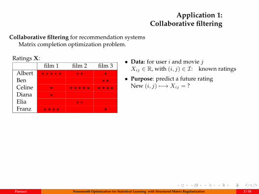
Application 1:Collaborative filtering
Collaborative filtering for recommendation systemsMatrix completion optimization problem.
Ratings X:film 1 film 2 film 3
Albert ? ? ? ? ? ? ? ?Ben ? ?Celine ? ? ? ? ? ? ? ? ? ?Diana ?Elia ? ?Franz ? ? ? ? ?
• Data: for user i and movie jXij ∈ R, with (i, j) ∈ I: known ratings
• Purpose: predict a future ratingNew (i, j) 7−→ Xij = ?
Low rank assumption:Movies can be divided into asmall number of types
For example:
minW∈Rd×k
1N
∑(i,j)∈I
|Wij −Xij | + λ ‖W‖σ,1
‖W‖σ,1 Nuclear norm = sum of singular values• convex function• surrogate of rank
Pierucci Nonsmooth Optimization for Statistical Learning with Structured Matrix Regularization 2 / 33
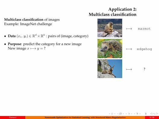
Application 2:Multiclass classification
Multiclass classification of imagesExample: ImageNet challenge
• Data (xi, yi) ∈ Rd×Rk : pairs of (image, category)
• Purpose: predict the category for a new imageNew image x 7−→ y = ?
7−→ marmot
7−→ edgehog
7−→ ?
minW∈Rd×k
1N
N∑i=1
max
0, 1 + maxr s.t. r 6=yi
W>r xi −W>
yixi
︸ ︷︷ ︸‖(Ax,yW)+‖∞
+ λ ‖W‖σ,1
Wj ∈ Rd : the j-th column of W
Pierucci Nonsmooth Optimization for Statistical Learning with Structured Matrix Regularization 3 / 33
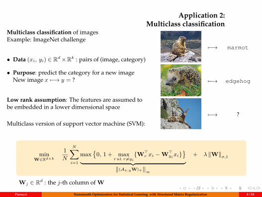
Application 2:Multiclass classification
Multiclass classification of imagesExample: ImageNet challenge
• Data (xi, yi) ∈ Rd×Rk : pairs of (image, category)
• Purpose: predict the category for a new imageNew image x 7−→ y = ?
Low rank assumption: The features are assumed tobe embedded in a lower dimensional space
Multiclass version of support vector machine (SVM):
7−→ marmot
7−→ edgehog
7−→ ?
minW∈Rd×k
1N
N∑i=1
max
0, 1 + maxr s.t. r 6=yi
W>r xi −W>
yixi
︸ ︷︷ ︸‖(Ax,yW)+‖∞
+ λ ‖W‖σ,1
Wj ∈ Rd : the j-th column of W
Pierucci Nonsmooth Optimization for Statistical Learning with Structured Matrix Regularization 3 / 33
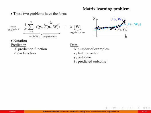
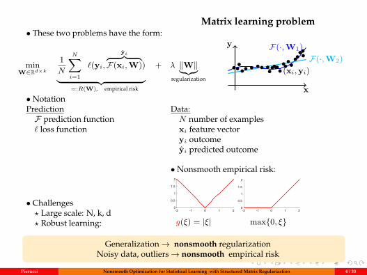
Matrix learning problem• These two problems have the form:
minW∈Rd×k
1N
N∑i=1
`(yi,yi︷ ︸︸ ︷
F(xi,W))︸ ︷︷ ︸=:R(W), empirical risk
+ λ ‖W‖︸︷︷︸regularization
x
y F(·,W1)F(·,W2)
••••• • •• •••••••(xi,yi)•••••••••
• NotationPredictionF prediction function` loss function
Data:N number of examplesxi feature vectoryi outcomeyi predicted outcome
• Challenges? Large scale: N, k, d? Robust learning:
• Nonsmooth empirical risk:
-2 -1 0 1 20
0.5
1
1.5
2
-2 -1 0 1 20
0.5
1
1.5
2
g(ξ) = |ξ| max0, ξ
Generalization→ nonsmooth regularizationNoisy data, outliers→ nonsmooth empirical risk
Pierucci Nonsmooth Optimization for Statistical Learning with Structured Matrix Regularization 4 / 33

My thesisin one slide
minW︸︷︷︸
2nd contribution
1N
N∑i=1
`(yi,F(xi,W))︸ ︷︷ ︸1st contribution
+ λ ‖W‖︸︷︷︸3rd contribution
1 - Smoothing techniques2 - Conditional gradient algorithms3 - Group nuclear norm
Pierucci Nonsmooth Optimization for Statistical Learning with Structured Matrix Regularization 5 / 33
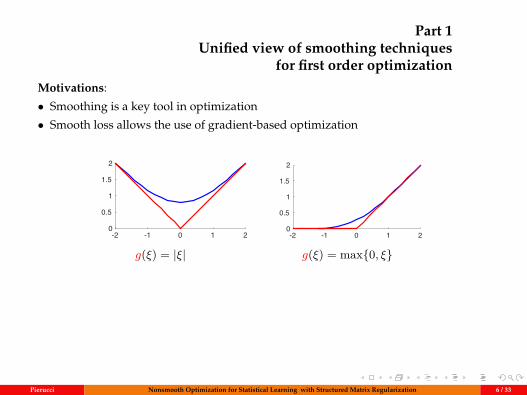
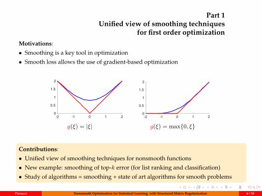
Part 1Unified view of smoothing techniques
for first order optimizationMotivations:
• Smoothing is a key tool in optimization
• Smooth loss allows the use of gradient-based optimization
-2 -1 0 1 20
0.5
1
1.5
2
-2 -1 0 1 20
0.5
1
1.5
2
g(ξ) = |ξ| g(ξ) = max0, ξ
Contributions:
• Unified view of smoothing techniques for nonsmooth functions
• New example: smoothing of top-k error (for list ranking and classification)
• Study of algorithms = smoothing + state of art algorithms for smooth problems
Pierucci Nonsmooth Optimization for Statistical Learning with Structured Matrix Regularization 6 / 33
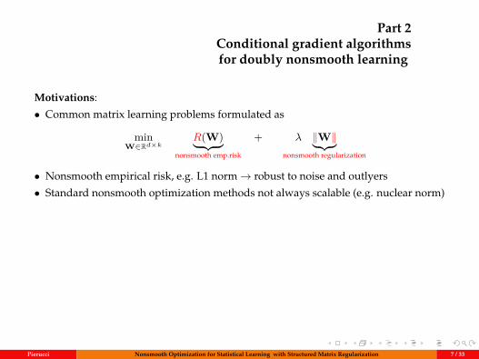
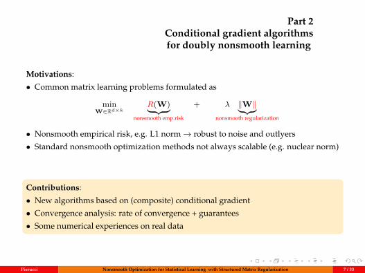
Part 2Conditional gradient algorithmsfor doubly nonsmooth learning
Motivations:
• Common matrix learning problems formulated as
minW∈Rd×k
R(W)︸ ︷︷ ︸nonsmooth emp.risk
+ λ ‖W‖︸︷︷︸nonsmooth regularization
• Nonsmooth empirical risk, e.g. L1 norm→ robust to noise and outlyers
• Standard nonsmooth optimization methods not always scalable (e.g. nuclear norm)
Contributions:
• New algorithms based on (composite) conditional gradient
• Convergence analysis: rate of convergence + guarantees
• Some numerical experiences on real data
Pierucci Nonsmooth Optimization for Statistical Learning with Structured Matrix Regularization 7 / 33
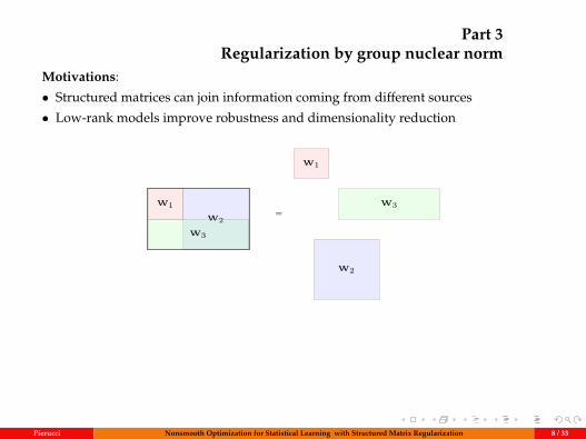
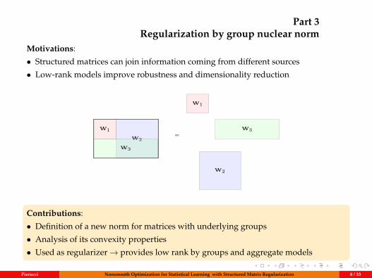
Part 3Regularization by group nuclear norm
Motivations:
• Structured matrices can join information coming from different sources
• Low-rank models improve robustness and dimensionality reduction
W1
W2
W3
W2
W3
W1=
Contributions:
• Definition of a new norm for matrices with underlying groups
• Analysis of its convexity properties
• Used as regularizer→ provides low rank by groups and aggregate models
Pierucci Nonsmooth Optimization for Statistical Learning with Structured Matrix Regularization 8 / 33
Outline
1 Unified view of smoothing techniques
2 Conditional gradient algorithms for doubly nonsmooth learning
3 Regularization by group nuclear norm
4 Conclusion and perspectives
Pierucci Nonsmooth Optimization for Statistical Learning with Structured Matrix Regularization 9 / 33
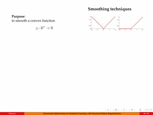
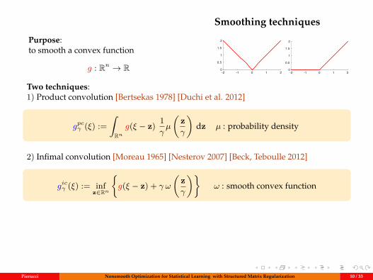
Smoothing techniques
Purpose:to smooth a convex function
g : Rn → R-2 -1 0 1 20
0.5
1
1.5
2
-2 -1 0 1 20
0.5
1
1.5
2
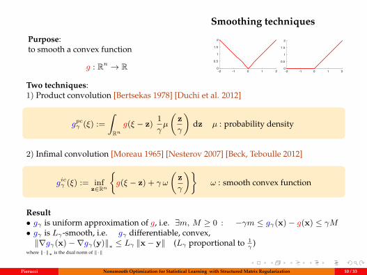
Two techniques:1) Product convolution [Bertsekas 1978] [Duchi et al. 2012]
gpcγ (ξ) :=∫Rn
g(ξ − z) 1γµ
(zγ
)dz µ : probability density
2) Infimal convolution [Moreau 1965] [Nesterov 2007] [Beck, Teboulle 2012]
gicγ (ξ) := infz∈Rn
g(ξ − z) + γ ω
(zγ
)ω : smooth convex function
Result• gγ is uniform approximation of g, i.e. ∃m, M ≥ 0 : −γm ≤ gγ(x)− g(x) ≤ γM• gγ is Lγ-smooth, i.e. gγ differentiable, convex,‖∇gγ(x)−∇gγ(y)‖∗ ≤ Lγ ‖x− y‖ (Lγ proportional to 1
γ)
where ‖·‖∗ is the dual norm of ‖·‖
Pierucci Nonsmooth Optimization for Statistical Learning with Structured Matrix Regularization 10 / 33
Smoothing techniques
Purpose:to smooth a convex function
g : Rn → R-2 -1 0 1 20
0.5
1
1.5
2
-2 -1 0 1 20
0.5
1
1.5
2
Two techniques:1) Product convolution [Bertsekas 1978] [Duchi et al. 2012]
gpcγ (ξ) :=∫Rn
g(ξ − z) 1γµ
(zγ
)dz µ : probability density
2) Infimal convolution [Moreau 1965] [Nesterov 2007] [Beck, Teboulle 2012]
gicγ (ξ) := infz∈Rn
g(ξ − z) + γ ω
(zγ
)ω : smooth convex function
Result• gγ is uniform approximation of g, i.e. ∃m, M ≥ 0 : −γm ≤ gγ(x)− g(x) ≤ γM• gγ is Lγ-smooth, i.e. gγ differentiable, convex,‖∇gγ(x)−∇gγ(y)‖∗ ≤ Lγ ‖x− y‖ (Lγ proportional to 1
γ)
where ‖·‖∗ is the dual norm of ‖·‖
Pierucci Nonsmooth Optimization for Statistical Learning with Structured Matrix Regularization 10 / 33
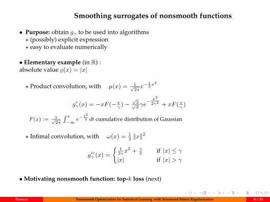
Smoothing surrogates of nonsmooth functions
• Purpose: obtain gγ to be used into algorithms? (possibly) explicit expression? easy to evaluate numerically
• Elementary example (in R) :absolute value g(x) = |x|
? Product convolution, with µ(x) = 1√2π e− 1
2x2
gcγ(x) = −xF (− xγ
)−√
2√πγe− x2
2γ2 + xF (xγ
)
F (x) := 1√2π
∫ x−∞ e−
t22 dt cumulative distribution of Gaussian
? Infimal convolution, with ω(x) = 12 ‖x‖
2
gicγ (x) = 1
2γ x2 + γ
2 if |x| ≤ γ|x| if |x| > γ
•Motivating nonsmooth function: top-k loss (next)
Pierucci Nonsmooth Optimization for Statistical Learning with Structured Matrix Regularization 11 / 33
Motivating nonsmooth functions: top-k lossExample: top-3 loss
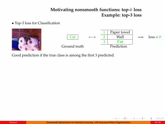
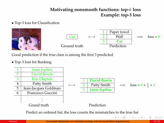
• Top-3 loss for Classification
Cat ←→1 Paper towel2 Wall3 Cat
=⇒ loss = 0
Ground truth Prediction
Good prediction if the true class is among the first 3 predicted.
• Top-3 loss for Ranking
1 Janis Joplins2 David Bowie3 Eric Clapton4 Patty Smith5 Jean-Jacques Goldman6 Francesco Guccini
...
←→1 David Bowie2 Patty Smith3 Janis Joplins
=⇒ loss = 0 + 13 + 0
Grund truth Prediction
Predict an ordered list, the loss counts the mismatches to the true list
Pierucci Nonsmooth Optimization for Statistical Learning with Structured Matrix Regularization 12 / 33
Motivating nonsmooth functions: top-k lossExample: top-3 loss
• Top-3 loss for Classification
Cat ←→1 Paper towel2 Wall3 Cat
=⇒ loss = 0
Ground truth Prediction
Good prediction if the true class is among the first 3 predicted.
• Top-3 loss for Ranking
1 Janis Joplins2 David Bowie3 Eric Clapton4 Patty Smith5 Jean-Jacques Goldman6 Francesco Guccini
...
←→1 David Bowie2 Patty Smith3 Janis Joplins
=⇒ loss = 0 + 13 + 0
Grund truth Prediction
Predict an ordered list, the loss counts the mismatches to the true list
Pierucci Nonsmooth Optimization for Statistical Learning with Structured Matrix Regularization 12 / 33
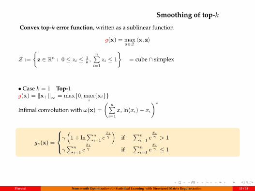
Smoothing of top-k
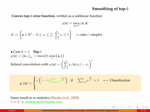
Convex top-k error function, written as a sublinear function
g(x) = maxz∈Z〈x, z〉
Z :=
z ∈ Rn : 0 ≤ zi ≤ 1k,n∑i=1
zi ≤ 1
= cube ∩ simplex
• Case k = 1 Top-1g(x) = ‖x+‖∞ = max0,max
ixi
Infimal convolution with ω(x) =(
n∑i=1
xi ln(xi)− xi)∗
gγ(x) =
γ(
1 + ln∑n
i=1 exiγ
)if
∑n
i=1 exiγ > 1
γ∑n
i=1 exiγ if
∑n
i=1 exiγ ≤ 1
xx
Pierucci Nonsmooth Optimization for Statistical Learning with Structured Matrix Regularization 13 / 33
Smoothing of top-k
Convex top-k error function, written as a sublinear function
g(x) = maxz∈Z〈x, z〉
Z :=
z ∈ Rn : 0 ≤ zi ≤ 1k,n∑i=1
zi ≤ 1
= cube ∩ simplex
• Case k = 1 Top-1g(x) = ‖x+‖∞ = max0,max
ixi
Infimal convolution with ω(x) =(
n∑i=1
xi ln(xi)− xi)∗
gγ(x) =
γ(
1 + ln∑n
i=1 exiγ
)if
∑n
i=1 exiγ > 1 ←− Classification
Same result as in statistics [Hastie et al., 2008]γ = 1→ multinomial logistic loss
Pierucci Nonsmooth Optimization for Statistical Learning with Structured Matrix Regularization 13 / 33
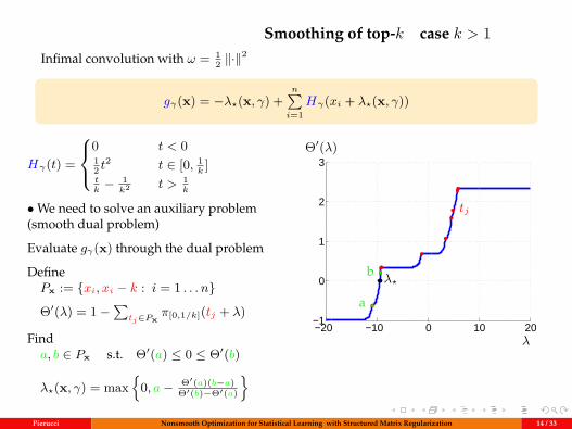
Smoothing of top-k case k > 1Infimal convolution with ω = 1
2 ‖·‖2
gγ(x) = −λ?(x, γ) +n∑i=1
Hγ(xi + λ?(x, γ))
Hγ(t) =
0 t < 012 t
2 t ∈ [0, 1k
]tk− 1
k2 t > 1k
•We need to solve an auxiliary problem(smooth dual problem)
Evaluate gγ(x) through the dual problem
DefinePx := xi, xi − k : i = 1 . . . n
Θ′(λ) = 1−∑
tj∈Pxπ[0,1/k](tj + λ)
Finda, b ∈ Px s.t. Θ′(a) ≤ 0 ≤ Θ′(b)
λ?(x, γ) = max
0, a− Θ′(a)(b−a)Θ′(b)−Θ′(a)
−20 −10 0 10 20−1
0
1
2
3∇Θ (λ)Θ′(λ)
λ
λ?b
a
tj
Pierucci Nonsmooth Optimization for Statistical Learning with Structured Matrix Regularization 14 / 33
Outline
1 Unified view of smoothing techniques
2 Conditional gradient algorithms for doubly nonsmooth learning
3 Regularization by group nuclear norm
4 Conclusion and perspectives
Pierucci Nonsmooth Optimization for Statistical Learning with Structured Matrix Regularization 15 / 33
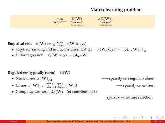
Matrix learning problem
minW∈Rd×k
R(W)︸ ︷︷ ︸nonsmooth
+ λΩ(W)︸ ︷︷ ︸nonsmooth
Empirical risk R(W) := 1N
∑N
i=1 `(W,xi,yi)• Top-k for ranking and multiclass classification `1(W,x,y) := ‖(Ax,yW)+‖∞• L1 for regression `1(W,x,y) := |Ax,yW|
Regularizer (typically norm) Ω(W)• Nuclear norm ‖W‖σ,1 −→ sparsity on singular values
• L1 norm ‖W‖1 :=∑d
i=1
∑k
j=1 |Wij | −→ sparsity on entries
• Group nuclear norm ΩG(W) (of contribution 3)
sparsity↔ feature selection
Pierucci Nonsmooth Optimization for Statistical Learning with Structured Matrix Regularization 16 / 33

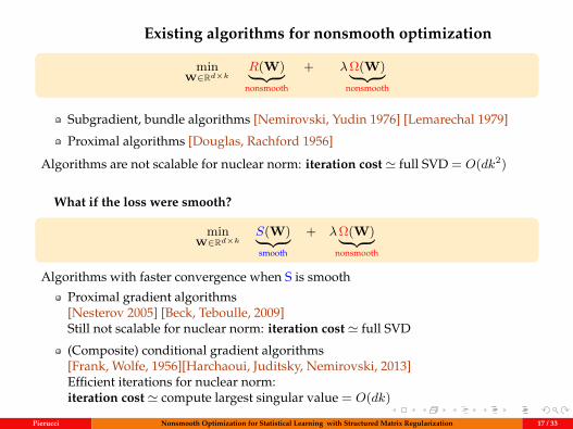
Existing algorithms for nonsmooth optimization
minW∈Rd×k
R(W)︸ ︷︷ ︸nonsmooth
+ λΩ(W)︸ ︷︷ ︸nonsmooth
Subgradient, bundle algorithms [Nemirovski, Yudin 1976] [Lemarechal 1979]
Proximal algorithms [Douglas, Rachford 1956]
Algorithms are not scalable for nuclear norm: iteration cost ' full SVD = O(dk2)
What if the loss were smooth?
minW∈Rd×k
S(W)︸ ︷︷ ︸smooth
+ λΩ(W)︸ ︷︷ ︸nonsmooth
Algorithms with faster convergence when S is smooth
Proximal gradient algorithms[Nesterov 2005] [Beck, Teboulle, 2009]Still not scalable for nuclear norm: iteration cost ' full SVD
(Composite) conditional gradient algorithms[Frank, Wolfe, 1956][Harchaoui, Juditsky, Nemirovski, 2013]Efficient iterations for nuclear norm:iteration cost ' compute largest singular value = O(dk)
Pierucci Nonsmooth Optimization for Statistical Learning with Structured Matrix Regularization 17 / 33
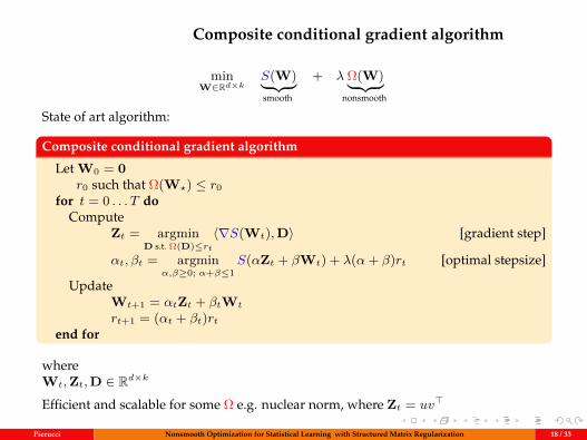
Composite conditional gradient algorithm
minW∈Rd×k
S(W)︸ ︷︷ ︸smooth
+ λ Ω(W)︸ ︷︷ ︸nonsmooth
State of art algorithm:
Composite conditional gradient algorithm
Let W0 = 0r0 such that Ω(W?) ≤ r0
for t = 0 . . . T doCompute
Zt = argminD s.t. Ω(D)≤rt
〈∇S(Wt),D〉 [gradient step]
αt, βt = argminα,β≥0; α+β≤1
S(αZt + βWt) + λ(α+ β)rt [optimal stepsize]
UpdateWt+1 = αtZt + βtWt
rt+1 = (αt + βt)rtend for
whereWt,Zt,D ∈ Rd×k
Efficient and scalable for some Ω e.g. nuclear norm, where Zt = uv>
Pierucci Nonsmooth Optimization for Statistical Learning with Structured Matrix Regularization 18 / 33
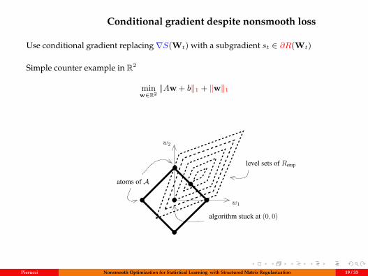
Conditional gradient despite nonsmooth loss
Use conditional gradient replacing∇S(Wt) with a subgradient st ∈ ∂R(Wt)
Simple counter example in R2
minw∈R2
‖Aw + b‖1 + ‖w‖1
4 Federico Pierucci et al.
Algorithm 1 Composite Conditional GradientInputs: , Initialize W0 = 0, t = 1for k = 0 . . . K do
Call the linear minimization oracle: LMO(Wk)Compute
min1,...,t0
tX
i=1
i + R
tX
i=1
iai
!
Increment t t + 1end forReturn W =
Pi iai
Algorithm 2 Conditional gradient algorithm: Frank-WolfeInputInitialize W0 = 0, t = 1for k = 0 . . . K do
Call linear minimization oracle adaptiveak LMO(Wt)Set step-size ↵k = 2/(2 + k)Update Wk+1 (1 ↵k)Wk + ↵kak
end forReturn WK
2.3 How about nonsmooth empirical risk?
Composite conditional gradient assumes that the empirical risk in the objective function g is smooth.Indeed, at each iteration, the algorithm requires to computerR(W ). Should we consider nonsmooth lossfunctions, such as the `1-loss or the hinge-loss, the convergence of the algorithm is unclear if we replacethe gradient by a subgradient in @R(W ). In fact, we can produce a simple counterexample showing thatthe corresponding algorithm can get stuck in a suboptimal point.
Let us describe and draw in Figure 1 a counterexample in two dimensions (generalization to higher di-mension is straightforward). We consider the `1-norm with its four atoms (1, 0), (0, 1), (1, 0), (0,1)and a convex function of the type of a translated weighted `1-norm
f(w1, w2) = |w1 + w2 3/2| + 4 |w2 w1| .
level sets of Remp
w1
w2
atoms of A
algorithm stuck at (0, 0)
Fig. 1 Drawing of a situation where the algorithm using a subgradient of a nonsmooth empirical risk does not converge.
We observe that the four directions given by the atoms go from (0, 0) towards level-sets of R withlarger values. This yields that, for small , the minimization of the objective function on these directions
Pierucci Nonsmooth Optimization for Statistical Learning with Structured Matrix Regularization 19 / 33
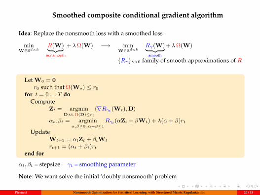
Smoothed composite conditional gradient algorithm
Idea: Replace the nonsmooth loss with a smoothed loss
minW∈Rd×k
R(W)︸ ︷︷ ︸nonsmooth
+λΩ(W) −→ minW∈Rd×k
Rγ(W)︸ ︷︷ ︸smooth
+λΩ(W)
Rγγ>0 family of smooth approximations of R
Let W0 = 0r0 such that Ω(W?) ≤ r0
for t = 0 . . . T doCompute
Zt = argminD s.t. Ω(D)≤rt
〈∇Rγt (Wt),D〉
αt, βt = argminα,β≥0; α+β≤1
Rγt (αZt + βWt) + λ(α+ β)rt
UpdateWt+1 = αtZt + βtWt
rt+1 = (αt + βt)rtend for
αt, βt = stepsize γt = smoothing parameter
Note: We want solve the initial ‘doubly nonsmooth’ problem
Pierucci Nonsmooth Optimization for Statistical Learning with Structured Matrix Regularization 20 / 33
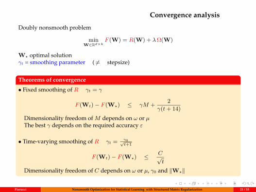
Convergence analysis
Doubly nonsmooth problem
minW∈Rd×k
F (W) = R(W) + λΩ(W)
W? optimal solutionγt = smoothing parameter ( 6= stepsize)
Theorems of convergence
• Fixed smoothing of R γt = γ
F (Wt)− F (W?) ≤ γM + 2γ(t+ 14)
Dimensionality freedom of M depends on ω or µThe best γ depends on the required accuracy ε
• Time-varying smoothing of R γt = γ0√t+1
F (Wt)− F (W?) ≤ C√t
Dimensionality freedom of C depends on ω or µ, γ0 and ‖W?‖
Pierucci Nonsmooth Optimization for Statistical Learning with Structured Matrix Regularization 21 / 33
Algoritm implementation
PackageAll the Matlab code written from scratch, in particular:
• Multiclass SVM
• Top-k multiclass SVM
• All other smoothed functions
MemoryEfficient memory management
• Tools to operate with low rank variables
• Tools to work with sparse sub-matrices of low rank matrices (collaborative filtering)
Numerical experiments - 2 motivating applications
• Fix smoothing - matrix completion (regression)
• Time-varying smoothing - top-5 multiclass classification
Pierucci Nonsmooth Optimization for Statistical Learning with Structured Matrix Regularization 22 / 33
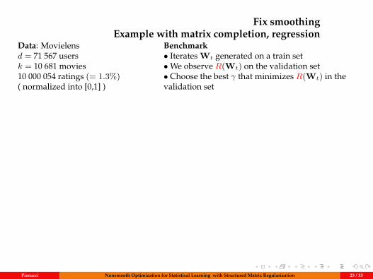
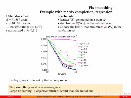
Fix smoothingExample with matrix completion, regression
Data: Movielensd = 71 567 usersk = 10 681 movies10 000 054 ratings (= 1.3%)( normalized into [0,1] )
Benchmark• Iterates Wt generated on a train set•We observe R(Wt) on the validation set• Choose the best γ that minimizes R(Wt) in thevalidation set
100
1020.188
0.2457
0.3211
0.4196
0.5484
0.7167
iterations
Emp. risk on validation set, λ=10−6
γ = 0.001γ = 0.01γ = 0.1γ = 0.5γ = 1γ = 5γ = 10γ = 50γ = best
Each γ gives a different optimization problem
Tiny smoothing→ slower convergenceLarge smoothing→ objective much different than the initial one
Pierucci Nonsmooth Optimization for Statistical Learning with Structured Matrix Regularization 23 / 33
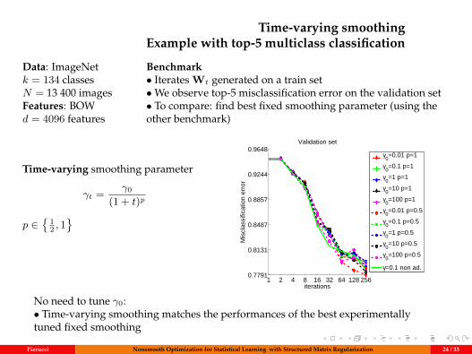
Time-varying smoothingExample with top-5 multiclass classification
Data: ImageNetk = 134 classesN = 13 400 imagesFeatures: BOWd = 4096 features
Benchmark• Iterates Wt generated on a train set•We observe top-5 misclassification error on the validation set• To compare: find best fixed smoothing parameter (using theother benchmark)
Time-varying smoothing parameter
γt = γ0
(1 + t)p
p ∈
12 , 1
1 2 4 8 16 32 64 128 2560.7791
0.8131
0.8487
0.8857
0.9244
0.9648Validation set
iterations
Mis
clas
sific
atio
n er
ror
γ0=0.01 p=1
γ0=0.1 p=1
γ0=1 p=1
γ0=10 p=1
γ0=100 p=1
γ0=0.01 p=0.5
γ0=0.1 p=0.5
γ0=1 p=0.5
γ0=10 p=0.5
γ0=100 p=0.5
γ=0.1 non ad.
No need to tune γ0:• Time-varying smoothing matches the performances of the best experimentallytuned fixed smoothing
Pierucci Nonsmooth Optimization for Statistical Learning with Structured Matrix Regularization 24 / 33
Outline
1 Unified view of smoothing techniques
2 Conditional gradient algorithms for doubly nonsmooth learning
3 Regularization by group nuclear norm
4 Conclusion and perspectives
Pierucci Nonsmooth Optimization for Statistical Learning with Structured Matrix Regularization 25 / 33

Group nuclear norm
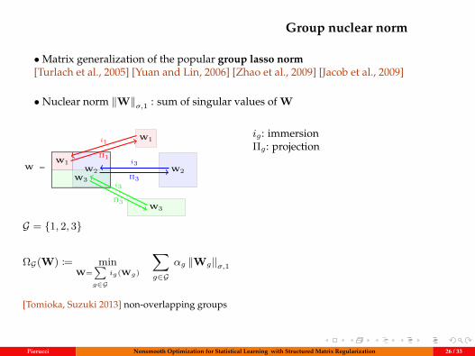
•Matrix generalization of the popular group lasso norm[Turlach et al., 2005] [Yuan and Lin, 2006] [Zhao et al., 2009] [Jacob et al., 2009]
• Nuclear norm ‖W‖σ,1 : sum of singular values of W
W1
W2
W3
W2W3
W1W =
i1
Π1
i3
Π3
i3
Π3
G = 1, 2, 3
ΩG(W) := minW=∑g∈G
ig(Wg)
∑g∈G
αg ‖Wg‖σ,1
[Tomioka, Suzuki 2013] non-overlapping groups
ig : immersionΠg : projection
Convex analysis - theoretical study
• Fenchel conjugate Ω∗G• Dual norm ΩG• Expression of ΩG as a support function
• Convex hull of functions involving rank
Pierucci Nonsmooth Optimization for Statistical Learning with Structured Matrix Regularization 26 / 33
Group nuclear norm
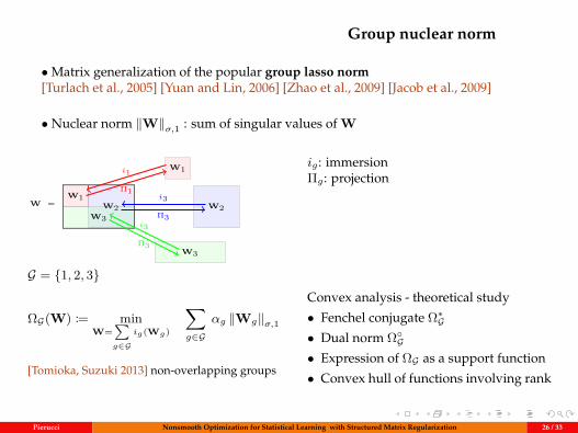
•Matrix generalization of the popular group lasso norm[Turlach et al., 2005] [Yuan and Lin, 2006] [Zhao et al., 2009] [Jacob et al., 2009]
• Nuclear norm ‖W‖σ,1 : sum of singular values of W
W1
W2
W3
W2W3
W1W =
i1
Π1
i3
Π3
i3
Π3
G = 1, 2, 3
ΩG(W) := minW=∑g∈G
ig(Wg)
∑g∈G
αg ‖Wg‖σ,1
[Tomioka, Suzuki 2013] non-overlapping groups
ig : immersionΠg : projection
Convex analysis - theoretical study
• Fenchel conjugate Ω∗G• Dual norm ΩG• Expression of ΩG as a support function
• Convex hull of functions involving rank
Pierucci Nonsmooth Optimization for Statistical Learning with Structured Matrix Regularization 26 / 33
Group nuclear norm
•Matrix generalization of the popular group lasso norm[Turlach et al., 2005] [Yuan and Lin, 2006] [Zhao et al., 2009] [Jacob et al., 2009]
• Nuclear norm ‖W‖σ,1 : sum of singular values of W
W1
W2
W3
W2W3
W1W =
i1
Π1
i3
Π3
i3
Π3
G = 1, 2, 3
ΩG(W) := minW=∑g∈G
ig(Wg)
∑g∈G
αg ‖Wg‖σ,1
[Tomioka, Suzuki 2013] non-overlapping groups
ig : immersionΠg : projection
Convex analysis - theoretical study
• Fenchel conjugate Ω∗G• Dual norm ΩG• Expression of ΩG as a support function
• Convex hull of functions involving rank
Pierucci Nonsmooth Optimization for Statistical Learning with Structured Matrix Regularization 26 / 33
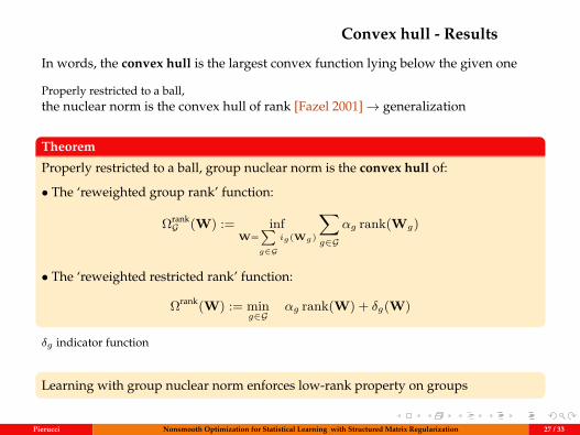
Convex hull - Results
In words, the convex hull is the largest convex function lying below the given one
Properly restricted to a ball,the nuclear norm is the convex hull of rank [Fazel 2001]→ generalization
Theorem
Properly restricted to a ball, group nuclear norm is the convex hull of:
• The ‘reweighted group rank’ function:
ΩrankG (W) := inf
W=∑g∈G
ig(Wg)
∑g∈G
αg rank(Wg)
• The ‘reweighted restricted rank’ function:
Ωrank(W) := ming∈G
αg rank(W) + δg(W)
δg indicator function
Learning with group nuclear norm enforces low-rank property on groups
Pierucci Nonsmooth Optimization for Statistical Learning with Structured Matrix Regularization 27 / 33

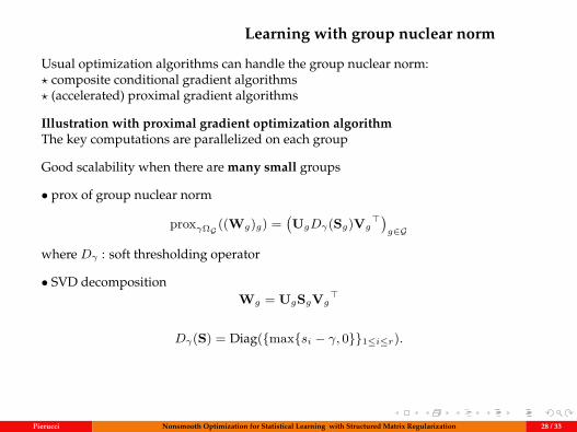
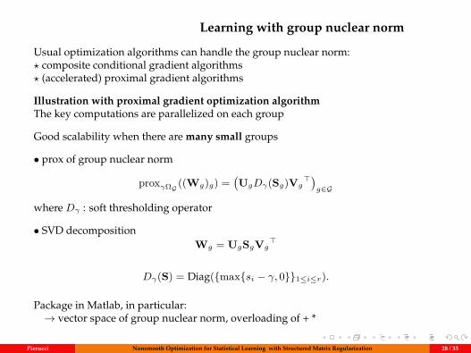
Learning with group nuclear norm
Usual optimization algorithms can handle the group nuclear norm:? composite conditional gradient algorithms? (accelerated) proximal gradient algorithms
Illustration with proximal gradient optimization algorithmThe key computations are parallelized on each group
Good scalability when there are many small groups
• prox of group nuclear norm
proxγΩG ((Wg)g) =(UgDγ(Sg)Vg
>)g∈G
where Dγ : soft thresholding operator
• SVD decompositionWg = UgSgVg
>
Dγ(S) = Diag(maxsi − γ, 01≤i≤r).
Package in Matlab, in particular:→ vector space of group nuclear norm, overloading of + *
Pierucci Nonsmooth Optimization for Statistical Learning with Structured Matrix Regularization 28 / 33
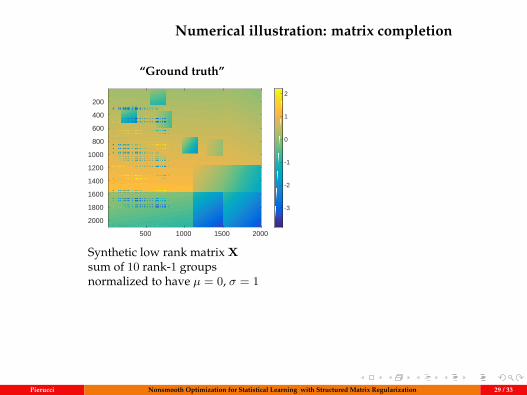
Numerical illustration: matrix completion
“Ground truth”data
500 1000 1500 2000
200
400
600
800
1000
1200
1400
1600
1800
2000
-3
-2
-1
0
1
2
Synthetic low rank matrix Xsum of 10 rank-1 groupsnormalized to have µ = 0, σ = 1
Pierucci Nonsmooth Optimization for Statistical Learning with Structured Matrix Regularization 29 / 33
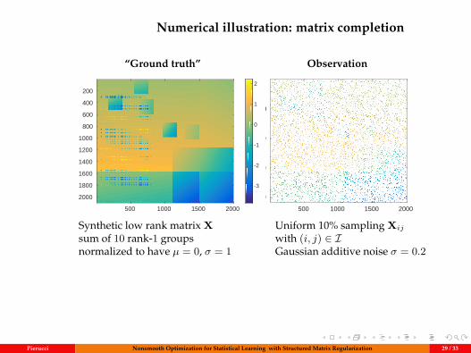
Numerical illustration: matrix completion
“Ground truth” Observationdata
500 1000 1500 2000
200
400
600
800
1000
1200
1400
1600
1800
2000
-3
-2
-1
0
1
2
observations
500 1000 1500 2000
500
1000
1500
2000
-3
-2
-1
0
1
2
Synthetic low rank matrix Xsum of 10 rank-1 groupsnormalized to have µ = 0, σ = 1
Uniform 10% sampling Xij
with (i, j) ∈ IGaussian additive noise σ = 0.2
Pierucci Nonsmooth Optimization for Statistical Learning with Structured Matrix Regularization 29 / 33
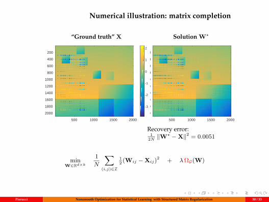
Numerical illustration: matrix completion
“Ground truth” X Solution W?
data
500 1000 1500 2000
200
400
600
800
1000
1200
1400
1600
1800
2000
-3
-2
-1
0
1
2
solution
500 1000 1500 2000
200
400
600
800
1000
1200
1400
1600
1800
2000
-3
-2
-1
0
1
2
Recovery error:1
2N ‖W? −X‖2 = 0.0051
minW∈Rd×k
1N
∑(i,j)∈I
12 (Wij −Xij)2 + λΩG(W)
Pierucci Nonsmooth Optimization for Statistical Learning with Structured Matrix Regularization 30 / 33
Outline
1 Unified view of smoothing techniques
2 Conditional gradient algorithms for doubly nonsmooth learning
3 Regularization by group nuclear norm
4 Conclusion and perspectives
Pierucci Nonsmooth Optimization for Statistical Learning with Structured Matrix Regularization 31 / 33
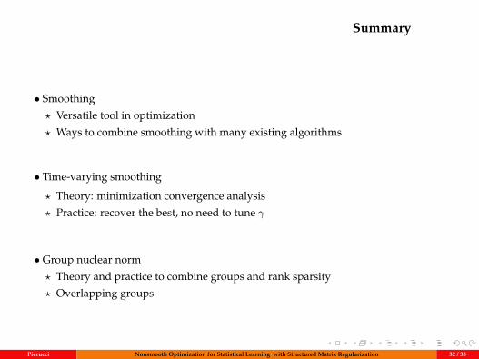
Summary
• Smoothing
? Versatile tool in optimization
? Ways to combine smoothing with many existing algorithms
• Time-varying smoothing
? Theory: minimization convergence analysis
? Practice: recover the best, no need to tune γ
• Group nuclear norm
? Theory and practice to combine groups and rank sparsity
? Overlapping groups
Pierucci Nonsmooth Optimization for Statistical Learning with Structured Matrix Regularization 32 / 33
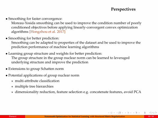
Perspectives
• Smoothing for faster convergence:Moreau-Yosida smoothing can be used to improve the condition number of poorlyconditioned objectives before applying linearly-convergent convex optimizationalgorithms [Hongzhou et al. 2017]
• Smoothing for better prediction:Smoothing can be adapted to properties of the dataset and be used to improve theprediction performance of machine learning algorithms
• Learning group structure and weights for better prediction:The group structure in the group nuclear norm can be learned to leveragedunderlying structure and improve the prediction
• Extensions to group Schatten norm
• Potential applications of group nuclear norm
? multi-attribute classification
? multiple tree hierarchies
? dimensionality reduction, feature selection e.g. concatenate features, avoid PCA
Thank You
Pierucci Nonsmooth Optimization for Statistical Learning with Structured Matrix Regularization 33 / 33
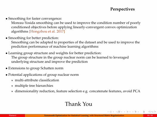
Recommended