Embed Size (px)
Citation preview
Nonsmooth Optimization for Statistical Learningwith Structured Matrix Regularization
PhD defense ofFederico Pierucci
Thesis supervised by
Prof. Zaid HarchaouiProf. Anatoli Juditsky
Dr. Jérôme Malick
Université Grenoble AlpesInria - Thoth and BiPoP
Inria GrenobleJune 23rd, 2017
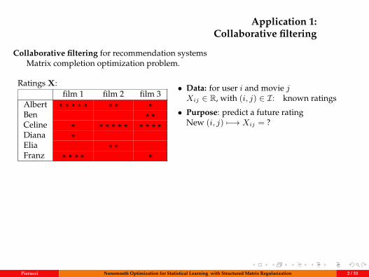
Application 1:Collaborative filtering
Collaborative filtering for recommendation systemsMatrix completion optimization problem.
Ratings X:film 1 film 2 film 3
Albert ? ? ? ? ? ? ? ?Ben ? ?Celine ? ? ? ? ? ? ? ? ? ?Diana ?Elia ? ?Franz ? ? ? ? ?
• Data: for user i and movie jXij ∈ R, with (i, j) ∈ I: known ratings
• Purpose: predict a future ratingNew (i, j) 7−→ Xij = ?
Low rank assumption:Movies can be divided into asmall number of types
For example:
minW∈Rd×k
1N
∑(i,j)∈I
|Wij −Xij | + λ ‖W‖σ,1
‖W‖σ,1 Nuclear norm = sum of singular values• convex function• surrogate of rank
Pierucci Nonsmooth Optimization for Statistical Learning with Structured Matrix Regularization 2 / 33
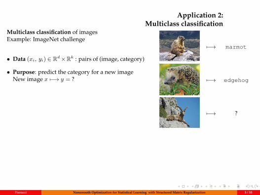
Application 2:Multiclass classification
Multiclass classification of imagesExample: ImageNet challenge
• Data (xi, yi) ∈ Rd×Rk : pairs of (image, category)
• Purpose: predict the category for a new imageNew image x 7−→ y = ?
7−→ marmot
7−→ edgehog
7−→ ?
minW∈Rd×k
1N
N∑i=1
max
0, 1 + maxr s.t. r 6=yi
W>r xi −W>
yixi
︸ ︷︷ ︸‖(Ax,yW)+‖∞
+ λ ‖W‖σ,1
Wj ∈ Rd : the j-th column of W
Pierucci Nonsmooth Optimization for Statistical Learning with Structured Matrix Regularization 3 / 33
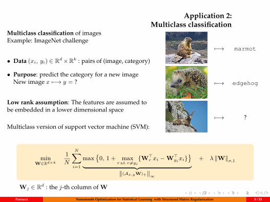
Application 2:Multiclass classification
Multiclass classification of imagesExample: ImageNet challenge
• Data (xi, yi) ∈ Rd×Rk : pairs of (image, category)
• Purpose: predict the category for a new imageNew image x 7−→ y = ?
Low rank assumption: The features are assumed tobe embedded in a lower dimensional space
Multiclass version of support vector machine (SVM):
7−→ marmot
7−→ edgehog
7−→ ?
minW∈Rd×k
1N
N∑i=1
max
0, 1 + maxr s.t. r 6=yi
W>r xi −W>
yixi
︸ ︷︷ ︸‖(Ax,yW)+‖∞
+ λ ‖W‖σ,1
Wj ∈ Rd : the j-th column of W
Pierucci Nonsmooth Optimization for Statistical Learning with Structured Matrix Regularization 3 / 33
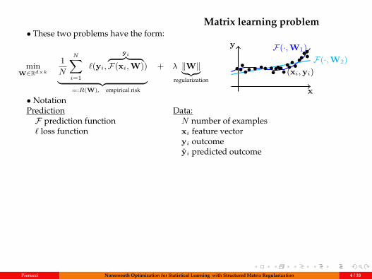
Matrix learning problem• These two problems have the form:
minW∈Rd×k
1N
N∑i=1
`(yi,yi︷ ︸︸ ︷
F(xi,W))︸ ︷︷ ︸=:R(W), empirical risk
+ λ ‖W‖︸︷︷︸regularization
x
y F(·,W1)F(·,W2)
••••• • •• •••••••(xi,yi)•••••••••
• NotationPredictionF prediction function` loss function
Data:N number of examplesxi feature vectoryi outcomeyi predicted outcome
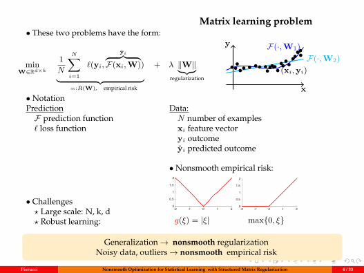
• Challenges? Large scale: N, k, d? Robust learning:
• Nonsmooth empirical risk:
-2 -1 0 1 20
0.5
1
1.5
2
-2 -1 0 1 20
0.5
1
1.5
2
g(ξ) = |ξ| max0, ξ
Generalization→ nonsmooth regularizationNoisy data, outliers→ nonsmooth empirical risk
Pierucci Nonsmooth Optimization for Statistical Learning with Structured Matrix Regularization 4 / 33
Matrix learning problem• These two problems have the form:
minW∈Rd×k
1N
N∑i=1
`(yi,yi︷ ︸︸ ︷
F(xi,W))︸ ︷︷ ︸=:R(W), empirical risk
+ λ ‖W‖︸︷︷︸regularization
x
y F(·,W1)F(·,W2)
••••• • •• •••••••(xi,yi)•••••••••
• NotationPredictionF prediction function` loss function
Data:N number of examplesxi feature vectoryi outcomeyi predicted outcome
• Challenges? Large scale: N, k, d? Robust learning:
• Nonsmooth empirical risk:
-2 -1 0 1 20
0.5
1
1.5
2
-2 -1 0 1 20
0.5
1
1.5
2
g(ξ) = |ξ| max0, ξ
Generalization→ nonsmooth regularizationNoisy data, outliers→ nonsmooth empirical risk
Pierucci Nonsmooth Optimization for Statistical Learning with Structured Matrix Regularization 4 / 33

My thesisin one slide
minW︸︷︷︸
2nd contribution
1N
N∑i=1
`(yi,F(xi,W))︸ ︷︷ ︸1st contribution
+ λ ‖W‖︸︷︷︸3rd contribution
1 - Smoothing techniques2 - Conditional gradient algorithms3 - Group nuclear norm
Pierucci Nonsmooth Optimization for Statistical Learning with Structured Matrix Regularization 5 / 33
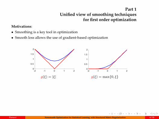
Part 1Unified view of smoothing techniques
for first order optimizationMotivations:
• Smoothing is a key tool in optimization
• Smooth loss allows the use of gradient-based optimization
-2 -1 0 1 20
0.5
1
1.5
2
-2 -1 0 1 20
0.5
1
1.5
2
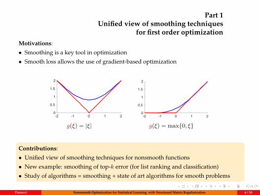
g(ξ) = |ξ| g(ξ) = max0, ξ
Contributions:
• Unified view of smoothing techniques for nonsmooth functions
• New example: smoothing of top-k error (for list ranking and classification)
• Study of algorithms = smoothing + state of art algorithms for smooth problems
Pierucci Nonsmooth Optimization for Statistical Learning with Structured Matrix Regularization 6 / 33
Part 1Unified view of smoothing techniques
for first order optimizationMotivations:
• Smoothing is a key tool in optimization
• Smooth loss allows the use of gradient-based optimization
-2 -1 0 1 20
0.5
1
1.5
2
-2 -1 0 1 20
0.5
1
1.5
2
g(ξ) = |ξ| g(ξ) = max0, ξ
Contributions:
• Unified view of smoothing techniques for nonsmooth functions
• New example: smoothing of top-k error (for list ranking and classification)
• Study of algorithms = smoothing + state of art algorithms for smooth problems
Pierucci Nonsmooth Optimization for Statistical Learning with Structured Matrix Regularization 6 / 33
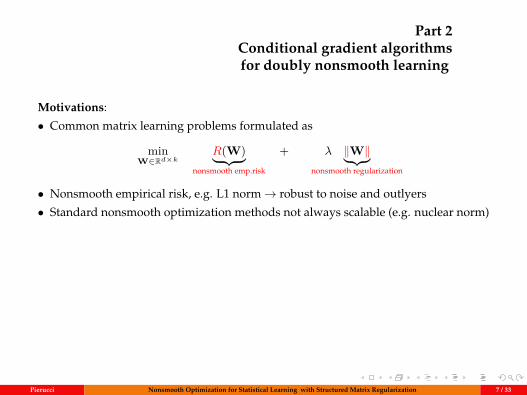
Part 2Conditional gradient algorithmsfor doubly nonsmooth learning
Motivations:
• Common matrix learning problems formulated as
minW∈Rd×k
R(W)︸ ︷︷ ︸nonsmooth emp.risk
+ λ ‖W‖︸︷︷︸nonsmooth regularization
• Nonsmooth empirical risk, e.g. L1 norm→ robust to noise and outlyers
• Standard nonsmooth optimization methods not always scalable (e.g. nuclear norm)
Contributions:
• New algorithms based on (composite) conditional gradient
• Convergence analysis: rate of convergence + guarantees
• Some numerical experiences on real data
Pierucci Nonsmooth Optimization for Statistical Learning with Structured Matrix Regularization 7 / 33
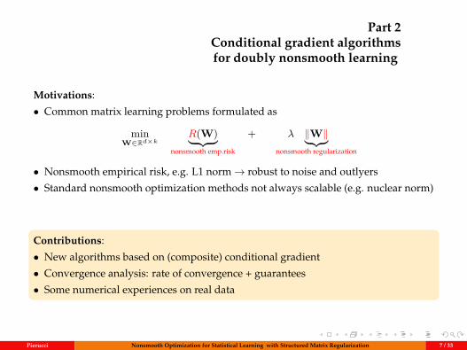
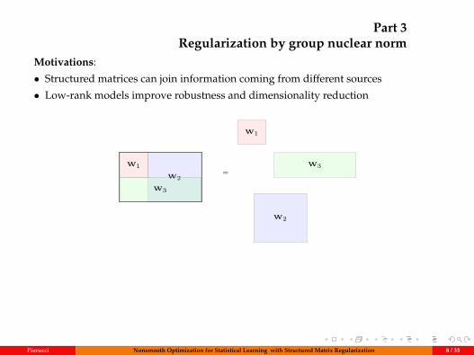
Part 3Regularization by group nuclear norm
Motivations:
• Structured matrices can join information coming from different sources
• Low-rank models improve robustness and dimensionality reduction
W1
W2
W3
W2
W3
W1=
Contributions:
• Definition of a new norm for matrices with underlying groups
• Analysis of its convexity properties
• Used as regularizer→ provides low rank by groups and aggregate models
Pierucci Nonsmooth Optimization for Statistical Learning with Structured Matrix Regularization 8 / 33
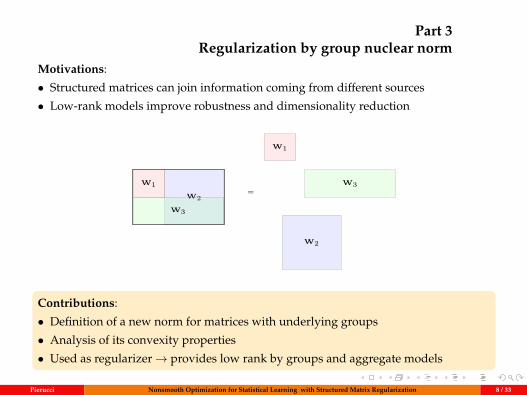
Outline
1 Unified view of smoothing techniques
2 Conditional gradient algorithms for doubly nonsmooth learning
3 Regularization by group nuclear norm
4 Conclusion and perspectives
Pierucci Nonsmooth Optimization for Statistical Learning with Structured Matrix Regularization 9 / 33
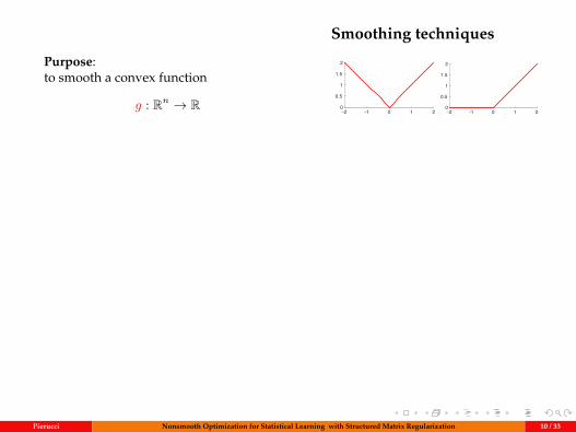
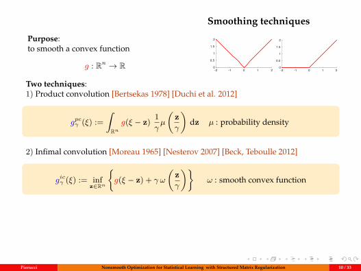
Smoothing techniques
Purpose:to smooth a convex function
g : Rn → R-2 -1 0 1 20
0.5
1
1.5
2
-2 -1 0 1 20
0.5
1
1.5
2
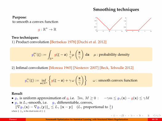
Two techniques:1) Product convolution [Bertsekas 1978] [Duchi et al. 2012]
gpcγ (ξ) :=∫Rn
g(ξ − z) 1γµ
(zγ
)dz µ : probability density
2) Infimal convolution [Moreau 1965] [Nesterov 2007] [Beck, Teboulle 2012]
gicγ (ξ) := infz∈Rn
g(ξ − z) + γ ω
(zγ
)ω : smooth convex function
Result• gγ is uniform approximation of g, i.e. ∃m, M ≥ 0 : −γm ≤ gγ(x)− g(x) ≤ γM• gγ is Lγ-smooth, i.e. gγ differentiable, convex,‖∇gγ(x)−∇gγ(y)‖∗ ≤ Lγ ‖x− y‖ (Lγ proportional to 1
γ)
where ‖·‖∗ is the dual norm of ‖·‖
Pierucci Nonsmooth Optimization for Statistical Learning with Structured Matrix Regularization 10 / 33
Smoothing techniques
Purpose:to smooth a convex function
g : Rn → R-2 -1 0 1 20
0.5
1
1.5
2
-2 -1 0 1 20
0.5
1
1.5
2
Two techniques:1) Product convolution [Bertsekas 1978] [Duchi et al. 2012]
gpcγ (ξ) :=∫Rn
g(ξ − z) 1γµ
(zγ
)dz µ : probability density
2) Infimal convolution [Moreau 1965] [Nesterov 2007] [Beck, Teboulle 2012]
gicγ (ξ) := infz∈Rn
g(ξ − z) + γ ω
(zγ
)ω : smooth convex function
Result• gγ is uniform approximation of g, i.e. ∃m, M ≥ 0 : −γm ≤ gγ(x)− g(x) ≤ γM• gγ is Lγ-smooth, i.e. gγ differentiable, convex,‖∇gγ(x)−∇gγ(y)‖∗ ≤ Lγ ‖x− y‖ (Lγ proportional to 1
γ)
where ‖·‖∗ is the dual norm of ‖·‖
Pierucci Nonsmooth Optimization for Statistical Learning with Structured Matrix Regularization 10 / 33
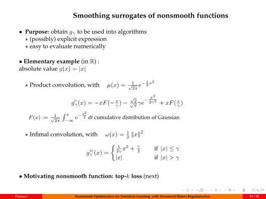
Smoothing surrogates of nonsmooth functions
• Purpose: obtain gγ to be used into algorithms? (possibly) explicit expression? easy to evaluate numerically
• Elementary example (in R) :absolute value g(x) = |x|
? Product convolution, with µ(x) = 1√2π e− 1
2x2
gcγ(x) = −xF (− xγ
)−√
2√πγe− x2
2γ2 + xF (xγ
)
F (x) := 1√2π
∫ x−∞ e−
t22 dt cumulative distribution of Gaussian
? Infimal convolution, with ω(x) = 12 ‖x‖
2
gicγ (x) = 1
2γ x2 + γ
2 if |x| ≤ γ|x| if |x| > γ
•Motivating nonsmooth function: top-k loss (next)
Pierucci Nonsmooth Optimization for Statistical Learning with Structured Matrix Regularization 11 / 33
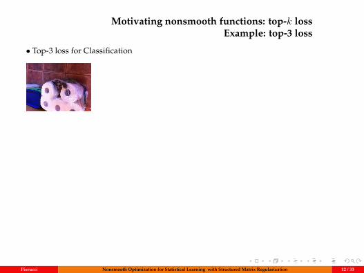
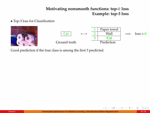
Motivating nonsmooth functions: top-k lossExample: top-3 loss
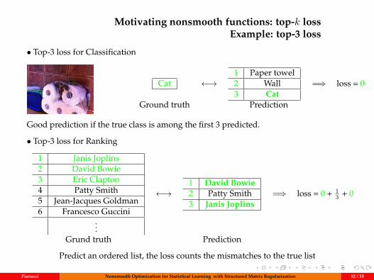
• Top-3 loss for Classification
Cat ←→1 Paper towel2 Wall3 Cat
=⇒ loss = 0
Ground truth Prediction
Good prediction if the true class is among the first 3 predicted.
• Top-3 loss for Ranking
1 Janis Joplins2 David Bowie3 Eric Clapton4 Patty Smith5 Jean-Jacques Goldman6 Francesco Guccini
...
←→1 David Bowie2 Patty Smith3 Janis Joplins
=⇒ loss = 0 + 13 + 0
Grund truth Prediction
Predict an ordered list, the loss counts the mismatches to the true list
Pierucci Nonsmooth Optimization for Statistical Learning with Structured Matrix Regularization 12 / 33
Motivating nonsmooth functions: top-k lossExample: top-3 loss
• Top-3 loss for Classification
Cat ←→1 Paper towel2 Wall3 Cat
=⇒ loss = 0
Ground truth Prediction
Good prediction if the true class is among the first 3 predicted.
• Top-3 loss for Ranking
1 Janis Joplins2 David Bowie3 Eric Clapton4 Patty Smith5 Jean-Jacques Goldman6 Francesco Guccini
...
←→1 David Bowie2 Patty Smith3 Janis Joplins
=⇒ loss = 0 + 13 + 0
Grund truth Prediction
Predict an ordered list, the loss counts the mismatches to the true list
Pierucci Nonsmooth Optimization for Statistical Learning with Structured Matrix Regularization 12 / 33
Smoothing of top-k
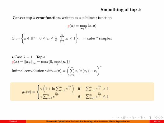
Convex top-k error function, written as a sublinear function
g(x) = maxz∈Z〈x, z〉
Z :=
z ∈ Rn : 0 ≤ zi ≤ 1k,n∑i=1
zi ≤ 1
= cube ∩ simplex
• Case k = 1 Top-1g(x) = ‖x+‖∞ = max0,max
ixi
Infimal convolution with ω(x) =(
n∑i=1
xi ln(xi)− xi)∗
gγ(x) =
γ(
1 + ln∑n
i=1 exiγ
)if
∑n
i=1 exiγ > 1
γ∑n
i=1 exiγ if
∑n
i=1 exiγ ≤ 1
xx
Pierucci Nonsmooth Optimization for Statistical Learning with Structured Matrix Regularization 13 / 33
Smoothing of top-k
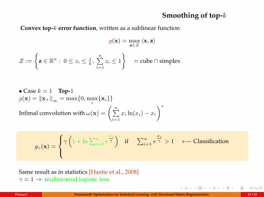
Convex top-k error function, written as a sublinear function
g(x) = maxz∈Z〈x, z〉
Z :=
z ∈ Rn : 0 ≤ zi ≤ 1k,n∑i=1
zi ≤ 1
= cube ∩ simplex
• Case k = 1 Top-1g(x) = ‖x+‖∞ = max0,max
ixi
Infimal convolution with ω(x) =(
n∑i=1
xi ln(xi)− xi)∗
gγ(x) =
γ(
1 + ln∑n
i=1 exiγ
)if
∑n
i=1 exiγ > 1 ←− Classification
Same result as in statistics [Hastie et al., 2008]γ = 1→ multinomial logistic loss
Pierucci Nonsmooth Optimization for Statistical Learning with Structured Matrix Regularization 13 / 33
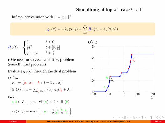
Smoothing of top-k case k > 1Infimal convolution with ω = 1
2 ‖·‖2
gγ(x) = −λ?(x, γ) +n∑i=1
Hγ(xi + λ?(x, γ))
Hγ(t) =
0 t < 012 t
2 t ∈ [0, 1k
]tk− 1
k2 t > 1k
•We need to solve an auxiliary problem(smooth dual problem)
Evaluate gγ(x) through the dual problem
DefinePx := xi, xi − k : i = 1 . . . n
Θ′(λ) = 1−∑
tj∈Pxπ[0,1/k](tj + λ)
Finda, b ∈ Px s.t. Θ′(a) ≤ 0 ≤ Θ′(b)
λ?(x, γ) = max
0, a− Θ′(a)(b−a)Θ′(b)−Θ′(a)
−20 −10 0 10 20−1
0
1
2
3∇Θ (λ)Θ′(λ)
λ
λ?b
a
tj
Pierucci Nonsmooth Optimization for Statistical Learning with Structured Matrix Regularization 14 / 33
Outline
1 Unified view of smoothing techniques
2 Conditional gradient algorithms for doubly nonsmooth learning
3 Regularization by group nuclear norm
4 Conclusion and perspectives
Pierucci Nonsmooth Optimization for Statistical Learning with Structured Matrix Regularization 15 / 33
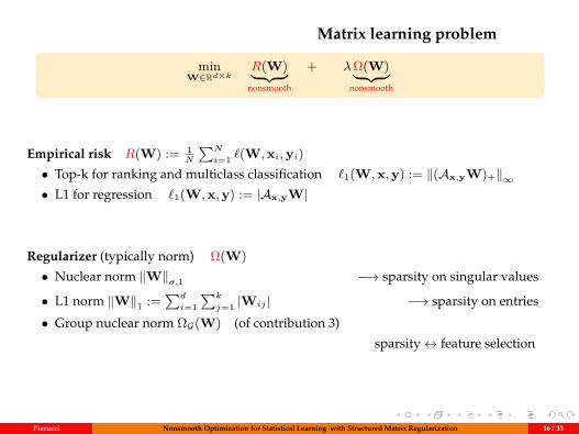
Matrix learning problem
minW∈Rd×k
R(W)︸ ︷︷ ︸nonsmooth
+ λΩ(W)︸ ︷︷ ︸nonsmooth
Empirical risk R(W) := 1N
∑N
i=1 `(W,xi,yi)• Top-k for ranking and multiclass classification `1(W,x,y) := ‖(Ax,yW)+‖∞• L1 for regression `1(W,x,y) := |Ax,yW|
Regularizer (typically norm) Ω(W)• Nuclear norm ‖W‖σ,1 −→ sparsity on singular values
• L1 norm ‖W‖1 :=∑d
i=1
∑k
j=1 |Wij | −→ sparsity on entries
• Group nuclear norm ΩG(W) (of contribution 3)
sparsity↔ feature selection
Pierucci Nonsmooth Optimization for Statistical Learning with Structured Matrix Regularization 16 / 33

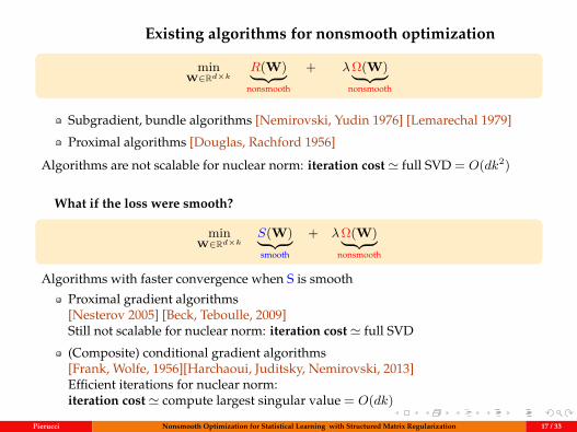
Existing algorithms for nonsmooth optimization
minW∈Rd×k
R(W)︸ ︷︷ ︸nonsmooth
+ λΩ(W)︸ ︷︷ ︸nonsmooth
Subgradient, bundle algorithms [Nemirovski, Yudin 1976] [Lemarechal 1979]
Proximal algorithms [Douglas, Rachford 1956]
Algorithms are not scalable for nuclear norm: iteration cost ' full SVD = O(dk2)
What if the loss were smooth?
minW∈Rd×k
S(W)︸ ︷︷ ︸smooth
+ λΩ(W)︸ ︷︷ ︸nonsmooth
Algorithms with faster convergence when S is smooth
Proximal gradient algorithms[Nesterov 2005] [Beck, Teboulle, 2009]Still not scalable for nuclear norm: iteration cost ' full SVD
(Composite) conditional gradient algorithms[Frank, Wolfe, 1956][Harchaoui, Juditsky, Nemirovski, 2013]Efficient iterations for nuclear norm:iteration cost ' compute largest singular value = O(dk)
Pierucci Nonsmooth Optimization for Statistical Learning with Structured Matrix Regularization 17 / 33
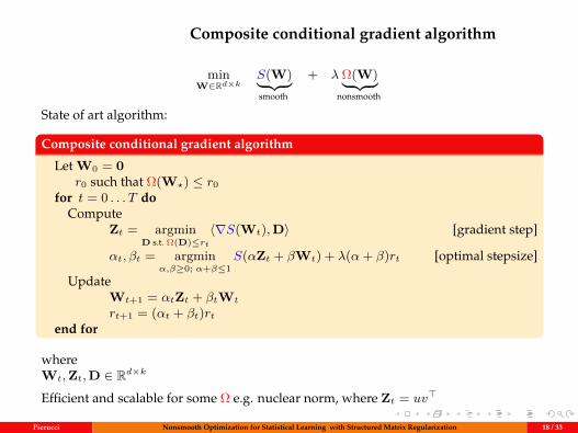
Composite conditional gradient algorithm
minW∈Rd×k
S(W)︸ ︷︷ ︸smooth
+ λ Ω(W)︸ ︷︷ ︸nonsmooth
State of art algorithm:
Composite conditional gradient algorithm
Let W0 = 0r0 such that Ω(W?) ≤ r0
for t = 0 . . . T doCompute
Zt = argminD s.t. Ω(D)≤rt
〈∇S(Wt),D〉 [gradient step]
αt, βt = argminα,β≥0; α+β≤1
S(αZt + βWt) + λ(α+ β)rt [optimal stepsize]
UpdateWt+1 = αtZt + βtWt
rt+1 = (αt + βt)rtend for
whereWt,Zt,D ∈ Rd×k
Efficient and scalable for some Ω e.g. nuclear norm, where Zt = uv>
Pierucci Nonsmooth Optimization for Statistical Learning with Structured Matrix Regularization 18 / 33
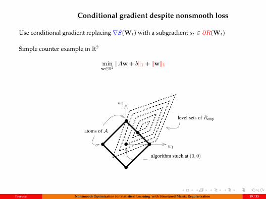
Conditional gradient despite nonsmooth loss
Use conditional gradient replacing∇S(Wt) with a subgradient st ∈ ∂R(Wt)
Simple counter example in R2
minw∈R2
‖Aw + b‖1 + ‖w‖1
4 Federico Pierucci et al.
Algorithm 1 Composite Conditional GradientInputs: , Initialize W0 = 0, t = 1for k = 0 . . . K do
Call the linear minimization oracle: LMO(Wk)Compute
min1,...,t0
tX
i=1
i + R
tX
i=1
iai
!
Increment t t + 1end forReturn W =
Pi iai
Algorithm 2 Conditional gradient algorithm: Frank-WolfeInputInitialize W0 = 0, t = 1for k = 0 . . . K do
Call linear minimization oracle adaptiveak LMO(Wt)Set step-size ↵k = 2/(2 + k)Update Wk+1 (1 ↵k)Wk + ↵kak
end forReturn WK
2.3 How about nonsmooth empirical risk?
Composite conditional gradient assumes that the empirical risk in the objective function g is smooth.Indeed, at each iteration, the algorithm requires to computerR(W ). Should we consider nonsmooth lossfunctions, such as the `1-loss or the hinge-loss, the convergence of the algorithm is unclear if we replacethe gradient by a subgradient in @R(W ). In fact, we can produce a simple counterexample showing thatthe corresponding algorithm can get stuck in a suboptimal point.
Let us describe and draw in Figure 1 a counterexample in two dimensions (generalization to higher di-mension is straightforward). We consider the `1-norm with its four atoms (1, 0), (0, 1), (1, 0), (0,1)and a convex function of the type of a translated weighted `1-norm
f(w1, w2) = |w1 + w2 3/2| + 4 |w2 w1| .
level sets of Remp
w1
w2
atoms of A
algorithm stuck at (0, 0)
Fig. 1 Drawing of a situation where the algorithm using a subgradient of a nonsmooth empirical risk does not converge.
We observe that the four directions given by the atoms go from (0, 0) towards level-sets of R withlarger values. This yields that, for small , the minimization of the objective function on these directions
Pierucci Nonsmooth Optimization for Statistical Learning with Structured Matrix Regularization 19 / 33
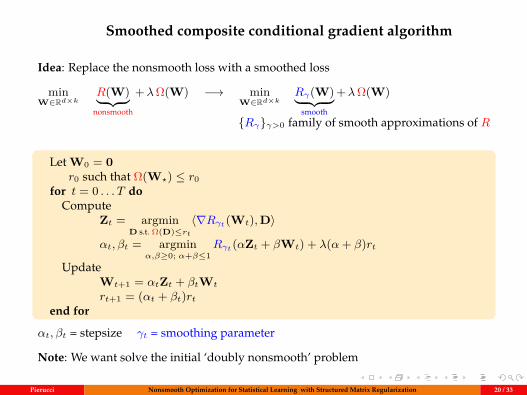
Smoothed composite conditional gradient algorithm
Idea: Replace the nonsmooth loss with a smoothed loss
minW∈Rd×k
R(W)︸ ︷︷ ︸nonsmooth
+λΩ(W) −→ minW∈Rd×k
Rγ(W)︸ ︷︷ ︸smooth
+λΩ(W)
Rγγ>0 family of smooth approximations of R
Let W0 = 0r0 such that Ω(W?) ≤ r0
for t = 0 . . . T doCompute
Zt = argminD s.t. Ω(D)≤rt
〈∇Rγt (Wt),D〉
αt, βt = argminα,β≥0; α+β≤1
Rγt (αZt + βWt) + λ(α+ β)rt
UpdateWt+1 = αtZt + βtWt
rt+1 = (αt + βt)rtend for
αt, βt = stepsize γt = smoothing parameter
Note: We want solve the initial ‘doubly nonsmooth’ problem
Pierucci Nonsmooth Optimization for Statistical Learning with Structured Matrix Regularization 20 / 33
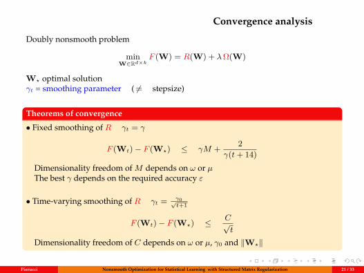
Convergence analysis
Doubly nonsmooth problem
minW∈Rd×k
F (W) = R(W) + λΩ(W)
W? optimal solutionγt = smoothing parameter ( 6= stepsize)
Theorems of convergence
• Fixed smoothing of R γt = γ
F (Wt)− F (W?) ≤ γM + 2γ(t+ 14)
Dimensionality freedom of M depends on ω or µThe best γ depends on the required accuracy ε
• Time-varying smoothing of R γt = γ0√t+1
F (Wt)− F (W?) ≤ C√t
Dimensionality freedom of C depends on ω or µ, γ0 and ‖W?‖
Pierucci Nonsmooth Optimization for Statistical Learning with Structured Matrix Regularization 21 / 33
Algoritm implementation
PackageAll the Matlab code written from scratch, in particular:
• Multiclass SVM
• Top-k multiclass SVM
• All other smoothed functions
MemoryEfficient memory management
• Tools to operate with low rank variables
• Tools to work with sparse sub-matrices of low rank matrices (collaborative filtering)
Numerical experiments - 2 motivating applications
• Fix smoothing - matrix completion (regression)
• Time-varying smoothing - top-5 multiclass classification
Pierucci Nonsmooth Optimization for Statistical Learning with Structured Matrix Regularization 22 / 33
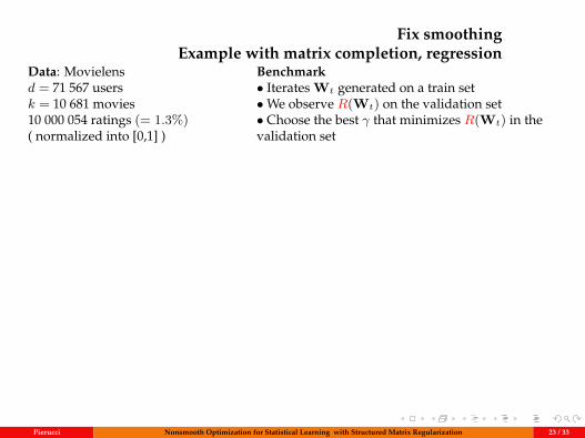
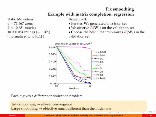
Fix smoothingExample with matrix completion, regression
Data: Movielensd = 71 567 usersk = 10 681 movies10 000 054 ratings (= 1.3%)( normalized into [0,1] )
Benchmark• Iterates Wt generated on a train set•We observe R(Wt) on the validation set• Choose the best γ that minimizes R(Wt) in thevalidation set
100
1020.188
0.2457
0.3211
0.4196
0.5484
0.7167
iterations
Emp. risk on validation set, λ=10−6
γ = 0.001γ = 0.01γ = 0.1γ = 0.5γ = 1γ = 5γ = 10γ = 50γ = best
Each γ gives a different optimization problem
Tiny smoothing→ slower convergenceLarge smoothing→ objective much different than the initial one
Pierucci Nonsmooth Optimization for Statistical Learning with Structured Matrix Regularization 23 / 33
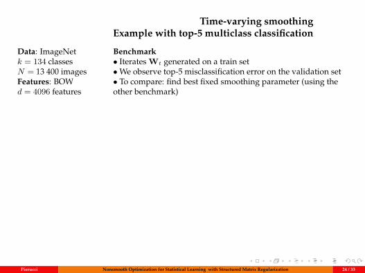
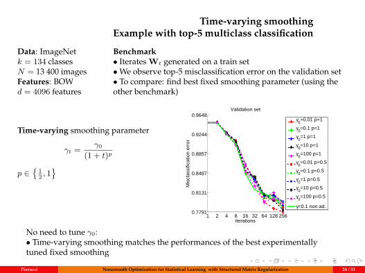
Time-varying smoothingExample with top-5 multiclass classification
Data: ImageNetk = 134 classesN = 13 400 imagesFeatures: BOWd = 4096 features
Benchmark• Iterates Wt generated on a train set•We observe top-5 misclassification error on the validation set• To compare: find best fixed smoothing parameter (using theother benchmark)
Time-varying smoothing parameter
γt = γ0
(1 + t)p
p ∈
12 , 1
1 2 4 8 16 32 64 128 2560.7791
0.8131
0.8487
0.8857
0.9244
0.9648Validation set
iterations
Mis
clas
sific
atio
n er
ror
γ0=0.01 p=1
γ0=0.1 p=1
γ0=1 p=1
γ0=10 p=1
γ0=100 p=1
γ0=0.01 p=0.5
γ0=0.1 p=0.5
γ0=1 p=0.5
γ0=10 p=0.5
γ0=100 p=0.5
γ=0.1 non ad.
No need to tune γ0:• Time-varying smoothing matches the performances of the best experimentallytuned fixed smoothing
Pierucci Nonsmooth Optimization for Statistical Learning with Structured Matrix Regularization 24 / 33
Outline
1 Unified view of smoothing techniques
2 Conditional gradient algorithms for doubly nonsmooth learning
3 Regularization by group nuclear norm
4 Conclusion and perspectives
Pierucci Nonsmooth Optimization for Statistical Learning with Structured Matrix Regularization 25 / 33
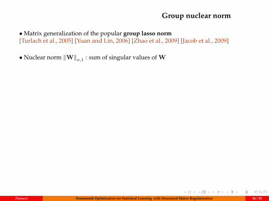
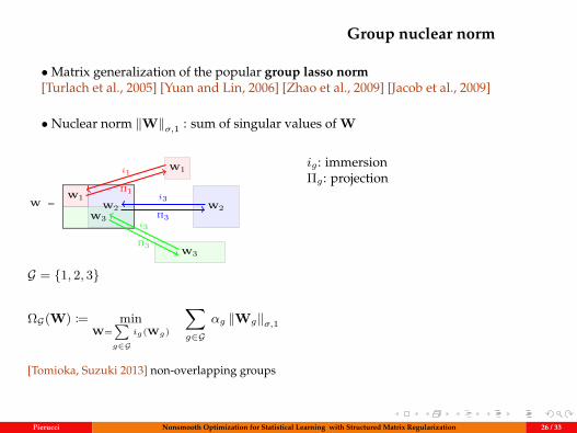
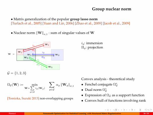
Group nuclear norm
•Matrix generalization of the popular group lasso norm[Turlach et al., 2005] [Yuan and Lin, 2006] [Zhao et al., 2009] [Jacob et al., 2009]
• Nuclear norm ‖W‖σ,1 : sum of singular values of W
W1
W2
W3
W2W3
W1W =
i1
Π1
i3
Π3
i3
Π3
G = 1, 2, 3
ΩG(W) := minW=∑g∈G
ig(Wg)
∑g∈G
αg ‖Wg‖σ,1
[Tomioka, Suzuki 2013] non-overlapping groups
ig : immersionΠg : projection
Convex analysis - theoretical study
• Fenchel conjugate Ω∗G• Dual norm ΩG• Expression of ΩG as a support function
• Convex hull of functions involving rank
Pierucci Nonsmooth Optimization for Statistical Learning with Structured Matrix Regularization 26 / 33
Convex hull - Results
In words, the convex hull is the largest convex function lying below the given one
Properly restricted to a ball,the nuclear norm is the convex hull of rank [Fazel 2001]→ generalization
Theorem
Properly restricted to a ball, group nuclear norm is the convex hull of:
• The ‘reweighted group rank’ function:
ΩrankG (W) := inf
W=∑g∈G
ig(Wg)
∑g∈G
αg rank(Wg)
• The ‘reweighted restricted rank’ function:
Ωrank(W) := ming∈G
αg rank(W) + δg(W)
δg indicator function
Learning with group nuclear norm enforces low-rank property on groups
Pierucci Nonsmooth Optimization for Statistical Learning with Structured Matrix Regularization 27 / 33

Learning with group nuclear norm
Usual optimization algorithms can handle the group nuclear norm:? composite conditional gradient algorithms? (accelerated) proximal gradient algorithms
Illustration with proximal gradient optimization algorithmThe key computations are parallelized on each group
Good scalability when there are many small groups
• prox of group nuclear norm
proxγΩG ((Wg)g) =(UgDγ(Sg)Vg
>)g∈G
where Dγ : soft thresholding operator
• SVD decompositionWg = UgSgVg
>
Dγ(S) = Diag(maxsi − γ, 01≤i≤r).
Package in Matlab, in particular:→ vector space of group nuclear norm, overloading of + *
Pierucci Nonsmooth Optimization for Statistical Learning with Structured Matrix Regularization 28 / 33
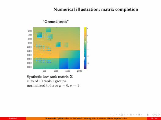
Numerical illustration: matrix completion
“Ground truth”data
500 1000 1500 2000
200
400
600
800
1000
1200
1400
1600
1800
2000
-3
-2
-1
0
1
2
Synthetic low rank matrix Xsum of 10 rank-1 groupsnormalized to have µ = 0, σ = 1
Pierucci Nonsmooth Optimization for Statistical Learning with Structured Matrix Regularization 29 / 33
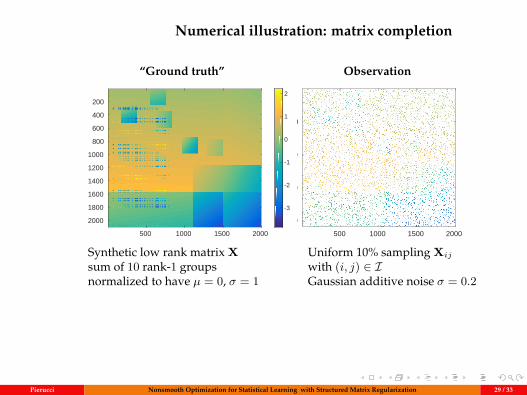
Numerical illustration: matrix completion
“Ground truth” Observationdata
500 1000 1500 2000
200
400
600
800
1000
1200
1400
1600
1800
2000
-3
-2
-1
0
1
2
observations
500 1000 1500 2000
500
1000
1500
2000
-3
-2
-1
0
1
2
Synthetic low rank matrix Xsum of 10 rank-1 groupsnormalized to have µ = 0, σ = 1
Uniform 10% sampling Xij
with (i, j) ∈ IGaussian additive noise σ = 0.2
Pierucci Nonsmooth Optimization for Statistical Learning with Structured Matrix Regularization 29 / 33
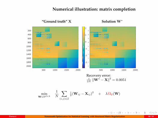
Numerical illustration: matrix completion
“Ground truth” X Solution W?
data
500 1000 1500 2000
200
400
600
800
1000
1200
1400
1600
1800
2000
-3
-2
-1
0
1
2
solution
500 1000 1500 2000
200
400
600
800
1000
1200
1400
1600
1800
2000
-3
-2
-1
0
1
2
Recovery error:1
2N ‖W? −X‖2 = 0.0051
minW∈Rd×k
1N
∑(i,j)∈I
12 (Wij −Xij)2 + λΩG(W)
Pierucci Nonsmooth Optimization for Statistical Learning with Structured Matrix Regularization 30 / 33
Outline
1 Unified view of smoothing techniques
2 Conditional gradient algorithms for doubly nonsmooth learning
3 Regularization by group nuclear norm
4 Conclusion and perspectives
Pierucci Nonsmooth Optimization for Statistical Learning with Structured Matrix Regularization 31 / 33
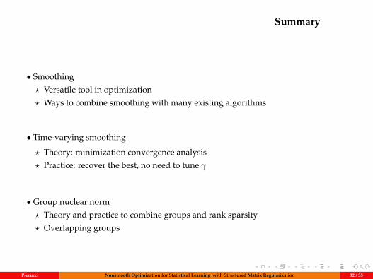
Summary
• Smoothing
? Versatile tool in optimization
? Ways to combine smoothing with many existing algorithms
• Time-varying smoothing
? Theory: minimization convergence analysis
? Practice: recover the best, no need to tune γ
• Group nuclear norm
? Theory and practice to combine groups and rank sparsity
? Overlapping groups
Pierucci Nonsmooth Optimization for Statistical Learning with Structured Matrix Regularization 32 / 33
Perspectives
• Smoothing for faster convergence:Moreau-Yosida smoothing can be used to improve the condition number of poorlyconditioned objectives before applying linearly-convergent convex optimizationalgorithms [Hongzhou et al. 2017]
• Smoothing for better prediction:Smoothing can be adapted to properties of the dataset and be used to improve theprediction performance of machine learning algorithms
• Learning group structure and weights for better prediction:The group structure in the group nuclear norm can be learned to leveragedunderlying structure and improve the prediction
• Extensions to group Schatten norm
• Potential applications of group nuclear norm
? multi-attribute classification
? multiple tree hierarchies
? dimensionality reduction, feature selection e.g. concatenate features, avoid PCA
Thank You
Pierucci Nonsmooth Optimization for Statistical Learning with Structured Matrix Regularization 33 / 33