10/21/15
1
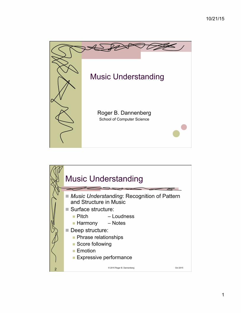
Music Understanding
Roger B. Dannenberg School of Computer Science
2
Music Understanding
Music Understanding: Recognition of Pattern and Structure in Music
Surface structure: Pitch – Loudness Harmony – Notes
Deep structure: Phrase relationships Score following Emotion Expressive performance
© 2015 Roger B. Dannenberg Oct 2015
10/21/15
2
3
Accompaniment Video
© 2015 Roger B. Dannenberg Oct 2015 Oct 2015
4
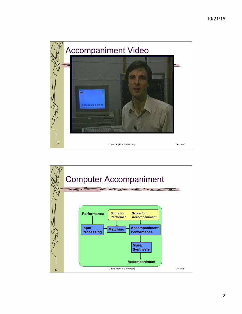
Computer Accompaniment
Performance
Input Processing
Matching
Score for Performer
Score for Accompaniment
Accompaniment Performance
Music Synthesis
Accompaniment
© 2015 Roger B. Dannenberg Oct 2015
10/21/15
3
5
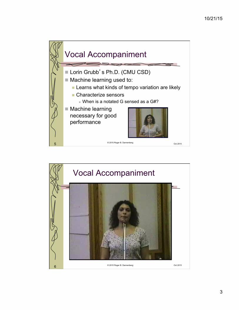
Vocal Accompaniment
Lorin Grubb’s Ph.D. (CMU CSD) Machine learning used to:
Learns what kinds of tempo variation are likely Characterize sensors
When is a notated G sensed as a G#?
Machine learning necessary for good performance
© 2015 Roger B. Dannenberg Oct 2015
6
Vocal Accompaniment
© 2015 Roger B. Dannenberg Oct 2015
10/21/15
4
7
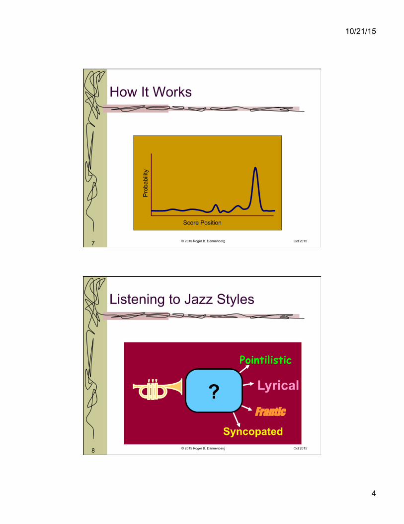
How It Works
Pro
babi
lity
Score Position
© 2015 Roger B. Dannenberg Oct 2015
8
Listening to Jazz Styles
? Lyrical
Pointilistic
Syncopated
Frantic
© 2015 Roger B. Dannenberg Oct 2015
10/21/15
5
9
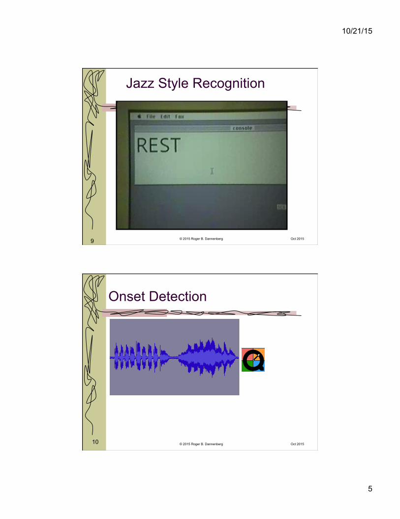
Jazz Style Recognition
© 2015 Roger B. Dannenberg Oct 2015
10
Onset Detection
© 2015 Roger B. Dannenberg Oct 2015
10/21/15
6
11
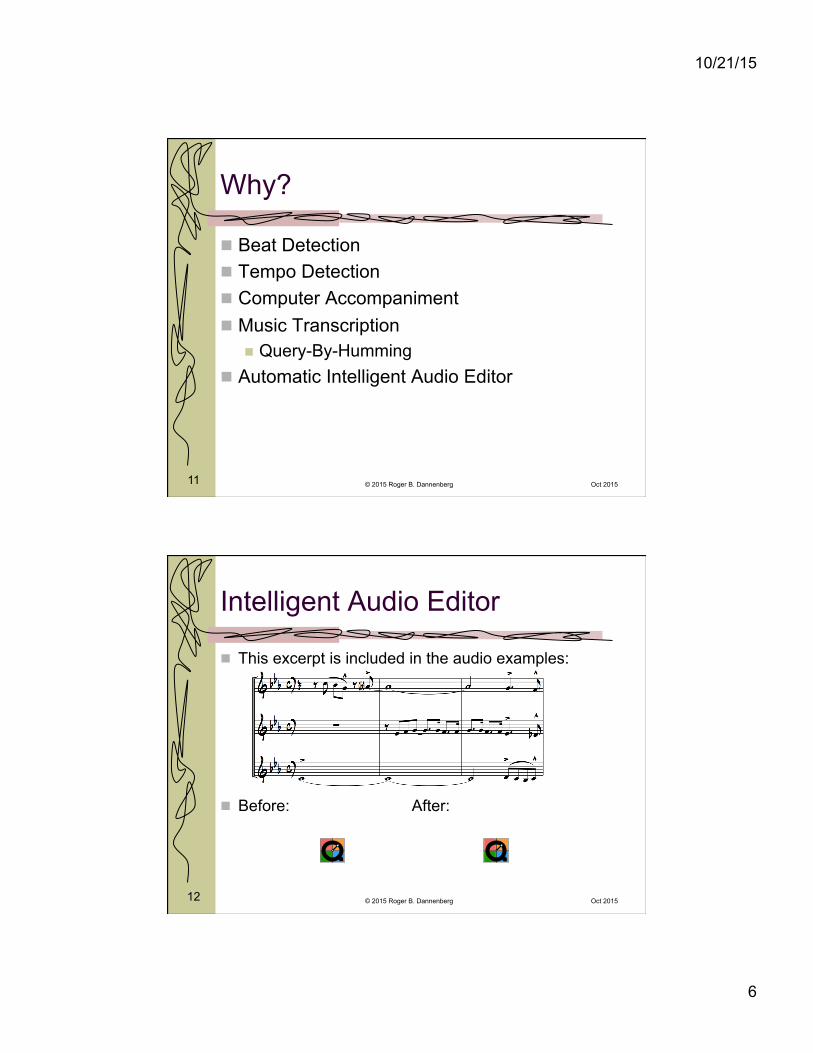
Why?
Beat Detection Tempo Detection Computer Accompaniment Music Transcription
Query-By-Humming Automatic Intelligent Audio Editor
© 2015 Roger B. Dannenberg Oct 2015
12
Intelligent Audio Editor
This excerpt is included in the audio examples:
Before: After:
© 2015 Roger B. Dannenberg Oct 2015
10/21/15
7
13
Some Approaches
Features and Thresholds High Frequency Phase Change
Neural Networks Hierarchical Models HMM
© 2015 Roger B. Dannenberg Oct 2015
A Bootstrap Method for Training an Accurate Audio Segmenter
Ning Hu and Roger B. Dannenberg Carnegie Mellon University
10/21/15
8
15
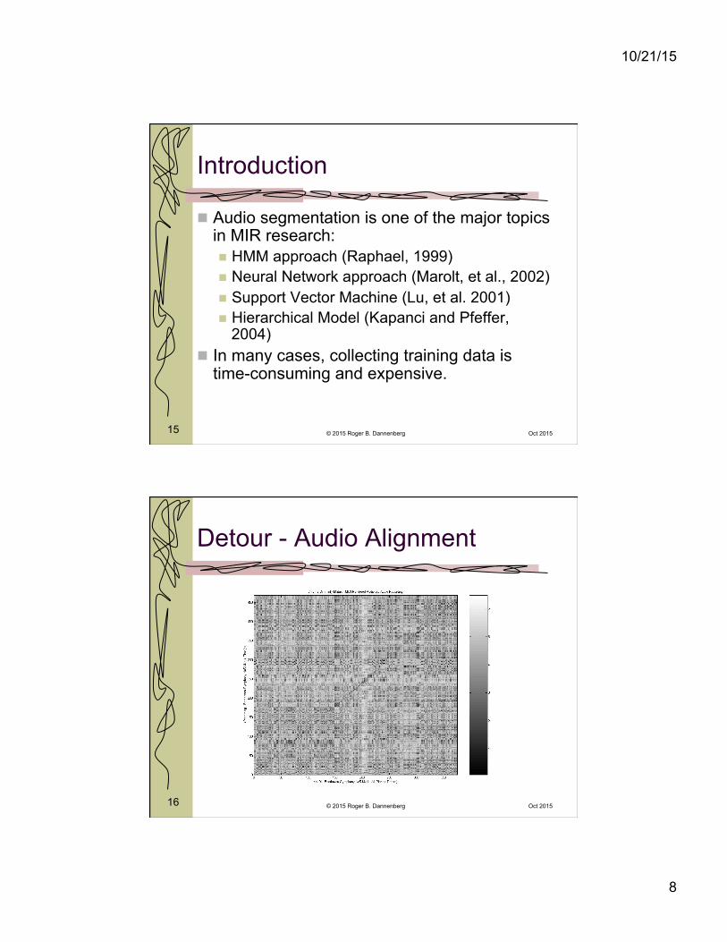
Introduction
Audio segmentation is one of the major topics in MIR research: HMM approach (Raphael, 1999) Neural Network approach (Marolt, et al., 2002) Support Vector Machine (Lu, et al. 2001) Hierarchical Model (Kapanci and Pfeffer,
2004) In many cases, collecting training data is
time-consuming and expensive.
© 2015 Roger B. Dannenberg Oct 2015
16
Detour - Audio Alignment
© 2015 Roger B. Dannenberg Oct 2015
10/21/15
9
17
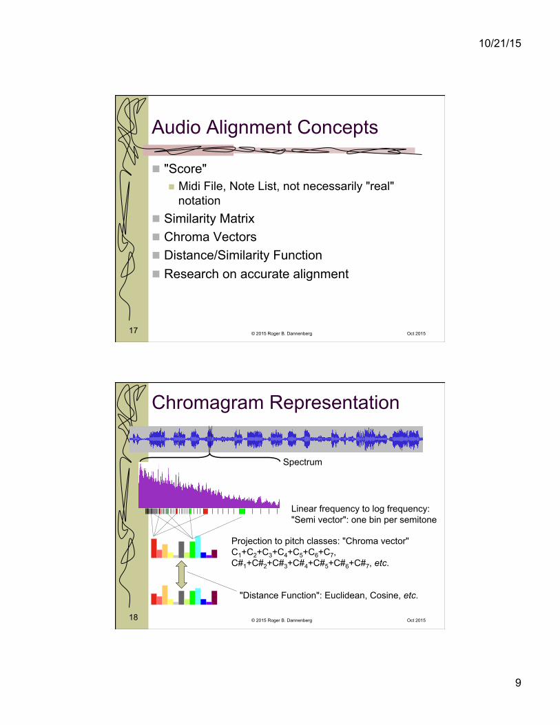
Audio Alignment Concepts
"Score" Midi File, Note List, not necessarily "real"
notation Similarity Matrix Chroma Vectors Distance/Similarity Function Research on accurate alignment
© 2015 Roger B. Dannenberg Oct 2015
Chromagram Representation
Spectrum
Linear frequency to log frequency: "Semi vector": one bin per semitone
Projection to pitch classes: "Chroma vector" C1+C2+C3+C4+C5+C6+C7, C#1+C#2+C#3+C#4+C#5+C#6+C#7, etc.
"Distance Function": Euclidean, Cosine, etc.
Oct 2015 © 2015 Roger B. Dannenberg 18
10/21/15
10
19
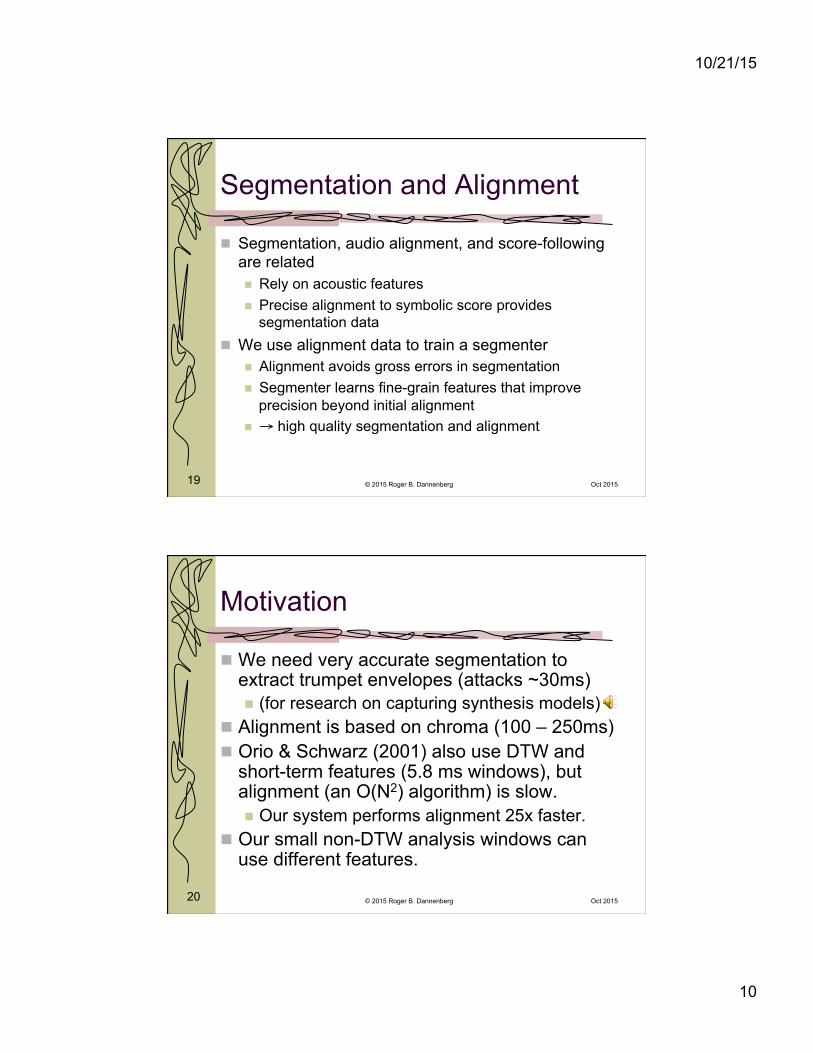
Segmentation and Alignment
Segmentation, audio alignment, and score-following are related Rely on acoustic features Precise alignment to symbolic score provides
segmentation data We use alignment data to train a segmenter
Alignment avoids gross errors in segmentation Segmenter learns fine-grain features that improve
precision beyond initial alignment → high quality segmentation and alignment
© 2015 Roger B. Dannenberg Oct 2015
20
Motivation
We need very accurate segmentation to extract trumpet envelopes (attacks ~30ms) (for research on capturing synthesis models)
Alignment is based on chroma (100 – 250ms) Orio & Schwarz (2001) also use DTW and
short-term features (5.8 ms windows), but alignment (an O(N2) algorithm) is slow. Our system performs alignment 25x faster.
Our small non-DTW analysis windows can use different features.
© 2015 Roger B. Dannenberg Oct 2015
10/21/15
11
21
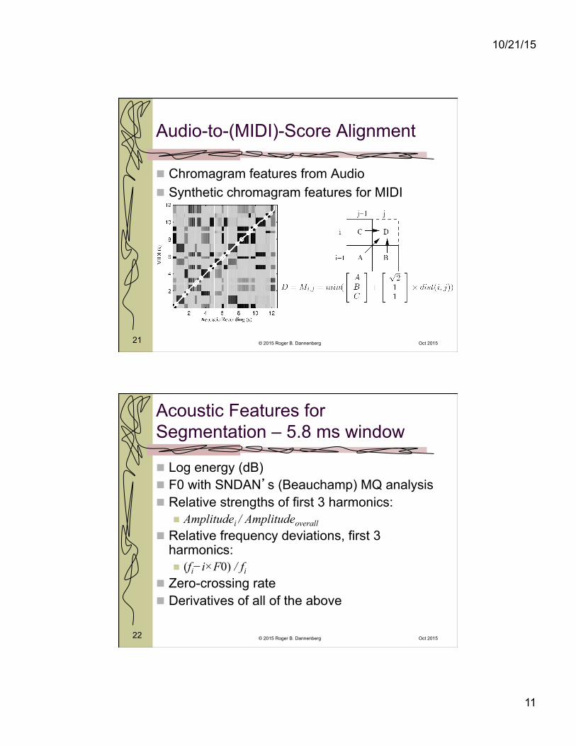
Audio-to-(MIDI)-Score Alignment
Chromagram features from Audio Synthetic chromagram features for MIDI
© 2015 Roger B. Dannenberg Oct 2015
22
Acoustic Features for Segmentation – 5.8 ms window
Log energy (dB) F0 with SNDAN’s (Beauchamp) MQ analysis Relative strengths of first 3 harmonics:
Amplitudei / Amplitudeoverall Relative frequency deviations, first 3
harmonics: (fi−i×F0) / fi
Zero-crossing rate Derivatives of all of the above
© 2015 Roger B. Dannenberg Oct 2015
10/21/15
12
23
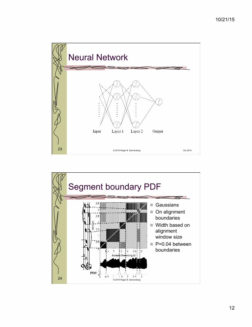
Neural Network
© 2015 Roger B. Dannenberg Oct 2015
24
Segment boundary PDF
Gaussians On alignment
boundaries Width based on
alignment window size
P=0.04 between boundaries
© 2015 Roger B. Dannenberg
10/21/15
13
25
Bootstrap learning process
Multiply neural net output by PDF For each neighborhood around a segment
boundary, find the peak → “adjusted onset” Retrain the neural network:
adjusted onsets are 1, other points are 0
© 2015 Roger B. Dannenberg Oct 2015
26
Results
Model
Baseline Segmenter
Segmenter w/ Bootstrap
Miss Rate
8.8%
0.0%
Spurious Rate
10.3%
0.3%
Av. Error
21 ms
10 ms
STD
29 ms
14 ms
Model
Baseline Segmenter
Segmenter w/ Bootstrap
Miss Rate
15.0%
2.0%
Spurious Rate
25.0%
4.0%
Av. Error
35 ms
8 ms
STD
48 ms
12 ms
SYN
THET
IC
REA
L
© 2015 Roger B. Dannenberg Oct 2015
10/21/15
14
27
Sound Examples
Input
Output – segmenter was trained on similar data using the bootstrap method. This input was segmented without using any score information.
© 2015 Roger B. Dannenberg Oct 2015
© 2015 Roger B. Dannenberg 28
Conclusions
Supervised learning often wins over hand-crafted systems
Segmentation training data is expensive, so supervised training is difficult
Alignment provides strong hints, but not accurate enough for training
Bootstrapping allows segmenter to generate its own training data
Dramatic improvements in accuracy, even when tested without alignment “hints”
Oct 2015
10/21/15
15
Summary
Computer Accompaniment Offline Score Alignment Onset Detection
© 2015 Roger B. Dannenberg 29 Oct 2015
Recommended