Machine Learning for Optical

Modulation Format Recognition

Ricard Boada Farràs

Bachelor Thesis

S136096

May 2014

DTU Fotonik, Technical University of Denmark, Kgs. Lyngby, Denmark

Supervised by:

Idelfonso Tafur Monroy

Robert Borkowski

2

3

Machine Learning for Optical

Modulation Format Recognition

Ricard Boada Farràs

Bachelor Thesis

S136096

May 2014

DTU Fotonik, Technical University of Denmark, Kgs. Lyngby, Denmark

Supervised by:

Idelfonso Tafur Monroy

Robert Borkowski

4

Name of the thesis

Machine Learning for Optical Modulation Format Recognition

Author(s):

Ricard Boada Farràs

Supervisor(s):

Idelfonso Tafur Monroy (DTU Fotonik)

Robert Borkowski (DTU Fotonik)

This report is a part of the requirements to achieve the Bachelor of Science (BSc) in Telecommunications at Technical University of Denmark.

The report represents 15 ECTS points.

Department of Photonics Engineering

Technical University of Denmark

Oersted Plads, Building 343

DK-2800 Kgs. Lyngby

Denmark

www.fotonik.dtu.dk

Tel: (+45) 45 25 63 52

Fax: (+45) 45 93 65 81

E-mail: info@fotonik.dtu.dk

5

Abstract

Next generation of optical networks will necessitate the use of advanced

functionalities in the transceivers. In particular, modulation format recognition will

enable dynamically switched energy efficient networks that can adapt to traffic demand

and optimize resource utilization.

This thesis presents the first comparison of clustering algorithms applied to

modulation format recognition in Stokes space. 2-, 4-, 8-PSK and 8-, 12-, 16-QAM

modulation formats are recognized and the requirements in terms of OSNR

performance, accuracy and complexity are analyzed.

A novel technique is also proposed for modulation format recognition in Stokes

space, based on maximum likelihood between the received signal and the characteristics

of the modulations targeted, showing OSNR requirements lower than those in the

previously published literature.

6

7

Acknowledgements

First of all, I would like to express my gratitude to Professor Idelfonso Tafur

Monroy for giving me the opportunity to join the Metro-Access & Short Range

Communications Group at DTU Fotonik and helping me with my stay in Denmark.

Thanks to him and also to my co-supervisor, PhD Robert Borkowski, for all their

support during the thesis. I feel highly indebt for all the feedback and advice they gave

me on my daily work.

I would also like to acknowledge Joan M. Gené Bernaus, from Polytechnic

University of Catalonia, for encouraging me to do my thesis in DTU and helping me

before and during the whole project.

I wish to thank my department colleagues and especially my office workmates,

Los Boludos del 358, for all the good moments since I arrived in Denmark. Further

thanks to my classmates, Els Competitius, from Barcelona, who have always been there

during these four years.

Finally, none of this would have been possible without the patience and belief of

my parents, my sister, my family and my friends. Thank you so much.

8

9

Table of Contents

Abstract ............................................................................................................................. 5

Acknowledgements .......................................................................................................... 7

Table of Contents ............................................................................................................. 9

Acronyms ....................................................................................................................... 11

List of Figures ................................................................................................................. 12

List of Tables .................................................................................................................. 14

1 Introduction .................................................................................................. 15

1.1 Motivation ............................................................................................. 15

1.2 Problem statement ................................................................................. 17

1.3 State of the Art ...................................................................................... 18

1.4 Methodology ......................................................................................... 20

1.5 Contributions ........................................................................................ 21

1.6 Thesis outline ........................................................................................ 21

2 Polarization demultiplexing ......................................................................... 23

2.1 Polarization demultiplexing in Stokes space ........................................ 24

2.2 Representation of Stokes parameters in the Poincaré sphere ................ 26

3 Machine Learning ........................................................................................ 29

3.1 Clustering algorithms ............................................................................ 30

3.1.1 K-Means ............................................................................................ 31

3.1.2 Expectation Maximization (EM) ....................................................... 33

3.1.3 Density Based Spatial Clustering of Application with Noise

(DBSCAN) ………………………………………………………………………36

3.1.4 Ordering Points to Identify the Clustering Structure (OPTICS) ....... 39

3.1.5 Spectral Clustering ............................................................................ 41

3.1.6 Gravitational Clustering .................................................................... 43

10

3.1.7 Clustering algorithms comparison .................................................... 46

3.2 Clustering evaluation techniques .......................................................... 47

4 Proposed algorithm for modulation format recognition based on Maximum

Likelihood in Stokes space ............................................................................................. 51

4.1 Proposed algorithm ............................................................................... 51

4.2 Conclusions ........................................................................................... 54

5 Simulation .................................................................................................... 55

5.1 Simulation setup ................................................................................... 55

5.2 FEC limit ............................................................................................... 56

5.3 Simulation results ................................................................................. 57

6 Conclusions .................................................................................................. 61

6.1 Future work ........................................................................................... 62

7 References .................................................................................................... 63

11

Acronyms

AMI Adjusted Mutual Information

ANN Artificial Neural Networks

CD Chromatic Dispersion

CDist Core Distance

CMA Constant Modulus Algorithm

CON Cognitive Optical Network

DBSCAN Density-Based Spatial Clustering of Application with Noise

DGD Differential Group Delay

DSP Digital Signal Processor

EM Expectation Maximization

FEC Forward Error Correction

GMM Gaussian Mixture Model

HOS High-Order Statistics

I/Q In-phase/Quadrature

MFR Modulation Format Recognition

ML Maximum Likelihood

OBS Optical Burst Switching

OCR Optical Character Recognition

OOK On-off Keying

OPTICS Ordering Points to Identify Clustering Structure

OSNR Optical Signal to Noise Ratio

PBS Polarization Beam Splitter

PDL Polarization Dependent Losses

PDM Polarization Division Multiplexing

PMD Polarization Mode Dispersion

PSK Phase-Shift Keying

QAM Quadrature Amplitude Modulation

QoS Quality of Service

RDist Reachability Distance

SAE Software Adaptable Element

SOP State Of Polarization

WDM Wavelength Division Multiplexing

12

List of Figures

Figure 1.1. Global IP traffic evolution between 2012 and 2017 [1]. ............................. 15

Figure 1.2. Interaction between different elements in a cognitive network. ................. 17

Figure 1.3. Example of two modulation formats and their corresponding Poincaré

sphere. ............................................................................................................................. 18

Figure 1.4. Coherent receivers’ DSP flows of state-of-the-art techniques on optical

modulation format recognition. ...................................................................................... 20

Figure 2.1. Orthogonal polarization states ..................................................................... 23

Figure 2.2. Different PDM formats constellations (top) with their corresponding Stokes

space representation in the Poincaré sphere ................................................................... 26

Figure 2.3. Illustration of the Poincaré sphere. .............................................................. 27

Figure 3.1. Illustration of the clustering process ........................................................... 30

Figure 3.2. Example of K-Means performance on a 2D space with two clusters. ........ 32

Figure 3.3. K-Means flow chart. .................................................................................... 33

Figure 3.4. Example of Expectation Maximization applied with a Gaussian Mixture

Model formed by two clusters ........................................................................................ 34

Figure 3.5. EM flow chart.............................................................................................. 36

Figure 3.6. Definitions necessary for density-based algorithms with respect to

MinPts=3. ....................................................................................................................... 37

Figure 3.7. Data set recognizable using a density-based method, non-detectable by

other techniques like K-Means. ...................................................................................... 37

Figure 3.8. Flow chart of DBSCAN. ............................................................................. 38

Figure 3.9. Core distance and reachability distances with MinPts=4. ........................... 39

Figure 3.10. OPTICS flow chart. ................................................................................... 40

Figure 3.11. Spectral clustering dimensionality reduction. Comparison before (a) and

after (b) spectral technique, for 25 dB PDM BPSK signal. ............................................ 41

Figure 3.12. Spectral methods flow chart. ..................................................................... 43

13

Figure 3.13. Gravitational clustering evolution over time. ............................................ 44

Figure 3.14. Flow chart of Gravitational Clustering...................................................... 45

Figure 3.15. Difference between a(i) and b(i) in the computation of Silhouette

coefficient. ...................................................................................................................... 47

Figure 3.16. Modulation format recognition using Silhouette coefficient. ................... 48

Figure 4.1. Rotation suffered in the Poincaré sphere around S1. ................................... 51

Figure 4.2. QPSK initial centroids' positions used as a reference to obtain the optimum

angle. .............................................................................................................................. 52

Figure 4.3. Poincaré sphere for a 20 dB QPSK signal with π/16 radians rotation. ....... 53

Figure 4.4. Proposed algorithm flow chart. ................................................................... 54

Figure 5.1. FEC limit in terms of the minimum required OSNR for different

modulations, computed with 28Gbaud at 0.1nm linewidth. ........................................... 57

Figure 5.2. OSNR performance of the algorithms for different modulation formats. ... 58

Figure 5.3. Reliability of different clustering algorithms according to AMI index. ..... 60

Figure 5.4. Complexity of clustering algorithms measured in terms of clustering time

spent. ............................................................................................................................... 60

Figure 6.1. Real configuration of optical network with 2 transmitters and a single

receiver. .......................................................................................................................... 62

14

List of Tables

Table 3.1. Comparison of different clustering algorithms analyzed. ............................. 46

Table 5.1. Categories to be simulated for each modulation format. .............................. 55

Table 5.2. Parameters selection for the simulation test. ................................................ 56

Table 5.3. FEC threshold for different modulation formats .......................................... 56

15

1 Introduction

1.1 Motivation

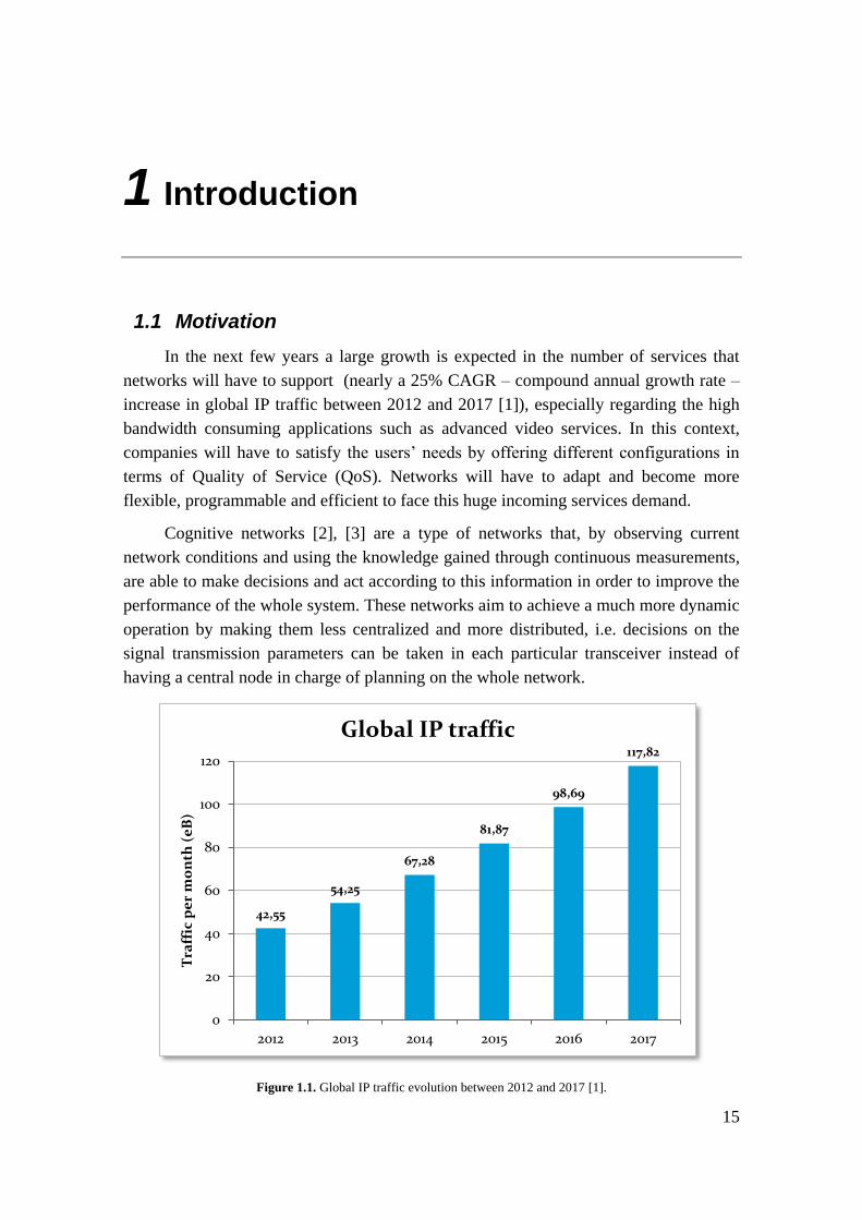
In the next few years a large growth is expected in the number of services that

networks will have to support (nearly a 25% CAGR – compound annual growth rate –

increase in global IP traffic between 2012 and 2017 [1]), especially regarding the high

bandwidth consuming applications such as advanced video services. In this context,

companies will have to satisfy the users’ needs by offering different configurations in

terms of Quality of Service (QoS). Networks will have to adapt and become more

flexible, programmable and efficient to face this huge incoming services demand.

Cognitive networks [2], [3] are a type of networks that, by observing current

network conditions and using the knowledge gained through continuous measurements,

are able to make decisions and act according to this information in order to improve the

performance of the whole system. These networks aim to achieve a much more dynamic

operation by making them less centralized and more distributed, i.e. decisions on the

signal transmission parameters can be taken in each particular transceiver instead of

having a central node in charge of planning on the whole network.

Figure 1.1. Global IP traffic evolution between 2012 and 2017 [1].

42,55

54,25

67,28

81,87

98,69

117,82

0

20

40

60

80

100

120

2012 2013 2014 2015 2016 2017

Tra

ffic

pe

r m

on

th (

eB

)

Global IP traffic

16

The ability of deciding settings in each node reduces the importance of the control

plane, used to communicate the connection parameters between different devices. This

is normally done in a parallel link to the data one, normally slower, that makes the

whole communication more difficult to operate since the information carried in this

control plane must be known by the receiver in advance to properly demodulate the

data.

Cognitive optical networks (CON) aim to provide a solution for the control of

these heterogeneous optical networks, by simultaneously supporting different switching

paradigms and protocols [4].

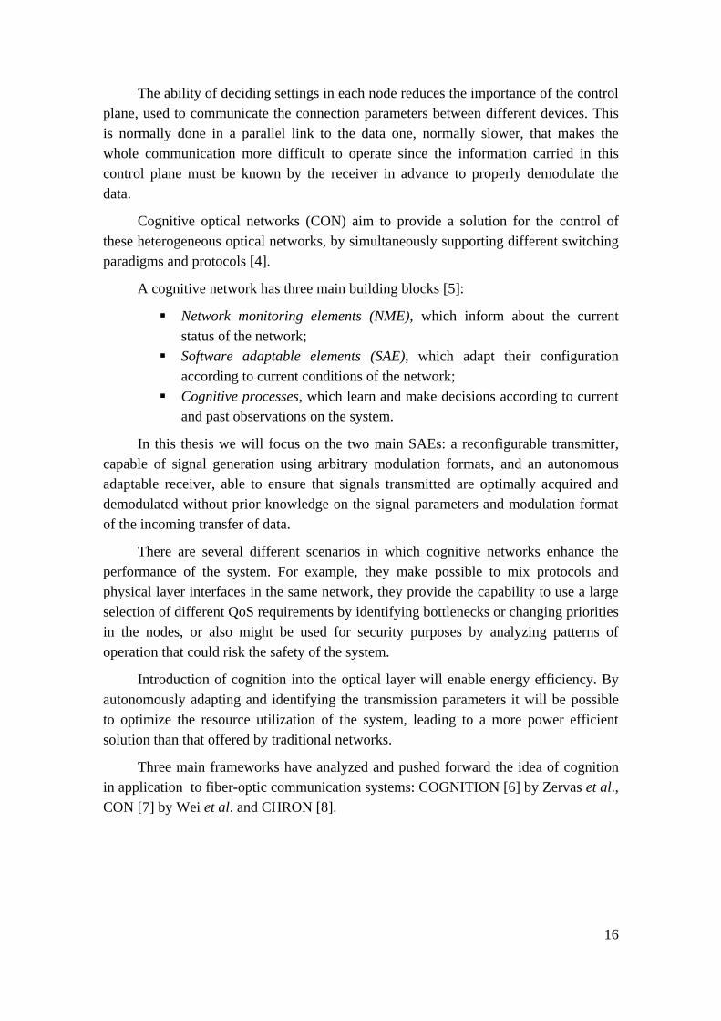
A cognitive network has three main building blocks [5]:

Network monitoring elements (NME), which inform about the current

status of the network;

Software adaptable elements (SAE), which adapt their configuration

according to current conditions of the network;

Cognitive processes, which learn and make decisions according to current

and past observations on the system.

In this thesis we will focus on the two main SAEs: a reconfigurable transmitter,

capable of signal generation using arbitrary modulation formats, and an autonomous

adaptable receiver, able to ensure that signals transmitted are optimally acquired and

demodulated without prior knowledge on the signal parameters and modulation format

of the incoming transfer of data.

There are several different scenarios in which cognitive networks enhance the

performance of the system. For example, they make possible to mix protocols and

physical layer interfaces in the same network, they provide the capability to use a large

selection of different QoS requirements by identifying bottlenecks or changing priorities

in the nodes, or also might be used for security purposes by analyzing patterns of

operation that could risk the safety of the system.

Introduction of cognition into the optical layer will enable energy efficiency. By

autonomously adapting and identifying the transmission parameters it will be possible

to optimize the resource utilization of the system, leading to a more power efficient

solution than that offered by traditional networks.

Three main frameworks have analyzed and pushed forward the idea of cognition

in application to fiber-optic communication systems: COGNITION [6] by Zervas et al.,

CON [7] by Wei et al. and CHRON [8].

17

Cognitive optical networks(CON)

Performance monitoring

Cognitive processes

Software adaptability

Figure 1.2. Interaction between different elements in a cognitive network.

1.2 Problem statement

With the advent of highly reconfigurable networks capable of adapting the

modulation format of the conveyed signal to the conditions of the link, seems very

important to have a mechanism to autonomously detect the characteristics of the signal

at the receiver side without any extra information, i.e. reducing the importance of a

control plane to send control commands.

In particular, it is very important to detect correctly the modulation format used in

the communication in order to be able to demodulate it without any prior information. It

also helps for Modulation Format Opaque algorithms, like equalization, which work

more effectively when the modulation format is known in advance. This functionality is

known as Modulation Format Recognition (MFR) [9].

MFR has been extensively explored for wireless applications in the field called

‘cognitive radio’ [10] with applications ranging from access networks to military

networks [11], where the goal is to optimize the spectrum utilization by using the most

optimal modulation format given the channel conditions. However it has not been much

researched in optical networks until very recently due to conventionally static nature of

these networks.

One can think of modulation format recognition in several contexts. An

immediate application is Optical Burst Switching (OBS) for heterogeneous networks

where the connections are turned up and down very fast. The need for rapid connection

setups motivates the employment of MFR as the use of the control plane and human

18

operation would noticeably slow down the operation of the whole system. It also helps

to decrease the overhead produced when many connections are initialized.

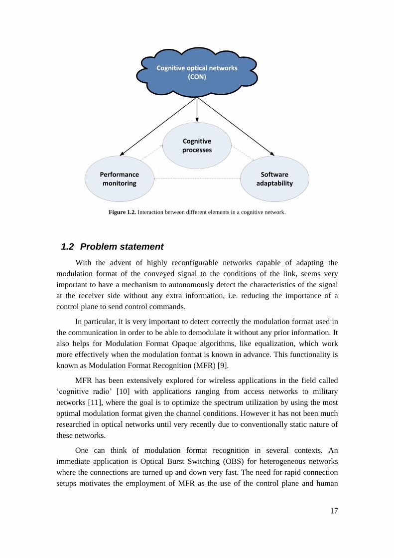
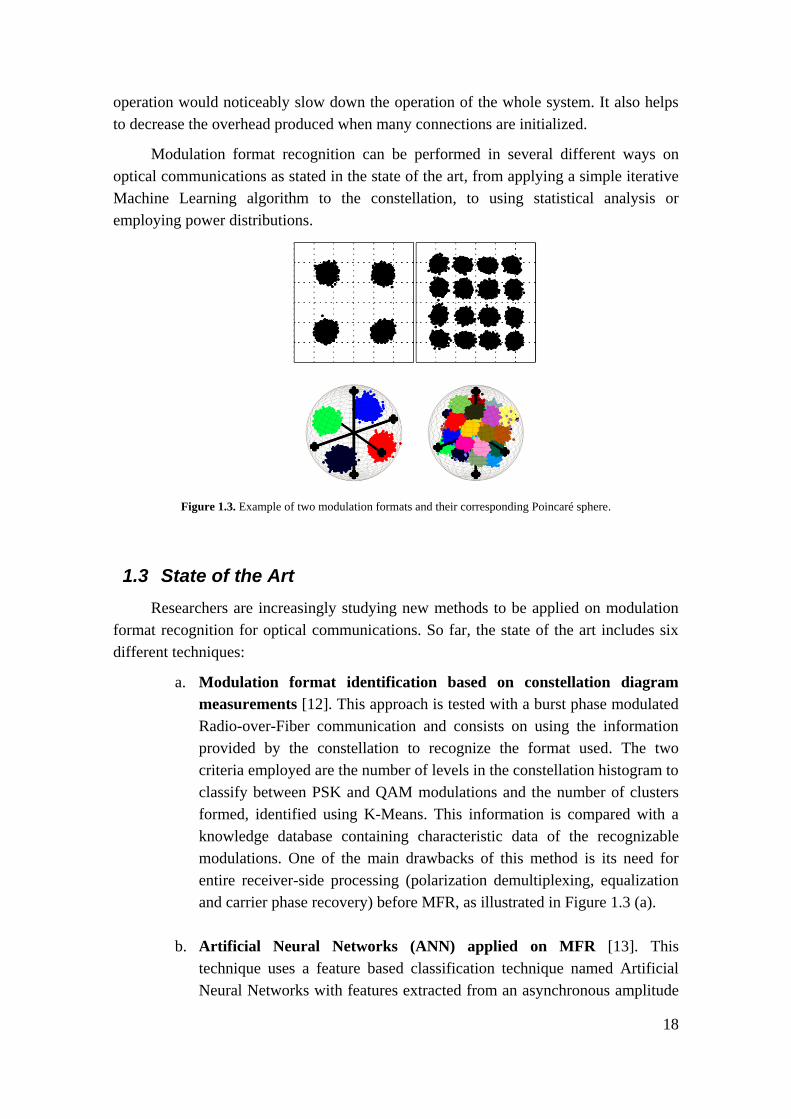
Modulation format recognition can be performed in several different ways on

optical communications as stated in the state of the art, from applying a simple iterative

Machine Learning algorithm to the constellation, to using statistical analysis or

employing power distributions.

Figure 1.3. Example of two modulation formats and their corresponding Poincaré sphere.

1.3 State of the Art

Researchers are increasingly studying new methods to be applied on modulation

format recognition for optical communications. So far, the state of the art includes six

different techniques:

a. Modulation format identification based on constellation diagram

measurements [12]. This approach is tested with a burst phase modulated

Radio-over-Fiber communication and consists on using the information

provided by the constellation to recognize the format used. The two

criteria employed are the number of levels in the constellation histogram to

classify between PSK and QAM modulations and the number of clusters

formed, identified using K-Means. This information is compared with a

knowledge database containing characteristic data of the recognizable

modulations. One of the main drawbacks of this method is its need for

entire receiver-side processing (polarization demultiplexing, equalization

and carrier phase recovery) before MFR, as illustrated in Figure 1.3 (a).

b. Artificial Neural Networks (ANN) applied on MFR [13]. This

technique uses a feature based classification technique named Artificial

Neural Networks with features extracted from an asynchronous amplitude

19

histogram (AAH) to identify the modulation format. It works with direct

detection and it suffers from the need for prior training.

c. Modulation format recognition with high-order statistics (HOS) in

Stokes space [14]. This MFR is performed in Stokes space. Firstly, a main

classification between 16QAM and the other possible formats (OOK,

BPSK, and QPSK) is done using a variational learning algorithm. The

discrimination between these three latter modulations consists on

evaluating signal cumulants on the 2D projection of the Stokes space

constellation and, by considering a Gaussian Mixture Model (GMM),

clustering this projection with a hierarchical clustering algorithm. Figure

1.3 (b) shows the position within the DSP flow where the MFR is applied.

d. Stokes space-based optical MFR with a machine learning technique

[15]. This approach considers the Stokes space representation of the

signal, where each modulation format shows a different number of

clusters. A clustering method is used to determine this number of clusters

and hence the modulation format of the incoming signal. The algorithm

chosen is a variation of Expectation Maximization, a commonly used

Machine Learning technique. This method allows for MFR at an early

stage in the receiver, as displayed in Figure 1.3 (c); does not require

training and provides valuable information for modulation format

dependent methods, like equalization.

e. Power distribution based MFR for digital coherent receivers [16].

Modulation formats are recognized by identifying special features from the

received signal power distribution. Although this technique produces very

good results comparing to the FEC limit, the features extracted from the

power distribution depend on the OSNR, which requires monitoring, and

thus, the knowledge of the modulation in advance. The position in the DSP

flow of a coherent receiver is shown in Figure 1.4 (d).

f. Modulation format identification using physical layer characteristics

[17]. The technique tested distinguishes between 15 possible single-

polarized modulations by extracting information from the complex electric

field magnitude histogram. Differentiation between different formats is

done in separate stages by comparing measurements taken directly from

the magnitude of the electric field. This procedure is tested with WDM

signals with 40000 samples. Figure 1.4 (e) shows the coherent receiver

DSP flow of this approach.

20

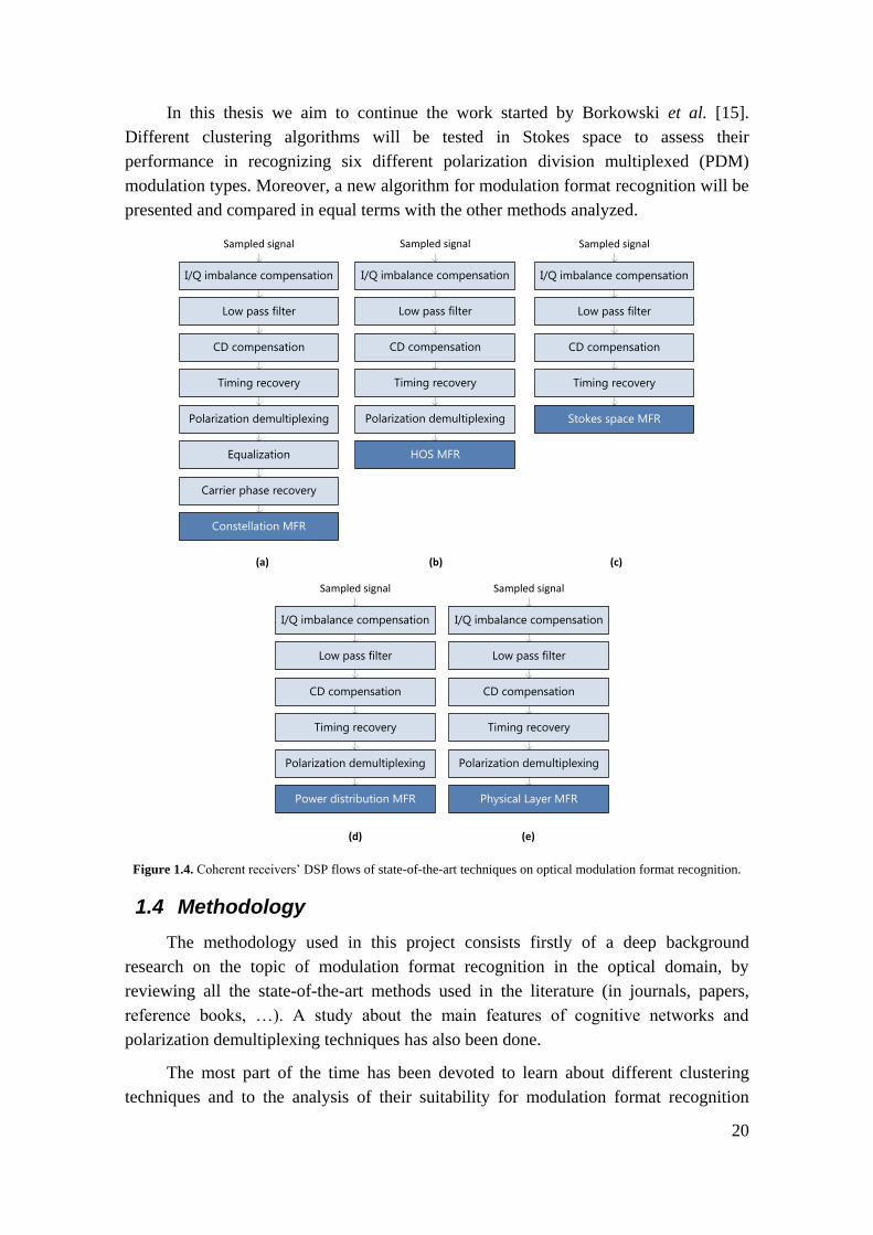
In this thesis we aim to continue the work started by Borkowski et al. [15].

Different clustering algorithms will be tested in Stokes space to assess their

performance in recognizing six different polarization division multiplexed (PDM)

modulation types. Moreover, a new algorithm for modulation format recognition will be

presented and compared in equal terms with the other methods analyzed.

I/Q imbalance compensation

Low pass filter

CD compensation

Timing recovery

Polarization demultiplexing

Equalization

Carrier phase recovery

Sampled signal

Constellation MFR

I/Q imbalance compensation

Low pass filter

CD compensation

Timing recovery

Polarization demultiplexing

HOS MFR

Sampled signal

I/Q imbalance compensation

Low pass filter

CD compensation

Timing recovery

Sampled signal

Stokes space MFR

I/Q imbalance compensation

Low pass filter

CD compensation

Timing recovery

Polarization demultiplexing

Sampled signal

Power distribution MFR

I/Q imbalance compensation

Low pass filter

CD compensation

Timing recovery

Polarization demultiplexing

Sampled signal

Physical Layer MFR

(a) (b) (c)

(d) (e)

Figure 1.4. Coherent receivers’ DSP flows of state-of-the-art techniques on optical modulation format recognition.

1.4 Methodology

The methodology used in this project consists firstly of a deep background

research on the topic of modulation format recognition in the optical domain, by

reviewing all the state-of-the-art methods used in the literature (in journals, papers,

reference books, …). A study about the main features of cognitive networks and

polarization demultiplexing techniques has also been done.

The most part of the time has been devoted to learn about different clustering

techniques and to the analysis of their suitability for modulation format recognition

21

purposes. The implementation of the algorithms has been done using the software

MATLAB.

Finally, the different techniques have been compared entirely by simulation in

three categories analyzing their performance, reliability and complexity.

1.5 Contributions

After carefully reviewing the state-of-the-art, with this thesis we are presenting

the first comparison of clustering algorithms in application to modulation format

recognition in fiber-optic networks so far in the literature. Six different techniques (K-

Means, Expectation Maximization, DBSCAN, OPTICS, Spectral Clustering and

Gravitational Clustering) have been contrasted in terms of their OSNR performance,

accuracy and complexity to assess their feasibility in a real working environment.

Furthermore, we are introducing a novel algorithm for identifying the modulation

format, solely from the input data set, without assuming any particular model for the

data. Its performance has been compared with the other algorithms in the same three

categories yielding some promising results to be further examined.

1.6 Thesis outline

The structure of this document is organized as follows. In Chapter 2, a brief

introduction to polarization demultiplexing and a more detailed explanation about

Stokes space are presented. Some ideas regarding the representation of states of

polarization in the Poincaré sphere are also given.

Chapter 3 introduces Machine Learning by giving an overall view of all available

techniques and their most popular applications. Focusing more on clustering, six

different algorithms are described: K-Means, Expectation Maximization, DBSCAN,

OPTICS, Spectral Clustering and Gravitational Clustering. Finally, two methods to

analyze the clustering outcomes are mentioned.

Chapter 4 is devoted to describe the novel proposed algorithm in detail, specially

focusing in the characteristics of the signals used to identify them and mentioning the

advantages introduced.

In Chapter 5, after stating the simulation setup used to contrast the methods, the

results obtained are assessed in terms of OSNR performance, accuracy and complexity.

The presented algorithm is also compared in these three categories.

Finally, in chapter 6, we summarize the main conclusions of the work done and

suggest some lines on future work.

22

23

2 Polarization demultiplexing

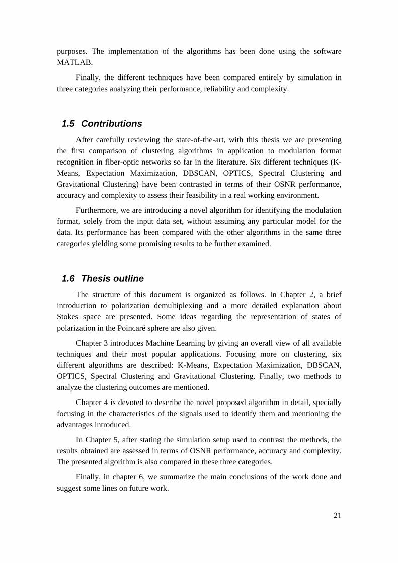
Polarization multiplexing is a type of optical transmissions that uses two

orthogonal polarization states, as shown in Figure 2.1, to transmit two different optical

signals at the same wavelength. It is a widely used method to double the spectral

efficiency.

Both polarization states can be excited independently and, ideally, would

propagate separately. However, the state of polarization (SOP) rotates along the fiber

and this causes the signal to arrive misaligned to the receiver, with both states mixed.

This is mainly a consequence of birefringence, which is the optical property by which

materials show a different refractive index depending on the polarization and direction

of light. Other fiber impairments, like polarization mode dispersion (PMD) –

polarization states travel at different speeds –, differential group delay (DGD) –

difference in propagation time between X and Y polarization states – or polarization

dependent losses (PDL) – difference in losses between both polarization states – are

also responsible for the SOP rotation.

In this scenario, a demultiplexing process is required in order to recover the

original transmitted optical signal and, therefore, the information sent. At the receiver,

the incoming signal is split into two orthogonal optical waves by the polarization beam

splitter (PBS), with a system of coordinates different from that of the transmitter. Thus,

each of the two orthogonal optical signals at the receiver is actually a linear combination

of the transmitted optical waves.

EY

EX

Figure 2.1. Orthogonal polarization states

24

To perform polarization demultiplexing, several different techniques exist, such as

the commonly used constant modulus algorithm (CMA). Due to the misalignment in

polarization states introduced by the fiber, simple modulation schemes can be observed

as multi-level signals at the receiver side. To avoid this, CMA introduces the idea of

enforcing constant modulus to the received data in order to properly demultiplex the

signal, by mapping resulting symbols with expected symbols. This is true only for

typical modulation formats like phase-shift keying (PSK), where the modulus is

constant for all symbols. A variation of this algorithm, radius directed equalization with

multiple modulus algorithm (RDE-MMA), considers several levels to overcome this

problem, allowing to deal with more advanced modulation formats.

Polarization demultiplexing in Stokes space is another method for the same

purpose, with the advantage it does not require knowledge of the modulation format and

it is faster in convergence. Therefore, working in Stokes space is very suitable for

Modulation Format Recognition purposes.

2.1 Polarization demultiplexing in Stokes space

Any state of polarization of a polarized lightwave can be formally described

through the Stokes parameters, and represented unequivocally with a different vector

orientation in Stokes space. Given an arbitrary plane defined by �⃗� and �⃗�, normal to the

propagation axis of the fiber, 𝑧, any electromagnetic field can be described easily as

shown in (2.1), where 𝑎𝑥 and 𝑎𝑦 are the amplitudes, and 𝜙𝑥 and 𝜙𝑦 are the phases of the

two orthogonal components.

where

�⃗⃗� = 𝑒𝑥�⃗� + 𝑒𝑦�⃗�

𝑒𝑥 = 𝑎𝑥𝑒𝑗(𝜔𝑡+𝜙𝑥)

𝑒𝑦 = 𝑎𝑦𝑒𝑗(𝜔𝑡+𝜙𝑦)

(2.1)

Jones calculus is a simple formalism introduced by R. Clark Jones (1941) for

describing polarized light in vector format. Moreover, linear optical elements can also

be represented by Jones matrices. The previous equation, (2.1), can be expressed in

terms of Jones vectors as shown in (2.2), where the first term 1

√2 is used for

normalization.

𝐸 =1

√2(𝑒𝑥𝑒𝑦) =

1

√2 (𝑎𝑥𝑒

𝑗(𝜔𝑡+𝜙𝑥)

𝑎𝑦𝑒𝑗(𝜔𝑡+𝜙𝑦)

) (2.2)

25

The effect of an assumed ideal optical fiber can be modelled by means of a unitary

Jones matrix independent of the optical frequency as described in (2.3). The unitary

condition states that the determinant of the matrix is 1, and this makes any orthogonal

wave to preserve its orthogonality through the fiber. Thus, to recover the initial

alignment of the signal it is necessary to compute the inverse matrix 𝐻−1.

𝐻 = (𝑎 𝑏−𝑏∗ 𝑎∗

) (2.3)

For example, launching the polarization state 𝐽 = (1, 0)𝑇 causes to have 𝐽′ =

(𝑎, −𝑏∗) at the end of the fiber. Applying 𝐻−1 to this signal yields the initial Jones

vector transmitted, since |𝑎|2 + |𝑏|2 = det(𝐻) = 1. The derivation is shown

mathematically in (2.4). We successfully recover the initially transmitted data.

𝐽𝑟𝑒𝑐 = 𝐻−1[ 𝐻 𝐽𝑡𝑥 ] = (

𝑎∗ −𝑏𝑏∗ 𝑎

) [(𝑎 𝑏−𝑏∗ 𝑎∗

) (1

0)] =

= (|𝑎|2 + |𝑏|2

𝑎𝑏∗ − 𝑏∗𝑎) = (

1

0)

(2.4)

We have seen that only by identifying the polarization states of the signal at the

receiver it is possible to construct the inverse matrix 𝐻−1 and thus the original wave.

The equations in (2.5) define the Stokes parameters in terms of received data in

Jones vector form. Stokes parameters were first introduced by Sir George Gabriel

Stokes in 1852, and allow to represent any state of polarized light (even unpolarized),

unlike Jones vector which only allows polarized light. They can be derived from the

transmitted intensities when the beam is passed through different degree polarizers [18].

𝑺 = (

𝑆0𝑆1𝑆2𝑆3

) =1

2

(

𝑒𝑥𝑒𝑥∗ + 𝑒𝑦𝑒𝑦

∗

𝑒𝑥𝑒𝑥∗ − 𝑒𝑦𝑒𝑦

∗

𝑒𝑥∗𝑒𝑦 + 𝑒𝑥𝑒𝑦

∗

−𝑗𝑒𝑥∗𝑒𝑦 + 𝑗𝑒𝑥𝑒𝑦

∗

)

=1

2

(

𝑎𝑥2 + 𝑎𝑦

2

𝑎𝑥2 − 𝑎𝑦

2

2𝑎𝑥𝑎𝑦 cos(𝜙𝑦 − 𝜙𝑥)

2𝑎𝑥𝑎𝑦sin (𝜙𝑦 − 𝜙𝑥) )

(2.5)

In (2.5) Stokes parameters are shown without normalizing, which is generally

done with respect to 𝑆0. We can also note that the parameters are independent of the

carrier frequency 𝜔 due to they operate in interpolarization differences. For the same

reason, they are also independent of the polarization mixing and the phase offset.

Each parameter conveys different information:

𝑆0 represents the total power of the light beam

𝑆1 represents 0º linear polarized light

𝑆2 represents 45º linear polarized light

𝑆3 represents circularly polarized light

26

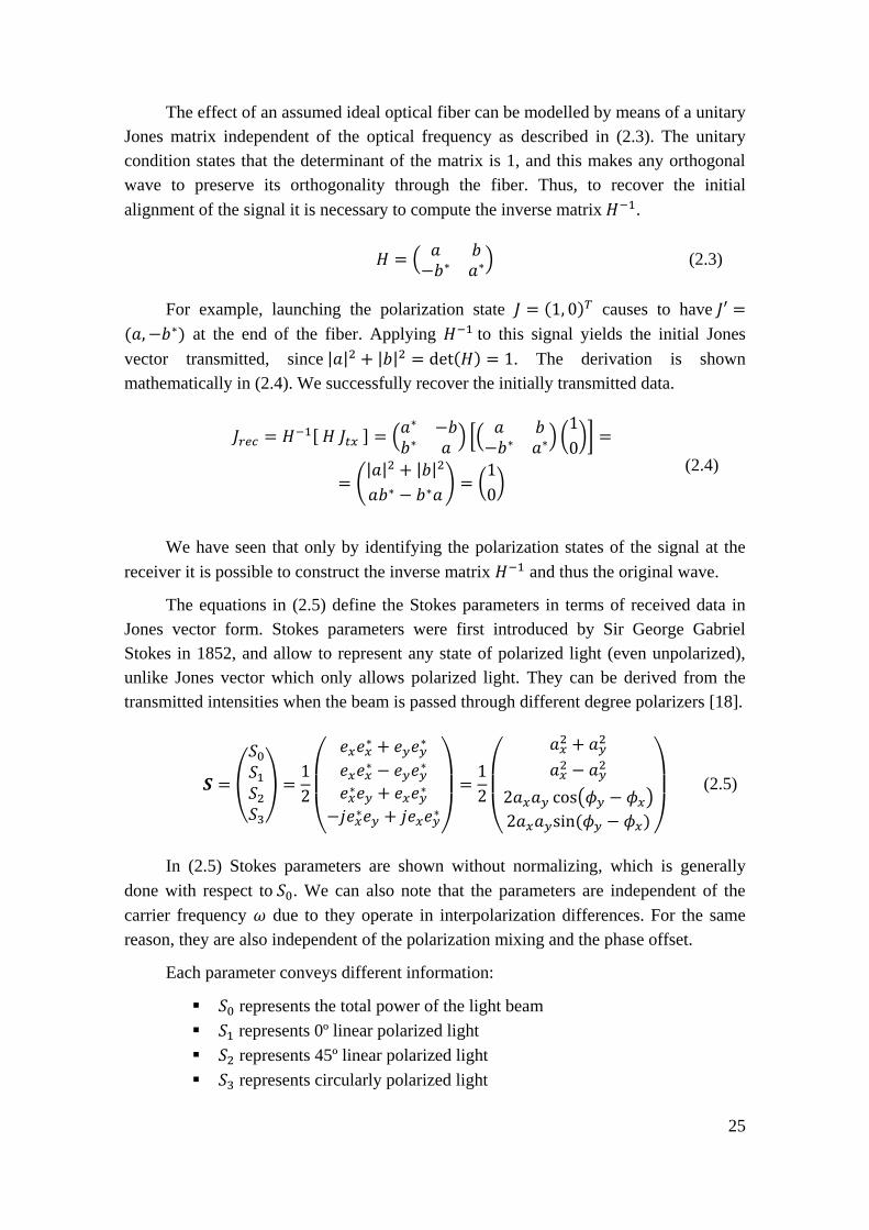
Figure 2.2. Different PDM formats constellations (top) with their corresponding Stokes space representation in the

Poincaré sphere for (a) PDM BPSK, (b) PDM QPSK, (c) PDM 8-PSK, (d) PDM star 8-QAM, (e) PDM 12-QAM, (f)

PDM 16-QAM.

The three components (𝑆1, 𝑆2, 𝑆3)𝑇 represent the polarization state in the three

dimensional space, which can be visualized on the Poincaré sphere. An explanation why

any modulation format can be represented in a lens-like object in Stokes space can be

found in [19]. Figure 2.2 shows the constellation for the different polarization division

multiplexed modulation formats considered in this thesis and their corresponding Stokes

space representation in the Poincaré sphere.

Each modulation format in Stokes space, as shown in Figure 2.2, shows a

different signature, i.e. number of clusters or groups of points, which can be used to

identify the modulation used in each communication.

Polarization demultiplexing in Stokes space is robust in front of fiber impairments

such as polarization mode dispersion (PMD), polarization dependent losses (PDL) and

chromatic dispersion (CD) [19].

2.2 Representation of Stokes parameters in the Poincaré

sphere

The Poincaré sphere was first conceived by Henri Poincaré in 1892. It is a

geometrical representation that allows visualizing any polarization state in a unit sphere

uniquely. A detailed analysis of it is beyond the scope of this document but few key

points are stated [18].

Each point describing a state of polarization is represented by a point within or on

the surface of a unit sphere centered on a (x,y,z) Cartesian coordinate system. The

coordinates of the point are the state of polarization corresponding Stokes parameters.

The distance from the coordinate origin to the point symbolizes the degree of

polarization the light has, with 0 meaning unpolarized (point at the centre of the sphere)

and 1 meaning totally polarized (point at the surface of the sphere). Following this

explanation, points close to each other in the Poincaré sphere have very similar

polarization states.

27

HorizontalHorizontal

Vertical

+45º

linear

-45º

linear

-45º

linear

Right circular

Left Circular

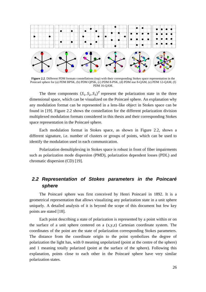
Figure 2.3. Illustration of the Poincaré sphere. The evolution of states of polarization along the sphere is depicted.

As we can see in Figure 2.3, in the equator of the sphere we can observe linear

polarizations, while in the poles we find circular polarizations. In the intermediate

positions between the equator and the poles there are the elliptical states, with the

northern hemisphere corresponding to right-hand polarized travelling waves and the

southern hemisphere corresponding to left-hand elliptical polarized states. Opposite

points on the sphere correspond to totally opposed polarizations.

28

29

3 Machine Learning

Machine Learning is the field of study that intends to give the computers or the

machines the ability to learn from data without being explicitly programmed and act

according to this information learnt [20]. It is considered a branch within Artificial

Intelligence, which comprises the idea of giving human-like intelligence to software-

defined machines.

The range of applications of Machine Learning is very broad including:

Prediction, where some current variables outputs are computed according

to prior obtained results of the same variables. One area where prediction

is applied is to make weather forecasts, for example.

Classification, where given an input point the algorithm tries to classify it

into one of the groups of the model previously defined. It might be used to

build classifiers for spam or fraud detection for instance.

Pattern recognition, with applications in many fields such as text

recognition (OCR), object recognition for computer vision, medicine

(ECG measurements), face recognition, etc.

Recommender platforms, which intend to predict the preference of a user

with respect to a certain product, based on latest purchases or liked items.

They have become extremely popular recently, with the exponential

growth of Internet advertising companies or Amazon-like websites.

Data mining, where the goal is to extract valuable information (patterns)

out of large data sets. It is a widely used term to refer to many

applications, with search engines and customer data extraction being two

of the most popular.

The algorithms within Machine Learning can be classified into two different

categories depending on the sort of information they are given, which is called data set

or training set:

Supervised learning: This kind of methods uses labelled information to feed the

system, i.e. the outcome of the algorithm for certain variable values is provided as

an input. For example, imagine a system that aims to classify mail into a spam

folder and a non-spam folder. In this case, the algorithm would be given some

examples of spam and non-spam mails correctly classified beforehand.

30

It is possible to further categorize supervised learning algorithms into two different

groups: regression and classification. On one hand, regression consists on

predicting continuous values while on the other hand, classification only outputs

discrete values.

Unsupervised learning: Unsupervised learning algorithms are given data which is

unlabelled, and the main goal is to separate it into different groups of points, also

called clusters, based on similarities between them. It also receives the more popular

name of clustering.

3.1 Clustering algorithms

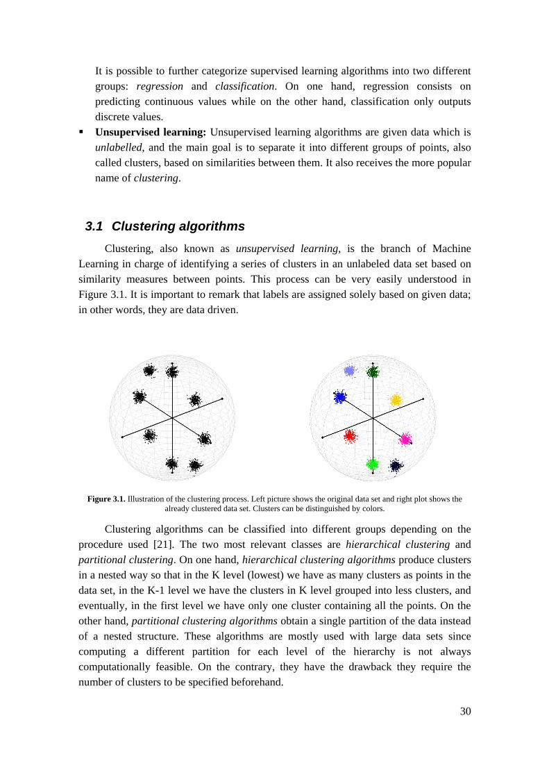
Clustering, also known as unsupervised learning, is the branch of Machine

Learning in charge of identifying a series of clusters in an unlabeled data set based on

similarity measures between points. This process can be very easily understood in

Figure 3.1. It is important to remark that labels are assigned solely based on given data;

in other words, they are data driven.

Figure 3.1. Illustration of the clustering process. Left picture shows the original data set and right plot shows the

already clustered data set. Clusters can be distinguished by colors.

Clustering algorithms can be classified into different groups depending on the

procedure used [21]. The two most relevant classes are hierarchical clustering and

partitional clustering. On one hand, hierarchical clustering algorithms produce clusters

in a nested way so that in the K level (lowest) we have as many clusters as points in the

data set, in the K-1 level we have the clusters in K level grouped into less clusters, and

eventually, in the first level we have only one cluster containing all the points. On the

other hand, partitional clustering algorithms obtain a single partition of the data instead

of a nested structure. These algorithms are mostly used with large data sets since

computing a different partition for each level of the hierarchy is not always

computationally feasible. On the contrary, they have the drawback they require the

number of clusters to be specified beforehand.

31

An important point in clustering algorithms is to define the similarity measure

between points. The most well-known similarity function is Euclidean distance, but an

arbitrary distance metric can be specified for each specific algorithm.

The algorithms described next are a selection covering from the most

representative to the most novel clustering algorithms. First, two of the most commonly

used clustering algorithms, K-Means and EM, are described. The list continues with two

density-based methods, DBSCAN and OPTICS, and finally we explain two completely

different techniques, Spectral Clustering and Gravitational Clustering.

3.1.1 K-Means

K-Means (MacQueen, 1967) is the simplest and most commonly used

unsupervised learning algorithm [22]. It belongs to partitional clustering, as shown in

Figure 3.2, and in its traditional form it uses the squared error criterion as distance

metric to compute similarity between points, although others can be specified. After

defining the search for a certain number of clusters K in the data set, the algorithm

decides an initial partition of clusters. Then, the method discovers the centroid (average

mean) of each cluster, and iteratively, assigns each point to the closest cluster and

recomputes the centroid of each cluster. The algorithm finishes when a certain

convergence criterion is met, usually set as a threshold on the cost function, which is the

average distance of each point to its assigned cluster.

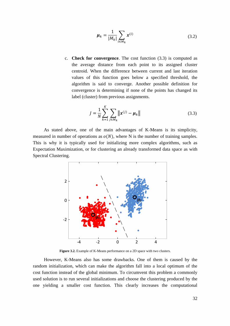
The algorithm runs the following procedure, given an initial data set defined

by {𝒙1, 𝒙2, … , 𝒙𝑁}. It is also schematically depicted in Figure 3.3.

I. Initial partition. The centroids of each cluster are defined by 𝝁1, … , 𝝁𝐾,

where each 𝝁𝑘 has the same dimension as the points in the data set. In the

initialization step, a first selection of centroids is chosen, normally by

taking random samples, although other initializations can also be applied.

II. Iteratively run these two steps until convergence is achieved:

a. Cluster assignment step. Each point is assigned to the cluster the

centroid of which is closest. For each point i in the data set, its

label is assigned as in (3.1).

𝑐(𝑖) = 𝑎𝑟𝑔 𝑚𝑖𝑛𝑘‖𝒙𝑖 − 𝝁𝑘 ‖ ∀𝑘 = 1:𝐾 (3.1)

b. Move centroids step. Each cluster centroid is recomputed

according to the current data set. Defining 𝑀𝑘 as the collection of

points’ indices that belong to cluster 𝑘, the centroid of each cluster

is computed using (3.2).

32

𝝁𝑘 =1

|𝑀𝑘|∑ 𝒙(𝑖)

𝑖∈𝑀𝑘

(3.2)

c. Check for convergence. The cost function (3.3) is computed as

the average distance from each point to its assigned cluster

centroid. When the difference between current and last iteration

values of this function goes below a specified threshold, the

algorithm is said to converge. Another possible definition for

convergence is determining if none of the points has changed its

label (cluster) from previous assignments.

𝐽 =1

𝑁∑ ∑‖𝒙(𝑗) − 𝝁𝑘‖

𝑗∈𝑀𝑘

𝐾

𝑘=1

(3.3)

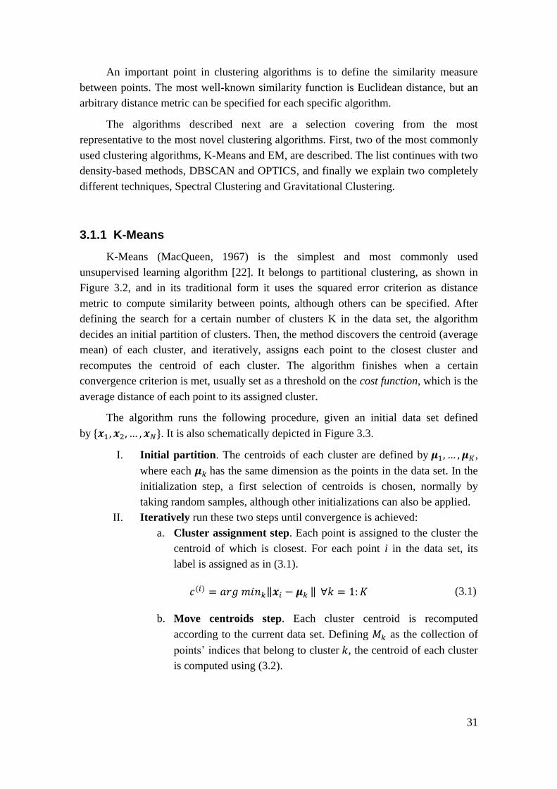
As stated above, one of the main advantages of K-Means is its simplicity,

measured in number of operations as 𝑜(𝑁), where N is the number of training samples.

This is why it is typically used for initializing more complex algorithms, such as

Expectation Maximization, or for clustering an already transformed data space as with

Spectral Clustering.

Figure 3.2. Example of K-Means performance on a 2D space with two clusters.

However, K-Means also has some drawbacks. One of them is caused by the

random initialization, which can make the algorithm fall into a local optimum of the

cost function instead of the global minimum. To circumvent this problem a commonly

used solution is to run several initializations and choose the clustering produced by the

one yielding a smaller cost function. This clearly increases the computational

-2

0

2

0 2 4-2-4

µ1

µ2

33

complexity but increases the reliability. Another popular problem presented by K-

Means is the need to previously specify the number of clusters, which in our case is the

desired outcome. This can be solved by running the algorithm with every number of

clusters targeted, each one corresponding to a different modulation format, and selecting

the one that provides better results in terms of some figure of merit like the cost function

or any other clustering indices such as Silhouette, which is further explained in Section

3.2. Finally, K-Means only allow a certain shape for clusters. For instance, if we had

two ring-shaped clusters, one inside the other, it would be impossible to separate them

using this algorithm.

Selection ofinitial partition with

#clusters = K

START

Cluster assignment

Recompute centroids

Convergence achieved?

No

Yes

END

Figure 3.3. K-Means flow chart.

3.1.2 Expectation Maximization (EM)

The Expectation Maximization algorithm (Dempster et al, 1977) can be seen as a

maximum-likelihood estimator with some latent variables, i.e. variables whose value is

unknown [23].

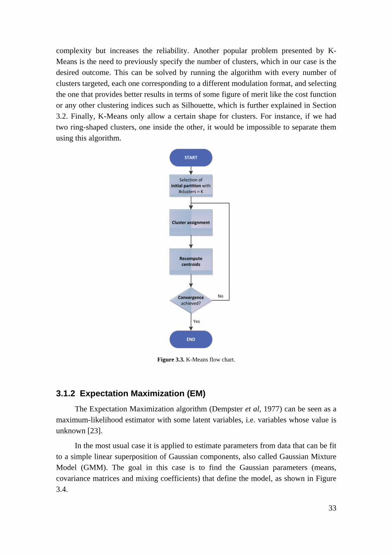
In the most usual case it is applied to estimate parameters from data that can be fit

to a simple linear superposition of Gaussian components, also called Gaussian Mixture

Model (GMM). The goal in this case is to find the Gaussian parameters (means,

covariance matrices and mixing coefficients) that define the model, as shown in Figure

3.4.

34

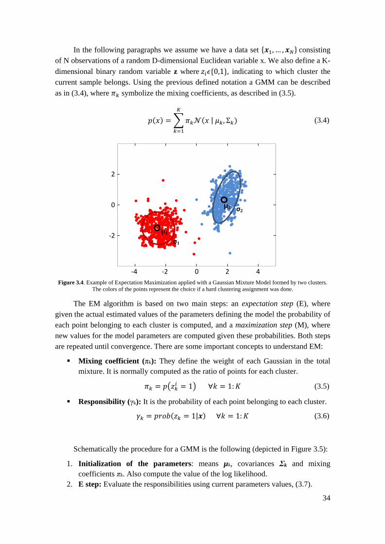
In the following paragraphs we assume we have a data set {𝒙1, … , 𝒙𝑁} consisting

of N observations of a random D-dimensional Euclidean variable x. We also define a K-

dimensional binary random variable z where 𝑧𝑖𝜖{0,1}, indicating to which cluster the

current sample belongs. Using the previous defined notation a GMM can be described

as in (3.4), where 𝜋𝑘 symbolize the mixing coefficients, as described in (3.5).

𝑝(𝑥) = ∑𝜋𝑘𝒩(𝑥 | 𝜇𝑘, Σ𝑘)

𝐾

𝑘=1

(3.4)

Figure 3.4. Example of Expectation Maximization applied with a Gaussian Mixture Model formed by two clusters.

The colors of the points represent the choice if a hard clustering assignment was done.

The EM algorithm is based on two main steps: an expectation step (E), where

given the actual estimated values of the parameters defining the model the probability of

each point belonging to each cluster is computed, and a maximization step (M), where

new values for the model parameters are computed given these probabilities. Both steps

are repeated until convergence. There are some important concepts to understand EM:

Mixing coefficient (πk): They define the weight of each Gaussian in the total

mixture. It is normally computed as the ratio of points for each cluster.

𝜋𝑘 = 𝑝(𝑧𝑘𝑖 = 1) ∀𝑘 = 1:𝐾 (3.5)

Responsibility (γk): It is the probability of each point belonging to each cluster.

𝛾𝑘 = 𝑝𝑟𝑜𝑏(𝑧𝑘 = 1|𝒙) ∀𝑘 = 1:𝐾 (3.6)

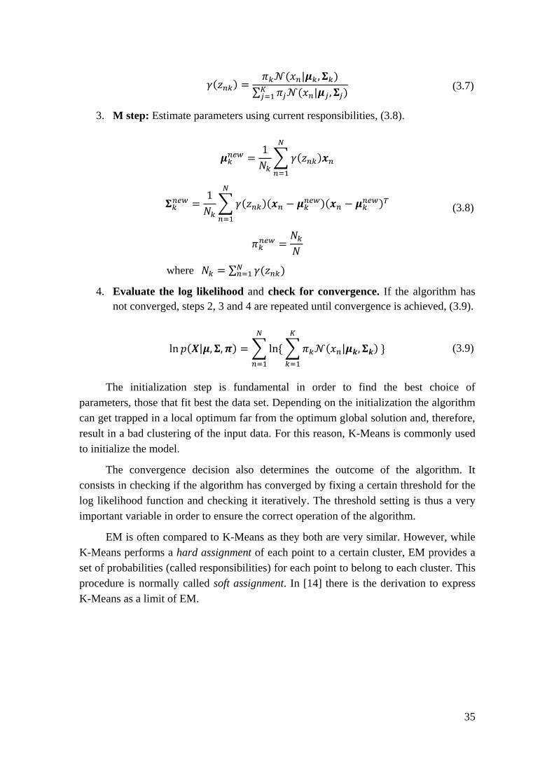
Schematically the procedure for a GMM is the following (depicted in Figure 3.5):

1. Initialization of the parameters: means µk, covariances Σk and mixing

coefficients πk. Also compute the value of the log likelihood.

2. E step: Evaluate the responsibilities using current parameters values, (3.7).

-2

0

2

0 2 4-2-4

µ1

µ2

σ1

σ2

35

𝛾(𝑧𝑛𝑘) =𝜋𝑘𝒩(𝑥𝑛|𝝁𝑘, 𝚺𝑘)

∑ 𝜋𝑗𝒩(𝑥𝑛|𝝁𝑗 , 𝚺𝑗)𝐾𝑗=1

(3.7)

3. M step: Estimate parameters using current responsibilities, (3.8).

𝝁𝑘𝑛𝑒𝑤 =

1

𝑁𝑘∑𝛾(𝑧𝑛𝑘)𝒙𝑛

𝑁

𝑛=1

𝚺𝑘𝑛𝑒𝑤 =

1

𝑁𝑘∑𝛾(𝑧𝑛𝑘)(𝒙𝑛 − 𝝁𝑘

𝑛𝑒𝑤)(𝒙𝑛 − 𝝁𝑘𝑛𝑒𝑤)𝑇

𝑁

𝑛=1

𝜋𝑘𝑛𝑒𝑤 =

𝑁𝑘𝑁

where 𝑁𝑘 = ∑ 𝛾(𝑧𝑛𝑘)𝑁𝑛=1

(3.8)

4. Evaluate the log likelihood and check for convergence. If the algorithm has

not converged, steps 2, 3 and 4 are repeated until convergence is achieved, (3.9).

ln 𝑝(𝑿|𝝁, 𝚺, 𝝅) = ∑ ln{ ∑𝜋𝑘𝒩(𝑥𝑛|𝝁𝒌, 𝚺𝒌)

𝐾

𝑘=1

}

𝑁

𝑛=1

(3.9)

The initialization step is fundamental in order to find the best choice of

parameters, those that fit best the data set. Depending on the initialization the algorithm

can get trapped in a local optimum far from the optimum global solution and, therefore,

result in a bad clustering of the input data. For this reason, K-Means is commonly used

to initialize the model.

The convergence decision also determines the outcome of the algorithm. It

consists in checking if the algorithm has converged by fixing a certain threshold for the

log likelihood function and checking it iteratively. The threshold setting is thus a very

important variable in order to ensure the correct operation of the algorithm.

EM is often compared to K-Means as they both are very similar. However, while

K-Means performs a hard assignment of each point to a certain cluster, EM provides a

set of probabilities (called responsibilities) for each point to belong to each cluster. This

procedure is normally called soft assignment. In [14] there is the derivation to express

K-Means as a limit of EM.

36

Initialization of parameters(µk, Σk, πk)

START

Expectation stepγ(znk)

Maximization step(µk

new, Σknew, πk

new)

Convergence achieved? No

Yes

END

Log likelihood evaluation

ln p(X|µ, Σ, π)

Figure 3.5. EM flow chart.

3.1.3 Density Based Spatial Clustering of Application with Noise

(DBSCAN)

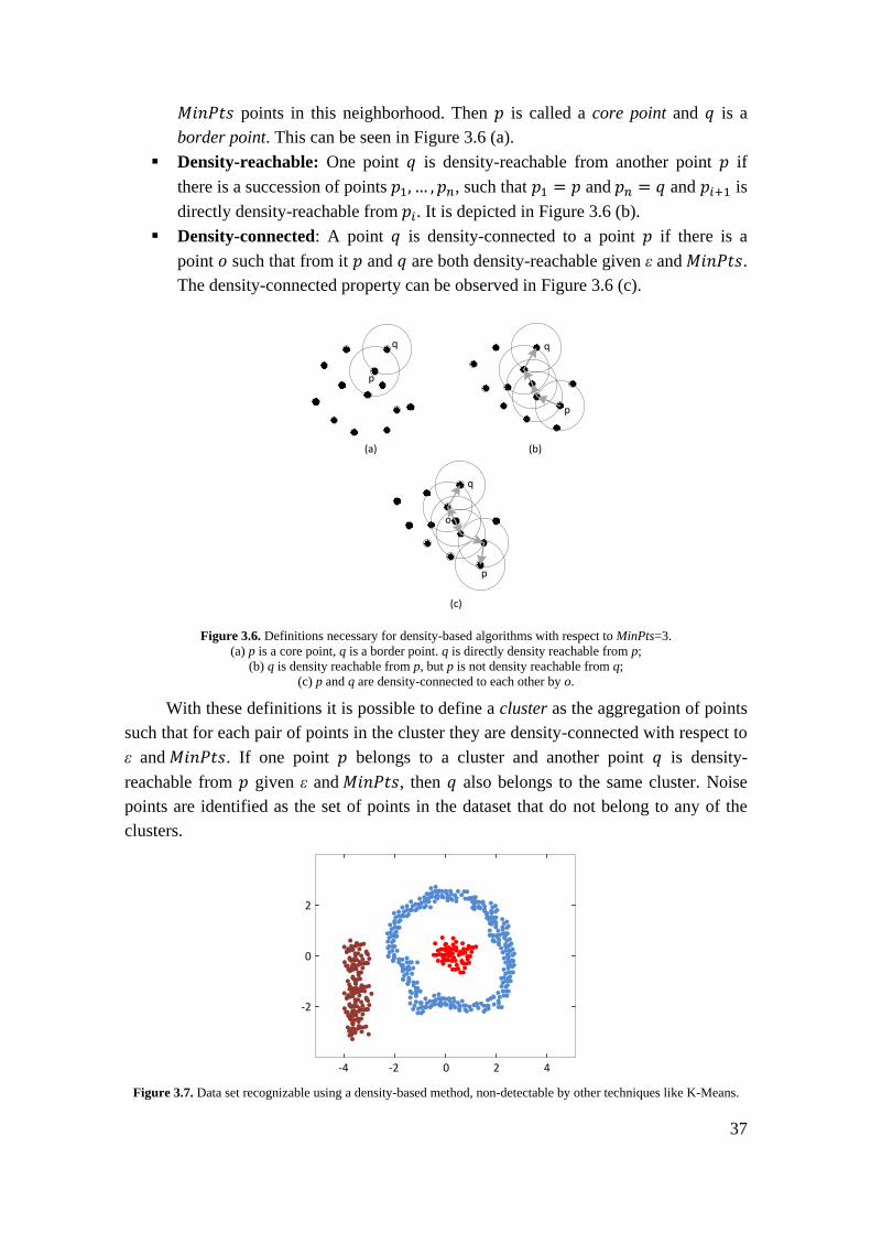
Some of the usual problems when dealing with clustering algorithms are: i) it is

often difficult to determine the input parameters to be used for a specific database; ii)

they are normally very computationally costly; and iii) they are restricted to only some

cluster shapes, as shown in Figure 3.7. The DBSCAN algorithm (Ester et al, 1996) is a

density-based technique that offers a solution to these three main problems [25].

The algorithm consists in identifying the clusters by referring to the density of the

database elements, with minimal knowledge of the domain by the user. Moreover, it

differentiates points of noise and reliable points to be included in a cluster.

To understand the procedure it is necessary to introduce some definitions before:

ε-neighborhood of a point: It comprises all the points within a distance below

than ε from the point.

Directly density-reachable: One point 𝑞 is directly density-reachable from

another point 𝑝 if 𝑞 belongs to the ε-neighborhood of 𝑝 and there are more than

37

𝑀𝑖𝑛𝑃𝑡𝑠 points in this neighborhood. Then 𝑝 is called a core point and 𝑞 is a

border point. This can be seen in Figure 3.6 (a).

Density-reachable: One point 𝑞 is density-reachable from another point 𝑝 if

there is a succession of points 𝑝1, … , 𝑝𝑛, such that 𝑝1 = 𝑝 and 𝑝𝑛 = 𝑞 and 𝑝𝑖+1 is

directly density-reachable from 𝑝𝑖. It is depicted in Figure 3.6 (b).

Density-connected: A point 𝑞 is density-connected to a point 𝑝 if there is a

point 𝑜 such that from it 𝑝 and 𝑞 are both density-reachable given ε and 𝑀𝑖𝑛𝑃𝑡𝑠.

The density-connected property can be observed in Figure 3.6 (c).

q

p

q

p

p

q

o

(a) (b)

(c)

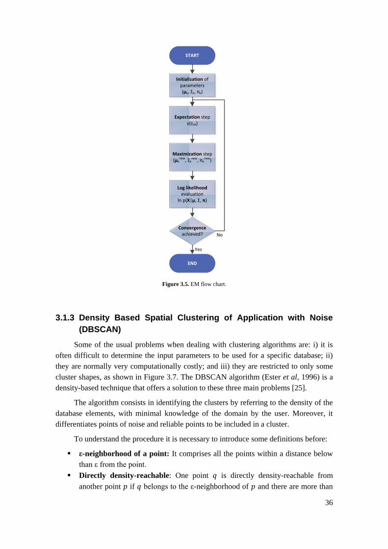
Figure 3.6. Definitions necessary for density-based algorithms with respect to MinPts=3.

(a) p is a core point, q is a border point. q is directly density reachable from p;

(b) q is density reachable from p, but p is not density reachable from q;

(c) p and q are density-connected to each other by o.

With these definitions it is possible to define a cluster as the aggregation of points

such that for each pair of points in the cluster they are density-connected with respect to

ε and 𝑀𝑖𝑛𝑃𝑡𝑠. If one point 𝑝 belongs to a cluster and another point 𝑞 is density-

reachable from 𝑝 given ε and 𝑀𝑖𝑛𝑃𝑡𝑠, then 𝑞 also belongs to the same cluster. Noise

points are identified as the set of points in the dataset that do not belong to any of the

clusters.

-2

0

2

0 2 4-2-4

Figure 3.7. Data set recognizable using a density-based method, non-detectable by other techniques like K-Means.

38

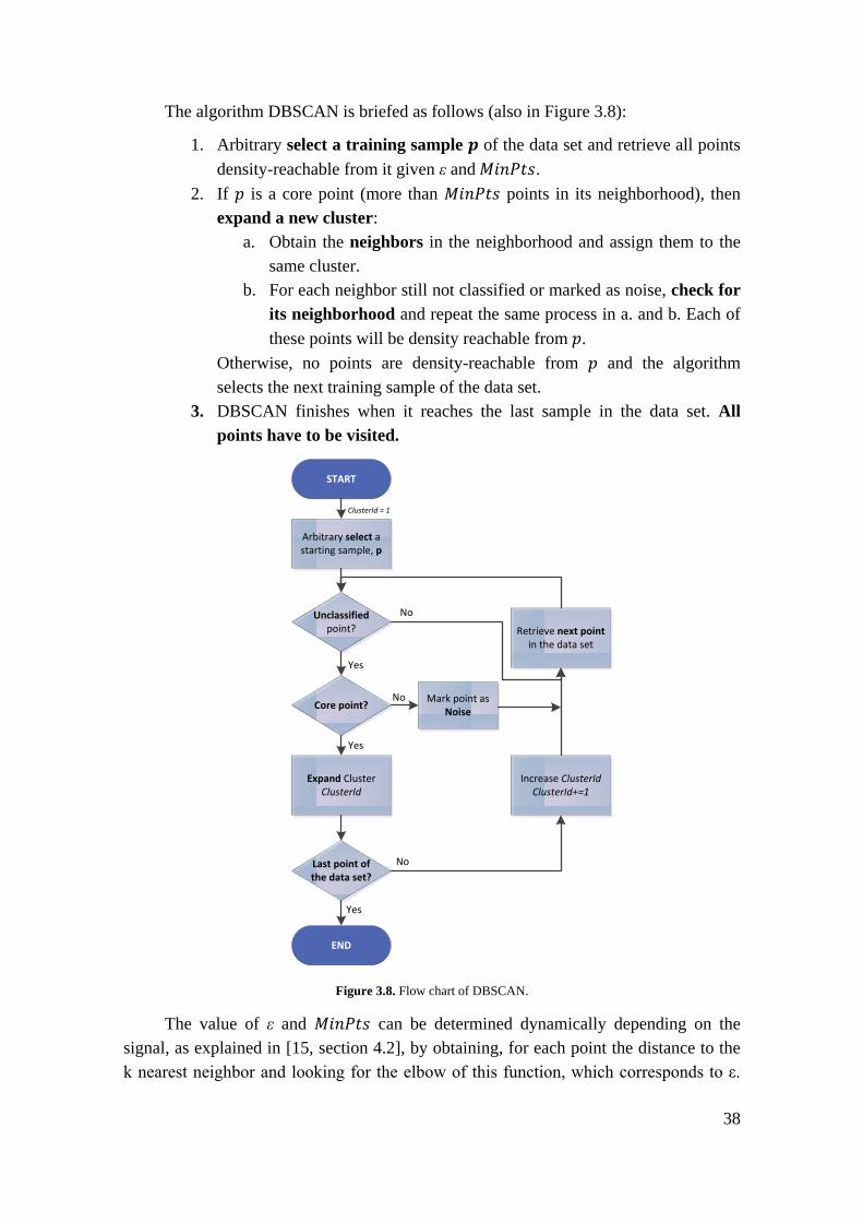
The algorithm DBSCAN is briefed as follows (also in Figure 3.8):

1. Arbitrary select a training sample 𝒑 of the data set and retrieve all points

density-reachable from it given ε and 𝑀𝑖𝑛𝑃𝑡𝑠.

2. If 𝑝 is a core point (more than 𝑀𝑖𝑛𝑃𝑡𝑠 points in its neighborhood), then

expand a new cluster:

a. Obtain the neighbors in the neighborhood and assign them to the

same cluster.

b. For each neighbor still not classified or marked as noise, check for

its neighborhood and repeat the same process in a. and b. Each of

these points will be density reachable from 𝑝.

Otherwise, no points are density-reachable from 𝑝 and the algorithm

selects the next training sample of the data set.

3. DBSCAN finishes when it reaches the last sample in the data set. All

points have to be visited.

Arbitrary select a starting sample, p

START

Expand Cluster ClusterId

ClusterId = 1

Unclassified point?

Last point of the data set?

Retrieve next point in the data set

Increase ClusterIdClusterId+=1

END

Core point?Mark point as

Noise

Yes

Yes

Yes

No

No

No

Figure 3.8. Flow chart of DBSCAN.

The value of ε and 𝑀𝑖𝑛𝑃𝑡𝑠 can be determined dynamically depending on the

signal, as explained in [15, section 4.2], by obtaining, for each point the distance to the

k nearest neighbor and looking for the elbow of this function, which corresponds to ε.

39

𝑀𝑖𝑛𝑃𝑡𝑠 may be computed by taking the average number of neighbors each point has at

distance ≤ 𝜀.

3.1.4 Ordering Points to Identify the Clustering Structure (OPTICS)

OPTICS (Ankerst et al, 1999) is another density-based clustering method, a more

generalized view of the DBSCAN algorithm [26]. It introduces the idea of, instead of

hard-assigning clusters, producing a special order of the database containing all the

valuable information to extract a certain clustering structure.

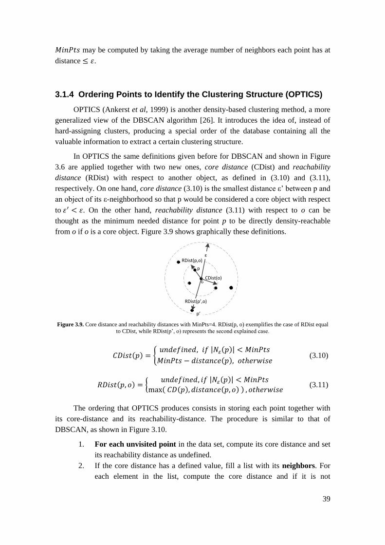
In OPTICS the same definitions given before for DBSCAN and shown in Figure

3.6 are applied together with two new ones, core distance (CDist) and reachability

distance (RDist) with respect to another object, as defined in (3.10) and (3.11),

respectively. On one hand, core distance (3.10) is the smallest distance ε’ between p and

an object of its ε-neighborhood so that p would be considered a core object with respect

to 𝜀′ < 𝜀. On the other hand, reachability distance (3.11) with respect to o can be

thought as the minimum needed distance for point p to be directly density-reachable

from o if o is a core object. Figure 3.9 shows graphically these definitions.

Figure 3.9. Core distance and reachability distances with MinPts=4. RDist(p, o) exemplifies the case of RDist equal

to CDist, while RDist(p’, o) represents the second explained case.

𝐶𝐷𝑖𝑠𝑡(𝑝) = {𝑢𝑛𝑑𝑒𝑓𝑖𝑛𝑒𝑑, 𝑖𝑓 |𝑁𝜀(𝑝)| < 𝑀𝑖𝑛𝑃𝑡𝑠

𝑀𝑖𝑛𝑃𝑡𝑠 − 𝑑𝑖𝑠𝑡𝑎𝑛𝑐𝑒(𝑝), 𝑜𝑡ℎ𝑒𝑟𝑤𝑖𝑠𝑒 (3.10)

𝑅𝐷𝑖𝑠𝑡(𝑝, 𝑜) = {𝑢𝑛𝑑𝑒𝑓𝑖𝑛𝑒𝑑, 𝑖𝑓 |𝑁𝜀(𝑝)| < 𝑀𝑖𝑛𝑃𝑡𝑠

max( 𝐶𝐷(𝑝), 𝑑𝑖𝑠𝑡𝑎𝑛𝑐𝑒(𝑝, 𝑜) ) , 𝑜𝑡ℎ𝑒𝑟𝑤𝑖𝑠𝑒 (3.11)

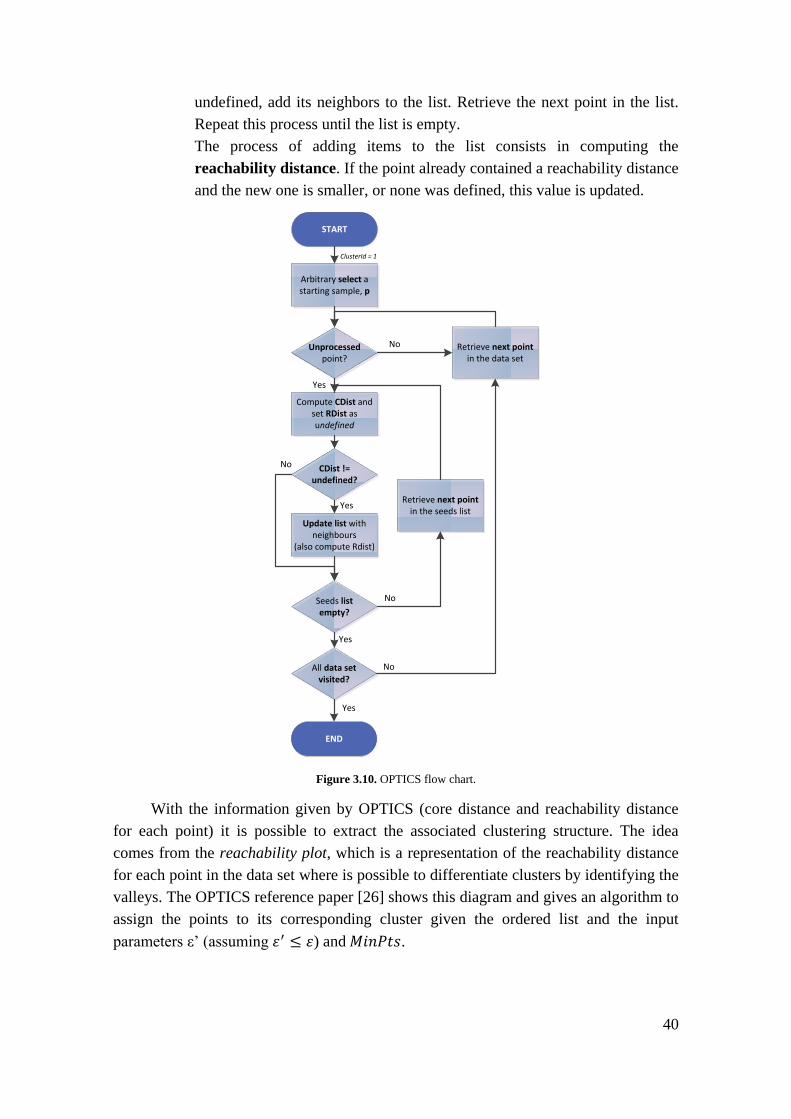
The ordering that OPTICS produces consists in storing each point together with

its core-distance and its reachability-distance. The procedure is similar to that of

DBSCAN, as shown in Figure 3.10.

1. For each unvisited point in the data set, compute its core distance and set

its reachability distance as undefined.

2. If the core distance has a defined value, fill a list with its neighbors. For

each element in the list, compute the core distance and if it is not

RDist(p’,o)

oCDist(o)

p’

p

RDist(p,o)ε

40

undefined, add its neighbors to the list. Retrieve the next point in the list.

Repeat this process until the list is empty.

The process of adding items to the list consists in computing the

reachability distance. If the point already contained a reachability distance

and the new one is smaller, or none was defined, this value is updated.

Arbitrary select a starting sample, p

START

ClusterId = 1

Unprocessed point?

END

Compute CDist and set RDist as undefined

CDist != undefined?

Update list with neighbours

(also compute Rdist)

Retrieve next point in the data set

Seeds list empty?

Retrieve next point in the seeds list

All data set visited?

No

No

Yes

No

Yes

No

Yes

Yes

Figure 3.10. OPTICS flow chart.

With the information given by OPTICS (core distance and reachability distance

for each point) it is possible to extract the associated clustering structure. The idea

comes from the reachability plot, which is a representation of the reachability distance

for each point in the data set where is possible to differentiate clusters by identifying the

valleys. The OPTICS reference paper [26] shows this diagram and gives an algorithm to

assign the points to its corresponding cluster given the ordered list and the input

parameters ε’ (assuming 𝜀′ ≤ 𝜀) and 𝑀𝑖𝑛𝑃𝑡𝑠.

41

3.1.5 Spectral Clustering

Spectral Clustering is one of the most recent clustering algorithms [27], [28]. It

offers some advantages in front of more traditional clustering techniques, as for instance

it does not require the assumption of a certain density function like EM, assuming a

Gaussian mixture model, and it is not vulnerable to local minima as K-Means.

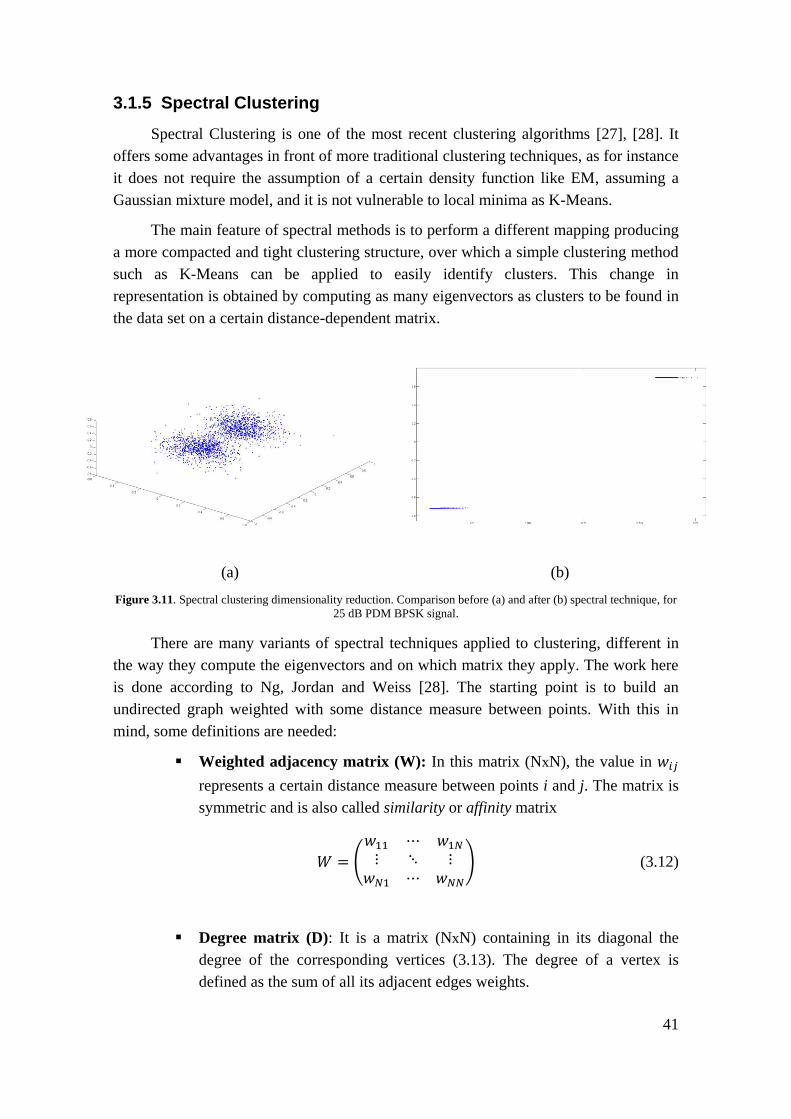
The main feature of spectral methods is to perform a different mapping producing

a more compacted and tight clustering structure, over which a simple clustering method

such as K-Means can be applied to easily identify clusters. This change in

representation is obtained by computing as many eigenvectors as clusters to be found in

the data set on a certain distance-dependent matrix.

(a) (b)

Figure 3.11. Spectral clustering dimensionality reduction. Comparison before (a) and after (b) spectral technique, for

25 dB PDM BPSK signal.

There are many variants of spectral techniques applied to clustering, different in

the way they compute the eigenvectors and on which matrix they apply. The work here

is done according to Ng, Jordan and Weiss [28]. The starting point is to build an

undirected graph weighted with some distance measure between points. With this in

mind, some definitions are needed:

Weighted adjacency matrix (W): In this matrix (NxN), the value in 𝑤𝑖𝑗

represents a certain distance measure between points i and j. The matrix is

symmetric and is also called similarity or affinity matrix

𝑊 = (

𝑤11 ⋯ 𝑤1𝑁⋮ ⋱ ⋮𝑤𝑁1 ⋯ 𝑤𝑁𝑁

) (3.12)

Degree matrix (D): It is a matrix (NxN) containing in its diagonal the

degree of the corresponding vertices (3.13). The degree of a vertex is

defined as the sum of all its adjacent edges weights.

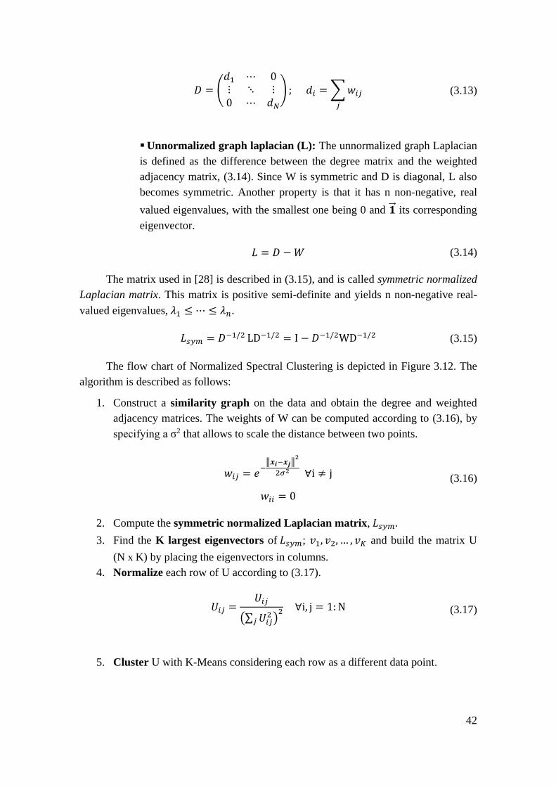
42

𝐷 = (𝑑1 ⋯ 0⋮ ⋱ ⋮0 ⋯ 𝑑𝑁

) ; 𝑑𝑖 =∑𝑤𝑖𝑗𝑗

(3.13)

Unnormalized graph laplacian (L): The unnormalized graph Laplacian

is defined as the difference between the degree matrix and the weighted

adjacency matrix, (3.14). Since W is symmetric and D is diagonal, L also

becomes symmetric. Another property is that it has n non-negative, real

valued eigenvalues, with the smallest one being 0 and �⃗⃗⃗� its corresponding

eigenvector.

𝐿 = 𝐷 −𝑊 (3.14)

The matrix used in [28] is described in (3.15), and is called symmetric normalized

Laplacian matrix. This matrix is positive semi-definite and yields n non-negative real-

valued eigenvalues, 𝜆1 ≤ ⋯ ≤ 𝜆𝑛.

𝐿𝑠𝑦𝑚 = 𝐷−1/2 LD−1/2 = I − 𝐷−1/2WD−1/2 (3.15)

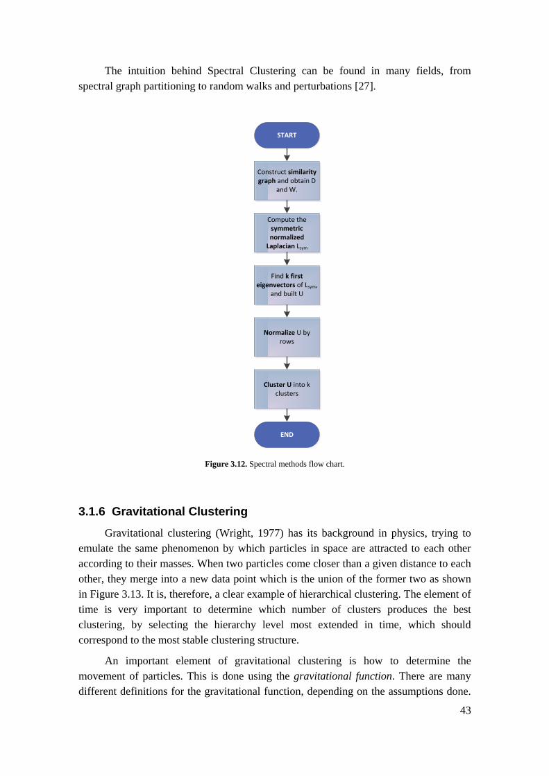
The flow chart of Normalized Spectral Clustering is depicted in Figure 3.12. The

algorithm is described as follows:

1. Construct a similarity graph on the data and obtain the degree and weighted

adjacency matrices. The weights of W can be computed according to (3.16), by

specifying a σ2 that allows to scale the distance between two points.

𝑤𝑖𝑗 = 𝑒−‖𝒙𝒊−𝒙𝒋‖

2

2𝜎2 ∀i ≠ j

𝑤𝑖𝑖 = 0

(3.16)

2. Compute the symmetric normalized Laplacian matrix, 𝐿𝑠𝑦𝑚.

3. Find the K largest eigenvectors of 𝐿𝑠𝑦𝑚; 𝑣1, 𝑣2, … , 𝑣𝐾 and build the matrix U

(N x K) by placing the eigenvectors in columns.

4. Normalize each row of U according to (3.17).

𝑈𝑖𝑗 =𝑈𝑖𝑗

(∑ 𝑈𝑖𝑗2

𝑗 )2 ∀i, j = 1: N (3.17)

5. Cluster U with K-Means considering each row as a different data point.

43

The intuition behind Spectral Clustering can be found in many fields, from

spectral graph partitioning to random walks and perturbations [27].

START

END

Construct similarity graph and obtain D

and W.

Compute the symmetric normalized

Laplacian Lsym

Find k first eigenvectors of Lsym,

and built U

Normalize U by rows

Cluster U into k clusters

Figure 3.12. Spectral methods flow chart.

3.1.6 Gravitational Clustering

Gravitational clustering (Wright, 1977) has its background in physics, trying to

emulate the same phenomenon by which particles in space are attracted to each other

according to their masses. When two particles come closer than a given distance to each

other, they merge into a new data point which is the union of the former two as shown

in Figure 3.13. It is, therefore, a clear example of hierarchical clustering. The element of

time is very important to determine which number of clusters produces the best

clustering, by selecting the hierarchy level most extended in time, which should

correspond to the most stable clustering structure.

An important element of gravitational clustering is how to determine the

movement of particles. This is done using the gravitational function. There are many

different definitions for the gravitational function, depending on the assumptions done.

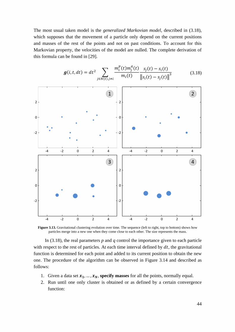
44

The most usual taken model is the generalized Markovian model, described in (3.18),

which supposes that the movement of a particle only depend on the current positions

and masses of the rest of the points and not on past conditions. To account for this

Markovian property, the velocities of the model are nulled. The complete derivation of

this formula can be found in [29].

𝒈(𝑖, 𝑡, 𝑑𝑡) = 𝑑𝑡2 ∑𝑚𝑖𝑝(𝑡)𝑚𝑗

𝑞(𝑡)

𝑚𝑖(𝑡)

𝑠𝑗(𝑡) − 𝑠𝑖(𝑡)

‖𝑠𝑖(𝑡) − 𝑠𝑗(𝑡)‖3

𝑗∈𝑁(𝑡).𝑗≠𝑖

(3.18)

Figure 3.13. Gravitational clustering evolution over time. The sequence (left to right, top to bottom) shows how

particles merge into a new one when they come close to each other. The size represents the mass.

In (3.18), the real parameters p and q control the importance given to each particle

with respect to the rest of particles. At each time interval defined by 𝑑𝑡, the gravitational

function is determined for each point and added to its current position to obtain the new

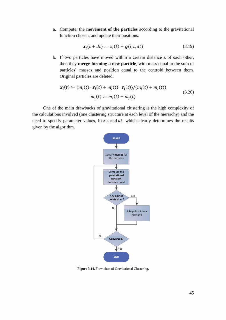
one. The procedure of the algorithm can be observed in Figure 3.14 and described as

follows:

1. Given a data set 𝒙𝟏, … , 𝒙𝑵, specify masses for all the points, normally equal.

2. Run until one only cluster is obtained or as defined by a certain convergence

function:

-2

0

2

0 2 4-2-4

-2

0

2

0 2 4-2-4

-2

0

2

0 2 4-2-4

-2

0

2

0 2 4-2-4

1 2

3 4

45

a. Compute, the movement of the particles according to the gravitational

function chosen, and update their positions.

𝒙𝑖(𝑡 + 𝑑𝑡) ≔ 𝒙𝑖(𝑡) + 𝒈(𝑖, 𝑡, 𝑑𝑡) (3.19)

b. If two particles have moved within a certain distance ε of each other,

then they merge forming a new particle, with mass equal to the sum of

particles’ masses and position equal to the centroid between them.

Original particles are deleted.

𝒙𝒊(𝑡) ≔ (𝑚𝑖(𝑡) · 𝒔𝒊(𝑡) + 𝑚𝑗(𝑡) · 𝒔𝒋(𝑡))/(𝑚𝑖(𝑡) + 𝑚𝑗(𝑡))

𝑚𝑖(𝑡) ≔ 𝑚𝑖(𝑡) + 𝑚𝑗(𝑡) (3.20)

One of the main drawbacks of gravitational clustering is the high complexity of

the calculations involved (one clustering structure at each level of the hierarchy) and the

need to specify parameter values, like ε and 𝑑𝑡, which clearly determines the results

given by the algorithm.

START

Specify masses for the particles

Compute the gravitational

function for each point

Any pair of points at ≤ε?

Join points into a new one

Converged?

END

No

No

Yes

Yes

Figure 3.14. Flow chart of Gravitational Clustering.

46

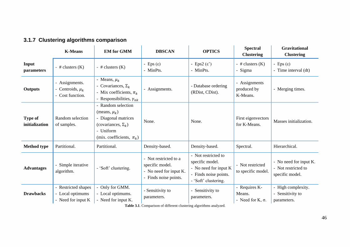
3.1.7 Clustering algorithms comparison

K-Means EM for GMM DBSCAN OPTICS

Spectral

Clustering

Gravitational

Clustering

Input

parameters - # clusters (K) - # clusters (K)

- Eps (ε)

- MinPts.

- Eps2 (ε’)

- MinPts.

- # clusters (K)

- Sigma

- Eps (ε)

- Time interval (dt)

Outputs

- Assignments.

- Centroids, 𝜇𝑘

- Cost function.

- Means, 𝜇𝑘

- Covariances, Σ𝑘

- Mix coefficients, 𝜋𝑘

- Responsibilities, 𝛾𝑛𝑘

- Assignments. - Database ordering

(RDist, CDist).

- Assignments

produced by

K-Means.

- Merging times.

Type of

initialization

Random selection

of samples.

- Random selection

(means, 𝜇𝑘)

- Diagonal matrices

(covariances, Σ𝑘)

- Uniform

(mix. coefficients, 𝜋𝑘)

None. None. First eigenvectors

for K-Means. Masses initialization.

Method type Partitional. Partitional. Density-based. Density-based. Spectral. Hierarchical.

Advantages - Simple iterative

algorithm. - ‘Soft’ clustering.

- Not restricted to a

specific model.

- No need for input K.

- Finds noise points.

- Not restricted to

specific model.

- No need for input K

- Finds noise points.

- ‘Soft’ clustering.

- Not restricted

to specific model.

- No need for input K.

- Not restricted to

specific model.

Drawbacks

- Restricted shapes

- Local optimums

- Need for input K

- Only for GMM.

- Local optimums.

- Need for input K.

- Sensitivity to

parameters.

- Sensitivity to

parameters.

- Requires K-

Means.

- Need for K, σ.

- High complexity.

- Sensitivity to

parameters.

Table 3.1. Comparison of different clustering algorithms analyzed.

47

3.2 Clustering evaluation techniques

Some algorithms, like K-Means or Expectation Maximization, require the number

of clusters to be specified initially. In these cases, since the goal is to identify the cluster

structure, we need to run the same method for each of the possible numbers of clusters

and determine objectively which one fits best the data set.

Also, once the algorithm has correctly detected the modulation format, we would

like to know the percentage of points that have been classified in its optimum cluster, to

discover if the algorithm is reliable and in which grade.

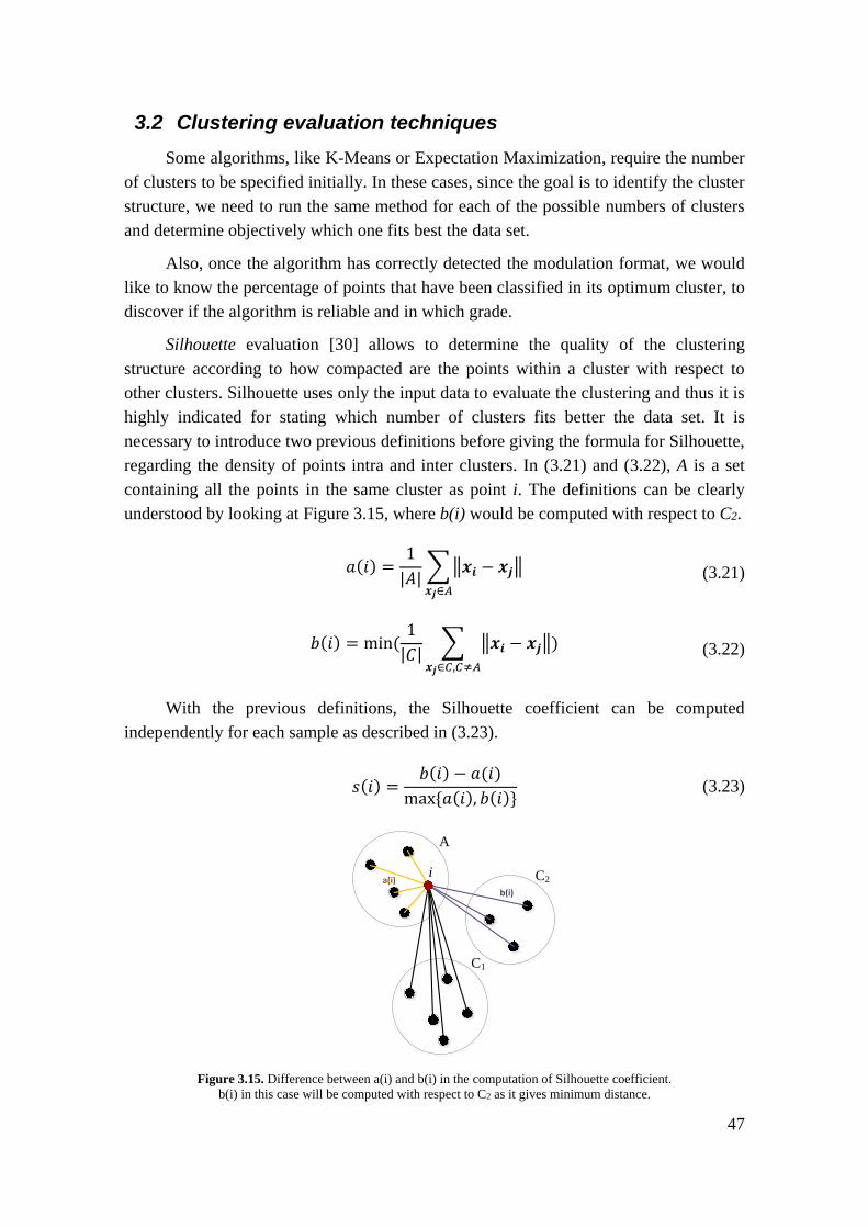
Silhouette evaluation [30] allows to determine the quality of the clustering

structure according to how compacted are the points within a cluster with respect to

other clusters. Silhouette uses only the input data to evaluate the clustering and thus it is

highly indicated for stating which number of clusters fits better the data set. It is

necessary to introduce two previous definitions before giving the formula for Silhouette,

regarding the density of points intra and inter clusters. In (3.21) and (3.22), A is a set

containing all the points in the same cluster as point i. The definitions can be clearly

understood by looking at Figure 3.15, where b(i) would be computed with respect to C2.

𝑎(𝑖) =1

|𝐴|∑‖𝒙𝒊 − 𝒙𝒋‖

𝒙𝒋∈𝐴

(3.21)

𝑏(𝑖) = min (1

|𝐶|∑ ‖𝒙𝒊 − 𝒙𝒋‖

𝒙𝒋∈𝐶,𝐶≠𝐴

) (3.22)

With the previous definitions, the Silhouette coefficient can be computed

independently for each sample as described in (3.23).

𝑠(𝑖) =𝑏(𝑖) − 𝑎(𝑖)

max {𝑎(𝑖), 𝑏(𝑖)} (3.23)

i

A

C1

C2a(i)

b(i)

Figure 3.15. Difference between a(i) and b(i) in the computation of Silhouette coefficient.

b(i) in this case will be computed with respect to C2 as it gives minimum distance.

48

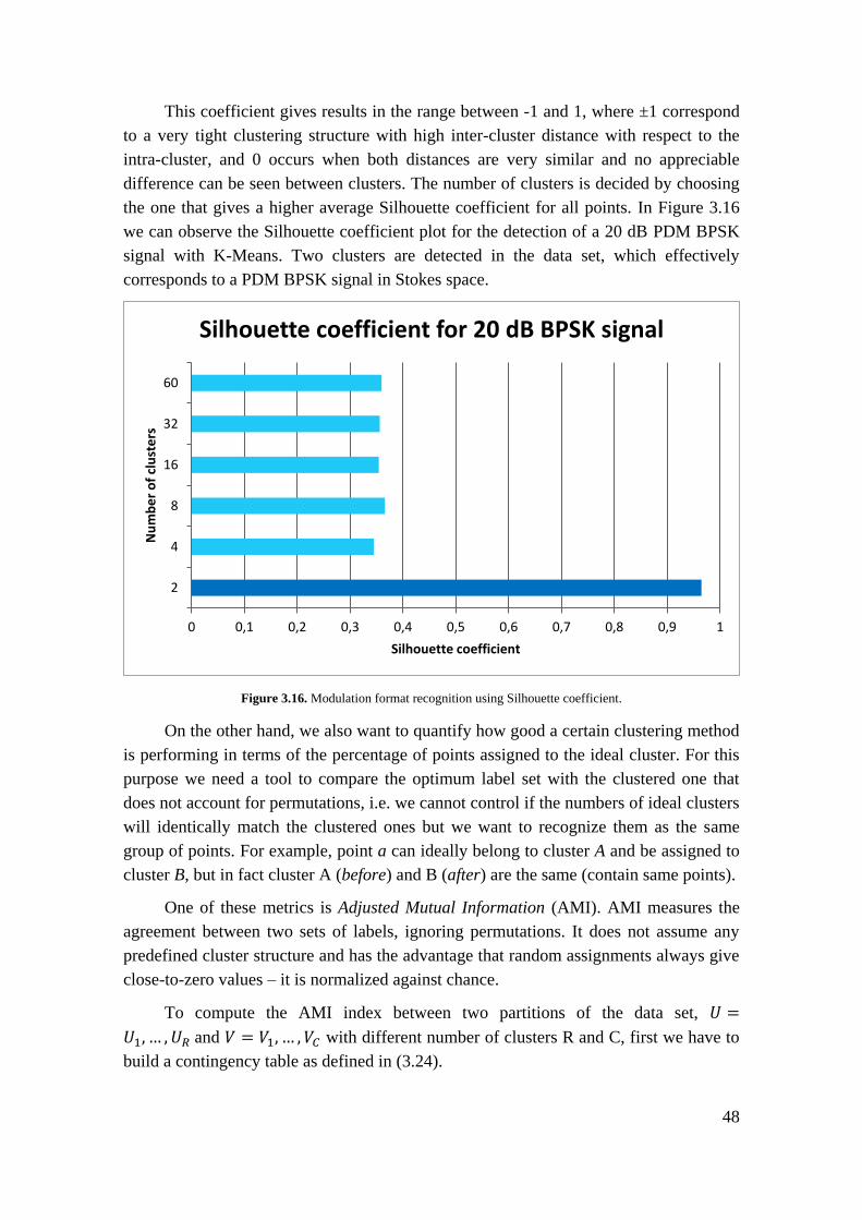
This coefficient gives results in the range between -1 and 1, where ±1 correspond

to a very tight clustering structure with high inter-cluster distance with respect to the

intra-cluster, and 0 occurs when both distances are very similar and no appreciable

difference can be seen between clusters. The number of clusters is decided by choosing

the one that gives a higher average Silhouette coefficient for all points. In Figure 3.16

we can observe the Silhouette coefficient plot for the detection of a 20 dB PDM BPSK

signal with K-Means. Two clusters are detected in the data set, which effectively

corresponds to a PDM BPSK signal in Stokes space.

Figure 3.16. Modulation format recognition using Silhouette coefficient.

On the other hand, we also want to quantify how good a certain clustering method

is performing in terms of the percentage of points assigned to the ideal cluster. For this

purpose we need a tool to compare the optimum label set with the clustered one that

does not account for permutations, i.e. we cannot control if the numbers of ideal clusters

will identically match the clustered ones but we want to recognize them as the same

group of points. For example, point a can ideally belong to cluster A and be assigned to

cluster B, but in fact cluster A (before) and B (after) are the same (contain same points).

One of these metrics is Adjusted Mutual Information (AMI). AMI measures the

agreement between two sets of labels, ignoring permutations. It does not assume any

predefined cluster structure and has the advantage that random assignments always give

close-to-zero values – it is normalized against chance.

To compute the AMI index between two partitions of the data set, 𝑈 =

𝑈1, … , 𝑈𝑅 and 𝑉 = 𝑉1, … , 𝑉𝐶 with different number of clusters R and C, first we have to

build a contingency table as defined in (3.24).

0 0,1 0,2 0,3 0,4 0,5 0,6 0,7 0,8 0,9 1

2

4

8

16

32

60

Silhouette coefficient

Nu

mb

er

of

clu

ste

rs

Silhouette coefficient for 20 dB BPSK signal

49

𝑚𝑖𝑗 = |𝑈𝑖 ∩ 𝑉𝑗| ∀𝑖 = 1: 𝑅, ∀𝑗 = 1: 𝐶 (3.24)

From information theory, the mutual information between two random variables

can be defined as in (3.25) with 𝑝(𝑖) being the probability that an object is assigned into

𝑈𝑖 and 𝑝(𝑖, 𝑗) the probability that an object belongs to both 𝑈𝑖 and 𝑉𝑗.

𝑀𝐼(𝑈, 𝑉) =∑∑𝑝(𝑖, 𝑗) · log (𝑝(𝑖, 𝑗)

𝑝(𝑖)𝑝(𝑗))

|𝑉|

𝑗=1

|𝑈|

𝑖=1

(3.25)

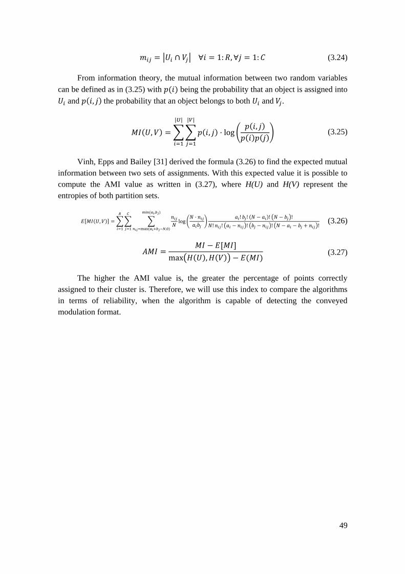
Vinh, Epps and Bailey [31] derived the formula (3.26) to find the expected mutual

information between two sets of assignments. With this expected value it is possible to

compute the AMI value as written in (3.27), where H(U) and H(V) represent the

entropies of both partition sets.

𝐸[𝑀𝐼(𝑈, 𝑉)] =∑∑ ∑𝑛𝑖𝑗

𝑁log (

𝑁 · 𝑛𝑖𝑗

𝑎𝑖𝑏𝑗)

𝑎𝑖! 𝑏𝑗! (𝑁 − 𝑎𝑖)! (𝑁 − 𝑏𝑗)!

𝑁! 𝑛𝑖𝑗! (𝑎𝑖 − 𝑛𝑖𝑗)! (𝑏𝑗 − 𝑛𝑖𝑗)! (𝑁 − 𝑎𝑖 − 𝑏𝑗 + 𝑛𝑖𝑗)!

min (𝑎𝑖,𝑏𝑗)

𝑛𝑖𝑗=max (𝑎𝑖+𝑏𝑗−𝑁,0)

𝐶

𝑗=1

𝑅

𝑖=1

(3.26)

𝐴𝑀𝐼 =𝑀𝐼 − 𝐸[𝑀𝐼]

max(𝐻(𝑈), 𝐻(𝑉)) − 𝐸(𝑀𝐼) (3.27)

The higher the AMI value is, the greater the percentage of points correctly

assigned to their cluster is. Therefore, we will use this index to compare the algorithms

in terms of reliability, when the algorithm is capable of detecting the conveyed

modulation format.

50

51

4 Proposed algorithm for modulation format recognition based on Maximum Likelihood in Stokes space

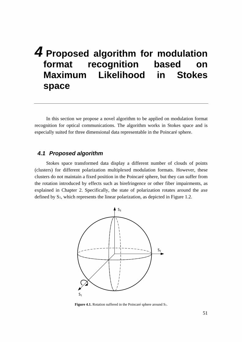
In this section we propose a novel algorithm to be applied on modulation format

recognition for optical communications. The algorithm works in Stokes space and is

especially suited for three dimensional data representable in the Poincaré sphere.

4.1 Proposed algorithm

Stokes space transformed data display a different number of clouds of points

(clusters) for different polarization multiplexed modulation formats. However, these

clusters do not maintain a fixed position in the Poincaré sphere, but they can suffer from

the rotation introduced by effects such as birefringence or other fiber impairments, as

explained in Chapter 2. Specifically, the state of polarization rotates around the axe

defined by S1, which represents the linear polarization, as depicted in Figure 1.2.

S1

S3

S2

Figure 4.1. Rotation suffered in the Poincaré sphere around S1.

52

If we could determine the angle of rotation the received signal has with respect to

a certain initial position of the centroids, then we would be able to identify the

transmission parameters by comparing the incoming signal with the stored centroids

positions rotated by the optimum angle computed. This is essentially what the proposed

algorithm does.

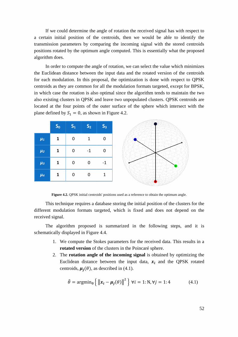
In order to compute the angle of rotation, we can select the value which minimizes

the Euclidean distance between the input data and the rotated version of the centroids

for each modulation. In this proposal, the optimization is done with respect to QPSK

centroids as they are common for all the modulation formats targeted, except for BPSK,

in which case the rotation is also optimal since the algorithm tends to maintain the two

also existing clusters in QPSK and leave two unpopulated clusters. QPSK centroids are

located at the four points of the outer surface of the sphere which intersect with the

plane defined by 𝑆1 = 0, as shown in Figure 4.2.

S0 S1 S2 S3

µ1 1 0 1 0

µ2 1 0 -1 0

µ3 1 0 0 -1

µ4 1 0 0 1

Figure 4.2. QPSK initial centroids' positions used as a reference to obtain the optimum angle.

This technique requires a database storing the initial position of the clusters for the

different modulation formats targeted, which is fixed and does not depend on the

received signal.

The algorithm proposed is summarized in the following steps, and it is

schematically displayed in Figure 4.4.

1. We compute the Stokes parameters for the received data. This results in a

rotated version of the clusters in the Poincaré sphere.

2. The rotation angle of the incoming signal is obtained by optimizing the

Euclidean distance between the input data, 𝒙𝒊 and the QPSK rotated

centroids, 𝝁𝒋(𝜃), as described in (4.1).

𝜃 = argminθ { ‖𝒙𝒊 − 𝝁𝒋(𝜃)‖2 } ∀𝑖 = 1: N, ∀𝑗 = 1: 4 (4.1)

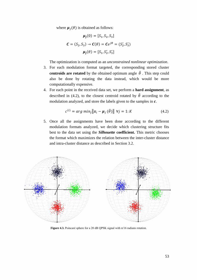
53

where 𝝁𝑗(𝜃) is obtained as follows:

𝝁𝒋(0) = [𝑆1, 𝑆2, 𝑆3]

𝑪 = (𝑆2, 𝑆3) → 𝑪(𝜃) = 𝑪𝑒𝑗𝜃 = (𝑆2

′ , 𝑆3′)

𝝁𝒋(𝜃) = [𝑆1, 𝑆2′ , 𝑆3

′ ]

The optimization is computed as an unconstrained nonlinear optimization.

3. For each modulation format targeted, the corresponding stored cluster

centroids are rotated by the obtained optimum angle 𝜃 . This step could

also be done by rotating the data instead, which would be more

computationally expensive.

4. For each point in the received data set, we perform a hard assignment, as

described in (4.2), to the closest centroid rotated by 𝜃 according to the

modulation analyzed, and store the labels given to the samples in 𝒄.

𝑐(𝑖) = 𝑎𝑟𝑔 𝑚𝑖𝑛𝑗‖𝒙𝑖 − 𝝁𝑗 (𝜃)‖ ∀𝑗 = 1:𝐾 (4.2)

5. Once all the assignments have been done according to the different

modulation formats analyzed, we decide which clustering structure fits

best to the data set using the Silhouette coefficient. This metric chooses

the format which maximizes the relation between the inter-cluster distance

and intra-cluster distance as described in Section 3.2.

Figure 4.3. Poincaré sphere for a 20 dB QPSK signal with π/16 radians rotation.

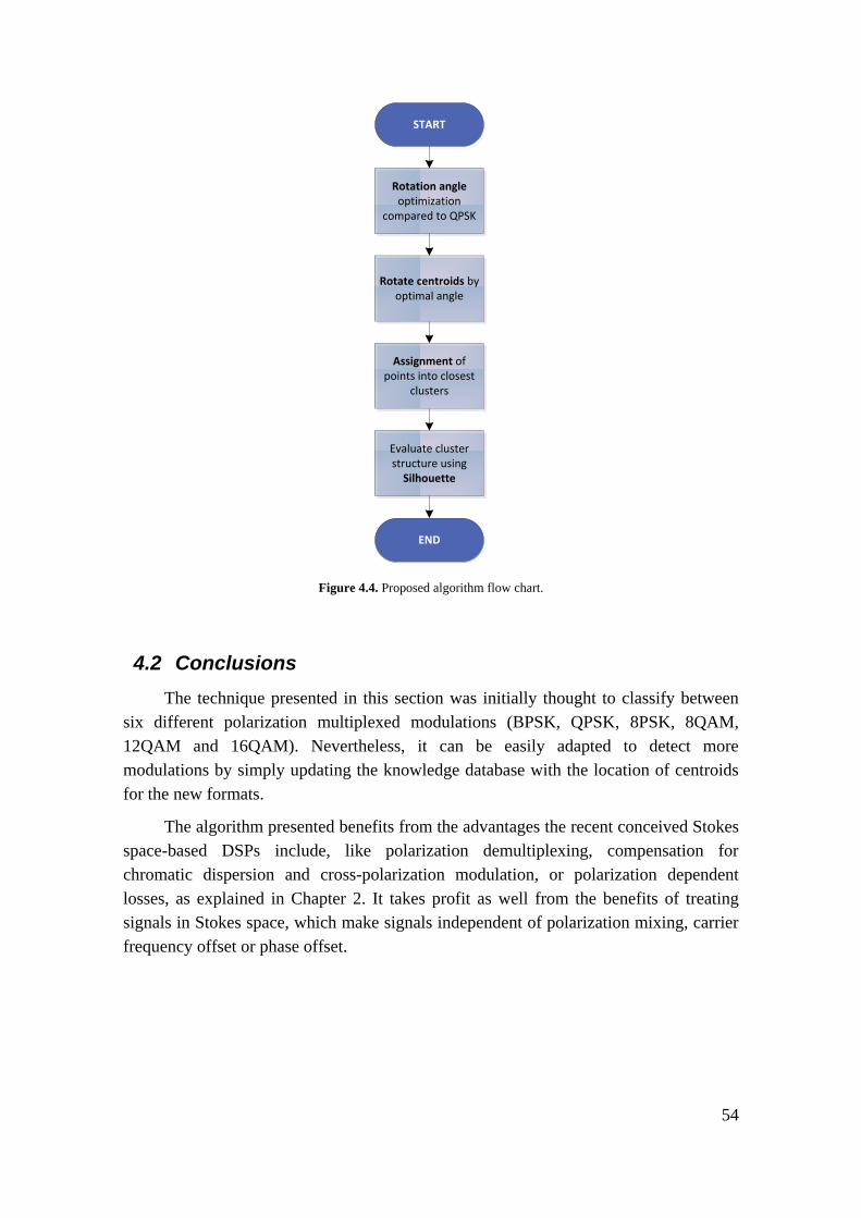
54

START

Rotation angle optimization

compared to QPSK

Rotate centroids by optimal angle

Assignment of points into closest

clusters

Evaluate cluster structure using

Silhouette

END

Figure 4.4. Proposed algorithm flow chart.

4.2 Conclusions

The technique presented in this section was initially thought to classify between

six different polarization multiplexed modulations (BPSK, QPSK, 8PSK, 8QAM,

12QAM and 16QAM). Nevertheless, it can be easily adapted to detect more

modulations by simply updating the knowledge database with the location of centroids

for the new formats.

The algorithm presented benefits from the advantages the recent conceived Stokes

space-based DSPs include, like polarization demultiplexing, compensation for

chromatic dispersion and cross-polarization modulation, or polarization dependent

losses, as explained in Chapter 2. It takes profit as well from the benefits of treating

signals in Stokes space, which make signals independent of polarization mixing, carrier

frequency offset or phase offset.

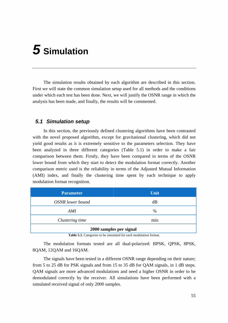
55

5 Simulation

The simulation results obtained by each algorithm are described in this section.

First we will state the common simulation setup used for all methods and the conditions

under which each test has been done. Next, we will justify the OSNR range in which the

analysis has been made, and finally, the results will be commented.

5.1 Simulation setup

In this section, the previously defined clustering algorithms have been contrasted

with the novel proposed algorithm, except for gravitational clustering, which did not

yield good results as it is extremely sensitive to the parameters selection. They have

been analyzed in three different categories (Table 5.1) in order to make a fair

comparison between them. Firstly, they have been compared in terms of the OSNR

lower bound from which they start to detect the modulation format correctly. Another

comparison metric used is the reliability in terms of the Adjusted Mutual Information

(AMI) index, and finally the clustering time spent by each technique to apply

modulation format recognition.

Parameter Unit

OSNR lower bound dB

AMI %

Clustering time min

2000 samples per signal

Table 5.1. Categories to be simulated for each modulation format.

The modulation formats tested are all dual-polarized: BPSK, QPSK, 8PSK,

8QAM, 12QAM and 16QAM.

The signals have been tested in a different OSNR range depending on their nature;

from 5 to 25 dB for PSK signals and from 15 to 35 dB for QAM signals, in 1 dB steps.

QAM signals are more advanced modulations and need a higher OSNR in order to be

demodulated correctly by the receiver. All simulations have been performed with a

simulated received signal of only 2000 samples.

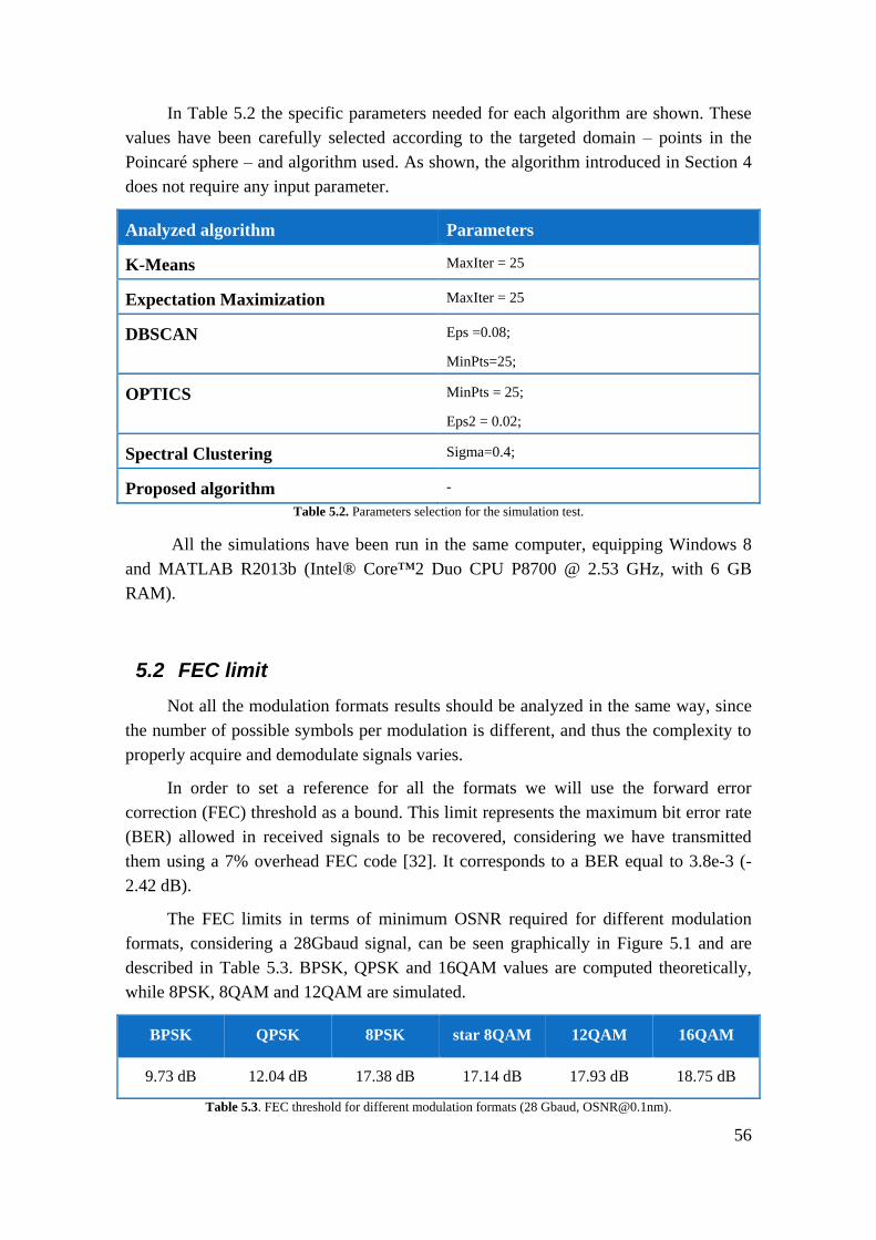
56

In Table 5.2 the specific parameters needed for each algorithm are shown. These

values have been carefully selected according to the targeted domain – points in the

Poincaré sphere – and algorithm used. As shown, the algorithm introduced in Section 4

does not require any input parameter.

Analyzed algorithm Parameters

K-Means MaxIter = 25

Expectation Maximization MaxIter = 25

DBSCAN Eps =0.08;

MinPts=25;

OPTICS MinPts = 25;

Eps2 = 0.02;

Spectral Clustering Sigma=0.4;

Proposed algorithm -

Table 5.2. Parameters selection for the simulation test.

All the simulations have been run in the same computer, equipping Windows 8

and MATLAB R2013b (Intel® Core™2 Duo CPU P8700 @ 2.53 GHz, with 6 GB

RAM).

5.2 FEC limit

Not all the modulation formats results should be analyzed in the same way, since

the number of possible symbols per modulation is different, and thus the complexity to

properly acquire and demodulate signals varies.

In order to set a reference for all the formats we will use the forward error

correction (FEC) threshold as a bound. This limit represents the maximum bit error rate

(BER) allowed in received signals to be recovered, considering we have transmitted

them using a 7% overhead FEC code [32]. It corresponds to a BER equal to 3.8e-3 (-

2.42 dB).

The FEC limits in terms of minimum OSNR required for different modulation

formats, considering a 28Gbaud signal, can be seen graphically in Figure 5.1 and are

described in Table 5.3. BPSK, QPSK and 16QAM values are computed theoretically,

while 8PSK, 8QAM and 12QAM are simulated.

BPSK QPSK 8PSK star 8QAM 12QAM 16QAM

9.73 dB 12.04 dB 17.38 dB 17.14 dB 17.93 dB 18.75 dB

Table 5.3. FEC threshold for different modulation formats (28 Gbaud, OSNR@0.1nm).

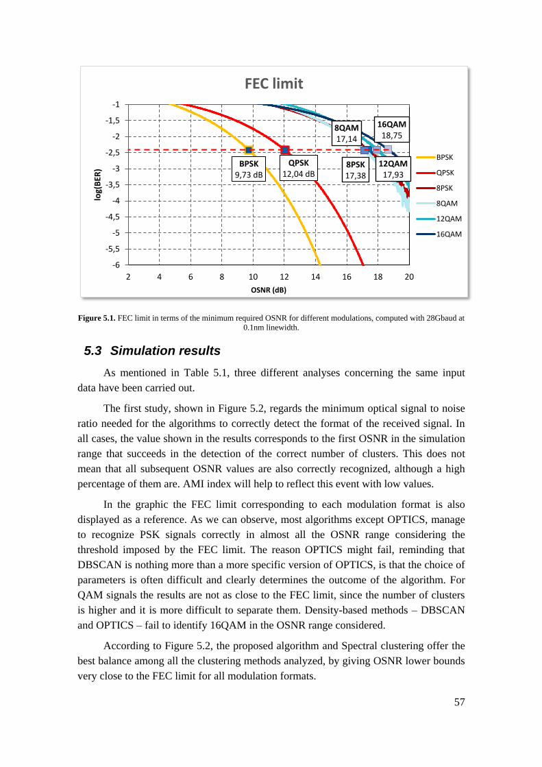
57

Figure 5.1. FEC limit in terms of the minimum required OSNR for different modulations, computed with 28Gbaud at

0.1nm linewidth.

5.3 Simulation results

As mentioned in Table 5.1, three different analyses concerning the same input

data have been carried out.

The first study, shown in Figure 5.2, regards the minimum optical signal to noise

ratio needed for the algorithms to correctly detect the format of the received signal. In

all cases, the value shown in the results corresponds to the first OSNR in the simulation

range that succeeds in the detection of the correct number of clusters. This does not

mean that all subsequent OSNR values are also correctly recognized, although a high

percentage of them are. AMI index will help to reflect this event with low values.

In the graphic the FEC limit corresponding to each modulation format is also

displayed as a reference. As we can observe, most algorithms except OPTICS, manage

to recognize PSK signals correctly in almost all the OSNR range considering the

threshold imposed by the FEC limit. The reason OPTICS might fail, reminding that

DBSCAN is nothing more than a more specific version of OPTICS, is that the choice of

parameters is often difficult and clearly determines the outcome of the algorithm. For

QAM signals the results are not as close to the FEC limit, since the number of clusters

is higher and it is more difficult to separate them. Density-based methods – DBSCAN

and OPTICS – fail to identify 16QAM in the OSNR range considered.

According to Figure 5.2, the proposed algorithm and Spectral clustering offer the

best balance among all the clustering methods analyzed, by giving OSNR lower bounds

very close to the FEC limit for all modulation formats.

BPSK9,73 dB

QPSK12,04 dB

8PSK17,38

8QAM17,14

12QAM17,93

16QAM18,75

-6

-5,5

-5

-4,5

-4

-3,5

-3

-2,5

-2

-1,5

-1

2 4 6 8 10 12 14 16 18 20

log(

BER

)

OSNR (dB)

FEC limit

BPSK

QPSK

8PSK

8QAM

12QAM

16QAM

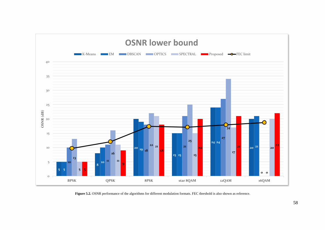
58

Figure 5.2. OSNR performance of the algorithms for different modulation formats. FEC threshold is also shown as reference.

58

20

15

24

20

5

10

19

15

2421

10 11

1821

27

0

1316

2225

34

05

11

21

1517

20

5

9

1820 21 22

0

5

10

15

20

25

30

35

40

BPSK QPSK 8PSK star 8QAM 12QAM 16QAM

OS

NR

(d

B)

OSNR lower boundK-Means EM DBSCAN OPTICS SPECTRAL Proposed FEC limit

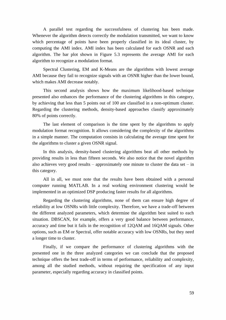
59

A parallel test regarding the successfulness of clustering has been made.

Whenever the algorithm detects correctly the modulation transmitted, we want to know

which percentage of points have been properly classified in its ideal cluster, by

computing the AMI index. AMI index has been calculated for each OSNR and each

algorithm. The bar plot shown in Figure 5.3 represents the average AMI for each

algorithm to recognize a modulation format.

Spectral Clustering, EM and K-Means are the algorithms with lowest average

AMI because they fail to recognize signals with an OSNR higher than the lower bound,

which makes AMI decrease notably.

This second analysis shows how the maximum likelihood-based technique

presented also enhances the performance of the clustering algorithms in this category,

by achieving that less than 5 points out of 100 are classified in a non-optimum cluster.

Regarding the clustering methods, density-based approaches classify approximately

80% of points correctly.

The last element of comparison is the time spent by the algorithms to apply

modulation format recognition. It allows considering the complexity of the algorithms

in a simple manner. The computation consists in calculating the average time spent for

the algorithms to cluster a given OSNR signal.

In this analysis, density-based clustering algorithms beat all other methods by

providing results in less than fifteen seconds. We also notice that the novel algorithm

also achieves very good results – approximately one minute to cluster the data set – in

this category.

All in all, we must note that the results have been obtained with a personal

computer running MATLAB. In a real working environment clustering would be

implemented in an optimized DSP producing faster results for all algorithms.

Regarding the clustering algorithms, none of them can ensure high degree of

reliability at low OSNRs with little complexity. Therefore, we have a trade-off between

the different analyzed parameters, which determine the algorithm best suited to each

situation. DBSCAN, for example, offers a very good balance between performance,

accuracy and time but it fails in the recognition of 12QAM and 16QAM signals. Other

options, such as EM or Spectral, offer notable accuracy with low OSNRs, but they need

a longer time to cluster.

Finally, if we compare the performance of clustering algorithms with the

presented one in the three analyzed categories we can conclude that the proposed

technique offers the best trade-off in terms of performance, reliability and complexity,

among all the studied methods, without requiring the specification of any input

parameter, especially regarding accuracy in classified points.

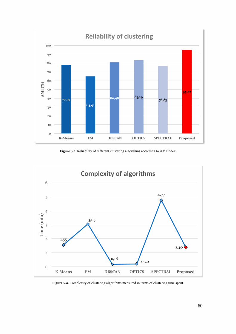
60

Figure 5.3. Reliability of different clustering algorithms according to AMI index.

Figure 5.4. Complexity of clustering algorithms measured in terms of clustering time spent.

77,92

64,91

80,98 83,2976,83

95,07

0

10

20

30

40

50

60

70

80

90

100

K-Means EM DBSCAN OPTICS SPECTRAL Proposed

AM

I (%

)Reliability of clustering

1,55

3,05

0,180,20

4,77

1,40

0

1

2

3

4

5

6

K-Means EM DBSCAN OPTICS SPECTRAL Proposed

Tim

e (

min

)

Complexity of algorithms

61

6 Conclusions

Optical networks are envisaged to become cognitive in the next few years in order

to tackle the unceasing increase in Internet applications and users, and their

corresponding different quality of service parameters. Cognition involves all the

activities leading to an optimization of the whole network performance by acting and

learning according to the current and past observations of the link conditions.

One of the fundamental functionalities implemented in cognitive networks is

modulation format recognition, which makes possible to use a single universal receiver

capable of autonomously detecting the modulation format of the received signal without

any prior information. In the state-of-the-art we have examined the different alternatives

analyzed up to now, specially focusing in the stage of the DSP they apply.

In this thesis the approach followed to identify the modulation has been to use the

Stokes space representation of the signals, providing the beneficial features introduced

in Stokes space-based DSPs lately and the advantages of this mapping. After studying

the main aspects about polarization demultiplexing, necessary to understand the nature

of the signals targeted in this thesis, we have conducted an intensive research on six

different clustering algorithms (K-Means, Expectation Maximization, DBSCAN,

OPTICS, Spectral clustering and Gravitational clustering).

To our knowledge, it is the first time different clustering algorithms are compared

in the same study for modulation format recognition in fiber-optic communications,

targeting six possible modulation formats (PDM BPSK, PDM QPSK, PDM 8PSK,

PDM 8QAM, PDM 16QAM and PDM 32QAM).

Moreover, we have proposed a novel algorithm to be applied for modulation

format identification in Stokes space, based on maximum likelihood between the

received signal and the possible modulation formats configurations. It offers the

advantages of dealing with signals in Stokes space and, in addition, benefits from the

specific knowledge of each modulation format treated.

The different algorithms have been compared in three categories – OSNR

performance, reliability (AMI) and complexity (clustering time) – to evaluate their

expected performance in a real environment and assess their feasibility. The results

obtained confirm the proposed algorithm as a very suitable solution for modulation

format recognition in fiber-optic communications since it yields an almost optimal

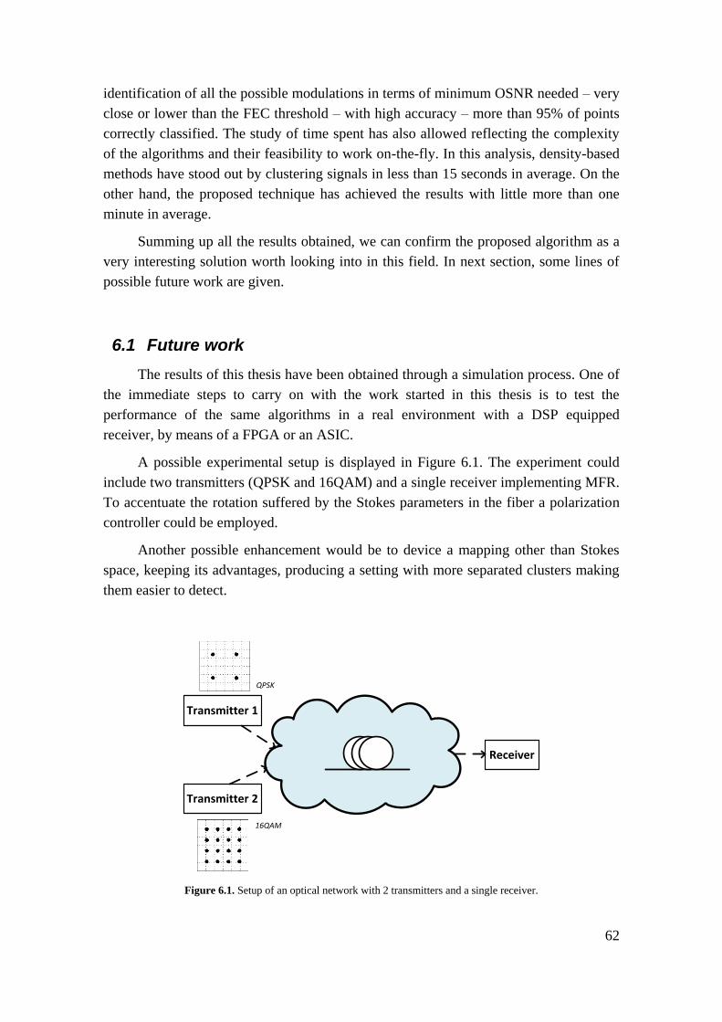
62

identification of all the possible modulations in terms of minimum OSNR needed – very

close or lower than the FEC threshold – with high accuracy – more than 95% of points

correctly classified. The study of time spent has also allowed reflecting the complexity

of the algorithms and their feasibility to work on-the-fly. In this analysis, density-based

methods have stood out by clustering signals in less than 15 seconds in average. On the

other hand, the proposed technique has achieved the results with little more than one

minute in average.

Summing up all the results obtained, we can confirm the proposed algorithm as a

very interesting solution worth looking into in this field. In next section, some lines of

possible future work are given.

6.1 Future work

The results of this thesis have been obtained through a simulation process. One of

the immediate steps to carry on with the work started in this thesis is to test the

performance of the same algorithms in a real environment with a DSP equipped

receiver, by means of a FPGA or an ASIC.

A possible experimental setup is displayed in Figure 6.1. The experiment could

include two transmitters (QPSK and 16QAM) and a single receiver implementing MFR.

To accentuate the rotation suffered by the Stokes parameters in the fiber a polarization

controller could be employed.

Another possible enhancement would be to device a mapping other than Stokes

space, keeping its advantages, producing a setting with more separated clusters making

them easier to detect.

Transmitter 1

Receiver

Transmitter 2

QPSK

16QAM

Figure 6.1. Setup of an optical network with 2 transmitters and a single receiver.

63

7 References

[1] Cisco Systems, “Cisco Visual Networking Index : Forecast and Methodology , 2012 – 2017,” pp.

1–15, 2013.

[2] R. W. Thomas, D. H. Friend, L. A. Dasilva, and B. Allen, “Cognitive Networks,” in Cognitive

Radio, Software Defined Radio, and Adaptive Wireless Systems, vol. 44, 2007, pp. 17–41.

[3] Z. Wang, H. Wang, G. Feng, B. Li, and X. Chen, “Cognitive Networks and Its Layered Cognitive

Architecture,” 2010 Fifth Int. Conf. Internet Comput. Sci. Eng., pp. 145–148, 2010.

[4] R. Borkowski, “Enabling Technologies for Cognitive Optical Networks.” PhD Thesis, DTU

Fotonik, 2014.

[5] I. de Miguel, R. J. Durán, T. Jiménez, N. Fernández, J. C. Aguado, R. M. Lorenzo, A. Caballero,

I. Tafur Monroy, Y. Ye, A. Tymecki, I. Tomkos, M. Angelou, D. Klonidis, A. Francescon, D.

Siracusa, and E. Salvadori, “Cognitive dynamic optical networks [Invited],” J. Opt. Commun.

Netw., vol. 5, pp. A107–A118, 2013.

[6] G. S. Zervas and D. Simeonidou, “Cognitive optical networks: Need, requirements and

architecture,” Transparent Opt. Networks (ICTON), 2010 12th Int. Conf., 2010.

[7] W. Wei, C. Wang, and J. Yu, “Cognitive optical networks: Key drivers, enabling techniques, and

adaptive bandwidth services,” in IEEE Communications Magazine, 2012, vol. 50, pp. 106–113.

[8] CHRON, “The CHRON Project.” [Online]. Available: http://www.ict-chron.eu.

[9] O. A. Dobre, A. Abdi, and W. Su, “Survey of automatic modulation classification techniques :

classical approaches and new trends,” pp. 137–156.

[10] J. Mitola, “Cognitive Radio: An Integrated Agent Architecture for Software Defined Radio,”

2000.

[11] C. Ramming, “Cognitive Networks,” in DARPATech Symposium. Anaheim, CA, USA, 2004.

[12] N. G. Gonzalez, D. Zibar, and I. T. Monroy, “Cognitive digital receiver for burst mode phase

modulated radio over fiber links,” Opt. Commun. (ECOC), 2010 36th Eur. Conf. Exhib., 2010.

[13] F. N. Khan, Y. Zhou, A. P. T. Lau, and C. Lu, “Modulation format identification in

heterogeneous fiber-optic networks using artificial neural networks.,” Opt. Express, vol. 20, no.

11, pp. 12422–31, May 2012.

[14] P. Isautier, A. Stark, K. Mehta, R. de Salvo, and S. E. Ralph, “Autonomous Software-Defined

Coherent Optical Receivers,” in Optical Fiber Communication Conference/National Fiber Optic

Engineers Conference 2013, 2013, p. OTh3B.4.

64

[15] R. Borkowski, D. Zibar, A. Caballero, V. Arlunno, and I. T. Monroy, “Stokes Space-Based

Optical Modulation Format Recognition for Digital Coherent Receivers,” IEEE Photonics

Technol. Lett., vol. 25, no. 21, pp. 2129–2132, Nov. 2013.

[16] J. Liu, Z. Dong, K. P. Zhong, A. P. T. Lau, C. Lu, and Y. Lu, “Modulation Format Identification

Based on Received Signal Power Distributions for Digital Coherent Receivers,” in Optical Fiber

Communication Conference, 2014, p. Th4D.3.

[17] E. J. Adles, M. L. Dennis, S. Member, W. R. Johnson, T. P. Mckenna, C. R. Menyuk, J. E. Sluz,

R. M. Sova, M. G. Taylor, and R. A. Venkat, “Blind Optical Modulation Format Identification

From Physical Layer Characteristics,” J. Light. Technol., vol. 32, no. 8, pp. 1501–1509, 2014.

[18] A. Kumar and A. Ghatak, Polarization of Light with Applications in Optical Fibers, Illustrate.

SPIE Press, 2011, pp. 75–135.

[19] B. Szafraniec, B. Nebendahl, and T. Marshall, “Polarization demultiplexing in Stokes space.,”

Opt. Express, vol. 18, no. 17, pp. 17928–39, Aug. 2010.

[20] C. M. Bishop, “Pattern Recognition and Machine Learning (Information Science and Statistics),”

Aug. 2006.

[21] A. K. Jain, M. N. Murty, and P. J. Flynn, “Data clustering: a review,” ACM Computing Surveys,

vol. 31, no. 3. pp. 264–323, 1999.

[22] J. Macqueen, “Some methods for classification and analysis of multivariate observations,” Proc.

Fifth Berkeley Symp. Math. Stat. Probab., vol. 1, pp. 281–297, 1967.

[23] A. P. Dempster, N. M. Laird, and D. B. Rubin, “Maximum Likelihood from Incomplete Data via

the EM Algorithm,” J. R. Stat. Soc. Ser. B, vol. 39, pp. 1–38, 1977.

[24] C. M. Bishop, Pattern Recognition and Machine Learning, vol. 4. Springer-Verlag New York,

Inc., 2006, pp. 1–738.

[25] M. Ester, H. P. Kriegel, J. Sander, and X. Xu, “A Density-Based Algorithm for Discovering

Clusters in Large Spatial Databases with Noise,” in Second International Conference on

Knowledge Discovery and Data Mining, 1996, pp. 226–231.

[26] M. Ankerst, M. M. Breunig, H.-P. Kriegel, and J. Sander, “OPTICS: ordering points to identify

the clustering structure,” ACM SIGMOD Rec., vol. 28, pp. 49–60, 1999.

[27] U. Luxburg, “A tutorial on spectral clustering,” Stat. Comput., vol. 17, no. 4, pp. 395–416, Aug.

2007.

[28] A. Y. Ng, M. I. Jordan, and Y. Weiss, “On spectral clustering: Analysis and an algorithm,” in

Advances in Neural Information Processing Systems, 2001, pp. 849–856.

[29] W. E. Wright, “Gravitational clustering,” Pattern Recognition, vol. 9, no. 3. pp. 151–166, 1977.

[30] P. J. Rousseeuw, “Silhouettes: A graphical aid to the interpretation and validation of cluster

analysis,” Journal of Computational and Applied Mathematics, vol. 20. pp. 53–65, 1987.

[31] N. X. Vinh, “Information Theoretic Measures for Clusterings Comparison : Variants , Properties ,

Normalization and Correction for Chance,” J. Mach. Learn. Res., vol. 11, pp. 2837–2854, 2010.

[32] I.-T. S. Group, “ITU-T Rec. G.975.1 (02/2004) Forward error correction for high bit-rate DWDM

submarine systems,” Standard, pp. 1–58, 2005.