Low Cost, Compact Microwave Reflectometer for Non-Destructive Testing
Matthew Rangen and Keith Bruno
March 3, 2005
Bradley University
Department of Electrical and Computer Engineering

Overview
• Objective
• Background
• Block Diagram
• Tasks & Schedule
• Current Results• MATLAB• Network Analyzer
• Future Work

Objective
The objective of the project is to determine the reflection coefficient of an unknown load by the use of a six-port network analyzer integrated with a workstation.

Background
The reflection coefficient can be found by knowing a reference signal and sampling selected power outputs in a micro-strip circuit. With these known quantities and using a specific algorithm, the reflection coefficient can be calculated.

Detailed Block Diagram
Tasks & Schedule(previous)
Final Exams6 to11May
Final Report due, Presentation & Final Exams29 to 5April/May
Final Report & Presentation Preparation22 to 28
Verify Operation15 to 21
·8 to 14
System Integration & Testing1 to 7April
··25 to 31
Test 6-Port·18 to 24
Spring Break11 to 17
·Test Programming Code4 to 10March
Fabricate 6-PortIntegrate MATLAB & A/D25 to 3Feb/March
Design & Simulate InterfaceTest Equations18 to 24
·Implement Equations in MATLAB11 to 17
Design & Simulate 6-Port ·4 to 10February
Purchase: Detectors & USB A/D
Simulate & Test 90º Hybrid ·28 to 3Jan/Feb
Design 90º HybridDevelop Calibration& Measuring Equations
21 to 27January
Keith BrunoMatthew Rangen

MATLAB Work
OverallCalibrationFlowchart

Calibration Work
Calibration FlowEquations
€
pi, k = Pi , k /P 4, k
TS , R = pi , k / pi , 5
Γk /Γk
2= ck + jsk
γi = (cj − ck)[(si − sj)(ck − cl) − (ci − cj)(sk − sl)] + (ck − cl)[(sl − si)(cj − ck) − (cl − ci)(sj − sk)]
fn = Tn, k *k=1
4
∑ γk
gn = Tn, k *k=1
4
∑ γk *ck
hn = 2 * Tn, k *k=1
4
∑ γ * sk
en =
(Tn, k −1) *k=1
4
∑ γk
Γk
2

Calibration Work
Calibration Flow Equations Part 2
€
ξ 1 = (gs * hd) − (hs * gd)
ξ 2 = (hs * fd) − ( fs * hd)
ξ 3 = (hs *ed) − (es * hd)
ξ 4 = (gs * fd) − ( fs * gd)
ξ 5 = (gs *ed) − (es * gd)
Mi , j =(ξ 1
2 /2) −ξ 2ξ 3 −ξ 4ξ 5
ξ 22 + ξ 4
2
Ni , j =ξ 3
2 + ξ 52
ξ 22 + ξ 4
2
A4
2= Mi , j − (Mi , j
2 −Ni , j)(1/ 2)
a4 =A4
2*ξ 2 + ξ 3
ξ 1
b4 =A4
2*ξ 4 + ξ 5
ξ 1

Calibration Work
Calibration Flow Equations Part 3
€
Ri , k =Ti , k −1
Γk
2 + Ti , k[ A4
2+ 2 *ck * a4 − 2* sk *b4]
ai =Ri , l(sm − sn) + Ri , m(sn − sl) + Ri , n(sl − sm)
2[cl(sm − sn) + cm(sn − sl) + cn(sl − sm)
bi =Ri , l(cm − cn) + Ri , m(cn − cl) + Ri , n(cl − cm)
2[cl(sm − sn) + cm(sn − sl) + cn(sl − sm)
Ai = ai + jbi

MATLAB Work
MeasureFlowchart

Measurement Work
Measurement Equations
€
Ai = ai + jbi
Fi =(−1)i
2qi[ Aj
2(bk −bl) + Ak
2(bl −bj) + Al
2(bj −bk)]
Gi =(−1)i
2qi[ Aj
2(ak − al) + Ak
2(al − aj) + Al
2(aj − ak)]
Hi =(−1)i
2qi[ Aj
2(akbl − albk) + Ak
2(albj − ajbl) + Al
2(ajbk − akbj)]
Γt =
Fi *Pi , t + ji=1
4
∑ Gi *Pi , t
i=1
4
∑
Hi *Pi , t
i=1
4
∑

6-Port Network Analyzer
MSUBMSub1
Rough=0.0948 milTanD=0.0013T=1.4 milHu=3.9e+34 milCond=5.8E+7Mur=1Er=3.0H=20.0 mil
MSub
S_ParamSP1
Step=1.0 MHzStop=8.0 GHzStart=4.0 GHz
S-PARAMETERS
V_1ToneSRC1
Freq=6 GHzV=polar(1,0) V
RR1R=50 Ohm
TermTerm4
Z=50 OhmNum=4
TermTerm5
Z=50 OhmNum=5
TermTerm3
Z=50 OhmNum=3
TermTerm6
Z=50 OhmNum=6
MLANGLang1
L=9.04 mmS=5.1 milW=3.8 milSubst="MSub1"
Hybrid90HYB3
PhaseBal=0GainBal=0 dBLoss=0 dB
-900
IN ISO
Hybrid90HYB2
PhaseBal=0GainBal=0 dBLoss=0 dB
-900
IN ISO
Hybrid90HYB4
PhaseBal=0GainBal=0 dBLoss=0 dB
-900
IN ISO
TermTerm2
Z=50 OhmNum=2
TermTerm1
Z=50 OhmNum=1
Hybrid90HYB1
PhaseBal=0GainBal=0 dBLoss=0 dB
-900
IN ISO

90° Hybrid
Input Port Output Port
Isolated Port Output Port
}90° phase-shift
difference

90° Hybrid
TermTerm3
Z=50 OhmNum=3
MLINTL16
L=3.2029 cmW=0.127701 cmSubst="MSub1"
MLINTL15
L=3.2029 cmW=0.127701 cmSubst="MSub1"
TermTerm4
Z=50 OhmNum=4
S_ParamSP1
Step=1.0 MHzStop=8.0 GHzStart=4.0 GHz
S-PARAMETERS
MSUBMSub1
Rough=0.0948 milTanD=0.0013T=1.4 milHu=3.9e+34 milCond=5.8E+7Mur=1Er=3.0H=20.0 mil
MSub
MLINTL14
L=3.2029 cmW=0.127701 cmSubst="MSub1"
TermTerm2
Z=50 OhmNum=2
MLINTL1
L=3.2029 cmW=0.127701 cmSubst="MSub1"
TermTerm1
Z=50 OhmNum=1
MLINTL18
L=0.785475 cmW=0.211619 cmSubst="MSub1"
MLINTL2
L=0.785475 cmW=0.211619 cmSubst="MSub1"
MLINTL17
L=0.800725 cmW=0.127701 cmSubst="MSub1"
MLINTL7
L=0.800725 cmW=0.127701 cmSubst="MSub1"
MTEE_ADSTee4
W3=0.211619 cmW2=0.127701 milW1=0.127701 cmSubst="MSub1"
MTEE_ADSTee3
W3=0.127701 cmW2=0.127701 cmW1=0.211619 cmSubst="MSub1"
MTEE_ADSTee2
W3=0.127701 cmW2=0.127701 cmW1=0.211619 cmSubst="MSub1"
MTEE_ADSTee1
W3=0.211619 cmW2=0.127701 cmW1=0.127701 cmSubst="MSub1"

90° Hybrid Results
4.5 5.0 5.5 6.0 6.5 7.0 7.54.0 8.0
-45
-40
-35
-30
-25
-20
-15
-10
-5
-50
0
freq, GHz
dB(S(1,1))
dB(S(1,2))
dB(S(1,3))
dB(S(1,4))

90° Hybrid Results
Eqn ph=phase(S(1,4))-phase(S(1,3))
m3freq=m3=-272.650
6.000GHz
m4freq=m4=89.996
6.704GHz
m3freq=m3=-272.650
6.000GHz
m4freq=m4=89.996
6.704GHz
4.5 5.0 5.5 6.0 6.5 7.0 7.54.0 8.0
-250
-200
-150
-100
-50
0
50
100
-300
150
freq, GHz
ph
Readout
m3
Readout
m4

Lange Coupler
Coupled Port
Through Port
Input Port
Isolated Port

Lange Coupler
MLANGLang1
L=9.0417 mmS=5.1 milW=3.8 milSubst="MSub1"
MSUBMSub1
Rough=0.0948 milTanD=0.0013T=1.4 milHu=3.9e+34 milCond=5.8E+7Mur=1Er=3.0H=20.0 mil
MSub
TermTerm3
Z=50 OhmNum=3
TermTerm1
Z=50 OhmNum=1
TermTerm4
Z=50 OhmNum=4
S_ParamSP1
Step=1.0 MHzStop=8.0 GHzStart=4.0 GHz
S-PARAMETERS
TermTerm2
Z=50 OhmNum=2

Lange Coupler Results
m3freq=m3=-11.640
6.000GHz
m2freq=m2=-1.997
6.000GHz
m1freq=m1=-5.827
6.000GHz
m4freq=m4=-15.163
6.000GHz
m3freq=m3=-11.640
6.000GHz
m2freq=m2=-1.997
6.000GHz
m1freq=m1=-5.827
6.000GHz
m4freq=m4=-15.163
6.000GHz
4.2 4.4 4.6 4.8 5.0 5.2 5.4 5.6 5.8 6.0 6.2 6.4 6.6 6.8 7.0 7.2 7.4 7.6 7.84.0 8.0
-18
-17
-16
-15
-14
-13
-12
-11
-10
-9
-8
-7
-6
-5
-4
-3
-2
-19
-1
freq, GHz
dB(S(1,1))
Readout
m3dB(S(1,2))
Readout
m2
dB(S(1,3))
Readout
m1
dB(S(1,4))
Readout
m4

Future Work
• MATLAB Work• Finish MATLAB code and test with arbitrary
values• Determine the procedure of operating the
oscilloscope through remote access• Implement oscilloscope readings into
MATLAB code• Stream-line code

Future Work
• Six-Port Network Analyzer• Determine power measurements in ADS at the
four output ports• Design loads used for calibration• Simulate six-port network in ADS• Fabricate network analyzer
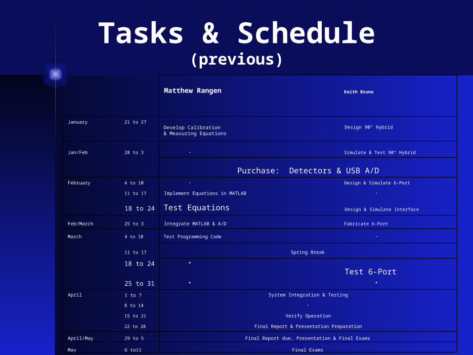
Tasks & Schedule(current)
Matthew Rangen Keith Bruno
January 21 to 27 Develop Calibration & Measuring Equations
Design & Simulate 90º Hybrid
Jan/Feb 28 to 3 · · February 4 to 10 · 11 to 17 Implement Equations in MAT LAB
Design & Simulate Lange Coupler
18 to 24 · · Feb/March 25 to 3 · Design & Simulate 6-port March 4 to 10 Test Programming Code · 11 to 17 Spring Break 18 to 24 · Fabricate 6-port Parts 25 to 31 Integrate MATLAB & Oscilloscopes Fabricate 6-port April 1 to 7 Purchase Detectors 8 to 14 Test 6-port 15 to 21 System Integration & Testing 22 to 28 Final Report & Presentation Preparation April/May 29 to 5 Final Report due, Presentation & Final Exams May 6 to11 Final Exams

Overview
• Objective
• Background
• Block Diagram
• Tasks & Schedule
• Current Results• MATLAB• Network Analyzer
• Future Work

Questions?
Check us out at:
cegt201.bradley.edu/projects/proj2005/sixpna
Recommended