Download pdf - Localization for the Next Generation of Autonomous Vehicles · Localization for the Next Generation of Autonomous Vehicles Chris Osterwood, CTO, Carnegie Robotics Fergus Noble, CTO,

Localization for the Next Generation of

Autonomous Vehicles

Chris Osterwood, CTO, Carnegie RoboticsFergus Noble, CTO, Swift Navigation

©2017 Swift Navigation. All rights reserved | Version 1.0 | 05.26.2017

www.swiftnav.com | @SwiftNav | [email protected]

Localization for the Next Generation of Autonomous Vehicles

2

SummaryThe next generation of autonomous systems, from commercial Unmanned Aerial Vehicles (UAVs) to outdoor ground robots to self-driving cars, will need much better localization accuracy than has traditionally been available. Additionally, high-volume autonomous systems and vehicles require a solution that is available at an acceptable price point. There has also been a lack of consensus around what combination of sensors will be required, especially for safety-critical applications that have to work in a wide range of conditions.

In this paper, we discuss the tradeoffs of varying sensor packages and demonstrate that precise Global Navigation Satellite Systems (GNSS), coupled with an Inertial Measurement Unit (IMU), provides the localization cornerstone for these systems. Precise knowledge of system position and attitude increases the utility of locally collected imagery and 3D sensors by reducing the computational cost of registering data with existing maps or previously collected data. Precise GNSS provides the system with global position while the IMU provides heading, pitch, and roll information while also allowing global position to be known by the system at 100 Hz or more.

We will present results from a low-cost Inertial Navigation System (INS) that incorporates Real Time Kinematic (RTK) GNSS and a Micro-Electro-Mechanical Systems (MEMS) IMU, showing that it provides excellent performance under a range of challenging conditions and is available at a fleet-friendly price-point.

IntroductionThe next generation of vehicles offering advanced driver assistance or fully autonomous operation will demand increasingly accurate position information, available in all driving conditions and with 100% availability. No single sensor is able to meet these requirements alone and therefore it is necessary to use a combined sensor suite solution incorporating a number of different kinds of sensors working together.

As the only source of absolute position, velocity and time, GNSS play a critical role in next generation positioning systems. However, typical GNSS are only capable of positioning to the road level with 2 - 5 meter accuracy. Enabling the next levels of autonomy (levels 3 - 5) requires lane-level positioning, which in turn requires a GNSS system with centimeter-level accuracy (10 cm).

To provide this increased level of performance, it is necessary to correct for several sources of error that typically limit the accuracy achievable with GNSS. It is also critical to provide this level of accuracy robustly, and without long solution convergence times, as is the case with many precision GNSS algorithms.

Additionally, use of inertial navigation systems technology, wherein GNSS information is augmented with local inertial measurements through accelerometers and gyroscopes, provides additional useful information like vehicle heading, as well as increasing the frequency,


3

A GNSS receiver determines its position by measuring its distance to four or more GNSS satellites. To determine its distance to the satellites, the GNSS receiver measures the phase of unique ‘codes’ continuously transmitted by the satellites. By comparing the relative phase offsets of the received codes, the receiver can determine the relative distance to each satellite, i.e. the distance to each satellite plus a common offset (the time of the measurement is unknown until solved for, leading to an unknown common offset to all the distances).

Once the relative distances to the satellites are known, the three-dimensional coordinates of the receiver and the time of the measurement can then be solved for via iterative algorithms.

Note that there are several GNSS in place around Earth that allow global position to be calculated. Satellite constellations that provide this capability include:

• GPS, owned by the United States government and operated by the United States Air Force. GPS has been in service since the early 1980s.

• GLONASS, operated by the Russian government.• Galileo, operated by the European Union, European Space Agency, and European GNSS

Agency.• BeiDou, operated by the China National Space Administration.

Overview of GNSS Technology

smoothness and robustness of the position information. This paper shows some initial results from the low-cost MEMS IMU on-board the Swift Navigation Piksi® Multi GNSS receiver when used with SmoothPose, a pose filter from Carnegie Robotics. Note that these results are from a limited number of tests and may not be representative of possible future products from Carnegie Robotics and Swift Navigation.

Figure 1. GPS receiver measuring the distances to four satellites; the minimum for a 3D position fix.


4

GNSS receivers can receive codes from just one constellation or from multiple constellations simultaneously. Receivers with multi-constellation capability generally have higher availability of position information due to the greater number of satellites they can use for position determination.

The phase of the code must be measured very precisely to correctly measure the distance to the satellite. In practice, there is a limit to the precision with which the code phase can be measured. Each bit of the codes transmitted by the satellites is quite long—about 300 meters in length. The 300-meter-units of the code bits combined with the imprecise code phase measurement leads to an upper bound on the accuracy with which the distance to the satellite can be measured—generally a few meters.

Figure 2. To determine the distance to a GNSS satellite, a GNSS receiver measures the phase of the code continuously transmitted by that satellite.

Each bit of the code is about 300 meters long.

Another important source of error is ionospheric delay. The ionosphere, a layer of charged particles surrounding the earth, slows the GNSS signals as they pass through it. This delay is hard to estimate and varies by time and location, leading to a few meters of error in the measurement of the distance to the satellite.

Figure 3. The ionosphere slows GNSS signals, adding a few meters of error in the distance measurement.


5

RTK GNSS systems are able to achieve much higher positioning precision by mitigating the sources of error described above.

Carrier MeasurementFirst, in addition to measuring the code phase, an RTK GNSS receiver measures the phase of the carrier wave upon which that the code is modulated. The carrier has a wavelength of about 19 centimeters. This makes it possible to measure to a much greater degree of accuracy than the 300 meter code.

However, there is a catch—there are an unknown number of whole carrier wavelengths between the satellite and receiver. Clever algorithms are required to resolve this “integer ambiguity” by checking that the code and carrier phase measurements lead to a consistent position solution as the satellites move and the geometry of the problem changes. During this time period of “integer ambiguity”, an RTK receiver is considered to be in RTK Float Mode and horizontal accuracy can range from 20 cm to 200 cm. Once the ambiguity is resolved, the RTK receiver will report that it is in RTK Fixed Mode and horizontal accuracy will be generally be 1 cm to 5 cm.

Overview of Precision GNSS Technology

Figure 4. The carrier, at 19 centimeters per wavelength,is much more precise than the code.

Reference ReceiverSecond, an RTK GPS receiver is able to reduce the ionospheric error with the help of an additional reference receiver. As long as the receivers are located relatively close to each other the ionospheric delay will be approximately the same for both receivers, and the difference in distance between the receivers to the satellite can be computed. Having the relative distances between the receivers to 4 satellites, a relative position between the receivers free of ionospheric error can be calculated.


6

Figure 5. An RTK system uses multiple receivers to minimize the effect of ionospheric delay and solve for the “integer ambiguity”.

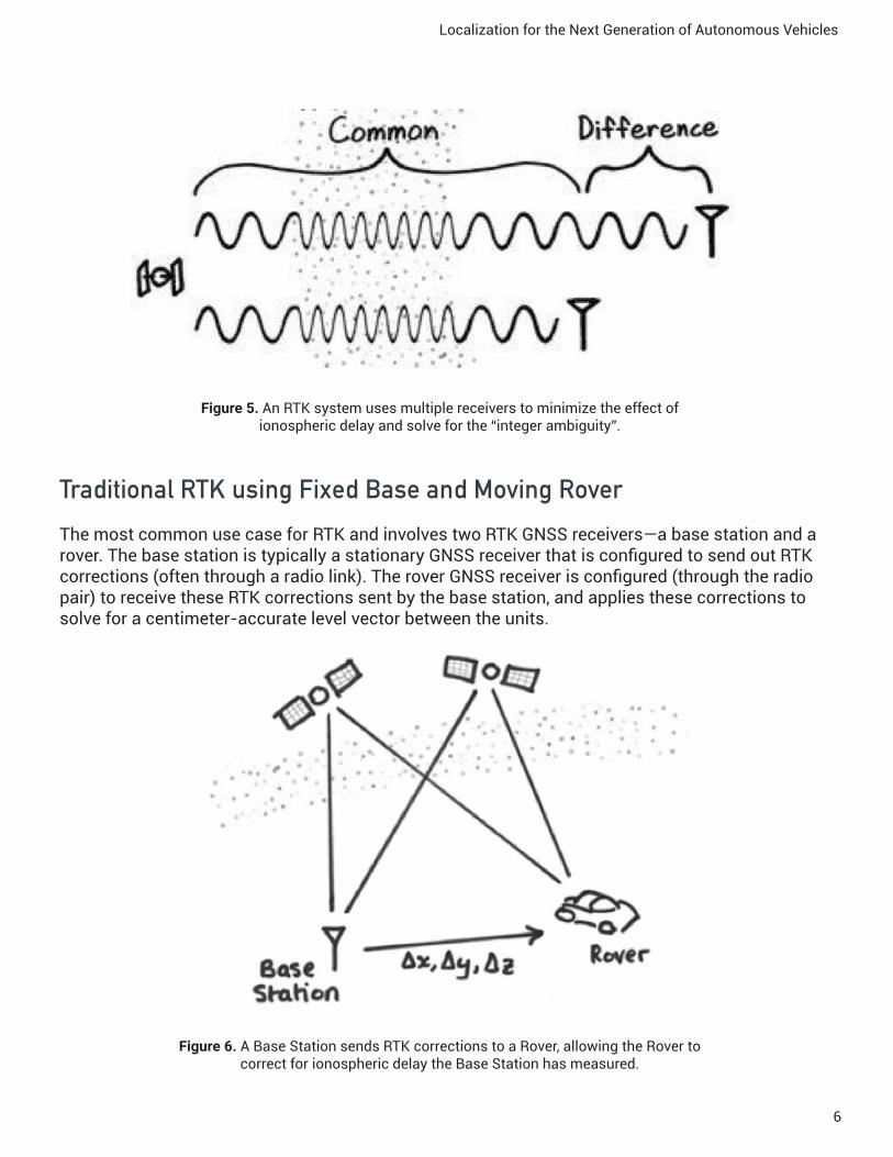
Traditional RTK using Fixed Base and Moving RoverThe most common use case for RTK and involves two RTK GNSS receivers—a base station and a rover. The base station is typically a stationary GNSS receiver that is configured to send out RTK corrections (often through a radio link). The rover GNSS receiver is configured (through the radio pair) to receive these RTK corrections sent by the base station, and applies these corrections to solve for a centimeter-accurate level vector between the units.

Figure 6. A Base Station sends RTK corrections to a Rover, allowing the Rover to correct for ionospheric delay the Base Station has measured.


7

RTK requires two independent GPS / GNSS receiver modules to be linked with a robust communication link so that the primary (Base Station) unit can send RTK corrections to the secondary (Rover) unit. The rover receives these RTK corrections and solves for a ‘vector’ ΔX, ΔY, ΔZ that is accurate to within 1-2 centimeters with reference to the base station unit. If one has accurately surveyed and entered the base station coordinates, then the rover shall use these base station coordinates to solve for its position in the global reference frame.

Standard GPS Receiver RTK GPS System

Number of GPS Receivers One: Roving Receiver Two: Roving Receiver and ReferenceReceiver

Position Type Absolute (Latitude, Longitude, Altitude)

Absolute (Latitude, Longitude, Altitude)

and

Relative (Vector between reference and rover)

Horizontal Position Accuracy 3 - 5 meters 1 - 5 centimeters

Vertical Position Accuracy 12 - 15 meters 2 - 15 centimeters


8

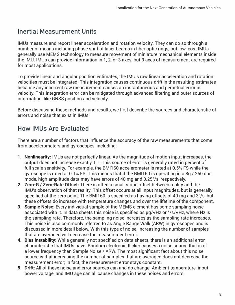
Inertial Measurement UnitsIMUs measure and report linear acceleration and rotation velocity. They can do so through a number of means including phase shift of laser beams in fiber optic rings, but low-cost IMUs generally use MEMS technology to measure movement of miniature mechanical elements inside the IMU. IMUs can provide information in 1, 2, or 3 axes, but 3 axes of measurement are required for most applications.

To provide linear and angular position estimates, the IMU’s raw linear acceleration and rotation velocities must be integrated. This integration causes continuous drift in the resulting estimates because any incorrect raw measurement causes an instantaneous and perpetual error in velocity. This integration error can be mitigated through advanced filtering and outer sources of information, like GNSS position and velocity.

Before discussing these methods and results, we first describe the sources and characteristic of errors and noise that exist in IMUs.

How IMUs Are EvaluatedThere are a number of factors that influence the accuracy of the raw measurements that come from accelerometers and gyroscopes, including:

1. Nonlinearity: IMUs are not perfectly linear. As the magnitude of motion input increases, the output does not increase exactly 1:1. This source of error is generally rated in percent of full scale sensitivity. For example, the BMI160 accelerometer is rated at 0.5% FS while the gyroscope is rated at 0.1% FS. This means that if the BMI160 is operating in a 8g / 250 dps mode, high amplitude data may have errors of 40 mg and 0.25°/s, respectively.

2. Zero-G / Zero-Rate Offset: There is often a small static offset between reality and the IMU’s observation of that reality. This offset occurs at all input magnitudes, but is generally specified at the zero point. The BMI160 is specified as having offsets of 40 mg and 3°/s, but these offsets do increase with temperature changes and over the lifetime of the component.

3. Sample Noise: Every individual sample of the MEMS element has some sampling noise associated with it. In data sheets this noise is specified as µg/√Hz or °/s/√Hz, where Hz is the sampling rate. Therefore, the sampling noise increases as the sampling rate increases. This noise is also commonly referred to as Angle Range Walk (ARW) in gyroscopes and is discussed in more detail below. With this type of noise, increasing the number of samples that are averaged will decrease the measurement error.

4. Bias Instability: While generally not specified on data sheets, there is an additional error characteristic that IMUs have. Random electronic flicker causes a noise source that is of a lower frequency than Sample Noise / ARW. The most significant fact about this noise source is that increasing the number of samples that are averaged does not decrease the measurement error; in fact, the measurement error stays constant.

5. Drift: All of these noise and error sources can and do change. Ambient temperature, input power voltage, and IMU age can all cause changes in these noises and errors.


9

As one would expect, there is a wide range of noise, error and drift ratings found in IMUs available in the marketplace. Higher-priced IMUs do perform better than less expensive IMUs, but the price-to-performance curve is steep. For comparison purposes, the BMI160 onboard the Piksi Multi is compared in the graphs and tables below with a MEMS IMU that costs 500x the BMI160.

A standard way to compare different noise and drift effects is the Allan Variance. It is a method of analyzing a data sequence in the time domain and enables visualization and quantification of Sample Noise and Bass Instability. Take the following steps to compute an Allan Variance:

1. An IMU is statically placed in a temperature controlled chamber and a long time history of accelerations and rotations is recorded. Generally, recording occurs for 24 hours.

2. A set of averaging times (taus) is selected, the plots below were generated with 30 different time intervals between 0.02 seconds and 4000 seconds.

3. For each averaging time (tau), stride over the time history and average samples within the window. All averages for each tau are then averaged to find the noise for that tau. The results are plotted on a log-log plot.


10

Figure 7. Allan Deviation plots for two Accelerometers and Gyroscopes

The minimum of the resulting curve is the component’s Bias Instability. Sample Noise will appear on the Allan Variance plot as a slope with gradient of -0.5. The measurement of Angular Random Walk (ARW) or is found by fitting a straight line through this slope and reading it’s value a tau = 1 second.

Low Cost MEMS High Cost MEMS

Measure Units X Y Z X Y Z

AccelBias Stability mg 0.029 0.074 0.043 0.022 0.037 0.031

VRW mg/√hr 6.6 7.9 8.5 2.8 3.0 2.8

GyroBias Stability °/hr 5.3 4.8 4.0 4.1 4.1 4.7

ARW °/s/√hr 0.36 0.31 0.30 0.30 0.26 0.30


11

As you can see from the Allan Variance and Summary Table above, the BMI160 gyroscope had similar performance to the high-cost IMU and the BMI160 accelerometer has about double the noise of the high-cost IMU. But, there are ways of correcting and compensating for IMU’s numerous noise and error sources. Without these corrections, low cost IMUs do not have enough accuracy to provide useful data over multi-second GNSS dropouts for accurate heading information.

Carnegie Robotics employs two main methods to improve IMU performance and accuracy. First, factory calibration of the IMUs allows good initial estimates of offset and scale factors for all axes of the accelerometer and gyroscope. This factory calibration can include calibration at high ambient temperatures to allow for compensation of temperature based scale and offset changes.

Second, the Extended Kalman Filter (EKF) in the Carnegie Robotics SmoothPose Filter continuously tunes these offset and scale factors for all axes of measurement. This online process is critical because the numerous noise and error sources cannot be independently measured nor isolated. As a result of this unknown coupling, no factory calibration can accurately correct raw measurements over the lifetime of the IMU. The EKF tunes these parameters through observation of the IMU and external inputs like GNSS-based position and velocity, as well as available vehicle odometry information.

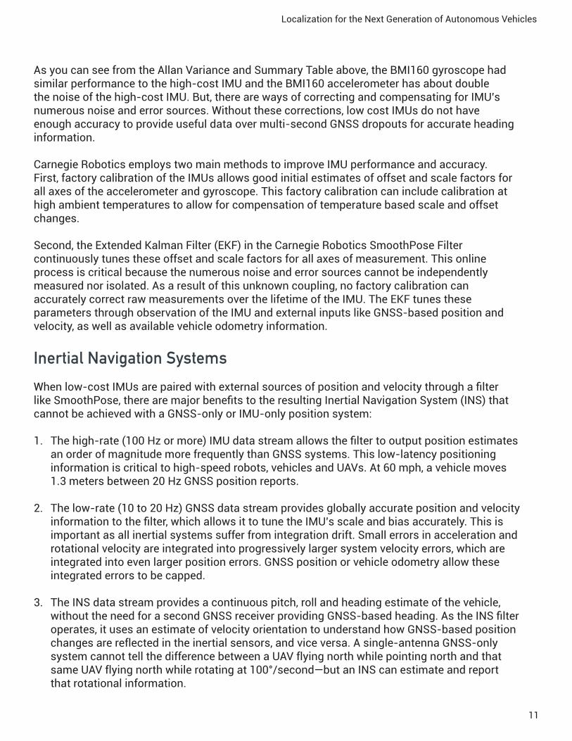
Inertial Navigation SystemsWhen low-cost IMUs are paired with external sources of position and velocity through a filter like SmoothPose, there are major benefits to the resulting Inertial Navigation System (INS) that cannot be achieved with a GNSS-only or IMU-only position system:

1. The high-rate (100 Hz or more) IMU data stream allows the filter to output position estimates an order of magnitude more frequently than GNSS systems. This low-latency positioning information is critical to high-speed robots, vehicles and UAVs. At 60 mph, a vehicle moves 1.3 meters between 20 Hz GNSS position reports.

2. The low-rate (10 to 20 Hz) GNSS data stream provides globally accurate position and velocity information to the filter, which allows it to tune the IMU’s scale and bias accurately. This is important as all inertial systems suffer from integration drift. Small errors in acceleration and rotational velocity are integrated into progressively larger system velocity errors, which are integrated into even larger position errors. GNSS position or vehicle odometry allow these integrated errors to be capped.

3. The INS data stream provides a continuous pitch, roll and heading estimate of the vehicle, without the need for a second GNSS receiver providing GNSS-based heading. As the INS filter operates, it uses an estimate of velocity orientation to understand how GNSS-based position changes are reflected in the inertial sensors, and vice versa. A single-antenna GNSS-only system cannot tell the difference between a UAV flying north while pointing north and that same UAV flying north while rotating at 100°/second—but an INS can estimate and report that rotational information.


12

4. As INS-based position estimates can be made between GNSS samples, they can similarly provide position estimates in the absence of GNSS data. This means that a robot or vehicle with an INS still has a position estimate as it drives under bridges, between tall buildings, in tunnels, and in other areas where not enough sky is visible for a GNSS solution. Of course, as the GNSS dropout duration increases, the INS-based position estimate accumulates more and more integration error, causing the estimate to be less accurate. In these instances, it is critical for the system-integrator to closely monitor the INS’ reported covariance to understand the certainty of the INS’ reported position and orientation estimate.

5. Lastly, an INS filter like SmoothPose can reject errant GNSS position and velocity reports caused by radio reflections off of buildings or a loss of sky reducing the number of visible satellites. An INS is able to do this because of the extra knowledge of vehicle motion provided by the IMU.

In the visualizations below, we present a few examples of an INS, consisting of Swift Navigation’s Piksi Multi and Carnegie Robotics’ SmoothPose, exhibiting these characteristics. In all of these maps, the red dots are GNSS position estimates at 20 Hz and the white dots are INS position estimates reported at 100 Hz. They are so dense that they look like a solid line.

Figure 8. Overview of the following INS examples along a single test path in Pittsburgh, PA.


13

Example 1. Tall buildings and “urban canyons” can cause errant GNSS position estimates due to radio reflections off of buildings and a loss of sky reducing the number of visible satellites. The INS data stream is accurate and

not affected by these errors.

Example 2. When the car passes underneath the highway overpass, the GNSS receiver loses visibility of the sky, reports positions inaccurately, and then not at all.

The INS initially estimates position accurately, but some of the incorrect GNSS reports cause the INS estimate to jump before recovering when the GNSS data stream resumes.


14

Example 3. Here the 20 Hz GPS data stream is visibly separated due to the high speed of the vehicle on the highway. The high rate INS provides lower-latency and

denser information.


15

Example 4. In this example, we induce an artificial GNSS dropout while still displaying the GNSS data in the maps view. However, the INS system has no GNSS data for 60 seconds and is only estimating vehicle

position from IMU observations. Over this time period one can see visible integration error, particularly in the direction of motion due to the double integration of the accelerometer and the highway vehicle speed.