Localization for Autonomous Vehicles

Thesis for the Degree of Licentiate of Engineering

Localization for Autonomous Vehicles

Erik Stenborg

Department of Electrical EngineeringChalmers University of Technology

Göteborg, Sweden 2017

Localization for Autonomous VehiclesErik Stenborg

c© Erik Stenborg, 2017.

Technical report number: R012/2017ISSN 1403-266X

Department of Electrical EngineeringSignal Processing GroupChalmers University of TechnologySE–412 96 Göteborg, Sweden

Typeset by the author using LATEX.

Chalmers ReproserviceGöteborg, Sweden 2017

Abstract

There has been a huge interest in self-driving cars lately, which is under-standable, given the improvements it is predicted to bring in terms of safetyand comfort in transportation. One enabling technology for self-drivingcars, is accurate and reliable localization. Without it, one would not beable to use map information for path planning, and instead be left to solelyrely on sensor input, to figure out what the road ahead looks like. Thisthesis is focused on the problem of cost effective localization of self-drivingcars, which fulfill accuracy and reliability requirements for safe operation.

In an initial study, a car equipped with the sensors of an advanced driver-assistance system is analyzed with respect to its localization performance. Itis found that although performance is acceptable in good conditions, it needsimprovements to reach the level required for autonomous vehicles. Theglobal navigational satellite system (GNSS) receiver, and the automotivecamera system are found to not provide as good information as expected.This presents the opportunity to improve the solution, with only marginallyincreased cost, by utilizing the existing sensors better.

A first improvement is regarding global navigational satellite systems(GNSS) receivers. A novel solution using time relative GNSS observations,is proposed. The proposed solution is tested on data from the DriveMeproject in Göteborg, and found capable of providing highly accurate time-relative positioning without use of expensive dual frequency receivers, basestations, or complex solutions that require long convergence time. Errorintroduced over 30 seconds of driving is found to be less than 1 dm onaverage.

A second improvement is regarding how to use more information fromthe vehicle mounted cameras, without needing extremely large maps thatwould be required if using traditional image feature descriptors. This shouldbe realized while maintaining localization performance over an extendedperiod of time, despite the challenge of large visual changes over the year.A novel localization solution based on semantic descriptors is proposed,and is shown to be superior to a solution using traditional image featuresin terms of size of map, at a certain accuracy level.

i

List of appended papers

Paper I M. Lundgren, E. Stenborg, L. Svensson and L. Hammarstrand, "Ve-hicle self-localization using off-the-shelf sensors and a de-tailed map", 2014 IEEE Intelligent Vehicles Symposium, Proceed-ings pages 522-528.

Paper II E. Stenborg and L. Hammarstrand, "Using a single band GNSSreceiver to improve relative positioning in autonomous cars",2016 IEEE Intelligent Vehicles Symposium, Proceedings pages 921-926

Paper III E. Stenborg, C. Toft and L. Hammarstrand, "Long-term VisualLocalization Using Semantically Segmented Images", Submit-ted to 2018 IEEE International Conference on Robotics and Automa-tion

ii

Preface

More than four years ago, when I was about to start this project, I thought,"Localization is almost solved, and what little remains ought to be easy!Five years is way too much time allocated - what am I going to do afterthree years when the problem is solved, and the DriveMe cars are roamingthe streets of Göteborg with my code in them?". Now, almost five yearslater, I’m very happy that I’ve reached this half-way milestone, that theLicentiate thesis marks, and I wonder if I’m ever going to make a dent inthe mountain of work that remains until the problem really is solved.

I have learned a lot, though. I have learned that research takes time.I have learned that the path to success is full of failures that nobody sees,but the person who makes them. I have learned that all those failures ispart of the process. And I have learned to appreciate the advice from thosewho have gone through the process, and emerged successfully on the otherend, a little bit wiser than the rest of us who are in the middle of it.

I would like to show my gratitude towards my academic supervisorsLennart Svensson and Lars Hammarstrand for your advise, for your unwa-vering support, for our interesting discussions about both professional andother matters, and for all help I have received to reach this milestone. Avery big thanks also to my industrial supervisor Joakim Sörstedt and mymanager Jonas Ekmark for giving me this opportunity, for your enthusiasm,for your support of my work, and for believing in me. I would also like tothank Vinnova, Volvo Car Corporation and Zenuity for financing my work.

Thanks to all friends and colleagues (both in the past and the present)in the signal processing and the image analysis groups at Chalmers, at theactive safety department at Volvo and at Zenuity. Lunches and fika wouldn’tbe nearly as entertaining without you. Special thanks to Malin, for helpingme getting started when I first joined the group at Chalmers and for co-authoring the very first published paper with my name on it, to Carl forbeing such a rock and helping me with my present work, to Anders for beinga good room mate and accepting my quirks (I apologize for shooting youthe first day we met). Special thanks also to Karl, Abu, Maryam, Daniel,Samuel, Erik, Yair, and all the rest of you already mentioned, for proofreading or otherwise helping me with this thesis and the papers in it.

A warm thanks to my parents. Without you, I literally wouldn’t be heretoday. Finally, I would like to extend a very warm thanks to my belovedwife, Yoko, and to my lovely daughters, Lina and Hanna, for being such awonderful family. I love you.

Erik StenborgGöteborg, 2017

iii

iv

Contents

Contents v

I Introductory Chapters

1 Introduction 1

2 Localization 51 Overview . . . . . . . . . . . . . . . . . . . . . . . . . . . . . 52 Map representation . . . . . . . . . . . . . . . . . . . . . . . 83 Accuracy requirements . . . . . . . . . . . . . . . . . . . . . 9

3 Sensors and observations 111 Global Navigation Satellite System . . . . . . . . . . . . . . 132 Camera . . . . . . . . . . . . . . . . . . . . . . . . . . . . . 183 Radar . . . . . . . . . . . . . . . . . . . . . . . . . . . . . . 23

4 Filtering and smoothing 251 Problem formulation and general solution . . . . . . . . . . . 262 Kalman filter . . . . . . . . . . . . . . . . . . . . . . . . . . 273 Unscented Kalman Filter . . . . . . . . . . . . . . . . . . . . 284 Particle filters . . . . . . . . . . . . . . . . . . . . . . . . . . 305 Smoothing and mapping . . . . . . . . . . . . . . . . . . . . 31

5 Contributions and future work 35

II Included Papers

Paper I Vehicle self-localization using off-the-shelf sensors anda detailed map 491 Introduction . . . . . . . . . . . . . . . . . . . . . . . . . . . 492 Problem formulation . . . . . . . . . . . . . . . . . . . . . . 50

v

Contents

3 Generating a map . . . . . . . . . . . . . . . . . . . . . . . . 523.1 Lane markings and the reference route . . . . . . . . 523.2 Radar landmarks . . . . . . . . . . . . . . . . . . . . 53

4 Proposed solution . . . . . . . . . . . . . . . . . . . . . . . . 534.1 The state vector . . . . . . . . . . . . . . . . . . . . . 544.2 Process model . . . . . . . . . . . . . . . . . . . . . . 554.3 GPS measurement model . . . . . . . . . . . . . . . . 554.4 Measurement models for speedometer and gyroscope 564.5 Camera measurement model . . . . . . . . . . . . . . 564.6 Radar measurement model . . . . . . . . . . . . . . . 58

5 Evaluation . . . . . . . . . . . . . . . . . . . . . . . . . . . . 595.1 Implementation details . . . . . . . . . . . . . . . . . 595.2 Performance using all sensors . . . . . . . . . . . . . 605.3 Robustness . . . . . . . . . . . . . . . . . . . . . . . 61

6 Conclusions . . . . . . . . . . . . . . . . . . . . . . . . . . . 61

Paper II Using a single band GNSS receiver to improve rela-tive positioning in autonomous cars 711 Introduction . . . . . . . . . . . . . . . . . . . . . . . . . . . 712 Problem formulation . . . . . . . . . . . . . . . . . . . . . . 73

2.1 Information sources . . . . . . . . . . . . . . . . . . . 743 Models . . . . . . . . . . . . . . . . . . . . . . . . . . . . . . 76

3.1 Measurement models . . . . . . . . . . . . . . . . . . 763.2 Augmented state vector and process model . . . . . . 79

4 Implementation and evaluation . . . . . . . . . . . . . . . . 804.1 Scenario . . . . . . . . . . . . . . . . . . . . . . . . . 804.2 Results . . . . . . . . . . . . . . . . . . . . . . . . . . 81

5 Conclusions . . . . . . . . . . . . . . . . . . . . . . . . . . . 82

Paper III Long-term Visual Localization Using SemanticallySegmented Images 891 Introduction . . . . . . . . . . . . . . . . . . . . . . . . . . . 892 Problem statement . . . . . . . . . . . . . . . . . . . . . . . 91

2.1 Observations . . . . . . . . . . . . . . . . . . . . . . 912.2 Maps . . . . . . . . . . . . . . . . . . . . . . . . . . . 932.3 Problem definition . . . . . . . . . . . . . . . . . . . 93

3 Models . . . . . . . . . . . . . . . . . . . . . . . . . . . . . . 933.1 Process model . . . . . . . . . . . . . . . . . . . . . . 933.2 Measurement model . . . . . . . . . . . . . . . . . . 94

4 Algorithmic details . . . . . . . . . . . . . . . . . . . . . . . 964.1 SIFT filter . . . . . . . . . . . . . . . . . . . . . . . . 964.2 Semantic filter . . . . . . . . . . . . . . . . . . . . . . 97

vi

Contents

5 Evaluation . . . . . . . . . . . . . . . . . . . . . . . . . . . . 995.1 Map creation . . . . . . . . . . . . . . . . . . . . . . 995.2 Ground truth . . . . . . . . . . . . . . . . . . . . . . 100

6 Results . . . . . . . . . . . . . . . . . . . . . . . . . . . . . . 1017 Discussion . . . . . . . . . . . . . . . . . . . . . . . . . . . . 101

vii

viii

Part I

Introductory Chapters

Chapter 1

Introduction

Autonomous vehicles have several advantages to vehicles which must bedriven by humans, one being increased safety. Despite an increase in numberof cars and total distance driven, traffic injuries has declined in Sweden [1]and the USA [2], from being the leading cause of death in age groups below45, to "merely" being in the top ten [3]. To continue this trend, we increasethe scope of traffic safety from just protecting passengers in case of anaccident, to mitigating or preventing accidents before they happen. Basedon studies such as [4], where it is noted that a vast majority of accidentsare caused by human error, we can see that the largest potential to furtherincreased safety, lies in letting technology assist drivers by automating thedriving task, and thus creating self-driving cars.

Other reasons for self-driving cars are economy, as people can be moreproductive while on the road; equality, as blind and otherwise impairedpeople then can ride by themselves; and also environment, since the needfor parking in cities could be reduced if all cars could leave by themselvesafter the rider has reached the destination.

Now, let us look into the problems we need to solve to make autonomousvehicles available. These problems include human factors, economy, legalliability, equality, morality, etc. This thesis focuses on technical problems,specifically those regarding precise localization. Economy and safety re-strict possible solutions, but apart from that, we can view the problem oflocalization independently. The technical problem of autonomous drivingcan be described as a function which maps sensor data to control signals forthe car, primarily wheel torque for longitudinal acceleration and steeringtorque for turning the car. The rest which needs controlling in the car, e.g.controlling flow of fuel and air to the engine, is already solved.

There are several possible ways in which we can approach this problemof mapping sensor data to control outputs. One possibility is to decide on asensor setup that seems reasonable, e.g., a set of cameras based on the fact

1

Chapter 1. Introduction

Map

Sensors

Perception

Prediction

Planning

Actuation

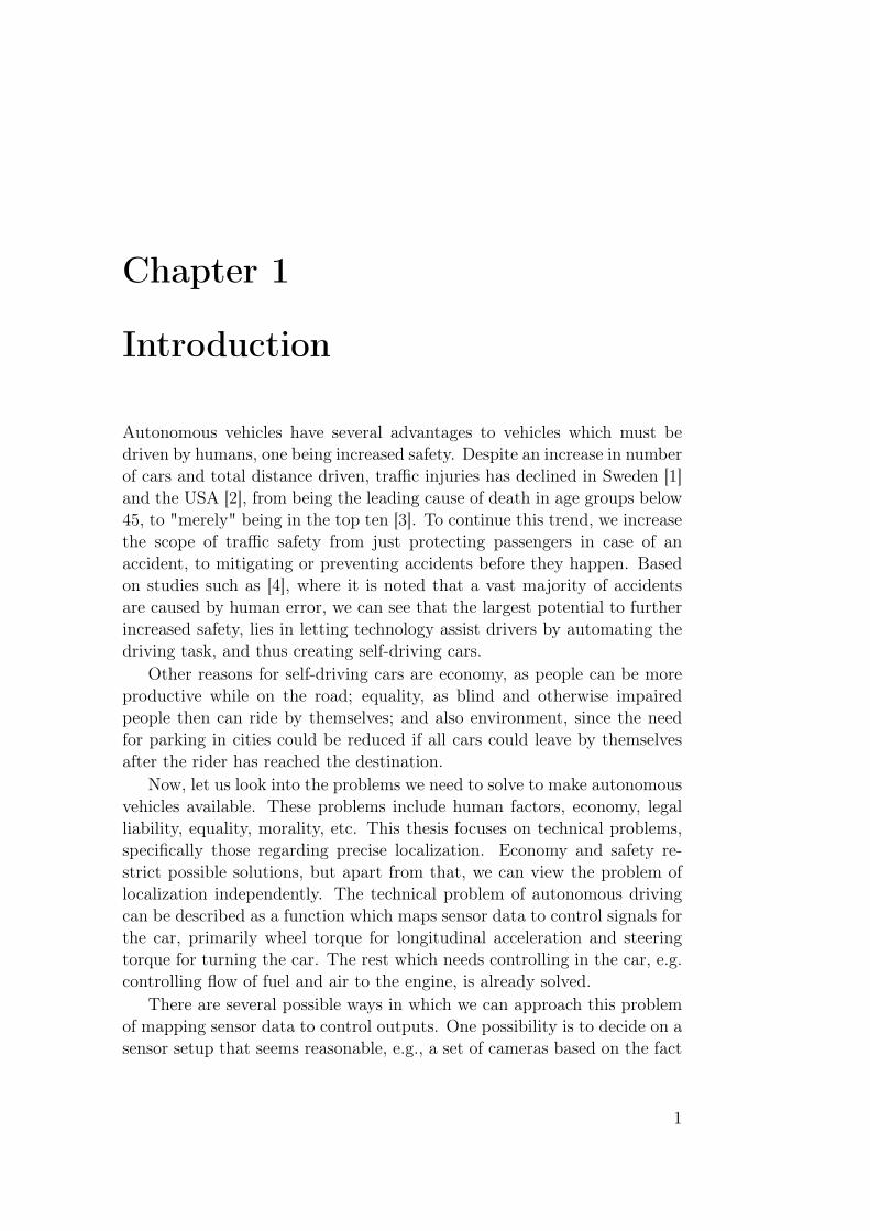
Figure 1.1: Flow of data and processing modules for autonomous driving.Localization is here considered part of the perception module.

that humans are able to drive a car mainly based on vision input, and thentreat it as a machine learning problem, using either reinforcement learningor supervised learning with a human expert driver. This approach has sofar rendered some success [5–7], but most larger scale projects are focusingon more modular approaches where the driving task is divided into smallerparts, which can be designed and verified more independently of each other.

In the modular approach, the problem is subdivided into a few majormodules, where Figure 1.1 shows one example of such a subdivision. Wehave one module which is responsible for planning a trajectory and followingit based on information from the other modules, another which interpretsthe sensor inputs into a simple structure that is meaningful for the drivingtask, and a third which predicts what other traffic participants will do. Theoutput from the perception block will typically contain information aboutboth the dynamic environment, such as position and velocity of other roadusers, and the static environment, such as which areas are drivable andwhich contain static obstacles.

When it comes to describing the static environment, there are twoparadigms. One is to rely only on the input provided by the sensors onthe own car, and the other is to rely also on a predefined map and relatingthe sensor inputs to that map. The map paradigm will provide more in-formation about the static environment than what is visible using only thesensors, and is thus often preferred. However, to use a map, one must beable to localize the car in the map. Any uncertainty in position and orienta-tion in relation to the map will translate into uncertainty about the drivablearea and in consequence also the planned path. Thus, we can see that ac-

2

curate localization in relation to an accurate map of the close surroundingsof the car, is an enabler for autonomous driving.

Then what is needed to solve effective localization for autonomous ve-hicles? Firstly, we need to understand what is needed in terms of accuracy,availability and price. These requirements are far from obvious, and couldwarrant a thesis in and by itself, but a short description of how one canreason about it is included in Chapter 2. Secondly, we need a map thatconnects the observable landmarks with the possibly unobservable, staticfeatures of the road that are needed for path planning, i.e. drivable surface,static obstacles, etc. A few thoughts on this map have also been includedin Chapter 2. Thirdly, we need sensors which are capable of observing thelandmarks, and sensor models which describe how the observations relateto the physical world. In Chapter 3, radars are briefly described, whilecameras and global navigation satellite systems such as GPS, are describedin further detail, with a focus on how they can be used for localizationpurposes. Lastly, we need algorithms that combine the given maps and themeasurements into estimates of position and orientation. This is achievedusing the Bayesian estimation framework described in Chapter 4, where wesee how to combine the models of various sensors with a motion model forthe vehicle to arrive at probabilistic models of position and orientation.

This thesis examines what level of localization accuracy that can beachieved using different types of automotive classified sensors. It furtherestablishes a few missing pieces in reaching desired performance, and pro-poses solutions for some of them. This is done in three separate papers,briefly summarized in Chapter 5.

3

4

Chapter 2

Localization

As concluded in the introduction, accurate localization with respect to amap is a key enabler for using information from those maps in the motionplanner. In this chapter we start with a brief overview of the research area,then have a look at what goes in the map, then look at how to use themap for localizing with respect to the drivable area, and finish by reasoningabout how to derive requirements on accuracy and availability.

1 Overview

If we look at the problem of localization with a given map in a slightly largercontext than for autonomous vehicles, we realize that it can be formulated inmany different ways. We can roughly categorize problems in four categories,based on two criteria: metric vs. topological, and single shot vs. sequential.In Table 2.1, the references given below are categorized in either of the fourcategories.

The first division between metric or topological localization is regardingthe result of the localization. Topological localization is when the resultof localization is categorical and can be represented as nodes in a graph,e.g., a certain room in a house, or the location where an image from atraining data set was taken. Examples here include place recognition byimage retrieval methods, where an image database of geo-tagged images isused to represent possible locations, and then a query image is comparedto the images in the database, and the most similar image along with itsposition is retrieved, see e.g., [8, 9]. Specialized loop closure detectors alsobelong in this category, see e.g., [10, 11]. These provide information to alarger system doing simultaneous localization and mapping (SLAM), whena robot has roughly returned to a previously visited place just by lookingat image similarities. In this category, there are also some solutions which

5

Chapter 2. Localization

topological metricsingle shot / global [8–11] [15–17, 19, 20]

sequential / with prior [12–14] [21–23, 27, 28]

Table 2.1: Classification of localization problems with a few examples ofproposed solutions.

focus on robust localization in conditions with large visual variations, seee.g., [12, 13]. They make use of sequences of images which as a groupshould match a sequence of training images in an image similarity sense.One could also argue that some hybrid methods, such as [14], belong in thiscategory, even though they claim to be "topometric" in the sense that theyprovide interpolation between the nodes in the graph and thus give metriclocalization result along some dimensions where a whole array of trainingimages has been collected.

Metric localization is more geometric in nature. The resulting locationis in a continuous space, and most easily expressed in coordinates using realnumbers. There are examples from the computer vision community thatdoes direct metric localization using a single query image, see e.g., [15–18],but also examples where a form of topological localization is performed firstas an initial step, see e.g., [19, 20]. Most localization in robotics, with thepurpose of providing navigational information to a robot, requires metriclocalization, with some examples in [21–23]. Localization using global satel-lite navigational systems and inertial measurement units are also examplesof metric localization.

The second division we have when categorizing localization, is betweensingle shot localization and sequential localization. This is regarding whattype of information is used for the localization. Single shot localizationuses only one observation and no additional information from just before orafter. This is relevant when using single images, see e.g., [8, 9, 11, 15–20],and sometimes also when using sensors that are specialized for localization,such as the global navigation satellite systems, see e.g., [24].

Sequential localization means using a sequence of observations and somemotion model to connect them, or alternatively, to have useful prior knowl-edge on the location from some other source. This is the type of observationsavailable for on-line robot navigation, see e.g., [12, 13, 21–23, 25–28]. Wenote that the type of localization needed for autonomous vehicles falls inthe intersection of sequential localization and metric localization. Thus, therest of the thesis will focus on metric, sequential localization.

Localization for autonomous vehicles has been done for quite some timeusing expensive sensor setups, including survey grade GNSS receivers, fiber

6

1. Overview

optical inertial measurement units and multi beam rotating laser scanners.Some of the most well known examples are the contributions to the DARPAGrand Challenge in 2005, see e.g., [25], and the DARPA Urban Challengein 2007, see e.g., [26]. Some spin-offs from these DARPA challenges, suchas Waymo, use similar technology, arguing that the cost of sensors will fallenough to make it viable for consumers in a near future. Others argue thatmore simple sensors should be enough for accurate and robust localization,but this is yet to be shown in practice. This cost constraint is the reasonthat this thesis is focused on solutions using sensors that are expected tobe readily available in future cars.

Localization with a given map, and mapping given known positions andorientations, are considered subproblems to the more general problem ofsimultaneously estimating both location and map (SLAM). See e.g. [29,30] for a survey of the SLAM problem. Although localizing with a givenmap would be sufficient for an autonomous vehicle, there is still a needto build the map and keep it updated. To keep costs down, this shouldshould be performed without huge fleets of special mapping vehicles usingvery expensive positioning systems. Thus, viewing both the localizationand mapping problems as SLAM problems is attractive from economicalreasons, in spite of it being slightly more complicated.

In the 1990’s, SLAM was usually solved using extended Kalman filters,see e.g., [31, 32], where the state vector described the location of landmarksof the map and the most recent robot location. There were both convergenceand scalability issues with this approach, due to a fixed linearization point,and an ever growing landmark covariance matrix that needed inverting inevery update. In 2002, solutions using particle filters [33] were presented.They provided better performance for larger problems, due to not havingto encode the correlation between landmarks, since they are conditionallyindependent given the robot trajectory. A few years later the trend shiftedtowards viewing the SLAM problem as a continuously growing smoothingproblem, as in e.g., GraphSLAM [34], and iSAM [35, 36]. This is still howit is typically solved today, see e.g. [37, 38] for some more recent work.For people with a background in computer vision rather than robotics, itcould be worth noting that, when using point features from camera imagesin GraphSLAM or iSAM, the solution is virtually identical to continuouslysolving a growing bundle adjustment problem with optimization methodsthat consider the sparse and incremental nature of the problem [39, 40].

7


2 Map representation

As previously noted, the problem in this thesis is self localization for au-tonomous vehicles using automotive grade sensors, and a map. For this weneed a map, and although we have hinted that this can be solved usingSLAM, it could be useful to discuss what to put in the map.

We know that the path planner needs some navigation information, e.g.,drivable area, lane connectivity, traffic rules, suitable speed profiles, etc., todo its job. This navigational information is connected to positions in theworld through markings on the ground, and traffic signs, which can be ob-served by a forward looking camera. These cues are what we would liketo localize with respect to. However, some sensors, e.g., cameras lookingbackwards, radars, or GNSS receivers, can not directly observe them. In-stead we may choose to use some other observable landmarks, and encodetheir relation to the navigational information in the map. With a mapthat holds both the navigational information needed by the path planner,and observable landmarks, the car can use on-board sensors to detect angleand/or range to the landmarks, and triangulate a position relative to thenavigational information in the map.

Now, these observable landmarks that we choose to add to the mapcan be quite sensor specific. Although geometric features, such as pointsor curves, are a popular choice, there are plenty of other options. Onealternative is a grid map, where the world is discretized in a 2-D or 3-D grid,where each pixel (or voxel in the 3-D case) describes some property aboutthat small part of the world. An often used property is occupancy, i.e., ifthe grid cell is transparent or opaque to the relevant sensor, often indicatingthat the cell is empty or occupied, hence its name [41, 42]. Another propertythat has been used successfully with grid maps is reflectivity, as in e.g., [43].A version of grid mapping that has been popularized with the introductionof the Kinect RGB-D camera, is the truncated signed distance function.Here, each voxel stores the signed distance to the nearest opaque surface,if it is below some threshold distance. In indoor environments, where thesize of the map is quite limited, 3-D grid maps have been demonstratedwith impressive results. However, a grid representation of the world scalesbadly with the number of dimensions to be described, and although workhas been done to compress the 3-D grids maps, see e.g., [44], most oftenthis approach is used for 2-D maps.

For large 3-D maps, a more common approach is to store sparse featuresthat are possible to describe with a few parameters. Points, lines, and B-splines are popular, but not the only possible choices. When using thesetypes of features, we should take care to construct feature detectors that

8

3. Accuracy requirements

are able to reliably detect these features in the sensor data.

Reference frame

For the motion planner, the only relevant information needed is the relativeposition from ourselves to other traffic participants, and to relevant objectsin the immediate surroundings. Where the origin of the metric map of theworld lies is irrelevant, as long as all relative positions and angles are correct.For most sensors, especially the cameras and radars used in this thesis, thisis also true. However, GNSS provides global localization with respect to acertain origin of the Earth, and thus, if we want to use GNSS to localizein the map, the map must be aligned to the world origin as defined by thecoordinate system used in GNSS.

Historically, maps have been thought of as 2-D projections of the surfaceof the Earth to a flat surface, such as a piece of paper or a screen. Itis mathematically impossible to map the surface of a sphere to a planewithout distortions and discontinuities, but there has been many proposalsfor suitable projections that does this without too much distortion, or withsome special property preserved at the expense of some other error beingintroduced.

For our needs, however, we can drop the requirement that the map mustproject well to a 2-D plane. We are merely interested in using the map forlocalization and path planning, and for that we need to keep track of 3-Dposition of landmarks, and the road. The map must at least be able to storea 3-D representation of landmarks and the road, in any part of the worldwithout discontinuities.

The most straight forward reference frame for a global 3-D map is anEarth centered and Earth fixed (ECEF) Cartesian coordinate frame that fol-lows the rotation of the Earth. In this coordinate system there are no prob-lems to map even Scott-Amundsen station at the south pole without discon-tinuities, and the transformation to a local east-north-up (ENU) frame is asimple rotation and translation. In the experiments in this thesis, however,the area where the car is driving is small enough, that a map in the localENU frame, with a flat Earth assumption, is sufficient.

3 Accuracy requirements

Now, let us look into what performance we require of our localization. Whataccuracy of localization is needed for autonomous driving? How often andlong can the localization be allowed to have an error over a certain threshold,and what is that threshold? These are difficult questions to answer, but in

9


order to evaluate performance, it is important to at least have an idea ofthe magnitudes, and a method to argue about them.

One possible starting point is a safety analysis. There are tools andframeworks to aid in such analysis, and they help us through hazard analysisand risk assessment to identify critical scenarios and the safety goals thatarise from them. The hazards are classified according to their risk, whichleads to a classification also of the safety goals. The ISO standard 26262defines five Automotive Safety Integrity Levels (ASIL): QM, A, B, C, and D,with D being the highest level. The classification is based on how frequentthe situation is (exposure), how severe the damages would be, and howcontrollable the situation is by the driver.

Let us take an example with the hazard of drifting out of the lane ina curve and colliding with oncoming traffic at 20 m/s or higher when inautonomous mode. This hazard is very severe in terms of expected dam-ages to the people involved in a head on collision, the situation is quitefrequent (high exposure), and it has low controllability since the driver isnot expected to be alert when the car is in autonomous mode. Thus, it getsthe highest classification, ASIL D, which roughly translates to a desired fre-quency of error of less than 1 in 1000 years. Next, we can split the hazardinto a fault tree, which should contain all possible faults that could causeit. There can be several possible causes, e.g., skidding if there is ice, notgetting enough steering torque from the power steering, or lane informationreported to the path planner being wrong. If the lane information is basedonly on using a map and localization, with ASIL D, both the map and thelocalization are required to give a lateral error that is small enough suchthat the vehicle does not cross over to the other lane (∼1 m).

This margin applies to the combined error of all components in the au-tonomous car, from sensing to actuation. To get the requirements for aspecific module in the chain of modules presented in Figure 1.1, one couldsubtract the error introduced by the last module of the chain, and thenpropagate the remainder backwards through the various transformationsthat each block causes. Localization resides in the perception module, earlyin the chain, and this type of backwards propagation of permissible errorcould be quite cumbersome. A slightly less difficult way to get a roughunderstanding of the error margins, could be to simulate errors in the local-ization and propagate them forward to see what the final control error willbe.

10

Chapter 3

Sensors and observations

When self-localization of cars is the topic, people often come to think of aGlobal Navigation Satellite System (GNSS), often the Global PositioningSystem (GPS), which has as its main purpose to measure position of thereceiver. However, as we have seen, there are also other sensors, primar-ily used for other purposes, which can be quite useful also for localization.Cameras and radars, as examples of this type of sensors, are primarily usedto detect obstacles and other road users in the local environment around thecar, and often more than one of each is required to get a good enough un-derstanding of the surroundings. Together with GNSS, and motion sensorssuch as accelerometers, gyroscopes and wheel speed sensors, they providethe measurements that we use for localization.

So, how do these sensors work, and how do we use them for localization?One common factor is that they capture electromagnetic waves (light orradio) that was either transmitted or reflected by some object in the en-vironment. They typically record the angle of arrival, or measure distanceto the object by recording the time delay of the captured signal. Some-times the intensity, and possibly some other features of the signal are alsorecorded. With sensors measuring angle to landmarks, the known positionsof the landmarks can be used to triangulate the ego-position, see Figure3.1. With sensors measuring distance, trilateration is used, see Figure 3.2.In both cases more than one landmark has to be detected to calculate anunambiguous position. In this chapter we look into more details on how thesensors used for localization in this thesis work, and how the measurementsare modeled.

11

Chapter 3. Sensors and observations

1 landmark 2 landmarks

Figure 3.1: Triangulation from landmarks with known positions. With onlyone landmark, there is no unique solution, but with two landmarks we geta unique solution in 2-D.

1 landmark 2 landmarks

Figure 3.2: Trilateration from landmarks with known positions. With onlyone landmark, again there is no unique solution, and with two landmarkswe get two possible positions in 2-D, but no information about orientation.

12

1. Global Navigation Satellite System

1 Global Navigation Satellite System

GNSS is, in a localization context, a rather unique sensor compared toother sensors. Its sole purpose is localization, while cameras and radars areprimarily used in the self-driving car for their ability to detect obstacles andother road users. GNSS is also the only sensor which has a global frame ofreference.

All GNSS systems, including GPS, which is the most well known, use thesame principle of positioning. Kaplan and Hegarty describe this in detail intheir book [45]. Essentially, a number of satellites with accurately knownEarth orbits, transmit signals at very well defined times, and the receiversmeasure the delay from the transmission to the reception. From this delaythe receiver can calculate the range to the satellite. By using multiplesimultaneous satellite observations, the receiver is able to trilaterate itsposition.

Coarse/acquisition (C/A) code ranging

The signal that is transmitted from the satellite consists of a carrier signal,on top of which there are up to two other signals, modulated using BinaryPhase Shift Keying. One of the signals is a repeating sequence of pseudorandom numbers, which functions as a unique identifier for the satellite,and is also what is used for range calculations. The other signal, whichis transmitted at a slower bit rate, is the navigational message. It pro-vides information about the satellite such as its status, orbital parameters,corrections to its clock, etc.

The normal method for determining position using GPS uses the se-quence of pseudo random numbers to calculate a pseudo range from thereceiver to the satellite. Since the sequence of pseudo random numbers(C/A code) is known in advance by the receiver, this can be done with atracking loop that calculates how much a local copy of the C/A code mustbe time shifted to match the received signal, see Figure 3.3. If the receiverhad a perfect clock, and if smaller error sources are ignored, one could sim-ply multiply the time shift with the speed of light to get the distance tothe satellite. Given three such measurements to different satellites, the 3-Dposition of the receiver could be trilaterated. However, the clock in a typicalreceiver is of relatively low quality, which is why the receiver time must alsobe treated as an unknown variable. That increases the requirement to foursatellites, in order to calculate a solution for position and time. This is thebasic idea of how simple positioning using the C/A code in GPS works. If areceiver does not make use of the carrier phase to smooth the pseudo rangemeasurements from the C/A code, there is a noise floor of around 1% of

13


Δt

Figure 3.3: The time offset, ∆t, when matching pseudo random numbersin the received C/A code signal to the internally generated sequence, isunique.

the bit length in the code, which is difficult to get below. The bit lengthis calculated as the bit length in seconds times the speed of light, and isaround 300m. This means that the receiver tracking loop introduces noiseon the pseudo range measurements that has a standard deviation of about3m. However, since modern receivers use some tricks, such as carrier phasesmoothing [46], the receiver noise is usually quoted as much lower today,see Table 3.1. Apart from the receiver tracking noise, there are other errorsaffecting the pseudo range measurements, leading to an average error thatis typically quoted as around 7 m, for a standard single frequency receiver.

Carrier phase ranging

Now, consider the carrier signal, which has a wavelength of about 0.2 m;much shorter than the bit length of the C/A code. If the tracking loops inthe receiver are able to determine the phase of the carrier signal within 1%,and if there is a way to remove additional errors, then potentially a veryaccurate range measurement to the satellite can be obtained.

The alignment to the carrier phase through phase lock loops in thereceiver, is indeed accurate to about 1 mm. However, there is now anotherproblem. Every cycle of the carrier signal looks the same. This meansthat if we examine the cross correlation between the received signal andthe internal oscillator, we would find an infinite number of peaks with aspacing that corresponds to the wavelength of the carrier signal. Whichpeak the phase lock loop locks on to, is random. This causes the rangemeasurement using the carrier phase, to be offset by an unknown integer Ntimes the wavelength. This integer, N , must be determined if we want touse the carrier phase range measurement as a normal range measurement,see Figure 3.4.

14


Δt−1T

Δt+1T

Δt

Figure 3.4: The true time offset, Deltat, when matching the received carriersignal to the internal oscillator, is not uniquely observable.

If we look a little bit deeper inside the receiver, we find that the phasetracking is not performed on the raw carrier signal, but instead on an inter-mediate frequency signal created by down mixing the carrier signal. Whenthis intermediate frequency is 0 Hz, i.e., when the mixing signal has a fre-quency equal to the nominal frequency of the carrier, it is easiest to analyzewhat is going on. If there was no relative range rate between receiver andsatellite, the down mixed signal would be constant. When there is a relativerange rate, the frequency of the mixed signal equals the Doppler shift of thecarrier signal. The change in phase of this signal, multiplied by the wavelength of the nominal carrier signal, equals a change in range to the satel-lite. Thus, we get a measurement of how much closer, or further away, thesatellite is now, as compared to when the signal was first acquired. Insteadof wrapping around every whole cycle, the phase should continue countingalso the whole number of cycles since it locked on to the signal. This "un-wrapped" phase signal, counting number of whole cycles and the fractionalpart of the cycle, is what is considered the carrier phase measurement fromthe receiver.

In order to use the carrier phase measurements for localization, we needto solve the problem with the unknown integer of wavelengths between thereceiver and satellite at the time phase lock was acquired. There are variousmethods for resolving this unknown variable when 5 or more satellites arevisible and the conditions are otherwise good. The Least-squares Ambigu-ity Decorrelation Adjustment (LAMBDA) [47], is one popular method toresolve the integer ambiguity.

15


Error source Uncorrected Consumer receiver High end receiverSatellite clock 1.1 1.1 0.03Satellite orbit 0.8 0.8 0.03Ionosphere 15 7.0 0.1Troposphere 0.2 0.2 0.2Receiver noise N/A 0.1 0.01Multipath N/A 0.2 0.01

Total N/A 7.1 0.2

Table 3.1: Standard deviation of user equivalent range errors (UERE) inmeters for a typical consumer receiver using one frequency band [45], anda high end, dual frequency receiver using corrections for satellite errors.

Error sources

In addition to the limited accuracy of the phase lock loops, error in theestimated range to a satellite also comes from other sources. There is onefamily of errors that relate to the accuracy of the navigational message.Both the atomic clock of the satellite, and the position as given by theorbital parameters encoded in the navigational message, may be wrong byup to a few meters. The clock error, which is measured in seconds, ismultiplied by the speed of light, in order to be comparable to other errorsources.

On its way from the satellite to the receiver, the signal passes throughthe atmosphere, and this affects the time of arrival. In the ionosphere, theSun radiation creates electrically charged particles that delay the signal.This delay varies with the time of day and some other factors. When thesignal enters the more dense troposphere, there is yet another delay, whichvaries less than the ionosphere delay. Thus, it is more predictable when thealtitude and weather conditions of the location are known.

Finally, there is multi path error, which is a local error caused by thesignal reflecting from surfaces near the receiver. While all the errors aboveare strongly correlated in space, such that two receivers with a base line of upto a kilometer, experience almost the same satellite errors and atmosphericerrors, the multi path error caused by reflections is not correlated when thereceivers are more than a few meters apart.

Corrections of errors

All the errors above, with exception for the multi path, are possible tolargely compensate for, because they change relatively slowly over time,and are spatially highly correlated. Corrections of the errors come in two

16


different forms. Either one tries to model all parts and estimate themaccurately from a few well known reference stations around the world, orone can bundle up all errors and correct the measurement directly with thehelp of a nearby reference station. The assumption in the latter case is that,if the base line between the receivers is short enough, then the total error atthe two receivers will be almost identical. Thus, the errors will effectivelycancel out, when taking the so called double difference [48].

The largest error source, the ionospheric delay, is inversely proportionalto the carrier frequency, and thus, receivers that use two or more frequencybands can almost entirely eliminate this error. Single frequency receiversare restricted to rely either on a model of the ionosphere, or on the can-celing effect of a nearby base station. Rudimentary state space correctionsare part of the base GPS system, in the form of coefficients to Klobuchar’sionospheric model [49], and rough models of satellite clock and orbital pa-rameters. The WAAS/EGNOS/MBAS corrections provide more detailedionospheric corrections, satellite clock corrections and satellite orbit param-eters. There are even more accurate corrections available with a delay of acouple of days from the International GNSS Service (IGS). Because of thedelay, these corrections are more accurate than the on-line corrections, andthus, tend to be used in post-processing.

These corrections are used to a varying degree in receivers, dependingon different design choices. Precise point positioning (PPP) is a techniquethat aims at resolving integer ambiguity of the carrier phase measurementsby use of these corrections, but without the use of a nearby base state. Incontrast, differential GNSS (D-GNSS) works with observation space cor-rections for the C/A code based pseudo range, and "real time kinematics"(RTK) is when observation space corrections are used to resolve carrierphase measurement ambiguities. The D-GNSS solution usually results inposition estimates with error below 0.5 meters, while RTK with properlyresolved integer ambiguity results in an error of a few centimeters. Observa-tion space corrections are easy to apply, and converge quickly to an integersolution of the phase ambiguity when compared to state space corrections.However, they require a short base line (∼10km) to the base station towork, and are thus less suitable on the sea, or in other areas where thereare no base stations around.

Configuration aspects for GNSS receivers

There are many aspects to consider in the design of a GNSS receiver whichall affect the end performance and cost. Number of frequency bands willaffect ionosphere error and speed of acquiring integer ambiguity resolution inRTK systems. Use of carrier phase enables high accuracy techniques such as

17


Frequency Carrier Correction Filterbands phase space designL1∗ no observation∗ loosely coupled

L1+L2 yes∗ state tightly coupled∗

L1+L2+L5 ultra-tight / vector

Table 3.2: Configuration aspects for GNSS receivers. The asterisks markthe configuration used in Paper II.

RTK and PPP. Corrections can come either as state space corrections whereeach error source is estimated, or as observation space corrections where theobservations of a nearby base station are subtracted from the mobile receiverobservations to form single or double differences. Finally, the design of thelocalization filter where the GNSS measurements are combined with otherposition measurements from e.g., an Inertial Measurement Unit (IMU), canbe coupled to various degrees. In a loosely coupled filter, the GPS receivercalculates a position/velocity/time (PVT) solution with no feedback fromthe position filter. The PVT solution provided by the receiver is then atsome frequency, sent to the filter, where it is regarded as a measurement. Atightly coupled filter uses the pseudo ranges and phase information to eachindividual satellite, directly as measurements in the position filter. Therethey are combined together with measurements from IMU and other sources,as any other landmark measurement. One consequence of this is that, unlikein the loosely coupled filter, pseudo range measurements contribute to theposition estimate even when there are only 2 or 3 visible satellites. In evenmore tightly coupled filters, the solution from the position filter is fed backinto the tracking loops of the receiver. Thus, an IMU can help to reacquirethe signal after short reception outages, or harden the receiver to spoofing.In Paper II we look at a specific configuration that has not been used muchbefore, but offers a combination of low cost and high relative accuracy; seethe combination marked with asterisks in Table 3.2.

2 Camera

Cameras are probably the most popular sensors to use with autonomousvehicles. They combine a low price with information rich measurements.One can also argue for the use of cameras by noting that humans can driveusing only the same visual information that cameras capture, and that theroad environment with traffic signs, lane markers, etc., is constructed withthis in mind.

18

2. Camera

u

(u0,v0)

ZX

Y

f

v

f

Figure 3.5: Pinhole camera projection of two points from an object, withimage plane coordinate system (X, Y, Z), camera coordinate system (u, v),focal length (f), and principal point (u0, v0) marked.

Cameras typically do not emit any light, and relies on objects scatteringlight from various sources in the environment. They measure intensity oflight in different angles from the focal point, but usually do not measure therange directly. As such, when using the camera for localization, we makeuse of several landmarks in the environment with known positions, measurethe angle to them, and can then triangulate the ego position.

Pinhole camera model

To be able to use a camera in our localization process, we need a modelwhich describes how the camera measurement, comprising the image pixels,relates to angles to objects. The camera sensor is essentially a grid ofphoto detectors where each one measures light intensity at a certain angleof incidence to the camera. The geometric relation between a light sourcein 3-D and the pixel on the flat image sensor which captures the light ismodeled by the pinhole camera model in conjunction with a simple non-linear model for distortion [50].

Assuming the camera with focal length f is placed with the focal point(pinhole) in the origin, pointing along the Z-axis, and with the X-axis point-ing to the right, a 3-D point, [X, Y, Z]>, will project to the image plane at

19


[−fX/Z,−fY/Z]> according to the pinhole camera model. This is underthe assumption that the image plane lies behind the focal point as in therightmost projection in 3.5. For convenience, we most often pretend thatthe image plane lies in front of the focal point, the leftmost projection in3.5, to get an image that is not upside down, and thus get rid of the nega-tion, [fX/Z, fY/Z]>. In the case of digital cameras, the image coordinateframe normally has its origin in one of the corners such that the point inthe middle of the image is at position [u0, v0]>, leading to an offset in imagecoordinates as [fX/Z + u0, fY/Z + v0]>.

This equation can be expressed conveniently when using homogeneouscoordinates for both 3-D point, U = W [X, Y, Z, 1]>, and the 2-D point inthe image, u = w[u, v, 1]>. We also need to loosen the assumption thatthe camera is located at the world origin, by introducing a rotation matrixfrom world coordinates to camera coordinates, R, and a translation vector,C, which gives the camera center in world coordinates. We then get thehomogeneous camera coordinates as

u = PU (3.1)

P = KR[I | − C] (3.2)

K =

fmx 0 u0

0 fmy v0

0 0 1

, (3.3)

where P is the complete camera calibration matrix, K is the intrinsic pa-rameter matrix, mu andmv are conversion factors from metric units to pixelunits for the focal length, and u0 and v0 define the principal point of thecamera given in pixel units. Having separate mu and mv allows for differentsize of pixels in u (right) and v (down) directions.

Non linear distortion

For real cameras using optical lenses, the pinhole model is not particularlyexact, but the errors can usually be described well with a relatively simplemodel. By combining the pinhole camera model with a non-linear distortionmodel, one can achieve sub-pixel accuracy. The distortion model we use isbased on [50], and comprises two components: a radial distortion (3.6), and

20

2. Camera

a decentering distortion (3.7),

u = K

xdyd1

(3.4)

[xdyd

]=

[xuyu

]+R+D (3.5)

R =

[xuyu

](κ1r

2 + κ2r4 + κ3r

6 + . . . ) (3.6)

D =

[(2λ1xuyu + λ2(r2 + 2x2

u))(2λ2xuyu + λ1(r2 + 2y2

u))

](1 + λ3r

2 + λ4r4 + . . . ) (3.7)

r =√x2u + y2

u (3.8)

w

xuyu1

= R[I | − C]U, (3.9)

where u is the distorted point in the raw image, xd and yd are the normal-ized distorted image coordinates, xu and yu are the normalized undistortedimage coordinates, R is the radial distortion, D is the decentering distor-tion, κi are the parameters for radial distortion, λi are the parameters fordecentering distortion, and w is the homogeneous scaling factor. Usuallythe distortion model is good enough using only κ1 and κ2, but often λ1,λ2, and κ3 are also considered. These non-linear distortion parameters, to-gether with the parameters in K (3.3), are the intrinsic parameters of thecamera. They are usually determined in a calibration procedure by maxi-mum likelihood estimation [51, 52]. With calibrated cameras, and assumingthat the calibration stays constant over time, one only needs to determinethe 6 free parameters of the camera pose for each image frame used in thelocalization. This is the procedure used in Paper III.

Image features

Now that we have a good model for how points in the world are projected tothe camera image, we look into what we use the model for. The landmarksthat we save in the map, must be possible to detect and localize in theimages, and we do this using various feature detectors.

Typical examples of general image features are corner points, local min-ima or maxima of intensity, lines, or smooth curves. These features are oftendetected by looking at the gradient and finding where it is large (or 0 inthe case of local extremal points), see [53] for an overview of general imagefeature detectors. These points or lines have no semantic meaning beyond

21


being points that are easy to detect and identify, and are quite general inthe sense that they tend to work decently on most images, as long as theimages are not extremely blurry or "smooth".

Often feature descriptors are used together with the detected features,in order to aid the data association (correspondence) between features atdifferent time instances, or to landmarks in the map. There are manygeneral purpose descriptors, e.g., SIFT [54], SURF [55], and BRIEF [56],which condense the local neighbourhood of a point in an image into a shortvector which should be distinctive for this particular point. Again, thesedescriptors are general in the sense that they tend to work decently on mostimages.

Another approach to image features, is to detect features which have aspecial meaning to humans. In a road environment that could mean e.g.,traffic signs, pedestrians, or lane markers. These detectors are harder toconstruct, but it is more obvious how the detections are useful in an au-tonomous car context, when compared to general feature points. Recentobject detection algorithms are often based on supervised learning algo-rithms, specifically deep neural networks. These algorithms rely on havingmany manually labeled training examples to learn from. When that isavailable they have shown great performance, compared to hand engineeredalgorithms. These deep neural networks were first used to classify wholeimages, but also to detect interesting objects with bounding boxes withinimages. Recently there has been a surge in pixel wise classification, alsocalled semantic segmentation. The task for a semantic classifier is to assigna semantically meaningful class, such as "human", "car", "building", etc.,to each pixel in the image. With the introduction of fully convolutionalnetworks [57], it is now possible to get quite good performance in this typeof tasks, and one can see how it takes the bounding box approach one stepfurther.

Automotive cameras detect and classify objects that are meaningful forthe driving task, such as other vehicles, pedestrians, traffic signs, lane mark-ers, etc. Usually these features are detected and located in the image, butsometimes the detected positions are transformed into a vehicle coordinateframe. This transformation into 3-D can be achieved after capturing twoor more frames and using visual odometry to triangulate the position ofthe object, or by using a flat world assumption, and knowledge about themounting position of the camera on the vehicle. In Paper I we use only thelane marker descriptions from a camera of this type.

22

3. Radar

3 Radar

Radars work by illuminating objects with their own "light" source, andmeasure the time it takes for the signal to return, and can hence deducethe distance to the object. They emit radio waves in a beam which is sweptover the scene of interest. Some older models used a physically movingantenna, but modern radars use electronically steered beams. The antennaelements are arranged such that by shifting the phase of the transmittedsignal slightly, a beam can be directed in a selected angle. By steeringthis beam, the angle to objects can be measured. Besides angle, range andreflectivity of the objects are measured, and most often also the Dopplershift in the returned signal is measured, which means that the relative speedbetween the radar and the object can be determined. As with automotivecameras, automotive radars do further processing to detect peaks in theraw data which should correspond to the objects of interest. The radarusually also tracks and filters these detections over multiple frames beforepublishing the information on the data bus. Since the speed of the vehiclerelative to the ground is estimated relatively well by the wheel speed sensors,and the relative speed to a target is measured by the radar, it is possibleto extract the stationary objects for use in the localization process, whiledisregarding the moving objects, which are not of interest for localizationpurposes. Traffic signs and other metallic poles, such as the ones holding upside barriers, are typical examples of objects that are both stationary andgood radar reflectors, and thus, of interest as landmarks in a radar map.

In contrast to camera images, the detection from a radar contain rela-tively little information. There is, to our best knowledge, no way to producean effective descriptor for the radar detections. Thus, it will be much harderto match radar detections over time, or to a radar map. One way of han-dling the measurement to map association is presented in Paper I, but thereare many other possible solutions to the data association problem, see e.g.,[58–61].

23

24

Chapter 4

Filtering and smoothing

Bayesian filtering and smoothing are tools which are very useful for the taskof localization. They can be used to answer questions such as, "What isthe most likely location of the car, when taking into account all measure-ments that we have done up until now?" or "How certain is this estimatedlocation?".

The word "Bayesian" in "Bayesian filtering" means that we make useof Bayes’ rule to update our belief of some state as we collect more mea-surements. This belief is expressed as a probability density (or probabilitymass function in the case of discrete variables), and is exactly what weuse to answer questions about most likely value or uncertainty about somevariable.

"Filtering", in this context, means that we have a sequence of noisymeasurements from our sensors, and are interested in recursively estimatingsome state (e.g. the current location and orientation of a car), making use ofall past measurements to infer this state. This is in contrast to "smoothing"where we are looking at the problem in an off-line setting, and thus alsofuture measurements are available for all but the very last time instance.

An example of the on-line filtering setting, is the localization necessaryfor autonomous driving. The current location of the vehicle is most relevantfor planning and control but the location one hour ago is not that useful. Onthe other hand, creating a map of the static environment around the road,is an example where smoothing makes more sense. Then, we are interestedin creating the best possible estimate of the positions of landmarks, and wewould like to use all available data. However, it is not critical to make theestimation on-line while recording the measurements. We may just as wellsave all the data and process it afterwards, when we return to the office.

25

Chapter 4. Filtering and smoothing

1 Problem formulation and general solution

Let us define the state that we are interested in estimating as a vectorof real numbers, xk ∈ Rn, and the measurement we receive at time tk asanother vector, yk ∈ Rm. The subscript k denotes the k:th measurementwhich is taken at time tk. One measurement sequence consists of T discretemeasurements, which means that k ∈ [1, . . . , T ] and that j < k =⇒ tj ≤ tk.We can now define filtering as finding the posterior density, i.e., the densityover possible states after all available measurements have been accountedfor, p(xk|y1:k), and smoothing as p(x1:T |y1:T ). Here, y1:k is short notationfor y1,y2, . . . ,yk, and T is the last time instance in the sequence.

To find the posterior density, we make a few simplifying assumptions.One assumption is that the current measurement yk when the correspond-ing state xk is given, is conditionally independent of all other states andmeasurements. Another assumption is that the state sequence is Marko-vian, which means that state xk when given state xk−1 is conditionallyindependent of all previous states,

p(xk|x1:k−1,y1:k−1) = p(xk|xk−1) (4.1)p(yk|x1:k,y1:k−1) = p(yk|xk). (4.2)

Density (4.1) captures the uncertainties in the state transition, and (4.2)captures the relation between the measurement and the state. The samerelations can also be expressed as

xk = fk−1(xk−1,qk−1) (4.3)yk = hk(xk, rk), (4.4)

where qk and rk are random processes, describing the error or uncertainty inthe models. As (4.3) models the procession of states over time, it is called aprocess model, or motion model when the state involves position. Similarly,(4.4) models the measurements, and is called a measurement model.

When we have restricted the class of problems to Markovian processeswith conditionally independent measurements, the filtering and smoothingproblems can be solved with recursive algorithms. In the filtering case,there is a forward recursion, whereas in the smoothing case, there is alsoa backward recursion. The base case in the filtering solution is for k = 0,when we have no measurement, and we base our solution solely on any priorknowledge we may have, summarized in p(x0).

The forward recursion step is then split in two parts: a prediction us-ing the process model, and then an update using the measurement model.Assuming we have a solution for p(xk−1|y1:k−1) from the previous time in-stance, we can now express p(xk|y1:k) in terms of already known densities

26

2. Kalman filter

with the help of Dr. Kolmogorov and Reverend Bayes as

p(xk|y1:k−1) =

∫p(xk−1,xk|y1:k−1)dxk−1 (4.5)

=

∫p(xk|xk−1)p(xk−1|y1:k−1)dxk−1 (4.6)

p(xk|y1:k) =p(yk|xk)p(xk|y1:k−1)

p(yk|y1:k−1), (4.7)

where the denominator in (4.7) is constant with respect to the state variablexk.

As mentioned, smoothing can also be done recursively in two passes,where the first forward pass is identical to the filter recursion, and then abackward pass. The base case for the backward recursion is the final stateat k = T , where the smoothing solution is identical to the filtering solution,p(xT |y1:T ). Then assume that we have the smoothed solution at time k+ 1,p(xk+1|y1:T ) and now the task is to express p(xk|y1:T ) in already knownterms,

p(xk|y1:T ) =

∫p(xk,xk+1|y1:T )dxk+1 (4.8)

=

∫p(xk|xk+1,y1:T )p(xk+1|y1:T )dxk+1 (4.9)

=

∫p(xk|xk+1,y1:k)p(xk+1|y1:T )dxk+1 (4.10)

=

∫p(xk+1|xk)p(xk|y1:k)p(xk+1|y1:T )

p(xk+1|y1:k)dxk+1. (4.11)

In (4.11) we see the motion model p(xk+1|xk), the filtering density p(xk|y1:k),the smoothing density from the previous step p(xk+1|y1:T ), and the filteringprediction density p(xk+1|y1:k), all of which are available from before.

2 Kalman filter

If the errors qk and rk from (4.3) and (4.4) are additive, normally dis-tributed, and independent over time, and the models in themselves arelinear, then we can solve the filtering and smoothing problems optimally, ina mean square error sense, using a Kalman filter [62]. All the assumptionsregarding the process noise are seldom correct, but it is still a useful simpli-fication which works often enough. Also, there is seldom a need for havingdifferent models at each time instance. Then the simplified models are

27


xk = Fxk−1 + qk−1, qk−1 ∼ N (0,Q) (4.12)yk = Hxk + rk, rk ∼ N (0,R), (4.13)

where F is the linear process model in matrix form, H is the linear mea-surement model in matrix form, and Q and R are the covariance matricesfor the process noise and the measurement noise, respectively. Under theseassumptions, the posterior distributions for both the filtering problem andthe smoothing problem are also Gaussian, and can be exactly representedby their mean and covariance. The Kalman filter calculates mean, µk|k,and covariance Pk|k, of the posterior density for each time step, k, with thefollowing recursion

µk|k−1 = Fµk−1 (4.14)

Pk|k−1 = FPk−1|k−1F> + Q (4.15)

yk = Hµk|k−1 (4.16)

Sk = HPk|k−1H> + R (4.17)

Kk = Pk|k−1H>S−1

k (4.18)µk|k = µk|k−1 + Kk(yk − yk) (4.19)

Pk|k = Pk|k−1 −KkSkK>k . (4.20)

Here µk|k is the estimated mean at time instance k using measurements upto, and including time k, while µk|k−1 is the predicted mean at time instancek using measurements up to, and including time k − 1, yk is the predictedmeasurement, Sk is the predicted measurement covariance, and Kk is theKalman gain, all at time k.

The optimal smoothed solution can be achieved by first applying theKalman filter, and then applying the Rauch-Tung-Striebel smoothing re-cursion [63], starting from k = T − 1 as

Gk = Pk|kF>P−1

k+1|k (4.21)

µk|T = µk|k + Gk(µk+1|T − µk+1|k) (4.22)

Pk|T = Pk|k + Gk(Pk+1|T −Pk+1|k)G>k . (4.23)

3 Unscented Kalman Filter

In many problems either, or both, of the process and measurement modelsare non-linear, in which case there is usually no exact solution. One com-mon solution, when the non-linearities are relatively mild, is to linearize

28

3. Unscented Kalman Filter

the functions using Taylor series expansion at the estimated mean. Thisresults in the posterior being approximated as a normal distribution, andthe algorithms to calculate it, are the Extended Kalman filter (EKF) [64,65] and Extended Rauch-Tung-Striebel smoother (ERTS), respectively.

Another option, which is used in the appended papers, is the sigma pointmethods, such as the Unscented Kalman Filter (UKF) [66] and the Cuba-ture Kalman Filter (CKF) [67]. These methods also approximate the pos-terior as a normal distribution, but in a slightly different way than throughTaylor series expansion. One can think of the UKF and CKF in terms ofnumerical differences and view them as approximations to the EKF, butthat is somewhat unfair, since both UKF and CKF generally approximatethe densities involved better than what the EKF does [68]. The Unscentedtransform, which is the basis of the UKF, estimates the mean and covari-ance of y = h(x) where x is a normally distributed random variable, by firstselecting a set of sigma points, X (i), around the mean of x. These sigmapoints are then propagated through the non-linear function, resulting inanother set of sigma points, Y(i). Then, the mean and covariance of y canbe approximated from Y(i) as a weighted sum.

The UKF recursion which approximates the posterior density as a nor-mal distribution, is then given in terms of its approximated mean, µk, andcovariance Pk for each time step k. First determine the sigma points,

X (0)k−1 = µk−1 (4.24)

X (i)k−1 = µk−1 +

√n+ κ

[√Pk−1

]i

(4.25)

X (i+n)k−1 = µk−1 −

√n+ κ

[√Pk−1

]i

, (4.26)

then the prediction density,

X (i)k|k−1 = f(X (i)

k−1) (4.27)

µk|k−1 =2n∑i=0

W (i)X (i)k|k−1 (4.28)

Pk|k−1 =2n∑i=0

W (i)(X (i)k|k−1 − µk|k−1)(X (i)

k|k−1 − µk|k−1)> (4.29)

29


then the posterior density,

Y(i)k = h(X (i)

k|k−1) (4.30)

yk =2n∑i=0

W (i)Y(i)k (4.31)

Sk =2n∑i=0

W (i)(Y(i)k − yk)(Y(i)

k − yk)> (4.32)

Ck =2n∑i=0

W (i)(X (i)k|k−1 − µk|k−1)(Y(i)

k − yk)> (4.33)

Kk = CkS−1k (4.34)

µk|k = µk|k−1 + Kk(yk − yk) (4.35)

Pk|k = Pk|k−1 −KkSkK>k (4.36)

all with weights as

W (0) =κ

n+ κ(4.37)

W (i) =1

2(n+ κ), i = 1, . . . , 2n. (4.38)

Here n is the dimensionality of the state, κ is a tuning parameter,√

P

denotes any matrix square root such that√

P√

P>

= P, and[·]iselects

the i:th column of its argument. The special case when κ = 0 turns theUKF into CKF, which is used in Paper II.

In cases where the noise is not additive, it is possible to augment thestate vector with noise states and use the same updates of the UKF or CKFfilters [69].

4 Particle filters

Both the EKF and UKF approximates the posterior density as a normaldensity. Sometimes this approximation can be too crude. This may happene.g., when the process model or the measurement model is highly non-linear,or it is known that the posterior density is multi-modal, and this needs to bereflected in the filtering solution. One possible solution when this is the case,is through multiple hypotheses filters [70–72], which describe the posterioras a sum of several normal distributions. Another popular solution is theparticle filter, which makes no parametric approximation of the posteriordensity, but instead describes the posterior distribution as a weighted sumof many Dirac delta functions.

30

5. Smoothing and mapping

When using a particle filter, we draw N samples, x(i), from a proposaldistribution q(x0:k|y1:k) and assign a weight w(i) to each sample, where

w(i)k =

p(x0:k|y1:k)

q(x0:k|y1:k). (4.39)

Now the posterior distribution can be approximated as

p(x0:k|y1:k) ≈1

N

N∑i=1

w(i)k δ(x0:k − x

(i)0:k). (4.40)

For the recursive step, assume that we have x(i)0:k−1 and w(i)

k−1 from the pre-vious step. The new set of samples at step k is drawn from the proposaldistribution and gets weights as

x(i)k ∼ q(xk|x(i)

0:k−1,y1:k) (4.41)

w(i)k ∝

p(yk|x(i)k )p(x

(i)k |x

(i)k−1)

q(x(i)k |x

(i)0:k−1,y1:k)

w(i)k−1. (4.42)

The version of particle filters that is used in Papers I and III, called thebootstrap particle filter [73], uses the motion model as proposal distribu-tion, q(x(i)

k |x(i)0:k−1,y1:k) = p(x

(i)k |x

(i)k−1), which makes for a particularly easy

recursion,

x(i)k ∼ p(xk|x(i)

k−1) (4.43)

w(i)k ∝ p(yk|x(i)

k )w(i)k−1. (4.44)

After the new samples are drawn and the weights are updated, the weightsshould be normalized such that

∑iwi = 1 over time. Due to the possibility

of particle depletion, i.e. most of wi are almost zero, the samples need to beresampled periodically. The resampling creates multiple copies of sampleswith large weights, and removes samples with near zero weight, and thenresets the weights of the resampled particles.

5 Smoothing and mapping

Bayesian smoothing of a Markov process can be done optimally in a forwardpass, followed by a backwards pass as seen in (4.11). However, for a typicalmapping problem the Markov property does not hold, because when onereturns to a previously visited place and recognizes this (loop closure), adirect dependence from that earlier time to now is created.

31


x1

y1

y4 y3

y2

x2

l2l1

x3x4

Figure 4.1: Bayes net representation of a small SLAM problem with 4 robotposes, 2 landmarks, and 4 observations. Unknown variables are white, whilegiven measurements are marked gray.

Let us create a small example that shows the problem. Assume that wehave two landmarks, l1 and l2, that we are interested in mapping. We drivenear them with a robot, and make noisy observations with a sensor on therobot. Our problem now, is that we do not know exactly the positions andorientations of the robot during the measurement campaign. Let us assumethat the robot has made four measurements, y1, . . . , y4, of the landmarksfrom four different positions, x1, . . . , x4. Let l1 be seen from x1 and x4, andl2 from x2 and x3. The corresponding Bayes network is shown in Figure 4.1.The relation between the posterior density of interest p(l1, l2|y1:4) and themeasurement models p(y1|x1, l1) and p(y2|x2, l2) can be seen by introducingthe x:s in the posterior density,

p(l1, l2|y1:4) =

∫p(l1:2, x1:4|y1:4)dx1:4. (4.45)

Now, the joint density inside the integral can be factorized in terms ofmotion model and measurement model.

p(l1:2, x1:4|y1:4) ∝ p(y1|x1, l1)p(x2|x1)

p(y2|x2, l2)p(x3|x2)

p(y3|x3, l2)p(x4|x3)

p(y4|x4, l1) (4.46)

The landmarks, especially l1 which appears together with x1 to x4, pre-vent us from solving this with forward-backward smoothing. Therefore, wehave to fall back to iterative methods. The iterative method could be for

32

5. Smoothing and mapping

example, loopy belief propagation [74], but often it is simply reformulatedas a maximum á-posteriori (MAP) problem. When the noise in the modelsis additive and Gaussian, which often is the assumption, the MAP problemis equivalent to a weighted least squares problem,

arg maxl1:2,x1:4

p(l1:2, x1:4|y1:4) = arg minl1:2,x1:4

− log p(l1:2, x1:4|y1:4)

= arg minl1:2,x1:4

||y1 − h(x1, l1)||2R+

||x2 − f(x1)||2Q + . . .+

||y4 − h(x4, l1)||2R, (4.47)

where ||x||2Σ = x>Σ−1x. This least-squares problem can be solved using ageneral purpose optimizer, such as Levenberg-Marquardt. This formulationof the mapping problem is usually called Graph-SLAM, where SLAM standsfor "simultaneous localization and mapping".

By solving the optimization problem in (4.47), we get the maximumá-posteriori solution of both poses and landmarks. As always with localoptimization algorithms, there is a risk of getting stuck in local minimas,but if the initialization is good, this is less of a problem.

33

34

Chapter 5

Contributions and future work

In Paper I [75], we investigate localization performance when using a par-ticular setup of low cost, automotive grade sensors found on a productionvehicle from 2014. Performance when both camera and radar are functionaland seeing landmarks, is found to be satisfactory, but when one or bothis absent, performance quickly degrades past acceptable limits. To reachthe desired performance, a few items are identified as candidates for furtherimprovement. Information from the sensors is not used to its fullest extent,due to preprocessing in the sensors; e.g., the position estimates from theGPS system are not useful for anything more than a first rough initializa-tion. The examined solution is sensitive to patches where landmarks areabsent, so if error growth was much slower while landmarks are unavailable,the patches without observable landmarks could be handled better. Thelane marker features provided by the vision system, are not sufficient forstand alone localization. Data association of measurements to the map isnot trivial, and give rise to large errors if assumed to be correct when theyare not. Modeling and implementation was a shared work between the firstauthor and me, under the supervision of the two last authors.

In Paper II [76], we propose an alternative configuration of GNSS re-ceiver. It uses only the basic state space corrections provided in the nav-igational message, and the carrier phase observations, to obtain a highlyaccurate relative positioning without the need for communication with basestations, or complex and time consuming ambiguity resolution. Togetherwith a standard automotive grade IMU, and wheel speed sensors, this typeof receiver would enable accurate positioning in open environments wherelandmarks may be scarce, but GNSS availability is high. Models and im-plementation for this alternative configuration was done by me under su-pervision of the second author.

In Paper III [77], we aim to increase use of the camera beyond thesimplest features, such as lane markings, while still being robust towards

35

Chapter 5. Contributions and future work

the large changes in visual appearance that occur naturally due to differ-ent seasons and lighting conditions. Aiming for lower dependence towardsthe visual appearance of landmarks in the map representation, a model forlocalization in semantically labeled point clouds is proposed, implemented,and evaluated against a reference method based on traditional image fea-tures. Although the intended resilience towards changing appearance wasnot achieved, it was shown that visual localization using point clouds can bedone with far less informative descriptors where matching of feature pointsfrom image to map is infeasible, and yet achieve comparable performance.Idea, localization model, and implementation was done primarily by me un-der supervision of the last author. Reference localization was done primarilyby the second author. Mapping of environment and obtaining ground truthposes was shared work between last author and me.

Future work

Below are some thoughts about future work that may follow this thesis.

• Derive accuracy and reliability requirementsAll the papers in this thesis are missing a good definition of what therequired localization accuracy and reliability requirements are. Thisought to be properly defined and motivated, preferably through aderivation as hinted at in Chapter 2.

• Increase accuracy and scope of semantic localizationThe accuracy of the solution in Paper III is not satisfactory. Perhapsusing more advanced map primitives may help in increasing accuracy.One could imagine that line or surface descriptors would provide richerinformation, and thus also better performance for localization. Also,visual changes from day to night are in some sense bigger than changesover the seasons, but they were not in the scope in Paper III, since itwas neither included in the data set used for training the semantic seg-menter, nor in the dataset used for testing localization performance.

• Train semantically aware image feature detector/descriptorEven though data size of the maps produced in Paper III is con-siderably smaller when comparing to a point cloud map using SIFTdescriptors, it is still rather large, and may need further compression.One possibility could be to train a better feature detector, possiblyalso together with a feature descriptor. This detector and descriptorshould be semantically away such that only the most relevant pointsthat are known to be constant over time and easy to recognize invarious conditions, are detected and included in the map.

36

Bibliography

[1] Trafikanalys, “Vägtrafikskador 2011”, Tech. Rep.

[2] National Highway Traffic Safety Administration, “Traffic safety facts2015”, Tech. Rep.

[3] National Highway Traffic Safety Association, “Motor vehicle trafficcrashes as a leading cause of death in the united states, 2012-2014”,Tech. Rep., 2016.

[4] S. Singh, “Critical reasons for crashes investigated in the nationalmotor vehicle crash causation survey”, Tech. Rep., 2015.

[5] D. A. Pomerleau, “Alvinn: An autonomous land vehicle in a neuralnetwork”, in Advances in neural information processing systems, 1989,pp. 305–313.

[6] U. Muller et al., “Off-road obstacle avoidance through end-to-endlearning”, in Advances in neural information processing systems, 2006,pp. 739–746.

[7] M. Bojarski et al., “End to end learning for self-driving cars”, ArXivpreprint arXiv:1604.07316, 2016.

[8] I. Ulrich and I. Nourbakhsh, “Appearance-based place recognition fortopological localization”, in Robotics and Automation, 2000. Proceed-ings. ICRA’00. IEEE International Conference on, Ieee, vol. 2, 2000,pp. 1023–1029.

[9] A. Torralba et al., “Context-based vision system for place and objectrecognition”, in Proceedings of the Ninth IEEE International Confer-ence on Computer Vision-Volume 2, IEEE Computer Society, 2003,p. 273.

[10] E. Olson, “Recognizing places using spectrally clustered local matches”,Robotics and Autonomous Systems, vol. 57, no. 12, pp. 1157–1172,2009.

[11] M. Cummins and P. Newman, “Fab-map: Probabilistic localizationand mapping in the space of appearance”, The International Journalof Robotics Research, vol. 27, no. 6, pp. 647–665, 2008.

37

BIBLIOGRAPHY

[12] M. J. Milford and G. F. Wyeth, “Seqslam: Visual route-based navi-gation for sunny summer days and stormy winter nights”, in Roboticsand Automation (ICRA), 2012 IEEE International Conference on,IEEE, 2012, pp. 1643–1649.

[13] T. Naseer et al., “Robust visual robot localization across seasons us-ing network flows”, in Twenty-Eighth AAAI Conference on ArtificialIntelligence, 2014.

[14] H. Badino, D. Huber, and T. Kanade, “Visual topometric localization”,in Intelligent Vehicles Symposium (IV), 2011 IEEE, IEEE, 2011, pp. 794–799.

[15] L. Svarm et al., “Accurate localization and pose estimation for large 3dmodels”, in Proceedings of the IEEE Conference on Computer Visionand Pattern Recognition, 2014, pp. 532–539.

[16] T. Sattler, B. Leibe, and L. Kobbelt, “Efficient & effective prioritizedmatching for large-scale image-based localization”, IEEE transactionson pattern analysis and machine intelligence, vol. 39, no. 9, pp. 1744–1756, 2017.

[17] Y. Li, N. Snavely, and D. P. Huttenlocher, “Location recognition usingprioritized feature matching”, in European conference on computervision, Springer, 2010, pp. 791–804.

[18] Y. Li et al., “Worldwide pose estimation using 3d point clouds”, inLarge-Scale Visual Geo-Localization, Springer, 2016, pp. 147–163.

[19] G. Schindler, M. Brown, and R. Szeliski, “City-scale location recogni-tion”, in Computer Vision and Pattern Recognition, 2007. CVPR’07.IEEE Conference on, IEEE, 2007, pp. 1–7.

[20] A. Irschara et al., “From structure-from-motion point clouds to fastlocation recognition”, in Computer Vision and Pattern Recognition,2009. CVPR 2009. IEEE Conference on, IEEE, 2009, pp. 2599–2606.

[21] H. Durrant-Whyte, D. Rye, and E. Nebot, “Localization of autonomousguided vehicles”, in Robotics Research, Springer, 1996, pp. 613–625.

[22] S. Thrun et al., “Robust monte carlo localization for mobile robots”,Artificial intelligence, vol. 128, no. 1-2, pp. 99–141, 2001.

[23] A. C. Murillo, J. J. Guerrero, and C. Sagues, “Surf features for effi-cient robot localization with omnidirectional images”, in Robotics andAutomation, 2007 IEEE International Conference on, IEEE, 2007,pp. 3901–3907.

[24] S. Corbett and P. Cross, “Gps single epoch ambiguity resolution”,Survey Review, vol. 33, no. 257, pp. 149–160, 1995.

38

BIBLIOGRAPHY

[25] S. Thrun et al., “Stanley: The robot that won the darpa grand chal-lenge”, Journal of field Robotics, vol. 23, no. 9, pp. 661–692, 2006.

[26] C. Urmson et al., “Autonomous driving in traffic: Boss and the urbanchallenge”, AI magazine, vol. 30, no. 2, p. 17, 2009.

[27] A. Vu, J. A. Farrell, and M. Barth, “Centimeter-accuracy smoothedvehicle trajectory estimation”, IEEE Intelligent Transportation Sys-tems Magazine, vol. 5, no. 4, pp. 121–135, 2013.

[28] M. Schreiber, C. Knöppel, and U. Franke, “Laneloc: Lane markingbased localization using highly accurate maps”, in Intelligent VehiclesSymposium (IV), 2013 IEEE, IEEE, 2013, pp. 449–454.

[29] H. Durrant-Whyte and T. Bailey, “Simultaneous localization and map-ping: Part i”, IEEE robotics & automation magazine, vol. 13, no. 2,pp. 99–110, 2006.

[30] T. Bailey and H. Durrant-Whyte, “Simultaneous localization and map-ping (slam): Part ii”, IEEE Robotics & Automation Magazine, vol. 13,no. 3, pp. 108–117, 2006.

[31] R. Smith, M. Self, and P. Cheeseman, “Estimating uncertain spa-tial relationships in robotics”, in Autonomous robot vehicles, Springer,1990, pp. 167–193.

[32] J. J. Leonard and H. F. Durrant-Whyte, “Simultaneous map build-ing and localization for an autonomous mobile robot”, in IntelligentRobots and Systems’ 91.’Intelligence for Mechanical Systems, Pro-ceedings IROS’91. IEEE/RSJ International Workshop on, Ieee, 1991,pp. 1442–1447.

[33] M. Montemerlo et al., “Fastslam: A factored solution to the simulta-neous localization and mapping problem”, in Aaai/iaai, 2002, pp. 593–598.

[34] S. Thrun and M. Montemerlo, “The graph slam algorithm with appli-cations to large-scale mapping of urban structures”, The InternationalJournal of Robotics Research, vol. 25, no. 5-6, pp. 403–429, 2006.

[35] F. Dellaert and M. Kaess, “Square root sam: Simultaneous localizationand mapping via square root information smoothing”, The Interna-tional Journal of Robotics Research, vol. 25, no. 12, pp. 1181–1203,2006.

[36] M. Kaess, A. Ranganathan, and F. Dellaert, “Isam: Incremental smooth-ing and mapping”, IEEE Transactions on Robotics, vol. 24, no. 6,pp. 1365–1378, 2008.

39

BIBLIOGRAPHY

[37] D. Cremers, “Direct methods for 3d reconstruction and visual slam”,in Machine Vision Applications (MVA), 2017 Fifteenth IAPR Inter-national Conference on, IEEE, 2017, pp. 34–38.

[38] R. Mur-Artal and J. D. Tardós, “Orb-slam2: An open-source slamsystem for monocular, stereo, and rgb-d cameras”, IEEE Transactionson Robotics, 2017.

[39] B. Triggs et al., “Bundle adjustment-a modern synthesis”, in Interna-tional workshop on vision algorithms, Springer, 1999, pp. 298–372.

[40] R. I. Hartley and A. Zisserman, Multiple View Geometry in Com-puter Vision, Second Edition. Cambridge University Press, ISBN:0521540518, 2004.

[41] A. Elfes, “Sonar-based real-world mapping and navigation”, IEEEJournal on Robotics and Automation, vol. 3, no. 3, pp. 249–265, 1987.

[42] D. Pagac, E. M. Nebot, and H. Durrant-Whyte, “An evidential ap-proach to map-building for autonomous vehicles”, IEEE Transactionson Robotics and Automation, vol. 14, no. 4, pp. 623–629, 1998.

[43] J. Levinson and S. Thrun, “Robust vehicle localization in urban en-vironments using probabilistic maps”, in Robotics and Automation(ICRA), 2010 IEEE International Conference on, IEEE, 2010, pp. 4372–4378.

[44] A. Hornung et al., “Octomap: An efficient probabilistic 3d mappingframework based on octrees”, Autonomous Robots, vol. 34, no. 3,pp. 189–206, 2013.

[45] E. Kaplan and C. Hegarty, Understanding GPS: Principles and Ap-plications, Second Edition, ser. Artech House mobile communicationsseries. Artech House, 2005.

[46] R. Hatch, “The synergism of gps code and carrier measurements”,in International geodetic symposium on satellite doppler positioning,vol. 1, 1983, pp. 1213–1231.

[47] P. J. Teunissen, “The least-squares ambiguity decorrelation adjust-ment: A method for fast gps integer ambiguity estimation”, Journalof geodesy, vol. 70, no. 1, pp. 65–82, 1995.

[48] M. Petovello, “The differences in differencing”, Inside GNSS, pp. 28–32, Sep. 2011.

[49] J. Klobuchar et al., “Ionospheric time-delay algorithm for single-frequencygps users”, Aerospace and Electronic Systems, IEEE Transactions on,no. 3, pp. 325–331, 1987.

40

BIBLIOGRAPHY

[50] D. C. Brown, “Close-range camera calibration”, Photogramm. Eng,vol. 37, no. 8, pp. 855–866, 1971.

[51] J. Heikkila and O. Silven, “A four-step camera calibration proce-dure with implicit image correction”, in Computer Vision and Pat-tern Recognition, 1997. Proceedings., 1997 IEEE Computer SocietyConference on, IEEE, 1997, pp. 1106–1112.

[52] Z. Zhang, “A flexible new technique for camera calibration”, IEEETransactions on pattern analysis and machine intelligence, vol. 22,no. 11, pp. 1330–1334, 2000.

[53] T. Tuytelaars, K. Mikolajczyk, et al., “Local invariant feature detec-tors: A survey”, Foundations and trends R© in computer graphics andvision, vol. 3, no. 3, pp. 177–280, 2008.

[54] D. G. Lowe, “Distinctive image features from scale-invariant key-points”, International journal of computer vision, vol. 60, no. 2, pp. 91–110, 2004.

[55] H. Bay, T. Tuytelaars, and L. Van Gool, “Surf: Speeded up robustfeatures”, Computer vision–ECCV 2006, pp. 404–417, 2006.

[56] M. Calonder et al., “Brief: Binary robust independent elementary fea-tures”, Computer Vision–ECCV 2010, pp. 778–792, 2010.

[57] J. Long, E. Shelhamer, and T. Darrell, “Fully convolutional networksfor semantic segmentation”, in Proceedings of the IEEE Conference onComputer Vision and Pattern Recognition, 2015, pp. 3431–3440.

[58] C. Lundquist, L. Hammarstrand, and F. Gustafsson, “Road intensitybased mapping using radar measurements with a probability hypoth-esis density filter”, IEEE Transactions on Signal Processing, vol. 59,no. 4, pp. 1397–1408, 2011.

[59] L. Hammarstrand, M. Lundgren, and L. Svensson, “Adaptive radarsensor model for tracking structured extended objects”, IEEE Trans-actions on Aerospace and Electronic Systems, vol. 48, no. 3, pp. 1975–1995, 2012.

[60] M. Fatemi et al., “Variational bayesian em for slam”, in ComputationalAdvances in Multi-Sensor Adaptive Processing (CAMSAP), 2015 IEEE6th International Workshop on, IEEE, 2015, pp. 501–504.

[61] M. Lundgren, L. Svensson, and L. Hammarstrand, “Variational bayesianexpectation maximization for radar map estimation.”, IEEE Trans.Signal Processing, vol. 64, no. 6, pp. 1391–1404, 2016.

41

BIBLIOGRAPHY

[62] R. E. Kalman et al., “A new approach to linear filtering and predictionproblems”, Journal of basic Engineering, vol. 82, no. 1, pp. 35–45,1960.

[63] H. E. Rauch, F. Tung, C. T. Striebel, et al., “Maximum likelihoodestimates of linear dynamic systems”, AIAA journal, vol. 3, no. 8,pp. 1445–1450, 1965.

[64] R. E. Kopp and R. J. Orford, “Linear regression applied to systemidentification for adaptive control systems”, Aiaa Journal, vol. 1, no.10, pp. 2300–2306, 1963.

[65] A. Gelb, Applied optimal estimation. MIT press, 1974.

[66] S. Julier and J. Uhlmann, “A new extension of the kalman filter tononlinear systems”, in The Proceedings of AeroSense: The 11th Inter-national Symposium on Aerospace/Defense Sensing, Simulation andControls, Multi Sensor Fusion, Tracking and Resource ManagementII, 1997.

[67] I. Arasaratnam and S. Haykin, “Cubature kalman filters”, AutomaticControl, IEEE Transactions on, vol. 54, no. 6, pp. 1254–1269, 2009.

[68] F. Gustafsson and G. Hendeby, “Some relations between extended andunscented kalman filters”, IEEE Transactions on Signal Processing,vol. 60, no. 2, pp. 545–555, 2012.

[69] E. Wan and R. V. D. Merwe, “The unscented kalman filter for nonlin-ear estimation”, Proceedings of the IEEE 2000 Adaptive Systems forSignal Processing, Communications, and Control Symposium, 2000.

[70] D. Reid, “An algorithm for tracking multiple targets”, IEEE transac-tions on Automatic Control, vol. 24, no. 6, pp. 843–854, 1979.

[71] I. J. Cox and S. L. Hingorani, “An efficient implementation of reid’smultiple hypothesis tracking algorithm and its evaluation for the pur-pose of visual tracking”, IEEE Transactions on pattern analysis andmachine intelligence, vol. 18, no. 2, pp. 138–150, 1996.

[72] S. S. Blackman, “Multiple hypothesis tracking for multiple targettracking”, IEEE Aerospace and Electronic Systems Magazine, vol. 19,no. 1, pp. 5–18, 2004.

[73] N. J. Gordon, D. J. Salmond, and A. F. Smith, “Novel approach tononlinear/non-gaussian bayesian state estimation”, in IEE ProceedingsF (Radar and Signal Processing), IET, vol. 140, 1993, pp. 107–113.

42

BIBLIOGRAPHY

[74] K. P. Murphy, Y. Weiss, and M. I. Jordan, “Loopy belief propagationfor approximate inference: An empirical study”, in Proceedings of theFifteenth conference on Uncertainty in artificial intelligence, MorganKaufmann Publishers Inc., 1999, pp. 467–475.

[75] M. Lundgren et al., “Vehicle self-localization using off-the-shelf sen-sors and a detailed map”, in IEEE Intelligent Vehicles Symposium,Proceedings, 2014, pp. 522–528.

[76] E. Stenborg and L. Hammarstrand, “Using a single band gnss receiverto improve relative positioning in autonomous cars”, in Intelligent Ve-hicles Symposium (IV), 2016 IEEE, IEEE, 2016, pp. 921–926.

[77] E. Stenborg, C. Toft, and L. Hammarstrand, “Long-term visual local-ization using semantically segmented images”, Unpublished,

43

Documents

Localization for Autonomous Vehicles