University of Alberta
Improvements to the resolution and efficiency of
the DEAP-3600 dark matter detector and their
effects on background studies
by
Kevin S. Olsen
A thesis submitted to the Faculty of Graduate Studies and Research in partial fulfillment of the
requirements for the degree of
Master of Science
Department of Physics
c©Kevin S. OlsenFall 2010
Edmonton, Alberta
Permission is hereby granted to the University of Alberta Libraries to reproduce single copies of this thesis
and to lend or sell such copies for private, scholarly or scientific research purposes only. Where the thesis is
converted to, or otherwise made available in digital form, the University of Alberta will advise potential
users of the thesis of these terms.
The author reserves all other publication and other rights in association with the copyright in the thesis
and, except as herein before provided, neither the thesis nor any substantial portion thereof may be printed
or otherwise reproduced in any material form whatsoever without the author’s prior written permission.

Examining Committee
Dr. Aksel Hallin, Physics
Dr. Carsten Krauss, Physics
Dr. Craig Heinke, Physics
Dr. Steve McQuarrie, Oncology
“I’ve always wanted,” he said dreamily, “to know exactlywhat would happen when an irresistible force meets an im–movable object.”
Paul Sarath,Emeritus Professor of Archaeology,
University of TaprobaneThe Fountains of Paradise
Arthur C Clarke

Abstract
The Dark matter Experiment using Argon Pulse-shape discrimination will
be a tonne scale liquid argon experiment to detect scintillation light produced
by interactions with weakly interacting massive particles, leading dark matter
candidates. The detector will be constructed out of acrylic and use a spherical
array of 266 photo-multiplier tubes (PMTs) to count photons produced by
an event and will use properties of liquid argon to discriminate signals from
background α and γ events. There is currently a smaller prototype, with
a cylindrical geometry and using two PMTs, in operation underground at
SNOLAB an underground laboratory in eastern Canada. The goal of the
prototype detector is to understand the sources of background signals in a
detector of our design and to validate our method of distinguishing different
types of background radiation. The work presented herein is a series of studies
with the common goal of understanding the source of background signals, and
improving the resolution and efficiency of the detector.
Table of Contents
1 Introduction 1
1.1 Observational Evidence of Dark Matter . . . . . . . . . . . . . 3
1.1.1 The Coma Cluster . . . . . . . . . . . . . . . . . . . . 3
1.1.2 Rotation Curves of Galaxies . . . . . . . . . . . . . . . 4
1.1.3 Gravitational Lensing . . . . . . . . . . . . . . . . . . . 5
1.1.4 The Cosmic Microwave Background Radiation . . . . . 8
1.1.5 The Bullet Cluster . . . . . . . . . . . . . . . . . . . . 11
1.2 The Distribution of Dark Matter . . . . . . . . . . . . . . . . 14
1.3 Candidates for Dark Matter . . . . . . . . . . . . . . . . . . . 17
1.3.1 WIMPs . . . . . . . . . . . . . . . . . . . . . . . . . . 17
1.3.2 Axions . . . . . . . . . . . . . . . . . . . . . . . . . . . 19
1.4 Detection of WIMP Dark Matter . . . . . . . . . . . . . . . . 20
1.4.1 Indirect Detection . . . . . . . . . . . . . . . . . . . . . 22
1.4.2 Direct Detection . . . . . . . . . . . . . . . . . . . . . 23
1.4.3 Producing WIMPs at Accelerator Labs . . . . . . . . . 26
1.5 Current Dark Matter Searches . . . . . . . . . . . . . . . . . . 26
1.5.1 CDMS . . . . . . . . . . . . . . . . . . . . . . . . . . . 27
1.5.2 PICASSO . . . . . . . . . . . . . . . . . . . . . . . . . 30
1.5.3 XENON . . . . . . . . . . . . . . . . . . . . . . . . . . 31
1.5.4 Controversial Results: DAMA, CoGeNT and
XENON100 . . . . . . . . . . . . . . . . . . . . . . . . 32
2 The DEAP Programme 34
2.1 DEAP-1 . . . . . . . . . . . . . . . . . . . . . . . . . . . . . . 34
2.2 Detecting Dark Matter with Liquid Argon . . . . . . . . . . . 36
2.2.1 Scintillation from Noble Gases . . . . . . . . . . . . . . 36
2.2.2 Argon . . . . . . . . . . . . . . . . . . . . . . . . . . . 38
2.3 Pulse-shape Discrimination and Analysis . . . . . . . . . . . . 40
2.3.1 Scintillation Efficiency . . . . . . . . . . . . . . . . . . 43
2.3.2 22Na Calibration . . . . . . . . . . . . . . . . . . . . . 45
2.3.3 PSD Studies . . . . . . . . . . . . . . . . . . . . . . . . 45
2.3.4 Additional Variables and Data Cuts . . . . . . . . . . . 46
2.4 Detector Operations . . . . . . . . . . . . . . . . . . . . . . . 47
2.5 DEAP-3600 . . . . . . . . . . . . . . . . . . . . . . . . . . . . 49
3 Analysis of Alpha Backgrounds in the DEAP-1 Detector 53
3.0.1 Alpha Particles . . . . . . . . . . . . . . . . . . . . . . 53
3.0.2 Beta and Gamma Radiation . . . . . . . . . . . . . . . 55
3.0.3 Atmospheric Muons . . . . . . . . . . . . . . . . . . . . 57
3.0.4 Neutrons . . . . . . . . . . . . . . . . . . . . . . . . . . 58
3.1 Analysis of High-Energy α Backgrounds in DEAP-1 . . . . . . 59
3.2 Closing Remarks . . . . . . . . . . . . . . . . . . . . . . . . . 67
4 Relative energy corrections for the DEAP-1 detector 69
4.1 Fitting Mechanism . . . . . . . . . . . . . . . . . . . . . . . . 70
4.2 Limitations . . . . . . . . . . . . . . . . . . . . . . . . . . . . 73
4.3 Applications and Results . . . . . . . . . . . . . . . . . . . . . 74
4.3.1 Correction Factors . . . . . . . . . . . . . . . . . . . . 74
4.3.2 Calibration of 2008 Data . . . . . . . . . . . . . . . . . 77
4.3.3 Analysis of α Backgrounds After Corrections . . . . . . 78
4.3.4 Calibration of 2009 Data . . . . . . . . . . . . . . . . . 81

4.4 Closing Remarks . . . . . . . . . . . . . . . . . . . . . . . . . 85
5 Measurement of High Efficiency Hamamatsu R877-100 PMT 86
5.1 Experimental Setup and Procedure . . . . . . . . . . . . . . . 87
5.2 Measurements and Results . . . . . . . . . . . . . . . . . . . . 92
5.2.1 Dark Pulse Height Spectrum . . . . . . . . . . . . . . . 92
5.2.2 Dark Pulse Rate . . . . . . . . . . . . . . . . . . . . . 96
5.2.3 Triggered SPE Pulse Height Spectrum . . . . . . . . . 98
5.2.4 Averaged Waveforms and Baseline Determination . . . 109
5.2.5 Gain . . . . . . . . . . . . . . . . . . . . . . . . . . . . 114
5.2.6 SPE Efficiency . . . . . . . . . . . . . . . . . . . . . . 117
5.2.7 Time Resolution . . . . . . . . . . . . . . . . . . . . . 119
5.3 Closing Remarks . . . . . . . . . . . . . . . . . . . . . . . . . 124
6 Conclusion 128
A Data Cleaning Cuts and Zfit Corrections 147
B Run List 148
C Fitter Results 149
D List of NIMs Used in Tests 151
E Cicuit Diagrams for Custom Electronics 152

List of Tables
2.1 Basic properties of noble gases . . . . . . . . . . . . . . . . . . 38
2.2 Scintillation properties of noble liquids . . . . . . . . . . . . . 39
4.1 2008 α calibrations, after corrections . . . . . . . . . . . . . . 77
4.2 2009 α calibrations, after corrections . . . . . . . . . . . . . . 83
B.1 Run sets analysed . . . . . . . . . . . . . . . . . . . . . . . . . 148
C.1 Fitter results from Chapter 4 . . . . . . . . . . . . . . . . . . 150

List of Figures
1.1 Rotation curve of NGC 3198 . . . . . . . . . . . . . . . . . . . 4
1.2 Gravitational lensing in Abell 1689 . . . . . . . . . . . . . . . 7
1.3 The CMB, WMAP 7-year data . . . . . . . . . . . . . . . . . 8
1.4 Power spectrum of fluctuations in the CMB . . . . . . . . . . 10
1.5 HST image of the Bullet cluster . . . . . . . . . . . . . . . . . 13
1.6 Map of the Universe from the Sloan Digital Sky Survey . . . . 14
1.7 3D Dark Matter distribution over time . . . . . . . . . . . . . 16
1.8 WIMP parameter space: SI . . . . . . . . . . . . . . . . . . . 27
1.9 WIMP parameter space: SD . . . . . . . . . . . . . . . . . . . 28
2.1 Schematic of the DEAP-1 experiment . . . . . . . . . . . . . . 36
2.2 Example pulses of events with high and low Fprompt . . . . . . 41
2.3 SPE spectra of the DEAP-1 PMTs . . . . . . . . . . . . . . . 42
2.4 Fprompt versus TotalPE from 2007 surface run . . . . . . . . . 43
2.5 Measurement of Leff for LAr . . . . . . . . . . . . . . . . . . . 44
2.6 Fprompt distribution of PSD data, surface run . . . . . . . . . . 46
2.7 Schematic of DEAP-3600 . . . . . . . . . . . . . . . . . . . . . 50
2.8 Projected WIMP sensitivity for DEAP-3600 . . . . . . . . . . 52
3.1 Radioactive decay chain of 232Th . . . . . . . . . . . . . . . . 55
3.2 Radioactive decay chain of 238U . . . . . . . . . . . . . . . . . 56
3.3 Muon flux of various underground sites . . . . . . . . . . . . . 58
3.4 α energy spectra before and after the boil-off . . . . . . . . . . 61

3.5 α energy spectrum from short-lived 222Rn . . . . . . . . . . . . 62
3.6 Comparison of the spectra from backgrounds and pure Rn . . 63
3.7 Background spectrum with pure Rn removed . . . . . . . . . . 64
3.8 Zfit versus energy for high-Fprompt backgrounds . . . . . . . . . 65
3.9 Zfit distribution of 222Rn and short-lives daughters . . . . . . 66
3.10 Zfit of 210Popeak . . . . . . . . . . . . . . . . . . . . . . . . . 67
3.11 Zfit of low energy backgrounds . . . . . . . . . . . . . . . . . . 68
4.1 Fitter example . . . . . . . . . . . . . . . . . . . . . . . . . . 70
4.2 TMinuit χ2 distribution for Compton edges . . . . . . . . . . 72
4.3 Corrections factors to run 1360 over time . . . . . . . . . . . . 75
4.4 Correction factors within run sets . . . . . . . . . . . . . . . . 76
4.5 Corrected α energy spectrum after the top-up . . . . . . . . . 78
4.6 Energy calibration from 2008 radon spike . . . . . . . . . . . . 79
4.7 Corrected background spectrum with pure Rn removed . . . . 80
4.8 Uncorrected 2009 high-Fprompt spectrum . . . . . . . . . . . . . 82
4.9 Model describing α backgrounds in 2009 . . . . . . . . . . . . 83
4.10 Corrected α energy spectrum, 2009 . . . . . . . . . . . . . . . 84
4.11 Energy calibration from 2009 . . . . . . . . . . . . . . . . . . 85
5.1 An unpopulated PMT base. . . . . . . . . . . . . . . . . . . . 89
5.2 An unpopulated preamplifier board. . . . . . . . . . . . . . . . 89
5.3 Schematic of test setup electronics . . . . . . . . . . . . . . . . 90
5.4 Dark pulse electronics schematic . . . . . . . . . . . . . . . . . 92
5.5 Dark pulse spectra, Hamamatsu PMT . . . . . . . . . . . . . 94
5.6 Dark pulse spectra, ET PMT . . . . . . . . . . . . . . . . . . 94
5.7 Peak-to-valley ratios, Hamamatsu PMT . . . . . . . . . . . . . 95
5.8 Peak-to-valley ratios, ET PMT . . . . . . . . . . . . . . . . . 95
5.9 Dark pulse rates, Hamamatsu PMT . . . . . . . . . . . . . . . 99

5.10 Dark pulse rates, ET PMT . . . . . . . . . . . . . . . . . . . . 99
5.11 MCA dark rates versus threshold, Hamamatsu PMT . . . . . 100
5.12 MCA dark rates versus threshold, ET PMT . . . . . . . . . . 100
5.13 LED coincidence electronics schematic . . . . . . . . . . . . . 101
5.14 Discriminator response to fan-in/fan-out offset . . . . . . . . . 102
5.15 SPE spectra, Hamamatsu PMT . . . . . . . . . . . . . . . . . 105
5.16 SPE spectra, ET PMT . . . . . . . . . . . . . . . . . . . . . . 105
5.17 SPE amplitude from MCA, Hamamatsu PMT . . . . . . . . . 106
5.18 SPE amplitude from MCA, ET PMT . . . . . . . . . . . . . . 106
5.19 Analysis of low-amplitude MCA noise, Hamamatsu PMT . . . 110
5.20 Analysis of low-amplitude MCA noise, ET PMT . . . . . . . . 111
5.21 Average waveforms of SPE for varying HV . . . . . . . . . . . 112
5.22 Comparison of PMT baselines . . . . . . . . . . . . . . . . . . 115
5.23 PMT baseline detail . . . . . . . . . . . . . . . . . . . . . . . 115
5.24 Averages of the raw PMT pulses . . . . . . . . . . . . . . . . . 116
5.25 Gain measurements, Hamamatsu . . . . . . . . . . . . . . . . 118
5.26 Gain measurements, ET PMT . . . . . . . . . . . . . . . . . . 118
5.27 Relative efficiency, Hamamatsu PMT . . . . . . . . . . . . . . 120
5.28 Relative efficiency, ET PMT . . . . . . . . . . . . . . . . . . . 120
5.29 Timing analysis electronics schematic . . . . . . . . . . . . . . 121
5.30 TPHC spectra, Hamamatsu PMT . . . . . . . . . . . . . . . . 122
5.31 TPHC spectra, ET PMT . . . . . . . . . . . . . . . . . . . . . 122
5.32 Example fit of a TPHC spectrum . . . . . . . . . . . . . . . . 123
5.33 Risetime measurement, Hamamatsu PMT . . . . . . . . . . . 125
5.34 Risetime measurement, ET PMT . . . . . . . . . . . . . . . . 125
5.35 TPHC spectra widths, Hamamatsu PMT . . . . . . . . . . . . 126
5.36 TPHC spectra widths, ET PMT . . . . . . . . . . . . . . . . . 126

E.1 Circuit diagram for the ET 9390B base . . . . . . . . . . . . . 153
E.2 Circuit diagram for the Hamamatsu R877-100 base . . . . . . 154
E.3 Circuit diagram for the preamp . . . . . . . . . . . . . . . . . 155

List of Symbols
2dFGRS 2dF Galaxy Redshift Survey2MASS Two Micron All-Sky Survey6dFGS 6dF Galaxy SurveyANTARES Astronomy with a Neutrino Telescope and
Abyss environmental RESearch projectArDM Argon Dark Matter, two-phase LAr dark matter detectorASCA Advanced Satellite for Cosmology and Astrophysics,
X-ray telescopeAV Acrylic vesselCERN The European Organization for Nuclear ResearchCCD charge-coupled deviceCFHT Canada-France-Hawaii TelescopeCLASS Cosmic Lens All-Sky SurveyCLEAN Cryogenic Low Energy Astrophysics with Noble gasesCOBE COsmic Background ExplorerCoGeNT Coherent Germanium Neutrino TechnologyCOUPP Chicagoland Observatory for Underground Particle PhysicsCOSMOS Cosmic Evolution SurveyCRESST Cryogenic Rare Event Search with Superconducting ThermometersDAQ Data acquisitionDEAP Dark matter Experiment using Argon Pulse-shape discriminationDEAP-1 Prototype detector in operation at SNOLAB using 7 kg of LArDEAP-3600 full size experiment with 3600 kg of LAr, under constructionDMTPC Dark Matter Time Projection ChamberDRIFT Directional Recoil Identification From Tracks,
directional dark matter TPCEDELWEISS Experience pour DEtecter Les Wimps En Site Souterrain,
dark matter experiment using cryogenic Ge detectorsEGRET Energetic Gamma Ray Experiment TelescopeEROS-2 Experience pour la Recherche d’Objets Sombres,
microlensing survey

FET field-effect transistorHST Hubble Space TelescopeHV High voltage, refers to the operating voltage of a PMTIRAS Infrared Astronomical SatelliteKIMS Korea Invisible Mass SearchKK Kaluza-Klein, referring to elements of the
KK theory of extra dimensionsLAr Liquid argonLED Light-emitting diodeLKP Lightest Kaluza-Klein particle, WIMP candidateLNGS Laboratori Nazionali del Gran Sasso, underground lab in ItalyLSBB Laboratoire Souterrain a Bas Bruit, underground lab in FranceLSC Laboratorio Subterraneo de Canfranc, underground lab in SpainLSM Laboratoire Souterrain de Modane, underground lab in FranceLSP Lightest supersymmetric partner,WIMP candidateLUX Large Underground Xenon, two-phase LXe dark matter detectorLXe Liquid xenonMACHO Massive astrophysical compact halo objectMCA Multichannel analyzerMIDAS Maximum Integrated Data Acquisition SystemMOND Modified Newtonian dynamics, an alternative to dark matterMSSM Minimal supersymmetric Standard ModelNAIAD NaI Advanced DetectorNEWAGE NEw generation WIMP-search With an Advanced Gaseous
tracking device Experiment, directional dark matter TPCNIM Nuclear instrumentation modulePAMELA Payload for Antimatter Matter Exploration and
Light-nuclei Astrophysicspe Photo-electronsPICASSO Project in Canada to Search for Supersymmetric ObjectsPMT Photomultiplier tubePSD Pulse-shape discriminationPTFE Polytetrafluoroethylene, a fluorocarbon solid commonly known as TeflonROSAT Rontgensatellit, a German X-ray telescopeROOT Object-oriented multipurpose data analysis package
developed at CERNSAES Getter Group Manufacturer of gas purifiersSBA Super-bialkali, a special photocathode construction
made by HamamatsuSCA Single-channel analyzerSD Spin-dependentSDSS Sloan Digital Sky SurveySI Spin-independent
SIMPLE Superheated Instrument for Massive ParticLe ExperimentsSPE Single photoelectronSQUID Superconducting quantum interference devices,
measures extremely weak magnetic fieldsSRIM Stopping and Range of Ions in Matter,
a computer program for calculating interactions in matterSUSY SupersymmetryTPB Tetraphenyl butadiene, used as a wavelength shifterTPC Time projection chamberTPHC Time-to-pulse-height converter, NIM moduleUCS Universal Computer Spectrometer,
an MCA from Spectrum TechniquesVUV Vacuum ultraviolet, light between 100 – 200 nm,
strongly absorbed by airWArP WIMP Argon Programme, two-phase LAr dark matter detectorWIMP Weakly interacting massive particleWIPP Waste Isolation Pilot Plant, underground lab in NevadaWMAP Wilkinson Microwave Anisotropy Probe

Chapter 1
Introduction
The Dark matter Experiment using Argon Pulse-shape discrimination (DEAP)
seeks to detect a new class of particle that would solve many outstanding
problems in astrophysics. Weakly interacting massive particles (WIMPs) are
a proposed candidate for the composition of dark matter and the DEAP col-
laboration aims to detect these particles through the weak interaction. We
observe a target of liquid argon (LAr) that will produce photons when a colli-
sion occurs between a WIMP and an argon nucleus. The first clues that dark
matter existed were early observations of the motion of stars relative to our
galactic plane and distant galaxies within clusters. Both sets of measurements
found that there was a significant discrepancy between the observed mass and
that required to cause the observed motions. Evidence that the universe is
composed of a large fraction of non-luminous matter has been building con-
tinuously since these initial measurements. Major contributions have been
studies of the rotation curves of galaxies, observations of gravitational lensing,
measurements of the cosmic microwave background radiation, and studies of
the X-ray spectrum of galaxy clusters.
The nature of dark matter is speculated from the combined observational
evidence, which has presented difficulties for some proposed candidates with
each new discovery. The primary distinction is whether dark matter consists
1

of baryonic matter. A component of the total galactic dark matter distri-
bution being made up of difficult-to-detect, but, normal, baryonic objects is
very likely. These could be astronomical objects, such as black holes, brown
dwarf stars, or exo-planets. Members of this class of dark matter candidate
are called massive astrophysical compact halo objects (MACHOs). However,
observations of gravitational lensing rule these objects out as the sole dark
matter as they, and their effects, are not common enough to explain the re-
quired dark mass. In addition, cosmic microwave background measurements
and big-bang nucleosynthesis calculations show that the vast majority of dark
matter will not be baryonic. In the non-baryonic category, candidates are
classified as hot, warm, or cold, referring to the energy of the particles. Hot
dark matter is discounted since it would be more evenly distributed, while ob-
servations suggest dark matter clumps around large masses such as galaxies.
Furthermore, it has been shown to be incapable of producing the measured
large scale structure of the Universe. Cold dark matter is slower moving, al-
lowing it to be gravitationally bound to galaxies, while warm dark matter
shares properties of both (MACHOs are a form of cold dark matter). WIMPs
are a form of non-baryonic cold dark matter which present little difficulty in
conforming to the observational evidence. They are the favoured candidate
and have inspired several experiments that have attempted to detect them.
At present they remain hypothetical and only limits on their mass and inter-
action cross section have been set. WIMPs are a generic candidate in that
there are no known particles with the required properties and none predicted
in the standard model. Theoretical extensions of the standard model do con-
tain particles with such properties and the WIMP designation encompasses an
entire group of theoretical predictions.
The following sections will outline the evidence for the existence of dark
matter, the candidates for dark matter, how the DEAP collaboration will
2

detect WIMPs with LAr, and the state of current searches.
1.1 Observational Evidence of Dark Matter
The first use of the term “dark matter” came in 1922, when Jacobus Kapteyn
published measurements of the vertical oscillation of stars in our galaxy about
the galactic plane. He found that his observations allowed him to calculate
the total mass of the system, accounting for objects either invisible to us or
not yet observed [1]. The need for a greater total mass on a local scale was
confirmed by Jan Oort in 1932 [2]. This is not the type of dark matter we
think of today, Kapteyn’s calculation led only to a very small correction of the
total mass, not enough to cause the amount of trouble that we are currently in.
Evidence for dark matter on a galactic scale came during the next decade, and
the problems it presented were so great that the finding was largely ignored by
the scientific community, until more evidence began to accrue several decades
later.
1.1.1 The Coma Cluster
In 1933 Fritz Zwicky published the results of his study of the redshifts of galaxy
clusters beyond our local galaxy [3] (translated into English in [4]). From this
data, he calculated the velocities of individual galaxies with respect to the
mean velocity of the whole cluster. The velocities measured were far too large
for the total mass of the cluster, a discrepancy determined by applying the
Virial theorem to the Coma cluster. Zwicky estimated the total mass that
the Coma cluster needed to bind its galaxies at the observed velocities would
require a portion of non-luminous matter that must exceed the mass of visible
matter by an order of magnitude.
Zwicky’s analysis of galactic masses using the Virial theorem has withstood
the test of time, confirmed by measurements of X-ray emissions [5, 6], and
3

followed more recently by studies of weak-gravitational lensing [7, 8]. This
was the first evidence for the existence of dark matter in its present form - on
a galactic scale and in far greater abundance than luminous matter. The next
substantial work supporting Zwicky’s findings would not arrive until 1970.
1.1.2 Rotation Curves of Galaxies
Figure 1.1: An example of a galaxy rotation curve, for the galaxy NGC 3198 [9].Shown are the separate contributions from the baryonic disk and the dark matterhalo (labelled disk and halo, respectively). If dark matter were not present in largequantities, the data would be expected to follow the Keplerian trend calculated forthe disk.
A galaxy rotation curve is a plot of its constituents’ velocities as a function
of distance from the galactic centre. Keplerian physics predicts that these
curves for spiral galaxies should rapidly increase to a peak and slowly fall off
at large distances. This approach treats assumes the members of the disk lie
on a flat disk and obey Kepler’s laws of planetary motion. The result is that
an object’s and its velocity is proportional to its orbital radius as:
v ∝ 1√R
4

One of the first galaxies to be extensively studied was M31, or Andromeda.
Initial measurements were published in 1939 and showed larger than expected
velocities at large distances [10]. A much more extensive study that went
to much greater distances was performed by Vera Rubin and Kent Ford and
published in 1970 [11, 12]. This study showed that the velocities of objects
in M31 do not fall away beyond the radius enclosing most stars and gas, as a
classical model predicts. This was closely followed by studies of other galaxies,
such as of NGC 300, M33 (Triangulum), and NGC 4038/39 (Antennae) in 1970
[13, 14], and M81 (Bode’s) and M101 (Pinwheel) in 1973 [15]. In all cases
the rotation curves did not match classical predictions and a large portion of
undetected mass far from the galactic nucleus was hypothesised, in the form of
a galactic halo. An example of the rotation curves for the classical prediction
and the measured rotation curve of the galaxy NGC 3198 can be seen in Figure
1.1. The deviation of the measured curve from classical calculations is seen,
as are the effect of adding a dark matter halo to the galaxies structure.
Such measurements have since been carried out on several galaxies and
the observation has been widely accepted as a characteristic of spiral galaxies.
This has become a cornerstone in the argument for the existence of dark mat-
ter. Rubin’s initial analysis was done using X-ray measurements of the 21-cm
line of neutral hydrogen, created by undergoing a change in its energy state.
This method has been augmented by the study of gravitational lensing as the
primary contributor to evidence for the existence of dark matter.
1.1.3 Gravitational Lensing
In 1911 Albert Einstein expanded his work on the equivalence principle in the
general theory of relativity to predict that light may be deflected by a strong
gravitational field [16]. While this was met with strong criticism, the effect
was verified by an equatorial expedition from the Royal Observatory to study
5

a total solar eclipse in 1919. At total eclipse the stars in the immediate vicinity
of the darkened sun were photographed and their positions and displacements
measured. The results confirmed Einstein’s prediction [17]. This is the funda-
mental concept behind the effect of gravitational lensing, the basic formalism
of which was published by Einstein in 1936 [18]. In this paper he described
the prospect of observing the effect as hopeless. Zwicky, referring to his own
calculations of the masses of galaxies which included great portions of invisi-
ble matter (Section 1.1.1), concluded that the effect due to larger bodies than
stars would be observed with “practical certainty” [19]. The debate would not
be settled until 1979 when the first observation of gravitational lensing was
published, a double image of the Twin Quasar, QSO 0957+561 A/B, lensed
behind a cluster of initially-unresolved galaxies [20]. Since then, gravitational
lensing has become one of the most used and most important tools in probing
the dark matter sector and building an even larger body of evidence to support
its existence.
A gravitational lens is the curvature of space-time caused by a very large
gravitational field. The path of light travelling near or through the curved
space-time also curves according to general relativity. The extent to which
we can observe this effect depends on how strongly space-time is distorted
and how directly the path of light interacts with it. The first observations in
1979 were of strong gravitational lensing, in which the most massive objects,
such as a cluster of galaxies, are close to being directly in the line of sight of
the observed light. This lensing is strong enough to be easily seen and can
cause the lensed object to produce multiple images, or a perfect ring, for the
observer. An example in the galaxy cluster Abell 1689 is shown in Figure 1.2.
This type of lensing is very rare, but was first discovered because it is easily
identified.
Since the effect had been established, searches began for a smaller effect,
6

Figure 1.2: Strong gravitational lensing: the streaked objects in this image aredistant galaxies beyond the galaxy cluster Abell 1689, which is a gravitational lensand distorts the image, captured by the Hubble Space Telescope (HST). (NASA[21]).
weak gravitational lensing, which is not easily visible and is caused by smaller
deviations in space-time. This can be observed in objects far from the line
of sight of the lens, or from less massive objects. The observations require a
large number of objects passing through the same lens, each with very small,
but coherent, distortions, that can be analysed statistically to determine the
mass and distribution of the lensing object. The theory was developed early
on, but observations required deep, wide surveys which can be done with
higher resolution equipment, such as large charge-coupled devices (CCDs) on
optical telescopes. The first large-scale surveys were completed in 2000 on
three similar sized telescopes (near 4 m): William Herschel Telescope, the
4-m Victor M. Blanco Telescope, and the Canada-France-Hawaii Telescope
7

(CFHT) [22–24]. These studies each looked at random sections of sky and were
able to detect weak lensing effects in each region and measured the average
distribution of dark matter required to support such observations.
Another variation of gravitational lensing, microlensing, has been mea-
sured by regarding the change in light intensity with time of background stars
as dense objects pass in front of them. Microlensing surveys were performed to
detect baryonic dark matter in the form of MACHOs. Surveys performed by
the MACHO Collaboration and EROS-2 reported very few lensing candidates,
concluding that baryonic matter can only account for a very small fraction of
observed dark matter [25, 26]. The results of studying gravitational lensing at
each magnitude complemented one another and can be combined with mea-
surements of the cosmic background microwave radiation and thermal X-ray
emissions from baryonic gas or plasma to measure the amount of dark matter
present in the Universe, its distribution, and its density (discussed in Section
1.2).
1.1.4 The Cosmic Microwave Background Radiation
Figure 1.3: An all-sky map of the cosmic microwave background radiation, com-piled from seven years of WMAP data. The colours indicate variations in the tem-perature of the 13.7 billion year old radiation, the temperature range from red toblue is only ± 200 µK (NASA [27]).
8

The cosmic microwave background radiation (CMB) was discovered ac-
cidentally in 1964 by Arno Penzias and Robert Wilson while they studied
passive satellite communication techniques using the Holmdel Horn Antenna.
The antenna was sensitive to microwave radiation and the initial observation
was of an excess noise temperature of about 3.5 K [28]. The noise was radia-
tion from a period after the Big Bang in which matter in the Universe became
transparent to photons. This time, known as the last scattering (for a review
on modern cosmological models and the production of the CMB see [29]), oc-
curred when the Universe cooled to a point where radiation could no longer
ionise normal matter. The radiation that was emitted during this period re-
mains today as low energy microwaves evenly distributed in all directions. The
CMB was first studied in detail by the COBE satellite, launched 1989, which
determined its important characteristics: that the temperature is almost uni-
form across the sky; that it follows a blackbody spectrum almost perfectly;
and that there are small variations. This was followed by studies specifically
aimed at measuring the anisotropies in the CMB, most notably the Wilkinson
Microwave Anisotropy Probe (WMAP), launched 2001, and the Planck space
observatory, launched 2009.
The CMB has a uniform temperature of 2.725 K [30] in all directions
with very small anisotropies, after removing galactic foregrounds and a dipolar
signal due to the Earth’s motion relative to the CMB. The variations in the
temperature profile are small, only on the order of 10 µK. The uniformity of
the temperature implies that the Universe was in thermal equilibrium when
the CMB was released. To further support this, the radiation also follows the
blackbody spectrum and is the most precisely measured blackbody in nature.
The very small anisotropies are the most interesting feature, as they give
insight to the actual composition of the early Universe. The variations were
produced by two classes of event, those before, or during, the last scattering,
9
and those affecting the radiation en route to the observer. The first class is
due to either perturbations in the initial density, and from the dynamics of
the surrounding matter at the time of the last scattering. The dynamically
induced fluctuations are called acoustic oscillations and their influence can
also be seen in baryonic matter in the Universe, the study of which has led to
observations about the distribution and structure of dark matter (see Section
1.2). Since dark matter is neutral, and does not interact electromagnetically,
the behaviour due to the acoustic oscillations is very different than that caused
by the initial density. The second class is due to interactions with baryonic
matter (generally hot) and gravitation (such as lensing).
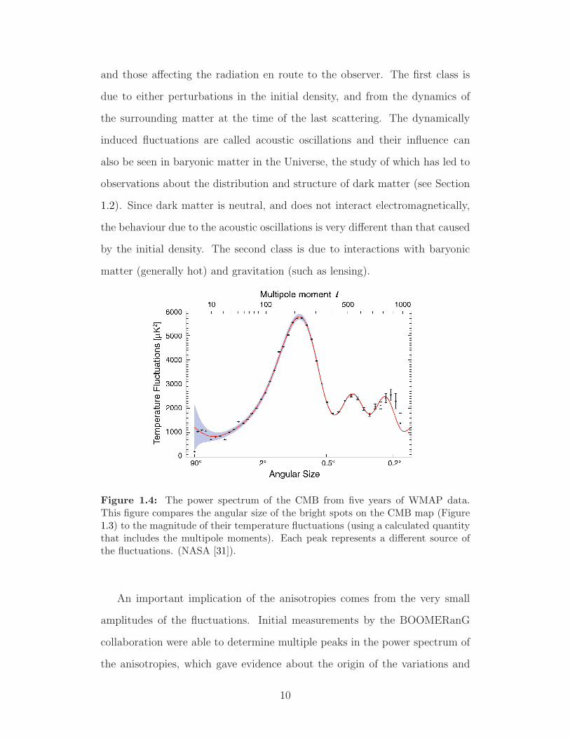
Figure 1.4: The power spectrum of the CMB from five years of WMAP data.This figure compares the angular size of the bright spots on the CMB map (Figure1.3) to the magnitude of their temperature fluctuations (using a calculated quantitythat includes the multipole moments). Each peak represents a different source ofthe fluctuations. (NASA [31]).
An important implication of the anisotropies comes from the very small
amplitudes of the fluctuations. Initial measurements by the BOOMERanG
collaboration were able to determine multiple peaks in the power spectrum of
the anisotropies, which gave evidence about the origin of the variations and
10

magnitude of their contributions. They were able to measure cosmological
constants and found them to be in agreement to a model of an expanding
Universe whose overall shape is flat [32]. However, the small fluctuations
would not be enough to cause the structure formation of the Universe that
we see today, which is a dense network of filaments with great spaces between
them (see Section 1.2). Dark matter would be needed to help produce the
structure formation seen today. The power spectrum of the CMB, as measured
by WMAP, is shown in Figure 1.4. A more in-depth analysis was done by
the WMAP collaboration, which included data from previous experiments,
such as BOOMERanG and COBE, and the Sloan Digital Sky Survey (SDSS).
With detailed information about the CMB they have been able to calculate
the ratios of baryonic matter and dark matter to the total composition of
the Universe required to produce the CMB at the time of the last scattering.
These measurements, along with those performed by other experiments, fit
very well with other observations such as supernovae data and gravitational
lensing. The WMAP team reports [30]:
Ωc = 0.227 ± 0.014 Dark matter density
Ωb = 0.0456 ± 0.0016 Baryon density
ΩΛ = 0.728+0.015−0.016 Dark energy density
which means that there is a far greater abundance of dark matter than visible
matter.
1.1.5 The Bullet Cluster
The Bullet cluster was first detected by the Einstein Observatory, an X-ray
telescope satellite that re-entered Earth’s atmosphere in 1982. The peak in
the Einstein data was re-analysed by a team searching for failed clusters (large
volumes of hot gas that lack galaxies) and optically re-imaged to determine
11

that is was actually a large galaxy cluster with possible gravitational lensing
arcs [33], and designated it 1E 0657-56 in 1995. Follow-up X-ray observations
by the ROSAT and ASCA X-ray telescopes showed that the cluster was un-
usually bright and was likely the result of two merging clusters [34], that such
a hot cluster may challenge current models of the Universe was emphasised.
Using detailed images from HST in 2004 another team was able to produce a
map of the gravitational potential distribution of the clusters using both weak
and strong gravitational lensing. They compared this to X-ray observations
from the Chandra X-ray Observatory, which has much higher capabilities and
resolution than previous studies, and noted a discrepancy in the position of the
luminous baryonic matter compared to the gravitational distribution [35]. The
interpretation of these results was that a smaller cluster passed through the
larger cluster. The collision, at incredibly high speeds, shock compressed the
gas in the clusters, resulting in heating and an unusually high emission of X-
rays. This gas represents the majority of baryonic matter in the clusters, and
was essentially ripped out of the clusters at the site of the collision while galax-
ies and dark matter passed through. The gravity maps show that the mass
distribution, which cannot be accounted for by the galaxies, and the source of
the X-ray emissions are in different places, see Figure 1.5. The Bullet Cluster
data has been touted as direct evidence of non-interacting, non-baryonic cold
dark matter present in galaxy clusters [36, 37].
Even more important is that the difference in mass position peaks and bary-
onic emission peaks is so great that the current theories of modified Newtonian
dynamics (MOND), the most popular alternative to dark matter, cannot ac-
count for the discrepancy. MOND was first proposed by Mordehai Milgrom in
1983 as a solution to the problem presented by the rotation curves of galax-
ies (Section 1.1.2). He proposed that the Keplerian inconsistencies were best
explained by a nonlinearity of Newton’s second law at low accelerations. He
12
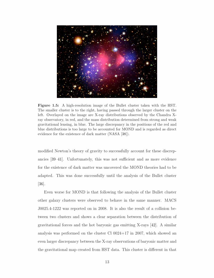
Figure 1.5: A high-resolution image of the Bullet cluster taken with the HST.The smaller cluster is to the right, having passed through the larger cluster on theleft. Overlayed on the image are X-ray distributions observed by the Chandra X-ray observatory, in red, and the mass distribution determined from strong and weakgravitational lensing, in blue. The large discrepancy in the positions of the red andblue distributions is too large to be accounted for MOND and is regarded as directevidence for the existence of dark matter (NASA [38]).
modified Newton’s theory of gravity to successfully account for these discrep-
ancies [39–41]. Unfortunately, this was not sufficient and as more evidence
for the existence of dark matter was uncovered the MOND theories had to be
adapted. This was done successfully until the analysis of the Bullet cluster
[36].
Even worse for MOND is that following the analysis of the Bullet cluster
other galaxy clusters were observed to behave in the same manner. MACS
J0025.4-1222 was reported on in 2008. It is also the result of a collision be-
tween two clusters and shows a clear separation between the distribution of
gravitational forces and the hot baryonic gas emitting X-rays [42]. A similar
analysis was performed on the cluster Cl 0024+17 in 2007, which showed an
even larger discrepancy between the X-ray observations of baryonic matter and
the gravitational map created from HST data. This cluster is different in that
13

the collision occurred more than a billion years ago and, after the dark matter
of both clusters collapsed inward, the kinematic pressures pushed some matter
away from the centre of mass. The observation is of a ring-like structure of
invisible mass surrounding the cluster [43]. The combination of gravitational
lensing data from the high resolution images produced by the HST and other
observations, such as X-rays and microwaves, has become an important tool
in probing the distribution of dark matter, but not only in specific clusters. It
has proven to be the most powerful tool to probe the large scale structure of
the Universe and its relationship to dark matter.
1.2 The Distribution of Dark Matter
Figure 1.6: A portion of the Universe mapped by the SDSS [44]. The void andfilament structure can be clearly seen. The outer edge of the map is two billion lightyears away. The colour scale shows the age of the stars, red being the oldest (SDSS[45]).
14

Several studies have been able to provide a very accurate depiction of the
large scale distribution of dark matter in the Universe. The first clues came
from early redshift studies using faint infrared radiation to catalog large num-
bers of galaxies. These initial observations quickly saw a nonuniform structure
with large voids that were unexpected at the time [46–48]. Several in-depth
studies have been since carried out in the optical and infrared regimes that at-
tempt to gather three dimensional data of the large portions of the sky, avoid
complications arising from our own galaxy, and create the most complete sky
catalogue possible, at the greatest distances. The structure of the Universe
consists of long, inter-connected strings of galaxy clusters connected by fila-
ments of galaxies and gas, with great voids containing negligible amounts of
mass between them, which can be seen in Figure 1.6. Several subsequent large-
scale sky surveys were able to confirm this with increasing resolution and range:
2dFGRS, 2MASS, and 6dFGS [49–51]. The most comprehensive redshift sur-
vey is the ongoing SDSS [44], which produces three dimensional models of the
distribution of galaxies and clusters. The three dimensional power spectrum
of galaxies within the portion of sky mapped by SDSS was able to further
constrain the fraction of baryonic matter in the Universe [52] while a compar-
ison to models ruled out the possibility that the observed filament and void
structure could be created without dark matter [53, 54]. Without cold dark
matter the structure would be washed out and more uniform. Furthermore
models also ruled out the ability for hot dark matter to create these structures
[55] (established earlier using smaller scale redshift surveys).
Further information about the distribution of dark matter within the large
scale structure of the Universe has been developed using contributions from
several data sets. For instance, the COSMOS project, undertaken with the
HST, combines data from several sources, including the Chandra X-Ray Ob-
servatory, the XMM-Newton X-ray telescope, and the Very Large Array radio
15
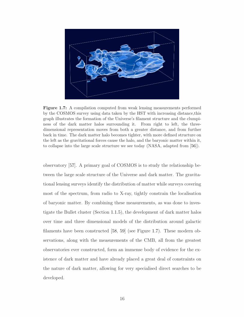
Figure 1.7: A compilation computed from weak lensing measurements performedby the COSMOS survey using data taken by the HST with increasing distance,thisgraph illustrates the formation of the Universe’s filament structure and the clumpi-ness of the dark matter halos surrounding it. From right to left, the three-dimensional representation moves from both a greater distance, and from furtherback in time. The dark matter halo becomes tighter, with more defined structure onthe left as the gravitational forces cause the halo, and the baryonic matter within it,to collapse into the large scale structure we see today (NASA, adapted from [56]).
observatory [57]. A primary goal of COSMOS is to study the relationship be-
tween the large scale structure of the Universe and dark matter. The gravita-
tional lensing surveys identify the distribution of matter while surveys covering
most of the spectrum, from radio to X-ray, tightly constrain the localisation
of baryonic matter. By combining these measurements, as was done to inves-
tigate the Bullet cluster (Section 1.1.5), the development of dark matter halos
over time and three dimensional models of the distribution around galactic
filaments have been constructed [58, 59] (see Figure 1.7). These modern ob-
servations, along with the measurements of the CMB, all from the greatest
observatories ever constructed, form an immense body of evidence for the ex-
istence of dark matter and have already placed a great deal of constraints on
the nature of dark matter, allowing for very specialised direct searches to be
developed.
16

1.3 Candidates for Dark Matter
The body of evidence just presented has given the experimental community
a very good idea of what to look for to confirm the existence of dark matter.
It has also allowed the theoretical community to try to place dark matter
particles within the models of particle physics beyond the Standard Model.
Dark matter does not interact via the strong interaction or electromagnetically;
it is particulate, and does not form larger atoms. It is neutral and massive,
travels slowly enough to be gravitationally bound to stars and galaxies, and is
non-baryonic. There is no known particle with these characteristics, nor are
there any such hypothetical particles predicted by the Standard Model. There
is, however, an entire zoo of particles beyond the standard model that may
be suitable to make up dark matter. Many of these collectively fall under the
generic classification of WIMPs, while another candidate, the axion, is distinct
due to its much lower mass. While we search for a dark matter candidate, it
is accepted that the distribution is partially composed of candidates already
ruled out by observation, such as MACHOs or relativistic neutrinos. For a
more complete review of many more possible dark matter candidates see [60].
1.3.1 WIMPs
Neutralinos
The neutralino is predicted by the leading extensions to the Standard Model:
supersymmetry (SUSY) and the minimal supersymmetric Standard Model
(MSSM), which is a reduction of supersymmetry to produce the fields of the
Standard Model. There are several good candidates for WIMPs in SUSY, but
many are ruled out by observational evidence, such as the gravitino which
would be hot dark matter, or the sneutrino which is unstable and would not
exist in the observed abundance. The best candidate for WIMPs in SUSY is
17

the lightest supersymmetric particle (LSP). A new symmetry is expected in
SUSY, called R-parity for which we assign all the Standard Model particles R
= 1, and all the super-partners R = −1. When SUSY is minimised R-parity
will be conserved, the consequence of which will be that the LSP is stable (see
[61]). In MSSM the LSP is the neutralino, which becomes the best WIMP
candidate. To date no super-partners have been detected in a lab, but with
the completion and commissioning of the LHC at CERN, and first collisions
taking place in 2009, the rise or fall of SUSY is close at hand. Neutralinos are
a leading candidate for two main reasons: they easily conform to the body of
evidence for dark matter, and the SUSY theories, particularly MSSM, are well
understood. MSSM is mathematically robust and calculations of neutralino
densities can be performed.
Lightest Kaluza-Klein Particles
During early searches for unification theories, the Kaluza-Klein (KK) theory
was proposed to unite gravity and electromagnetism using extra dimensions.
This was overtaken by the emergence of the strong and weak interactions,
however. The theory was revisited several times by such theories as string
theory and large extra dimensions. Of particular note are theories with extra
dimensions that are compactified, that is, that allow all particles to propa-
gate through all of the dimensions. Such theories are called universal extra
dimensions and particles have their momentum quantised proportional to R−1,
the size on the extra dimension. The lightest neutral and stable KK particle
(LKP) then makes an excellent candidate for dark matter, falling under the
WIMP classification.
18

Heavy Photons
Under certain theoretical conditions, the breaking of global symmetries may
give rise to pseudo-Goldstone bosons. Such conditions lead to gauge theo-
ries which produce Higgs bosons in which symmetries are not exact and must
be explicitly broken. Where the result would normally be an exact symme-
try, spontaneously broken, and producing a massless Goldstone boson, such
approximate symmetries produce spinless bosons with small masses, so-called
pseudo-Goldstone bosons [62]. In such models the Higgs is a pseudo-Goldstone
boson and is naturally light, while other heavy particles are produced. A new
symmetry can be introduced to create T-parity which forces the lightest par-
ticle with odd T-number to be stable, this particle becomes the candidate
for dark matter [63]. The little Higgs theories are fairly new and still being
adapted, but there is hope that the LHC will be able to probe the parameters
required very quickly and allow for either rapid development (or rapid demise).
1.3.2 Axions
An outstanding problem in physics is why cp-symmetry is violated in elec-
troweak theory but seems to be conserved in quantum chromodynamics, deal-
ing with the strong interaction. A popular solution is Peccei-Quinn theory,
which introduces a new global symmetry that is spontaneously broken. The
resulting Goldstone boson is the axion, given mass from the model’s strong
interaction [64]. Searches for axions have been ongoing, but have only been
able to constrain the mass to < 0.01 eV, which makes it distinct from other
WIMP candidates. The ability to detect axions in this range by dark matter
experiments is close at hand and their parameter space may be ruled out by
the next generation of direct searches. If both SUSY is correct and axions are
discovered, then the LSP is the partner to the axion, the axino, which will
replace the axion as the favourable dark matter candidate.
19

1.4 Detection of WIMP Dark Matter
The nature of WIMPs described above limits the methods that we may use
to search for them. Since WIMPs will have a very low density, and have
been shown to have a small scattering cross section by experiments already
conducted, WIMP scattering events are very rare. Experiments are typically
located deep underground and designed to have very low backgrounds. We
know that WIMPs will only be found by two of the fundamental interactions,
weak and gravitational and we have already observed and studied many of the
gravitational effects (and we are still searching for new evidence).
A confirmation of the existence of dark matter in the proposed particle form
will have to come from the observation of weak effects. The experiments capa-
ble of doing so that have been designed, operated, or proposed are classified as
either direct or indirect. The direct searches are additionally distinguished by
whether they are spin-dependent (SD) or spin-independent (SI), and whether
they are directional. Indirect searches for WIMPs look for the products of their
annihilation from a WIMP encountering its antiparticle, or another WIMP if
they are Majorana particles (they are their own antiparticle). Direct searches
look for evidence of a WIMP scattering off of a target by studying the energy
deposited in the material by the recoiling nucleus which can produce a variety
of effects. There are four primary detectable forms of deposited energy being
currently studied: heat, sound, ionisation, and scintillation light. Ionisation is
detected in conjunction with another form of energy to give more information
about an event.
The dependence on the type of spin coupling is the primary distinction
among experiments. In order to design an effective experiment we calculate
the WIMP detection rate for a given theoretical model (although with approxi-
mations the calculation becomes largely model-independent). The parameters
20

of such calculations are the WIMP mass and the interaction cross section (and
the energy spectrum of annihilation products in the case of indirect detection).
The equation is constructed using the different WIMP-nucleon couplings. In
the non-relativistic limit only two couplings contribute: axial-vector coupling
to nuclear spin (SD), and scalar coupling to the nuclear mass (SI). Note that
SD calculations differ depending on whether the WIMP scattering is due to
neutrons or protons. Both couplings always contribute and should be added
together. However it is assumed, in general, that only one of the couplings
dominates. We have, therefore, two sets of WIMP parameters to probe inde-
pendently. Most experiments are of the SI type and it has been shown that
for heavier target nuclei the mass coupling is dominant for most supersymmet-
ric models. In SD coupling, nucleons with different spin states can cancel in
the overall coupling strength if different, whereas for SI coupling the coupling
strength is dependent on the square of the mass number. The contributions
from SI and SD coupling are model dependent and significantly contribute
to model uncertainty [61]. So far WIMP searches have produced null results,
which are reported as exclusion zones in the parameter space of the WIMP
cross-section and mass within the sensitivity of the experiment. These exclu-
sion plots are distinct for each coupling, and are shown in Figures 1.8 and 1.9
in Section 1.5 for SD and SI (proton and neutron), respectively.
Directional dark matter experiments are sensitive to the direction of the
arrival of the incoming WIMP. Many detectors of this type use time projec-
tion chambers (TPCs) with notable examples being the long running DRIFT
(Boulby mine) experiment and the newly developed DMTPC (WIPP) and
NEWAGE (Kamioka). For a current review on the status of directional dark
matter experiments see [65].
The following sections will outline the indirect search programmes, describe
how the energy deposited in a direct detection experiment is utilised, and
21

briefly outline those scientific programmes. I will provide more detail about
the current experimental limits and the programmes achieving them, including
how the DEAP collaboration will use scintillation light from liquid argon to
detect WIMPs.
1.4.1 Indirect Detection
Many of the extensions to the standard model predict that their lightest sta-
ble particles may annihilate and even predict the product and whether the
LSP should be a Majorana particle. Evidence for WIMP annihilation would
come in the form of gamma rays, neutrinos, anti-protons, or positrons. Some
experiments have already reported excesses of gamma rays, positrons, or anti-
protons originating in deep space, but the sources are not well understood
and other astrophysical explanations (e.g. pulsars) are able to account for
them. Gamma ray results have notably come from the EGRET experiment on
the Compton Gamma Ray Observatory, and the current search from the Fermi
Gamma-ray Space Telescope, launched 2008. Observations of anti-matter have
notably been reported from the PAMELA instrument. For a more complete
review of these deep space observations, their results, and their implications,
see [60].
Due the difficulties associated with deep space indirect dark matter searches
it has been proposed that high density dark matter around a heavy, nearby
object may produce a more distinct signal. There are two experiments cur-
rently operating that search for neutrinos from the centre of the Earth or the
Sun that may be due to WIMP annihilation. ANTARES is a water Cherenkov
detector located in the deep Mediterranean sea. It has a similar counterpart at
the South Pole, the IceCube Neutrino Observatory. Both detectors are similar
in their construction, deploying long strings of detector modules that measure
Cherenkov radiation from natural water using PMTs. They complement one
22

another in their direction and location and both are in the beginning of their
data taking runs [66, 67].
1.4.2 Direct Detection
Historically, development of dark matter detection needs was motivated by
the need to move to higher sensitivity targets, and then to larger scales. The
earliest devices were semiconductor-type, whose scientific goals were primarily
aimed at neutrino physics, followed by solid scintillators. The need for higher
sensitivity, better signal identification, and background rejection led to ad-
vances in cryogenic and multi-phase detectors, such as the XENON and CDMS
collaborations (discussed in Sections 1.5.3 and 1.5.1, respectively) which have
become leaders in the field with small SI detectors. The current push is to
build very large scale experiments, with interest in several different detector
technologies, notably the noble liquid detectors and cryogenic Ge crystals, but
also from newer technologies, such as innovative bubble chambers.
Heat depositions are measured as thermal phonons using cryogenic bolome-
ters. There have been several experiments using this method: EDELWEISS
(LSM) and CDMS (Soudan), which also measure ionisation; and CRESST
(LNGS) and ROSEBUD (LSC), which also measure scintillation light. EDEL-
WEISS [68] and CDMS both use high-purity Ge crystals, while ROSEBUD
used sapphire (Al2O3) [69], and CRESST used CaWO4 [70]. CDMS has made
one of the most sensitive measurements to date, while CRESST, ROSEBUD,
and EDELWEISS have made plans to form a larger collaboration, EURECA
(LSM), which will create a tonne scale cryogenic detector looking for both
thermal phonons and scintillation light [71]. A description of the CDMS ex-
periment, its current results and future goals will be discussed in section 1.5.1.
A novel approach to dark matter detection uses superheated liquids to
make a bubble chamber. The PICASSO (SNOLAB) experiment measures the
23
acoustic phonons created by phase changes in the target liquid. The PICASSO
experiment is of the SD type and has demonstrated very strong discrimination
power at different temperatures. It has recently set the current limit for SD-
proton parameter space and its results will be discussed in Section 1.5.2. Two
similar experiments are COUPP and SIMPLE, both SD. SIMPLE (LSBB)
uses several superheated droplet detectors containing C2ClF5 in a gel. When
energy is deposited in the detectors, the gel undergoes a phase transition to gas
and the pressure change and acoustic signatures are recorded [72]. COUPP
(Fermilab) is a more conventional bubble chamber with a superheated CF3I
target. Events are recorded with a camera and the shape and rate of bubble
development is used to discriminate event sources [73].
The scintillation based detectors make up the majority of the dark matter
experimental development. Early experiments used solid scintillators, such as
NAIAD (Boulby [74]) and DAMA (LNGS, see Section 1.5.4), which deployed
NaI detectors. More recently, KIMS (Yangyang [75]) used CsI(Tl) crystals to
achieve higher sensitivity. All three experiments are sensitive to both SI and
SD coupling, but were shown to be the most competitive in the SD regime
for proton coupling. The SI and SD-neutron sectors have been dominated by
CDMS and the noble liquid scintillation experiments. The competitive field of
direct dark matter detection is largely at the same stage: many collaborations
have built prototype detectors to test the projected sensitivity and background
rejection power of their design, some have built intermediate sizes that are
currently operational, and most plan to enter the tonne-scale regime in the
near future. Targets are almost exclusively liquid argon or xenon, LXe being
most popular, and they are either single phase, or two phase, incorporating a
TPC and using a ratio of scintillation light to ionisation as a form of pulse-
shape discrimination (PSD).
The Cryogenic Low Energy Astrophysics with Noble gases (CLEAN) is a
24

medium-sized, single-phase detector at SNOLAB that was developed alongside
DEAP. It will be run interchangeably with both argon and neon to be able
to compare WIMP signals from both targets [76, 77]. Testing was performed
with a small prototype and a scaled up version with 500 kg of active mass
is under construction at SNOLAB. Another single-phase detector is XMASS
at Kamioka Underground Observatory. XMASS will use an 800 kg LXe tar-
get surrounded by an array of 642 small, hexagonal PMTs [78]. Including
DEAP, there are only three single-phase detectors in development, with the
DEAP programme poised to become the first to reach the tonne scale. The
operational principles of all three detectors are very similar, while the engi-
neering tasks and designs differ greatly, a primary objective of which is having
ultra-low backgrounds. The PSD techniques developed by the DEAP/CLEAN
collaboration sets them apart from the XMASS programme.
There have been several two-phase detectors built and under construction.
These detectors allow for a region of gas above the liquid. This gas region
forms the end of a TPC while the liquid is used as a drift chamber. When
an event occurs in the liquid phase, scintillation is produced and measured
while ionisation electrons are drifted into the gas phase, where additional scin-
tillation light is generated. The ionisation may also be counted directly with
proportional counters. Using argon as a target are WArP (LNGS) and ArDM
(CERN, surface). The WArP collaboration has recently completed a detector
with 140 kg active mass and has begun taking data underground [79] while
ArDM is developing a much larger detector at surface with an 850 kg active
mass [80], with future plans to move underground (unspecified site). Among
the xenon based two-phase experiments, two groups were able to build pro-
totype detectors and set competitive constraints on WIMP parameter space:
XENON10 (LNGS) and ZEPLIN-III (Boulby). The XENON collaboration,
along with CDMS, has been able to build the most sensitive detectors to date
25

and will be discussed in Section 1.5.3.
1.4.3 Producing WIMPs at Accelerator Labs
An additional way in which WIMP candidates may be discovered is their pro-
duction in the most powerful particle accelerators: the Tevatron at the Fermi
National Accelerator Laboratory and the Large Hadron Collider at CERN.
These colliders produce the most energetic particles in a laboratory setting to
date and may be able to detect WIMP candidates as missing energy from a
collision. The LHC in particular will be able to probe most of the parame-
ter space needed for many supersymmetric scenarios. Such constraints placed
on extensions to the standard model and the confirmation of the existence of
other particles within these theories will allow dark matter searches to narrow
the parameter space of their search and complement the finding by narrow-
ing down the range of possible WIMP candidates. Unfortunately, detecting
WIMP candidates produced in particle accelerators will not be enough to
prove the existence of dark matter. A confirmation that the discovered parti-
cles are actually abundant in the Universe with required distributions will still
be needed.
1.5 Current Dark Matter Searches
In the SI regime, the best limits on the interaction cross section and mass for
a WIMP have been set by the XENON and CDMS collaborations, followed
by ZEPLIN and EDELWEISS. The current limits for SI cross sections as a
function of WIMP mass are shown in Figure 1.8. These same groups (ex-
cept EDELWEISS) also dominate the SD-neutron regime, with the XENON
and ZEPLIN groups achieving the highest sensitivity, Figure 1.9 (top). The
SD-proton regime is dominated by solid scintillator experiments and bubble
chambers, led by PICASSO and COUPP, especially for low WIMP mass, fol-
26

lowed by older results from KIMS and NAIAD, Figure 1.9 (bottom). The
following sections will give details about the leading experiments using each
of the primary methods for direct detection.
WIMP Mass [GeV/c2]
Cro
ss−
sect
ion
[cm2 ] (
norm
alis
ed to
nuc
leon
)
101
102
10310
−44
10−43
10−42
10−41
10−40
Figure 1.8: Current results from leading WIMP searches for SI WIMP-nucleonscattering. The region above an experiment’s line is the parameter space excludedby that search. The shaded area is the parameter space allowed by DAMA, nowmostly excluded by other experiments. Plot generated using [81] using data from[68, 82–86].
1.5.1 CDMS
The Cryogenic Dark Matter Search (CDMS) uses a combination of ultra-
pure Si (100 g) and Ge (250 g) crystals mounted with photolithographically-
fabricated thin films. These detectors operate at T< 40 mK and the thin films
are able to detect phonons produced by variations from the operating tempera-
ture, with their signals being read by SQUID devices. Detectors are organised
in a tower structure, sitting in a vertical stack. The entire assembly sits in
27

WIMP Mass [GeV/c2]
Cro
ss−
sect
ion
[cm2 ] (
norm
alis
ed to
nuc
leon
)
101
102
10310
−40
10−38
10−36
10−34
WIMP Mass [GeV/c2]
Cro
ss−
sect
ion
[cm2 ] (
norm
alis
ed to
nuc
leon
)
101
102
10310
−38
10−37
10−36
10−35
10−34
Figure 1.9: Current results from leading WIMP searches for spin-dependentWIMP-neutron (top) and WIMP-proton (bottom) scattering. The region abovean experiment’s line is the parameter space excluded by that search. The shadedarea is the parameter space allowed by DAMA. Plots are generated using [81] withSD-neutron data from [82, 87–89], and SD-proton data from [73, 75, 82, 87–91].
28

an electric field, the lowest detector forming the ground reference point. The
electric field drifts ionisation electrons to a warmer stage of the cryostat where
FETs are used to measure the amount of ionisation. The cryostat assembly is
made of high purity copper to ensure low radioactivity, and is shielded with
lead recovered from the ballast of a sunken eighteenth century French ship,
which ensures that radioactive impurities have decayed away sufficiently. The
lead is supplemented with a polyethylene shield to further attenuate neutrons
and the entire cryostat is surrounded by an active muon veto system. Further
shielding has been provided by installing the cryostat in the Soudan Under-
ground Laboratory in northern Minnesota (experimental details from [87, 92]).
Studies of the ratio of phonon signals to the amount of ionisation allow for
precise particle identification, easily vetoing β events while allowing nuclear
recoils. The major experimental hurdles are similar to those of DEAP, prop-
erly identifying neutrons that produce a similar signal to WIMPs, and further
reducing background sources.
The first iteration of the CDMS experiment was CDMS I, during which a
small number of detectors were developed to test multiple new technologies.
They were deployed at a shallow depth of 10.6 m in the Stanford Underground
Facility and later moved to Soudan in 2003. The first WIMP search was taken
with CDMS II beginning in 2006 at Soudan. 30 improved detectors were
deployed in five towers, totalling 4.75 kg Ge and 1.1 kg Si, and run in stages
until 2009. The combined data places the most sensitive restriction on SI
WIMP scattering at high WIMP masses to date [83, 93]. The next phase
is SuperCDMS, in which the detector towers will be replaced with “super”
towers using larger crystals and improved phonon detectors. SuperTower 1
has been installed and features five 1” thick Ge crystals weighing 0.64 kg each.
CDMS plans to achieve a 15 kg Ge detector at Soudan, with future goals to
build a 100 kg Ge detector at SNOLAB (which offers greater shielding than
29

Soudan due to its depth). A major issue facing the CDMS collaboration is the
high cost of manufacturing the Ge detectors compared to PICASSO, COUPP,
and the noble liquid experiments. Achieving a tonne scale detector with noble
liquids will be a fraction of the cost of doing the same with Ge crystals.
1.5.2 PICASSO
The Project in Canada to Search for Supersymmetric Objects (PICASSO)
is located at SNOLAB and uses superheated droplets of C4F10 suspended in
water-based polymerised gel. The droplets are between 10 and 200 µm and
contain the isotope 19F, which is favourable for SD WIMP sensitivity [94].
When the 19F is energised by incident particles it causes its host droplet to
undergo a phase transition to gas which is explosive enough to create measur-
able acoustic signals. PICASSO uses piezoelectric transducers to detect sound
waves caused by these interactions and has demonstrated that the sensitiv-
ity to different sources is dependent on the temperature of the superheated
droplets, which allows their WIMP search to be insensitive to many forms
of background radiation, such as γ and β particles [95]. Each event in the
detectors results in a loss of active volume due to the phase change, which
affects the WIMP sensitivity of a run over time. At the end of a timed run
the detectors are pressurised to return the gas bubbles to liquid droplet form.
The PICASSO experiment has also been run in phases, starting with pro-
totype detectors tested on the surface and underground at SNOLAB and the
Windsor Salt Mine. These were polyethylene containers with only two piezo-
electric transducers filled with 1 L of the polymerised gel containing C4F10.
The droplets at this stage were small, ≈ 11 µm [94]. Advanced detectors be-
gan being installed at SNOLAB in 2007, beginning with a set of four that have
since been running continuously. The goal was to install an array of 32 detec-
tors in independent groups of four, and was completed in 2008. The WIMP
30

search with the full 32 detectors ran through 2009 and culminated in the most
sensitive SD WIMP search to date [91], and continues to collect data. The
new detectors contain 4.5 L of active gel, are made with acrylic containers in
a stainless steel frame, and have nine piezoelectric transducers each.
1.5.3 XENON
The XENON collaboration has developed the leading two-phase noble liquid
dark matter search using scalable technology in a multi-stage programme. The
first iteration, XENON10, used a 15 kg cylindrical LXe target. The cylinder
is constructed with copper rings to provide an electric field, separated with
Teflon spacers. LXe is not contained by the cylinder and PMTs on the outside
use the remaining LXe as an active shield, relying on the excellent stopping
power of the large xenon nuclei. The bottom end is fitted with a quartz
window and an array of 1” square PMTs. The upper end was fitted with a
multi-wire proportional counter finishing the TPC and topped with a second
PMT array within a gaseous xenon stage. Electrons exit the TPC into the
gaseous xenon and scintillate again. The ratio and time difference between the
primary and secondary scintillation light is the basis for particle identification.
The detector is built with copper and stainless steel and shielded inside a castle
made of a layer of depleted lead and polyethylene walls [96]. XENON10 was
deployed underground in the Gran Sasso National Laboratory (LNGS) in Italy
in 2006 and run until 2007, resulting in a WIMP search that remains one of
the most sensitive [84, 97]. The second iteration is XENON100, built in 2008
at LNGS, which began its WIMP search in 2010, with results from 11.2 days
announced [85]. This detector’s design is a scaled version of the prototype with
additional shielding and an active muon veto. XENON100 is claimed to have
the lowest backgrounds of any dark matter experiment currently operating
underground. Again, properly identifying nuclear recoils from neutrons and
31

reducing background sources are ongoing goals of the collaboration. The next
planned upgrade is a one tonne LXe mass immersed in a large water shield
with active muon veto capability.
1.5.4 Controversial Results: DAMA, CoGeNT and
XENON100
There are a few prominent dark matter experiments from the past and present
that I have not commented on that may prove to be very significant. I have
not discussed them due to the controversies resulting from their claims. The
primary concern is that the experimental results from detectors made with
different materials have not always been reconcilable with one another. As
the next generation of detectors comes online, more results are collected, and
careful analysis is performed the controversies should be laid to rest over time.
First is the DAMA collaboration which deployed NaI scintillators at LNGS.
They reported an annual modulation in their signal, but only at very low
energies [98]. This is, significantly, the first claim of seeing a dark matter
signal. There are two problems with the DAMA result: they have not been
able to convince many members of the dark matter community that they
fully understand their backgrounds, and the parameter space in which their
experiment is sensitive has been ruled out with null results by several other
experiments, including the CDMS, XENON100 and PICASSO experiments.
Similar experiments using NaI crystals and lower backgrounds need to be
performed to investigate the signal modulation, preferably in the southern
hemisphere to test whether any observed oscillations are seasonal. Further
probes of the low-mass WIMP region are needed.
The CoGeNT and XENON100 results are very recent, pre-published in
2010 and come directly to odds with one another. CoGeNT (Soudan) uses p-
type point contact (PPC) germanium detectors, it is a small experiment devel-
32

oping the PPC technology for larger application. Their result showed a number
of signals from low energy recoils consistent with low-mass WIMPs, but oth-
erwise unexplained by backgrounds [99]. The first results from XENON100,
released only months later, directly challenge the CoGeNT result by claiming a
null result in the low-mass parameter space to which CoGeNT and DAMA are
sensitive [85]. Furthermore, the XENON100 report has been openly criticised
by both theorists and experimentalists alike [100, 101]. As with the DAMA
result, time should resolve the controversy.
33

Chapter 2
The DEAP Programme
The DEAP programme is divided into two stages: DEAP-1 and DEAP-3600.
The prior is a small prototype currently underground at SNOLAB, while
DEAP-3600 will be a tonne-scale, spherical variant intended for a long term
WIMP search. The prototype was developed primarily to demonstrate pulse-
shape discrimination, and has been used extensively to test and improve anal-
ysis algorithms, and to study and understand the sources of background radia-
tion that we will face when operating DEAP-3600. DEAP-1 has gone through
several operational periods, beginning with a surface run at Queen’s Univer-
sity in Kingston, and the fourth operational period has been running through
August 2010. Many lessons about backgrounds originating in the detector
have been learned and improvements to the construction methods, analysis,
and argon purification system were made. The electronics and PMTs have
been upgraded to match those that DEAP-3600 will use. This has allowed the
analysis code to be adapted to work with these components, while the new
signals are understood in advance of the large detector’s operation.
2.1 DEAP-1
DEAP-1 is a small prototype detector containing 7 kg of LAr in a cylindrical
volume. The chamber is made of a 14” thick acrylic sleeve with TPB deposited
34

in the inside and a reflective coating on the outside. The first two chambers
used TiO2 paint, but the paint was found to be a strong background source and
was subsequently replaced with a TPFE sleeve. The sleeve sits in a stainless
steel tube fitted with glass windows at either end. The glass windows are also
coated with TPB. To ensure low backgrounds from detector materials, a new
acrylic chamber has been made for each operational period, with an evolving
construction process. The dimensions vary, but the chamber is approximately
28 cm long and 14 cm wide, while the windows are 1 cm thick. Acrylic light
guides (20.8 cm long, 14.8 cm wide during the period I studied DEAP-1 data)
separate the PMTs from the glass windows. They are used for two reasons; to
keep the PMTs from cooling to near cryogenic temperatures, and to help block
background neutron radiation. The LAr vessel is housed in a larger stainless
steel shell that provides an insulating vacuum, with the light guides and PMTs
protruding. A schematic of the detector is shown in Figure 2.1.
The process systems are housed above the detector. The LAr is in a closed
system and is liquefied by circulating it through a liquid nitrogen bath. The
nitrogen system is not closed and boils off over time. The liquid level of the
bath is monitored and nitrogen is refilled as needed. The LAr is 99.999%
pure natural argon gas, and initially liquefied in DEAP-1. Impurities from
other atmospheric gases, such as oxygen and nitrogen, can absorb scintillation
light [102, 103], so the LAr is passed through a SAES getter which reduces
impurity concentrations down to less than 0.1 ppb by mass. Additionally a
radon trap is installed to remove radon contamination using activated charcoal.
The experiment is housed in a steel rack which supports the detector, process
systems, and shielding. The LAr chamber is completely surrounded by a water
shield comprised of 20 L water containers (cube-shaped boxes). The gaps are
filled with plastic boards.
35

Figure 2.1: A schematic of DEAP-1. Shown is the LAr chamber, external vacuumchamber, light guides, PMTs, and process systems connections.
2.2 Detecting Dark Matter with Liquid Argon
2.2.1 Scintillation from Noble Gases
Scintillation light is produced in certain materials when ionising radiation in-
teracts with electrons or nuclei within it. Electron recoils are dominant since
the energy delivered to an electron in a collision is inversely proportional to
mass (p2/2m), and the Coulomb attraction being greater for a nucleon. There-
fore, an incoming particle’s energy is less readily absorbed by electron collisions
than those with nucleons, allowing for the rate of electromagnetic events to
be up to several orders of magnitude greater than the rate of nuclear recoils,
due to the great disparity between their masses1. The incoming radiation may
excite or ionise the atoms in the scintillating material when passing through,
and it may have collisions with electrons or nuclei. When the electrons or
nuclei are struck by the incident radiation they recoil through the material
and cause others atoms to ionise or become excited.
1The mass of protons and neutrons is around 940 MeV, compared to 0.5 MeV for anelectron.
36

Energy deposited in the noble gases causes excited atoms to form dimer
pairs (excimers). The excimers are metastable and recombine into stable states
with the release of vacuum ultraviolet (VUV) scintillation light [104]. There
are two mechanisms through which this occurs. The first is direct excitation,
in which an atom is excited and bonds to an un-excited atom (illustrated with
argon):
Ar∗ + Ar → Ar∗2
Ar∗2 → 2Ar + hν(2.1)
The second process is through ionisation, where an ion bonds to another atom
and de-excites into a dimer before recombination produces a scintillation pho-
ton:
Ar+ + Ar → Ar+2
Ar+2 + e− → Ar∗∗ + Ar
Ar∗∗ → Ar∗ + heat
Ar∗ + Ar → Ar∗2
Ar∗2 → 2Ar + hν
(2.2)
In Equations 2.1 and 2.2 the term hν represents the scintillation photon and
the process Ar∗∗ → Ar∗+heat is non-radiative. Each ionised and excited atom
from the incident radiation produces one VUV photon, unless the excimers are
destroyed by another process (Section 2.3.1). In the case of noble liquids, these
VUV photons do not have enough energy to excite a ground state atom and
so the scintillation light is not re-absorbed by the liquid.
The excimer Ar∗2 was observed to undergo recombination in distinct slow
and fast components [105]. The Ar∗2 forms one of two distinct states: a singlet,
1Σ+u , and a triplet, 3Σ+
u . It has been shown that the mechanism of energy
deposition (linear energy transfer) affects the ratio of 1Σ+u and 3Σ+
u states
produced. Excitation from β and γ particles produce many more excimers
37
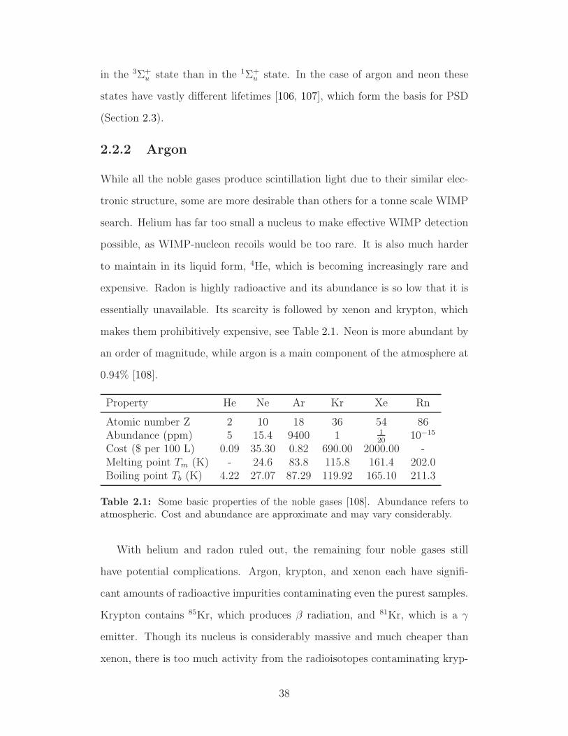
in the 3Σ+u state than in the 1Σ+
u state. In the case of argon and neon these
states have vastly different lifetimes [106, 107], which form the basis for PSD
(Section 2.3).
2.2.2 Argon
While all the noble gases produce scintillation light due to their similar elec-
tronic structure, some are more desirable than others for a tonne scale WIMP
search. Helium has far too small a nucleus to make effective WIMP detection
possible, as WIMP-nucleon recoils would be too rare. It is also much harder
to maintain in its liquid form, 4He, which is becoming increasingly rare and
expensive. Radon is highly radioactive and its abundance is so low that it is
essentially unavailable. Its scarcity is followed by xenon and krypton, which
makes them prohibitively expensive, see Table 2.1. Neon is more abundant by
an order of magnitude, while argon is a main component of the atmosphere at
0.94% [108].
Property He Ne Ar Kr Xe Rn
Atomic number Z 2 10 18 36 54 86Abundance (ppm) 5 15.4 9400 1 1
2010−15
Cost ($ per 100 L) 0.09 35.30 0.82 690.00 2000.00 -Melting point Tm (K) - 24.6 83.8 115.8 161.4 202.0Boiling point Tb (K) 4.22 27.07 87.29 119.92 165.10 211.3
Table 2.1: Some basic properties of the noble gases [108]. Abundance refers toatmospheric. Cost and abundance are approximate and may vary considerably.
With helium and radon ruled out, the remaining four noble gases still
have potential complications. Argon, krypton, and xenon each have signifi-
cant amounts of radioactive impurities contaminating even the purest samples.
Krypton contains 85Kr, which produces β radiation, and 81Kr, which is a γ
emitter. Though its nucleus is considerably massive and much cheaper than
xenon, there is too much activity from the radioisotopes contaminating kryp-
38

ton to make it a suitable candidate for a tonne-scale WIMP search. The lower
activity and larger nucleus2 of xenon offset its higher cost. Xenon is found
containing 85Kr while argon contains significant amounts of 39Ar, a γ emitter
produced by atmospheric cosmic ray reactions. Neon does not have any natu-
rally occurring long-lived radioisotopes, but has a very small cross section due
its much smaller nucleus, which makes it unfavourable for a high-sensitivity
WIMP search. However, since it can be made very pure, it has a much better
chance of probing the low-mass WIMP sector, which is much harder to obtain
with argon and xenon due to their high β and γ activity.
Property Ne Ar Kr Xe
λ (nm) 77 128 147 1741Σ+
u time (ns) 18.2 ± 0.2 7.0 ± 1.0 2.1 ± 0.3 4.3 ± 0.63Σ+
u time 14.9 ± 0.3 µs 1.6 ± 0.1 µs 80 ± 3 ns 22.0 ± 0.2 nsScintillation yield 1.5 4.0 - 4.2(×104 photons/MeV)
Table 2.2: Summary of scintillation properties for the primary choices of nobleliquids [107, 109–112]. λ is the wavelength of scintillation light produced. 1Σ+
u timeand 3Σ+
u time are the length of time it takes for recombination from each state.
The next most important factors for choosing Ar as our target are the prop-
erties of the scintillation produced. Primarily, these are the amount of light
produced, the difference between recombination of the 1Σ+u and 3Σ+
u states (for
single-phase detectors), and the amount of ionisation produced (for TPC-type
detectors). Krypton and xenon have a very small difference between the 1Σ+u
and 3Σ+u recombination times, which makes them unsuitable for a single-phase
experiment since PSD would not be able to achieve levels required for a com-
petitive WIMP search. Table 2.2 contains a summary of scintillation light
yields and recombination times for neon, argon, krypton, and xenon in their
2It should be noted that the common stable isotopes of xenon have between 74 and 80neutrons which is comparable to the total mass number of krypton’s common stable isotopes(between 80 and 86).
39

liquid phases.
Thus, Xe and Ar are the best choices for a large scale and competitive
WIMP search, while argon is a better choice for single-phase experiments
since PSD can be done without the need for a TPC. It is also desirable due its
low cost and great abundance. Contamination by 39Ar does present a problem
and will be discussed in Section 3.0.2. Both the LXe and LAr programmes
have been developing purification techniques to remove the isotopes.
2.3 Pulse-shape Discrimination and Analysis
As shown in Table 2.2, the difference between recombination times for Ar∗2 in
the 1Σ+u and 3Σ+
u states is large enough to perform accurate PSD. The ratio of
1Σ+u and 3Σ+
u states has been measured for argon and accurate discrimination
between nuclear recoils and electromagnetic events has been demonstrated
by the DEAP/CLEAN collaboration [77, 111]. In DEAP-1, we are able to
distinguish events by studying the ratio of prompt light from an event to
the event’s total light. Thus ratio is called Fprompt. A large fraction of late
light from γ and β interactions distinguishes them from nuclear recoils due to
neutrons, αs and WIMPs. Example waveforms for both types of events with
the regions of prompt and late light highlighted are shown in Figure 2.2.
We use the Fprompt ratio as an observable after defining the prompt and late
regions of light. The leading edge3 is the time when the waveform first crosses
a threshold of 5 mV (about 110
the pulse height due to a single photoelectron),
denoted by tA and tB. The prompt region is 150 ns wide, beginning from 50 ns
before the leading edge. The amount of light in each region is calculated by
integrating the waveform after making baseline corrections: Q =∫
V(t) dt.
The charge Q is converted to units of photoelectrons (pe) using a calibration
3Code variables Edge0 and Edge1 for each PMT.
40

s)µTime (0 1 2 3 4 5 6 7 8 9 10
Pul
se a
mpl
itude
(V
)
)γ, β event (prompt
Sample pulse of a low F
s)µTime (0 1 2 3 4 5 6 7 8 9 10
Pul
se a
mpl
itude
(V
)
Late light regionBlue: Prompt light regionYellow:
)α event (WIMP, n, prompt
Sample pulse of a high F
Figure 2.2: waveforms from two events in DEAP-1. The left shows an event withlow Fprompt, from a β or γ particle. The right shows a high-Fprompt event froma nuclear recoil (neutron calibration). The regions of prompt and late light arehighlighted.
factor C. We have:
Fprompt ≡∫ tA+100ns
tA−50nsCAVA(t) dt +
∫ tB+100ns
tB−50nsCBVB(t) dt
TotalPE(2.3)
where the scripts A and B refer to each of the two PMTs in DEAP-1 and
TotalPE is the total light in the pulse, defined as:
TotalPE ≡∫ 10µs−(tA−50ns)
tA−50ns
CAVA(t) dt +
∫ 10µs−(tB−50ns)
tB−50ns
CBVB(t) dt (2.4)
CA and CB are determined iteratively while taking data and the range is from
50 ns before the leading edges to the end of the waveform. 4 µs of the tail
of waveforms with TotalPE < 200 pe is scanned for pulses crossing a 5 mV
threshold. These pulses are integrated over a 25 ns window and the integrals
are histogrammed for each run. The mean is determined to be the average
charge due to single photoelectrons (SPE) in each PMT, CA and CB. Figure
2.3 shows these calibration plots for a typical run. The above definitions are
specific to the way the data used in this thesis was analysed. The definition
of Fprompt can, and should, be generalised. For instance, the current iteration
of DEAP-1 uses different integration ranges and new software algorithms are
41

being developed that attempt to count SPE, thus Fprompt would not be defined
using integrals.
The region of interest in TotalPE for WIMP activity is between 120-240 pe,
or about 40-80 keVee4. We combine this by limiting Fprompt to < 0.7 to form
a region in which PSD studies focus, a primary goal of DEAP-1 being to
demonstrate that the number of electromagnetic events from γs in this region
is small. Figure 2.4 shows the distribution of events in Fprompt–TotalPE param-
eter space from 22Na PSD runs taken during the 2007 surface run (described
in Section 2.4). Note that the Fprompt space occupied by γ events smears out
at low energy, this is because the ratio of 1Σ+u and 3Σ+
u states produced by
nuclear and electromagnetic events varies with energy [113].
SPE charge (pC)-1 0 1 2 3 4 5
Cou
nts
(arb
itrar
y un
its)
0
0.2
0.4
0.6
0.8
1
1.2
1.4
PMT A
PMT B
Figure 2.3: The SPE charge spectra for each DEAP-1 PMT from a typical run.The mean is iteratively determined and used to determine the absolute light yieldand to calibrate calculations of pulse charge to number of pe [113].
When not taking background data (or performing a WIMP search in the
case of DEAP-3600) there are three modes of operation in DEAP-1 that de-
termine analysis parameters and PSD quality. A neutron source is used to
4Electron-equivalent energy, see Section 2.3.1
42

Number of photoelectrons0 50 100 150 200 250 300
prom
ptF
00.10.20.30.40.50.60.70.80.9
1
Figure 2.4: Fprompt verses TotalPE distribution for triple-coincidence γ eventsfrom an 22Na source. The data here is from the 2007 surface run and used todetermine PSD capabilities [113].
determine the detector response to nuclear recoils, and an 22Na source is used
for energy calibration and PSD analysis.
2.3.1 Scintillation Efficiency
There is a discrepancy between the light yield of nuclear and electromagnetic
events. The ratio between the amount of light produced by the two types of
event, given that they have the same initial energy, is called the nuclear recoil
scintillation efficiency, Leff. We use an 22Na source for energy calibration
which is a γ emitter, so the value we determine is specific to the light yield
from electromagnetic events, expressed in keVee, electron-equivalent energy.
To determine the energy of high-Fprompt, nuclear recoil events we use the Leff:
E[keVee] = E[keVr] × Leff
where keVr is the nuclear recoil energy. The energy threshold for WIMP
scattering is set by a detector’s PSD and the detector material’s Leff. The
mechanisms that cause different ratios of 1Σ+u and 3Σ+
u states, and different
43

light yields for electronic and nuclear recoils are not fully understood. However,
a major factor that contributes to the lower scintillation efficiency of nuclear
recoils is quenching, which are processes by which a photon is not produced
after a nuclear recoil event. Lindhard quenching is a process where heat is
produced instead of the creation of excimers. Another form of quenching is
through biexcitonic collisions:
Ar∗ + Ar∗ → Ar + Ar+ + e−
where the result is that two excitons are required to produce a single photon
(from the resulting Ar+).
The LAr Leff for neutrons with different energies has been measured by the
CLEAN collaboration using a deuterium-deuterium neutron generator. They
measured the Leff for a range of neutron energies from 10-250 keVr and found
a mean value of 0.25 ± 0.02 for recoils above 20 keVr [114]. The results are
shown in Figure 2.5. Other measurements of much higher energy α particles
found a Leff for them to be 0.72 ± 0.04 [115, 116].
Energy (keVr)0 50 100 150 200 250
eff
L
0
0.05
0.1
0.15
0.2
0.25
0.3
0.35
0.4
0.45
0.5micro-CLEAN
WARP
0.02 +0.01±Mean 0.25
Figure 2.5: Leff as a function of recoil energy. The cause of the upturn below20 keVr is not known, and the red line is the weighted mean for events above20 keVr [114]. Included is a measurement made by the WArP collaboration [117].
44

2.3.2 22Na Calibration
511 keV γ rays were produced by an 22Na source for energy calibration and
PSD studies. To reduce the background rate while operating on the surface,
two NaI detectors were used to trigger the 22Na γ events. The first is a PMT
behind the source to collect γ rays travelling backwards relative to DEAP-
1, and the second is an annulus-shaped NaI detector surrounding the source
that detects additionally produced 1274 keV γ rays. The two trigger detectors
combine with DEAP-1 to form a triple-coincidence γ tag. Due to shielding
provided by SNOLAB, when DEAP-1 was moved underground a single PMT
was used for tagging the 511 keV γ ray from the 22Na source, providing a
double-coincidence tag. The calibration varies over time, but is approximately
2.8 pe/keVee.
2.3.3 PSD Studies
We quantify the level of PSD, or discrimination power, at a given energy as
the probability of counting an electromagnetic event as a nuclear recoil in the
region of interest. To determine the quality of PSD, 22Na data is taken with
the addition of another trigger from a single-channel analyser (SCA). This cuts
the majority of events which have energies well above the region of interest
(120-240 pe). The cut decreases dead time and allows more events in the
region of interest to be collected in a shorter time. The PSD quality is checked
by selecting all good events (see Section 2.3.4) that pass the coincidence cuts
and studying the Fprompt results. Additionally, neutron calibration data has
been used. The PSD is accurate if tagged electromagnetic events from the
511 keV γ rays do not impinge on the Fprompt region occupied by tagged neutron
events from calibration. While the detector was operated on the surface 63
million triple-coincidence events were collected. Only 16.7 million survived the
data cleaning cuts and had energies within the region of interest. None had
45

Fprompt > 0.7, resulting in a demonstrated discrimination power of 6.8 × 10⁻⁸
[113]. The results of the surface run are shown in Figure 2.6, which includes
tagged neutron events. Once DEAP-1 was moved to SNOLAB a primary goal
was to build a large dataset to study the PSD level. By the end of the first
two underground runs the PSD level was pushed down to 9.26 − 9.46 × 10⁻⁹
[118, 119].
promptF0 0.1 0.2 0.3 0.4 0.5 0.6 0.7 0.8 0.9 1
Eve
nts/
0.01
wid
e bi
n
1
10
210
310
410
510
610-ray eventsγ 7 10×1.7
100 nuclear recoil events
Figure 2.6: Fprompt distribution of PSD events from the surface run. There are noelectromagnetic events in the nuclear recoil region.
2.3.4 Additional Variables and Data Cuts
This section introduces additional variables that are used in later analysis.
The primary variables I used in my background studies are Fprompt, TotalPE,
and Zfit. The Zfit variable is an approximate measure of an event’s position,
based on the amount of light collected by each PMT. We can use this variable
to restrict events to those occurring in the LAr volume. Zfit is calculated as:
Zfit ≡ 35.2 cm×∫ 10µs−(tA−50ns)
tA−50nsCAVA(t) dt−
∫ 10µs−(tB−50ns)
tB−50nsCBVB(t) dt
TotalPE(2.5)
where 35.2 cm is the distance from the middle of the LAr volume to the faces of
the PMTs. This variable acts differently during each period due to changes in
46
the detector surfaces and light guides. When DEAP-1 was first underground
the Zfit position of background events was centred around 5 or 6 cm with more
light coming from the detector centre than the ends. Optical effects due to
the change in reflectivity were observed when the TPFE sleeve was used in
place of the TiO2 paint. A Zfit calibration was undertaken showing a strong
correlation between Zfit = 0 and event positions in the detector centre. It
also showed that position reconstruction degraded at Zfit = ± 10 cm, which
is near the light guides. However, a dependence on light yield and Zfit was
found, which must be corrected during analysis.
Additional variables are used for the data cleaning cuts listed in Appendix
A. These cuts remove “bad” events, which may have strange pulse shapes. The
variables PreSignal0 and PreSignal1 ensure that there are no pulses before the
prompt light. PmtCutID0 and PmtCutID1 prevent waveforms with multiple
signals (pile-up) from being selected. The primary cut is on timing, ensuring
that the prompt pulses in both waveforms occur within 20 ns of each other and
within 30 ns of the mean prompt pulse time. This is done using the trigger
time mentioned in Section 2.3, Edge0 and Edge1.
2.4 Detector Operations
The DEAP-1 detector is currently in its fourth operational period. During
each period the detector is run continuously, always taking data. It alternates
between modes: background, 22Na calibration, neutron calibration, and PSD
studies. The data are organised in run numbers with subruns, which are now
incremented automatically based on file size and run length. Run numbers can
also be incremented by an operator for work purposes or when changing modes.
Waveforms are digitised and recorded on computers located in the underground
lab, then sent off-site for automated analysis and moved to servers where they
can be accessed by the collaboration.
47

The first operational period was a surface run at Queen’s University from
August to October, 2007. This run was used to test the detector and demon-
strate PSD. DEAP-1 was moved underground at SNOLAB to continue PSD
studies in a low-background environment, and to study the background sources
on site before construction of DEAP-3600. Between each subsequent opera-
tional period the detector was modified, building on the lessons learned during
the previous period. For each period a new acrylic chamber was constructed
with increasingly refined methods. Large changes involved using a new radon-
free glove box (beginning in 2009), work to ensure low levels of radon and
polonium contamination, new methods of depositing TPB, and procurement
of different materials.
The first underground run took place between July and December 2008 and
ended in order to attempt to reduce backgrounds by building a new chamber.
A radon trap was installed to further purify the LAr during cool-down. DEAP-
1 went cold again in March 2009 and ran until December 2009. The analysis
presented here focuses entirely on the 2008 run and the first half of the 2009
run. During these periods some background data were collected with a lower
voltage supplied to the PMTs to increase the sensitivity to large light events,
such as high energy α particles, which otherwise saturate the PMTs. In June,
2009, a new DAQ system was installed, replacing the oscilloscope. CAEN
digitisers using a VME bus were installed and controlled with a computer
running the MIDAS software from TRIUMF, which will be similar to the
DAQ for DEAP-3600. The third underground run began in March 2010 and
DEAP-1 is currently still operational. This phase saw the introduction of new
acrylic light guides and the 8” Hamamatsu R5912 PMTs that will be used
on DEAP-3600. When the 2010 run ends, DEAP-1 will be removed from the
SNO+ control room and installed in the J-Drift, part of the new development
at SNOLAB.
48

2.5 DEAP-3600
The DEAP-3600 detector uses the same principles as DEAP-1, but has signif-
icant changes in structure and electronics. It is imperative that as we move to
the tonne scale we continue to improve the PSD level and reduce the sources
of background radiation. Much of the current work within the collaboration
is to this effect. For example, the electronics on DEAP-1 have been adapted
to match DEAP-3600, and an intermediate detector is being constructed to
understand the data when multiple PMTs and a spherical geometry are used
(although it is being primarily developed to test several engineering aspects).
Additionally the source of argon will be changed from atmospheric to under-
ground, where much less 39Ar is present
The 3600 kg LAr target will be contained in a spherical acrylic vessel
that will be machined at the University of Alberta. The inside surface will be
polished to maximise optical transparency and a layer of TPB will be deposited
as in DEAP-1. A resurfacer is being developed to remove the TPB and a layer
of acrylic, which becomes contaminated with radon when exposed to air. On
the top of the sphere a long neck will hold the refrigeration system made with
a helical heat pipe filled with liquid nitrogen. The LAr that boils off will rise
through outer channels in the neck and encounter the heat pipe, liquefy and
return through the centre. The centre will accommodate the resurfacer and
allow us to deploy calibration sources through a glove box. Both systems will
be closed, as maintaining a large enough supply of nitrogen to cool this amount
of LAr is un-feasible if allowed to boil-off as in DEAP-1.
Figure 2.7 shows the complete DEAP-3600 detector. The outside of the
acrylic vessel will have a pattern of stubs machined in it, protruding 2 cm from
the surface. We will affix acrylic light guides to these, either with clamps and
an oil interface, or with a glue joint made of acrylic polymer. Both methods
49

Figure 2.7: Engineering drawing of the completed DEAP-3600 dark matter exper-iment. The LAr target is in the centre, acrylic light guides and insulation is yellow,insulating foam is blue. The neck and stainless steel vacuum vessel are shown. Theprotrusions from the shell and brown piece at the bottom of the vessel are supportsto aid in construction.
50

are being extensively researched. The light guides are needed to attenuate
neutrons from the PMTs. The volume will be surrounded by 266 Hamamatsu
R5912 PMTs. The outer surface of the vessel will be coated with a reflector
and the light guides will be covered in an aluminised mylar foil to reflect any
light not incident on the PMTs. The area between the light guides will be
filled with pieces of acrylic to block neutrons, while the areas surrounding and
above the PMTs will be filled with foam for thermal insulation. The entire
vessel, PMTs, and neck will be insulated and enclosed in a stainless steel shell.
DEAP-3600 will be suspended from a stainless steel deck in a water tank
with an active muon veto (PMTs in the water watching for Cherenkov radi-
ation). The deck will be used as the main base of operations, having access
to the process systems and supporting a gantry crane and glove box for de-
ploying sources and maintenance. The project will be located in the newly
excavated, and recently clean certified, Cube Hall at SNOLAB. MiniCLEAN
will be situated next to DEAP-3600 in its own water tank, but sharing the
deck. The deck and infrastructure have been installed, while the water tank
and outer vessel of MiniCLEAN have been delivered. Using depleted argon,
DEAP-3600 will be able to push the sensitivity of a WIMP search down to a
scattering cross section of 10−46 cm2 for a 102 GeV WIMP, as seen in Figure
2.8.
51

WIMP mass (GeV)10 210 310
)2
Cro
ss-s
ectio
n no
rmal
ized
per
nuc
leon
(cm
-4710
-4610
-4510
-4410
-4310
-4210
-4110
-4010
-3910
-3810
CDMSXENON-10
DEAP natural argon
DEAP depleted argon
Figure 2.8: Projected WIMP search sensitivity for a single phase LAr detector ofour size [113]. This plot shows the increase in sensitivity gained from using depletedargon which improves PSD and reduces dead time. The current experimental limitsfrom XENON10 and CDMS are shown.
52
Chapter 3
Analysis of Alpha Backgrounds
in the DEAP-1 Detector
Understanding and reducing the backgrounds affecting PSD in DEAP-3600
is a primary analysis task. I studied high-energy α particles in an attempt
to understand their source and their nature. I was able to confirm that they
are from the decay chain of 238U whose daughters can be found on detector
materials and in the argon gas. Methods to build cleaner argon chambers and
to purify the argon gas were developed, and the levels of the α background have
been reduced significantly. These techniques will be applied to the construction
and operation of DEAP-3600. The following sections describe the different
backgrounds present at SNOLAB and present the analysis.
3.0.1 Alpha Particles
Due to the large size and charge of these particles they have a high-Fprompt and
can be mistaken for WIMP recoils. Since they generally have very high energy
they will not cause as much trouble as neutrons, but they are accompanied by
recoiling nuclei and it is important to understand how many of this type of
event to expect. We are taking care to reduce them since they cause deadtime
and can reduce the sensitivity of a WIMP search by reducing the PSD power.
The decay chains of 238U and 232Th are the primary source of high-energy α
53

radiation, while also producing β and γ particles. Their daughters are very
common in metals, so construction materials for the detector are carefully
selected and the specific activity of each component is counted. The decay
chains of 232Th and 238U are shown in Figures 3.1 and 3.2, respectively. α
backgrounds travel a very short distance in matter, since they are very likely
to collide with other particles and lose energy. Therefore, for analysis purposes
we are mostly concerned with sources that are immediately incident on the
LAr. In DEAP-1 this is the acrylic chamber and the LAr itself. For design
purposes, αs can create neutrons via (α,n) reactions, discussed in Section 3.0.4,
so care is taken when constructing new chambers to ensure clean materials and
minimal contact with air. DEAP-3600 will be able to remove a layer of radon
contaminated acrylic with the resurfacer. In argon the amount of contaminants
is independent of the argon purity; they come from the steel and other metals
that are used to process and store the argon. Because of this the entire process
system must be kept clean and made with radiopure components. A radon
trap was developed for DEAP-1 that manages to reduce the amount of radon
contamination before the argon enters the process systems and the detector.
The most common α emitters are from the 222Rndecay chain and are short
lived, with initial amounts decaying away quickly. This suggests that the
radon contamination enters DEAP-1 from the storage bottles and cannot be
maintained inside the argon chamber. Unfortunately, some daughters are long-
lived and provide a constant source of background. Worse still, when the atoms
undergo an α decay they may eject the heavy nucleus into the argon, which
will be seen as a lower energy, high-Fprompt event, which can mimic a WIMP
recoil and fall into the region of interest. This is the case when the decay
parent is stuck on the detector walls, sending the daughter nucleus into the
argon and the α deeper into the acrylic, avoiding identification. If the parent
is embedded within the detector materials, such as TPB, then the α may enter
54

the LAr with reduced energy and appear WIMP-like. The DEAP-3600 LAr
volume will be fiducialised and events occurring too near the walls will be
removed. This analysis studies these types of events and was followed by the
installation of the radon trap.
Figure 3.1: The decay chain of 232Th. Shown are the half-lives, τ , the Q-values ofbeta and alpha decays, and the alpha-energies, Eα. Data received from the NationalNuclear Data Center (NNDC) [120–125].
3.0.2 Beta and Gamma Radiation
β and γ radiation are produced by the same decay chains as α radiation where
the sources are the rock walls and material impurities. Signals due to both
55
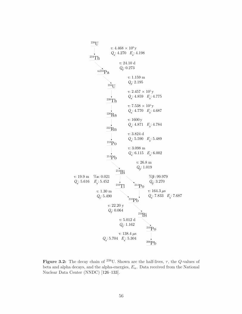
Figure 3.2: The decay chain of 238U. Shown are the half-lives, τ , the Q-values ofbeta and alpha decays, and the alpha-energies, Eα. Data received from the NationalNuclear Data Center (NNDC) [126–133].
56

types of radiation can be removed using PSD, but care is taken to reduce these
events as they degrade the WIMP sensitivity and detector livetime. The water
shield surrounding DEAP-3600 will be able to block β and γ particles and the
active veto system will be able to tag the cosmic backgrounds. Components
inside the water shield will have to be made as radiopure as possible and re-
maining events will have to be dealt with using PSD (and the acrylic shielding
in the case of βs).
An additional source of β radiation is 39Ar. This isotope is produced in
the atmosphere by interactions with high-energy cosmic rays (neutron cap-
ture). Natural argon has a specific activity of ≈ 1 Bq/kg and a half-life of 269
years [134]. This gives argon a background rate of ≈ 107 events/keV/100 kg
argon per year, and the discrimination power against electronic recoils must
be greater than that. DEAP-3600 will use argon that is depleted in 3939 to
reduce the number of these events. Since 39Ar is cosmogenically activated,
underground sources of natural gas and CO2 have been found that contain
significantly reduced 39Ar activity than atmospheric sources. Research into
finding sources, developing extraction techniques, storing, testing, and trans-
porting the depleted argon have been carried out by the DEAP/CLEAN and
WArP collaborations and production agreements have been made to supply
all three experiments with isotropically depleted argon [135, 136].
3.0.3 Atmospheric Muons
High energy cosmic rays produce muons when they interact with the atmo-
sphere, which are a type of ionising radiation able to penetrate deep into the
earth. Atmospheric muons produce two effects in DEAP. They can create
Cherenkov radiation in the light guides, which may be removed during anal-
ysis using the Zfit calculation. To reduce their effect, the light guides have
been doped with a UV absorber. Muons also carry enough energy to pro-
57

duce neutrons from detector materials through spallation. The experiments
are shielded by the rock overburden granted by locating them at SNOLAB.
SNOLAB has the lowest muon flux of any lab currently in operation due to
its depth and high density rock. Figure 3.3 shows a comparison of other un-
derground sites. To further reduce backgrounds from atmospheric muons the
water shield that completely surround DEAP-3600 will have an active veto
system. When muon pass through the shield and enter the detector they will
produce Cherenkov radiation in the water which will be collected by an array
of PMTs which will veto the event.
Equivalent Vertical Depth (km.w.e.)2 3 4 5 6
)-1 s
-2T
otal
Muo
n F
lux
(cm
-910
-810
-710
Flat-overburdan sites
Kamioka
Gran Sasso
FrejusHomestake
WIPP
Soudan
Boulby
Sudbury
Figure 3.3: Comparison of depth and muon flux for various active undergroundfacilities. Due to differences in the rock overburden, the depth is normalised towater equivalent units to account for variations in density.
3.0.4 Neutrons
These are the most troubling background since they will mimic the high-
Fpromptof a WIMP signal. The design goal of DEAP-3600 is to have zero
neutron events. The primary method of accomplishing this is through shield-
ing and the active veto. Neutrons from external sources, such as the deck steel
and rock walls, will be blocked by the water shield, while those produced by
58

atmospheric muons will be blocked and vetoed. Neutrons created by muons
in components inside the water shield will be vetoed. However, there is an-
other source of neutron production: (α,n) reactions. These are troubling since
they cannot be completely removed. DEAP-3600 will use great amounts of
acrylic shielding to prevent neutrons from (α,n) reactions in detector materials
from reaching the LAr. Studies were done at Queen’s University to measure
the attenuation length of (α,n) neutrons and predict the absolute stopping
length of acrylic, thus, DEAP-3600 will have about 22” of acrylic between the
LAr and the steel shell and electronics. The PMTs produce the most neu-
trons with their borosilicate glass and will be faced against the light guides.
Neutrons created by the stainless steel vessel and the metal components of
the cables, bases, and PMTs will be blocked using acrylic inserts between the
light guides. Monte Carlo studies are being done to study the likelihood of
neutrons reaching the LAr through air gaps.
3.1 Analysis of High-Energy α Backgrounds in
DEAP-1
While α radiation is indistinguishable from nuclear recoils using PSD alone,
event position reconstruction and energy calculation will allow us to discrim-
inate accurately. This analysis uses these tools to study high-energy α radia-
tion from the 222Rndecay chain. The goals of this study were to determine the
sources of the αs so they could be reduced and to see whether 222Rn daughters
concentrate on the detector walls. In November, 2008, we did not recover prop-
erly from a mine-wide power outage. Upon restoring power our slow controls
(process systems, temperature, and pressure monitors) malfunctioned and the
liquid level of the nitrogen cooling bath was misrepresented. The result was a
boil-off of the LAr which escaped the detector through safety valves under the
increased pressure. After stabilising and taking data to check its consistency,
59

the argon in DEAP-1 was topped up to maintain the maximum target mass,
and a burst of α activity from 222Rn was introduced into DEAP-1. We had
been studying αs prior to this event, so we were able to identify the peaks in
the energy spectrum quickly. 222Rn contamination comes from argon, as it is
present in the argon gas’s source and transportation materials. We know it
is not supported by the detector since the initial activity decayed away in a
matter of days. The data collected gave us a unique circumstance to attempt
to distinguish the energy spectra of α radiation from short-lived 222Rn daugh-
ters originating in the LAr and those from other background sources. This
analysis focuses on background data collected from August, 2008, until just
after the argon top-up in November. For this study we supplied the PMTs
with a lower voltage than normal operation to ensure that the high energy α
particles do not saturate the PMT electronics.
222Rn decays quickly through 218Po and 214Po producing three α particles.
The final α decaying isotope is 210Po (138 days) which is supported by 210Pb
with a much longer half-life (22.3 y). The initial amount of 222Rn decays
away quickly (≈3 d) and this analysis looks closely at the daughters. The
hypothesis is that the short-lived daughters will be distinct from the long-
lived 210Po, which will end up concentrated on the surface of the detector
walls. When a 210Po on the surface decays the α will either travel away from
the wall, through the argon and be detected, or it will burrow further into
the wall and the Po nucleus may move into the argon, causing nuclear recoils.
This is a serious problem, as the recoiling nucleus from a decay may interfere
with the WIMP region of interest.
Before the November 2008 argon top-up, the energy spectrum of the back-
ground could be described by a linear combination:
dNBg
dE=
dNRn222Bg
dE+
dNPo218Bg
dE+
dNPo214Bg
dE+
dNPo210Bg
dE+
dNother
dE(3.1)
60

)rRecoil energy (keV0 2000 4000 6000 8000 10000
Eve
nts
per
44 h
ours
live
time
0
10
20
30
40
50
60
Po2
14
Po2
18
Rn2
22
Po2
10
Energy Spectra Before and After the Argon Top-up
Figure 3.4: Energy spectra of high Fprompt events in the DEAP-1 detector duringlow-voltage background runs taken during the 2008 underground run. The blue lineis the normalised spectrum before the boil-off event, Equation 3.1, and the blackline is from shortly after and is dominated by 222Rn, Equation 3.2.
Each term represents the number of event counts per energy bin due to each α
source: 222Rn and its short-lived daughters, 210Po, and all other backgrounds.
This is compared to the data taken within days of the argon addition, so
we treat the long-lived 210Po (supported by 210Pb with a 22 yr half-life) as
unaffected by the top-up. After the top-up we describe the total backgrounds
in the detector from all sources as:
dNBg
dE=
dNRn222top+Bg
dE+
dNPo218top+Bg
dE+
dNPo214top+Bg
dE+
dNPo210Bg
dE+
dNother
dE(3.2)
Both spectra are shown in Figure 3.4. The blue line contains good events
(Appendix A) with Fprompt > 0.6 from all of the low-voltage background runs
in the 2008 data, before the boil-off. The run is normalised to the livetime of
the background runs taken shortly after the argon was refilled, which is the
black line. At low energy, leakage from electromagnetic events can be seen.
Within a few days the low-voltage background spectrum returned to the levels
seen before the top-up, a strong indication that the peaks are from short-lived
61

222Rn. A list of runs used in the analysis is in Appendix B.
Since the backgrounds in the detector from sources other than 222Rnwill
be equivalent in both cases, we take the difference of the two energy spectra
to remove them. The remaining events should only be those due to 222Rn and
its short-lived daughters:
dNRn
dE=
dNRn222top
dE+
dNPo218top
dE+
dNPo214top
dE(3.3)
Figure 3.5 is the energy spectrum in DEAP-1 from only the short-lived daugh-
ters of 222Rn(Equation 3.3). It shows that the peaks representing αs from the
decay of 222Rn and 218Po are now nearly equal in height and that the 210Po
peak shows less contribution.
)rRecoil energy (keV0 2000 4000 6000 8000 10000
Eve
nts
per
44 h
ours
live
time
0
10
20
30
40
50
Po2
14
Po2
18
Rn2
22
Po2
10
Pure Rn Spectrum
Figure 3.5: Energy spectrum after subtracting the top-up radon spike from thepre-boil-off background data, Equation 3.3 = 3.2 - 3.1. This spectrum is composedof only the αs from 222Rn and its short-lived daughters.
An important clue to the nature of the radon contamination is the dif-
ference between the 214Po peak and that from 222Rn and 218Po. The smaller
214Po peak was integrated and compared to the combined peaks from 222Rn
and 218Po. The ratio between them was found to be 3.9 ± 0.5; there is only one
62

214Po decay for the two decays from 222Rn and 218Po decay. This is consistent
with the hypothesis that the radon contaminants originate in the LAr and
move to the walls of the detector. The 222Rn in the LAr would be mostly non-
reactive and uncharged, able to diffuse freely through the liquid and, therefore,
we detect all of its decays. Its daughters, however, are likely to be charged
and attracted to surface materials. A factor to explain the differences in peak
height is the lifetimes of the daughters. 218Po has a half-life of only three
minutes, so it would remain close to its parent. Some may have reached the
walls in that time, and its peak is smaller than that of 222Rn. The 214Po, how-
ever, will last for a much longer time due to the intermediate 214Pb, with a
30 minute half-life, giving it time to diffuse to a surface and remain there. This
tells us that background from long-lived daughters, 210Po, will be dominated
by activity on detector walls.
)rRecoil energy (keV0 2000 4000 6000 8000 10000
Eve
nts
per
44 h
ours
live
time
0
2
4
6
8
10
Po2
14
Po2
18
Rn2
22
Po2
10
Comparison of Background Spectrum and Normalized PureRn Spectrum
Figure 3.6: The background spectrum from before the boil-off is shown in blackwhile the pure radon spectrum is in blue. This image comparatively shows thedifferences between the two spectra after normalisation.
Using the spectrum due purely to 222Rn and short-lived daughters, we can
probe the constant backgrounds present in DEAP-1 that are less well under-
63

stood: 210Po and the other high Fprompt events. This spectrum was normalised
by comparing the integrals of the outlying 214Po peaks and then subtracted
from the background data taken before the boil-off, described by Equation 3.1.
The result is:
dNdiff
dE=
dNPo210Bg
dE+
dNother
dE(3.4)
A comparison of the background spectrum and the normalised pure radon
spectrum is shown in Figure 3.6 while the result of the subtraction is shown
in Figure 3.7. The result has a wide peak suggesting alpha interactions with
variations in light yield. The over-subtraction visible in Figure 3.7 was believed
to have been due to small shifts in energy between data collection runs. Work
on improving energy calibration has been carried out and will be discussed in
Chapter 4 where this analysis is revisited to test this hypothesis. All events
at lower energies are left unchanged, and must not be related to the 222Rn α
decays. Separating the signals due to radon α decays is successful and we see
that 210Po may be treated as a distinct and constant background source.
)rRecoil energy (keV0 2000 4000 6000 8000 10000
Eve
nts
per
44 h
ours
live
time
-2
0
2
4
6
8
10
Po2
14
Po2
18
Rn2
22
Po2
10
Background Spectrum Minus Normalized Pure Rn Spectrum
Figure 3.7: The result of subtracting the pure radon spectrum (Equation 3.3) fromthe background spectrum before the boil-off (Equation 3.1). The result is describedby Equation 3.4. Over-subtraction is visible in some regions.
64

)rRecoil energy (keV0 2000 4000 6000 8000 10000
Zfit
-30
-20
-10
0
10
20
30
0
10
20
30
40
50Po2
14
Po2
18
Po2
10
Rn2
22
Zfit vs. Recoil Energy, Before Argon Boil-off
Figure 3.8: The Zfit versus recoil energy of the high-Fprompt events described byEquation 3.1 and shown in Figure 3.4. Band-like structures appear in the lightguides at low energy and near the ends of the argon volume at all energies.
To probe the nature of the remaining events (especially between 1.5 and
4 MeV) we look to position reconstruction using Zfit. Due to variations in
the reflective surface and the difference in efficiency of each PMT the detector
centre lies at 5 ∼ 6 cm, while the windows are near −6 cm and 16 cm, and
the light guides extend an additional 15 cm. The data described by Equation
3.4 was divided into regions of distinct energy and the Zfit of each region was
studied. A plot of Zfit versus energy for the background events before the
boil-off is shown in Figure 3.8. Structure formations are immediately visible,
with events near the α energies forming bands at the windows, and lower
energy backgrounds forming bands in the light guides and on the windows.
The Zfit distribution of events for the pure radon spectrum, Figure 3.9, shows
that the events due to 222Rn and its short-lived daughters occur in the bulk of
the argon, with a small dependence on the location of the windows. The Zfit
distribution in Figure 3.10 is of events in the 210Popeak, Equation 3.4. The Zfit
distributions both before and after subtracting the pure radon backgrounds are
65
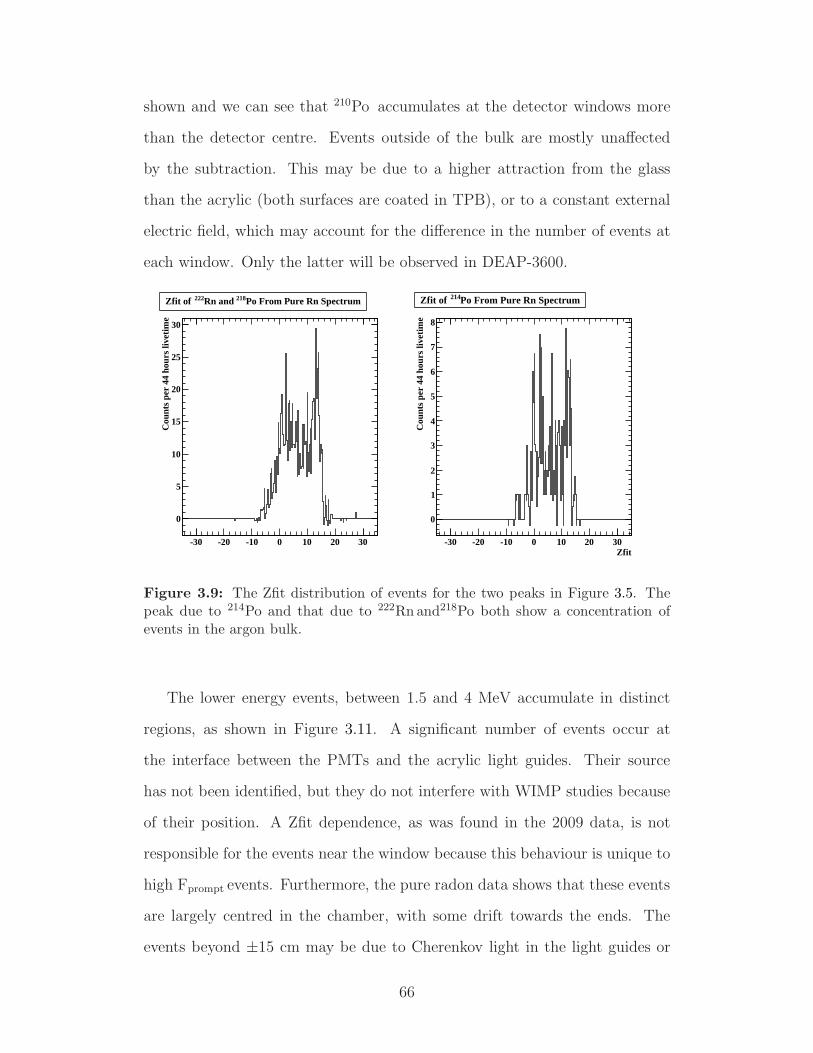
shown and we can see that 210Po accumulates at the detector windows more
than the detector centre. Events outside of the bulk are mostly unaffected
by the subtraction. This may be due to a higher attraction from the glass
than the acrylic (both surfaces are coated in TPB), or to a constant external
electric field, which may account for the difference in the number of events at
each window. Only the latter will be observed in DEAP-3600.
-30 -20 -10 0 10 20 30
Cou
nts
per
44 h
ours
live
time
0
5
10
15
20
25
30
Po From Pure Rn Spectrum218Rn and 222Zfit of
Zfit-30 -20 -10 0 10 20 30
Cou
nts
per
44 h
ours
live
time
0
1
2
3
4
5
6
7
8
Po From Pure Rn Spectrum214Zfit of
Figure 3.9: The Zfit distribution of events for the two peaks in Figure 3.5. Thepeak due to 214Po and that due to 222Rn and218Po both show a concentration ofevents in the argon bulk.
The lower energy events, between 1.5 and 4 MeV accumulate in distinct
regions, as shown in Figure 3.11. A significant number of events occur at
the interface between the PMTs and the acrylic light guides. Their source
has not been identified, but they do not interfere with WIMP studies because
of their position. A Zfit dependence, as was found in the 2009 data, is not
responsible for the events near the window because this behaviour is unique to
high Fprompt events. Furthermore, the pure radon data shows that these events
are largely centred in the chamber, with some drift towards the ends. The
events beyond ±15 cm may be due to Cherenkov light in the light guides or
66

scintillation from air, and it may be due to PMT noise. The events external
to the bulk persist in 2010 operations, while Zfit behaves differently due to
modifications made to the detector.
Zfit-30 -20 -10 0 10 20 30
Cou
nts
per
44 h
ours
live
time
0
1
2
3
4
5
6
7
8
Backgrounds, Before Boil-offαZfit of
Zfit-30 -20 -10 0 10 20 30
Cou
nts
per
44 h
ours
live
time
-1
0
1
2
3
4
5
6
7
Backgrounds, After Rn SubractionαZfit of
Figure 3.10: The Zfit distribution of events in the main α background peak. Theplot on the left shows events from the background spectrum, Equation 3.1 andFigure 3.4, and the plot on the right shows the events to long lived 210Po and otherbackgrounds, described by Equation 3.4 and shown in Figure 3.7. The pure radonspectrum has a negligible effect on events in this energy region.
3.2 Closing Remarks
This analysis successfully demonstrates that we can distinguish signals from
222Rn and its short-lived daughters from the long-living 210Po and the 210Po
may be treated as a distinct, constant background source. As a result, con-
struction of new chambers focused on limiting the amount of 210Po on the
surfaces, and an activated charcoal trap was developed to prevent 222Rn from
argon sources from entering the chamber. High energy α backgrounds were re-
duced by a factor of 10, confirming the results of this study and confirming the
hypothesis regarding the source of radon contamination. DEAP-3600 will have
the ability to clean and resurface the inner detector walls, allowing built-up α
67

Zfit-30 -20 -10 0 10 20 30
Cou
nts
per
44 h
ours
live
time
0
0.5
1
1.5
2
2.5
3
Zfit of Low-Energy Backgrounds, Before Boil-off
Zfit-30 -20 -10 0 10 20 30
Cou
nts
per
44 h
ours
live
time
0
0.5
1
1.5
2
2.5
3
Zfit of Low-Energy Backgrounds, After Rn Subraction
Figure 3.11: The Zfit distribution of lower energy events, between 1.5 and 4 MeV.The distinction between the left and right plots is the same as in Figure 3.10. Onlyevents inside the argon bulk are affected.
sources to be removed. In the following chapter this analysis will be revisited
after studying ways to make corrections to the energy calibration which was
seen to drift over time during this work. These corrections will allow for more
accurate calculations using the energy spectra presented in this chapter, and
energy calibrations based on the high energy αs will be presented.
68

Chapter 4
Relative energy corrections for
the DEAP-1 detector
The energy calibration in DEAP-1 drifts over time by a very small, but notice-
able amount. Variations in the 22Na peak position are observed in calibration
runs, which are taken with significant amount of time between them. 40K and
208Tl are detector backgrounds with Compton edges that are visible in back-
ground runs independent of the voltage supplied to the PMTs. We present a
novel function for fitting these Compton edges and results from its application.
An example of the fitter results is shown in Figure 4.1 which shows the two
Compton edges. The function does not use the TMinuit class since the χ2
distribution has many local minima that stop iterations prematurely. Instead,
we search through the χ2 distribution curve manually to determine the most
accurate value that will align the Compton edges from different runs. A run
with a known energy scale can now be used to determine an accurate keVr/pe
calibration constant for several runs. Using these calibration constants the
energy resolution is improved by between 1∼3%. The function can also reveal
information about the nature of the calibration drift and allow us to predict
and minimise it in the future and for the DEAP-3600 detector.
69

TotalPE0 100 200 300 400 500 600 700
Cou
nts
per
bin
1
10
210
310
410
Run 1360
Run 1667
Run 1667, corrected
Run 1667, corrected and vertically scaled
Example of Fitting Run 1667 to Run 1360
Figure 4.1: An example of the results of the fitter function. Run 1667 is fit to run1360, a correction factor of 1.061 is returned. The spectrum is also vertically scaledfor illustrative purposes.
4.1 Fitting Mechanism
The code was developed primarily by Minchang Zhang, a summer student
from 2009, while the work presented herein uses the tool for analysis and
background studies. The fitting function calculates a spectrum F (E; ξ) of the
number of detected photons (TotalPE) from a reference spectrum Fref(E) and
a scaling factor ξ
F (E; ξ) = n Fref
(
E
ξ
)
(4.1)
where n is an arbitrary scaling factor. The calculated histogram F (E; ξ) will
have features that match an energy spectrum that we are fitting the reference
spectrum to. The code was created for use with the ROOT data analysis
framework [137], which provides a multitude of useful classes for building data
structures and performing analysis tasks. The function is user defined and
accessed through the TFitter class by creating a TF1 object. A call to the
TH1::Fit function is never explicitly made since the TFitter and TMinuit ap-
70

proach return results dependent on the TF1 object’s initial parameters. This
is because the distribution of χ2 values for varying parameters is not smooth
and contains many local minima which TFitter finds and returns (Figure 4.2).
Since the initial parameters define where in the distribution TFitter begins to
look for the lowest χ2 value we can get inconsistent results. Many attempts
were made to overcome this, such as smoothing the 1D TotalPE histograms
that define the TF1 object, convoluting it with a Gaussian function, and mod-
ifying TFitter’s behaviour, but it was decided to bypass TFitter and perform
the χ2 search manually based on a known range that depends on the nature
of the DEAP-1 detector results. We evaluate χ2 as:
χ2 =n
∑
x=0
(
Sk(E) − Fk(E; ξ))2
Sk(E) + Fk(E; ξ)(4.2)
where Sk(E) is a static spectrum that Fref is being fit to. In this calculation
Sk(E) and Fk(E) both represent histograms corresponding to a the number
of counts at a given energy, so the dependence of the χ2 calculation on a
standard deviation of the operation is of order√
Sk(E) + Fk(E). The fitting
function returns ξ, the linear modification to TotalPE required to align the
Compton edges of the runs and uses an arbitrary vertical scaling factor n. It
is easily modified to also incorporate a horizontal translation. The vertical
scaling factor is defined by the integral of the histograms within the range of
the TF1 object.
The code is composed of four parts: the fitting function, a sorting function,
a function that calculates the χ2 result, and a main function. The sorting func-
tion determines the lowest χ2 value calculated and the fitting function defines
the TF1 object created in the main function. The main function uses user de-
fined arguments to get the runs being analysed, determine whether they were
high-voltage (HV) or low-voltage (LV) background runs, and create TChain
objects used to create the 1D TotalPE histograms that are fit to each other.
71

Figure 4.2: χ2 distribution showing large number of local minima which prema-turely stop the TFitter iterations when fitting with TMinuit in ROOT. The twopanels are the same distribution with changes to the range of Parameter0 = ξ toshow detail about the minimum.
The range of fitting depends on the voltage supplied to the PMTs and can
be changed if the function fails to fit given runs. The range of the horizontal
correction result that we are searching for is also determined manually for the
TF1 object. The initial width of this range also depends on PMT voltage
and can be adjusted if a fit fails. For example, when fitting runs of the same
type from the same operational period (2008 or 2009) we expect the Compton
edges, and the keVr/pe value, to be very close. Therefore we use a range of
0.95 to 1.05 with a 0.001 step size. When comparing runs from different op-
eration periods this range is increased to between 0.8 and 1.2 which increases
the number of steps needed for the calculations. For each step of this range
the χ2 value is calculated and stored in an array. The code may be modified
to use a smaller step size and more iterations to improve accuracy, but it was
determined that such resolution would be beyond our level of uncertainty. The
sorting function searches the χ2 distribution curve to find the lowest values. A
grid search is used with coarse intervals used first to reduce the range and then
a finer search returns the correction factor. For fitting LV to other LV runs,
the fitting interval is [200 pe, 400 pe] and the integral is taken over [220 pe,
72

480 pe]. For fitting LV runs to HV runs or fitting HV runs to other HV runs
the fitting interval is [1100 pe, 2500 pe] and the integral is taken over the same
range. We give both LV and HV histograms the same bin size and define the
range of the histograms to be from 0 pe to 700 pe (LV) or 7500 pe (HV). If
we are fitting LV runs to HV runs the LV histogram is given the same range
as the HV run.
The code is capable of fitting sets of DEAP-1 runs chained together. How-
ever, taking into account the relative corrections between the runs in a chain
has not been included. This is because recalculating the correction factors is
inefficient and a method of storing those results has not yet been decided. We
identify and use runs in sets, determined by when the data was collected. For
example, run set 2197 is a LV background run taken from April 24-27, 2009,
and consists of runs 2197 to 2202. For this set we would take each run and fit
them to 2197 (or 2198 if the first run in a set is very short). The most efficient
way to incorporate these correction factors (without modifying the code) is
to generate a set of corrected ntuple files, which store each event’s calculated
variables from the waveforms, and then analysing the larger run sets.
4.2 Limitations
When the code is implemented, the fit is not always reliable and there are
limitations on what data can be analysed. The code creates an image con-
taining the two original histograms, and the corrected histogram in order to
diagnose the goodness of fit. Often the issue is that the Compton edges have
different shapes. This can be overcome by adjusting the fitting interval man-
ually. There are several reasons why the shapes of the TotalPE spectra would
differ: if a run is very short and has low statistics, or whether there was a
problem setting up the data collection (while commissioning the VME crate,
for example). Difficulties can also show up when fitting certain LV runs to HV
73

runs or mixing the 2008 and 2009 data runs. 22Na PSD runs cannot be fit at
all using this method due to the implementation of SCA cuts which effectively
veto the high energy events in the region of the Compton edges. The 22Na cal-
ibration runs taken to analyse PSD do not have these Compton edges in their
TotalPE spectra. This is the strongest limitation, since these runs make up
the scientific regime of DEAP-1 operations. The tool will become very useful
for DEAP-3600 when the background runs are used to achieve the primary
scientific goals. Quality assurance checks should be carried out before results
of the fitting function are used in analysis.
The code has not been adapted to work with new Midas data, which re-
quires determining new ranges of integration. The next adaptation of the code
will likely be for use with the 20 inch test vessel mentioned in Section 2.5, or
with DEAP-3600.
4.3 Applications and Results
The fitting function has been primarily used in three fashions: fitting all runs
to a single run, fitting all runs to a run in their respective run sets, and
fitting the run sets to each other. Fitting the runs to a single run allows us
to investigate the way in which correction factors change over time. This can
reveal variations in detector performance and degradation of the light yield
of the liquid argon. Fitting the runs in a run set to each other and fitting
between the run sets improves the energy resolution of the detector and is
useful for background studies. Current use has been limited to low-voltage
runs and non-Midas data acquisition.
4.3.1 Correction Factors
All the low voltage background runs from 2008 and 2009 (pre-MIDAS) where
fit to run 1360. Run 1360 was taken on July 31, 2008, and has a livetime of
74

16.19 hours. It is among the earliest runs analysed. It was chosen so that we
may investigate the way the correction factors change from the start of data
taking. The variation among correction factors may be seen in Figure 4.3 with
notable events labelled.
LV runs since 13600 10 20 30 40 50 60
Tot
alP
E c
orre
ctio
ns fa
ctor
s
0.85
0.9
0.95
1
1.05
1.1
1667
VME commissioned
loss of argon and top-up, 2009
new chamber, 2009
Trend in TotalPE Correction Factors From Fitting All LV Runs to Run 1360
Figure 4.3: TotalPE correction factors from fitting every run analysed to run 1360.Steady degradation of argon light yield is seen in the 2008 run. Note that the argonloss event labelled is separate from that discussed in Chapter 3. This event was in2009, no argon spike was seen.
Figure 4.3 shows the effects that changing detector parameters have on
the TotalPE. The effects of altering the detector, such as installing the new
chamber, changing DAQ hardware, and altering the liquid level of the argon,
are quite substantial. In the 2008 data there is a steady trend of increasing
correction factors which signifies a change in the light yield from liquid argon.
Evidence of this trend has also been seen in standard detector operation and
analysis, which was a contributing factor to the decision to replace the argon
chamber and target volume. In the 2009 data we see rises and falls, which are
also seen when fitting runs in a run set to a specific run. The loss of argon
shown in graph is during 2009 and is a distinct event from that discussed in
75
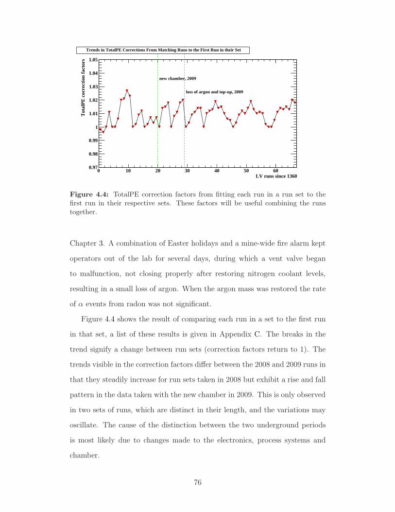
LV runs since 13600 10 20 30 40 50 60
Tot
alP
E c
orre
ctio
n fa
ctor
s
0.97
0.98
0.99
1
1.01
1.02
1.03
1.04
1.05
loss of argon and top-up, 2009
new chamber, 2009
Trends in TotalPE Corrections From Matching Runs to the First Run in their Set
Figure 4.4: TotalPE correction factors from fitting each run in a run set to thefirst run in their respective sets. These factors will be useful combining the runstogether.
Chapter 3. A combination of Easter holidays and a mine-wide fire alarm kept
operators out of the lab for several days, during which a vent valve began
to malfunction, not closing properly after restoring nitrogen coolant levels,
resulting in a small loss of argon. When the argon mass was restored the rate
of α events from radon was not significant.
Figure 4.4 shows the result of comparing each run in a set to the first run
in that set, a list of these results is given in Appendix C. The breaks in the
trend signify a change between run sets (correction factors return to 1). The
trends visible in the correction factors differ between the 2008 and 2009 runs in
that they steadily increase for run sets taken in 2008 but exhibit a rise and fall
pattern in the data taken with the new chamber in 2009. This is only observed
in two sets of runs, which are distinct in their length, and the variations may
oscillate. The cause of the distinction between the two underground periods
is most likely due to changes made to the electronics, process systems and
chamber.
76

4.3.2 Calibration of 2008 Data
Applying the correction factors plotted in Figure 4.4 to the data and then
combining runs together can improve the energy resolution of the detector
by up to 4%. We can use the radon spike discussed in Chapter 3, which
is run set 1950, to provide an accurate calibration factor for the 2008 data.
Fitting Gaussian curves to the peaks of known radionuclides, Figure 4.5, a
calibration factor for the number of photoelectrons (TotalPE) per keVr can
be calculated. The calibration factor is only valid for this run set, or runs
corrected to fit it. Run set 1950 was, therefore, additionally corrected to fit
run 1360, as are other runs, for the purpose of redoing the analysis presented
in Chapter 3. These correction factors are given in Appendix B. The radon
spike data has three distinct peaks from 222Rn, 218Po, and 214Po. The results
are plotted in Figure 4.6 and a linear fit was performed to determine the
calibration factor. The y-intercept of the fit is consistent with zero (18 ±
127 pe) so the intercept parameter was fixed at zero and the fit was repeated.
This resulted in a calibration factor with lower uncertainty that preserves the
position equivalence of the known α energies and the visible peaks in the run
set’s calibrated energy spectrum. The peak energies and keVr/pe results are
summarised in Table 4.3.2. For run sets corrected to run 1360 a keVr/pe
calibration factor of 7.20 ± 0.13 keVr/pe was found.
Radionuclide α energy (MeVr) TotalPE (pe) Width keVr/pe
222Rn 5.489 760 ± 3 33 ± 3 7.22 ± 0.31218Po 6.002 837 ± 3 21 ± 2 7.17 ± 0.18214Po 7.687 1062 ± 3 34 ± 3 7.23 ± 0.23
Table 4.1: Summary of results from fitting Gaussian functions to peaks from knownradionuclides in the TotalPE spectrum of run set 1950, after correcting each run inthe set to fit run 1950 and correcting the entire run set to fit run 1360.
77

TotalPE0 200 400 600 800 1000 1200 1400
Cou
nts
per
5.6
pe
0
10
20
30
40
50
60
Po2
14
Po2
18
Rn2
22
2008 Radon Spike Data, Corrected to Fit Run 1360
Figure 4.5: Corrected run set 1950, taken shortly after the 2008 argon top up.The peaks are fit with Gaussian functions. The effect of the corrections can be seenby comparing with Figure 3.4.
4.3.3 Analysis of α Backgrounds After Corrections
Using these correction factors the analysis presented in Chapter 3 can be
redone to see whether small changes in energy calibration account for the
over-subtraction seen before (Figure 3.7). Each run had its TotalPE corrected
and was then added to a composite spectrum for its run set. These composite
spectra were fit to run 1360 and combined to form a background spectrum
for the 2008 data. Cuts were applied to Fprompt and other data cleaning
characteristics (see Appendix A) and they were normalised by livetime. The
background spectrum was subtracted from run set 1950 to remove backgrounds
common to all 2008 detector runs and leave backgrounds introduced during
the argon top-up, resulting, once again, in a spectrum consisting of only the
fast-lived daughters of 222Rn. This pure radon spectrum was then normalised
so that its 214Po peak contained the same number of events as the same peak
in the background spectrum. Subtracting the pure radon spectrum from the
background spectrum results in the spectrum of backgrounds that are not
78

)rAlpha energy (MeV5.5 6 6.5 7 7.5
pea
ksα
Tot
alP
E fo
r
700
750
800
850
900
950
1000
1050
1100
/per 0.13 keV±Calibration factor: 7.20
Callibration of 2008 Data, Corrected to Fit Run 1360: Alpha Energy vs. TotalPE
Figure 4.6: Energy calibration of corrected 2008 TotalPE spectrum using α en-ergies. The error bars represent the widths of the Gaussian distribution fit to thepeaks.
associated with 222Rn in the argon, it is dominated by long lived 210Po on the
detector walls.
As seen in Figure 4.7, redoing the analysis after making corrections to To-
talPE does remove the over-subtraction seen in Figure 3.7. This is a significant
example of the usefulness of the fitting function results and demonstrates that
corrections to the energy resolution are needed to perform detailed analysis
of the energy spectra obtained by the detector. The remaining 210Po peak in
Figure 4.7 exhibits an asymmetry in its appearance, with more events on the
left and sharper fall on the right. This may be due to some remaining over-
subtraction from the analysis, or detector backgrounds unrelated to radon
contamination from the top up. However, detailed studies of the TPB have
been carried out within the collaboration in which the effects of α radiation
emitted from below the surface of the TPB is investigated [138, 139].
Firstly, the peak is now centred at 5.097± 0.021 keVr which is a 3.9% loss
of energy. Calculations performed with the SRIM computer program [140]
79

)rRecoil Energy (keV0 2000 4000 6000 8000 10000
Eve
nts
per
44 h
ours
live
time
-2
0
2
4
6
8
10
Po2
14
Po2
18
Rn2
22
Po2
10
Background spectrum minus normalized pure Rn spectrum after corrections
Figure 4.7: Corrected energy spectrum after subtracting the pure radon spectrum.Large over-subtractions are seen in Figure 3.4 are no longer visible.
where done to determine the energy loss of a 5.3 MeV alpha as a function of
TPB depth and found that a loss of 207 keV corresponds to a depth of about
2 µm, which implies that the 210Po may be on, or very near, the surface of
the acrylic sleeve, and that αs pass through the entire layer of TPB. Secondly,
the α leakage into the WIMP region of interest from several radionuclide-
surface geometries was investigated. Calculations of 210Po on the acrylic sleeve
ejecting αs at varying angles through the TPB show a non-Gaussian drop in
α energy below the maximum energy of the peak, consistent with the non-
linearity exhibited in all the plots presented here. Thus the asymmetry is
most likely a real effect, due to radionuclides buried beneath the TPB, and
causes α peaks to be more washed out below the peak energy due to αs taking
longer paths through the TPB. It must be emphasised that the result of this
analysis is only those 210Po events that are long-lived detector backgrounds,
activity in the LAr introduced in the spike is removed, so 210Podecays with a
full α energy are minimised. This result is also seen in the more recent detector
80

runs, although with significantly reduced α rates since new detector chamber
were constructed with the goal of reducing the amount of 210Po on the walls.
4.3.4 Calibration of 2009 Data
Calibrating the 2009 data is much more difficult because there is no event in
which a known α source was introduced during the background runs. Further-
more, we cannot rely on the 2008 calibrations since the construction process
of the new chamber has changed and the background sources are different.
We also cannot use the argon spike data since, in general, the light yield is
different and variations in the shape of the Compton edges appear between
operational periods. Methods of introducing radon to DEAP-1 towards the
end of the current underground run have been discussed, as it has proven to
be a valuable analysis tool and the long lasting effects of 210Podo not matter
since DEAP-1 will be dismantled and rebuilt with a new chamber.
Much work has been done to determine the sources of background radia-
tion in the new chamber and this calibration attempt builds off of that work.
Current models described in [141] show that the spectrum of high energy and
high Fprompt background events may be attributed to a combination of daugh-
ters of 224Ra from the decay chain of 232Th, as well as those from 222Rn seen
before. Figure 4.9 shows the results of such a model as derived from the 2009
background data, and Figure 3.1 shows the decay chain of 232Th, with energies
and half-lives. These background sources are believed to exist in the detector
materials before the chamber is constructed and deployed underground, rather
than be linked to the argon. Studies of the low-Fprompt, α-like events in the
previous run showed that there are two related sources of high energy α par-
ticles: the detector walls and the bulk argon, while utmost care was taken to
reduce the amount of contamination for the 2009 underground run.
As in section 4.3.2, each run in a set was fit to the first run in the set, and
81

TotalPE200 400 600 800 1000 1200
Cou
nts
per
5.6
pe
0
2
4
6
8
10
12
14
16
18
Events, No Relative CorrectionspromptCumulative 2009 Spectrum of High-F
Figure 4.8: The cumulative spectrum of high-Fprompt events from the 2009 under-ground run, before corrections from the fitter function are applied. Peaks from αsare not well resolved.
the runs were combined into a single TotalPE spectrum. Each of these spectra
were then fit to a common run and a cumulative background spectrum was
built. The initial effect of the energy corrections is seen in Figure 4.10. Peak
positions and widths are better resolved after applying corrections and show a
well defined peak at ≈ 860 pe. The uncorrected spectrum is shown in Figure
4.8. A set of Gaussian functions was fit to the spectrum and calibration factors
were extracted as before. These results are presented in Table 4.2. Since the
peaks may represent multiple radionuclides, weighted averages were calculated
based of the predicted number of decays from each source in [141]. The peak
positions were plotted against the suspected α energies and a linear fit was
performed. The y-intercept was consistent with zero again (−18±197) so this
parameter was again fixed at zero to prevent the results from being offset.
The 210Po peak is not well resolved in this spectrum and a Gaussian was not
well fit to it. This results in an artificially low width with a large uncertainty.
82

Figure 4.9: Model of potential background sources seen in the 2009 detector runshowing the effect of including daughters of 224Ra. From [141].
Radionuclide α energy (MeVr) TotalPE (pe) Width keVr/pe
210Po 5.304 823 ± 14 13 ± 11 6.45 ± 0.11222Rn & 224Ra 5.620 888 ± 7 45 ± 8 6.33 ± 0.05
218Po & 220Rn & 212Bi 6.206 989 ± 6 23 ± 5 6.28 ± 0.04216Po 6.778 1082 ± 9 26 ± 14 6.26 ± 0.05214Po 7.687 1217 ± 33 60 ± 72 6.31 ± 0.17
Table 4.2: Summary of results from fitting Gaussian functions to peaks fromproposed radionuclides in the cumulative TotalPE spectrum from background runstaken in 2009, after applying corrections to each run.
That the 210Po peak is overlapping the 222Rn & 224Ra peak is consistent with
the results from 2008. With this point omitted, the fit returns a calibration
factor of 6.36 ± 0.07 keVr/pe for corrected data.
There may be another peak observed below 800 pe in Figure 4.10 with a
lower energy than a 210Po α decay that is not predicted in our models. A
Gaussian was fit to this peak after calibrating the spectrum, the peak has a
mean energy of 4.92 ± 0.18 MeVr. While there are some radionuclides that
produce α radiation within 2σ of the observed peak, its integrated area is
not statistically significant compared to the background spectrum at lower
83

energies. In the decay chain of 238U, the top two parent nuclei of 222Rn both
produce radiation in this energy region. However, the half-lives of these decays
are far too long to produce significant peaks within the time scale of the
spectrum in Figure 4.10. 230Th has a half-life of 7.5 × 10⁴ y and produces a
4.687 MeV α. Its daughter is 226Ra which has a half-life of 1600 y and produces
a 4.871 MeV α when decaying into 222Rn. Another candidate is 210Bi, which
can α-decay from an excited state, but, this state is very rare and has a half-
life of 3.04 × 10⁶ y and produces a 4.946 MeV α. Its ground state, which has
a half-life of only 5.01 d, may also α-decay, but is only observed to do so on
the order of 10−4% of the time. The ejected α will have an energy of either
4.656 MeV (60%) or 4.694 MeV (40%). Other candidates are also either too
rare in nature or have too small of a chance of occurring. While the peak may
contain a couple of α events from radionuclide known to exist in the LAr, it
is more likely due to noise or is an artifact of the analysis.
TotalPE200 400 600 800 1000 1200
Cou
nts
per
5.6
pe
0
2
4
6
8
10
12
14
16
18
Po2
18, R
n220
& B
i212
Rn2
22 &
Ra2
24
Po2
14
Po2
16
Po2
10
EventspromptCumulative 2009 Corrected Spectrum of High-F
Figure 4.10: Background spectrum from 2009 after corrections, Gaussian functionsfit to notable peaks. The effect of the corrections can be seen by comparing withFigure 4.8.
84

)rAlpha energy (MeV5.5 6 6.5 7 7.5
pea
ksα
Tot
alP
E fo
r
800
900
1000
1100
1200
1300
/per 0.07 keV±Calibration factor: 6.36
Callibration of 09 Data: Alpha Energy vs. TotalPE
Figure 4.11: Energy calibration of corrected 2009 TotalPE spectrum using α
energies. The error bars represent the widths of the Gaussian distribution fit to thepeaks.
4.4 Closing Remarks
In this chapter, a novel tool for making small run-by-run corrections to the
TotalPE spectrum was presented. This tool was shown to have unexpected,
yet useful, applications; notably, its results can stand alone to qualitatively
monitor DEAP-1. The tool leads to improvements to the the energy resolution,
improving analyses based on the TotalPE variable.
We returned to the analysis presented in Chapter 3 under the prediction
that corrections to TotalPE would reduce the oversubtraction seen. It was
hoped that this effect was not due to actual events in the energy spectrum,
but an artifact left by the analysis, which was demonstrated by repeating
the analysis using the corrections. I went further and measured the peak
positions of the known α energies and determined energy calibration factors
for these data sets. These results can be combined with the results from the
fitter function and the Leff to determine accurate energy calibration factors for
individual runs in future analyses.
85

Chapter 5
Measurement of High Efficiency
Hamamatsu R877-100 PMT
A high-efficiency Hamamatsu R877-100 PMT has been delivered to the Uni-
versity of Alberta for evaluation by the DEAP collaboration. The increase in
efficiency could lead to a much greater light yield, but other experiments have
reported a slower rise time [142],[143]. We have placed the PMT in a small
dark box and had a base and preamplifier built by the Department of Physics’
Electronic Shop which will be run into either an oscilloscope or a multi-channel
analyser. With this setup we have demonstrated the PMT’s ability to distin-
guish single photoelectrons (SPE) and characterised the PMT by measuring
the SPE pulse height spectrum, the peak-to-valley ratio, the dark pulse rate,
the baseline, time resolution and SPE efficiency for varying the high voltage
supplied to the PMT.
A high efficiency PMT is desired for DEAP-3600 where light yield has
a strong effect on PSD. How well we can characterise an event depends on
the amount of light collected which makes up the pulse-shape. Many of the
design choices of DEAP-3600 have been based on how they affect light yield.
It is important to understand how these new PMTs respond to SPE, which
make up the late section of the waveforms. Understanding and correcting for
the portions of a signal due to the PMTs is crucial to PSD. Besides knowing
86
the behaviour of each PMT, detailed studies of the baselines of the DEAP-
3600 PMTs will be carried out and incorporated into the waveform analysis,
which was previously done in DEAP-1 with the Electron Tubes PMTs, and is
currently undergoing with the 8” DEAP-3600 PMTs now installed on DEAP-1.
5.1 Experimental Setup and Procedure
A single event in the DEAP-3600 detector will produce the same number of
photons as the same event in the DEAP-1 detector. In DEAP-1 these photons
are incident on only two PMTs whereas in DEAP-3600 the light will be divided
among the entire array of 266 PMTs that surround the 3600 kg target mass
of liquid argon. In order to get the most accurate results we wish to collect
as many photons as possible; how well we can characterise an event depends
on the amount of light collected which makes up the pulse-shape. DEAP-3600
will use PMTs with higher quantum efficiency than those currently used on
DEAP-1. We wish to understand the effects of a higher quantum efficiency
on the light yield of the detector and the effects that a higher light yield will
have on our ability to understand and reject background signals. A PMT with
a specifications desirable for DEAP-3600 that will fit on the smaller 5” light
guides of DEAP-1 was selected for evaluation. The increased efficiency would
lead to increased noise and the PMTs need to be understood before deploy-
ment. This work presents a series measurements performed on the selected
Hamamatsu R877-100 5” flat-faced PMT. PMTs selected for the DEAP-3600
detector will have a spherical face and large, 8” diameter. The R877-100 PMT
is similar in construction and geometry to the Electron Tubes 9390B PMTs
currently deployed on DEAP-1, using borosilicate glass and a bialkali photo-
cathode. The Hamamatsu PMT uses an advanced photocathode construction
that is calls super-bialkali (SBA) that allows the R877-100 to achieve much
higher quantum efficiency than PMTs using standard bialkali photocathodes.
87
At normal operating voltages and with ideal light sources, the Hamamatsu
R877-100 is expected to have a higher quantum efficiency of 34% compared
to 28% for the ET PMT. The Hamamatsu PMT also has a much lower gain.
The PMTs are compared at their nominal voltages, which they would oper-
ated near on DEAP-1 and are 1250 V and 1500 V for the Hamamatsu and ET
PMTs respectively.
The PMTs are powered by a variable power supply housed in a NIM crate
and we have tested the full voltage range that is specified for the PMTs. The
output of the PMT will first run through a custom built base consisting mostly
of voltage splitters for the dynodes and fewer high-voltage filters, then the sig-
nal passes through a custom built preamplifier. The preamplifier and base
were designed at the University of Alberta. Circuit diagrams for these compo-
nents are shown in Appendix E. Several spare boards (Figures. 5.1, 5.2) were
obtained for both so we remain flexible to alter the design and specifications
of either. The preamplifier is designed to produce signals desirable for DEAP-
3600; the output consists of fast pulses (≈ 100 ns) with small amplitudes for
SPE. The output of the Hamamatsu PMT is much smaller than that of the
Electron Tubes PMT, since it has a much lower gain, so a linear amplifier is
also employed when using the Hamamatsu PMT. This allows very small pulses
due to SPE (≈ −10 mV) to be recognised by the discriminators which often
have thresholds of −30 mV. The preamplifier is incorporated into the circuit
shown in Figure 5.3, which allows us to measure the response of the PMT in
several ways. From the preamplifier the signal is passed to a fan-in/fan-out
module and then either to an oscilloscope, directly to a multi-channel analyser,
or through a series of NIM logic units to count pulses or logically determine
whether the signal and was in coincidence with a light source. The MCA and
DAQ software were both developed at the University of Alberta for the radon
monitoring system to be installed in the clean-room that is under construction.
88

Depending on what we are measuring, we incorporate a discriminator, logic
units, a counter and a time to pulse height converter (TPHC). See Appendix
D for component details.
Figure 5.1: An unpopulated PMTbase.
Figure 5.2: An unpopulatedpreamplifier board.
A single setup was used for the majority of the tests, with changes to out-
puts depending on the measured quantity. The fan-in/fan-out module allowed
output from several stages to be viewed on the oscilloscope which allowed for
easy measurements and sanity checks of the data throughout the procedure.
The setup was modified when looking at time resolution to incorporate the
TPHC and an additional multi-channel analyser with different shaping char-
acteristics than our own custom designed MCA. These components were not
kept online at all times since the preamplifier discriminator was needed to set
up coincidence logic on the oscilloscope. When using the Hamamatsu PMT, a
vital component of the setup was a second channel of the fan-in/fan-out used
to control the offset of the baseline of the pulses. With careful tuning this al-
lowed the discriminator, with a threshold of −30 mV, to recognise very small
amplitude pulses (this was not necessary for the ET PMT). A comprehensive
schematic of the entire setup is shown in Figure 5.3 with the TPHC included.
The spectra were measured in 50 V steps, varying the voltage supplied to the
89

PMT from 1050 V to 1600 V for the Hamamatsu PMT and from 1300 V to
1750 V for the ET PMT. The range of HV used for the ET PMT is limited
to the range of channels that the MCA can use for its very large pulses. The
higher gain of the ET PMT can also produce large enough raw pulses to satu-
rate the preamplifier which sets a limit on the range of HV at around 1800 V,
still below the maximum rating. The effects of this can be seen in Section
5.2.1.
Figure 5.3: Schematic of electronics used to test the Hamamatsu and ElectronTubes PMTs. See Appendix D for details about the components used.
Testing was conducted in three stages, the first being in a completely dark
state, followed by the use of an LED and then a test of the timing resolution.
The first measurements were of the dark pulse rate and the spectrum of dark
pulse amplitudes. The PMT signal was passed through the preamplifier (and
linear amp for the Hamamatsu tube) and then through the fan-in/fan-out
and into the discriminator and MCA. The discriminator output pulses were
counted with the counter for each supplied high-voltage (HV) increment and
a spectrum of dark pulses was generated by the MCA and recorded on a
90

computer.
The PMT response to single photoelectrons was measured in the second set
of measurements. An LED was used to produce SPE and a precise coincidence
test was set up using a logic unit. Since the time between LED flashes and
PMT pulses varies with the HV supplied to the PMTs, the timing of pulses
and gates had to be changed for each HV. An output of the LED’s pulse
generator was passed through a fan-in/fan-out module and then to a gate
stretcher and discriminator. This allowed for narrow pulses corresponding to
the LED flashes that occur within the time interval of the PMT response. A
logic unit takes this modified LED signal and the discriminated PMT signal
and is used as a trigger for the MCA. The oscilloscope also triggers on the
coincidence between the modified PMT pulses and the PMT response. Pulse
traces for 10,000 triggered events were averaged with an oscilloscope. The
averaged traces show the PMT response to SPE. Signals due to noise and
multiple photons are statistically suppressed in the average. This allows us
to measure the baseline, and, by comparing the pulses from both PMTs, a
qualitative assessment of the effect due to electronics (base and preamplifier)
can be made. The data from both the MCA and oscilloscope will be used
to determine the average pulse amplitude due to SPE. A further test of the
relative efficiency was be done using the trigger. The LED amplitude was set
to produce about one PMT trigger for every 50 LED flashes at nominal voltage
(1250 V and 1500 V for the Hamamatsu and ET PMTs, respectively). With
the LED amplitude fixed, the PMT high voltage was varied and the change
in the ratio was recorded. This gave a measurement of how much the signal
yield for a consistent amount of light varies with HV.
The third set of measurements investigates the relationship between vary-
ing HV and the time response of the PMTs. The LED flashes are passed to
the ‘start’ input of the TPHC and the PMT discriminator pulses are passed to
91

the ‘stop’ input. The TPHC delivers pulses whose amplitude depends on the
time difference between the ‘start’ and ‘stop’ signals to a Spectrum Techniques
computer spectrometer which generates a spectrum of time differences.
5.2 Measurements and Results
5.2.1 Dark Pulse Height Spectrum
In each run pulses were collected by the MCA for four minutes at each HV.
The spectra of amplitudes for each HV are shown in Figures 5.5 and 5.6 for
the Hamamatsu and ET PMTs, respectively. The MCA is calibrated using
pulses whose amplitudes are measured independently. A calibration factor
of −0.5320 ± 0.0003 mV/channel with an offset of 103.4 ± 0.7 channels was
determined. The signals from the PMT preamplifier (and linear amplifier in
the case of the Hamamatsu PMT) split with a fan-in/fan-out module and
passed directly into the MCA for this test. A simplified schematic of this
setup can be seen in Figure 5.4.
Figure 5.4: Schematic of the NIM configuration for measuring the dark pulse ratewith a discriminator and counter and for collecting the dark spectra with an MCA.The linear amplifier is only used in conjunction with the Hamamatsu R877-100PMT. See Appendix D for details about the components used.
These spectra are composed of two distinct peaks: a low voltage noise
peak with a large number of events, and a higher voltage event peak, which
is emphasised by the range of the plots. An ideal PMT would have all PE
92
signals in the event peak and no noise. As HV increases, the position of the
event peak moves to a higher voltage. Using ROOT, a polynomial of degree
four was fit to the local maximum and minimum at amplitudes above the
noise peak, and from these the peak-to-valley ratios were determined for each
voltage increment. This is a suitable fit since we are only trying to determine
amplitude positions within the spectrum noise. Gaussian functions were not
used because these peaks follow an unknown distribution since the events that
make up the spectrum are unknown. For instance, pulses may be due to
light in the dark box (from scintillation, for instance) or purely electronic in
nature. The trends are plotted in Figures 5.7 and 5.8. Note the features at the
highest amplitudes of the ET spectra. This effect is due to the high gain of
the ET PMT and the corresponding high amplitude of the output signal. The
ET signals are large enough to saturate the preamplifier, giving a maximum
output. These are due primarily to high amplitude noise pulses.
The Hamamatsu PMT has a relatively steady peak-to-valley ratio until
operated at 1400 V at which point the rate of change of the height of the valley
decreases and the separation between noise and pulses becomes very broad.
Conversely, the ET PMT exhibits a rise and fall trend, an operating voltage
between 1450 V and 1650 V maximises the peak-to-valley ratio and offers the
strongest ability to tell event pulses from noise pulses. While the trend in peak
positions is very similar between the two PMTs, the largest difference affecting
the peak-to-valley ratios is the position of the noise peak in the Hamamatsu
PMT’s dark pulse spectrum. As HV is increased, the position of the noise
peak moves to higher voltage. Thus, the voltage position of the intersection
between the noise peak and the event peak follows the position of the event
peak, reducing the peak-to-valley ratio.
93

Voltage (mV)0 200 400 600 800 1000
Cou
nts
per
chan
nel
0
500
1000
1500
2000
2500
3000
3500
PMT Voltage (V)HV 1050HV 1150HV 1200HV 1250HV 1300HV 1350HV 1400HV 1450HV 1500HV 1550HV 1600
Hamamatsu R877-100: MCA Spectra With a Fixed Threshold (4 mins)
Figure 5.5: Pulse height spectra from the Hamamatsu R877-100 SBA PMT fordifferent operating voltages. Nominal voltage is 1250 V (blue).
Voltage (mV)0 200 400 600 800 1000 1200 1400
Cou
nts
per
chan
nel
0
500
1000
1500
2000
2500 PMT Voltage (V)HV 1300HV 1350HV 1400HV 1450HV 1500HV 1550HV 1600HV 1650HV 1700HV 1750HV 1800
Electron Tubes 9390B: MCA Spectra With a Fixed Threshold (4 mins)
Figure 5.6: Pulse height spectra from the Electron Tubes 9390B PMT for differentoperating voltages. Nominal voltage is 1500 V (brown). Note the difference in thenoise peak position compared to Figure 5.5.
94

Operating voltage (V)1000 1100 1200 1300 1400 1500 1600
Pea
k-to
-val
ley
ratio
1.1
1.15
1.2
1.25
1.3
1.35
1.4
1.45
Peak-to-valley Ratios for Each HV, Dark Spectra, Hamamatsu SBA PMT
Figure 5.7: Peak-to-valley ratios for the Hamamatsu PMT. The maximum ratedvoltage for the Hamamatsu PMT is 1500V. The ratio drops off for higher operatingvoltages.
Operating voltage (V)1300 1400 1500 1600 1700 1800
Pea
k-to
-val
ley
ratio
2.35
2.4
2.45
2.5
2.55
Peak-to-valley Ratios for Each HV, Dark Spectra, Electron Tubes 9390B PMT
Figure 5.8: Peak-to-valley ratios for the ET PMT for different operating voltages.The maximum for the ET PMT is not reached, but a distinct peak can be discerned.
95
5.2.2 Dark Pulse Rate
The rate of dark pulses that the PMTs produce is a very important consider-
ation when choosing a model, or testing those to be deployed. Random noise
pulses will not trigger DEAP electronics since they are unique to individual
PMTs, but will appear in the waveforms of actual events, most likely in the
late portion. These pulses will directly affect Fprompt calculations by increasing
the number of pe counted in the late light region. A dark rate of 10 kHz would
be unacceptable for DEAP-3600 since for each event we may see around 25
additional SPE from noise:
10 µs× 10 kHz = 0.1 noise pulses per event per PMT
A rate between one and 4 kHz is acceptable, which returns between one and
ten noise pulses per event. Dark noise rates are highly sensitive to operating
temperature and may be reduced by cooling the PMTs and lab temperature
could be monitored for the DEAP experiments. Individual PMTs will each
behave slightly differently in this regard, and each of the 266 delivered for
DEAP-3600 will be measured in temperature controlled environment. PMTs
with undesirably high dark noise rates would need to be discarded. If the high
QE PMTs cannot be demonstrated to have a low enough dark noise rate at
normal operating voltages, the model will not be considered for use on DEAP
experiments.
The dark pulse rate is measured by running the PMT discriminator output
pulses to a counter and counting over 96 second intervals (maximum allowed).
When using the Hamamatsu PMT, the PMT signal is run through a linear
amplifier as well as the preamplifier. Counts were taken while the MCA was
collecting the dark pulse height spectrum. The discriminator threshold is
held constant at its minimum setting of −30 mV. As the HV is increased
more noise pulses are allowed to cross the threshold and the dark pulse rate
96
increased rapidly. At nominal voltage the dark pulse rate was 2.7 kHz for the
Hamamatsu PMT (1250 V) and 1.27 kHz for the ET PMT (1500 V). These
rates may give rise to between three and seven noise pulses for an event in
DEAP-3600.
Rates may also be calculated from the dark MCA spectra for varying
thresholds. Using the determined positions of the peak and valley, rates were
calculated for each HV with thresholds set at the valley, the peak and at 1/4
and 1/2 of the peak position. For the Hamamatsu PMT, the 1/2 peak po-
sition closely lines up with the valley position and rate calculated at either
position appear closely related. The 1/4 peak position encroaches on the noise
peak resulting in larger rates, at very low HV the rate increase dramatically
to > 10 kHz.
The dark pulse rates counted with a constant voltage threshold are shown
in Figures 5.9 and 5.10 and the rates calculated from the spectra are shown
in Figures 5.11 and 5.12 for the Hamamatsu and ET PMTs respectively. As
expected, the Hamamatsu PMT exhibits higher dark rates than the ET PMT
due to its higher quantum efficiency. The rates calculated from the MCA
data are much lower than those from counting the PMT discriminator pulses.
This is partly due to the higher deadtime of the MCA, but also suggests that
many noise pulses trigger the discriminator at low HV, which must be taken
into account when setting up triggers for data taking. It is important to note
that the rates determined from the counter depend on the fixed threshold
of the discriminator, whereas those determined from integrating the spectra
have a floating threshold. This causes the rates from the counter to increases
for higher HV at much greater rate than those with the floating threshold.
Generally, we find a lower dark pulse rate for the ET PMT. This was expected
and the chosen Hamamatsu PMT is known to have the highest dark current
among all of Hamamatsu’s high quantum efficiency PMTs [144]. The ET
97

PMT exhibits a rise in dark pulse rate more closely following an exponential
function, that rises more steeply at higher HV than the Hamamatsu PMT.
5.2.3 Triggered SPE Pulse Height Spectrum
Using the LED pulser and logic unit, a second set of spectra were taken with
the MCA. These spectra are useful for calibrating DEAP electronics. Trig-
gered, recorded events will always be due to light so the PMT response will
be very similar, especially in DEAP-3600 where an event’s waveforms will be
produced by a small number of SPE in each PMT. The spectra collected for
this measurement show how low voltage thresholds can be set to trigger on
SPE, despite being in the noise region of the dark pulse spectra presented in
Section 5.2.1.
The electronics between the PMT and the MCA are similar to the setup in
Section 5.2.1 with two important additions, which can be seen in Figure 5.13.
The first is the inclusion of a delay cable long enough to slow the PMT signals
arrival at the MCA by 60 ns. For these measurements the MCA will dedicate
an input to a trigger signal, from the logic unit. When this input amplitude
crosses a threshold the MCA begins looking for a signal in the other inputs,
the PMT signal. The trigger signal, however, comes from passing the same
signal that the MCA is looking for (the PMT signal) through several NIM
modules, which will take several ns. Thus the delay cable is needed, since the
trigger signal would otherwise arrive at the MCA after the PMT signal. The
second addition is a second fan-in/fan-out stage before the PMT signal enters
the discriminator and is sent to the logic unit. We wish to be sensitive to
pulses over a full range of amplitudes, but with such a setup the logic unit will
only recognise pulses that cross the discriminator’s −30 mV threshold, which
is unacceptable when studying the Hamamatsu PMT. The fan-in/fan-out has
an offset adjustment that can be adjusted such that even the smallest pulses
98

Operating voltage (V)1000 1100 1200 1300 1400 1500 1600
Dar
k pu
lse
rate
(kH
z)
2
4
6
8
10
12
14
Dark Pulse Rate for Hamamatsu R877-100 SBA PMT
Figure 5.9: Hamamatsu PMT: dark rate for different operating voltages deter-mined by counting PMT discriminator pulses with a minimal, constant threshold.
Operating voltage (V)1300 1400 1500 1600 1700 1800 1900
Dar
k pu
lse
rate
(kH
z)
1
2
3
4
5
6
7
Dark Pulse Rate for Electron Tubes 9390B PMT
Figure 5.10: Electron Tubes PMT: dark rate for different operating voltages deter-mined by counting PMT discriminator pulses with a minimal, constant threshold.
99

Operating voltage (V)1000 1100 1200 1300 1400 1500 1600
Dar
k ra
te (
kHz)
1
1.5
2
2.5
3
3.5
4
4.5 Threshold positionValley1/4 SPE amplitude1/2 SPE amplitudeAverage SPE amplitude
Dark Rates Calculated from MCA Data for Different Thresholds
Figure 5.11: Hamamatsu PMT: rate of MCA dark spectrum events determinedfor varying thresholds at different operating voltages.
Operating voltage (V)1300 1400 1500 1600 1700 1800
Dar
k ra
te (
kHz)
0
0.5
1
1.5
2
2.5
3
3.5 Threshold positionValley1/4 SPE amplitude1/2 SPE amplitudeAverage SPE amplitude
Dark Rates Calculated From MCA Data for Different Thresholds
Figure 5.12: Electron Tubes PMT: rate of MCA dark spectrum events determinedfor varying thresholds at different operating voltages.
100
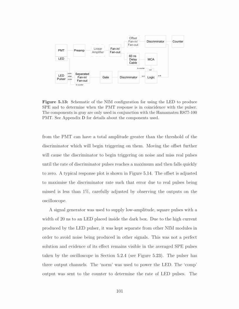
Figure 5.13: Schematic of the NIM configuration for using the LED to produceSPE and to determine when the PMT response is in coincidence with the pulser.The components in gray are only used in conjunction with the Hamamatsu R877-100PMT. See Appendix D for details about the components used.
from the PMT can have a total amplitude greater than the threshold of the
discriminator which will begin triggering on them. Moving the offset further
will cause the discriminator to begin triggering on noise and miss real pulses
until the rate of discriminator pulses reaches a maximum and then falls quickly
to zero. A typical response plot is shown in Figure 5.14. The offset is adjusted
to maximise the discriminator rate such that error due to real pulses being
missed is less than 1%, carefully adjusted by observing the outputs on the
oscilloscope.
A signal generator was used to supply low-amplitude, square pulses with a
width of 20 ns to an LED placed inside the dark box. Due to the high current
produced by the LED pulser, it was kept separate from other NIM modules in
order to avoid noise being produced in other signals. This was not a perfect
solution and evidence of its effect remains visible in the averaged SPE pulses
taken by the oscilloscope in Section 5.2.4 (see Figure 5.23). The pulser has
three output channels. The ‘norm’ was used to power the LED. The ‘comp’
output was sent to the counter to determine the rate of LED pulses. The
101

Fan-in/fan-out offset (mV)-16 -14 -12 -10 -8 -6 -4 -2 0
Rat
e of
dis
crim
inat
or p
ulse
s (k
Hz)
0
2
4
6
8
10
Typical PMT Discriminator Response to Fan-in/fan-out Offset
Figure 5.14: Typical response curve of the fan-in/fan-out offset on the rate of PMTdiscriminator pulses. The rate flattens off to the dark pulse rate corresponding tothe HV supplied to the PMT when the offset amplitude decreases.
‘initial’ output, with a delay of 0 ns, was used by the logic unit to test when
pulses generated a PMT response in coincidence.
This was done by comparing the count rate of the PMT to that of the
pulser and reducing the pulse LED amplitude until we were confident that
only SPE were being produced.
There is a measurable time difference between the LED flashes and the
PMT response, which is investigated in Section 5.2.7. The logic unit requires
both signals to overlap within a pulse width. The LED signal was delayed to
achieve this. It was passed though a gate generator, which stretched the pulse,
and into a discriminator channel. This had the effect of producing a narrow
pulse at the same time as the PMT response. The widths of the gate and
discriminators were tuned with the oscilloscope. The gate was 130 to 175 ns
wide for the Hamamatsu PMT and longer for the ET PMT. The width of
the LED discriminator was made wide, 54 ns, allowing the time of the PMT
discriminator pulse to vary, while still being recognised as in-coincidence by
102

the logic unit. The LED discriminator was set narrower, 21 ns, and fell within
the PMT discriminator signal. Widths were set as small as possible, such that
the error in counting pulses was less that 1% as determined by viewing a large
sample of random oscilloscope traces. This was done with the LED amplitude
set very high, with a coincidence rate of one PMT pulse for every two LED
flashes, so that the position of PMT pulses relative to LED flashes was clear.
Once widths were adjusted, the offset of the second fan-in/fan-out stage that
the linear amplifier runs into was adjusted when using the Hamamatsu PMT.
The counter measures the ratio between the rate of output signals from
the logic unit and the rate of the LED pulser, which was ≈ 100 kHz. The rate
counted for the PMT discriminator was fairly consistent for the entire HV
range at about ≈ 20 kHz. This is much larger than the dark rate measured for
each HV and is due to a very low discriminator threshold. The amplitude of the
LED pulser is reduced until the ratio between in-coincidence PMT responses
and LED flashes is ≈ 1/50. Such a low rate of PMT responses ensures that
when the LED is sent a signal it generates one or fewer photoelectrons. In
general LED flashes will produce very little light. While there is no guarantee
that multiple photons were not produced, the number of pulses analysed will
statistically limit the analysis to SPE.
The spectra collected show the PMT response to SPE, with either very
small noise peaks visible, or none at all. The noise reduction is not due to the
coincidence setup, low amplitude noise pulses will still occur in coincidence
with the LED at a very low rate. Since the MCA is being triggered with a
coincidence between the LED pulse and the PMT response, the MCA will not
collect pulses that are not large enough to trigger the discriminator used in the
coincidence setup. The spectra for each PMT are shown in Figures 5.15 and
5.16. The MCA threshold was set to the minimum channel possible and the
voltage at which the hardware thresholds come in can be seen in the spectra.
103

The threshold of the PMT hardware, though minimised, was greater than that
of the MCA.
Gaussian curves were fit to the peaks, and the mean in mV was calculated.
A measure of the average SPE pulse height is also obtained from the aver-
aged waveforms captured with the oscilloscope (Section 5.2.4). Averaging the
SPE pulses was done concurrently with this test, with coincidence logic being
handled by the oscilloscope’s internal triggers. The two measurements differ,
and the cause was thoroughly investigated. A very careful calibration of the
MCA was undertaken, and the oscilloscope traces were analysed in ROOT,
with baseline offsets accounted for. The measurements were determined to be
sound, and differences are due to hardware, likely being attributed to the way
the MCA may measure maxima in signal noise, the way the averaged wave-
forms have noise removed, and the way that pulse triggers on the oscilloscope
have a fixed position. Additionally, the mode of the MCA spectrum can be
measured to compliment the mean given by the Gaussian curve.
A fourth set of measurements are the peak positions of the dark MCA spec-
tra (Section 5.2.1). The average SPE pulse heights are shown in Figure 5.17.
Uncertainties are only visible for the mean of the LED triggered spectra, and
are the standard deviation (sigma) of the Gaussian function fit to the spec-
trum. This standard deviation is the best measurement of dispersion of PMT
signal amplitudes attributed to SPE and is applicable as the uncertainty to all
of the measurements of average SPE pulse amplitude done. The uncertainties
in the measurements are very small since they are statistical in nature and the
sample size is very large. Peak-to-valley ratios show a very significant improve-
ment over those found from the dark spectra, however, accurately identifying
the position of the valley at low HV is not possible since the amount of noise
is small. The peak-to-valley ratios at higher HV follow the same trend as the
dark spectra, described in Section 5.2.1 and seen in Figure 5.7.
104

Voltage (mV)0 200 400 600 800 1000
Cou
nts
per
chan
nel
0
500
1000
1500
2000
2500
3000
3500
4000
4500
PMT Voltage (V)HV 1050HV 1100HV 1150HV 1200HV 1250HV 1300HV 1350HV 1400HV 1450HV 1500HV 1550
Hamamatsu R877-100: MCA SPE Spectra with LED Coincidence
Figure 5.15: With the SPE trigger setup and an LED flasher, the pulse heightspectra from the Hamamatsu R877-100 SBA PMT for different operating voltages.
Voltage (mV)0 200 400 600 800 1000 1200
Cou
nts
per
chan
nel
0
500
1000
1500
2000
2500
3000
3500
4000
4500
5000PMT Voltage (V)
HV 1300
HV 1350HV 1400
HV 1450
HV 1500HV 1550
HV 1600
HV 1650
HV 1700HV 1750
Electron Tubes 9390B: MCA SPE Spectra with LED Coincidence
Figure 5.16: With the SPE trigger setup and an LED flasher, the pulse heightspectra from the Electron Tubes 9390B PMT for different operating voltages.
105

Operating voltage (V)1000 1100 1200 1300 1400 1500 1600
Ave
rage
SP
E a
mpl
itude
(m
V)
-500
-400
-300
-200
-100
SPE amplitude sourceLED SPE, from modeLED SPE, from meanDark SPE, from modeAverage LED SPE measured on scope
Average SPE Amplitude for Hamamatsu R877-100 SBA PMT
Figure 5.17: Average SPE amplitudes determined from analysing pulses averagedwith an oscilloscope and by integrating the MCA data, both dark and in coincidencewith the LED, Hamamatsu R877-100 SBA PMT.
Operating voltage (V)1300 1400 1500 1600 1700 1800
Ave
rage
SP
E a
mpl
itude
(m
V)
-900
-800
-700
-600
-500
-400
-300
-200
-100
0 SPE amplitude sourceLED SPE, from modeLED SPE, from meanDark SPE, from modeAverage LED SPE measured on scope
Average SPE Amplitude for Electron Tubes 9390B PMT
Figure 5.18: Average SPE amplitudes determined from analysing pulses averagedwith an oscilloscope and by integrating the MCA data, both dark and in coincidencewith the LED, ET 9390B PMT.
106
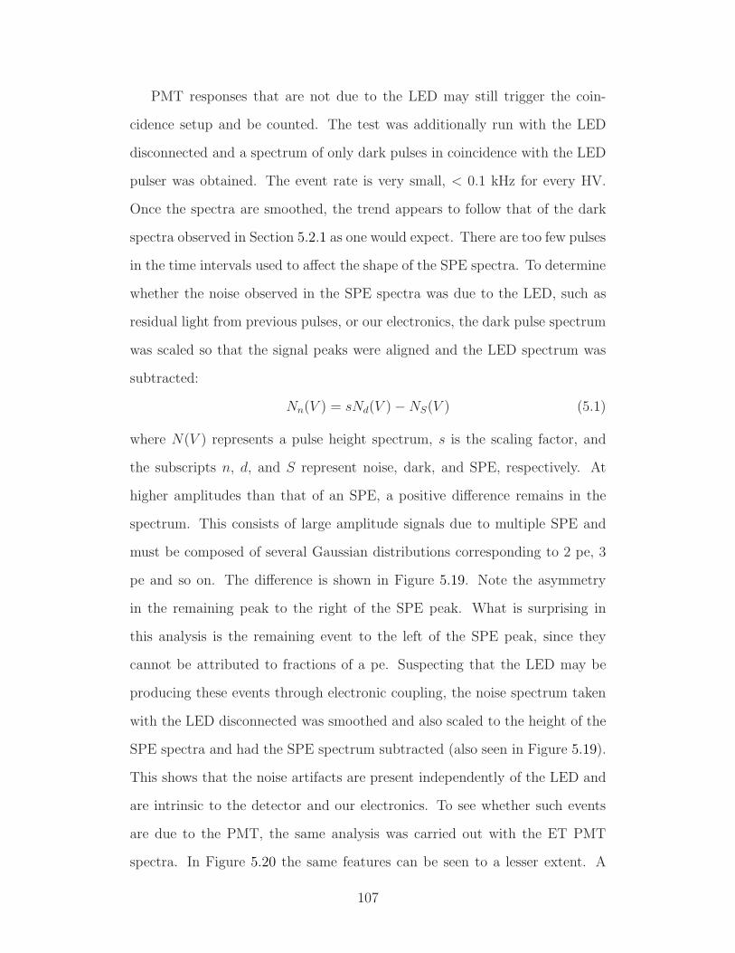
PMT responses that are not due to the LED may still trigger the coin-
cidence setup and be counted. The test was additionally run with the LED
disconnected and a spectrum of only dark pulses in coincidence with the LED
pulser was obtained. The event rate is very small, < 0.1 kHz for every HV.
Once the spectra are smoothed, the trend appears to follow that of the dark
spectra observed in Section 5.2.1 as one would expect. There are too few pulses
in the time intervals used to affect the shape of the SPE spectra. To determine
whether the noise observed in the SPE spectra was due to the LED, such as
residual light from previous pulses, or our electronics, the dark pulse spectrum
was scaled so that the signal peaks were aligned and the LED spectrum was
subtracted:
Nn(V ) = sNd(V ) − NS(V ) (5.1)
where N(V ) represents a pulse height spectrum, s is the scaling factor, and
the subscripts n, d, and S represent noise, dark, and SPE, respectively. At
higher amplitudes than that of an SPE, a positive difference remains in the
spectrum. This consists of large amplitude signals due to multiple SPE and
must be composed of several Gaussian distributions corresponding to 2 pe, 3
pe and so on. The difference is shown in Figure 5.19. Note the asymmetry
in the remaining peak to the right of the SPE peak. What is surprising in
this analysis is the remaining event to the left of the SPE peak, since they
cannot be attributed to fractions of a pe. Suspecting that the LED may be
producing these events through electronic coupling, the noise spectrum taken
with the LED disconnected was smoothed and also scaled to the height of the
SPE spectra and had the SPE spectrum subtracted (also seen in Figure 5.19).
This shows that the noise artifacts are present independently of the LED and
are intrinsic to the detector and our electronics. To see whether such events
are due to the PMT, the same analysis was carried out with the ET PMT
spectra. In Figure 5.20 the same features can be seen to a lesser extent. A
107

noticeable distinction of the ET PMT is that the widths of the dark spectra
and the LED coincidence spectra are very similar, when the difference of the
two is taken the result is very diminutive compared to that of the Hamamatsu
PMT. Since both tests were performed under conditions designed to be as
similar as possible, the much larger difference between the SPE spectrum and
the dark spectrum seen in the Hamamatsu PMT, Figure 5.19, must also be
partially due to noise. If the remaining peak was due to two or three pe, a
similar number of events would be visible in Figure 5.20 for the ET PMT,
provided the test setups were similar enough for a source to be the same for
each PMT.
The implication of this analysis is that the Hamamatsu has the ability to
produce noise at amplitudes over the range of SPE pulses. This will be prob-
lematic for DEAP-3600, since the larger noise pulses will be difficult to identify
and correct for (in terms of the baseline). The larger amplitude also has a larger
effect on Fprompt calculations. Near 50 mV, the portion of the spectra between
the low amplitude noise and the SPE amplitude exhibits a similar linear trend,
but it is very small and distinct from a spectrum of noise events below the
SPE amplitude, which peaks at about 100 mV. This suggests that some events
in this low amplitude region may be attributed to the electronics but the large
effect seen in Figure 5.19 must largely be due to the Hamamatsu PMT. Dark
noise in the PMTs comes from many sources, the most significant is thermionic
emission of electrons from the photocathode and dynodes, which is dominant
near the nominal operating voltage and increases exponentially with operating
voltage. At very low voltage ohmic leakage (current passed to the anode via
imperfect insulation) is significant, but likely not applicable in this case. At
very high voltage field emission, the emission of electrons from dynodes due
to the strong electric fields, becomes prominent. Other noise sources such as
gamma rays, scintillation in the glass envelope, ion feedback, or radiation from
108

impurities in the glass are other not considered significant in comparison, gen-
erally. The most likely increase is due increased thermionic emission from the
new material used for the SBA photocathode, combined with differences in the
Hamamatsu’s geometry. The R877-100’s dynode structure, focusing electrode
(which helps steer photoelectrons from the photocathode to the first dynode),
and the geometry of the glass envelope before the dynodes all may contribute
to an increased probability that an electron released by thermionic emission
may produce the same signal as a photoelectron. Furthermore, this result
may imply a lower uniformity of the Hamamatsu PMT, where photoelectrons
emitted from a different area of the photocathode produce position-dependent
noise amplitudes. The triggered SPE spectrum is inherently uniform, the LED
is in a fixed position and incident photons are always focused on the centre
of the photocathode. Dark noise, on the other hand may come from a source
at any point on the glass envelope, such as thermionic emissions from the
sides, rather than the photocathode, which may be amplified. Tests of unifor-
mity should be undertaken with the Hamamatsu R5912 HQE PMTs currently
installed in DEAP-1.
5.2.4 Averaged Waveforms and Baseline Determination
The baseline is the portion of a waveform before a pulse. An important quan-
tity for accurate Fprompt calculation is how well the waveform returns to the
baseline after a pulse. The average waveform after a pulse can be offset from
the baseline by a small percent of the pulse amplitude. This is often a negligi-
ble effect, but becomes significant when occurring thousands of times for each
SPE in a DEAP event. Currently, the Fprompt for DEAP-1 is calculated by
integrating the waveforms. If the baseline shifts over the range of integration,
the integrated charge due an SPE late in the tail will not be equivalent to that
in the prompt region, which directly affects Fprompt. The baseline effects due to
109

Voltage (mV)0 100 200 300 400 500 600 700 800 900
Cou
nts
per
chan
nel
0
200
400
600
800
1000
1200
1400
HV 1500 analysis
Scaled SPE spectrum
Dark spectrum
Dark spectrum with SPE spectrum subtracted
Coincident noise before and after subraction
Difference Between Dark Spectra and Scaled SPE Spectra
Figure 5.19: Analysis of noise sources by examining the difference between aspectrum taken with the LED in coincidence and a spectrum taken dark. Theresults of the same analysis taken with dark noise pulses in coincidence with theLED pulser is also shown. Performed on data collected for the Hamamatsu R877-100 SBA PMT.
the DEAP-1 PMTs have been measured and the changes are subtracted along
the waveforms before Fprompt is calculated. Another important factor is how
quickly the pulse will return to the baseline. If the pulse is too slow to return,
it can affect the next pulse, changing its amplitude and therefore impacting
the number of pe detected. Signal processing boards are being developed for
DEAP-3600 PMTs that will minimise these effects. It is important, therefore,
to understand whether the effects I see in these tests are due to the electronics
used to test the PMTs, or the PMTs themselves.
While measuring the SPE pulse height spectrum (Section 5.2.3), pulses
were also averaged and stored with an oscilloscope. The oscilloscope had
channels devoted to the same inputs as the logic unit; the discriminators for
the LED pulser and the PMT. An internal logic function was used for the
trigger, which used these inputs. The oscilloscope was used for both quality
control and to set up the logic unit that triggers the MCA. This involved
110

Voltage (mV)0 100 200 300 400 500
Cou
nts
per
chan
nel
0
200
400
600
800
1000
1200
1400HV 1500 analysis
SPE spectrum
Scaled dark spectrum
Dark spectrum with SPE spectrum subtracted
Difference Between Dark Spectra and Scaled SPE Spectra
Figure 5.20: A comparison of the analysis presented in Figure 5.19 done with theET 9390B PMT. An examination of the difference between a spectrum taken withthe LED in coincidence and a spectrum taken dark.
adjusting gate widths and pulse widths to ensure that the LED pulser and
the PMT discriminator occur within the same time interval, and ensuring
that the number of missed pulses was minimised. The coincidence circuit’s
performance was evaluated using the oscilloscope’s logic. An average of 10,000
waveforms was created and analysed in ROOT. Waveforms were recorded both
for the linear amplifier and the preamplifier for the Hamamatsu PMT (the
linear amplifier was not used with the ET PMT). The voltage per division on
the oscilloscope was kept constant and was set such that at large HV, high-
amplitude pulses would not be clipped on the oscilloscope. To see the full pulse
tail and make good measurements of the baseline, traces were made 5 µs long,
and the rate of LED pulses was 100 kHz (one pulse every 10 µs). The traces
were stored with 5000 points in 100 divisions of 50.0 ns, which corresponds
to 1.00 giga-samples per second. Pulses are ≈ 150 ns wide and their tails are
characterised by a non-smooth undershoot. A sample of pulses for different HV
(increasing HV corresponding to increasing pulse amplitude) for both PMTs
111

is shown in Figure 5.21. The common preamplifier produces very similar pulse
risetime in both PMTs. The most notable difference between the two is the
much longer tail of the ET waveforms. The preamplifier was designed to create
as close to a Gaussian-shaped pulse as possible for the Hamamatsu PMT. The
longer fall time of the ET PMT is due to greater overall charge stored in the
PMT and transferred to the electronics, a result of the high gain.
Time (ns)450 500 550 600 650 700 750 800
Vol
tage
(m
V)
-12
-10
-8
-6
-4
-2
Hamamatsu R877-100 SBA PMT
Time (ns)450 500 550 600 650 700 750 800
Vol
tage
(m
V)
-300
-250
-200
-150
-100
-50
0
Electron Tubes 9390B PMT
Figure 5.21: A sample of the average waveforms due to SPE taken with the oscil-loscope for increasing HV. The ET PMT exhibits a much longer fall time than theHamamatsu PMT and has a long tail. The risetime is dominated by the preamplifierand the fall time is dominated by the PMTs.
Attempts to fit an exponential function generally fail (large χ2/ndf) due
to features at the end of the pulse. Upon comparing the pulses from both the
Hamamatsu and ET PMTs similarities in tail shape are seen. The portions of
the waveform that are the same can be attributed to the electronics common
to both PMTs, mainly the preamplifier. Effects are much more visible in
the Hamamatsu PMT because of its lower gain. The signal from the ET
PMT is much larger than the baseline effects due to the electronics and so
the baseline effects are less visible. Because of this, the effects are easiest seen
112

at low HV on the ET PMT, whereas they become more observable at higher
HV on the Hamamatsu PMT with increasing gain. When operating the ET
PMT at very high HV fluctuations in the baseline are observed which are
caused by overloading the preamplifier as seen in Section 5.2.3. A qualitative
investigation can be done by directly comparing a waveform from each PMT.
For maximum visibility of the features, a low HV ET waveform and a high HV
Hamamatsu waveform are presented in Figures 5.22 and 5.23. The Hamamatsu
waveform has been scaled to the same amplitude as that of the ET PMT for
comparative purposes and the baselines prior to the pulse are normalised to
correspond to zero. Figure 5.22 shows the entire pulses with a narrow time
scale. An exponential function is fit to both pulses. The longer tail of the
ET PMT’s pulse follows its fit line well signifying that the pulse returns to
the baseline in a smoothly exponential fashion. The tail of the SPE pulse of
the Hamamatsu PMT, on the other hand, shows immediate signs of a non-
exponential decay. There is instead a portion of the pulse that looks linear
between 600 and 700 ns where the curve has flattened out before returning to
the baseline.
Figure 5.23 takes a closer look at the features by expanding the time range
and reducing the range of the voltage axis to regard the pulse noise. The
difference between the fit line and the SPE waveform produced by the Hama-
matsu PMT is greatly exaggerated with these axis limits. The features that
do not follow an exponential trend are clearly visible and are followed by a
slow rise back to the baseline. The shape of the features can also be seen in
the SPE waveform produced by the ET PMT at these scales, although they
are much larger and have a much longer time range. The baseline effects must
be due to the common electronics and can be reduced in future versions on
the preamplifier or signal processing boards. The increased magnitude of the
effects seen when using the ET PMT suggests that the effects are charge de-
113

pendent and are of greater concern when using PMTs with high gain. The
effects prevent analytic baseline calculations which would be used to correct
data from either DEAP-1 or DEAP-3600. An event waveform from the detec-
tors would consist of a great number of SPE pulses and each would contribute
to the overall baseline, so even a small effect would need to be corrected for.
Baseline corrections are currently numerically evaluated using detector data.
5.2.5 Gain
A measurement of the gain of both PMTs at different HV was made by inte-
grating averaged waveforms to determine the charge of an SPE. To eliminate
the effects of pulse shaping, the preamplifier was not used for this calculation
and only raw pulses were integrated. Since the raw PMT pulses of the Hama-
matsu PMT are too small to accurately measure it was analysed with the
linear amplifier, which does not change the shape of the incoming pulses. The
gain of the linear amplifier was measured using the averaged SPE waveforms
from Section 5.2.4. As the averaged waveforms were collected, the smaller
waveforms from the preamplifier were also collected and averaged in parallel.
The pulse amplitudes of both amplifiers were compared, and a linear function
was fit to the data. The fit showed that output pulses were 16.14± 0.05 times
larger than the input pulses, with an offset of 3.9 ± 0.9 mV.
Waveforms for SPE are obtained using the LED and coincidence setup at
the highest HV used during other tests; 1600 V and 1750 V for the ET PMT
and the Hamamatsu PMT respectively. To obtain raw pulses a splitter was
used at the PMT with one channel sent to the preamplifier and logic setup, to
determine which pulses are due to SPE, and the other channel sent directly to
the oscilloscope. The oscilloscope triggers on the amplified pulses like normal,
and averages of the raw pulses are made. The waveforms obtained are seen
in Figure 5.24, where the larger pulse is that on the Hamamatsu PMT which
114

Time (ns)450 500 550 600 650 700 750 800 850 900
Vol
tage
(m
V)
-80
-70
-60
-50
-40
-30
-20
-10
0
Hamamatsu R877-100 SPE pulse at 1600 V
Exponential fit line for Hamamatsu PMT
ET 9390B SPE pulse at 1300 V
Exponential fit line for ET PMT
Comparison of Waveforms and Baseline Fits for SPE Pulses
Figure 5.22: A comparison of the SPE waveforms and exponential baseline fitsof the Hamamatsu (blue) and ET (black) PMTs. Features preventing reliable fitsare clearly visible in the waveform collected for the Hamamatsu PMT. Note thedifference in pulse width and fall time.
Time (ns)500 1000 1500 2000 2500 3000
Vol
tage
(m
V)
-1
-0.8
-0.6
-0.4
-0.2
0
0.2
0.4
0.6
0.8
1
Hamamatsu R877-100 SPE pulse at 1600 V
Exponential fit line for Hamamatsu PMT
ET 9390B SPE pulse at 1300 V
Exponential fit line for ET PMT
Detail of Noise and Baseline Effects
Figure 5.23: Zoom on the y-axis of Figure 5.22, and looking at both the pulsesand tails. The same features preventing a baseline fit for the Hamamatsu PMT(near 750 ns) can be seen in different proportions on the ET PMT (between 900and 1500 ns). Issues with the Hamamatsu PMT’s baseline fit are exaggerated atthis scale. Noise caused by the high current LED pulser is visible at 350 ns.
115

passes through the linear amplifier. Note the jagged shape and large overshoot
of the raw ET PMT pulse, these characteristics are generally seen in single
ET waveforms.
Time (s)0.2 0.3 0.4 0.5 0.6 0.7 0.8 0.9 1 1.1
-610×
Vol
tage
(V
)
-0.008
-0.006
-0.004
-0.002
0
0.002
Scope Traces of Average SPE Waveforms Without the Preamplifier
Figure 5.24: Averaged raw pulses from the Hamamatsu PMT (blue) and theElectron Tubes PMT (green).
The oscilloscope traces are the time-dependent voltage V (t) = I(t)R of
the averaged pulse and are related to current I = dQ/dt. The average charge
produced in a PMT due to an SPE is calculated by integrating the averaged
waveforms.
Q =
∫
V (t)
Rdt (5.2)
The number of electrons that must be accelerated inside the PMTs by an SPE
to produce the observed charge is the gain:
GPMT =
∫
V (t) dt
eRGamp
(5.3)
where e is the electric charge and Gamp is the gain of any amplifiers used: 1
for the ET PMT and 16.14 for the Hamamatsu PMT.
For the Hamamatsu PMT the gain at 1600 V was found to be 7.52±0.08×
106 and for the ET PMT the gain at 1750 V was found to be 5.45±0.05×10⁷.
116

As expected there is an order of magnitude difference. How the gain varies
with HV will follow that of the average SPE amplitude and is shown in Figures
5.25 and 5.26. Hamamatsu reports a typical gain for the R877-100 of 3.1×10⁵
[144] at 1250 V which is about one fifth of our projected measurement of
1.5 ± 0.1 × 10⁶ at the same HV. Electron Tubes reports a typical gain of
2.7 ± 0.1 × 10⁶ for its 9390B PMT when operating at 1000 V [145]. Our
measurements do not reach such a low HV, but our projection suggests that
the gain will be < 4.6 × 10⁶, the measurement at our lowest HV of 1300 V.
Both of the reported values for gain are lower than those I measured but within
a small enough range to be acceptable. This discrepancy is acceptable since
there is very little known about the test methods used by Electron Tubes and
Hamamatsu and we are not using standard bases which affects the gain. It is
known that the PMTs are produced with varying characteristics.
5.2.6 SPE Efficiency
The SPE efficiency is a measure of how easily the PMT can identify SPE at
different operational voltages. For this set of measurements the light source
is kept constant, and the number of SPE that the PMT detects is studied.
At lower HV photons are still incident on the PMT but many go undetected,
which is undesirable for Fprompt calculation. If the SPE efficiency drops off at a
certain HV, DEAP experiments could not effectively deploy PMTs operating
below that voltage.
To measure the SPE efficiency we use the LED pulser and the coincidence
setup described in Section 5.2.3. At nominal voltage the LED amplitude is
adjusted until the ratio of PMT responses to LED flashes is ≈ 1/50. Efficiency
of the PMT varies with HV and is reflected by the changing rate of PMT
responses, R, for a fixed LED rate (RLED = 100 kHz). The HV is varied
and the change in ratio is recorded. As discussed in Section 5.2.2, data taken
117

Operating voltage (V)1000 1100 1200 1300 1400 1500 1600
)6G
ain
(x 1
0
0
1
2
3
4
5
6
7
8
Gain for Each HV for Hamamatsu R877-100 SBA PMT
Figure 5.25: Gain of the Hamamatsu R877-100 SBA PMT for different operatingvoltages.
Operating voltage (V)1300 1400 1500 1600 1700
)6G
ain
(x 1
0
0
10
20
30
40
50
60
Gain for Each HV for Electron Tubes 9390B PMT
Figure 5.26: Gain of the Electron Tubes 9390B PMT for different operating volt-ages.
118

with the counter is subject to the constant threshold of the discriminator.
A correction factor is derived from the ratio of total PMT pulses to PMT
pulses above a floating threshold. These values, Itot and Ithresh, are determined
by integrating the MCA spectra taken in coincidence with the LED (Section
5.2.3). The corrected rate from the counter becomes:
R → R′ = RIthresh
Itot
(5.4)
⇒ Eff =R
RLED
→ Eff ′ =R′
RLED
=R
RLED
Ithresh
Itot
(5.5)
The threshold used in integration is 1/2 of the position of the SPE peak. The
position of this floating threshold is arbitrarily chosen, but suitably reflects
the a proportion of pulses not counted by the counter due to the discriminator
threshold and modifies the ratio found by the counter to account for a greater
amount of low amplitude pulses being ignored by the coincidence setup at
lower HV. Results are plotted in Figures 5.27 and 5.28. Changes are generally
very small, but, are greatest between lower voltages. For the Hamamatsu
PMT, the ratio varies within a range of only 1/49 to 1/55 LED responses per
PMT flash while the ET PMT exhibited larger range 1/45 to 1/58.
5.2.7 Time Resolution
The difference in time between the LED flash and the PMT response is gen-
erally larger than the width of the amplified PMT pulse and varies with HV.
A TPHC was used to create a spectrum of pulse widths to determine how the
time difference varies with HV, and how wide the range of signal delays is for
each HV. The signals from the LED pulser and the PMT discriminator were
run into the TPHC, and the TPHC output was collected by another MCA,
a Spectrum Techniques UCS-30 universal computer spectrometer (see Figure
5.29). The change was made to accommodate the large amplitude and width of
the TPHC output pulses and to use more standard pulse shaping. The signal
119

Operating voltage (V)1000 1100 1200 1300 1400 1500 1600
Rat
io o
f PM
T p
ulse
s to
LE
D p
ulse
s
0.0155
0.016
0.0165
0.017
0.0175
SPE Efficiency of Hamamatsu R877-100 SBA
Figure 5.27: Relative efficiency of Hamamatsu R877-100 SBA PMT determinedfrom the ratio of PMT responses to LED pulses for each HV corrected for deadtime.
Operating voltage (V)1300 1400 1500 1600 1700
Rat
io o
f PM
T p
ulse
s to
LE
D p
ulse
s
0.0155
0.016
0.0165
0.017
0.0175
0.018
SPE Efficiency of Electron Tubes 9390B
Figure 5.28: Relative efficiency of Electron Tubes 9390B PMT determined fromthe ratio of PMT responses to LED pulses for each HV corrected for deadtime.
120

Figure 5.29: A simplified flowchart of the DAQ setup for measuring the timeresolution of the PMTs using a TPHC.
from the LED uses the ‘start’ input which tells the TPHC to begin looking for
a pulse from the PMT discriminator in the ‘stop’ input. The TPHC produces
a pulse whose amplitude depends on the time interval between the two mea-
surements. In order to understand the relationship between the pulse heights
and the time difference the UCS spectrometer was calibrated by using a delay
generator and the PMT discriminator. The discriminator pulse was sent to the
TPHC ‘start’ and a second discriminator output was delayed and then sent to
the TPHC’s ‘stop’ input. The time difference between the two discriminator
pulses was measured with an oscilloscope, allowing the calculation of a cali-
bration factor of 0.185± 0.001 ns/channel with an offset of −21± 1 channels.
Since the trigger places a restriction on the time interval width, none is used,
although the LED is used to produce SPE in the same manner as other tests.
The collected spectra for the two PMTs are shown in Figures 5.30 and 5.31.
The behaviour of the PMT response for both PMTs is characterised by a fast
risetime and long tail which will contain noise pulses. The background is flat
since noise pulses occur at random times after the LED flash. The spectra
imply that there is a fixed delay between an event and the response of PMT
- at a given HV a pulse within this time interval cannot be attributed to the
event. The slower falltime indicates that later pulses should be expected. The
121
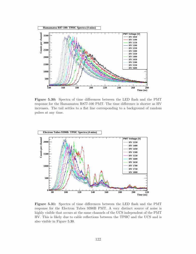
Time (ns)140 160 180 200 220 240 260 280
Cou
nts
per
chan
nel
0
500
1000
1500
2000
2500
3000
3500PMT Voltage (V)
HV 1050HV 1100HV 1150HV 1200HV 1250HV 1300HV 1350HV 1400HV 1450HV 1500HV 1550HV 1600
Hamamatsu R87-100: TPHC Spectra (4 mins)
Figure 5.30: Spectra of time differences between the LED flash and the PMTresponse for the Hamamatsu R877-100 PMT. The time difference is shorter as HVincreases. The tail settles to a flat line corresponding to a background of randompulses at any time.
Time (ns)80 100 120 140 160 180 200 220
Cou
nts
per
chan
nel
0
500
1000
1500
2000PMT Voltage (V)
HV 1350
HV 1400HV 1450
HV 1500
HV 1550HV 1600
HV 1650
HV 1700
HV 1750HV 1800
Electron Tubes 9390B: TPHC Spectra (4 mins)
Figure 5.31: Spectra of time differences between the LED flash and the PMTresponse for the Electron Tubes 9390B PMT. A very distinct source of noise ishighly visible that occurs at the same channels of the UCS independent of the PMTHV. This is likely due to cable reflections between the TPHC and the UCS and isalso visible in Figure 5.30.
122

Hamamatsu PMT has the slower response of the two, with a shortest time
interval of 162 ± 5 ns at 1600 V and a longest time interval of 197 ± 8 ns
at 1050 V. Comparatively, the ET PMT’s responses are between 96 ± 6 ns
and 119 ± 9 ns at operating voltages of 1800 V and 1300 V, respectively. A
significant source of noise shows up in the spectra collected for the ET PMT.
The noise peaks occur at the same channel for each HV and is likely due to
an undetected signal reflection either between the UCS and the TPHC. This
behaviour was undetected on the oscilloscope prior to making the measure-
ments. The noise is very large at low HV when using the ET PMT which
renders calculations made between 1300 V and 1400 V unreliable.
Time (ns)160 180 200 220 240
Vol
tage
(m
V)
0
500
1000
1500
2000
2500
3000
3500
TPHC Spectrum for Hamamatsu R877-100TPHC Spectrum for Hamamatsu R877-100
Figure 5.32: An example of the fits made to a TPHC spectrum. A line is fitbetween 10% and 90% of the peak amplitude to measure the risetime. A Gaussianfunction is fit to the rise of the peak to measure its width which corresponds therange of time differences to expect at a given HV. This spectrum was from theHamamatsu PMT operating at 1150 V.
The risetimes of the spectra were calculated by fitting a straight line to
the rise of the peak. A standard range of between 10% and 90% of the peak
amplitude was used. From the slope of the fit line the time displacement over
the range is taken to be the risetime. This risetime measurement is dominated
123

by the preamplifier, and is similar for both PMTs. An example of the fits
and analysis done with the TPHC spectra is shown in Figure 5.32. For both
PMTs the risetime becomes smaller with increasing HV. The range of risetimes
for both PMTs is only ≈ 4 ns and the value levels off above the nominal
operating voltages for both PMTs. The trend of the calculated risetimes for
the Hamamatsu PMT is shown in Figure 5.33 and that of the ET PMT is
shown in Figure 5.34. The Hamamatsu PMT has a faster risetime in general
with a range of between 12.6 ± 0.2 ns at 1050 V and 7.8 ± 0.1 ns at 1600 V.
The risetimes measured for the ET PMT range from 13.8 ± 0.5 ns at 1800 V
to 10.5 ± 0.1 ns at 1300 V.
The second measurement was made to characterise the range of time dif-
ferences between the LED and PMT events. It was known that the time
difference was non-steady as discussed in Section 5.2.3. Previous measure-
ments took this into account by allowing for coincidences to be counted within
a small interval. The spectra in Figures 5.30 and 5.31 allow for a good mea-
surement of the range of time differences to expect. A Gaussian function was
fit to the rising edge of the peak and its calculated sigma (or width) is taken to
be the expected range of time differences expected with a high certainty that
the event is not noise. The results are plotted in Figures 5.35 and 5.36 for the
Hamamatsu and ET PMTs, respectively. At higher HV the response is faster
and the widths are smaller. The widths calculated for the Hamamatsu PMT
are between 5.38±0.03 ns at 1600 V and 7.9±0.1 at 1050 V. The widths of the
ET PMT are slightly larger, between 6.41±0.04 ns at 1800 V and 8.8±0.2 ns
at 1300 V.
5.3 Closing Remarks
The Hamamatsu super-bialkali R877-100 PMT behaves well for a wide range
of operating voltages. The PMT obeys an exponential relationship between
124

Operating voltage (V)1000 1100 1200 1300 1400 1500 1600
Ris
etim
e (n
s)
8
9
10
11
12
Risetime Measurements for Hamamatsu R877-100 SBA PMT
Figure 5.33: Risetime measurement for the Hamamatsu R877-100 SBA PMTcalculated from the spectra collected using the TPHC.
Operating voltage (V)1300 1400 1500 1600 1700 1800
Ris
etim
e (n
s)
10
11
12
13
14
15
Risetime Measurement for Electron Tubes 9390B PMT
Figure 5.34: Risetime measurement for the Electron Tubes 9390B PMT calculatedfrom the spectra collected using the TPHC.
125
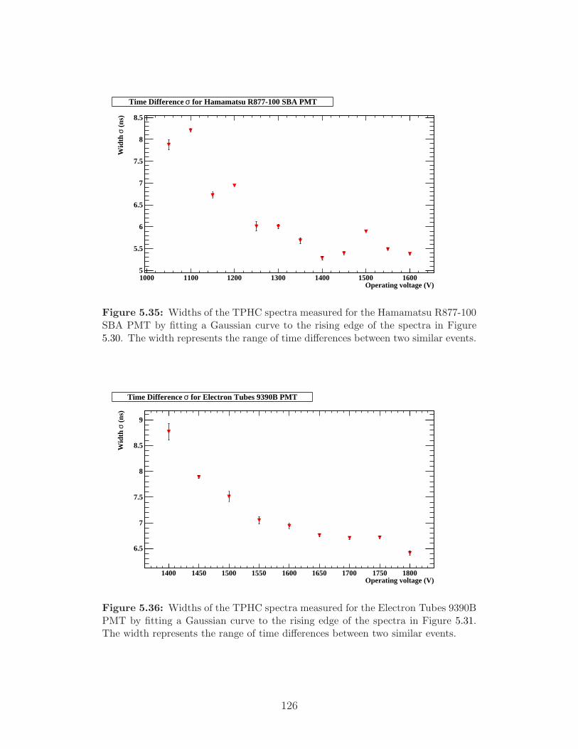
Operating voltage (V)1000 1100 1200 1300 1400 1500 1600
(ns
)σ
Wid
th
5
5.5
6
6.5
7
7.5
8
8.5
for Hamamatsu R877-100 SBA PMTσTime Difference
Figure 5.35: Widths of the TPHC spectra measured for the Hamamatsu R877-100SBA PMT by fitting a Gaussian curve to the rising edge of the spectra in Figure5.30. The width represents the range of time differences between two similar events.
Operating voltage (V)1400 1450 1500 1550 1600 1650 1700 1750 1800
(ns
)σ
Wid
th
6.5
7
7.5
8
8.5
9
for Electron Tubes 9390B PMTσTime Difference
Figure 5.36: Widths of the TPHC spectra measured for the Electron Tubes 9390BPMT by fitting a Gaussian curve to the rising edge of the spectra in Figure 5.31.The width represents the range of time differences between two similar events.
126

operating high voltage and both dark pulse rate and gain. The range of dark
pulse rates observed is between 2.04 ± 0.02 and 13.2 ± 0.3 kHz and is greater
than for the R1408 SNO PMTs, which had a range less that 5 kHz [146]. At the
nominal operating voltage and below the R877-100 PMT stays within a noise
threshold below 10 kHz. The Electron Tubes 9390B PMT is much quieter,
with a range of 1.29± 0.01 to 6.70± 0.05 kHz. The increased efficiency of the
Hamamatsu PMT should offset the larger noise by providing an increase in
light collection capability. The ET PMT has larger peak-to-valley ratios and its
noise is of lower amplitude independent of HV. It also has a faster response time
on the order of 100 ns compared to nearly 200 ns for the Hamamatsu PMT.
At higher operating voltages the PMTs respond quicker but have lower energy
resolution characterised by wide peaks in their spectra. The differences are
well understood, however, and the slower response of the Hamamatsu R877-
100 PMT should not be a problem for the applications we are considering.
This PMT follows a strongly linear relationship between the magnitude of the
source and its output voltage. The higher efficiency will improve the sensitivity
and light yield of our detectors and should not present many difficulties in its
operation and analysis.
127

Chapter 6
Conclusion
DEAP-3600 aims to either set the next lowest limit on WIMP scattering cross-
sections or make the first measurements of, and first direct detection of galactic
dark matter. It will be the lowest-background WIMP search to date, and
among the first to reach tonne-scale. The success of the experiment depends on
the PSD and most of the development work revolves around the requirements
set by it, including the work presented herein.
In Chapter 3 I analysed high-energy α backgrounds in DEAP-1. My study
helped to identify and confirm sources of backgrounds which could interfere
with WIMP signals. The result led to improvements to the detector design and
construction that will have a direct impact on DEAP-3600. These improve-
ments resulted in a reduction of high-energy, high-Fprompt backgrounds by a
factor of ten, quite significant. This analysis led also to the conclusion that
the 22Na calibration techniques we employ could be improved, since drift was
easily noticeable in the high-energy backgrounds: αs presented in Chapter 3,
and the Compton edges from βs presented in Chapter 4. A tool was developed
to align the Compton edges of background runs which leads to an improve-
ment in energy resolution of 1∼3%, which will significantly improve a WIMP
search in DEAP-3600 with continued development. The tool has shown that
it can be used to track the light-yield degradation of LAr and monitor other
128

changes to the detector.
Chapter 5 presented a detailed study of several PMT traits. These char-
acterisations will lead to a benchmark testing regime for the 8” Hamamatsu
PMTs that will be deployed on DEAP-3600. The direct comparison of the
Electron Tubes 9390B PMTs originally deployed on DEAP-1 and the high-QE
Hamamatsu R877-100 super-bialkali PMT has given the collaboration a strong
indication of what to expect when moving to high-QE PMTs for DEAP-3600.
There are two properties of the SBA PMTs that cause concern which were
investigated and measured. The first was a higher dark noise rate, found to be
approximately double that of the ET PMT. The second was a slow risetime,
which results in slower PMT responses from LED flashes. This was also shown
to be about double that of the ET PMT. The dark noise rate has been shown
to be within an acceptable range for deployment, 2.7 kHz at nominal voltage.
Pulses not observed by both DEAP-1 PMTs are vetoed, and the chance of hav-
ing noise pulses in the tail of a proper signal will be small. A larger concern
with the noise is reflected in measurements of the peak-to-valley ratios, which
imply that the Hamamatsu PMT has significantly more noise at increasing
HV, which is more likely to cross electronic thresholds and be considered an
actual pulse. The voltage response to SPE was very comparable, with sim-
ilar trends in spectrum widths. Trends in gain, relative efficiency, and SPE
amplitude were all similar as well.
DEAP-3600 will be operated with custom built signal processing boards,
which will provide pulse-shaping and amplification. It will also be run at slower
speeds, to reduce the amount of incoming data. Combined with the smaller
amount of light incident on the PMTs, these will be able to accommodate the
slower response and lower gain of the Hamamatsu SBA PMT, and the increase
in light yield resulting from the increased quantum efficiency will improve PSD,
and WIMP sensitivity.
129

Over the course of this work we have seen reductions to the backgrounds
in DEAP-1, improved our analysis methods, and seen the capability of PSD
increase by orders of magnitude. Much work is done in preparation for the
construction, commissioning, and data analysis of DEAP-3600. To that end,
my main focus has been on the PMTs. Understanding the SPE response of the
PMTs is crucial to PSD, since any pulse-tail effects will affect Fprompt calculations.
For instance, larger dark noise rates result in a greater number of noise pulses
in an event waveform, almost always in the late light region. Analysis of the
8” DEAP-3600 PMTs is ongoing on site and at collaborating institutions, and
a new result for the discrimination power is forthcoming.
130

Bibliography
[1] Kapteyn, J. C. First attempt at a theory of the arrangement and motion
of the sidereal system. Astrophys. J. 55, 302 (1922).
[2] Oort, J. The force exerted by the stellar system in the direction perpen-
dicular to the galactic plane and some related problems. Bull. Astron.
Inst. Netherlands 6, 249 (1932).
[3] Zwicky, F. Die Rotverschiebung von extragalaktischen Nebeln. Helvetica
Physica Acta 6, 110–127 (1933).
[4] Zwicky, F. Republication of: The redshift of extragalactic nebulae. Gen-
eral Relativity and Gravitation 41, 227–224 (2009). English translation
by A. Ehlers.
[5] Briel, U. G., Henry, J. P. & Boehringer, H. Observation of the Coma
cluster of galaxies with ROSAT during the all-sky survey. Astro. Astro-
phys. 259, L31–L34 (1992).
[6] White, S. D. M., Navarro, J. F., Evrard, A. E. & Frenk, C. S. The baryon
content of galaxy clusters: a challenge to cosmological orthodoxy. Nature
366, 429–433 (1993).
[7] Kubo, J. M. et al. The mass of the Coma Cluster from weak lensing
in the Sloan Digital Sky Survey. Astrophys. J. 671, 1466–1470 (2007).
0709.0506.
131

[8] Okabe, N., Okura, Y. & Futamase, T. Weak-lensing mass measurements
of substructures in Coma Cluster with Subaru/Suprime-cam. Astrophys.
J. 713, 291–303 (2010). 1001.2402.
[9] van Albada, T. S., Bahcall, J. N., Begeman, K. & Sancisi, R. Distribution
of dark matter in the spiral galaxy NGC 3198. Astrophys. J. 295, 305–
313 (1985).
[10] Babcock, H. W. The rotation of the Andromeda Nebula. Lick Obs. Bull.
19, 41–51 (1939).
[11] Rubin, V. C. & Ford, W. K., Jr. Rotation of the Andromeda Nebula
from a Spectroscopic Survey of Emission Regions. Astrophys. J. 159,
379 (1970).
[12] Rubin, V. C. & Ford, W. K., Jr. Radial Velocities and Line Strengths
of Emission Lines across the Nuclear Disk of M31. Astrophys. J. 170,
25 (1971).
[13] Freeman, K. C. On the Disks of Spiral and so Galaxies. Astrophys. J.
160, 811 (1970).
[14] Rubin, V. C., Ford, W. K., Jr. & D’Odorico, S. Emission-Line Intensi-
ties and Radial Velocities in the Interacting Galaxies NGC 4038-4039.
Astrophys. J. 160, 801 (1970).
[15] Roberts, M. S. & Rots, A. H. Comparison of Rotation Curves of Different
Galaxy Types. Astro. Astrophys. 26, 483 (1973).
[16] Einstein, A. Uber den Einfluß der Schwerkraft auf die Ausbreitung des
Lichtes. Ann. Phys. 340, 898–908 (1911).
132

[17] Dyson, F. W., Eddington, A. S. & Davidson, C. A Determination of the
Deflection of Light by the Sun’s Gravitational Field, from Observations
Made at the Total Eclipse of May 29, 1919. Phil. Trans. R. Soc. A 220,
291–333 (1920).
[18] Einstein, A. Lens-Like Action of a Star by the Deviation of Light in the
Gravitational Field. Science 84, 506–507 (1936).
[19] Zwicky, F. On the probability of detecting nebulae which act as gravi-
tational lenses. Phys. Rev. 51, 679 (1937).
[20] Walsh, D., Carswell, R. F. & Weymann, R. J. 0957 + 561 A, B - Twin
quasistellar objects or gravitational lens. Nature 279, 381–384 (1979).
[21] NASA, ACS Science Team & ESA. URL http://hubblesite.org/
gallery/album/the_universe/pr2003001e.
[22] Bacon, D. J., Refregier, A. R. & Ellis, R. S. Detection of weak grav-
itational lensing by large-scale structure. Mon. Not. R. Astron. 318,
625–640 (2000). arXiv:astro-ph/0003008.
[23] Wittman, D. M., Tyson, J. A., Kirkman, D., Dell’Antonio, I. & Bern-
stein, G. Detection of weak gravitational lensing distortions of distant
galaxies by cosmic dark matter at large scales. Nature 405, 143–148
(2000). arXiv:astro-ph/0003014.
[24] Van Waerbeke, L. et al. Detection of correlated galaxy ellipticities from
CFHT data: first evidence for gravitational lensing by large-scale struc-
tures. Astro. Astrophys. 358, 30–44 (2000). arXiv:astro-ph/0002500.
[25] Alcock, C. et al. The MACHO Project: Microlensing Results from 5.7
Years of Large Magellanic Cloud Observations. Astrophys. J. 542, 281–
307 (2000). arXiv:astro-ph/0001272.
133

[26] Tisserand, P. et al. Limits on the Macho content of the Galactic Halo
from the EROS-2 Survey of the Magellanic Clouds. Astro. Astrophys.
469, 387–404 (2007). arXiv:astro-ph/0607207.
[27] NASA & WMAP Science Team. URL http://map.gsfc.nasa.gov/
media/101080/index.html.
[28] Penzias, A. A. & Wilson, R. W. A Measurement of Excess Antenna
Temperature at 4080 Mc/s. Astrophys. J. 142, 419–421 (1965).
[29] Samtleben, D., Staggs, S. & Winstein, B. The Cosmic Microwave Back-
ground for Pedestrians: A Review for Particle and Nuclear Physicists.
Annu. Rev. Nucl. Part. Sci. 57, 245–283 (2007). 0803.0834.
[30] Komatsu, E. et al. Seven-Year Wilkinson Microwave Anisotropy Probe
(WMAP) Observations: Cosmological Interpretation. ArXiv e-prints
(2010). 1001.4538.
[31] NASA & WMAP Science Team. URL http://map.gsfc.nasa.gov/
media/080999/index.html.
[32] Lange, A. E. et al. Cosmological parameters from the first results
of Boomerang. Phys. Rev. D 63, 042001 (2001). arXiv:astro-ph/
0005004.
[33] Tucker, W. H., Tananbaum, H. & Remillard, R. A. A search for ‘failed
clusters’ of galaxies. Astrophys. J. 444, 532–547 (1995).
[34] Tucker, W. et al. 1E 0657-56: A Contender for the Hottest Known Clus-
ter of Galaxies. Astrophys. J. Lett. 496, L5 (1998). arXiv:astro-ph/
9801120.
134

[35] Clowe, D., Gonzalez, A. & Markevitch, M. Weak-Lensing Mass Recon-
struction of the Interacting Cluster 1E 0657-558: Direct Evidence for the
Existence of Dark Matter. Astrophys. J. 604, 596–603 (2004). arXiv:
astro-ph/0312273.
[36] Clowe, D. et al. A Direct Empirical Proof of the Existence of Dark
Matter. Astrophys. J. Lett. 648, L109–L113 (2006). arXiv:astro-ph/
0608407.
[37] Bradac, M. et al. Strong and Weak Lensing United. III. Measuring
the Mass Distribution of the Merging Galaxy Cluster 1ES 0657-558.
Astrophys. J. 652, 937–947 (2006). arXiv:astro-ph/0608408.
[38] NASA, Chandra X-ray Observatory Center & Space Telescope Sci-
ence Institute. URL http://hubblesite.org/newscenter/archive/
releases/2006/39/image/a/.
[39] Milgrom, M. A modification of the Newtonian dynamics as a possible
alternative to the hidden mass hypothesis. Astrophys. J. 270, 365–370
(1983).
[40] Milgrom, M. A modification of the Newtonian dynamics - Implications
for galaxies. Astrophys. J. 270, 371–384 (1983).
[41] Milgrom, M. A Modification of the Newtonian Dynamics - Implications
for Galaxy Systems. Astrophys. J. 270, 384–389 (1983).
[42] Bradac, M. et al. Revealing the Properties of Dark Matter in the Merging
Cluster MACS J0025.4-1222. Astrophys. J. 687, 959–967 (2008). 0806.
2320.
[43] Jee, M. J. et al. Discovery of a Ringlike Dark Matter Structure in the
135

Core of the Galaxy Cluster Cl 0024+17. Astrophys. J. 661, 728–749
(2007). 0705.2171.
[44] Abazajian, K. N. et al. The Seventh Data Release of the Sloan Digital
Sky Survey. Astrophys. J. Suppl. 182, 543–558 (2009). 0812.0649.
[45] Sloan Digital Sky Survey. URL http://www.sdss.org/includes/
sideimages/sdss_pie2.html.
[46] Seldner, M., Siebers, B., Groth, E. J. & Peebles, P. J. E. New reduction
of the Lick catalog of galaxies. Astro. J. 82, 249–256 (1977).
[47] de Lapparent, V., Geller, M. J. & Huchra, J. P. A slice of the universe.
Astrophys. J. Lett. 302, L1–L5 (1986).
[48] Geller, M. J. & Huchra, J. P. Mapping the universe. Science 246,
897–903 (1989).
[49] Colless, M. et al. The 2dF Galaxy Redshift Survey: spectra and red-
shifts. Mon. Not. R. Astron. 328, 1039–1063 (2001). arXiv:astro-ph/
0106498.
[50] Skrutskie, M. F. et al. The Two Micron All Sky Survey (2MASS). Astro.
J. 131, 1163–1183 (2006).
[51] Jones, D. H. et al. The 6dF Galaxy Survey: final redshift release (DR3)
and southern large-scale structures. Mon. Not. R. Astron. 399, 683–698
(2009). 0903.5451.
[52] Tegmark, M. et al. The Three-Dimensional Power Spectrum of Galaxies
from the Sloan Digital Sky Survey. Astrophys. J. 606, 702–740 (2004).
arXiv:astro-ph/0310725.
136

[53] Tegmark, M. et al. Cosmological parameters from SDSS and WMAP.
Phys. Rev. D 69, 103501 (2004). arXiv:astro-ph/0310723.
[54] Dodelson, S. & Liguori, M. Can cosmic structure form without dark
matter? Phys. Rev. Lett. 97, 231301 (2006).
[55] Jenkins, A. et al. Evolution of Structure in Cold Dark Matter Universes.
Astrophys. J. 499, 20 (1998). arXiv:astro-ph/9709010.
[56] Massey, R., NASA & ESA. URL http://hubblesite.org/
newscenter/archive/releases/2007/16/image/p/.
[57] Scoville, N. et al. The Cosmic Evolution Survey (COSMOS): Overview.
Astrophys. J. Suppl. 172, 1–8 (2007). arXiv:astro-ph/0612305.
[58] Massey, R. et al. Dark matter maps reveal cosmic scaffolding. Nature
445, 286–290 (2007). arXiv:astro-ph/0701594.
[59] Leauthaud, A. et al. Weak Gravitational Lensing with COSMOS: Galaxy
Selection and Shape Measurements. Astrophys. J. Suppl. 172, 219–238
(2007). arXiv:astro-ph/0702359.
[60] Bertone, G., Hooper, D. & Silk, J. Particle dark matter: evidence,
candidates and constraints. Phys. Rep. 405, 279–390 (2005). arXiv:
hep-ph/0404175.
[61] Jungman, G., Kamionkowski, M. & Griest, K. Supersymmetric dark
matter. Phys. Rep. 267, 195–373 (1996). arXiv:hep-ph/9506380.
[62] Weinberg, S. Approximate symmetries and pseudo-goldstone bosons.
Phys. Rev. Lett. 29, 1698–1701 (1972).
[63] Birkedal, A., Noble, A., Perelstein, M. & Spray, A. Little higgs dark
matter. Phys. Rev. D 74, 035002 (2006).
137

[64] Bergstrom, L. Non-baryonic dark matter: observational evidence and de-
tection methods. Rep. Prog. Phys. 63, 793–841 (2000). arXiv:hep-ph/
0002126.
[65] Ahlen, S. et al. The Case for a Directional Dark Matter Detector and
the Status of Current Experimental Efforts. Int J. Mod. Phys. A 25,
1–51 (2010). 0911.0323.
[66] Wikstrom, G. & Edsjo, J. Limits on the WIMP-nucleon scattering cross-
section from neutrino telescopes. J. Cosmol. Astropart. Phys. 4, 9 (2009).
0903.2986.
[67] Brunner, J. The antares neutrino telescope–status and first results. Nucl.
Instr. Meth. Phys. Res. A In Press, – (2010).
[68] EDELWEISS Collaboration. First results of the EDELWEISS-II WIMP
search using Ge cryogenic detectors with interleaved electrodes. Phys.
Lett. B 687, 294–298 (2010). 0912.0805.
[69] Cebrian, S. et al. First results of the ROSEBUD dark matter experiment.
Astropart. Phys. 15, 79–85 (2001). arXiv:astro-ph/0004292.
[70] Angloher, G. et al. Commissioning run of the CRESST-II dark matter
search. Astropart. Phys. 31, 270–276 (2009). 0809.1829.
[71] Kraus, H. et al. EURECA - The Future of Cryogenic Dark Matter
Detection in Europe. In Identification of Dark Matter 2008 (2008).
[72] Felizardo, M. et al. First Results of the Phase II SIMPLE Dark Matter
Search. ArXiv e-prints (2010). 1003.2987.
[73] Behnke, E. et al. Spin-Dependent WIMP Limits from a Bubble Cham-
ber. Science 319, 933 (2008). 0804.2886.
138

[74] Ahmed, B. et al. The NAIAD experiment for WIMP searches at Boulby
mine and recent results. Astropar. Phys. 19, 691–702 (2003). arXiv:
hep-ex/0301039.
[75] Lee, H. S. et al. Limits on Interactions between Weakly Interacting
Massive Particles and Nucleons Obtained with CsI(Tl) Crystal Detec-
tors. Phys. Rev. Lett. 99, 091301 (2007). 0704.0423.
[76] Lippincott, W. H. et al. Calibration of liquid argon and neon detectors
with 83Krm. Phys. Rev. C 81, 045803 (2010). 0911.5453.
[77] Lippincott, W. H. et al. Scintillation time dependence and pulse shape
discrimination in liquid argon. Phys. Rev. C 78, 035801 (2008).
[78] Sekiya, H. for the XMASS collaboration. XMASS. ArXiv e-prints
(2010). 1006.1473.
[79] Acciarri, R. et al. The WArP experiment. J. Phys. Conf. Ser. 203,
012006 (2010).
[80] Regenfus, C. for the ArDm Collaboration. The argon dark matter ex-
periment (ArDM). J. Phys. Conf. Ser. 203, 012024 (2010). 0912.2962.
[81] URL http://dmtools.brown.edu/. DM Tools.
[82] Savage, C., Gelmini, G., Gondolo, P. & Freese, K. Compatibility of
DAMA/LIBRA dark matter detection with other searches. J. Cosmol.
Astropart. Phys. 4, 10 (2009). 0808.3607.
[83] Ahmed, Z. for the The CDMS Collaboration. Results from the Final
Exposure of the CDMS II Experiment. ArXiv e-prints (2009). 0912.
3592.
139

[84] Aprile, E. et al. New measurement of the relative scintillation efficiency
of xenon nuclear recoils below 10 keV. Phys. Rev. C 79, 045807 (2009).
0810.0274.
[85] Aprile, E. et al. First Dark Matter Results from the XENON100 Exper-
iment. ArXiv e-prints (2010). 1005.0380.
[86] Lebedenko, V. N. et al. Results from the first science run of the ZEPLIN-
III dark matter search experiment. Phys. Rev. D 80, 052010 (2009).
0812.1150.
[87] URL http://cdms.berkeley.edu/. The CDMS collaboration home-
page.
[88] Angle, J. et al. Limits on Spin-Dependent WIMP-Nucleon Cross Sections
from the XENON10 Experiment. Phys. Rev. Lett. 101, 091301 (2008).
0805.2939.
[89] Lebedenko, V. N. et al. Limits on the Spin-Dependent WIMP-Nucleon
Cross Sections from the First Science Run of the ZEPLIN-III Experi-
ment. Phys. Rev. Lett. 103, 151302 (2009). 0901.4348.
[90] UK Dark Matter Collaboration. Limits on WIMP cross-sections from
the NAIAD experiment at the Boulby Underground Laboratory. Phys.
Lett. B 616, 17–24 (2005). arXiv:hep-ex/0504031.
[91] Archambault, S. et al. Dark matter spin-dependent limits for WIMP
interactions on 19F by PICASSO. Phys. Lett. B 682, 185–192 (2009).
0907.0307.
[92] Cooley, J. for the CDMS Collaboration. Results from the CDMS II
experiment. J. Phys. Conf. Ser. 203, 012004 (2010). 0912.1601.
140

[93] The CDMS II Collaboration. Dark Matter Search Results from the
CDMS II Experiment. Science 327, 1619 (2010).
[94] Barnabe-Heider, M. et al. Response of superheated droplet detectors of
the PICASSO dark matter search experiment. Nucl. Instr. Meth. Phys.
Res. A 555, 184–204 (2005). arXiv:physics/0508098.
[95] Aubin, F. et al. Discrimination of nuclear recoils from alpha particles
with superheated liquids. New J. Phys. 10, 103017 (2008). 0807.1536.
[96] URL http://xenon.astro.columbia.edu/. The XENON website at
Columbia.
[97] Angle, J. et al. First Results from the XENON10 Dark Matter Exper-
iment at the Gran Sasso National Laboratory. Phys. Rev. Lett. 100,
021303 (2008). 0706.0039.
[98] Bernabei, R. et al. First results from DAMA/LIBRA and the combined
results with DAMA/NaI. Eur. Phys. J. C 167 (2008). 0804.2741.
[99] Aalseth, C. E. et al. Results from a Search for Light-Mass Dark Mat-
ter with a P-type Point Contact Germanium Detector. ArXiv e-prints
(2010). 1002.4703.
[100] Collar, J. I. & McKinsey, D. N. Comments on “First Dark Matter Re-
sults from the XENON100 Experiment”. ArXiv e-prints (2010). 1005.
0838.
[101] Savage, C., Gelmini, G., Gondolo, P. & Freese, K. XENON10/100 dark
matter constraints in comparison with CoGeNT and DAMA: examining
the Leff dependence. ArXiv e-prints (2010). 1006.0972.
141

[102] Acciarri, R. et al. Oxygen contamination in liquid Argon: combined
effects on ionization electron charge and scintillation light. J. Inst. 5,
5003 (2010). 0804.1222.
[103] Acciarri, R. et al. Effects of Nitrogen contamination in liquid Argon. J.
Inst. 5, 6003 (2010). 0804.1217.
[104] Kubota, S. et al. Recombination luminescence in liquid argon and in
liquid xenon. Phys. Rev. B 17, 2716 (1978).
[105] Kubota, S., Hishida, M. & Nohara, A. Variation of scintillation decay
in liquid argon excited by electrons and alpha particles. Nucl. Instrum.
and Methods 150, 561–564 (1978).
[106] Himi, S., Takahashi, T., Ruan, J. & Kubota, S. Liquid and solid argon,
and nitrogen-doped liquid and solid argon scintillators. Nucl. Instrum.
and Methods 203, 153–157 (1982).
[107] Hitachi, A. et al. Effect of ionization density on the time dependence of
luminescence. Phys. Rev. B 27, 5279 (1983).
[108] Lide, D. R. CRC Handbook of chemistry and physics : a ready-reference
book of chemical and physical data, 90th Edition (CRC Press, 2009).
[109] Doke, T., Masuda, K. & Shibamura, E. Estimation of absolute photon
yields in liquid argon and xenon for relativistic (1 MeV) electrons. Nucl.
Instr. Meth. Phys. Res. A 291, 617–620 (1990).
[110] Nikkel, J. A., Hasty, R., Lippincott, W. H. & McKinsey, D. N. Scintilla-
tion of liquid neon from electronic and nuclear recoils. Astropart. Phys.
29, 161–166 (2008).
142

[111] Boulay, M. G. & Hime, A. Technique for direct detection of weakly
interacting massive particles using scintillation time discrimination in
liquid argon. Astropart. Phys. 25, 179 (2006).
[112] Kubota, S., Hishida, M., Suzuki, M. & Ruan, J. Dynamical behavior of
free electrons in the recombination process in liquid argon, krypton, and
xenon. Phys. Rev. B 20, 3486–3496 (1979).
[113] Boulay, M. G. et al. Measurement of the scintillation time spectra and
pulse-shape discrimination of low-energy β and nuclear recoils in liquid
argon with DEAP-1 (2009). astro-ph/0904.2930v1.
[114] Gastler, D. et al. Measurement of scintillation efficiency for nuclear
recoils in liquid argon. ArXiv e-prints (2010). 1004.0373.
[115] Doke, T. et al. Let dependence of scintillation yields in liquid argon.
Nucl. Instr. Meth. Phys. Res. A 269, 291–296 (1988).
[116] Doke, T. et al. Absolute Scintillation Yields in Liquid Argon and Xenon
for Various Particles. Jpn. J. Appl. Phys. 41, 1538 (2002).
[117] Brunetti, R. et al. WARP liquid argon detector for dark matter survey.
New Astron. Rev. 49, 265–269 (2005). arXiv:astro-ph/0405342.
[118] Pasuthip, P. Characterization os pulse-shape discrimination for back-
ground reduction in the DEAP-1 detector. Master’s thesis, Queen’s Uni-
versity (2009).
[119] Lippincott, W. H. Direct detection of dark mater with liquid argon and
neon. Ph.D. thesis, Yale University (2010).
[120] Artna-Cohen, A. Nuclear Data Sheets for A = 228. Nucl. Data Sheets
80, 723 (1997). Data extracted from the ENSDF database, revision of
Jan. 2, 1997.
143
[121] Artna-Cohen, A. Nuclear Data Sheets for A = 224. Nucl. Data Sheets
80, 227 (1997). Data extracted from the ENSDF database, revision of
Nov. 18, 1996.
[122] Artna-Cohen, A. Nuclear Data Sheets for A = 216, 220. Nucl. Data
Sheets 80, 157 (1997). Data extracted from the ENSDF database, revi-
sion of Oct. 25, 1997.
[123] Wu, S. C. Nuclear Data Sheets for A = 216. Nucl. Data Sheets 108,
1057–1092 (2007). Data extracted from the ENSDF database, revision
of March. 3, 2007.
[124] Browne, E. Nuclear Data Sheets for A = 212. Nucl. Data Sheets 104,
427–496 (2005). Data extracted from the ENSDF database, revision of
Nov. 29, 2004.
[125] Martin, M. J. Nuclear Data Sheets for A = 208. Nucl. Data Sheets 108,
1583–1806 (2007). Data extracted from the ENSDF database, revision
of June. 27, 2007.
[126] Browne, E. & Tuli, J. K. Nuclear Data Sheets for A = 234. Nucl. Data
Sheets 108, 681–772 (2007). Data extracted from the ENSDF database,
revision of Nov. 9, 2006.
[127] Akovali, Y. A. Nuclear Data Sheets for A = 230. Nucl. Data Sheets
69, 155 (1993). Data extracted from the ENSDF database, revision of
March 4, 1993.
[128] Akovali, Y. A. Nuclear Data Sheets for A = 226. Nucl. Data Sheets
77, 433 (1995). Data extracted from the ENSDF database, revision of
March 6, 1996.
144

[129] Akovali, Y. A. Nuclear Data Sheets for A = 222. Nucl. Data Sheets 77,
271 (1996). Data extracted from the ENSDF database, revision of Jan.
16, 1996.
[130] Jain, A. K. & Singh, B. Nuclear Data Sheets for A = 218. Nucl.
Data Sheets 107, 1027–1074 (2006). Data extracted from the ENSDF
database, revision of Dec. 15, 2005.
[131] Wu, S. C. Nuclear Data Sheets for A = 214. Nucl. Data Sheets 110,
681–748 (2009). Data extracted from the ENSDF database, revision of
Nov. 1, 2007.
[132] Browne, E. Nuclear Data Sheets for A = 210. Nucl. Data Sheets 99,
483–753 (2003). Data extracted from the ENSDF database, revision of
March 26, 2003.
[133] Kondev, F. G. Nuclear Data Sheets for A = 206. Nucl. Data Sheets 109,
1557–1654 (2008). Data extracted from the ENSDF database, revision
of March 24, 2008.
[134] Benetti, P. et al. Measurement of the specific activity of 39Ar in natural
argon. Nucl. Instr. Meth. Phys. Res. A 574, 83–88 (2007). arXiv:
astro-ph/0603131.
[135] Acosta-Kane, D. et al. Discovery of underground argon with low level
of radioactive 39Ar and possible applications to WIMP dark matter de-
tectors. Nucl. Instr. Meth. Phys. Res. A 587, 46–51 (2008).
[136] Mei, D. et al. Prediction of underground argon content for dark matter
experiments. Phys. Rev. C 81, 055802 (2010). 0912.5368.
[137] Brun, R. & Rademakers, F. ROOT - An object oriented data analysis
framework. Nucl. Instr. Meth. Phys. Res. A 389, 81–86 (1997).
145

[138] Cai, B., Pollman, T. & Boulay, M. Surface backgrounds in the DEAP-
3600 detector. DEAP internal document.
[139] Pollamn, T., Boulay, M. & Kuzniak, M. Scintillation of thin tetraphenyl
butadiene films under alpha particle excitation. Submitted for publication
(2010).
[140] URL http://www.srim.org/. Stopping and Range of Ions in Matter
(SRIM).
[141] Boulay, M. DEAP high and low-energy backgrounds. (2009).
URL https://www.snolab.ca/deap/private/TWiki/bin/view/Main/
BackgroundNotesAug72009. Entry on DEAP TWiki.
[142] FAT Results for high-QE DOMs. Tech. Rep. (2009). From the IceCube
wiki.
[143] Kauer, M. Calorimeter R&D for the SuperNEMO double beta decay
experiment. In XIII Int. Conf. on Calorimetry in High Energy Physics,
vol. 160, 012031 (IOP Publishing Ltd, London, 2009).
[144] Hamamatsu. UBA SBA Photomultiplier tube series (2008).
[145] Electron Tubes. 130mm (5in) photomultiplier 9390B series data sheet
(2009).
[146] The SNO detector: the photomultiplier tubes. URL http://sno.phy.
queensu.ca/sno/sno2.html. From the SNO homepage at Queen’s Uni-
versity.
146

Appendix A
Data Cleaning Cuts and Zfit
Corrections
All corrections and cuts were performed while events were being selected from
the ntuples and before being placed into histogram bins. This includes the
corrections to TotalPE. All spectra showing α peaks have a cut placed on
Fprompt, only events with Fprompt > 0.6 are considered.
Standard data cleaning cuts were performed while events were selected
from ntuples:
• abs(Edge0-1000) < 200 & abs(Edge0-Edge1) < 20
• HLatePE0 < 0 & HLatePE1 < 0
• HPromptPE0 < 0 & HPromptPE1 < 0
• EventCutID = 1
• PmtCutID0 = 7 & PmtCutID1 = 7
• abs(PreSignal0) < 0.5 & abs(PreSignal1) < 0.5
In addition to these cuts, a Zfit correction was applied to the data from
2009:
• Zfit = Zfit/(0.962-0.0013×Zfit+0.0005×Zfit2)
147

Appendix B
Run List
In Chapters 3 and 4, the following run sets were analysed. The livetime and
result from fitting the entire run sets, which use the run-by-run corrections in
Appendix C, to run 1360 are both given.
2008
Run (to) Date Livetime Fit to run 1360
1360 1361 July 31-Aug 1 56.85 1.0001667 Sept 24 48.825 1.0611818 1823 Oct 20-21 19.774 1.0061871 1874 Oct 28-29 38.497 1.0271950 1954 Nov 24-25 44.053 1.064
2009
2102 2105 March 24 37.300 1.0002151 2155 April 7 41.661 1.0112197 2202 April 24-27 57.277 1.0892300 2312 May 21-27 88.86 1.000
Table B.1: list of low-voltage runs from 2008 and 2009 used in the analyses pre-sented in Chapters 3 and 4. Included are correction factors from fitting the run setsto run 1360.
148

Appendix C
Fitter Results
The following tables are a list of individual runs analysed in Chapter 4 and
the results determined by the fitter function to line up their Compton edges
with the first run in each set.
2008
Run Correction factor
1356 0.9981357 0.9961360 1.0001361 1.0111667 1.0001818 1.0001819 1.0061820 1.0201821 1.0211822 1.0271823 1.0231871 1.0001872 1.0021873 1.0091874 1.0121950 1.0001951 1.0021952 1.0071953 1.0031954 1.007
149

2009
Run Correction factor Run Correction factor
2102 1.000 2279 1.0062103 1.014 2280 1.0052104 1.015 2300 1.0002105 1.018 2301 1.0032151 1.000 2302 1.0092152 1.008 2303 1.0122153 1.011 2304 1.0102154 1.018 2305 1.0142155 1.020 2306 1.0192197 1.000 2307 1.0132198 1.003 2308 1.0102199 1.009 2309 1.0112200 1.011 2310 1.0102201 1.014 2311 1.0022202 1.014 2312 1.0002271 1.000 2317 1.0002272 1.010 2318 1.0052273 1.012 2319 1.0112274 1.013 2320 1.0142275 1.019 2321 1.0132276 1.014 2322 1.0152277 1.015 2323 1.0132278 1.010 2324 1.020
2325 1.018
Table C.1: List of runs from the 2008 and 2009 underground runs and theircorrection factors from fitting each run to the first run in their respective run sets.The analysis is discussed in Chapter 4.
150

Appendix D
List of NIMs Used in Tests
This is list of the Nuclear Instrumentation Modules used during the tests of
both PMTs.
• HV power supply: Bertan Associates, inc. Model 375P
• Discriminator: LeCroy 623 Octal Discriminator
• Gate generator: LeCroy 222 Dual Gate Generator
• Fan-in/fan-out: LeCroy 428F Linear fan-in/fan-out (×2)
• Logic: LeCroy 365AL 4-Fold Logic Unit
• Time to pulse height converter: Ortec 437A TPHC
• Counter: Philips PM6654 Programmable high resolution timer/counter
• Pulse generator: Berkley Nucleonics Corp. 7085 Digital Delay/Width
Generator
151

Appendix E
Cicuit Diagrams for Custom
Electronics
The following are circuit diagrams for some of the electronics used for PMT
measurements that were designed and built by the Electronics Shop of the
Department of Physics at the University of Alberta. Included are the bases
for both PMTs and the preamplifer used for them. The base for the ET PMT
was designed at Queen’s University and built at the University of Alberta.
152

Figure E.1: Circuit diagram for the base used to operate the ET 9390B PMT,designed at Queen’s University.
153

5
5
4
4
3
3
2
2
1
1
D D
C C
B B
A A
Title
Size Document Number Rev
Date: Sheet of
University of Alberta Physics Electronics Shop v1.0
R877-100 PMT Base
A
2 2Thursday, August 13, 2009
Title
Size Document Number Rev
Date: Sheet of
University of Alberta Physics Electronics Shop v1.0
R877-100 PMT Base
A
2 2Thursday, August 13, 2009
Title
Size Document Number Rev
Date: Sheet of
University of Alberta Physics Electronics Shop v1.0
R877-100 PMT Base
A
2 2Thursday, August 13, 2009
All parts 350Vpeak/200V working minimum unless noted
2000V Max
R8
330k
R8
330k
C322nFC322nF
J9
CON1
J9
CON1
1
1.8Meg1.8Meg
R7
330k
R7
330k
C2
22nF
C2
22nF
C1
10nF
C1
10nF
R6
330k
R6
330k
J8
HV
J8
HV
1
R5
330k
R5
330k
C344.7nF2500V
C344.7nF2500V
R4
330k
R4
330k
C24
NS
C24
NS
R3
330k
R3
330k
C32NS
C32NS
R2
330k
R2
330k
R151MR151M
R1
330k
R1
330k
R52
10k
R52
10k
C23
10nF
C23
10nF
J1
BNC
J1
BNC
1
2
37.6nF37.6nF
C31NSC31NS
R131MR131M
R12
330k
R12
330k
C6
4.7nF2500V
C6
4.7nF2500V
R11
330k
R11
330k
R10
330k
R10
330k
R9
330k
R9
330k
DY10
DY9
DY8
DY7
DY6
DY5
DY4
DY3
DY2
DY1
P
K
G
PMT1
R877-100
DY10
DY9
DY8
DY7
DY6
DY5
DY4
DY3
DY2
DY1
P
K
G
PMT1
R877-100
11
1
2
3
4
5
6
7
8
9
10
13
14
Figure E.2: Circuit diagram for the base used to operate the Hamamatsu R877-100SBA PMT.
154

5
5
4
4
3
3
2
2
1
1
D D
C C
B B
A A
-IN
U7out
U7_NULL
U7_NULLS1_OUT
-IN
S1_OUT
+IN
U7-
S1_OUT
U11_NULL
U7+
+IN
TEST
U3+
U3-U3out
U3_NULL
U3_NULL
OFFSET
U11_NULL
+IN
-IN
U3_NULL
U3out
U3_NULL
U3+
U3-
U7out
U7_NULL
U7+
U7-
U7_NULL
5V
5V_U5
-12V
-12V_U7
-12V_U7
12V
-12V_U7
-5V_U5
5V_U5
-5V_U5
5V_U5
5V
-5V
-5V
5V
-12V
12V_U3
-5V
-5V_U5
12V_U7
12V_U7
5V 12V
-12V_U3
12V_U3
-12V_U3
+VIN
-VIN
-VIN -VIN
+VIN
+VIN
-VIN
12V
-12V
12V
+VIN
+VIN
-VIN
-12V
12V
+VIN 12V 5V
-VIN -12V -5V
-5V_U5
5V_U5
-5V_U5
5V_U5
-5V_U5
12V_U3
-12V_U3
12V_U7
-12V_U7
-12V_U3
Title
Size Document Number Rev
Date: Sheet of
1.0.0
Radon Preamp
B
1 1Tuesday, April 14, 2009
Title
Size Document Number Rev
Date: Sheet of
1.0.0
Radon Preamp
B
1 1Tuesday, April 14, 2009
Title
Size Document Number Rev
Date: Sheet of
1.0.0
Radon Preamp
B
1 1Tuesday, April 14, 2009
Title
Size Document Number Rev
Date: Sheet of
<Doc>B
1 1Tuesday, April 14, 2009
Title
Size Document Number Rev
Date: Sheet of
<Doc>B
1 1Tuesday, April 14, 2009
Title
Size Document Number Rev
Date: Sheet of
<Doc>B
1 1Tuesday, April 14, 2009
Alternate parts
Alternate parts
C16
10uF
C16
10uF
J17
GND
J17
GND
1
R3032.4kR3032.4k
R64.84kR64.84k
L1
10uH
L1
10uH
R2710k
R2710k
L2
200MA-750
L2
200MA-750
J5
CON2
J5
CON2
12
+
-
U4
AD817/AD711
+
-
U4
AD817/AD711
3
26
74
18 5
C14
NS
C14
NS
C11
1pF
C11
1pF
J4
Monitor
J4
Monitor
R37
NS
R37
NS
J10
TH
J10
TH
1
C34
1pF
C34
1pF
R21100R21100
C8
10uF
C8
10uF
TZ1
28v
TZ1
28v
C30
10uF 35v
C30
10uF 35v
C13
1pF
C13
1pF
J8
Teflon terminal
J8
Teflon terminal
1
R314.75kR314.75k
U10
LT1175CS8
U10
LT1175CS8
Vin1
Ilim22
OUTPUT3
SENSE4
GND5
/SHDN6
Ilim47
Vin8
R15
1k
R15
1k
R17
10k
R17
10k
R20
240k
R20
240k
-
+
U7
AD711/AD817
-
+
U7
AD711/AD817
3
26
7 14 5 8
L6
200MA-750
L6
200MA-750
C10
0.1uF
C10
0.1uF
D1
BAV199
D1
BAV199
C29
10uF
C29
10uF
F1
0.5A
F1
0.5A
L8
10uH
L8
10uH
R18
0
R18
0
R36
1k
R36
1k
C24
0.1uF
C24
0.1uF
+
-
U11
AD817/AD711
+
-
U11
AD817/AD711
3
26
74
18 5
C22
1pF
C22
1pF
D3
5V Power
D3
5V Power
J9
CON2
J9
CON2
12
C1
10uF 35V
C1
10uF 35V
R3
NS
R3
NS
R39
0
R39
0
C7
10uF
C7
10uF
L4
200MA-750
L4
200MA-750
C18
0.1uF
C18
0.1uF
R19
10k
R19
10k
-
+
U3
AD711/AD817
-
+
U3
AD711/AD817
3
26
7 14 5 8
R261kR261k
U9
LT1175CS8
U9
LT1175CS8
Vin1
Ilim22
OUTPUT3
SENSE4
GND5
/SHDN6
Ilim47
Vin8
J14
INPUT
J14
INPUT
C26
0.1uF
C26
0.1uF
L5
200MA-750
L5
200MA-750C9
10uF
C9
10uF
R9
1k
R9
1k
J19
-Power
J19
-Power
1
R11
50
R11
50
R29
10k
R29
10k
R5
15k
R5
15k
D2
12V Power
D2
12V Power
C20
0.1uF
C20
0.1uF
R8
50
R8
50
C31
0.1uF
C31
0.1uF
R10110R10110
C25
47uF
C25
47uF
R7
15k
R7
15k
C5
0.01uF
C5
0.01uF
J11
TH
J11
TH
1
C4
0.1uF
C4
0.1uF
J16
Non-inverted output
J16
Non-inverted output
C15
0.1uF
C15
0.1uF
C21
0.1uF
C21
0.1uF
TZ2
28v
TZ2
28v
C32
0.1uF
C32
0.1uF
J13
CON2
J13
CON2
12
U5
ADA4817
U5
ADA4817
FB
-IN
+IN
-VS
OUT
+V
S PD
EP
R2
NS
R2
NS
J20
Mounting hole
J20
Mounting hole
1
C2
0.1uF
C2
0.1uF
R22
1k
R22
1k
R12499R12499
J12
Inverted Output
J12
Inverted Output
R28
10k
R28
10k
R41.70kR41.70k
D4
-12V power
D4
-12V power
U2
LT1763CS8
U2
LT1763CS8
OUT1
SENSE/ADJ2
GND3
BYP4
/SHDN5
GND6
GND7
IN8
U1
LT1763CS8
U1
LT1763CS8
OUT1
SENSE/ADJ2
GND3
BYP4
/SHDN5
GND6
GND7
IN8
C27
10uF
C27
10uF
J21
Mounting hole
J21
Mounting hole
1
F2
0.5A
F2
0.5A
+
-
U8
AD817/AD711
+
-
U8
AD817/AD711
3
26
74
18 5
J1
Mounting hole
J1
Mounting hole
1
C23
0.1uF
C23
0.1uF
R38
330
R38
330
C33
10uF 35v
C33
10uF 35v
J6
Test
J6
Test
J7
TH
J7
TH
1
D5
-5V power
D5
-5V power
C19
10uF
C19
10uF
R25
50
R25
50
R35
NS
R35
NS
J2
Mounting hole
J2
Mounting hole
1
L7
200MA-750
L7
200MA-750
R13
10k
R13
10k
+
-
U6
AD8067
+
-
U6
AD8067
R1
330
R1
330
C17
200pF
C17
200pF
R33
15k
R33
15k
C6
10uF 35v
C6
10uF 35v
J3
CON2
J3
CON2
12
R14
NS
R14
NS
R24
100
R24
100
J15
+Power
J15
+Power
1
C12
47uF
C12
47uF
C28
10uF
C28
10uF
R16
500M
R16
500M
C3
0.01uF
C3
0.01uF
J18
CON2
J18
CON2
12
R2310kR2310k
R32
1k
R32
1k
R34
15k
R34
15k
L3
200MA-750
L3
200MA-750
Figure E.3: Circuit diagram for the preamplifer used by both PMTs to measuretheir response.
155
Recommended