Impact of the Event History Calendar on seam effects in the PSID
Lessons for SIPP
Mario Callegaro
Knowledge Networks
Robert F. Belli
University of Nebraska, Lincoln
Abstract
A seam effect occurs in panel studies when within-wave changes are less frequent than between-
wave changes (comparing data gathered from two different interviews). This study explores the
changes in the magnitude of seam effects among labor force states (employment, unemployment,
not in labor force) using the last seven waves of the Panel Study of Income Dynamics collected
between 1995 and 2005. The panel underwent several changes: data were collected with conven-
tional questionnaires (CQ) until 2001. The interval between waves was changed from one year to
two years in 1997. The data regarding labor force transitions were collected with Event History
Calendar (EHC) instruments starting in 2003. The questionnaire was also changed: one modifi-
cation took place when implementing the two year recall period and the second when starting
data collection with EHC.
Data collected with EHCs show a decrease of seam effects in comparison to the previous
waves collected with CQ on a two year recall period. A new undocumented phenomenon was
also found in the data. When implementing the two year recall period in the CQ waves, a within-
wave seam effect appeared, that is a seam effect between the first year and the second year of the
two-year reference period reported in the same interview. This effect disappeared in EHC inter-
views and is most likely due to a change in the questionnaire design. The estimates of labor sta-
tus changes most affected by seam bias were the transitions from “employed” to “not in the labor
force”, and from “not in the labor force” to “employed”, regardless of the data collection metho-
dology or the length of the recall period. Lastly, the magnitude of one year recall period seam
bias was lower than any two year recall period seam points.
In logistic regression models with seam effect as dependent variable, significant predic-
tors (higher seam effect) were the number of job status changes during the calendar year before
the interview, a poverty status (whether below the poverty level) and other variables such as race
(whether African American), gender (whether female), and education (whether less educated).
Proxy interviews were not found to have an effect on the magnitude of seam effects when con-
trolling for other characteristics. Implications for SIPP are discussed in light on the available lite-
rature on seam effects and EHC findings.
Paper presented at "The Use of Event History Calendar (EHC) Methods in Panel Surveys"
Washington, DC December 5-6, 2007
Acknowledgements: This paper was written with financial support from the Panel Study of Income Dynamics which sponsored several weeks of permanence at the Institute for Social Research at the University of Michigan, Ann Ar-bor. The authors wish to thank Tecla Loup whose assistance was invaluable in handling the dataset and Alexandra Achen for double checking the results of the latest two waves. Roger Tourangeau discussed the paper at the confe-rence with very useful insights and challenging questions. Many colleagues made comments and suggestions about this project, in particular Trent Buskirk, Femke DeKeulenaer, Annette Jäckle, Kate McGonagle, Robert Schoeni, Frank Stafford, and Ana Villar.
1
Table of contents
Labor force status change ............................................................................................................ 5
Seam effect for labor force status change in the SIPP................................................................ 6
Seam effect for labor force status in other panels ...................................................................... 7
Explanations for seam effects ...................................................................................................... 8
Reduction of seam effects ........................................................................................................... 12
Event History Calendar data collection methodology ............................................................. 14
Quality of data collected with EHC .......................................................................................... 15
Hypotheses ................................................................................................................................... 16
Data and methods ....................................................................................................................... 17
Primary findings ......................................................................................................................... 24
Secondary findings ...................................................................................................................... 29
Description of the dependent variable ...................................................................................... 31
Person level characteristics predictor variables ...................................................................... 32
Design level characteristics predictor variables ...................................................................... 37
Logistic regressions results with CQ and EHC seam as dependent variable........................... 38
Conclusions .................................................................................................................................. 42
Lessons for SIPP ......................................................................................................................... 43
References .................................................................................................................................... 45
2

Introduction and study motivation
In a longitudinal survey it is very typical to collect information at a monthly level. For example
in one wave respondents are asked in which months of the reference period they received social
security benefits. In the next wave the same questions are administered. In longitudinal surveys
the data are then linked wave by wave. The link between two waves is called seam. When com-
puting month to month changes from one status to another (i.e. from receiving social security
benefits to not receiving them), the transition at the joint of two waves is called between waves
transition, and the transitions inside each wave are called within-wave transitions.
A seam effect occurs when month-to-month changes in responses are much larger for the
seam months than for adjacent months away from the seam (Rips, Conrad, & Fricker, 2003; Tou-
rangeau, Rips, & Rasinski, 2000). In other words, when within-wave changes are less frequent
than between-wave changes, we can talk about seam effect (Kalton & Citro, 1993;
O’Muircheartaigh, 1996). In addition, seam effects are also referred as a “heaping effect” in the
European literature (Kraus & Steiner, 1998; Torelli & Trivellato, 1993).
Seam effects are a problem in the attempt to collect accurate survey estimates as the
magnitude of seam effects is large enough to be considered as a major source of noise in the data
distribution (Willis, 2001). The amount of bias between seam and off-seam varies greatly among
variables and among panels.
Until now, seam effects have typically been observed in panel data collected using a
standardized conventional questionnaire (CQ). Although some interviewing strategies have been
shown effective in reducing seam effects (e.g. dependent interviewing), the effect of the Event
History Calendar (EHC) data collection method on seam effect has not been tested yet. EHC has
3

been shown to reduce reporting errors and decrease the amount of underreporting for autobio-
graphical events (Belli, Shay, & Stafford, 2001; Belli, Smith, Andreski, & Agrawal, 2007) in
comparison to CQ. This study takes advantage of a change in data collection strategies of the
Panel Study of Income Dynamics (PSID). The PSID collected data using CQ until the 2001
wave, and switched afterwards to EHC for some sections of the questionnaire thus giving a
chance to compare the magnitude of seam effects before and after the switch.
The paper focuses on labor force status changes during the last seven waves of the PSID
starting from 1995 up to the 2005 data collection. After a definition of labor force status changes
and how they are measured, a brief review of seam effects for labor force status change (LFS) is
presented. The review will focus on the magnitude of seam effects of LFS for the Survey of In-
come and Program Participation (SIPP) and for other similar longitudinal surveys across the
world. We move then to describe the current explanations for seam effects and the data collec-
tion strategies that so far have been proven successful in reducing them. A description of the
EHC methodology precedes the hypotheses of this study. In the data and methods section we
highlight the PSID data collection procedures and their changes during the years focusing on the
questions used to collect labor force information. Two analyses are performed: the first one focus
on seam effect for the last seven waves of the PSID. The second one uses a logistic regression to
measure the contribution of different predictor to the magnitude of the bias at the seam and it is
performed for CQ and EHC. The paper concludes with a discussion of the findings and their
possible application to the SIPP.
4
Labor force status change
Seam effect is one of the biases encountered when analyzing labor market dynamics in panel
studies (Paull, 2002). Econometricians are especially interested in the seam bias because when
LFS data are collected with a panel design and used to study labor market dynamics, most of
them show that reported changes in status tend to cluster at the seam at a higher rate than within
the wave.
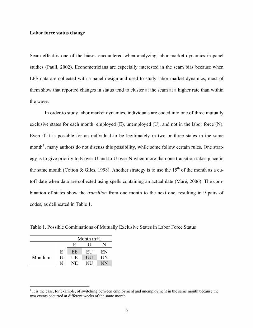
In order to study labor market dynamics, individuals are coded into one of three mutually
exclusive states for each month: employed (E), unemployed (U), and not in the labor force (N).
Even if it is possible for an individual to be legitimately in two or three states in the same
month1, many authors do not discuss this possibility, while some follow certain rules. One strat-
egy is to give priority to E over U and to U over N when more than one transition takes place in
the same month (Cotton & Giles, 1998). Another strategy is to use the 15th of the month as a cu-
toff date when data are collected using spells containing an actual date (Maré, 2006). The com-
bination of states show the transition from one month to the next one, resulting in 9 pairs of
codes, as delineated in Table 1.
Table 1. Possible Combinations of Mutually Exclusive States in Labor Force Status
Month m+1 E U N E EE EU EN Month m U UE UU UN N NE NU NN
1 It is the case, for example, of switching between employment and unemployment in the same month because the two events occurred at different weeks of the same month.
5

After each subject is classified in one state for each month, different rates can be com-
puted. In the LFS literature, the transitions on the diagonal of Table 1 (EE, UU, NN) are referred
to as stayers (stay rate) or non movers. These people maintain the same status from one month to
the next. The remaining six transitions are referred to as movers.
Seam effect for labor force status change in the SIPP
The first application of seam effect analysis to labor force status change in the SIPP (data collec-
tion every 4 months) dates to Martini (1989). He noticed an increase of the transitions rates for
the movers at the seam in comparison to the average of the three within-wave transitions for the
years 1984-85. Seam effects with SIPP labor force status changes in 1986 were subsequently
studied by Martini and Ryscavage (1991) finding a very similar pattern as before and, lastly, by
Nielsen and Gottschalck (2006) who concentrated the analysis for the years 1993, 1996 and
2001. The findings of these authors, who used very similar methods in computing the percentag-
es of transitions rates, are summarized in Table 2. We used the original idea of Kominski (1990)
of computing the ratio of seam vs. the average of within-wave transitions as a way to standardize
and compare different seam effects on the same scale. We then used Martini (1989), Martini &
Ryscavage (1991) and Nielsen and Gottschalck (2006) data and computed a within-wave average
for each of the movers transitions (month 1 to month 2; month 2 to month 3, and month 3 to
month 4) and used is as denominator while the average seam transition was used as nominator
thus creating a ratio2. In the absence of any seam bias this ratio should be close to 1.
2 Martini (1989) reports data for the year 1984 and 1985 for the non-institutional population 16 years and older (p. 390). Martini and Ryscavage (1991) report data for the year 1986 for the non-institutional population 16 years and older (p. 746). Lastly Nielsen and Gottschalck (2006) report data for the years 1993, 1996 and 2001 for the popula-tion 15 years and older (p. 29).
6
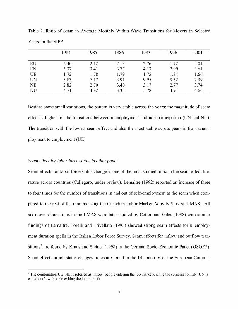
Table 2. Ratio of Seam to Average Monthly Within-Wave Transitions for Movers in Selected
Years for the SIPP
1984 1985 1986 1993 1996 2001
EU 2.40 2.12 2.13 2.76 1.72 2.01 EN 3.37 3.41 3.77 4.13 2.99 3.61 UE 1.72 1.78 1.79 1.75 1.34 1.66 UN 5.83 7.17 3.91 9.95 9.32 7.99 NE 2.82 2.70 3.40 3.17 2.77 3.74 NU 4.71 4.92 3.35 5.78 4.91 4.66
Besides some small variations, the pattern is very stable across the years: the magnitude of seam
effect is higher for the transitions between unemployment and non participation (UN and NU).
The transition with the lowest seam effect and also the most stable across years is from unem-
ployment to employment (UE).
Seam effect for labor force status in other panels
Seam effects for labor force status change is one of the most studied topic in the seam effect lite-
rature across countries (Callegaro, under review). Lemaître (1992) reported an increase of three
to four times for the number of transitions in and out of self-employment at the seam when com-
pared to the rest of the months using the Canadian Labor Market Activity Survey (LMAS). All
six movers transitions in the LMAS were later studied by Cotton and Giles (1998) with similar
findings of Lemaître. Torelli and Trivellato (1993) showed strong seam effects for unemploy-
ment duration spells in the Italian Labor Force Survey. Seam effects for inflow and outflow tran-
sitions3 are found by Kraus and Steiner (1998) in the German Socio-Economic Panel (GSOEP).
Seam effects in job status changes rates are found in the 14 countries of the European Commu-
3 The combination UE+NE is referred as inflow (people entering the job market), while the combination EN+UN is called outflow (people exiting the job market).
7

nity Household Panel (ECHP) (Fisher, Fouarge, Muffels, & Verma, 2002). A peculiarity of seam
effect for labor force transitions is that, due to the nature of the computation, an increase in the
movers rate corresponds to a decrease of the stayers because they are mutually exclusive states
(Carroll, 2006).
Kraus and Steiner (1998) were also able to compare the panel with register based data
confirming the fact that the transitions at the seam are an overestimation of the phenomena while
the transitions within the wave are an underestimation of the phenomena. This confirms previous
record-check studies on other variables (Marquis & Moore, 1989; Moore, Marquis, & Bogen,
1996).
Explanations for seam effects
There are many possible factors that are believed to be responsible for the seam effect phenome-
na. They can be classified into four categories: data processing, interview/coder inconsistencies,
memory issues and forms of satisficing. These four classes of causes frequently occur together
and the contribution of each of one depends on the kind of autobiographical event is being stu-
died. They have an impact on the types of errors that can occur during the interview: omission of
events (underreporting), and misclassification. The final effects on the estimates are within-wave
“constant wave response” and spurious transitions. This conceptual model explaining seam effect
is summarized in Table 3.
8

Table 3. Conceptual Model Explaining Seam Effects
Causes of error
Types of errors Effect on estimates
Data processing
⇒Omission Misclassification ⇒
Constant wave response Spurious transitions
Coder/interviewer inconsistencies Memory issues Satisficing
Burkhead and Coder (1985), Moore and Kasprzyk (1984), and Cotton and Giles (1998)
identify data keying error and edit issues as a possible source for seam effects in the SIPP panel.
It is also likely that procedures for assigning values for missing survey responses (imputation
strategies) are contributing to seam effects patterns (Lynn, Buck, Burton, Jäckle, & Laurie, 2005)
although no empirical research is presented by these authors.
Work done on the British Household Panel Survey (BHPS) (Halpin, 1998) showed that
coder inconsistencies (different coding of what was essentially the same job description) were
responsible for changes of the Standard Occupation Classification (SOC) code between waves
thus creating seam bias. Similar results were reported by Kalton, McMillen and Kasprzyk (1986)
and by Lynn & Sala (2006). Inconsistencies thus leading to seam effects are possible is there is a
change of interviewer between waves (Burkhead & Coder, 1985). Keying error can also create
spurious transitions, even if the same interviewer is present at both waves (Lynn, Buck, Burton,
Jäckle, & Laurie, 2005).
Another way of thinking about seam effects is to view them as the contrast between
memory for the most recent portion of the response period of the earlier wave, and memories for
the most remote portion of the response period of the later wave. The latter are likely to be an
estimate more than a direct recall (Rips, Conrad, & Fricker, 2003; Tourangeau, Rips, & Rasinski,
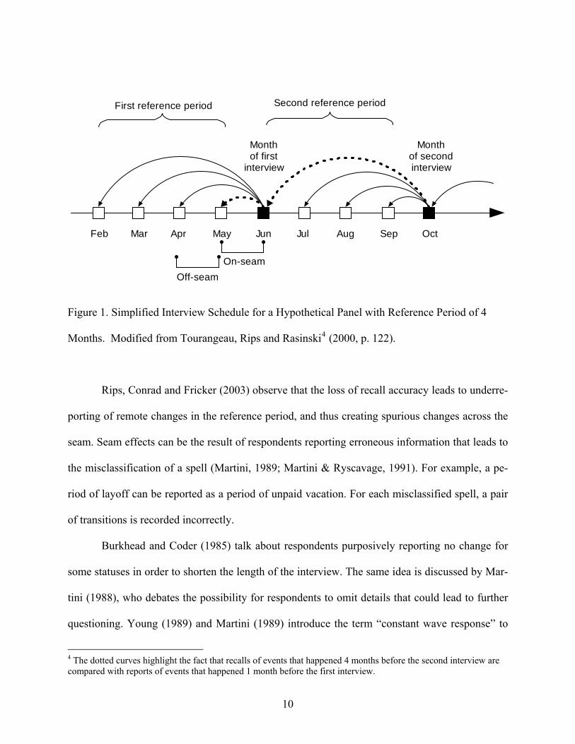
2000). Figure 1 exemplifies this concept.
9
Feb Mar Apr May Jun Jul Aug Sep Oct
First reference period Second reference period
Monthof first
interview
Monthof secondinterview
Off-seamOn-seam
Figure 1. Simplified Interview Schedule for a Hypothetical Panel with Reference Period of 4
Months. Modified from Tourangeau, Rips and Rasinski4 (2000, p. 122).
Rips, Conrad and Fricker (2003) observe that the loss of recall accuracy leads to underre-
porting of remote changes in the reference period, and thus creating spurious changes across the
seam. Seam effects can be the result of respondents reporting erroneous information that leads to
the misclassification of a spell (Martini, 1989; Martini & Ryscavage, 1991). For example, a pe-
riod of layoff can be reported as a period of unpaid vacation. For each misclassified spell, a pair
of transitions is recorded incorrectly.
Burkhead and Coder (1985) talk about respondents purposively reporting no change for
some statuses in order to shorten the length of the interview. The same idea is discussed by Mar-
tini (1988), who debates the possibility for respondents to omit details that could lead to further
questioning. Young (1989) and Martini (1989) introduce the term “constant wave response” to
4 The dotted curves highlight the fact that recalls of events that happened 4 months before the second interview are compared with reports of events that happened 1 month before the first interview.
10

define respondents who give an answer for earlier months in an interview period identical to the
other months that are asked about within the same interview. All these findings are now called
within-wave underreporting (Biemer & Lyberg, 2003, p. 139), a tendency that falls under the
concept of satisficing (Krosnick, Narayan, & Smith, 1996).
Constant wave response has its counterpart in the autobiographical memory literature. A
similar phenomena is called retrospective bias (Ross, 1989). Our memory for earlier periods of
our lives lacks details. In order to reconstruct them, we may extrapolate current characteristics
and apply them to the past. On one hand, if we expect that a characteristic did not change much,
we may infer that its value is identical to the present one. On the other hand, if we expect that a
characteristic changed quite a lot, we may exaggerate the amount of difference between the past
and the present. In the panel case, respondents may use their current status (easier to remember)
to estimate earlier values, but fail to adjust for changes in the more remote portions of the refer-
ence period.
In looking at the conceptual model explaining seam effect we can summarize the four
types of causes of seam effect as measurement error. Measurement errors are not specific to lon-
gitudinal surveys although their visibility as seam effect is (Lynn, 2005, p. 37). Seam effects
arise because of how the variables are computed. In looking for status changes generally from
one month to the next one, the transition computed between two waves suffer from the mea-
surement error of the first wave plus the measurement error of the second wave
(O’Muircheartaigh, 1996), thus showing the typical pattern of seam effect.
11
Reduction of seam effects
There are two main ways to reduce seam effects: the first one uses statistical adjustments after
the data are collected (Lynn, Buck, Burton, Jäckle, & Laurie, 2005) and the second one is based
on data collection strategies. In the second stream of research, involving data collection strate-
gies, solutions proposed include the use of dependent interviewing, the use of a calendar, keep-
ing the same interviewer in both waves, and the manipulation of question wording.
Dependent interviewing questions are classified as proactive and reactive (Brown, Hale,
& Michaud, 1998). In proactive dependent interviewing the respondents are asked questions they
did not answer in the previous wave, or reminded of previous responses. With reactive dependent
interviewing the information fed forward is used to carry out edit checks during the interview
(Jäckle, in press). Relevant to this paper is an experiment collecting labor history data involving
independent interviewing and proactive and reactive dependent interviewing carried out on a
subsample of the UK part of the European Community Household Panel (EHCP) (Jäckle &
Lynn, in press). The proactive dependent interviewing clearly reduced seam effects. For exam-
ple, transition rates [at the seam] for occupational status were reduced from 32% to 9% in the
proactive dependent interviewing group. The authors also maintain that proactive dependent in-
terviewing did not lead to underreporting of change since in the off-seam months the average
monthly transition rate was the same (2%) for all treatment groups.
A 32-month calendar was used as an aid for SIPP respondents in the Chicago region
(Kominski, 1990). After completion of the first face-to-face interview (wave 1), the interviewers
filled out a calendar with the information obtained from the standardized questionnaire. In the
second interview (wave 2) the interviewers handed the appropriate calendar to the respondents
12
prior to the start of the interview. During the interview the respondents were able to look at the
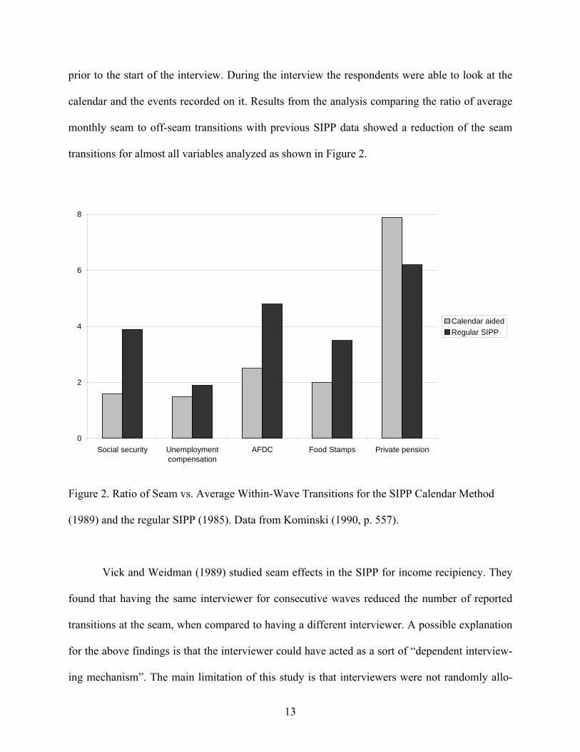
calendar and the events recorded on it. Results from the analysis comparing the ratio of average
monthly seam to off-seam transitions with previous SIPP data showed a reduction of the seam
transitions for almost all variables analyzed as shown in Figure 2.
0
2
4
6
8
Social security Unemploymentcompensation
AFDC Food Stamps Private pension
Calendar aidedRegular SIPP
Figure 2. Ratio of Seam vs. Average Within-Wave Transitions for the SIPP Calendar Method
(1989) and the regular SIPP (1985). Data from Kominski (1990, p. 557).
Vick and Weidman (1989) studied seam effects in the SIPP for income recipiency. They
found that having the same interviewer for consecutive waves reduced the number of reported
transitions at the seam, when compared to having a different interviewer. A possible explanation
for the above findings is that the interviewer could have acted as a sort of “dependent interview-
ing mechanism”. The main limitation of this study is that interviewers were not randomly allo-
13

cated to conditions, thus making more difficult in assessing the cause of an increase of seam ef-
fect when there is a switch.
Lastly, Rips, Conrad and Fricker (2003) reproduced a two-wave panel in laboratory set-
tings. During three different experiments they were able to reproduce the higher transitions at the
seam compared to the off seam weeks. The seam effect was a function of the difficulty of the
recall task, the length of the recall period, the grouping of questions by item or by reference pe-
riod (in this case, one week), and the order of retrieval. Seam effects enlarged with an increase of
the recall difficulty and length of recall. More importantly, grouping the questions by item in-
creased the constant wave response.
In summary, the common denominator of the methods that thus far have been proven ef-
fective in reducing seam effects is that they use different memory aids in helping the respondent
to retrieve information. Dependent interviewing, the use of a calendar, and having the same in-
terviewer give respondents more retrieval cues. In addition, grouping the questions by reference
period and not by item (Rips, Conrad, and Fricker, 2003) reduces satisficing behaviors and “in-
vites” the respondent to think more about the events.
Event History Calendar data collection methodology
The Event History Calendar (EHC) method is an emerging data collection technique that origi-
nates from the Life History Calendar (Freedman, Thornton, Camburn, Alwin, & Young-
DeMarco, 1988). An EHC interview is centered around a customized calendar that shows the
reference period under investigation (Axinn & Pearce, 2006). The calendar contains timelines for
different domains, for example work history, residence history, household composition and other
14

domains relevant to the topic of the study. Landmark events, such as holidays and birthdays are
noted in the timelines to aid respondent’s memory. The interviewer guides the respondent in fill-
ing out each timeline, starting with the landmark events and continuing down until all domains,
the focal points of the study, are completed. The process uses information and dates for each
completed domain to help the respondent correctly place other events in the appropriate time
frame. If, for example, the topic of the survey is unemployment history, respondents can use re-
trieval cues from their landmark events, residence history, and household composition to retrieve
the period in which they were unemployed. For instance, an unemployment period can happen
before a move to a new location or after a pregnancy. Interviewers follow a script where al-
though the order of the questions is suggested in advance, it can be adapted to the respondent’s
recollection process (Belli & Callegaro, in press-b).
Quality of data collected with EHC
When compared to CQ methods, EHCs have shown better data quality for retrospective reports
in terms of precision of the placement of events in time, and in terms of reducing underreporting
(Belli & Callegaro, in press-a).
Using validation data collected from the same respondents of the Panel Study of Income
Dynamics (PSID) years before, Belli, Shay, and Stafford (2001) showed that EHC reports were
more precise on moves, income, weeks unemployed, and weeks missing work resulting from
personal illness, the illness of another, or the combination of the two. In another study with PSID
respondents, this time using a computerized instrument and telephone interviews, Belli and col-
leagues (2007) collected retrospective reports with a reference period of up to 30 years. The res-
pondents were randomly assigned to either a standardized CATI interview or a computerized
15
EHC (C-EHC). The reports on social and economic variables of residential, marriage, cohabita-
tion, and work history were compared to the previous data collected from the same panel respon-
dents. The computerized EHC showed better overall data quality for cohabitation and work his-
tory; no difference was found for residence change and CQ showed better data only for marriage
history.
Hypotheses
The EHC interviewing method gives respondents more retrieval cues than those available in CQ.
EHC uses different memory retrieval strategies at once, such as the use of landmarks to anchor
events on the timeline. The flexible interviewing style of EHC allows the respondents to retrieve
the events in the order with which they feel more comfortable. Parallel probing gives the respon-
dents more retrieval cues because it takes advantage of the existence of interconnected thematic
and temporal pathways that can be used to remember specific events (Belli, 1998). The structure
of EHC, especially in its computerized version, highlights gaps in the timeline, alerting the inter-
viewer to probe for them thus possibly reducing item nonresponse and Don’t Know answers.
Another indication that supports the theoretical framework of this paper comes from the conclu-
sion of the seam effect paper by Rips and colleagues (2003, p. 552). They advance the hypothe-
sis that techniques such as EHC might be successful in reducing seam effects.
Seam effects are created by the manner in which panel data are collected. Since memo-
ries for the most recent portion of one response period are compared to memories of the earliest
portion of the next response period, it is likely than the latter are of less quality than the former.
Because the methodological studies conducted so far indicate that EHC leads to better retrospec-
16

tive data in terms of amount and precision of the recall, the recollection of the earliest portion of
the panel wave should be of better quality, thus reducing the spurious transitions that create seam
effects. Moreover, previous studies suggest that what drives seam effects is the inability to report
precisely when events happened. Since EHC interviewing aids respondents in locating the events
more precisely on the timeline, it is hypothesized that this data collection method should contri-
bute to the reduction of seam effects.
Data and methods
To test the hypotheses of this study, a concatenated dataset for the 1995-2005 waves of the Panel
Study of Income Dynamics was used (McGonagle & Schoeni, 2006; PSID staff, 2006). More
specifically, the dataset for waves 1995-2001 was obtained from the PSID data center5, an online
resource that enables the user to create a customized subset and companion documentation of the
public release data.
The variables used for the analyses are employment questions aimed to measure monthly
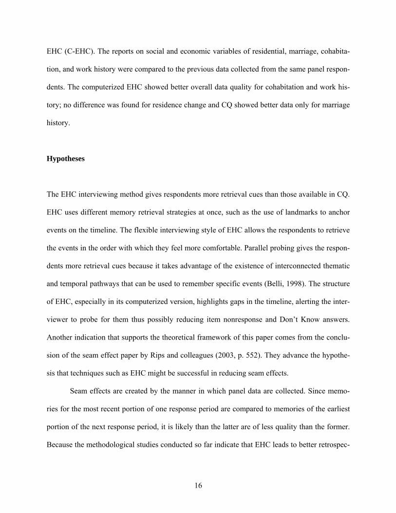
labor force status for the head and wife of the household. Figure 3 shows the waves used in the
analyses and the reference period of each wave.
5 http://simba.isr.umich.edu/
17
1994 1995 1996 1997 1998 1999 2000 2001 2002 2003 2004 2005
27 28 29 30 31 32 33Waves
Employmentquestionsregardingyears:
Seam
Seam
Seam
CQCQ EHCCQ EHCCQ
1 3 4
Seam
2
CQ
Seam
Seam
5 6
wws wws wws wws
Figure 3. PSID Waves used in the Analysis and Seam Points. Note: WWS = within-wave seam see description below.
Figure 3 also indicates the methodology of data collection, CQ or EHC, and seam points.
Seams 1 to 6 are the standard seams that occur when joining two waves of data collected at dif-
ferent years. The within-wave seam points (WWS) became available when the PSID started col-
leting data referring to a two year reference period in 1997 and are referred to the transitions be-
tween December of the first year (T −2) to January of the second year (T −1). In total, there are
ten seam points that will be the object of analysis. In the following paragraphs, the key methodo-
logical information about the dataset is reported. This will enable the reader to better understand
how the PSID measure labor status and who is answering those questions. More information
about the sampling design, response rates, and the survey content are found in McGonagle and
Schoeni (2006).
For the waves that are the object of this analysis (1995-2005) data were collected using
computer-assisted telephone interviewing. Beginning in 2003, a computer–assisted Event Histo-
ry Calendar instrument (Belli, 2003) was integrated with the current CATI instrument (Blaise)
and a major section of the questionnaire was administered that way.
The PSID collects information about family units (FU). The FU is defined as a group of
people living together as a family. Each FU has one and only one Head. In a married-couple
18

family the Head is considered to be the husband, unless the husband is severely disabled. The
person designated as Head can change overtime. The person living with the Head is defined as
Wife if legally married or “Wife” if cohabitant.
Unlike other panels, such as the GSOEP or the ECHP where all members 16 and older
are interviewed, PSID gathers information about all people residing in the FU but only one per-
son responds per household. Interviews are for the most part conducted with the Head or the
Wife (“Wife”).
PSID collects labor force status data only about the Head and the Wife of each house-
hold. The questionnaire contains separate questions for the Head and the Wife. Because only one
respondent is selected for the interview, the answers for the Head section could be self or proxy
depending on who is answering and vice versa. Because PSID attempts to interview either the
Head or the Wife, other household members are rarely used as proxy.
The questionnaire was the same for the waves 1995 to 1997 and 1999 - 2001 for events
happened the year before the interview, time T −1. Figure 4 shows a flow chart with the key va-
riables and the question wording used in the dataset. After the question about the employment
status (B/D39), detailed questions about each job (main and secondary) were asked such as a de-
scription of the occupation, duties, kind and name of business. Before asking about unemploy-
ment and out of labor force status, questions about work missed because of sickness, vacation
and strike were asked (B/D60-B/D/71).
19

HEAD/WIFEIS WORKING
NOWYes No
B/D39 In which months during(previous year) were you workingfor (employer) as your main job?
B/D72 Did you miss any work in(previous year) because you wereunemployed and looking for work
or temporary laid off?
YesB/D74a In which months were
you unemployed for at least oneweek?
B/D77 Were there any weeks in(previous year) when you didn'thave a job and were not looking
for one?
Yes
B/D77a Which months had atleast one week when you didn'thave a job and were not looking
for one?
No
Section C/EHead/wife is not working now
Same question wording for employment /unemployment and out of labor force but
different routing for people not working duringthe reference period
EMPLOYMENT
UNEMPLOYMENT
NOT IN THELABOR FORCE
B/D42 secondary main job
T-1 reference period
Figure 4. Questionnaire Flowchart for Labor Force Variables 1995-97 and 1999, 2001 T −1.
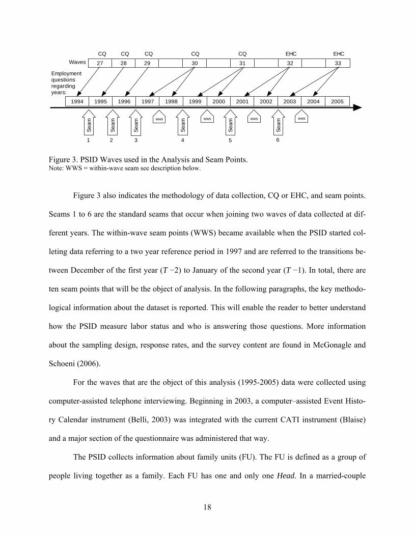
When the PSID switched to a two-year data collection in 1997, the questions about the
job status referring to two years before the interview (T −2) were asked in a more simplified way,
and not consecutively after the question referring to time T −1 Moreover, the “not in the labor
force” question was not requested for T −2.
20
R25/R32 Did you (head ofwife) work at a job of business
at any time during(1999)?
Yes R28/R35 During whichmonths was that?
No
R30/R37 Were there any months in(1999) in which you were
unemployed and looking for work forat least one week?
EMPLOYMENT
UNEMPLOYMENT
Yes Which months werethose?
No
Figure 5. Questionnaire Flowchart for Labor Force Variables 1999 and 2001 T −2
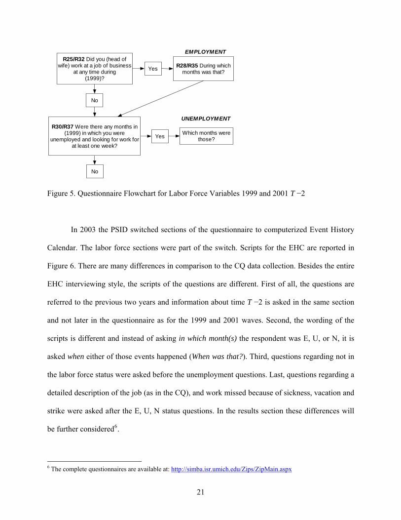
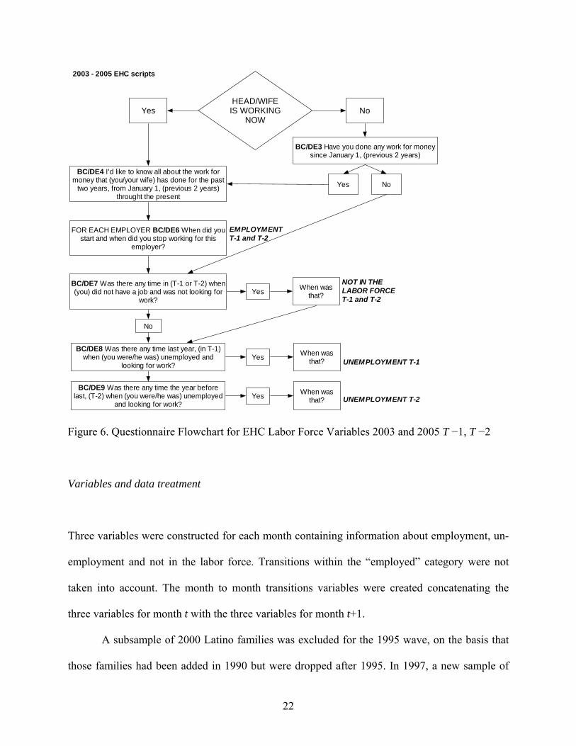
In 2003 the PSID switched sections of the questionnaire to computerized Event History
Calendar. The labor force sections were part of the switch. Scripts for the EHC are reported in
Figure 6. There are many differences in comparison to the CQ data collection. Besides the entire
EHC interviewing style, the scripts of the questions are different. First of all, the questions are
referred to the previous two years and information about time T −2 is asked in the same section
and not later in the questionnaire as for the 1999 and 2001 waves. Second, the wording of the
scripts is different and instead of asking in which month(s) the respondent was E, U, or N, it is
asked when either of those events happened (When was that?). Third, questions regarding not in
the labor force status were asked before the unemployment questions. Last, questions regarding a
detailed description of the job (as in the CQ), and work missed because of sickness, vacation and
strike were asked after the E, U, N status questions. In the results section these differences will
be further considered6.
6 The complete questionnaires are available at: http://simba.isr.umich.edu/Zips/ZipMain.aspx
21
HEAD/WIFEIS WORKING
NOWYes No
EMPLOYMENTT-1 and T-2
UNEMPLOYMENT T-1
NOT IN THELABOR FORCET-1 and T-2
BC/DE3 Have you done any work for moneysince January 1, (previous 2 years)
BC/DE4 I'd like to know all about the work formoney that (you/your wife) has done for the past
two years, from January 1, (previous 2 years)throught the present
FOR EACH EMPLOYER BC/DE6 When did youstart and when did you stop working for this
employer?
Yes No
BC/DE7 Was there any time in (T-1 or T-2) when(you) did not have a job and was not looking for
work?Yes When was
that?
BC/DE8 Was there any time last year, (in T-1)when (you were/he was) unemployed and
looking for work?Yes When was
that?
No
2003 - 2005 EHC scripts
UNEMPLOYMENT T-2BC/DE9 Was there any time the year before
last, (T-2) when (you were/he was) unemployedand looking for work?
Yes When wasthat?
Figure 6. Questionnaire Flowchart for EHC Labor Force Variables 2003 and 2005 T −1, T −2
Variables and data treatment
Three variables were constructed for each month containing information about employment, un-
employment and not in the labor force. Transitions within the “employed” category were not
taken into account. The month to month transitions variables were created concatenating the
three variables for month t with the three variables for month t+1.
A subsample of 2000 Latino families was excluded for the 1995 wave, on the basis that
those families had been added in 1990 but were dropped after 1995. In 1997, a new sample of
22
immigrants was introduced in the study, starting with 441 families in 1997 and reaching 511 in
1999. This sample was dropped from the analysis to keep consistent with the decision to drop the
previous sample of Latinos. In 1997 the PSID also reduced the core sample from the nearly
8,500 families in 1996 to approximately 6,168 in 1997 (McGonagle & Schoeni, 2006).
Although it is possible that more that one status is legitimately present for each given
month (e.g. being employed and unemployed in the same month), the analysis is performed on
the net transitions (i.e. ignoring multiple transitions in the same month because unclassifiable)7.
The focus is then on the nine possible transitions that were delineated in Table 1. Those consist
of a 1995-2005 average of 97.8% (SD=1.7) among all possible transitions.
Because in the 1999 and 2001 waves a question about “not in the labor force status” (N)
was not asked for time T −2, an imputation strategy8 has been applied in order to obtain the N
variable necessary to compute the transitions at the seam. Results from the CQ 1999 and 2001
T −2 transitions should be interpreted with cautiousness.
Lastly, in order to make meaningful comparison across seam points, the age at the seam
has to be investigated. If for example the panel is aging, it is more likely to have more transitions
employed – out of labor force, at later waves. The PSID following and eligibility rules however
avoid that. In fact the mean age for the six seam points is not really moving in any meaningful
direction for the 10 years object of investigation (around 43.5 years of age). More details on the
data analysis and treatment are found in Callegaro (2007).
7 The problem with multiple transitions in the same month is that it is not possible to assess the temporal order. If somebody reports to be employed and unemployed in the same month, there is no way to know if this person was employed and then unemployed or unemployed and then employed. For this reason, multiple transition within a month are unclassifiable. 8 A “N” status was imputed for the months in which the respondent reported to be retired. If the panel participant reported to be working in time T-2, the N status was imputed in the month where the respondent was not working and was not looking for a job.
23
24
Primary findings
When reporting results, the names of the variables will refer to the reference period investigated
in each wave, and not to the year in which the data were collected. This will simplify the inter-
pretation and clarify the seam points (see Figure 3).
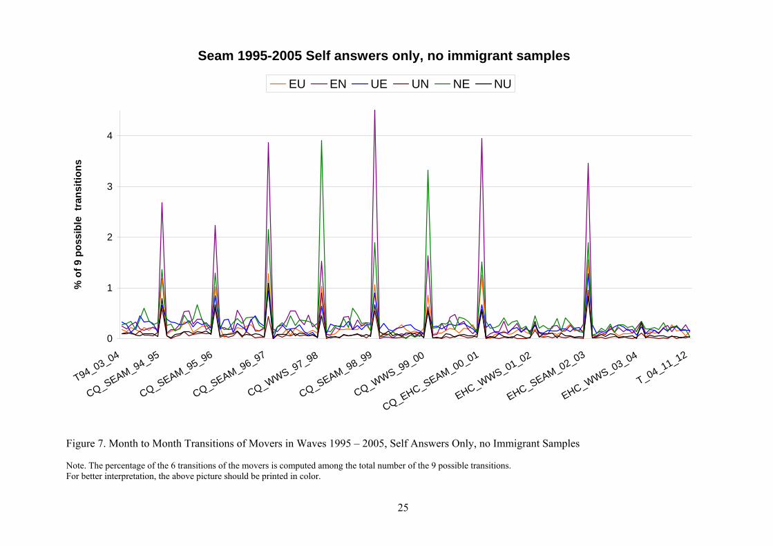
Figure 7 is created plotting for each pair of months the percentage of movers for the six
categories in which status changes could take place (EU, EN, UE, UN, NE, NU) among all the
stayers and movers nine classifiable status changes (see Table 1). For example the EN percen-
tage for the transition point January to February is obtained dividing the number of reports being
E in January and N in February (EN) divided by the reports (EE + EU + EN+ UE, + UU + UN +
NE + NU +NN)*100. Multiple status changes per month (unclassifiable) are not reported.
Figure 7 shows six interesting phenomena. First of all, the PSID is not exempt of seam
effect for labor force data in the latest seven waves. Seam effect was first found in the PSID for
variables such as unemployment compensations and food stamp recipiency (Hill, 1987). In order
to test if the number of transitions at the seam (from December to January) is statistically differ-
ent from the number November-December transitions before that seam, a test of marginal homo-
geneity was used9 (Agresti, 2002). The test shows that all seam points are different from the No-
vember-December transition at a statistical significant level (.01).
9 Because the answers of panel respondents are dependent, the appropriate test for two dependent samples (paired) with a multinomial outcome for ordinal data (9 possible transitions) is the test of Marginal Homogeneity. The null hypothesis states that the row and column marginal response distribution of the respondents to the seam and the No-vember-December transition will be the same. The alternative hypothesis states that for at least one transition, the marginal distribution of the seam will not be equal to the marginal distribution of the November-December transi-tion. The test is performed only with the subjects whose answers are present in both transitions. The test is an exten-sion of the McNemar test for binary responses.
Seam 1995-2005 Self answers only, no immigrant samples
0
1
2
3
4
T94_03_04
CQ_SEAM_94_95
CQ_SEAM_95_96
CQ_SEAM_96_97
CQ_WWS_97_98
CQ_SEAM_98_99
CQ_WWS_99_00
CQ_EHC_SEAM_00_01
EHC_WWS_01_02
EHC_SEAM_02_03
EHC_WWS_03_04
T_04_11_12
% o
f 9 p
ossi
ble
tran
sitio
nsEU EN UE UN NE NU
Figure 7. Month to Month Transitions of Movers in Waves 1995 – 2005, Self Answers Only, no Immigrant Samples Note. The percentage of the 6 transitions of the movers is computed among the total number of the 9 possible transitions. For better interpretation, the above picture should be printed in color.
25
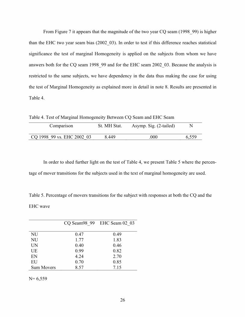
From Figure 7 it appears that the magnitude of the two year CQ seam (1998_99) is higher
than the EHC two year seam bias (2002_03). In order to test if this difference reaches statistical
significance the test of marginal Homogeneity is applied on the subjects from whom we have
answers both for the CQ seam 1998_99 and for the EHC seam 2002_03. Because the analysis is
restricted to the same subjects, we have dependency in the data thus making the case for using
the test of Marginal Homogeneity as explained more in detail in note 8. Results are presented in
Table 4.
Table 4. Test of Marginal Homogeneity Between CQ Seam and EHC Seam
Comparison St. MH Stat. Asymp. Sig. (2-tailed) N
CQ 1998_99 vs. EHC 2002_03 8.449 .000 6,559
In order to shed further light on the test of Table 4, we present Table 5 where the percen-
tage of mover transitions for the subjects used in the text of marginal homogeneity are used.
Table 5. Percentage of movers transitions for the subject with responses at both the CQ and the
EHC wave
CQ Seam98_99 EHC Seam 02_03
NU 0.47 0.49 NU 1.77 1.83 UN 0.40 0.46 UE 0.99 0.82 EN 4.24 2.70 EU 0.70 0.85 Sum Movers 8.57 7.15
N= 6,559
26
Results from the Table 4 and 5 support the initial hypothesis: EHC data collection me-
thodology reduced the seam effect in comparison to the CQ. In comparing CQ and EHC seam
points we have to remember the following. Because the test of Marginal Homogeneity uses the
same subjects across waves, the status changes of the EHC seam points belong to subjects
slightly older than when the measurement was computed in the CQ. This might be a potential
confounding factor because older subjects can have different status changes patterns.
Third, a previously undocumented phenomenon appears in the data: the presence of with-
in-wave seam effects (e.g. CQ_WWS_97_98 in Figure 7; that is, there are higher transition rates
between December of the first year and January of the second year of the reference period (mar-
ginal homogeneity test significant) than in November and December of the first year, or January
and February of the second year. The effects seem surprising at first, because the data were col-
lected during the same interview. On the other hand, T −2 questions were asked separately from
T −1 job status questions, 40 minutes later in the questionnaire, and in a more simplified way.
The simplification of the questionnaire is more likely the strongest contribution to the within-
wave seam effect because of the limited retrieval cues offered to the respondents in the CQ data
collection. The within-wave EHC seams (e.g. EHC_WWS_01_02) are almost nonexistent (mar-
ginal homogeneity test not significant). In fact questions were asked concurrently referring to the
two year reference period for E and N status, and for T −1 and then T −2 for the N status (see
Figure 6).
The fourth finding is that EN (purple line) and NE (green line) transitions are more sensi-
tive to seam effect. This is an indication of the difficulty for the respondent to separate the con-
cepts of “unemployment” from “not in the labor force” that, although clear in the official defini-
tion, have been proven to be of not easy comprehension for the respondent (Campanelli, Martin,
27

& Rothgeb, 1991). Another cause could be the fact that it is more difficult to remember a non
event (was there any time when you were unemployed and not looking for a job) than an event.
Fifth, based on the above hypothesis, it is expected that the one year recall period CQ
seam point would be of lower magnitude than the two year recall period seam point. In other
words we are expecting a statically significant difference between the one year CQ and the two
years seam points. In order to test the above hypothesis the first seam point 1994_95 will be
compared with the two year seam points starting from the 1998_99 CQ. Because the two year
seam points are far away in time from the 1994_95 seam, it is not fair to consider only the same
cases present at both waves because the same subjects are getting older thus having a different
job history pattern than when they were younger. The test will then consider the two samples of
each seam point as independent. Table 6 presents results of three Chi square comparisons among
the 1994_95 one year recall period and the three seam points with a two year recall period.
Table 6. Chi Square Test Between One Year Seam Point and Two Year Seam Points
Comparison X 2 p Df
1 year CQ 1994_95 vs. 2 year CQ 1998_99 117.01 .000 8 1 year CQ 1994_95 vs. 2 year CQ_EHC 2000_01 124.81 .000 8 1 year CQ 1994_95 vs. 2 year EHC 2002_03 155.84 .000 8
Each comparison reaches statistical significance, meaning that the one year seem bias is
always lower than any two year seam bias. These results provide further evidence to the initial
finding by Hill (1987) that increasing the recall period increases the amount of seam bias. Hill
used two panels (PSID and SIPP) to come to this conclusion while with this dataset it was possi-
ble to test the above hypothesis using the same panel thus making the conclusion stronger.
Last, the EHC within-wave transitions are smoother than the CQ transitions. It is difficult
to pinpoint the exact cause for the smoother data because of all the changes in question wording
28

and data collection. It is however worth to note that the nature of the EHC data collection and its
calendar feature “invites” the respondent to be more consistent and to fill gaps in the timeline.
This characteristic can be the cause of the smoothness of the within-wave transitions in the EHC
waves.
Secondary findings
In this section of the paper we explore if and how personal variables (e.g. age, sex, education,
race) or design variables (e.g. self or proxy answer, time lag between the interview and the refer-
ence period, having the same interviewer at both waves) have an effect on the magnitude of seam
bias.
Because validation data are not available for the PSID, the strategy used in the forthcom-
ing analyses is the following: as best approximation to validation data, all movers transitions at
the seam are taken “as seam bias”. The reasoning behind is that even if we know that some
people had a legitimate transition at the seam, we also know that the majority of transitions at the
seam are error. A simple calculation can give us an idea of the magnitude of this error. By sum-
ming up the six movers transitions at the seam and comparing them with the sum of the previous
November-December movers transitions we can compare the percentage of error at the seam, i.e.
the percentage of spurious transitions. The November December transition is considered the
most precise report for each wave because it is the closest to the interview date and for this rea-
son less prone to memory decay. The November December transition is also the best reference
point to compare the seam transition because closest in time and less sensitive to seasonal effects
in the job market. Table 7 provides these calculations for two seam points that will be object of
29
further analysis. For table 7 we used all available subjects from whom we have responses for the
November December transition and the following seam.
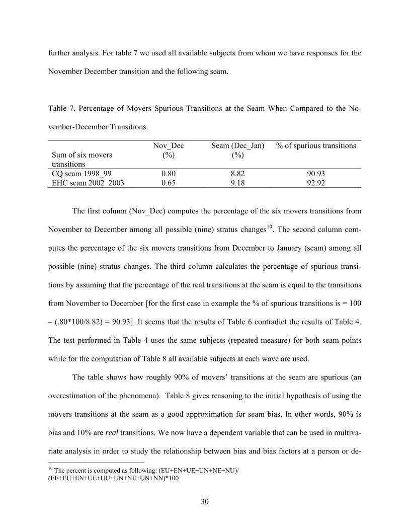
Table 7. Percentage of Movers Spurious Transitions at the Seam When Compared to the No-
vember-December Transitions.
Sum of six movers transitions
Nov_Dec (%)
Seam (Dec_Jan) (%)
% of spurious transitions
CQ seam 1998_99 0.80 8.82 90.93 EHC seam 2002_2003 0.65 9.18 92.92
The first column (Nov_Dec) computes the percentage of the six movers transitions from
November to December among all possible (nine) stratus changes10. The second column com-
putes the percentage of the six movers transitions from December to January (seam) among all
possible (nine) stratus changes. The third column calculates the percentage of spurious transi-
tions by assuming that the percentage of the real transitions at the seam is equal to the transitions
from November to December [for the first case in example the % of spurious transitions is = 100
– (.80*100/8.82) = 90.93]. It seems that the results of Table 6 contradict the results of Table 4.
The test performed in Table 4 uses the same subjects (repeated measure) for both seam points
while for the computation of Table 8 all available subjects at each wave are used.
The table shows how roughly 90% of movers’ transitions at the seam are spurious (an
overestimation of the phenomena). Table 8 gives reasoning to the initial hypothesis of using the
movers transitions at the seam as a good approximation for seam bias. In other words, 90% is
bias and 10% are real transitions. We now have a dependent variable that can be used in multiva-
riate analysis in order to study the relationship between bias and bias factors at a person or de- 10 The percent is computed as following: (EU+EN+UE+UN+NE+NU)/ (EE+EU+EN+UE+UU+UN+NE+UN+NN)*100
30
sign level. Another way to look at the issue is to think about a baseline of error common to each
seam point.
In order to find out what variables are effecting the error at the seam two exploratory lo-
gistic regressions are performed on seam 4 (CQ1998-99, two year reference period) and seam 6
(EHC 2002-03, two year reference period). Logistic regression appears to be the best fit for the
kind of data in hand. In comparison to other techniques, such as discriminant function, it does
not have assumptions about the distributions of the predictor variables, the predictors do not have
to be normally distributed, linearly related, or of equal variance within each group (Tabachnick
& Fidell, 2001 p. 517).
Description of the dependent variable
The dependent variable will be the presence of seam effect or not (group membership 1, 0). In
order to compute group membership each answer will be classified at each seam according to the
following rules: people reporting a transition or movers (EU, EN, UE, UN, NE, NU) will be clas-
sified as belonging to the seam effect group (coded as 1). People not reporting a transition or
stayers (EE, UU, NN) will belong to the no change group (coded as 0). Predictor variables, their
categories and measurement level are delineated in Table 8. The selection of the above variables
is dictated by the knowledge gained from studies on factors affecting the magnitude of seam ef-
fect plus some other hypothesis matured during the course of this investigation.
31
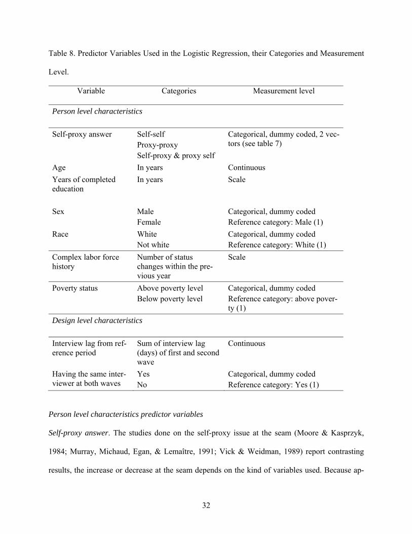
Table 8. Predictor Variables Used in the Logistic Regression, their Categories and Measurement
Level.
Variable Categories Measurement level
Person level characteristics Self-proxy answer Self-self
Proxy-proxy Self-proxy & proxy self
Categorical, dummy coded, 2 vec-tors (see table 7)
Age In years Continuous Years of completed education
In years Scale
Sex Male Female
Categorical, dummy coded Reference category: Male (1)
Race White Not white
Categorical, dummy coded Reference category: White (1)
Complex labor force history
Number of status changes within the pre-vious year
Scale
Poverty status Above poverty level Below poverty level
Categorical, dummy coded Reference category: above pover-ty (1)
Design level characteristics Interview lag from ref-erence period
Sum of interview lag (days) of first and second wave
Continuous
Having the same inter-viewer at both waves
Yes No
Categorical, dummy coded Reference category: Yes (1)
Person level characteristics predictor variables
Self-proxy answer. The studies done on the self-proxy issue at the seam (Moore & Kasprzyk,
1984; Murray, Michaud, Egan, & Lemaître, 1991; Vick & Weidman, 1989) report contrasting
results, the increase or decrease at the seam depends on the kind of variables used. Because ap-
32

proximately 40% of answers in the PSID are proxy (including the combinations proxy self- self-
proxy) the variable self-proxy appears to be an important predictor to be included in the explora-
tory models. The reader should keep in mind that in our case the proxy is either the Head or the
Wife, and that receiving the status of Wife is dependent for either being legally married or from
cohabitating for at least one year. In order to include in the model the variable self-proxy answer
(categorical) a transformation is necessary. A categorical variable is coded into N-1 number of
levels dummy vectors (Pedhazur, 1997). These new vectors need to be independent (orthogonal)
of each other. In this case, because self-proxy and proxy-self were combined due to the small
sample size, we have 3-1=2 new dummy variables as showed in Table 9. The group object of
comparison should be the group with the highest frequency i.e. Self-Self (00).
Table 9. Dummy Coding of the Predictor Variable Self-Proxy Status
Group PSSP (SS) PP (SS)
Self-Self 0 0 Self-proxy & proxy-self 1 0 Proxy-proxy 0 1
Self-proxy answers at the seam also present a potential confounding factor. In a house-
hold where Head and Wife are present, it is possible that there is a correlation of error between
the self and the proxy answers. If this is the case, self answers from a single Head household
could not be treated in the same way as self answers from a Head – Wife household. For this rea-
son, a correlation between self and proxy answer [classified as staying (EE, UU, NN) or moving
(EU, EN, UE, UN, NE, NU] was computed for households in which answers for the Head and
the Wife were present. Because at the seam there might a switch between self and proxy an-
33

swers, two Pearson’s r correlations were computed11, the first one is where there is no switch of
respondents at the seam (self self or proxy proxy), the second one when there is a switch (self
proxy and proxy self). Results from the correlations are reported in Table 10. Values of r for
both EHC and CQ indicate a very small but significant correlation between self and proxy an-
swers when the respondent is the same across waves. The correlation between self and proxy an-
swers when there is a switch of respondent between waves is not statistically significant. These
results provide evidence in favor of treating answers for single household together with answers
from a Head-Wife household.
Table 10. Pearson r Correlations Between Self and Proxy Answers from the Same Household
Seam r Approx sign.
N
CQ 1998_99 Same respondent in both waves .106 .000 2,386 CQ 1998_99 Switch of respondent between waves -.010 .908 135
EHC 2002_03 Same respondent in both waves .042 .031 2,689 EHC 2002_03 Switch of respondent between waves -.022 .783 159
Table 10 suggests an even smaller correlation for EHC answers in comparison to CQ an-
swers among the same respondents across waves. A possible research question would be to test if
the EHC correlation is significantly lower than the CQ correlation. Due to the dependency of the
correlations because most of the same subjects are respondents in the two waves, it is necessary
to use a test that accounts for dependent correlations (Chen & Popovich, 2002). Steiger (1980)
proposes using Dunn and Clark (1969) z test formula to test for the difference between two de-
11 Strictly speaking, the Phi (φ) coefficient should be used when computing correlation between two dichotomous
variables. However the phi coefficient and Pearson's r are algebraically equivalent when computed on dichotomous
variables.
34
pendent correlations with zero elements in common for samples > 20. The results were then ob-
tained using Depcor, a Fortran 77 program for comparing dependent correlations (Silver & Hitt-
ner, 2006). Due to the small sample size of the CQ and EHC correlation when the respondents
are switching between waves (line two and four of Table 11), the Dunn and Clark z test was not
computed. When comparing the two correlations between CQ (.106) and EHC (.042) the ob-
tained Dunn and Clark12 z is of 2.097 with p value of 0.018. This means that the correlation of
error between self and proxy responses in the CQ is higher than for the EHC.
The very low correlation of error between self and proxy answers speaks in favor in ac-
cepting the logistic regression assumption of independence of errors (responses of different cases
are independent of each other).
Age. Age was found to amplify inconsistencies of reports at the seam by Hill (1987) and
Jäckle and Lynn (in press) thus creating higher seam bias. Age in the PSID is measured in num-
ber of years. Respondents become eligible to be interview when they form an economically in-
dependent household. The range of age goes from 15 years old to 99 with a mean around 43
years old.
Years of completed education. This variable was included as a surrogate for cognitive
capacity in order to test if that has an effect on the seam bias. The variable is measured using the
completed grade in school where 17 is the maximum and indicates at least some post-graduate
work.
Sex. Although sex was not found to be a predictor of seam bias in the previous studies, it
is considered important to be included in the model as a control variable. Male is the reference
category coded as 1.
12 Since the formula asks for only one sample size and the N was different for any pair of correlation due to attrition
and item nonresponse, the harmonic mean of 2,127 was used.
35
Race. Race was found to have an effect at the seam by Hill (1987). African Americans
were found to be more likely to provide higher inconsistencies at the seam than non African
American, controlling for education, sex, age and income. Race is dummy coded in the analysis
where White is the reference category coded as 1.
Complex labor force history. This variable is hypothesized to have a strong impact on
the model. The hypothesis is that at an increase of job changes, there is an increased likelihood to
report a spurious transition at the seam. People with complicated job histories, in and out of the
job market, have more chances to make more errors than somebody who holds a steady job for
the entire reference period. Source monitoring and telescoping, for example, can create spurious
transitions. Hill (1987) found a statistically significant negative relationship between the number
of months with the current employer and amplifying inconsistencies at the seam. Complex labor
force history is measured counting the number of status change during the year before the seam
(Time T-1). In this case people reporting multiple changes within a month (the previously men-
tioned unclassifiable cases) are included in the model because it is a strong indication of com-
plexity of job status.
Poverty status. Poverty status can have an effect on entering and exiting the labor market.
The poverty variable was created as the following: Income need=Total family income / Census
income to needs. Total family income refers to tax year. This variable is the sum of five va-
riables: taxable income of head and wife, transfer income of head and wife, taxable income of
other family unit members, transfer income of other family unit members, and Social Security
income. The variable can contain negative values indicating a net loss. Negative values for in-
come were brought to 1 dollar (very few cases).
36

Census income to needs referring to 1998 was taken from the Census poverty threshold
website (U.S. Census Bureau, 2007a). The threshold values are based on family size, the number
of persons in the family under age 18, and the age of the householder. This variable has been ad-
justed for changes in family composition during 1999 so that it matches part-year incomes in-
cluded in the total family money income. The same strategy was used for year 2002 (U.S. Cen-
sus Bureau, 2007b). Then two new variables were thus created: POVERTY88 and POVERTY02
as the following: if the ratio is < 1 then the family is in poverty. The new recoded variables were
recoded as 0 or 1, where 0 means below poverty and 1 above poverty.
Design level characteristics predictor variables
Interview lag from reference period. Because PSID interviews starts in February and
ends in November, it is plausible to think that people interviewed in November might have high-
er seam effect than people interviewed in February for the first and the second wave. This varia-
ble is measured summing up the number of elapsed days from the first interview to December 1st
of the first wave plus the number of days elapsed from the second interview to January 1st of the
second wave.
Having the same interviewer. Wick and Weidman (1989) found that having the same in-
terviewer at both waves decreased seam effect in the SIPP panel. The SIPP was a face to face
data collection with interviews approximately every four months. In the PSID the interviews are
by phone and now every two years. For this reason, the initial hypothesis that having the same
interviewer could potentially reduce seam effect appears difficult to be verified but it is worth
exploring the possibility of it. The variable is measured using interviewers ID where in the case
37
of match a value of 1 is assigned. Unfortunately in 2005 the interviewers’ ID numbering system
changed, thus rendering the computation impracticable for the EHC seam.
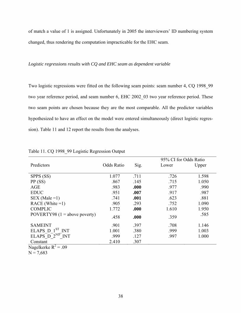
Logistic regressions results with CQ and EHC seam as dependent variable
Two logistic regressions were fitted on the following seam points: seam number 4, CQ 1998_99
two year reference period, and seam number 6, EHC 2002_03 two year reference period. These
two seam points are chosen because they are the most comparable. All the predictor variables
hypothesized to have an effect on the model were entered simultaneously (direct logistic regres-
sion). Table 11 and 12 report the results from the analyses.
Table 11. CQ 1998_99 Logistic Regression Output
95% CI for Odds Ratio Predictors Odds Ratio Sig. Lower Upper
SPPS (SS) 1.077 .711 .726 1.598 PP (SS) .867 .145 .715 1.050 AGE .983 .000 .977 .990 EDUC .951 .007 .917 .987 SEX (Male =1) .741 .001 .623 .881 RACE (White =1) .905 .293 .752 1.090 COMPLIC 1.772 .000 1.610 1.950 POVERTY98 (1 = above poverty) .458 .000 .359 .585
SAMEINT .901 .397 .708 1.146 ELAPS_D_1ST_INT 1.001 .380 .999 1.003 ELAPS_D_2ND_INT .999 .127 .997 1.000 Constant 2.410 .307
Nagelkerke R2 = .09 N = 7,683
38

Table 12. EHC 2002_03 Logistic Regression Output
95% CI for Odds Ratio Predictors Odds Ratio Sig. Lower Upper
SPPS (SS) 1.198 .345 .824 1.743 PP (SS) 1.021 .824 .848 1.230 AGE .985 .000 .979 .991 EDUC .931 .000 .898 .965 SEX (Male=1) .717 .000 .607 .848 RACE (White=1) .757 .001 .639 .897 COMPLIC 1.796 .000 1.670 1.932 POVERTY02 (1 = above poverty) .411 .000 .330 .510
ELAPS_D_1ST_INT 1.001 .486 .999 1.002 ELAPS_D_2ND_INT 1.002 .088 1.000 1.003 Constant .262 .109
Nagelkerke R2 = .136 N = 8,212
The design level characteristic variables do not help in the fit of the model. The inter-
viewer lag is maybe too long anyway. Having the same interviewer does not help either. This
might be the case that the lag between the two interviews is too long, that the interviews were
done on the phone, and the fact that because only 13.6% of interviewers were the same for the
CQ seam 1998_99 there is not enough statistical power to detect any differences.
The two models provide very close results for the predictors. The CQ model accounts for
about 9% of the variance while the EHC for about 13.6%. Although these results are not impres-
sive, the reader should be reminded that the dependent variable contains some error because it
was not possible to distinguish between real transitions and spurious transitions.
An increase in age slightly decreases the odds of having seam bias. These results seem to
contradict previous research (Hill, 1987; Jäckle & Lynn, in press). On the other hand because
this model controls for complex labor force histories, an increase in age can just mean that older
39
people are more likely to have stable jobs and be more likely to be stayers for the entire year.
This is even truer when people retire.
Education can be seen as a surrogate measure of cognitive capacity and it goes in the ex-
pected direction, people with higher education have lower seam bias. Higher education can also
mean having more stable jobs.
The odds to show bias are 1.4 times lower for man than for women in both models
(1/0.741 for CQ and 1/0.717 for EHC). Non-Whites are 1.3 (=1/0.757) times more likely to show
seam bias than Whites. In the CQ model race does not reach statistical significance. Because the
model is controlled for the number of labor force transitions, age, and education, these results
regarding race are not easy to explain. Moreover, in a previous analysis where the poverty level
was not entered we had statistically significant results for race for both CQ and EHC (Callegaro,
2007, p. 102). More research is needed on this regard, possibly employing datasets with valida-
tion data.
People with more job status changes within the wave are more likely to show bias at the
seam. Because complicated life history is measured counting the number of transitions within the
wave, we can interpret the odds ratio of 1.8 for both CQ and EHC to signify that an increase of 1
on the complicated like history measure doubles the odds of showing seam bias. This is the vari-
able with the highest odds ratios. The more changes in job status during the year, the more
chances to make a mistake and report a transition at the seam. It is also true that the more
changes during the year, the more likely is to change at the seam.
The self-proxy variable is a predictor that does not seem to have an impact on seam bias
when controlling for everything else.
40
The poverty has the second biggest impact on the model after complex labor force histo-
ry. People below the poverty threshold are 2.2 (CQ: 1/0.458) and 2.4 (EHC: 1/0.411) times more
likely than people above the poverty line to show bias at the seam.
Study limitations
Although in the analysis it was possible to control for some confounding variables such as the
immigrant sample and the self/proxy answers, others remained present: the comparison of EHC
and CQ seams is confounded by the wording of the questionnaire. In the CQ case, people were
asked about employment, unemployment and out of labor force with months as response options
(i.e. in which months during [previous year] were you working for [name of employer]). In the
EHC case, the question wording required more precision in remembering the job history (e.g.
when did you start and stop working for [name of employer]) than the CQ version (e.g. in which
months were you working for…).
In addition, data might be affected by order effect; in the previous discussion of the CQ
and EHC questionnaires (Figures 4-6) it was noticed how the N question was asked before the U
question in the EHC and the other way around in the CQ. Also, in the CQ, specific questions
about the job and time missed for sickness, vacation and strike were asked after the employment
section while in the EHC they were asked after the entire E, N, U section. Asking these questions
after the timing of E, U, and N could have given less retrieval cues to the respondents although in
the EHC the interview is more flexible and it is easier to go back and forth on the timelines mak-
ing adjustments as they come up. All these differences in question wording make the comparison
between CQ and EHC problematic at best. The present study does not include a control group
41
where the same question wording was asked in CQ mode or EHC mode. In this ideal case the net
contribution of the EHC data collection methodology could have been studied with no confound-
ing factors.
Conclusions
Seam effects have been observed in different panels, with different reference periods and with
different modes of data collection. All the papers written so far analyze data that were collected
with a standardized conventional questionnaire. This study investigates the trend of the magni-
tude of seam effects in labor force data in the PSID from a data user point of view. The data pro-
vide further evidence of previous seam effect findings, specifically that seam effect intensifies at
an increase of the reference period between two waves. The EHC seam effect was found of
slightly less magnitude than the CQ seam effect.
The analysis showed a new phenomenon, the “within-wave seam effect”, found when the
PSID moved to a two year reference period. The explanation for this effect might lie in the de-
sign of the CQ questionnaire. In fact, questions about labor force status for time T −1 were asked
at the beginning of the interview and those regarding T −2 took place 40 minutes later and in a
much more simplified way. The within-wave seam suggests how questionnaire design can create
seam effects during the same data collection period. Supporting this idea, when the questionnaire
was changed in the EHC waves, the within-wave seam disappeared despite the fact that even
with the EHC, any unemployment experienced in the most recent year was asked separately, and
before, any unemployment experienced in the more remote year.
42

Labor force surveys in panel data contain many sources of measurement error (Bound,
Brown, & Mathiowetz, 2001; Lemaître, 1988). Some of those errors are magnified at the seam
because every possible inconsistency between two waves shows up in the data. This paper pro-
vides evidence on how seam effect is very sensitive to changes in data collection strategies and
questionnaire design.
Lessons for SIPP
This is the first study comparing the magnitude of seam bias when switching from CQ to EHC.
Clearly, EHC interviewing may reduce, but not eliminate, seam biases. It may be the case that
attempting to remember transitions that happened over 2 years ago is such a daunting task for
any data collection method that seam biases will inevitably result. We have some evidence of our
reasoning by the fact that the variable days elapsed from the interview did not have an effect in
lowering the seam bias for either the EHC or for the CQ.
People below the poverty level are more likely to show bias at the seam. This is an im-
portant finding for the PSID that can be extended to the SIPP. Poverty levels together with the
variable “complicated job history” are the strongest predictors of seam bias.
The analysis is limited to job status history; it was not possible to compare CQ and EHC
on other variables such as program participation because that section of the PSID questionnaire
was did not switch to the EHC method.
A possible solution to further decrease seam bias is to combine dependent interviewing
with EHC. We are not aware of any study combining the two. Dependent interviewing in the
SIPP has been shown to reduce seam bias (Moore, 2007) although it was not experimented on
43

labor force status change questions. This can be object of a possible SIPP methods study (Fields
& Moore, 2007).
The planned change of moving SIPP to a one year recall period is automatically going to
remove the seam effects between the previous quarterly data collection, thus having only one
joint between December and January of every year. It is expected that researchers using the SIPP
mostly as a cross sectional survey will particularly appreciate the elimination of two seam biases
so they will not have to employ any statistical adjustment for them.
Based on the results of Hill (1987) and on this study, it is however expected an increase
in magnitude of seam effect (if everything else in the data collection method is kept constant)
when moving to a quarterly data collection to a yearly data collection.
44

References
Agresti, A. (2002). Categorical data analysis (2 ed.). New York: Wiley.
Axinn, W. G., & Pearce, L. D. (2006). Mixed method data collection strategies. Cambridge: Cambridge University Press.
Belli, R. F. (2003). The integration of a computer assisted interviewing event history calendar in the Panel Study of Income Dynamics. Retrieved June, October 2007, from http://psidonline.isr.umich.edu/data/Documentation/Fam/2003/EHCManuscript.pdf
Belli, R. F., & Callegaro, M. (in press-a). The emergence of calendar interviewing: A theoretical and empirical rationale. In R. F. Belli, F. P. Stafford & D. Alwin (Eds.), Calendar and time diary methods: Measuring well-being in life course research. Newbury Park, CA: Sage.
Belli, R. F., & Callegaro, M. (in press-b). Event history calendar. In P. J. Lavrakas (Ed.), Encyc-lopedia of survey research methods. Newbury Park: Sage.
Belli, R. F., Shay, W. L., & Stafford, F. P. (2001). Event history calendars and question list sur-veys: A direct comparison of interviewing methods. Public Opinion Quarterly, 65, 45-74.
Belli, R. F., Smith, L. M., Andreski, P. M., & Agrawal, S. (2007). Methodological comparison between CATI Event History Calendar and standardized conventional questionnaire in-struments. Public Opinion Quarterly, 71, 603-622.
Biemer, P. P., & Lyberg, L. E. (2003). Introduction to survey quality. Hoboken, NJ: Wiley.
Bound, J., Brown, C., & Mathiowetz, N. A. (2001). Measurement error in survey data. In J. J. Heckman & E. E. Leamer (Eds.), Handbook of econometrics (Vol. 5, pp. 3705-3843). Amsterdam: Elsevier Science.
Brown, A., Hale, A., & Michaud, S. (1998). Use of computer assisted interviewing in longitu-dinal surveys. In M. Couper, R. P. Baker, J. Bethlehem, C. Z. F. Clark, J. Martin, W. L. Nicholls II & J. M. O'Reilly (Eds.), Computer assisted survey information collection (pp. 185-200). New York: Wiley.
Burkhead, D., & Coder, J. (1985). Gross changes in income recipiency from the Survey of In-come and Program Participation. In Proceedings of the Social Statistics Section (pp. 351-356). Washington D.C.: American Statistical Association.
Callegaro, M. (2007). Seam effects changes due to modifications in question wording and data collection strategies. A comparison of conventional questionnaire and event history ca-lendar seam effects in the PSID. Ph.D. Dissertation. Lincoln, NE: University of Ne-braska, Lincoln.
45
Callegaro, M. (under review). Seam effects in longitudinal surveys.
Campanelli, P. C., Martin, E. A., & Rothgeb, J. M. (1991). The use of respondent and interview-er debriefing studies as a way to study response error in survey data. The Statistician, 40, 253-264.
Carroll, N. E. (2006). Explaining unemployment duration in Australia. The Economic Record, 82, 298-314.
Chen, P. Y., & Popovich, P. M. (2002). Correlation. Parametric and nonparametric measures. Thousand Oaks, CA: Sage.
Cotton, C., & Giles, P. (1998). The seam effect in the Survey of Labour and Income Dynamics. Income and labour dynamics working paper 75F0002M. Retrieved Jan 2008, from http://www.statcan.ca/english/research/75F0002MIE/75F0002MIE1998018.pdf
Dunn, O. J., & Clark, V. (1969). Correlation coefficients measured on the same individuals. Journal of the American Statistical Association, 64, 366-377.
Fields, J., & Moore, J. C. (2007, December 5-6). Planning for a SIPP calendar validation study: Design and analysis plans. Paper presented at the The use of Event History Calendar (EHC) methods in panel surveys, Suitland, MD.
Fisher, K., Fouarge, D., Muffels, R., & Verma, V. (2002). Examining flexible labour in Europe - The first three waves of the ECHP. In J. Hox, E. De Leeuw, P. Schmidt & J. Blasius (Eds.), Social science methodology in the new millennium: Updated and extended pro-ceedings of the fifth international conference on logic and methodology held at Cologne, Germany, October 3-6, 2000 (CD-ROM). Leverkusen: Leske & Budrich.
Freedman, D., Thornton, A., Camburn, D., Alwin, D., & Young-DeMarco, L. (1988). The life history calendar: a technique for collecting retrospective data. Sociological Methodology, 18, 37-68.
Halpin, B. (1998). Unified BHPS work-life histories: Combining multiple sources into a user-friendly format. Bulletin de Méthodologie Sociologique, 60, 34-79.
Hill, D. H. (1987). Response errors around the seam: Analysis of change in a panel with overlap-ping reference periods. In Proceedings of the Section on Survey Research Methods (pp. 210-215). Washington D.C.: American Statistical Association.
Jäckle, A. (in press). Dependent interviewing: A framework and application to current research. In P. Lynn (Ed.), Methodology of longitudinal surveys. Hoboken, NJ: Wiley.
Jäckle, A., & Lynn, P. (in press). Dependent interviewing and seam effects in work history data. Journal of Official Statistics.
Kalton, G., & Citro, C. F. (1993). Panel surveys: Adding the fourth dimension. Survey Metho-dology, 19, 205-215.
46

Kalton, G., McMillen, D. B., & Kasprzyk, D. (1986). Nonsampling errors issues in the SIPP. SIPP working paper No 10. Washington D.C.: Bureau of Census.
Kominski, R. (1990). The SIPP Event History Calendar: Aiding respondents in the dating of lon-gitudinal events. In Proceedings of the Section of Survey Research Methods (pp. 553-558). Washington D.C.: American Statistical Association.
Kraus, F., & Steiner, V. (1998). Modelling heaping effects in unemployment duration models - with an application to retrospective event data in the German Socio-Economic Panel. Jahrbücher für Nationalökonomie und Statistik/Journal of Economics and Statistics, 217, 550-573.
Krosnick, J., A., Narayan, S., & Smith, W. R. (1996). Satisficing in surveys: initial evidence. In M. T. Braverman & J. K. Slater (Eds.), New Directions for Evaluation. Advances in Sur-vey Research. (Vol. 70, pp. 29-44). San Francisco: Jossey-Bass.
Lavrakas, P. J. (Ed.). (2008). Encyclopedia of survey research methods. Newbury Park, CA: Sage.
Lemaître, G. (1988). A look at response errors in the Labour Force Survey. The Canadian Jour-nal of Statistics, 16, 127-141.
Lemaître, G. (1992). Dealing with the seam problem for the Survey of Labour and Income Dy-namics. SLID research paper series No. 92-05. Ottawa: Statistics Canada.
Lynn, P. (2005). Longitudinal survey methodology. Bilbao: Eustat.
Lynn, P., Buck, N., Burton, J., Jäckle, A., & Laurie, H. (2005). A review of methodological re-search pertinent to longitudinal survey design and data collection. Working papers of the Institute for Social and Economic Research, paper 2005-29. Colchester: University of Essex.
Lynn, P., & Sala, E. (2006). Measuring change in employment characteristics: The effects of de-pendent interviewing. International Journal of Public Opinion Research, 18, 500-509.
Maré, D. C. (2006). Constructing consistent work-life histories: A guide for users of the British Household Panel Survey. Working papers of the Institute for Social and Economic Re-search. Paper 2006-39. Colchester: University of Essex.
Marquis, K. H., & Moore, J. C. (1989). Some response errors in SIPP--with thoughts about their effects and remedies. In Proceedings of the Section of Survey Research Methods (pp. 381-386). Washington D.C.: American Statistical Association.
Martini, A. (1988). Retrospective vs. panel data in estimating labor force gross flows. In Pro-ceedings of the Social Statistics Section (pp. 109-114). Washington D.C.: American Sta-tistical Association.
47
Martini, A. (1989). Seam effect, recall bias, and the estimation of labor force transition rates from SIPP. In Proceedings of the Section on Survey Research Methods (pp. 387-392). Washington DC: American Statistical Association.
Martini, A., & Ryscavage, P. (1991). The impact of survey and questionnaire design on longitu-dinal labor force measures. In Proceedings of the 1991 Annual Research Conference (pp. 731-758). Washington D.C.: US Bureau of the Census.
McGonagle, K. A., & Schoeni, R. F. (2006). The Panel Study of Income Dynamics: Overview & summary of scientific contributions after nearly 40 years. Retrieved October 2007, from http://psidonline.isr.umich.edu/Publications/Papers/montrealv5.pdf
Moore, J. C. (2007, December 5-6). Seam bias in the 2004 SIPP panel: Much improved, but much bias still remains. Paper presented at the The use of Event History Calendar (EHC) methods in panel surveys, Suitland, MD.
Moore, J. C., & Kasprzyk, D. (1984). Month-to-month recipient turnover in the ISDP. In Pro-ceedings of the Section on Survey Research Methods (pp. 726-731). Washington D.C.: American Statistical Association.
Moore, J. C., Marquis, K. H., & Bogen, K. (1996). The SIPP cognitive research evaluation expe-riment: Basic results and documentation. SIPP working paper No. 202. Retrieved Jan 2008, from http://www.sipp.census.gov/sipp/wp9601.pdf
Murray, S. T., Michaud, S., Egan, M., & Lemaître, G. (1991). Invisible seams: The experience with the Canadian Labour Market Activity Survey. In Proceedings of the 1991 Annual Research Conference (pp. 715-730). Washington D.C.: US Bureau of the Census.
Nielsen, R. B., & Gottschalck, A. O. (2006, February 23-26). Estimating labor force dynamics using panel data: Strategies for accounting for seam bias. Paper presented at the Eastern Economic Association, Philadelphia, PA.
O’Muircheartaigh, C. (1996). Measurement errors in panel surveys: Implications for survey de-sign and for survey instruments In Atti della XXXVIII riunione scientifica della Società Italiana di Statistica (Vol. 1, pp. 207-218). Rimini: Maggioli.
Paull, G. (2002). Biases in reporting labor market dynamics. Retrieved October 2007, from http://www.ifs.org.uk/wps/wp0210.pdf
Pedhazur, E. J. (1997). Multiple regression in behavioral research. Explanation and prediction (3rd ed.). Forth Worth, TX: Harcourt College.
PSID staff. (2006). An overview of the Panel Study of Income Dynamics. Retrieved October 2007, from http://www.psidonline.isr.umich.edu/Guide/Overview.html
Rips, L. J., Conrad, F. G., & Fricker, S. S. (2003). Straightening the seam effect in panel surveys. Public Opinion Quarterly, 67, 522-554.
48

49
Ross, M. (1989). Relation of implicit theories to the construction of personal histories. Psycho-logical Review, 96, 341-357.
Silver, C., & Hittner, J. B. (2006). A FORTRAN 77 program for comparing dependent correla-tions. Applied Psychological Measurement, 30, 152-153.
Steiger, J. H. (1980). Tests for comparing elements of a correlation matrix. Psychological Bulle-tin, 87, 245-251.
Tabachnick, B. G., & Fidell, L. S. (2001). Using multivariate statistics (4th ed.). Boston: Allyn and Bacon.
Torelli, N., & Trivellato, U. (1993). Modelling inaccuracies in job-search duration data. Journal of Econometrics, 59, 187-211.
Tourangeau, R., Rips, L. J., & Rasinski, K. (2000). The psychology of survey response. Cam-bridge: Cambridge University Press.
U.S. Census Bureau. (2007a). Poverty threshold 1998 [Electronic Version]. Retrieved October 2007 from http://www.census.gov/hhes/www/poverty/threshld/thresh98.html.
U.S. Census Bureau. (2007b). Poverty threshold 2002 [Electronic Version]. Retrieved October 2007 from http://www.census.gov/hhes/www/poverty/threshld/thresh02.html.
Vick, S., & Weidman, L. (1989). Reporting of income recipiency by self and proxy respondents in SIPP. In Proceedings of the Section of Survey Research Methods (pp. 315-319). Wash-ington D.C.: American Statistical Association.
Willis, G. (2001). Discussion on Rips et al paper: Seam effect for quantitative and qualitative facts. In Federal Committee on Statistical Methodology (Ed.), Statistical policy working paper 33 - Seminar on the funding opportunity in survey research (pp. 26-29). Washing-ton D.C.: Federal Committee on Statistical Methodology.
Young, N. (1989). Wave-seam effects in the SIPP. In Proceedings of the Section on Survey Re-search Methods (pp. 393-398). Washington D.C.: American Statistical Association.
Recommended