François Fages MPRI Bio-info 2005
Formal Biology of the Cell
Modeling, Computing and Reasoning with Constraints
François Fages, Constraint Programming Group,
INRIA Rocquencourt mailto:[email protected]://contraintes.inria.fr/
François Fages MPRI Bio-info 2005
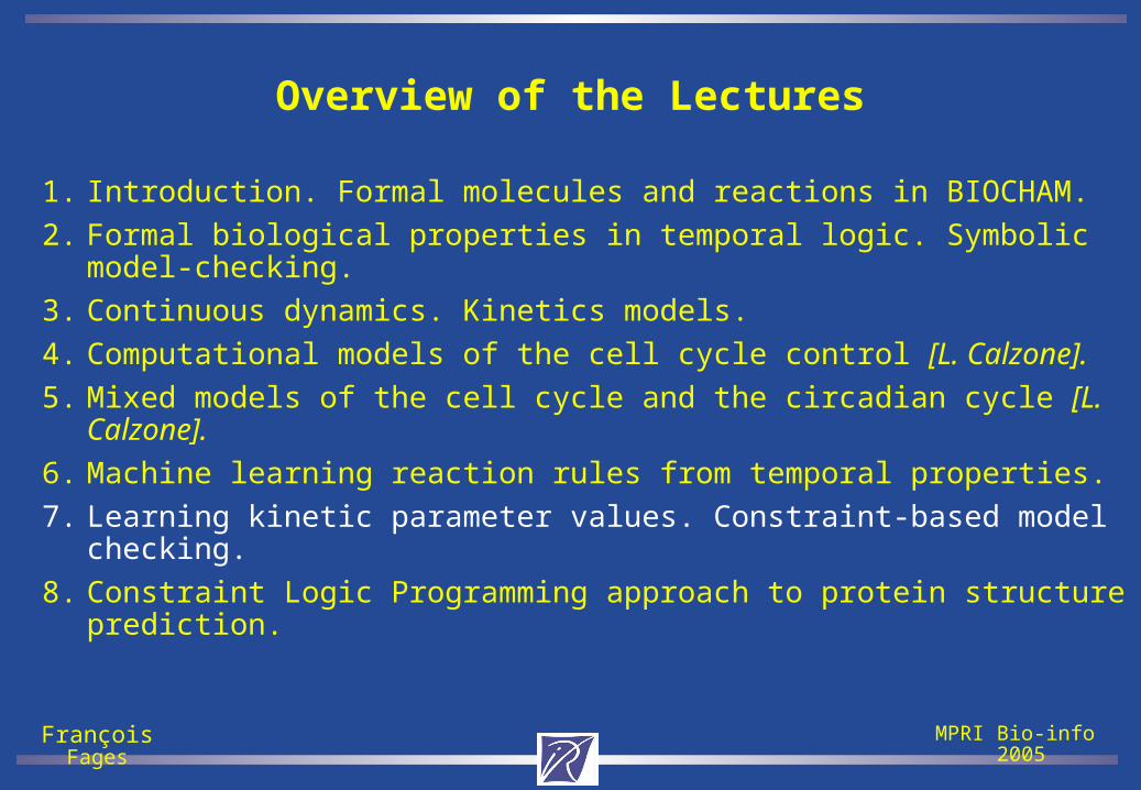
Overview of the Lectures
1. Introduction. Formal molecules and reactions in BIOCHAM.
2. Formal biological properties in temporal logic. Symbolic model-checking.
3. Continuous dynamics. Kinetics models.
4. Computational models of the cell cycle control [L. Calzone].
5. Mixed models of the cell cycle and the circadian cycle [L. Calzone].
6. Machine learning reaction rules from temporal properties.
7. Learning kinetic parameter values. Constraint-based model checking.
8. Constraint Logic Programming approach to protein structure prediction.
François Fages MPRI Bio-info 2005
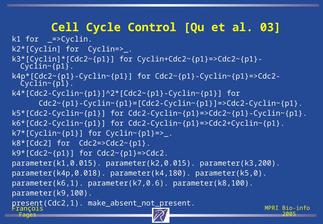
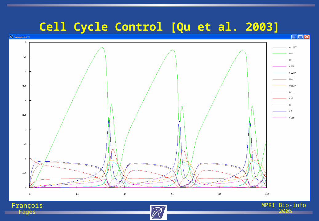
Cell Cycle Control [Qu et al. 03]k1 for _=>Cyclin.k2*[Cyclin] for Cyclin=>_.k3*[Cyclin]*[Cdc2~{p1}] for Cyclin+Cdc2~{p1}=>Cdc2~{p1}-Cyclin~{p1}.k4p*[Cdc2~{p1}-Cyclin~{p1}] for Cdc2~{p1}-Cyclin~{p1}=>Cdc2-Cyclin~{p1}.k4*[Cdc2-Cyclin~{p1}]^2*[Cdc2~{p1}-Cyclin~{p1}] for Cdc2~{p1}-Cyclin~{p1}=[Cdc2-Cyclin~{p1}]=>Cdc2-Cyclin~{p1}.k5*[Cdc2-Cyclin~{p1}] for Cdc2-Cyclin~{p1}=>Cdc2~{p1}-Cyclin~{p1}.k6*[Cdc2-Cyclin~{p1}] for Cdc2-Cyclin~{p1}=>Cdc2+Cyclin~{p1}.k7*[Cyclin~{p1}] for Cyclin~{p1}=>_.k8*[Cdc2] for Cdc2=>Cdc2~{p1}.k9*[Cdc2~{p1}] for Cdc2~{p1}=>Cdc2.parameter(k1,0.015). parameter(k2,0.015). parameter(k3,200).parameter(k4p,0.018). parameter(k4,180). parameter(k5,0).parameter(k6,1). parameter(k7,0.6). parameter(k8,100).parameter(k9,100).present(Cdc2,1). make_absent_not_present.
François Fages MPRI Bio-info 2005
Cell Cycle Control [Qu et al. 2003]
François Fages MPRI Bio-info 2005
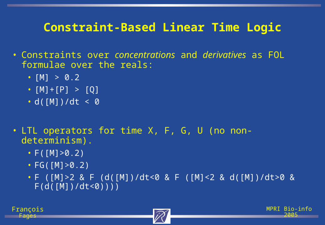
Constraint-Based Linear Time Logic
• Constraints over concentrations and derivatives as FOL formulae over the reals:
• [M] > 0.2
• [M]+[P] > [Q]
• d([M])/dt < 0
• LTL operators for time X, F, G, U (no non-determinism).• F([M]>0.2)
• FG([M]>0.2)
• F ([M]>2 & F (d([M])/dt<0 & F ([M]<2 & d([M])/dt>0 & F(d([M])/dt<0))))
François Fages MPRI Bio-info 2005
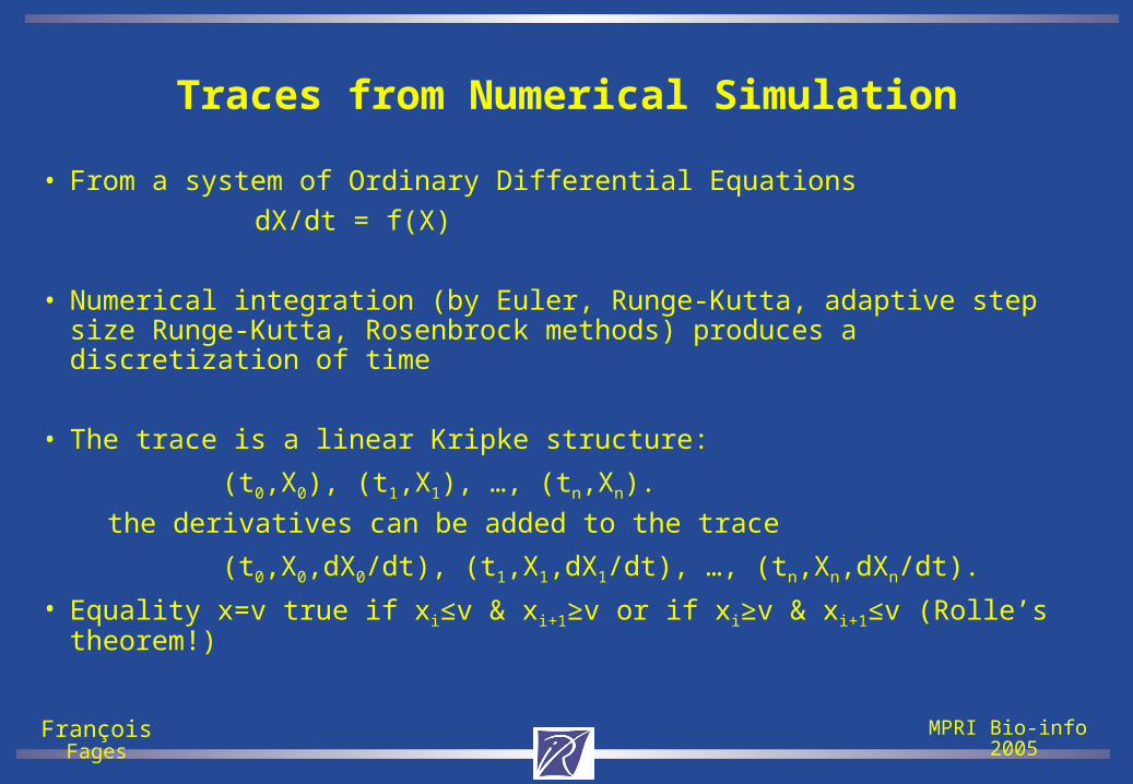
Traces from Numerical Simulation
• From a system of Ordinary Differential Equations
dX/dt = f(X)
• Numerical integration (by Euler, Runge-Kutta, adaptive step size Runge-Kutta, Rosenbrock methods) produces a discretization of time
• The trace is a linear Kripke structure:
(t0,X0), (t1,X1), …, (tn,Xn).
the derivatives can be added to the trace
(t0,X0,dX0/dt), (t1,X1,dX1/dt), …, (tn,Xn,dXn/dt).
• Equality x=v true if xi≤v & xi+1≥v or if xi≥v & xi+1≤v (Rolle’s theorem!)
François Fages MPRI Bio-info 2005
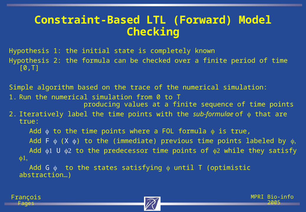
Constraint-Based LTL (Forward) Model Checking
Hypothesis 1: the initial state is completely known
Hypothesis 2: the formula can be checked over a finite period of time [0,T]
Simple algorithm based on the trace of the numerical simulation:
1. Run the numerical simulation from 0 to T producing values at a finite sequence of time points
2. Iteratively label the time points with the sub-formulae of that are true:
Add to the time points where a FOL formula is true,
Add F (X ) to the (immediate) previous time points labeled by Add U to the predecessor time points of while they satisfy Add G to the states satisfying until T (optimistic abstraction…)
François Fages MPRI Bio-info 2005
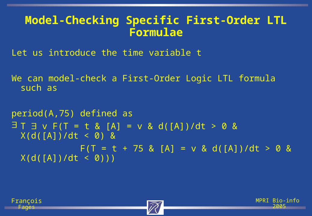
Model-Checking Specific First-Order LTL Formulae
Let us introduce the time variable t
We can model-check a First-Order Logic LTL formula such as
period(A,75) defined as T v F(T = t & [A] = v & d([A])/dt > 0 & X(d([A])/dt < 0) &
F(T = t + 75 & [A] = v & d([A])/dt > 0 & X(d([A])/dt < 0)))
François Fages MPRI Bio-info 2005
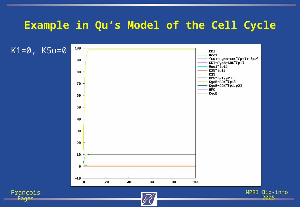
Example in Qu’s Model of the Cell Cycle
K1=0, K5u=0
François Fages MPRI Bio-info 2005
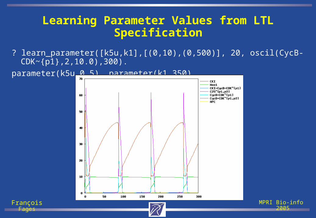
Learning Parameter Values from LTL Specification
? learn_parameter([k5u,k1],[(0,10),(0,500)], 20, oscil(CycB-CDK~{p1},2,10.0),300).
parameter(k5u,0.5). parameter(k1,350).
François Fages MPRI Bio-info 2005
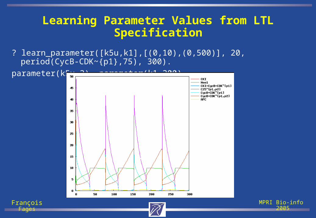
Learning Parameter Values from LTL Specification
? learn_parameter([k5u,k1],[(0,10),(0,500)], 20, period(CycB-CDK~{p1},75), 300).
parameter(k5u,2). parameter(k1,200).
François Fages MPRI Bio-info 2005
Backward Constraint-based Model Checking
Reason backward from the set of states satisfying a formula
to the set of initial states for which the formula is true.
Makes it possible to reason with a partially know initial state.
Approximate set of states with constraints: polyhedrons defined by linear constraints.
François Fages MPRI Bio-info 2005
Hybrid (Continuous-Discrete) Dynamics
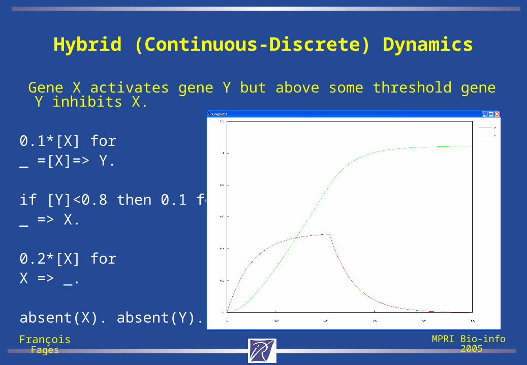
Gene X activates gene Y but above some threshold gene Y inhibits X.
0.1*[X] for _ =[X]=> Y.
if [Y]<0.8 then 0.1 for _ => X.
0.2*[X] for X => _.
absent(X). absent(Y).
François Fages MPRI Bio-info 2005
Translation to Constraint Logic Programs over Reals
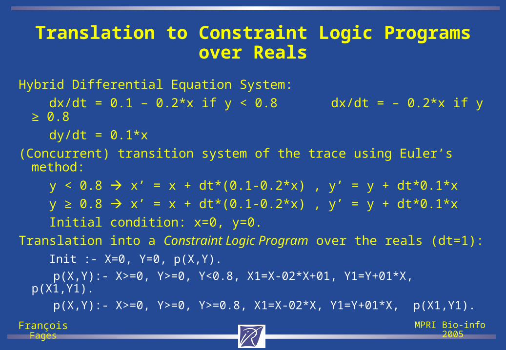
Hybrid Differential Equation System:
dx/dt = 0.1 – 0.2*x if y < 0.8 dx/dt = – 0.2*x if y ≥ 0.8
dy/dt = 0.1*x
(Concurrent) transition system of the trace using Euler’s method:
y < 0.8 x’ = x + dt*(0.1-0.2*x) , y’ = y + dt*0.1*x
y ≥ 0.8 x’ = x + dt*(0.1-0.2*x) , y’ = y + dt*0.1*x
Initial condition: x=0, y=0.
Translation into a Constraint Logic Program over the reals (dt=1):
Init :- X=0, Y=0, p(X,Y).
p(X,Y):- X>=0, Y>=0, Y<0.8, X1=X-02*X+01, Y1=Y+01*X, p(X1,Y1).
p(X,Y):- X>=0, Y>=0, Y>=0.8, X1=X-02*X, Y1=Y+01*X, p(X1,Y1).
François Fages MPRI Bio-info 2005
Constraint-based CTL Backward Model Checking
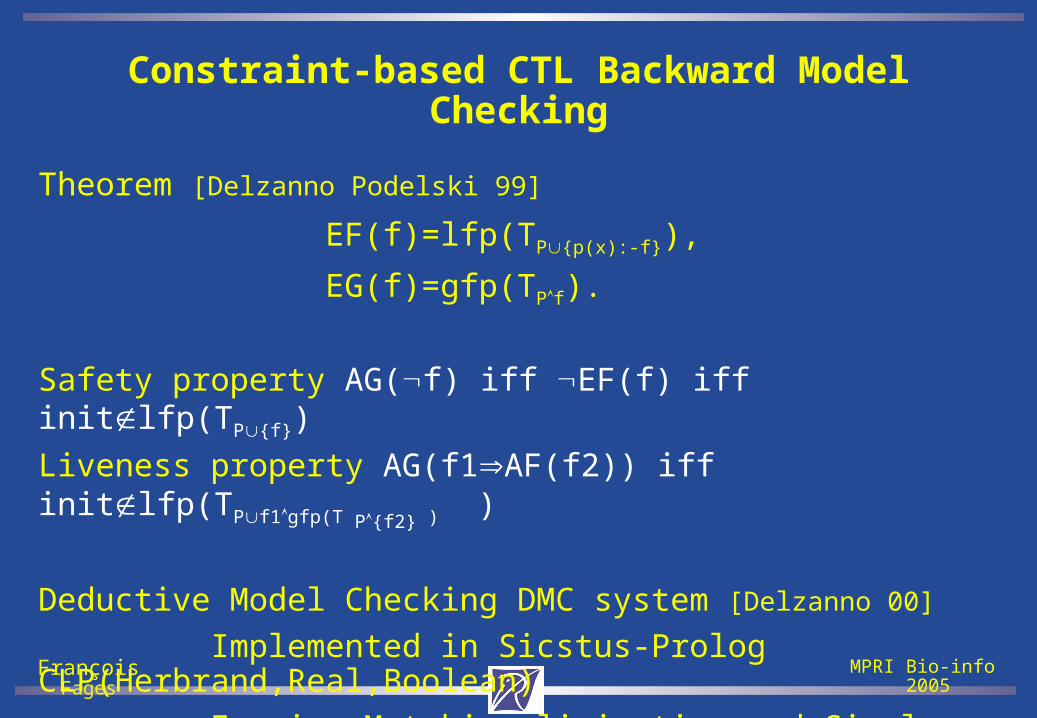
Theorem [Delzanno Podelski 99]
EF(f)=lfp(TP{p(x):-f}),
EG(f)=gfp(TPf).
Safety property AG(f) iff EF(f) iff initlfp(TP{f})
Liveness property AG(f1AF(f2)) iff initlfp(TPf1gfp(T P{f2} ) )
Deductive Model Checking DMC system [Delzanno 00]
Implemented in Sicstus-Prolog CLP(Herbrand,Real,Boolean)
Fourier-Motzkin elimination and Simplex algorithm.
François Fages MPRI Bio-info 2005
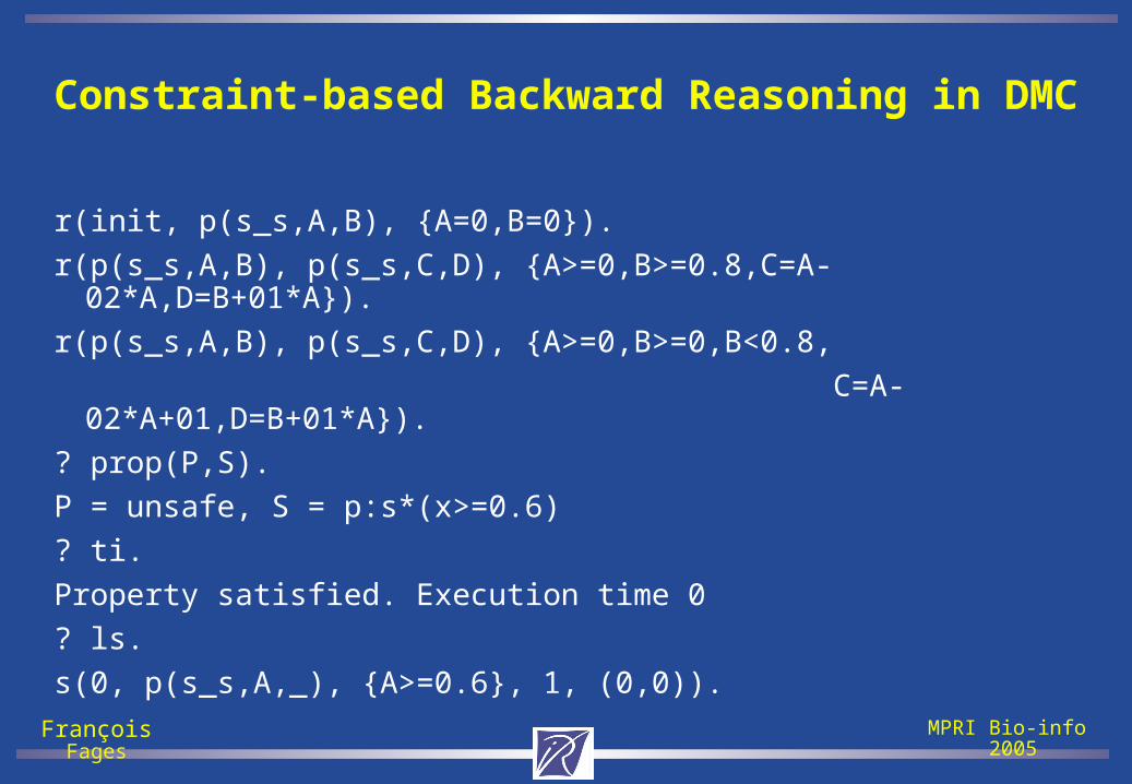
Constraint-based Backward Reasoning in DMC
r(init, p(s_s,A,B), {A=0,B=0}).
r(p(s_s,A,B), p(s_s,C,D), {A>=0,B>=0.8,C=A-02*A,D=B+01*A}).
r(p(s_s,A,B), p(s_s,C,D), {A>=0,B>=0,B<0.8,
C=A-02*A+01,D=B+01*A}).
? prop(P,S).
P = unsafe, S = p:s*(x>=0.6)
? ti.
Property satisfied. Execution time 0
? ls.
s(0, p(s_s,A,_), {A>=0.6}, 1, (0,0)).
François Fages MPRI Bio-info 2005
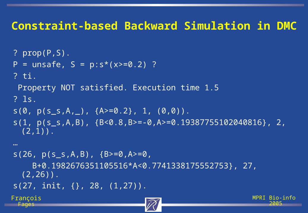
Constraint-based Backward Simulation in DMC
? prop(P,S).
P = unsafe, S = p:s*(x>=0.2) ?
? ti.
Property NOT satisfied. Execution time 1.5
? ls.
s(0, p(s_s,A,_), {A>=0.2}, 1, (0,0)).
s(1, p(s_s,A,B), {B<0.8,B>=-0,A>=0.19387755102040816}, 2, (2,1)).
…
s(26, p(s_s,A,B), {B>=0,A>=0,
B+0.1982676351105516*A<0.7741338175552753}, 27, (2,26)).
s(27, init, {}, 28, (1,27)).
Recommended