1
FORWARD-LOOKING ENERGY ELASTICITY PARAMETERS
FOR NESTED CES PRODUCTION FUNCTION
Oleg Lugovoy1
Vladimir Potashnikov2
Long abstract
Elasticities of substitution are the key parameters in CGE modeling.
However an estimation and validation of the parameters is not straightforward.
One of the ways is to use a historical data. Technological shifts between types of
fuels and capital and fuels, observed in the past, potentially could be used to
calibrate or econometrically estimate the elasticity coefficients. However,
historical trends do not describe all the possible investment options available now.
Moreover such estimates will be based on investment decisions made in particular
economic condition, policies, and available technological/investment options in the
time of decision. Application of the parameters for evaluation of future policy
options involves undesirable (and unavoidable) assumption that future
technological options are equal or similar to those in the past. A variety of new
technological options will be disregarded from the analysis.
A more natural way to model technological options is Bottom-Up
technological models. The reference energy system modes have an extensive
representation of energy sector, and take into account currently available and
expected technological options, but consider only part of an economy and lack
connectivity with other sectors, f.i. do not provide a demand respond. Therefore
their application is usually limited to the energy sector. There are several attempts
1 Environmental Defense Fund, USA, The Russian Presidential Academy of National Economy and Public
Administration, Moscow, Russia 2 The Russian Presidential Academy of National Economy and Public Administration, Moscow, Russia
2
to connect the top-down (CGE/AGE) and bottom-up models known as “soft” or
“hard link” (see f.i. Böhringer and Rutherford 2006, 2008). However both
methodologies require significant reduction of the models’ scale or some
compromise in connectivity between the models. The methodology proposed in the
paper might be considered as another way of hybrid modeling where bottom-up
model is used to calibrate parameters for a top-down model. It is expected, the
energy nest of a CGE model should provide results similar to the bottom-up model.
Methodology
The methodology included two stages. On the first stage we generate a
random sample of states of the world (SOW) and apply a multi-sector energy RU-
TIMES models for electric power, and iron and steel sectors to simulate a sample
of cost-efficient solutions for each of the randomly generated SOW. On the second
stage we apply econometrics to approximate the simulated sample of cost-efficient
solutions with a for-level nested CES production function. Comparing to historical
data, where only one (supposedly optimal) solution is observed for particular
economic conditions in the past, the randomly simulated sample represents a full
set of optimal solutions for a number of possible combination of unknown
variables (f.i. fuel prices). Therefore simulated data has an advantage over
historical in two ways. First, it takes into account currently available and expected
in the future technological options (in TIMES model). Second, simulated data
accommodates a huge variety of economic conditions which are not observable in
the real life, but theoretically possible.
Specification of numerical experiment
To generate a sample of optimal fuel mix structure under given economic
conditions, we apply a bottom-up model and solve it for various SOWs. Here are
the main specifications of the experiment:
3
1. Each economic sector is modeled separately (one bottom-up model for each
sector).
2. Time horizon is from 2010 to 2030.
3. Prices are randomly assigned for each commodity (coal, gas, oil) and each
SOW, and are constant for the all period of consideration.
4. Unlimited supply of each energy source under fixed price.
5. Final demand is growing with constant rate and equal for all SOW.
The only difference between SOWs is a set of energy prices (gas, oil, coal). We
performed 2000 model runs to generate a sample of the same size for CES
estimates.
Estimation of multi-level nested CES function
Estimation of CES function is not straightforward due to non-linearity.
There are several methods exist for one level functions. However it is even more
difficult to estimate multi-level, nested CES structure. In the paper we apply
Bayesian econometrics to estimate CES functions. The applied method is similar to
Tsurumi, Tsurumi (1976), but extended for multi-level cases. As a result, we
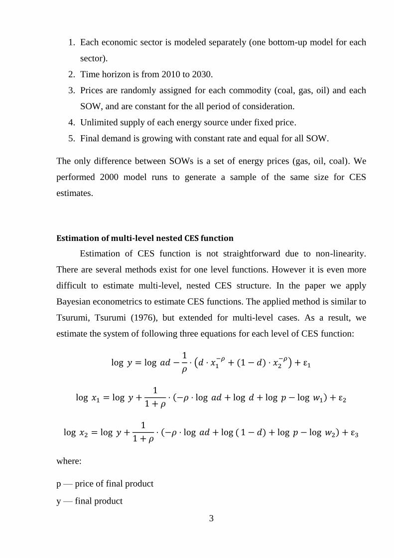
estimate the system of following three equations for each level of CES function:
where:
p — price of final product
y — final product
4
wi - price of production factor for CES production function
xi - production factor for CES production function
d — factor share parameter for CES production function
ad — productivity for CES production function
E — elasticity parameter for CES production function
ε — errors
ρ — elasticity parameter
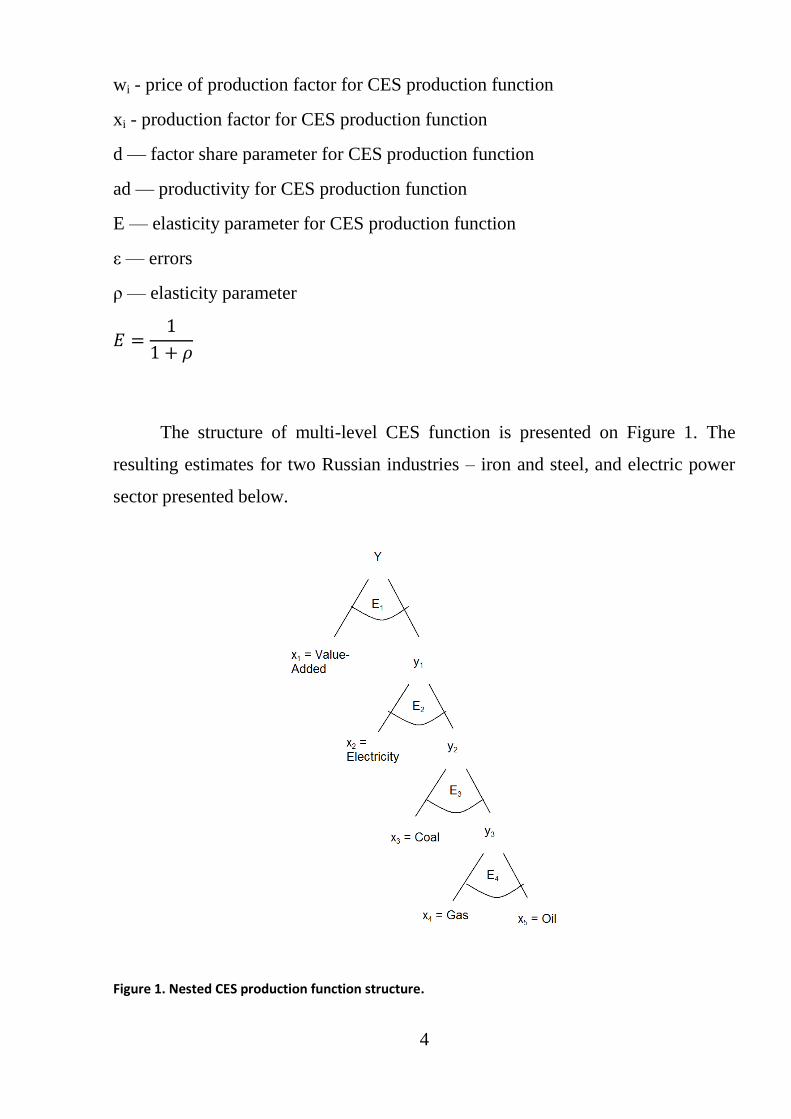
The structure of multi-level CES function is presented on Figure 1. The
resulting estimates for two Russian industries – iron and steel, and electric power
sector presented below.
Figure 1. Nested CES production function structure.
5
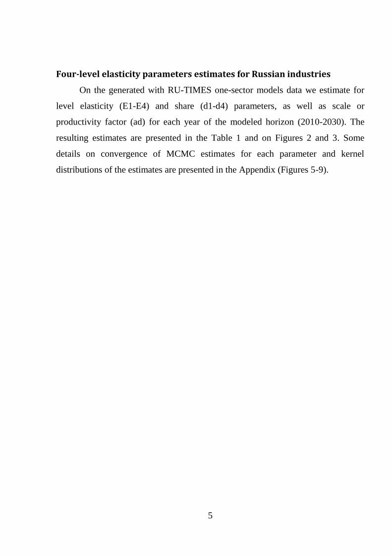
Four-level elasticity parameters estimates for Russian industries
On the generated with RU-TIMES one-sector models data we estimate for
level elasticity (E1-E4) and share (d1-d4) parameters, as well as scale or
productivity factor (ad) for each year of the modeled horizon (2010-2030). The
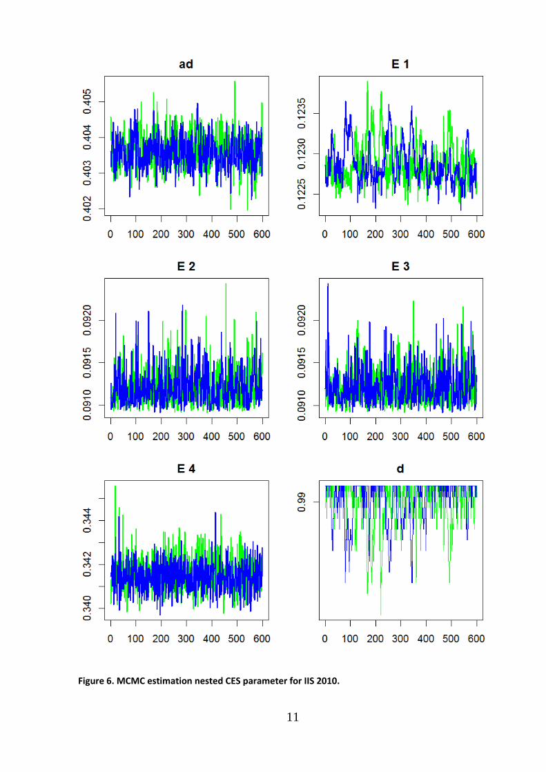
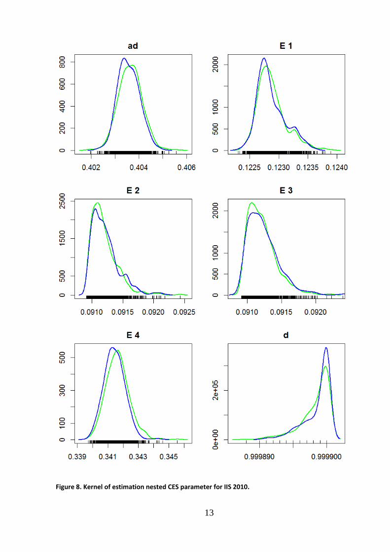
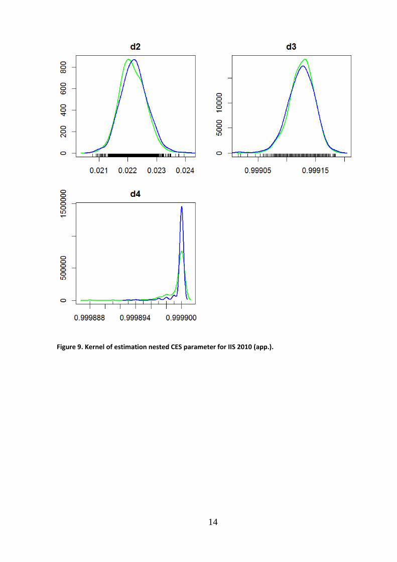
resulting estimates are presented in the Table 1 and on Figures 2 and 3. Some
details on convergence of MCMC estimates for each parameter and kernel
distributions of the estimates are presented in the Appendix (Figures 5-9).
6
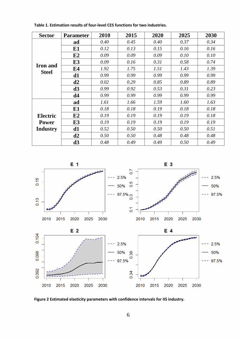
Table 1. Estimation results of four-level CES functions for two industries.
Sector Parameter 2010 2015 2020 2025 2030
Iron and
Steel
ad 0.40 0.45 0.40 0.37 0.34
E1 0.12 0.13 0.15 0.16 0.16
E2 0.09 0.09 0.09 0.10 0.10
E3 0.09 0.16 0.31 0.58 0.74
E4 1.92 1.75 1.51 1.43 1.39
d1 0.99 0.99 0.99 0.99 0.99
d2 0.02 0.29 0.85 0.89 0.89
d3 0.99 0.92 0.53 0.31 0.23
d4 0.99 0.99 0.99 0.99 0.99
Electric
Power
Industry
ad 1.61 1.66 1.59 1.60 1.63
E1 0.18 0.18 0.19 0.18 0.18
E2 0.19 0.19 0.19 0.19 0.18
E3 0.19 0.19 0.19 0.19 0.19
d1 0.52 0.50 0.50 0.50 0.51
d2 0.50 0.50 0.48 0.48 0.48
d3 0.48 0.49 0.49 0.50 0.49
Figure 2 Estimated elasticity parameters with confidence intervals for IIS industry.
7
As follows from the figure, the elasticity parameters have a tendency to
grow over time. This fact has an intuitive understanding that the possibility for
technological/fuel switch is higher when we have longer time.
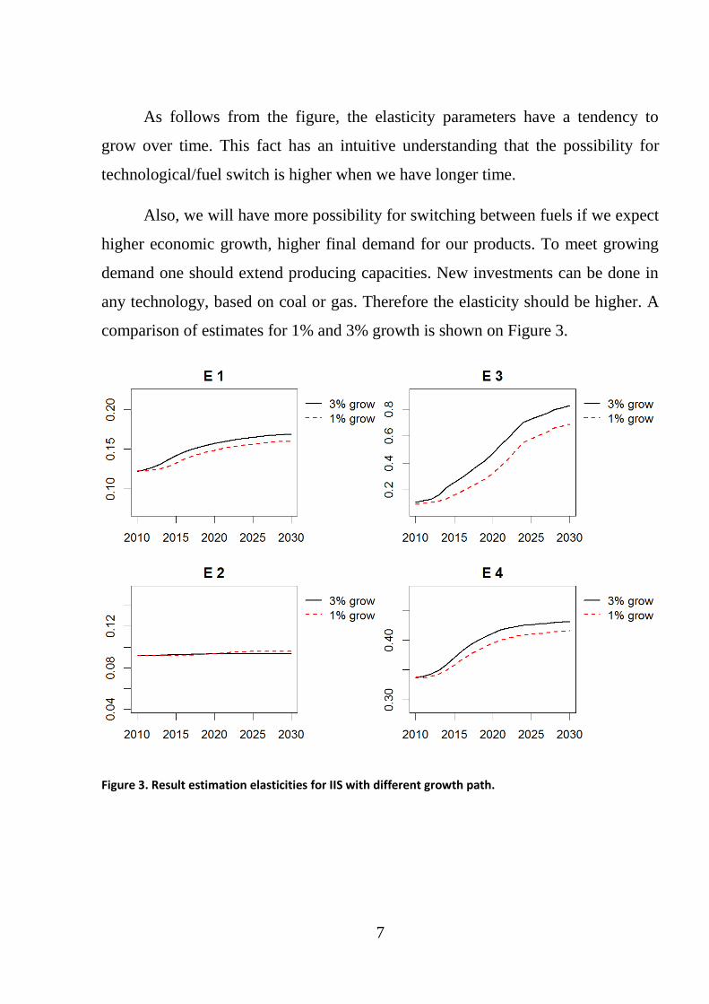
Also, we will have more possibility for switching between fuels if we expect
higher economic growth, higher final demand for our products. To meet growing
demand one should extend producing capacities. New investments can be done in
any technology, based on coal or gas. Therefore the elasticity should be higher. A
comparison of estimates for 1% and 3% growth is shown on Figure 3.
Figure 3. Result estimation elasticities for IIS with different growth path.
8
Some conclusions
The developed methodology applies bottom-up energy models to estimate
nested CES elasticity parameters for tom-down (CGE) models. The resulting
estimates have several advantages over historical elasticity parameters estimates.
First, they take into account all available now and in the future technological
options (based on bottom-up model specification). Second, they take into account
all possible set of economic variables, instead of only one observed in the past.
Therefore the methodology is much better in approximation of technological
switching.
There are several key observations should be mentioned regarding energy
elasticity parameters for the CGE modeling:
- Elasticity parameters depend on horizon of planning (experiment). Longer
horizon of planning usually lead to higher potential of switching between
fuels and technologies, i.e. elasticity parameters are higher.
- Assumption of higher economic growth should result in higher elasticity of
substitution. Currently existing capacities limit an opportunity for a
technological maneuver in the short and medium run periods. However
expansion of production assumes investments in new capacities.
- Technological shift and share parameters also depend on experiment horizon
and should be considered for adjustment in CGE experiments.
Estimates for transport, cement industry, and residential sectors are completed as
well and will be presented on the conference.
9
References
Christoph Bohringer. The synthesis of bottom-up and top-down in energy policy modeling.
Energy Economics, 20(3):233–248, 1998.
Christoph Bohringer and Thomas F. Rutherford. Combining bottom-up and top-down. Energy
Economics, 30(2):574–596, March 2008.
Thomas F. Rutherford and Christoph Böhringer. Combining top-down and bottom-up in energy
policy analysis: A decomposition approach. ZEW Discussion Papers 06-07, ZEW -Zentrum für
Europäische Wirtschaftsforschung / Center for European Economic Research, 2006.
Heinz Welsch Claudia Kemfert. Energy-capital-labor substitution and the economic effects of
co2 abatement: Evidence for germany. Journal of Policy Modeling, 22(6):641–660, November
2000
Edwin van der Werf. Production functions for climate policy modeling: An empirical analysis.
Energy Economics, 30(6):2964–2979, November 2008.
Arne Henningsen and Géraldine Henningsen. On estimation of the ces production function—
revisited. Economics Letters, 115(1):67–69, 2012.
Henningsen, A. and Henningsen, G. Econometric Estimation of the Constant Elasticity of
Substitution Function in R: Package micEconCES, FOI Working Paper 2011 / 9
Rins Harkema and Sybrand Schim van der Loeff. On bayesian and non-bayesian estimation of a
two-level ces production function for the dutch manufacturing sector. Journal of Econometrics,
5:155–165, 1977.
Yoshi Tsurumi Hiroki Tsurumi. A bayesian estimation of macro and micro ces production
functions. Journal of Econometrics, 4: 1–25, 1976.
V. K. Chetty and U. Sankar. Bayesian estimation of the ces production function. The Review of
Economic Studies, 36:289–294, 1969.
B. S. Minhas K. J. Arrow, H. B. Chenery and R. M. Solow. Capital-labor substitution and
economic efficiency. The Review of Economics and Statistics, 43(3):225–250, 1961.
J. Kmenta. On estimation of the ces production function. International Economic Review,
8(2):180–189, 1967.
Jerry G Thursby and C A Knox Lovell. An investigation of the kmenta approximation to the ces
function. International Economic Review, 19(2):363–77, June 1978.
10
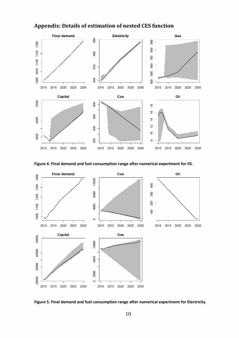
Appendix: Details of estimation of nested CES function
Figure 4. Final demand and fuel consumption range after numerical experiment for IIS.
Figure 5. Final demand and fuel consumption range after numerical experiment for Electricity.
11
Figure 6. MCMC estimation nested CES parameter for IIS 2010.
12
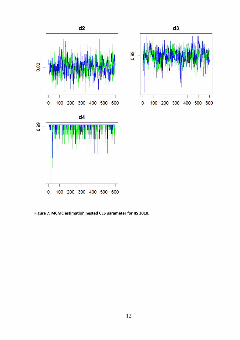
Figure 7. MCMC estimation nested CES parameter for IIS 2010.
13
Figure 8. Kernel of estimation nested CES parameter for IIS 2010.
14
Figure 9. Kernel of estimation nested CES parameter for IIS 2010 (app.).
Recommended


![Looking back and looking forward[1]](https://img.dokumen.tips/doc/110x75/5559ad0dd8b42aa4288b511b/looking-back-and-looking-forward1.jpg)


