Download pdf - EXACT SHAPE FUNCTIONS AND TANGENT STIFFNESS …webserver2.tecgraf.puc-rio.br/~lfm/papers/BurgosCilamce2013.pdf · Some examples of stability analysis of this finite element formulation

P

EXAFOR

Rodrigo

rburgos

Rio de J

Rua São

Luiz Fe

lfm@te

Pontific

Rua Ma

Abstracequationconsidethere isexplicitlfunctionelastic fand somthe procriteria

Keywor

Proceedings o

ACT SHATHE BU

o Bird Bur

@ig.com.br

Janeiro Stat

o Francisco

ernando C.

cgraf.puc-ri

cal Catholic

arquês de Sã

ct. This papns. These d

ering a two-s a need foly and discuns, stiffnessfoundation.

me examplesoblem of ch

are establis

rds: Bucklin

f the XXXIV Z.J.G.N D

APE FUNCUCKLING

rgos

r

te Universit

Xavier, 524

. R. Martha

io.br

University

ão Vicente,

per is baseddifferential -parameter for an implusses the d

s matrices a Taylor sers are studiehoosing beshed.

ng, Timoshe

Iberian LatinDel Prado (Ed

CTIONSG OF BEA

DEF

y (UERJ)

4, 20550-90

a

of Rio de J

225, 22453

d on exact sequations aelastic founlementation

different posand equivaries are useed in order tetween exac

enko beam th

-American Coditor), ABMEC

AND TAAM-COLFORMAT

00, Rio de J

Janeiro (PU

3-900, Rio d

solutions ofare obtainendation. Altn-oriented wssibilities ofalent load fed to obtainto compare ct and app

heory, Diffe

ongress on CoC, Pirenópolis

ANGENT UMNS C

TION

Janeiro, RJ,

C-Rio)

de Janeiro, R

f axially loaed for the Tthough theswork whichf approximaforces is prn different tyresults. Thi

proximate m

erential equ

omputational Ms, GO, Brazil,

STIFFNEONSIDE

Brazil

RJ, Brazil

aded beam-Timoshenkose solutionsh presents ation. The dresented fortypes of appis paper is amethods an

uations

CILAMMethods in EnNovember 10

ESS MATRING SH

-column diffo beam thes are widely

the problederivation or the case proximate salso concernnd some nu

MCE 2013 ngineering 0-13, 2013

TRIX HEAR

fferential ory also y known, em more of shape with no

solutions ned with umerical

Exact shape functions and tangent stiffness matrix

CILAMCE 2013 Proceedings of the XXXIV Iberian Latin-American Congress on Computational Methods in Engineering Z.J.G.N Del Prado (Editor), ABMEC, Pirenópolis, GO, Brazil, November 10-13, 2013

1 INTRODUCTION

Current structural engineering design codes proclaim the consideration of geometric nonlinear effects in structural analysis. In frame analysis, these effects are usually considered through a stability or second-order analysis. In addition, modern frame analysis takes into account shear deformation of structural elements (Timoshenko beam theory).

Second-order stability analysis of slender columns is a well know problem with available analytical solution and second-order stability analysis of framed structures with slender beam-columns have been studied by numerous researchers because of their importance in structural engineering. A frame structure stability analysis may be performed in many different ways, ranging from simple verifications based on first-order linear analysis to sophisticated higher-order nonlinear numerical analysis. The objective of this type of analysis is the evaluation of critical loads that would cause structural buckling, while still considering small deformations. Although there are analytical solutions for simple frame second-order stability analysis, in general a numerical solution is employed and many existing computer programs are able to perform this type of analysis. However, since second-order stability analysis is based on a set of simplifications, numerical solutions depend on discretization of structural members. This means that the analyst must have some experience on this type of analysis in order to adequately define the number of segments that should be used in the discretization of a structural member. To decrease the influence on arbitrary member discretization, higher-order stability analysis is required.

Nevertheless, second or higher order stability analysis of frame structures considering shear deformation has very few available solutions in the literature (Onu, 2000 and 2008, Areiza-Hurtado et al. 2005). Generally, the shear effect is immaterial for slender beams. However, in the case of the skeletal structures, if the length-to-depth ratio of foundation beams is relatively small and these beams are subjected to discrete column loads, the shear effect becomes important and must be taken into account. This problem is still an open issue that requires further investigation and is the focus of this work.

In addition to the problem of stability analysis, a complete formulation of the static behavior of beam-column members should consider transversal elastic foundations, which is an important effect in foundation beams. In the literature there are few papers that formulate the combined effect of transversal loading, axial compression (stability analysis), shear deformation (Timoshenko beam theory), and transversal elastic foundations.

Most of the works considers pair-wise combinations of these effects. For example, Nukulchai et al. (1981) formulated exact solutions for beam finite elements taking into account Timoshenko’s shear deformation. Zhaohua & Cook (1983) presented finite beam element solutions considering a two-parameter (displacement and rotation) elastic foundation, but with no shear deformation. Ting & Mockry (1984) defined finite element solutions for beams considering only displacement elastic foundations and no shear deformation. Eisenberger & Yankelevsky (1984) also formulated exact solutions for beam on displacement elastic foundation with no shear deformation. Chiwanga & Valsangkar (1988) presented a stiffness matrix and equivalent nodal forces for beam elements considering a two-parameter elastic foundation with no shear deformation. Shrima & Giger (1992) formulated Timoshenko’s beam finite elements resting on two-parameter elastic foundation. These authors created an auxiliary function, which is used in this work, to solve analytically the differential equations of this problem. Bazant & Cedolin (1991) presented the solutions for

R. B. Burgos, L. F. C. R. Martha

CILAMCE 2013 Proceedings of the XXXIV Iberian Latin-American Congress on Computational Methods in Engineering

Z.J.G.N Del Prado (Editor), ABMEC, Pirenópolis, GO, Brazil, November 10-13, 2013

stability analysis of columns considering shear deformations. Ready (1997) and Ready et al. (1997) extended the finite element formulation of beams with shear deformation to consider also cross section warping, without considering elastic foundation or axial load effects. Onu (2000) considered Timoshenko’s shear effect in a beam finite element on two-parameter elastic foundation. Morfidis & Avramidis (2002) formulated a generalized beam element on a two-parameter elastic foundation with semi-rigid connections and rigid offsets. Areiza-Hurtado et al. (2005) presented a solution for second-order stiffness matrix and loading vector of a beam-column with semirigid connections on a single-parameter elastic foundation. Morfidis (2007) formulated exact matrices for Timoshenko’s beams on three-parameter elastic foundation, with no second-order axial load effect. Onu (2008) was the first author to consider the combined effect of second-order stability due to axial load, transversal loading, shear deformation and two-parameter elastic foundation. However, that work presented a synthetic formulation that is difficult to reproduce and does not present formulations of analytical shape functions.

Analytical solutions for generalized beam finite elements are available. However, it was not found in the literature a work that didactically formulates the problem in an unified form, considering transversal loading, Timoshenko’s shear deformation, axially loaded stability high-order effects, and two-parameter (displacement and rotation) elastic foundation. This paper presents a unified analytical formulation of these combined effects on a beam-column. The main objective is to present analytical and higher-order solutions of shape functions, tangent stiffness matrix and equivalent load forces including the effects of shear deformation in an axially loaded prismatic beam-column member. These finite element solutions do not consider elastic foundations, which is left for a future work. It should be pointed out that, although higher-order stability effects are considered (large displacements), the assumption of a small deformation is maintained.

The paper is organized in the following manner: the next section introduces the differential equations that govern the problem of beam-columns resting on a two-parameter elastic foundation, subjected to transversal loading, considering Timoshenko’s shear deformation and axial-loading effects, with small deformations. Section 3 presents analytical and higher-order solutions of shape functions, tangent stiffness matrix and equivalent load forces including the effects of shear deformation in an axially loaded prismatic beam-column member, with no elastic foundation. Some examples of stability analysis of this finite element formulation are presented in Section 4. A discussion on the high-order terms that should be considered in stability analysis of frames is presented. Finally, Section 5 summarizes the conclusions of this work and points to future developments.

2 DIFFERENTIAL EQUATIONS

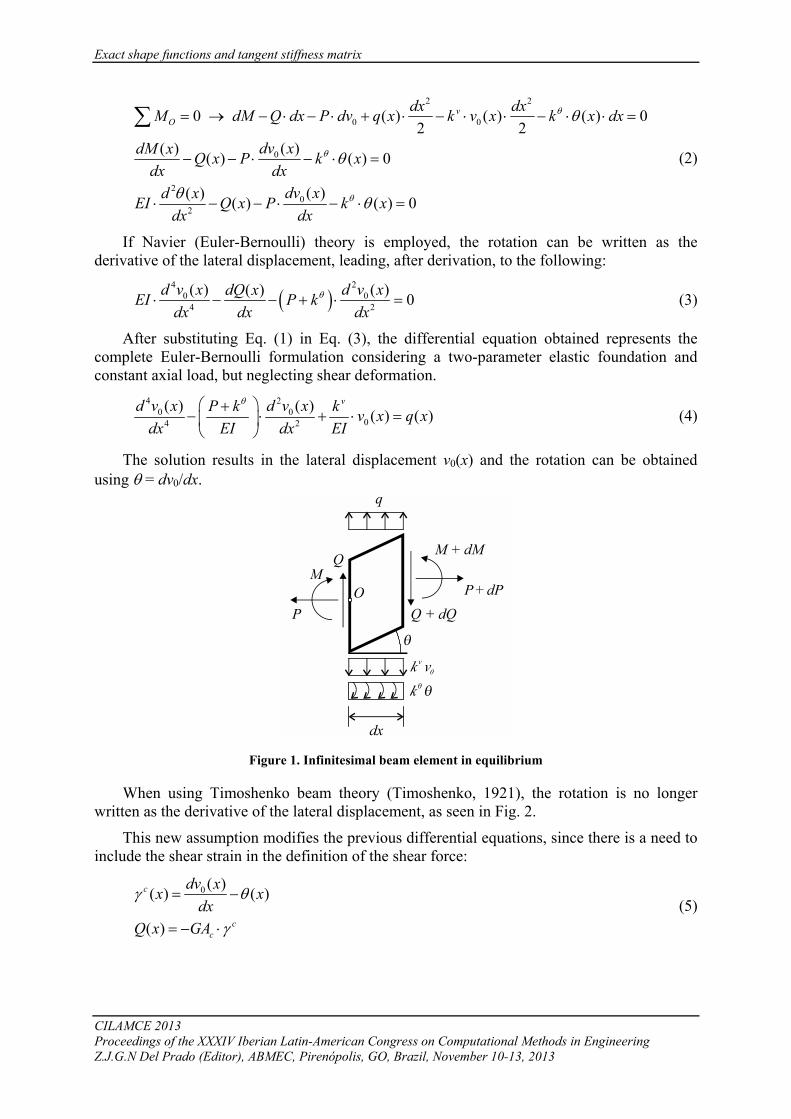
Figure 1 shows the deformed configuration of an infinitesimal beam element on a two-parameter elastic foundation subjected to transversal (q) and axial (P) loads.

The elastic foundation reactions are given by a force per unit length proportional to the lateral displacement and a moment per unit length proportional to the cross-section rotation. Considering all forces involved, equilibrium imposition leads to the following equations:

0 00 ( ) ( ) 0 ( ) ( )v vy

dQF dQ q x dx k v x dx q x k v xdx

= → − + ⋅ − ⋅ ⋅ = → = − ⋅∑ (1)



2 2

0 0

0

20

2

0 ( ) ( ) ( ) 02 2

( )( ) ( ) ( ) 0

( )( ) ( ) ( ) 0

vO

dx dxM dM Q dx P dv q x k v x k x dx

dv xdM x Q x P k xdx dx

dv xd xEI Q x P k xdx dx

θ

θ

θ

θ

θ

θ θ

= → − ⋅ − ⋅ + ⋅ − ⋅ ⋅ − ⋅ ⋅ =

− − ⋅ − ⋅ =

⋅ − − ⋅ − ⋅ =

∑

(2)

If Navier (Euler-Bernoulli) theory is employed, the rotation can be written as the derivative of the lateral displacement, leading, after derivation, to the following:

( )4 2

0 04 2

( ) ( )( ) 0d v x d v xdQ xEI P kdx dx dx

θ⋅ − − + ⋅ = (3)

After substituting Eq. (1) in Eq. (3), the differential equation obtained represents the complete Euler-Bernoulli formulation considering a two-parameter elastic foundation and constant axial load, but neglecting shear deformation.

4 20 0

04 2

( ) ( ) ( ) ( )vd v x d v xP k k v x q x

dx EI dx EI

θ⎛ ⎞+− ⋅ + ⋅ =⎜ ⎟

⎝ ⎠ (4)

The solution results in the lateral displacement v0(x) and the rotation can be obtained using θ = dv0/dx.

Figure 1. Infinitesimal beam element in equilibrium

When using Timoshenko beam theory (Timoshenko, 1921), the rotation is no longer written as the derivative of the lateral displacement, as seen in Fig. 2.

This new assumption modifies the previous differential equations, since there is a need to include the shear strain in the definition of the shear force:

0 ( )( ) ( )

( )

c

cc

dv xx xdx

Q x GA

γ θ

γ

= −

= − ⋅ (5)




Figure 2. Cross-section rotation and shear strain in Timoshenko beam theory

The substitution of Eq. (5) in Eqs. (1) and (2) leads to: 2

00 02

( )( )( ) ( ) ( ) ( )v vc

d v xdQ d xq x k v x GA k v x q xdx dx dx

θ⎛ ⎞= − ⋅ → ⋅ − + ⋅ =⎜ ⎟

⎝ ⎠ (6)

20 0

2

( ) ( )( ) ( ) ( ) 0cdv x dv xd xEI GA x P k x

dx dx dxθθ θ θ⎛ ⎞⋅ + ⋅ − − ⋅ − ⋅ =⎜ ⎟

⎝ ⎠ (7)

Equations (6) and (7) are coupled due to the term kvv0(x) in Eq. (6). This fact makes it impossible to solve for θ(x) separately. It’s possible to isolate v0(x), but with loss of shear information, which takes the problem back to the Euler-Bernoulli approach and the need to take shear deformation into account later. One possible strategy to uncouple Eqs. (6) and (7) is to rewrite the latter, collecting alike terms in θ and v0:

( )( )( ) ( )

20 0

2

20

2

( ) ( )( ) ( ) 0

( ) ( )( )

c c

c

c c

dv x dv xd xEI GA P GA k xdx dx dx

GA kdv x EI d xxdx GA P GA P dx

θ

θ

θ θ

θθ

⋅ + ⋅ − ⋅ − + ⋅ =

+= −

− −

(8)

An auxiliary function f(x) is then created with the following property (Shirima & Giger, 1992):

( )( ) ( )

2

0 2

( )( )

( )( ) ( )c

c c

df xxdxGA k EI d f xv x f xGA P GA P dx

θ

θ =

+= −

− −

(9)

It can be easily noticed that when shear deformation is neglected, i. e., GAc = ∞, the auxiliary function f(x) coincides with the displacement function v0(x) and the cross-section rotation is the displacement gradient. In other words, the solution simplifies to the Euler-Bernoulli case. It’s also evident that without an elastic foundation the term kvv0(x) vanishes and there is no need to use the auxiliary function f(x). This will be the case in this paper.

Substituting the expressions in Eq. (9) for f(x) in Eq. (6): 4 2

4 2

( ) ( ) ( )1 ( ) 1v v

c c c

d f x k P k d f x k k P q xf xdx GA EI dx EI GA GA EI

θ θ⎛ ⎞ ⎛ ⎞ ⎛ ⎞+− + ⋅ + ⋅ + ⋅ = −⎜ ⎟ ⎜ ⎟ ⎜ ⎟

⎝ ⎠ ⎝ ⎠ ⎝ ⎠ (10)



Equation (10) is the differential equation for the complete problem, i. e., considering shear deformation (Timoshenko beam), two-parameter elastic foundation (translational and rotational) and axial load (taken as a constant within the beam). Its solution is the function f(x). The cross-sectional rotation θ(x) and the lateral displacement v0(x) are then obtained from f(x) through Eq. (9).

The characteristic polynomial of the differential equation in Eq. (10) is given by:

4 2 1 0v v

c c

k P k k kGA EI EI GA

θ θ

λ λ⎛ ⎞ ⎛ ⎞+

− + + + =⎜ ⎟ ⎜ ⎟⎝ ⎠ ⎝ ⎠

(11)

Equation (11) can be conveniently written in the following form (Simmons, 1972):

4 2 2 12 0, 1 ,2

v v

c c

k k k P kEI GA GA EI

θ θ

λ β λ α α β⎛ ⎞ ⎛ ⎞+

− + = = + = +⎜ ⎟ ⎜ ⎟⎝ ⎠ ⎝ ⎠

(12)

The roots of the characteristic polynomial are given by:

( )

2 21...4

22 2 1 1

4

v v

c c


θ θ

λ β β α

β α

= ± ± −

⎡ ⎤⎛ ⎞ ⎛ ⎞+⎢ ⎥− = + − +⎜ ⎟ ⎜ ⎟⎢ ⎥⎝ ⎠ ⎝ ⎠⎣ ⎦

(13)

An initial analysis of these roots leads to the following conclusions:

1) In case (β2-α2) > 0, the first square root is a real number smaller than β, which guarantees four different real roots for λ. Some special cases can be suggested, neglecting one or more of the parameters involved, but in the complete model it’s difficult to predict when this combination can occur.

2) The only possibility of complex roots for λ appears when (β

2-α2) < 0. In the case of P being negative (compression), the squared term becomes smaller, increasing the possibility of complex roots. According to Zhaohua and Cook (1983), in general (kθ)2 ≤ 4EIkv, therefore it is reasonable to assume that the roots will be complex. However, a deeper investigation is necessary.

In the case of complex roots in the form a biλ = ± ± (2 pairs of complex conjugates), the following may be written:

( )2 2 2 2 22a b abi iλ β α β= − ± = ± − (14)

Solving for a and b: 2 2 2 2 2 2, 2

,2 2

a b ab a b

a b

β α β α

α β α β

− = = − → + =

+ −= =

(15)

The homogeneous solution for the differential equation assuming four independent roots 1 2 3 4, , ,λ λ λ λ is given by:

31 2 4( ) xx x xf x Ae Be Ce Deλλ λ λ= + + + (16)




Since the problem is modeled using a fourth-order differential equation, the homogeneous solution must be composed of four linearly independent functions. Therefore, if some multiplicity of roots is verified, i. e., if λi = λj for i ≠ j, some additional polynomial functions are used (this is only possible for real roots, since complex roots always appear in complex conjugate pairs). For example, if λ1 = λ2, solution is given by

31 4( ) ( ) xx xf x e A Bx Ce Deλλ λ= + + + .

It is interesting to notice that if there is no elastic foundation (kv = kθ = 0) and no axial load (P = 0), all four roots of the characteristic polynomial are null, i. e.,

1 2 3 4 0λ λ λ λ λ= = = = = , leading to:

2 3( ) ( )xf x e A Bx Cx Dxλ= + + + (17)

Since λ = 0, the solution is a cubic polynomial, which is the homogeneous solution for the differential equation of the classical Timoshenko beam.

In the general case of four independent complex roots, the homogeneous solution using 1...4 a biλ = ± ± is given by:

[ ] [ ][ ] [ ]

31 2 4

1 2 3 4

( )( ) cos( ) sen( ) cos( ) sen( )

( ) cosh( ) cos( ) sen( ) senh( ) cos( ) sen( )

xx x x

ax ax

f x Ae Be Ce Def x e A bx B bx e C bx D bx

f x ax c bx c bx ax c bx c bx

λλ λ λ

−

= + + +

= + + +

= ⋅ ⋅ + ⋅ + ⋅ ⋅ + ⋅

(18)

Equation (18) is the general solution for f(x) in Eq. (16), with a and b given by Eq. (15), which depend on α and β, given by Eq. (12).

2.1 Special cases

Some special combinations of the parameters involved can lead to particular cases. Some of those are presented below:

1) α = β

In this case, root multiplicity occurs and no complex roots will appear. The solution is given by:

1( ) ( ) ( ), ,2

vax ax

c

k P kf x e A Bx e C Dx aGA EI

θ

β β− ⎛ ⎞+= + + + = = +⎜ ⎟

⎝ ⎠ (19)

For this case the following must be verified: 2

4 1v v

c c


θ θ⎛ ⎞ ⎛ ⎞++ = +⎜ ⎟ ⎜ ⎟

⎝ ⎠ ⎝ ⎠ (20)

A deeper investigation is necessary to predict if this case is physically possible.

2) GAc = ∞ (Euler-Bernoulli beam)

Considering Eq. (10) and GAc = ∞, it’s obvious that it simplifies into Eq. (3), which represents the Euler-Bernoulli complete model. This means that the lateral displacement v0(x) is equal to the general solution f(x):



[ ] [ ]0 1 2 3 4( ) cosh( ) cos( ) sen( ) senh( ) cos( ) sen( )

2 2 2

v

v x ax c bx c bx ax c bx c bx

k N ka bEI EI

θα β α β α β

= ⋅ ⋅ + ⋅ + ⋅ ⋅ + ⋅

+ − += = = =

(21)

2a) N = 0, GAc = ∞ (Euler-Bernoulli beam without axial load)

The expression for v0(x) is also given by Eq. (21) with:

2 2 2

vk ka bEI EI

θα β α β α β+ −= = = = (22)

2b) kθ = 0, N = 0, GAc = ∞ (classical case of one-parameter elastic foundation)

The expression for v0(x) is also given by Eq. (21) with:

4

2 4

vka bEI

α= = = (23)

2c) kθ = kv = 0, N = 0, GAc = ∞ (axially loaded beam without elastic foundation)

In this case there is root multiplicity and the expression v0(x) for must take this into account with the inclusion of a polynomial solution.

( )

4 22 20 0

4 2

2 2 21,2 3 4

0

( ) ( ) 0,

0 0, ,

( ) x x

d v x d v x Pdx dx EI

v x Ae Be Cx Dμ μ

μ μ

λ λ μ λ λ μ λ μ−

− ⋅ = =

− = → = = = −

= + + +

(24)

In the case of a positive P (tension), μ is a real number and the expression for v0(x) can be written in terms of hyperbolic functions. In the case of a negative P (compression), μ is complex and the expression for v0(x) can be written in terms of trigonometric functions.

For a compressive axial load (P < 0) the following applies:

0 1 2 3 4( ) sen( ) cos( ) , Pv x c x c x c x cEI

μ μ μ −= ⋅ + ⋅ + ⋅ + = (25)

For a tensile axial load (P < 0) the following applies:

0 1 2 3 4( ) senh( ) cosh( ) , Pv x c x c x c x cEI

μ μ μ= ⋅ + ⋅ + ⋅ + = (26)

When working directly with the exponential solution, there is no need to make that separation of compression and tension cases. The only issue is that the implementation must consider the possibility of dealing with complex variables.

3) kθ = kv = 0 (Timoshenko beam without elastic foundation)

In the case of no elastic foundation it is possible to uncouple the equations and find a solution in terms of θ(x). This will be the case of study of this paper. Equation (6) becomes:

20

2

( )( ) ( )

c

d v xd x q xdx dx GAθ

− = (27)




Substituting Eq. (27) in the derivative of Eq. (7), with kθ = 0: 3

3

( ) ( ) ( )1

c

d x P d x q xdx dxPEI

GA

θ θ− ⋅ =

⎛ ⎞+⎜ ⎟

⎝ ⎠

(28)

After determining θ(x) from Eq. (28), the lateral displacement v0(x) can be obtained using Eq. (8) with kθ = 0:

20

2

( ) ( )( )c

c c

dv x GA EI d xxdx GA P GA P dx

θθ= −− −

(29)

3 EXACT FINITE ELEMENT IMPLEMENTATION

Considering Timoshenko beam theory and the differential equations given in Eqs. (28) and (29), the exact shape functions for an axially loaded beam can be derived. It is useful to remind that in the case of no elastic foundation, the equations can be uncoupled and the solution is given in terms of the rotation.

The homogeneous solution of Eq. (28) in terms of the cross-section rotation is given by:

2( ) ,1

x x

c

Px Ae Be CPEI

GA

μ μθ μ−= + + =⎛ ⎞

+⎜ ⎟⎝ ⎠

(30)

Substituting eq. (30) in eq. (29):

( ) ( )2 20

0

( )

( )

x x x xc

c c

x x c

c

dv x GA EIAe Be C A e B edx GA P GA P

dv x GAAe Be Cdx GA P

μ μ μ μ

μ μ

μ μ− −

−

= + + − +− −

= + +−

(31)

Integrating Eq. (31) respect to x:

0 ( ) x x c

c

GAA Bv x e e Cx DGA P

μ μ

μ μ−= − + +

− (32)

It’s interesting to notice that, as in classic Timoshenko beam theory (with no elastic foundation or axial load), only the first degree term of the polynomial solution is modified by the consideration of shear deformation. It’s also easy to notice that in the case of GAc = ∞, θ(x) becomes the derivative of v0(x) and the expression for v0(x) turns into Eq. (24) (axially loaded Euler-Bernoulli beam).

Using Eqs. (30) and (32), the expressions for v0(x) and θ(x) can be written in terms of four independent constants:

( )

0 1 2 3 4

1 2 32 2

22 2 2

( )

( )

1 1, ,1 2 1

x x

x x

c

c c c

v x c e c e c x c

x c e c e c

GA L EI PGA P L GA L EI P GA

μ μ

μ μ

η

θ μ μ

μη μμ

−

−

= ⋅ + ⋅ + ⋅ ⋅ +

= ⋅ ⋅ − ⋅ ⋅ +

− Ω= = Ω = =

− − Ω +

(33)



In matrix form, these conditions are given as:

[ ] { }

{ } { }

[ ]

0

T1 2 3 4

( )( )

11 0

x x

x x

v xX C

x

C c c c c

e e xX

e e

μ μ

μ μ

θ

ημ μ

−

−

⎧ ⎫= ⋅⎨ ⎬

⎩ ⎭

=

⎡ ⎤⋅= ⎢ ⎥⋅ − ⋅⎣ ⎦

(34)

With boundary conditions given by:

[ ] { } { }{ } { } { }

[ ]

T T1 2 3 4 0 0

1 1 0 1

1 0

1

1 0

(0) (0) ( ) ( )

e e L

e e

L L

L L

H C d

d d d d d v v L L

Hμ μ

η

μ μ

μ μ

μ μ

θ θ

−

⋅

⋅ − ⋅

−

−

⋅ =

= =

⎡ ⎤⎢ ⎥⎢ ⎥= ⎢ ⎥⎢ ⎥⎢ ⎥⎣ ⎦

(35)

3.1 Shape functions

Independent shape functions interpolate the lateral displacements and cross-section rotations in terms of boundary values:

[ ] { }

[ ]

0

1 2 3 4

1 2 3 4

( )( )

v v v v

v xN d

x

N N N NN

N N N Nθ θ θ θ

θ⎧ ⎫

= ⋅⎨ ⎬⎩ ⎭

⎡ ⎤= ⎢ ⎥

⎣ ⎦

(36)

Inverting Eq. (35) and substituting in Eq. (36):

[ ] [ ] { }

[ ] [ ] [ ]

10

1

( )( )

v xX H d

x

N X H

θ−

−

⎧ ⎫= ⋅ ⋅⎨ ⎬

⎩ ⎭

= ⋅

(37)

If µ is a real number (P is a tensile force), translational and rotational shape functions are written, respectively, as:

[ ]

[ ] [ ]{ }[ ]

[ ]

1

2

3

cosh( ) cosh ( ) cosh( ) ( ) senh( ) 12 2 cosh( ) senh( )

senh( ) senh ( ) senh( ) ( ) cosh( ) cosh ( )2 2 cosh( ) senh( )

cosh( ) cosh ( )

v

v

v

x L x L L x LN

L L Lx L x L L x L L L x x

NL L L

x L xN

μ μ μ μ η μμ μ η μ

μ μ μ μ η μ μμ μ μ η μ

μ μ

− − − + ⋅ ⋅ − ⋅ +=

− ⋅ + ⋅ ⋅ ⋅

+ − − + ⋅ ⋅ − ⋅ − ⋅ − +=

⋅ − ⋅ + ⋅ ⋅ ⋅

− + − −=

[ ] { }[ ]4

cosh( ) senh( ) 12 2 cosh( ) senh( )

senh( ) senh ( ) senh( ) cosh( ) cosh( ) ( )2 2 cosh( ) senh( )

v

L x LL L L

x L x L L x x L L xN

L L L

μ μ η μμ μ η μ


+ ⋅ ⋅ ⋅ +

− ⋅ + ⋅ ⋅ ⋅

− − − + + ⋅ ⋅ ⋅ − ⋅ − −=

⋅ − ⋅ + ⋅ ⋅ ⋅

(38)




[ ]

[ ] [ ]

[ ]

1

2

3

senh( ) senh ( ) senh( )

2 2 cosh( ) senh( )cosh( ) cosh ( ) cosh( ) senh ( ) 1

2 2 cosh( ) senh( )

senh( ) senh ( ) senh( )

2 2 cosh( ) s

x L x LN

L L Lx L x L L L x

NL L L

x L x LN

L L

θ

θ

θ

μ μ μ μ

μ μ η μμ μ μ μ η μ

μ μ η μ

μ μ μ μ

μ μ η

⎡ ⎤+ − −⎣ ⎦=− ⋅ + ⋅ ⋅ ⋅

− − − + ⋅ ⋅ ⋅ − +=

− ⋅ + ⋅ ⋅ ⋅

⎡ ⎤− − − +⎣ ⎦=− ⋅ + ⋅ ⋅ ⋅

[ ]

1

4

enh( )cosh( ) cosh ( ) cosh( ) senh( ) 1

2 2 cosh( ) senh( )

NL

x L x L L xN

L L L

θ

θ

μμ μ μ μ η μ

μ μ η μ

= −

− + − − + ⋅ ⋅ ⋅ +=

− ⋅ + ⋅ ⋅ ⋅

(39)

If µ is a complex number, (normal force P is a compression), the following relations can be used:

( ) ( )= i, cosh x cos( ), sinh x sin( )i x i i xμ μ = = (40)

Shape functions become:

[ ]

[ ] [ ]{ }[ ]

[ ]

1

2

3

cos( ) cos ( ) cos( ) ( ) sen( ) 12 2 cos( ) sen( )

sen( ) sen ( ) sen( ) ( ) cos( ) cos ( )

2 2 cos( ) sen( )

cos( ) cos ( ) cos( ) s

v

v

v

x x L L L x LN

L L L

x L x L L x L L L x xN

L L L

x L x L xN


μ μ μ μ η μ μ

μ μ μ η μ

μ μ μ μ η

− − − − ⋅ ⋅ − ⋅ +=

− ⋅ − ⋅ ⋅ ⋅

+ − − + ⋅ ⋅ − ⋅ − ⋅ − +=

⋅ − ⋅ − ⋅ ⋅ ⋅

− + − − − ⋅ ⋅ ⋅=

[ ] { }[ ]4

en( ) 12 2 cos( ) sen( )

sen( ) sen ( ) sen( ) cos( ) cos( ) ( )2 2 cos( ) sen( )

v

LL L L

x L x L L x x L L xN

L L L

μμ μ η μ


+

− ⋅ − ⋅ ⋅ ⋅

− − − + + ⋅ ⋅ ⋅ − ⋅ − −=

⋅ − ⋅ − ⋅ ⋅ ⋅

(41)

[ ]

[ ] [ ]

[ ]

1

2

3 1

4

sen( ) sen ( ) sen( )

2 2 cos( ) sen( )cos( ) cos ( ) cos( ) sen ( ) 1

2 2 cosh( ) sen( )

sen( ) sen ( ) sen( )

2 2 cos( ) sen( )

x L x LN

L L Lx L x L L L x

NL L L

x L x LN N

L L L

N

θ

θ

θ θ

θ

μ μ μ μ

μ μ η μμ μ μ μ η μ

μ μ η μ

μ μ μ μ

μ μ η μ

⎡ ⎤− + − −⎣ ⎦=− ⋅ − ⋅ ⋅ ⋅

− − − − ⋅ ⋅ ⋅ − +=

− ⋅ − ⋅ ⋅ ⋅

⎡ ⎤+ − −⎣ ⎦= = −− ⋅ − ⋅ ⋅ ⋅

[ ]cos( ) cos ( ) cos( ) sen( ) 12 2 cos( ) sen( )

x L x L L xL L L


− + − − − ⋅ ⋅ ⋅ +=

− ⋅ − ⋅ ⋅ ⋅

(42)

In the latter case, constants η and μ are modified by making P = −P:

2 2 21 ,1

c

PLPEI

GA

η μ μ= − Ω = −⎛ ⎞

−⎜ ⎟⎝ ⎠

(43)

It’s also useful to remind that:

0 1, 0 1c

c

GA P PGA P

η η η= → > ⇒ > < ⇒ <−

(44)

The separation between tension and compression can be an additional conditional statement that can influence the efficiency of the code. This separation is not necessary if the implementation works directly with exponential functions. In this case, the expressions for shape functions are more complicated, but stiffness and geometry matrices are simpler.



Figures 3 and 4 show the element shape functions using different values of Ω and with μ = 0.

Figure 3. Translational shape functions for different values of Ω

3.2 Tangent Stiffness Matrix

Matrix B of the finite element is obtained by using the weak form of the differential equation, i. e., the virtual work approach:

( ) ( ) ( ) ( )

( ) ( ) ( ) ( )

( ) ( ) ( ) ( )

1 2 3 4

1 2 3 41 2 3 4

1 2 3 4

T2

02

1 0 01, 0 0

0 0

v v v v

v v v v

L

d N d N d N d Ndx dx dx dx

d N d N d N d NN N N N

dx dx dx dxd N d N d N d N

dx dx dx dx

dx EIL

θ θ θ θ

θ θ θ θ

μ

⎡ ⎤⎢ ⎥⎢ ⎥⎢ ⎥⎢ ⎥= − − − −⎢ ⎥⎢ ⎥⎢ ⎥⎢ ⎥⎣ ⎦

⎡ ⎤⎢ ⎥⎢ ⎥= =

Ω⎢ ⎥⎢ ⎥⎣ ⎦

∫

B

K B EB E

(45)




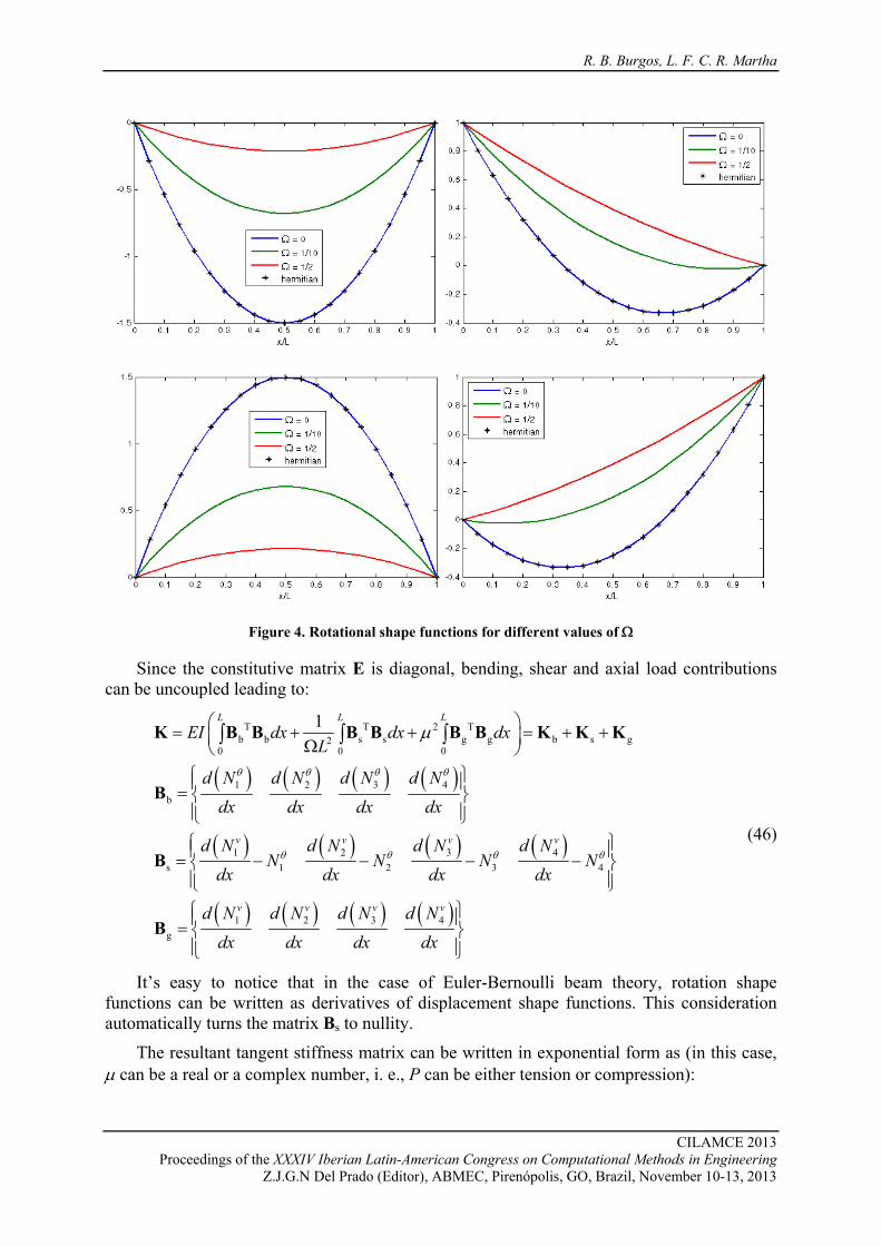
Figure 4. Rotational shape functions for different values of Ω

Since the constitutive matrix E is diagonal, bending, shear and axial load contributions can be uncoupled leading to:

( ) ( ) ( ) ( )

( ) ( ) ( ) ( )

( ) ( ) ( ) ( )

T T 2 Tb b s s g g b s g2

0 0 0

1 2 3 4b

1 2 3 4s 1 2 3 4

1 2 3 4g

1L L L

v v v v

v v v v

EI dx dx dxL


d N d N d N d NN N N N

dx dx dx dx


θ θ θ θ

θ θ θ θ

μ⎛ ⎞= + + = + +⎜ ⎟Ω⎝ ⎠⎧ ⎫⎪ ⎪= ⎨ ⎬⎪ ⎪⎩ ⎭⎧ ⎫⎪ ⎪= − − − −⎨ ⎬⎪ ⎪⎩ ⎭⎧ ⎫⎪ ⎪= ⎨ ⎬⎪ ⎪⎩ ⎭

∫ ∫ ∫K B B B B B B K K K

B

B

B

(46)

It’s easy to notice that in the case of Euler-Bernoulli beam theory, rotation shape functions can be written as derivatives of displacement shape functions. This consideration automatically turns the matrix Bs to nullity.

The resultant tangent stiffness matrix can be written in exponential form as (in this case, μ can be a real or a complex number, i. e., P can be either tension or compression):



( ) ( )( )

( ) ( )

( ) ( )( )( )

( )( )( )

( )

3 2 2

11 33 13 31 3

2

12 21 14 41 23 32 34 43 2

2 2 2 2

22 44

2 2 2

24 42

1 11212

166

1 1 144 1

1 1 222 1

1 2 1

L

L

L L

L

L L

L

L

L L eEIk k k kL D

L eEIk k k k k k k kL D

L L e L eEIk kL D e

L L e LeEIk kL D e

D L e

μ

μ

μ μ

μ

μ μ

μ

μ

μ μ

μ

μ μ μ

μ μ μ

μ μ

+ Ω += = − = − =

−= = = = − = − = − = − =

⎡ ⎤+ − − Ω −⎣ ⎦= =−

⎡ ⎤− Ω − −⎣ ⎦= =−

= + − − Ω( )( )2 2 221 , ,

1

L

c

c

P EIL eGA LPEI

GA

μ μ− = Ω =⎛ ⎞

+⎜ ⎟⎝ ⎠

(47)

In terms of hyperbolic functions, the coefficients become:

( ) ( )

( ) ( )

( ) ( ) ( )

( ) ( )

[ ]

3 2 2

11 33 13 31 3

2

12 21 14 41 23 32 34 43 2

2 2

22 44

2 2

24 42

2

1 senh( )1212

cosh( ) 166

cosh 1 senh44

1 senh22

2 2 cosh( ) 1

L L LEIk k k kL D

L LEIk k k k k k k kL D

L L L L LEIk kL D

L L L LEIk kL D

D L L

μ μ μ

μ μ

μ μ μ μ μ

μ μ μ μ

μ μ

+ Ω= = − = − =

−= = = = − = − = − = − =

⎡ ⎤− − Ω⎣ ⎦= =

⎡ ⎤− Ω −⎣ ⎦= =

= − ⋅ ⋅ − Ω( )2 senh( )L Lμ μ+ ⋅ ⋅

(48)

And in terms of trigonometric functions:

( ) ( )

( ) ( )

( ) ( ) ( )

( ) ( )

[ ] ( )

3 2 2

11 33 13 31 3

2

12 21 14 41 23 32 34 43 2

2 2

22 44

2 2

24 42

2 2

1 sen( )1212

1 cos( )66

1 sen cos44

1 sen22

2 2 cos( ) 1

L L LEIk k k kL D

L LEIk k k k k k k kL D

L L L L LEIk kL D

L L L LEIk kL D

D L L L

μ μ μ

μ μ

μ μ μ μ μ

μ μ μ μ

μ μ μ

− Ω= = − = − =

−= = = = − = − = − = − =

⎡ ⎤+ Ω −⎣ ⎦= =

⎡ ⎤− + Ω⎣ ⎦= =

= − ⋅ ⋅ + Ω − ⋅ ⋅

2

sen( )

1c

L

PPEI

GA

μ

μ = −⎛ ⎞

−⎜ ⎟⎝ ⎠

(49)




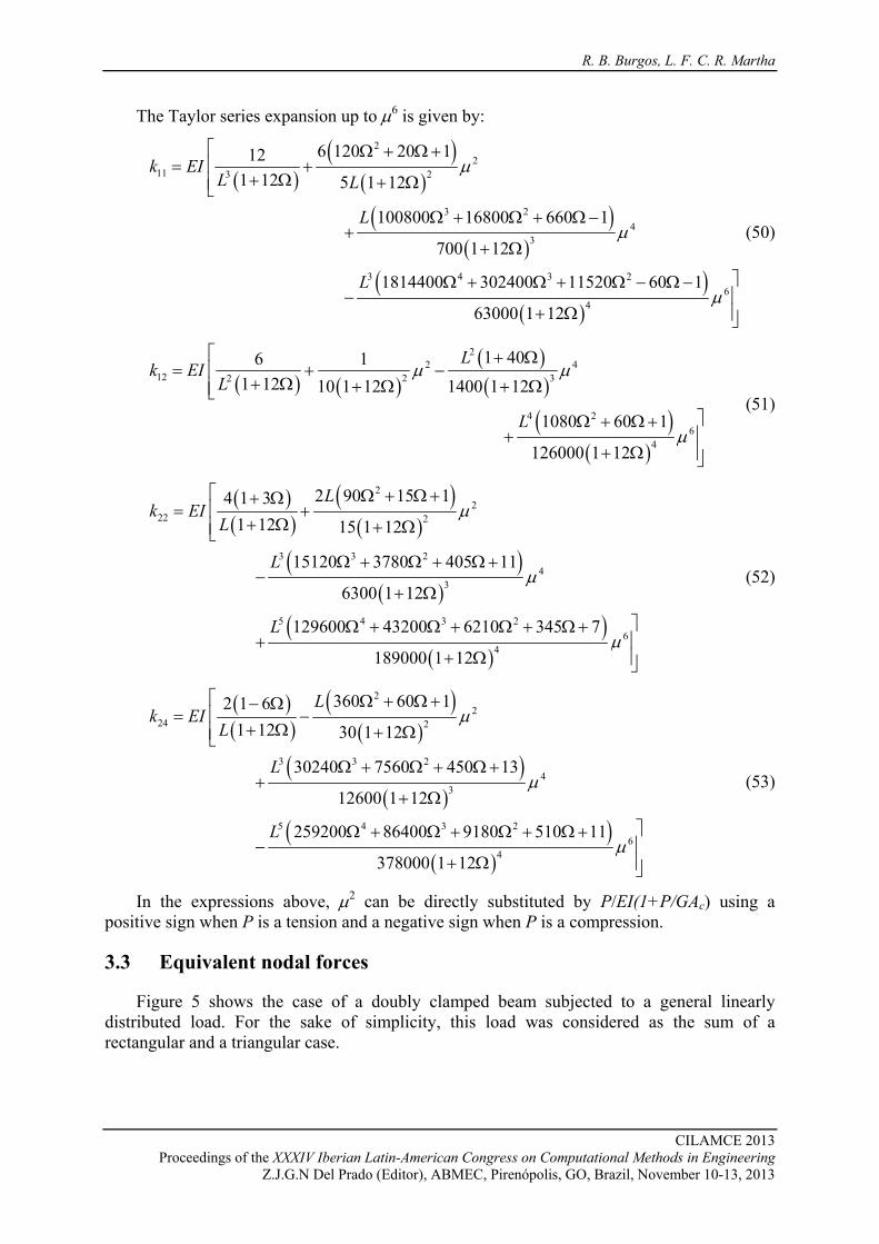
The Taylor series expansion up to μ6 is given by:

( )( )

( )

( )( )

( )( )

22

11 23

3 24

3

3 4 3 26

4

6 120 20 1121 12 5 1 12

100800 16800 660 1

700 1 12

1814400 302400 11520 60 1

63000 1 12

k EIL L

L

L

μ

μ

μ

⎡ Ω + Ω +⎢= +

+ Ω + Ω⎢⎣

Ω + Ω + Ω −+

+ Ω

⎤Ω + Ω + Ω − Ω −⎥−

+ Ω ⎥⎦

(50)

( ) ( )( )( )

( )( )

22 4

12 2 32

4 26

4

1 406 11 12 10 1 12 1400 1 12

1080 60 1

126000 1 12

Lk EI

L

L

μ μ

μ

⎡ + Ω= + −⎢

+ Ω + Ω + Ω⎢⎣⎤Ω + Ω +⎥+

+ Ω ⎥⎦

(51)

( )( )

( )( )

( )( )

( )( )

22

22 2

3 3 24

3

5 4 3 26

4

2 90 15 14 1 31 12 15 1 12

15120 3780 405 11

6300 1 12

129600 43200 6210 345 7

189000 1 12

Lk EI

L

L

L

μ

μ

μ

⎡ Ω + Ω ++ Ω⎢= +

+ Ω + Ω⎢⎣

Ω + Ω + Ω +−

+ Ω

⎤Ω + Ω + Ω + Ω +⎥+

+ Ω ⎥⎦

(52)

( )( )

( )( )

( )( )

( )( )

22

24 2

3 3 24

3

5 4 3 26

4

360 60 12 1 61 12 30 1 12

30240 7560 450 13

12600 1 12

259200 86400 9180 510 11

378000 1 12

Lk EI

L

L

L

μ

μ

μ

⎡ Ω + Ω +− Ω⎢= −

+ Ω + Ω⎢⎣

Ω + Ω + Ω ++

+ Ω

⎤Ω + Ω + Ω + Ω +⎥−

+ Ω ⎥⎦

(53)

In the expressions above, μ2 can be directly substituted by P/EI(1+P/GAc) using a positive sign when P is a tension and a negative sign when P is a compression.

3.3 Equivalent nodal forces

Figure 5 shows the case of a doubly clamped beam subjected to a general linearly distributed load. For the sake of simplicity, this load was considered as the sum of a rectangular and a triangular case.



Figure 5. Linearly distributed load as the sum of two simpler cases

Equivalent nodal forces for a linearly distributed load can be obtained in the following manner:

( ) ( )T T10 1 0 0 x

0 0

10 0 x

0 0

( )

( ) , ( )

L Lv v

L Lv v

i i i i

qxq x q q q dx xdxL L

qf q N x dx f N x xdxL

= + → = + = +

= =

∫ ∫

∫ ∫

F N N F F (54)

After substitution of each shape function:

( ) ( )( )( )( )

( ) ( )( )( )( )

001 03

220

02 04 2 2

220

02 04 2 2

26 senh 2 cosh 1

,12 cosh 1

1

6 sen 2 cos 1,

12 cos 11

c

c

q Lf f

L L Lq L Pf fL L PEI

GA

L L Lq L Pf fL L PEI

GA

μ μ μμ

μ μ

μ μ μμ

μ μ

= =

⎧ ⎫⎡ ⎤− −⎪ ⎪⎣ ⎦= − = =⎨ ⎬− ⎛ ⎞⎪ ⎪⎩ ⎭ +⎜ ⎟

⎝ ⎠⎧ ⎫⎡ ⎤+ −⎪ ⎪⎣ ⎦= − = = −⎨ ⎬

− ⎛ ⎞⎪ ⎪⎩ ⎭ −⎜ ⎟⎝ ⎠

(55)

It’s interesting to notice that equivalent nodal forces are independent of the consideration of shear deformation for a uniformly distributed load. For the linearly distributed part, equivalent loads are:

( )( ) ( ) ( )( ) ( )( )

( )( ) ( )( ) ( ) ( )

( )( ) ( )( ) ( ) ( )( )

2 2 2 2 2 21

x1 2 2

2 221

x2

2 2 2 22

1x4 2 2

10 6 1 6 senh 3 4 1 cosh 1320 9

5 cosh 1 6 2 1 3 3 1 senh

30

10 2 6 1 3 cosh 1 3 3 senh

20 3

L L L L L Lq Lf

L D

L L L Lq Lf

LD

L L L L L Lq Lf

L D

μ μ μ μ μ μ

μ

μ μ μ μ

μ

μ μ μ μ μ μ

μ

⎧ ⎫⎡ ⎤+ − Ω − + − Ω −⎪ ⎪⎣ ⎦= ⎨ ⎬⎪ ⎪⎩ ⎭⎧ ⎫⎡ ⎤− Ω + + Ω − − Ω⎪ ⎪⎣ ⎦= ⎨ ⎬⎪ ⎪⎩ ⎭

⎧ ⎡ ⎤+ − Ω − + − − Ω⎢ ⎥⎣ ⎦= − ⎨

[ ] ( )2 2 22 2 cosh( ) 1 senh( ),1

c

PD L L L LPEI

GA

μ μ μ μ μ

⎫⎪ ⎪

⎬⎪ ⎪⎩ ⎭

= − ⋅ ⋅ − Ω + ⋅ ⋅ =⎛ ⎞

+⎜ ⎟⎝ ⎠

(56)




In terms of trigonometric functions:

( )( ) ( ) ( )( ) ( )( )

( )( ) ( )( ) ( ) ( )

( )( ) ( ) ( )( ) ( )( )

2 2 2 2 2 21

x1 2 2

2 221

x2

2 2 2 2 2 21

x3 2 2

10 6 1 6 sen 3 4 1 cos 1320 9

5 cos 1 6 2 1 3 3 1 sen

30

10 2 3 1 3 sen 3 4 1 cos 1720 21

L L L L L Lq Lf

L D

L L L Lq Lf

LD

L L L L L Lq LfL D

μ μ μ μ μ μ

μ

μ μ μ μ

μ

μ μ μ μ μ μ

μ

⎧ ⎫⎡ ⎤− − Ω + − + Ω −⎪ ⎪⎣ ⎦= ⎨ ⎬⎪ ⎪⎩ ⎭⎧ ⎫⎡ ⎤− Ω + + Ω − + Ω⎪ ⎪⎣ ⎦= ⎨ ⎬⎪ ⎪⎩ ⎭⎧ ⎫⎡ ⎤− + + Ω − + + Ω −⎪ ⎣ ⎦= ⎨⎪⎩

( )( ) ( )( ) ( ) ( )( )

[ ] ( )

2 2 2 22

1x4 2 2

2 2 2

10 2 6 1 3 cos 1 3 3 sen

20 3

2 2 cos( ) 1 sen( ),1

c

L L L L L Lq Lf

L D

PD L L L LPEI

GA

μ μ μ μ μ μ

μ

μ μ μ μ μ

⎪⎬⎪⎭

⎧ ⎫⎡ ⎤− − − Ω − + − + Ω⎢ ⎥⎪ ⎪⎣ ⎦= − ⎨ ⎬⎪ ⎪⎩ ⎭

= − ⋅ ⋅ + Ω − ⋅ ⋅ = −⎛ ⎞

−⎜ ⎟⎝ ⎠

(57)

3.4 Considerations on Ω

Using common relations between elastic constants, considerations on Ω can be inferred.

( )( ) ( )

( )

2

222

, ,2 1

2 1 2 1,

cc

EI EG A AGA L

I IrL A AL

r

χν

ν νχ χ

Ω = = =+

+ +Ω = = =

(58)

In Eq. (58), χ stands for the shear factor and L/r is the slenderness ratio of the beam-column. For rectangular sections, χ = 5/6 and Eq. (58) becomes:

( )

( )2

1

5 Lh

ν+Ω = (59)

Figure 6 shows how Ω decreases with L/h. Poisson ratio is given by ν = 0.3.

Figure 6. Shear constant Ω vs. length-to-height ratio



4 EXAMPLES

As a first example, the critical load for a simply supported column was obtained for different values of Ω. In a second example, Roorda’s frame was used to verify the consistency of the formulation when applied to portal frames considering shear deformation.

4.1 Critical load for a simply supported column

Critical loads for a simply supported beam-column were obtained by finding the value of μ which introduces a singularity in the tangent stiffness matrix (det(K) = 0). Approximate values for critical loads were then obtained using Taylor series expansion of the stiffness coefficients up to the third order. This approach leads to a nonlinear eigenvalue problem.

Exact values for critical loads considering shear deformation are given in Bazant (1991).

( )0 2 2

02 22 20

, ,11

crcr cr

ccr

c

P EI EI EIP PL GA LLP

GA

π ππ

= = − = − Ω =⎛ ⎞ + Ω

−⎜ ⎟⎝ ⎠

. (60)

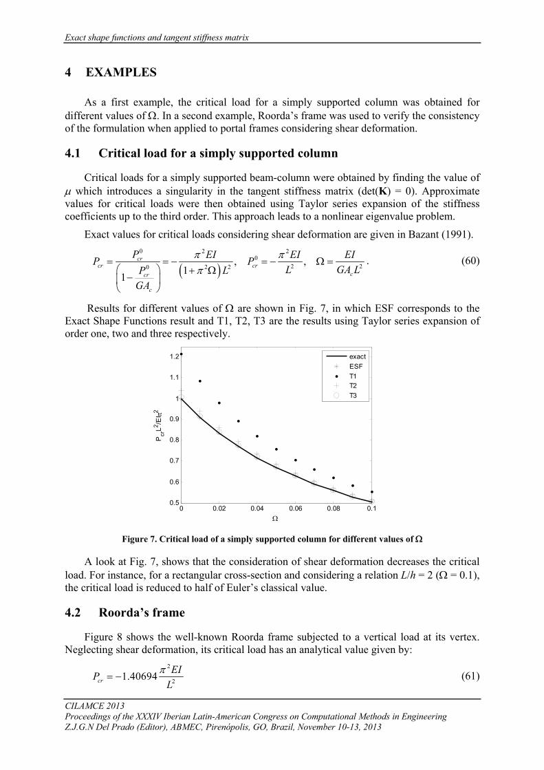
Results for different values of Ω are shown in Fig. 7, in which ESF corresponds to the Exact Shape Functions result and T1, T2, T3 are the results using Taylor series expansion of order one, two and three respectively.

Figure 7. Critical load of a simply supported column for different values of Ω

A look at Fig. 7, shows that the consideration of shear deformation decreases the critical load. For instance, for a rectangular cross-section and considering a relation L/h = 2 (Ω = 0.1), the critical load is reduced to half of Euler’s classical value.

4.2 Roorda’s frame

Figure 8 shows the well-known Roorda frame subjected to a vertical load at its vertex. Neglecting shear deformation, its critical load has an analytical value given by:

2

21.40694crEIP

Lπ

= − (61)

0 0.02 0.04 0.06 0.08 0.10.5

0.6

0.7

0.8

0.9

1

1.1

1.2

Ω

Pcr

L2 /EI π

2

exactESFT1T2T3




Figure 8. Roorda’s frame subjected to a concentrated vertical load

The consideration of shear deformation in this case has a double influence in the critical load, since both bars will experience its effect. Analytically, the critical load can be obtained by solving the following equation:

( ) ( ) ( ) ( )2 2 21 6 3 sin 3 cos 0, 1cr cr cL L L L P EI P GAμ μ μ μ μ⎡ ⎤+ Ω + − = = − +⎣ ⎦ (62)

Figure 9 shows the results for different values of Ω. The double influence is evident since the critical load decreases at a higher rate than observed in the previous example.

Figure 9. Critical load of Roorda’s frame for different values of Ω

5 CONCLUSIONS

This paper presented exact solutions for axially loaded Timoshenko beams. Explicit expressions for shape functions, stiffness matrix and equivalent nodal forces were given. Taylor series expansions were developed in order to compare exact and numerical solutions.

From the examples shown, the different possibilities of approximation can be discussed. Clearly, the first order approximation (which leads to the mostly used geometry matrix) is not reliable in terms of critical loads. A reliable result in this case depends on the experience of the analyst to choose a proper discretization for the model. Higher-order approximations lead to much better results, but with greater computational effort, since critical loads are obtained through the solution of a nonlinear eigenvalue problem. When using the exact element, axial

0 0.05 0.1 0.15 0.2 0.250.2

0.4

0.6

0.8

1

1.2

1.4

1.6

1.8

2

Ω

Pcr

L2 /EI π

2

exactESFT1T2T3



loads cannot be explicitly isolated. The solution in this case is to find the axial load which nulls the determinant of the stiffness matrix. This strategy is also computationally expensive.

In future works, all physically possible combinations of the constants involved will be studied, in order to verify situations in which the general solution doesn’t apply. The treatment of the complete equation, considering Timoshenko beam theory, two-parameter elastic foundation and axial load is still a challenge and will also be a theme of future studies.

REFERENCES

Areiza-Hurtado, M., Vega-Posada, C. & Aristizábal-Ochoa, D., 2005. Second-order stiffness matrix and loading vector of a beam-column with semirigid connections on an elastic foundation, Journal of Engineering Mehanics, pp. 752-762

Bazant, Z. P. & Cedolin, L., 1991, Stability of structures, Dover Pub., NY.

Chiwanga, M. & Valsangkar, A. J., 1988. Generalized beam element on two-parameter elastic foundation, Journal of Structural Engineering, vol. 114, n. 6, pp. 1414-1427.

Eisenberger, M. & Yankelevsky, D. Z., 1984. Exact stiffness matrix for beams on elastic foundation, Computers & Structures, vol. 21, n. 6, pp. 1355-1359.

Morfidis, K. & Avramidis, I. E., 2002. Formulation of a generalized beam element on a two-parameter elastic foundation with semi-rigid connections and rigid offsets, Computers and Structures, vol. 80, pp. 1919–1934.

Morfidis, K., 2007. Exact matrices for beams on three-parameter elastic foundation, Computers and Structures, vol. 85, pp. 1243–1256.

Nukulchai, W. K., Dayawansa & P. H., Karasudhi, P., 1981. An exact finite element model for deep beams, International Journal of Structures, vol. 1, n. 1, pp 1-7.

Onu, G., 2000. Shear effect in beam finite element on two-parameter elastic foundation, Journal of Structural Engineering, vol. 126, n. 9, pp. 1104–1107.

Onu, G., 2008. Finite elements on generalized elastic foundation in Timoshenko beam theory, Journal of Engineering Mechanics, vol. 134, n. 9, pp. 763-776.

Ready, J. N., 1997. On locking-free shear deformable beam finite elements, Computer methods in applied mechanics and engineering, vol. 149, pp. 113-132.

Reddy, J. N., Wang, C. M. & Lee, K. H., 1997. Relationships between bending solutions of classical and shear deformation beam theories, International Journal of Solids and Structures, vol. 34, n. 26, pp. 3373-3384.

Simmons, G. F., 1972. Differential equations with applications, McGraw-Hill.

Shrima, L. M. & Giger M. W., 1992. Timoshenko beam element resting on two-parameter elastic foundation, Journal of Engineering Mechanics, vol. 118, n. 2, pp. 280-295.

Timoshenko, S. P., 1921. On the correction factor for shear of the differential equation for transverse vibrations of bars of uniform cross-section, Philosophical Magazine, pp. 744.

Ting, B. Y. & Mockry, E. F., 1984. Beam on elastic foundation finite element, Journal of Structural Engineering, vol. 110, n. 10, pp. 2324-2339.

Zhaohua, F. & Cook, R. D., 1983. Beam elements on two-parameter elastic foundations, Journal of Engineering Mechanics, vol. 109, n. 6, pp 1390-1402.