A THREE-DIMENSIONAL GRAPHICS APPLICATION FOR NUMERICAL ...webserver2.tecgraf.puc-rio.br/~lfm/papers/Figueiredo-MECOM-CILAMCE... · a three-dimensional graphics application for numerical

A THREE-DIMENSIONAL GRAPHICS APPLICATION FOR NUMERICAL

SIMULATIONS OF TURBIDITY CURRENTS IN THE STRATIGRAPHIC

MODELLING PROCESS

Fabio P. Figueiredoa, Luiz Fernando Marthab and David Walthamc

aTecgraf/PUC-Rio - Computer Graphics Technology Group, Pontifical Catholic University of Rio

de Janeiro, Rua Marques de São Vicente, 225, Gávea, Brazil, [email protected],

http://www.tecgraf.puc-rio.br/~fabiopf

bCivil Engineering Department and Tecgraf/PUC-Rio - Computer Graphics Technology Group,

Pontifical Catholic University of Rio de Janeiro, Rua Marques de São Vicente, 225, Gávea, Brazil,

[email protected], http://www.tecgraf.puc-rio.br/~lfm

cDepartment of Earth Sciencest, Royal Holloway, University of London, Egham, Surrey TW20

0EX, England, [email protected], http://www.rhul.ac.uk/Earth-Sciences

Keywords: Turbidity currents, gravitational flows, numeric simulations, fluid

dynamics, software, object-oriented programming, C++.

Abstract. Turbidity currents occur in both natural and man-made situations. In agreement

with some researchers, most of the world’s oil reserves are stored in hydrocarbon reservoir

built by turbidity systems. Due to the importance of these currents, this work presents a

three-dimensional graphics application for numerical simulations of turbidity currents called

Turb3D. This application is based on a consistent and efficient numerical method for

simulations of turbidity currents for basin sedimentations predictions in the stratigraphic

modelling process. The algorithm used in the software is based on Navier-Stokes equations

that are solved using a depth-averaged procedure. The application user interface provides a

common, user-friendly, graphical environment for pre-processing, solution and post-

processing. Despite the good computational performance achieved by using this approach,

experiments should be done in order to validate the proposed numerical method presented

in this work.

Mecánica Computacional Vol XXIX, págs. 8633-8649 (artículo completo)Eduardo Dvorkin, Marcela Goldschmit, Mario Storti (Eds.)

Buenos Aires, Argentina, 15-18 Noviembre 2010

Copyright © 2010 Asociación Argentina de Mecánica Computacional http://www.amcaonline.org.ar

1 INTRODUCTION

Among the types of transport available in nature, water is by far the most

important transport mechanism. However, this work will concentrate on the

behaviour of a different transport mechanism: density currents. The main difference

between these two mechanisms is that water transports individual sediment particles,

or pieces of rocks, by dragging, saltation or suspension, while density currents consist

of a sediment-fluid mixture that is under the influence of gravity, which explains the

denomination gravity current.

Density current or gravity current occurs in both natural and man-made situations.

Turbidity currents, debris flows, avalanches, oceanic fronts, pyroclastic flows and lava

flows are some examples of this type of current.

Gravity currents are gravitational flows that move according to gravitational forces.

The density difference between both fluids can be caused by thermal effects,

dissolved or suspended material into the current, or by a combination of these two

factors. The current is called conservative if the material is dissolved into the current.

However, if the material is suspended it is called non-conservative.

Gravity currents have been discussed in many scientific studies, especially in

geology. Their importance is due to the fact that these currents have a substantial

influence on the deep-water depositional system. However, density currents can

occur not only in submarine environments but also in subaerial environments.

To generate turbidity currents in a submarine environment, it is indispensable to

have a solution of sediment and water mixture, which has normally a greater density

than the surrounding water. The difference in density between two fluids is the

ignition of gravity currents in general. A difference of only a few percent is enough to

raise the fluid pressure force that together with the fluid weight component (if on a

slope), induce the current to propagate. Based on the Reynolds number, it is possible

to say that this propagation over time, velocity, might affect proportionally the flow

turbulence (Waltham, 2004).

There has been extensive research on theoretical and experimental gravity

currents. These studies have been conducted by many researchers from different

areas with the objective of understanding the dynamics of these currents.

Mathematical modelling of gravity currents can provide significant insights into

current velocity and thickness used to predict turbidite geometries and grain size

distribution. Mathematical models range of forms from simple hydraulic equations

and box models to highly complex turbulence models. In particular, mathematical

models for gravity currents can be divided into four groups: simple model based on

Chézy’s equation, box models, depth-averaged models, and models incorporating

turbulence.

The mathematical model used in this work was based on a depth-averaged

approach. This approach was chosen because it is not as simple as Chézy’s equation

and it is not as complex as models incorporating turbulence, which require more CPU

resources. Despite depth-averaged models unable to model fluid dynamic processes

F. FIGUEIREDO, L. MARTHA, D. WALTHAM8634


within turbidity currents, this choice is arguably the best solution; as it produces

relatively accurate predictions of current evolution and deposition with less demand

on CPU resources.

2 MATHEMATICAL MODEL

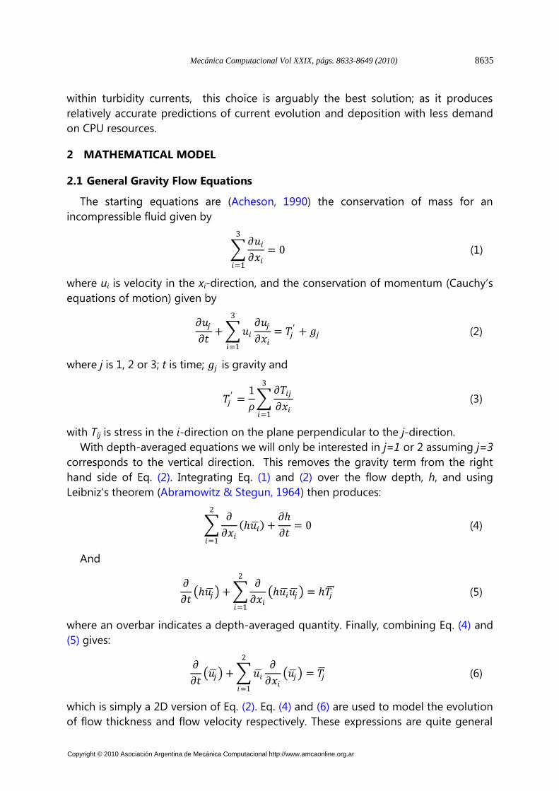
2.1 General Gravity Flow Equations

The starting equations are (Acheson, 1990) the conservation of mass for an

incompressible fluid given by

𝜕𝑢𝑖

𝜕𝑥𝑖

3

𝑖=1

= 0 (1)

where ui is velocity in the xi-direction, and the conservation of momentum (Cauchy’s

equations of motion) given by

𝜕𝑢𝑗

𝜕𝑡+ 𝑢𝑖

𝜕𝑢𝑗

𝜕𝑥𝑖

3

𝑖=1

= 𝑇𝑗′ + 𝑔𝑗 (2)

where j is 1, 2 or 3; t is time; 𝑔𝑗 is gravity and

𝑇𝑗′ =

1

𝜌

𝜕𝑇𝑖𝑗

𝜕𝑥𝑖

3

𝑖=1

(3)

with Tij is stress in the i-direction on the plane perpendicular to the j-direction.

With depth-averaged equations we will only be interested in j=1 or 2 assuming j=3

corresponds to the vertical direction. This removes the gravity term from the right

hand side of Eq. (2). Integrating Eq. (1) and (2) over the flow depth, h, and using

Leibniz’s theorem (Abramowitz & Stegun, 1964) then produces:

𝜕

𝜕𝑥𝑖

2

𝑖=1

𝑕𝑢𝑖 +𝜕𝑕

𝜕𝑡= 0 (4)

And

𝜕

𝜕𝑡 𝑕𝑢𝑗 +

𝜕

𝜕𝑥𝑖 𝑕𝑢𝑖 𝑢𝑗

2

𝑖=1

= 𝑕𝑇𝑗′ (5)

where an overbar indicates a depth-averaged quantity. Finally, combining Eq. (4) and

(5) gives:

𝜕

𝜕𝑡 𝑢𝑗 + 𝑢𝑖

𝜕

𝜕𝑥𝑖 𝑢𝑗

2

𝑖=1

= 𝑇𝑗 (6)

which is simply a 2D version of Eq. (2). Eq. (4) and (6) are used to model the evolution

of flow thickness and flow velocity respectively. These expressions are quite general

Mecánica Computacional Vol XXIX, págs. 8633-8649 (2010) 8635


as they make no assumptions concerning rheological properties (e.g. non-zero

viscosity or yield strength), flow style (e.g. laminar, turbulent or granular) or about

how flow density varies in time and space. These factors only enter via the stress

term on the right hand side of equation (6).

2.2 Stresses in a Turbulent Newtonian Flow

A Newtonian fluid is defined by the stress relationship (Acheson, 1990)

𝑇𝑖𝑗 = −𝑝𝛿𝑖𝑗 + 𝜇 𝜕𝑢𝑗

𝜕𝑥𝑖+𝜕𝑢𝑖

𝜕𝑥𝑗 (7)

where p is pressure and is viscosity. For the turbulent flow case considered in this

paper, velocities should be understood as being ensemble averages (i.e. averages

over a large numbers of identical flows) whilst is the eddy viscosity. For the low-

concentration turbidity current case the flow density is nearly constant (i.e. equal to

water density, w) so that Eq. (3) and (7) yield

𝑇𝑗 ≈1

𝜌 𝜕𝑝

𝜕𝑥𝑗

+ 𝜇∇2𝑢𝑗 + 𝜏𝑗 𝑕 − 𝜏𝑗 0 (8)

where ∇2= 𝜕2 𝜕𝑥12 + 𝜕2 𝜕𝑥2

2 and 𝜏𝑗 = 𝜇 𝜕𝑢𝑗 𝜕𝑥3 is horizontal shear stress in the j

direction.

For a thin flow, in which characteristic horizontal scales are generally much greater

than flow thickness, a hydrostatic approximation is appropriate for calculation of the

pressure gradient in Eq.(8). In addition, for simplicity, we assume that flow

concentration is constant so that

𝜕𝑃

𝜕𝑥𝑗

=

𝜕𝑃

𝜕𝑥𝑗= ∆𝜌𝑔

𝜕𝑕𝑓

𝜕𝑥𝑗 (9)

where is the density contrast between the flow and the ambient fluid and hf is the

height of the flow top.

The eddy-viscosity term in Eq. (8) is formally equivalent to a velocity-diffusion

equation and this therefore simply smoothes the resulting velocity field. The diffusion

coefficient is given by w which depends upon the flow speed and could be

anisotropic. However, for simplicity, we treat this as a constant modelling parameter

chosen to ensure numerical stability.

The horizontal shear stress terms in Eq. (8) can be estimated using mixing-length

theories (Duncan et al, 1960). We can approximate the relatively small contribution to

shear-stress from the flow top by using a multiplier with the basal shear stress. The

next step is to represent the basal stress by an equivalent shearing velocity, 𝑢∗, given

by:

𝜏 = −𝜌𝑢∗2 ≈ −𝜌𝑤𝑢∗

2 (10)



in which the negative sign indicates that stress acts in the opposite direction to the

velocity. Within the turbulent boundary layer, the shearing velocity is related to the

flow velocity by the law of the wall

𝑢 =𝑢∗

𝑘𝑙𝑛

𝑧

𝑧0 𝑧0 < 𝑧 < 𝑧𝑏 (11)

where k is von Kármán’s constant (NB the clear-water value of ~0.41 is unlikely to be

greatly in error for the low-concentration flows considered in this paper), z is height

above channel floor whilst zo and zb define the depth range of the turbulent

boundary layer. Integration of Eq. (11) yields an average velocity over this boundary

layer of

𝑢 𝑏 =𝑢∗

𝑘 𝑙𝑛

𝑧𝑏𝑧0 − 1 +

𝑧0

𝑧𝑏 ≈

𝑢∗

𝑘 𝑙𝑛

𝑧𝑏𝑧0 − 1 (12)

assuming zb>>zo. Above this boundary layer Kneller et al. (1999) showed

experimentally that the velocity profile approximates well to a cumulative Gaussian

function. However, for greater generality as well as mathematical simplicity, the

average velocity in the upper part of the flow can be represented by the velocity at

the top of the boundary layer multiplied by a constant, i.e.

𝑢 𝑡 = 𝑎𝑢 𝑧𝑏 =𝑎𝑢∗

𝑘𝑙𝑛

𝑧𝑏𝑧0 (13)

where tu is the average velocity in the upper part of the flow and a is of order one.

Combining Eq. (12) and (13) then gives a depth-averaged velocity through the

entire flow of

𝑢 = 𝑓𝑢 𝑏 + (1 − 𝑓)𝑢 𝑡

𝑢 =𝑢∗

𝑘 𝑓 + (1 − 𝑓)𝑎 𝑙𝑛

𝑧𝑏𝑧0 − 𝑓

𝑢 =𝑢∗

𝑘𝑏 𝑙𝑛

𝑧𝑏𝑧0 =

𝑢∗

𝑘𝑏 𝑙𝑛

𝑕𝑓

𝑧0

(14)

where f=zb/h is the fractional height of the boundary layer and b = f+(1-f)a is a new

constant of order one. Eq. (10) and (14) then combine to give

𝜏 = −𝜌 𝑘𝑢

𝑏𝑙𝑛 𝑕𝑓𝑧0

2

(15)

which, for the 2D (after depth-averaging) flows used here, may be generalized to

𝜏𝑗 = −𝜌𝑢𝑗 𝑉 𝑘


2

(16)

where V is the depth averaged speed (i.e. 2

2

2

1

2 uuV ). Thus, the basal friction is



controlled by two constants; b which we assume is unity and z0/f, which we show

below to be closely related to the seafloor roughness. Note that this approach to

calculating basal shear stress is formally equivalent to using a Chezy-type friction law

except that the resulting Chezy-coefficient has a weak dependency on flow thickness

and, more importantly, it is directly related to a potentially quantifiable parameter (i.e.

the seafloor roughness).

The depth-averaged gravity current modelling algorithm described above has

been validated by comparison with flume-tank experiments (Bitton et al, 2007).

2.3 Particulate Current Modifications

The preceding algorithm applies to any thin, turbulent gravity underflow and so, to

complete the description, we need to add processes specifically related to sediment

suspension and deposition. Our modelling is concerned with deposition from the

distal parts of the flow so we assume the flow is fully developed in terms of sediment

and ambient-fluid entrainment and that sediment deposition is therefore the

dominant process.

For sediment suspension, the turbulence-generated root-mean-square fluctuations

in vertical velocity should exceed the fall velocity, vk (where k runs over all grain

diameters), (Raudkivi 1998 but see Leeder et al. 2005 for a critique) and laboratory

studies (e.g. Bagnold 1966; Kneller et al. 1999) show that the rms fluctuations are of

similar magnitude to the shearing velocity. An entirely equivalent suspension criterion

is that the Rouse number should be less than 2.5 (Rouse, 1937; Allen, 1997) since this

also leads to the expectation of a suspension threshold when fall-velocity

approximately equals the shear velocity. The sedimentation rate, sk, is therefore zero

for 𝑢∗ > 𝑣𝑘 but equal to ckvk (where ck is concentration of the grain size) when the

flow is stationary. The simplest mathematical model consistent with these end-

members is

𝑠𝑘 = 𝑐𝑘 𝑣𝑘 − 𝑢∗ 𝑢∗ ≤ 𝑣𝑘

𝑠𝑘 = 0 𝑢∗ > 𝑣𝑘 (17)

The still-water fall velocity can be calculated using a large number of different

formulae but, for the first order model described in this paper, Stokes’s Law is

adequate. Each grain diameter is then independently modelled using a modified

form of Eq. (4) which incorporates sediment loss:

𝜕

𝜕𝑥𝑖

2

𝑖=1

𝐿𝑘𝑢𝑖 +𝜕𝐿𝑘𝜕𝑡

= −sk (18)

where Lk is the sediment load associated with grain-size k, i.e.

𝐿𝑘 = 𝑐𝑘𝑕 (19)

Flow thickness is then recalculated using



𝑕 = 𝑐 𝐿𝑘𝑘

(20)

where the total concentration of suspended sediments is assumed to be fixed for

consistency with earlier model assumptions. Note that, as a consequence, flows thin

as they loose sediment rather than become less concentrated.

3 COMPUTATIONAL MODEL

This Section shows the approach used for implementation of the governing

equations presented in the previous section.

3.1 Governing equations solution

The summarised mathematical equations for turbidity current proposed in this

work are given by the following expressions.

𝜕𝑕

𝜕𝑡+

𝜕

𝜕𝑥 𝑕𝑢 +

𝜕

𝜕𝑦 𝑕𝑣 = −

𝑠𝑘𝑐𝑘

(21)

𝜕𝑢

𝜕𝑡+

𝜕

𝜕𝑥 𝑢 2 +

𝜕

𝜕𝑦 𝑢𝑣 = −

1

𝜌

∆𝜌𝑔𝜕𝐻

𝜕𝑥+ 𝜌𝑢 𝑢 2 + 𝑣 2

𝑘


2

(22)

𝜕𝑣

𝜕𝑡+

𝜕

𝜕𝑦 𝑣 2 +

𝜕

𝜕𝑥 𝑢𝑣 = −

1

𝜌

∆𝜌𝑔𝜕𝐻

𝜕𝑦+ 𝜌𝑣 𝑢 2 + 𝑣 2

𝑘


2

(23)

In order to store the mesh variables 𝑕, 𝑢 and 𝑣 a staggered grid scheme was used.

In this scheme the height of the flow, 𝑕, is stored in the centre of the grid cell. The

components 𝑢 of the velocity in the x-direction are stored at the left and right faces

of the grid cells, at a distance of ±∆𝑥 2 from the centre, and the 𝑣 components of

the velocity in the y-direction are stored at the top and bottom of the grid cell, at a

distance of ±∆𝑦 2 of the center.

On a staggered grid the scalar variables (pressure, density, total enthalpy, etc) are

stored in the cell centres of the control volumes, whereas the velocity or momentum

variables are located at the cell faces. This is different from a collocated grid

arrangement, where all variables are stored in the same positions. A staggered

storage is mainly used on structured grids for incompressible flow simulations. Using

a staggered grid is a simple way to avoid odd-even decoupling between the pressure

and velocity. Odd-even decoupling is a discretization error that can occur on

collocated grids and which leads to checkerboard patterns in the solutions (CFD

Online, Harlow & Welch, 1965).

Figure 1 shows a part of the computational domain discretized with staggered grid



scheme. The momentum equation in the x-direction, Eq. (22), is discretized at the

position 𝑖 + 1 2 , 𝑗. Analogously, the momentum equation in the y-direction, Eq. (23),

is discretized at the position 𝑖, 𝑗 + 1 2 . Lastly, the continuity equation, Eq. (21), is

discretized at the point i,j located at the centre of the grid cell.

Figure 1: Staggered grid scheme. The height is stored at the centre of the grid and the components of

velocity are stored at the left, right, top and bottom of the grid cell.

Consider the momentum equation in the x-direction discretization at the finite

differences cell, Figure 2.

Figure 2: Discretization of the momentum equation in x-direction.

The discretization at the point 𝑖 + 1 2 , 𝑗 for the advection and pressure terms are

done using second order central difference.



𝜕𝐻

𝜕𝑥 𝑖+1 2 ,𝑗

≈𝐻𝑖+1,𝑗 − 𝐻𝑖 ,𝑗

∆𝑥 (24)

𝜕

𝜕𝑥 𝑢 2

𝑖+1 2 ,𝑗≈

𝑢 2𝑖+1,𝑗 − 𝑢 2

𝑖 ,𝑗

∆𝑥 (25)

𝜕

𝜕𝑦 𝑢𝑣

𝑖+1 2 ,𝑗

≈ 𝑢𝑣 𝑖+1 2,𝑗 +1 2 − 𝑢𝑣 𝑖+1 2,𝑗 −1 2

∆𝑦 (26)

The terms 𝑢 2𝑖+1,𝑗 , 𝑢

2𝑖 ,𝑗 , 𝑢𝑣 𝑖+1 2,𝑗 +1 2 and 𝑢𝑣 𝑖+1 2,𝑗 −1 2 in Eq. (25) and (26) are

not defined on the grid, and are obtained by linear interpolation of the values of 𝑢

and 𝑣 located at the cell faces. The value of 𝐻 in Eq. (24) is given by the sum of the

deposit thickness, 𝑑, the 𝑧 coordinate of the surface and the flow thickness, 𝑕.

The values of the velocity 𝑣 and the flow thickness 𝑕 also are not defined at the

point 𝑖 + 1 2 , 𝑗 in the last term of the Eq. (22). Then, the velocity 𝑣 at this point is

given by the average of the velocities 𝑣 at the adjacents cell faces.

𝑣 𝑖+1 2 ,𝑗 ≈𝑣 𝑖 ,𝑗−1/2 + 𝑣 𝑖+1,𝑗−1/2 + 𝑣 𝑖 ,𝑗+1/2 + 𝑣 𝑖+1,𝑗+1/2

4 (27)

Finally, the value of the flow thickness 𝑕 at the point 𝑖 + 1 2 , 𝑗 is obtained by the

average of the values located at the centre of the adjacent cell.

𝑕 𝑖+1 2 ,𝑗 ≈𝑕𝑖+1,𝑗 + 𝑕𝑖 ,𝑗

2 (28)

Analogously, the discretization of the momentum equation in y-direction, Eq. (23),

at the point 𝑖, 𝑗 + 1 2 is given according to the points showed in the Figure 3.

Figure 3: Discretization of the momentum equation in y-direction.



As mentioned before for the momentum equation in x-direction, the terms 𝑣 2𝑖 ,𝑗+1,

𝑣 2𝑖 ,𝑗 , 𝑢𝑣 𝑖+1 2,𝑗 +1 2 and 𝑢𝑣 𝑖−1 2,𝑗 +1 2 in Eq. (30) and (31) are also not defined on the

grid, and are obtained by linear interpolation of the values of 𝑢 and 𝑣 located at the

cell faces.

𝜕𝐻

𝜕𝑦 𝑖 ,𝑗+1 2

≈𝐻𝑖 ,𝑗+1 − 𝐻𝑖 ,𝑗

∆𝑦 (29)

𝜕

𝜕𝑦 𝑣 2

𝑖 ,𝑗+1 2

≈𝑣 2𝑖 ,𝑗+1 − 𝑣 2𝑖 ,𝑗

∆𝑦 (30)

𝜕

𝜕𝑥 𝑢𝑣

𝑖 ,𝑗+1 2 ≈

𝑢𝑣 𝑖+1 2,𝑗 +1 2 − 𝑢𝑣 𝑖−1 2,𝑗 +1 2

∆𝑥 (31)

The value of 𝐻 in Eq. (29) is given by the sum of the deposit thickness, 𝑑, the 𝑧

coordinate of the surface and the flow thickness, 𝑕. The average of velocity 𝑢 , Eq. (23),

is given by the average of the velocities at the adjacent cell faces.

𝑢 𝑖 ,𝑗+1 2 ≈𝑢 𝑖−1/2,𝑗 + 𝑢 𝑖+1,𝑗 + 𝑢 𝑖−1/2,𝑗+1 + 𝑢 𝑖+1/2,𝑗+1

4 (32)

The flow thickness, 𝑕, is obtained by the average of the adjacents centre of the

cells grids. See Eq. (33).

𝑕 𝑖 ,𝑗+1 2 ≈𝑕𝑖 ,𝑗+1 + 𝑕𝑖 ,𝑗

2 (33)

The continuity equation, Eq. (21), is calculated using upwind scheme. Upwind

schemes use an solution-sensitive finite difference stencil to numerically simulate

more properly the direction of propagation of information in a flow field. The upwind

schemes attempt to discretize hyperbolic partial differential equations by using

differencing biased in the direction determined by the sign of the characteristic

speeds (Wikipedia, Patankar, 1980). For example, at the point 𝑖, 𝑗 the continuity

equation discretization is given according to the points showed in the Figure 4.



Figure 4: Discretization of the continuity equation derivatives.

The first RHS term of the Eq. (21), which represents the derivative of the function

with respect to 𝑥, is given by:

𝜕

𝜕𝑥 𝑕𝑢

𝑖 ,𝑗≈

𝑕𝑑𝑢 − 𝑕𝑒𝑢

∆𝑥 (34)

where:

𝑕𝑑 = 𝑕𝑖 ,𝑗 , 𝑢 𝑖−1/2,𝑗 < 0

𝑕𝑖−1,𝑗 , 𝑢 𝑖−1/2,𝑗 ≥ 0 (35)

𝑕𝑒 = 𝑕𝑖+1,𝑗 , 𝑢 𝑖+1/2,𝑗 < 0

𝑕𝑖 ,𝑗 , 𝑢 𝑖+1/2,𝑗 ≥ 0 (36)

And the second RHS term, which represents the derivative of the function with

respect to 𝑦, is given by:

𝜕

𝜕𝑦 𝑕𝑣

𝑖 ,𝑗

≈𝑕𝑡𝑣 − 𝑕𝑏𝑣

∆𝑦 (37)

where:

𝑕𝑡 = 𝑕𝑖 ,𝑗+1, 𝑣 𝑖 ,𝑗+1/2 < 0

𝑕𝑖 ,𝑗 , 𝑣 𝑖 ,𝑗+1/2 ≥ 0 (38)

𝑕𝑏 = 𝑕𝑖 ,𝑗 , 𝑣 𝑖 ,𝑗−1/2 < 0

𝑕𝑖 ,𝑗−1, 𝑣 𝑖 ,𝑗−1/2 ≥ 0 (39)

The time discretization of the momentum equations is based on the explicit Euler

method, where all terms involving the velocity are discretized in time 𝑛. Then the



term involving the flow thickness 𝑕 is discretized in time 𝑛 + 1. Thus, after the

calculation of the velocities 𝑢 𝑛+1 and 𝑣𝑛+1, all the variables have been advanced in

time.

The equations are easily calculated in time 𝑛 using explicit methods. However,

these methods present some stability restrictions, which limit the range of values that

can be used for the ∆𝑡. On the other hand, implicit discretizations provide a set of

equations which must be solved together thereby consuming more processing power

to solve them. Therefore, the time discretization of the continuity equation, Eq. (21),

at the point 𝑖, 𝑗 of the grid cell is given by:

𝑕𝑖 ,𝑗𝑛+1 − 𝑕𝑖 ,𝑗

𝑛

∆𝑡≈ −

𝑕𝑑𝑢 − 𝑕𝑒𝑢

∆𝑥+𝑕𝑡𝑣 − 𝑕𝑏𝑣

∆𝑦 −

𝑠𝑘𝑐𝑘

(40)

The time discretization of the momentum equations in the directions of x and y at

the face of the grid cell 𝑖, 𝑗, are obtained by the Eq. (41) and (42), respectively.

𝑢 𝑖+1/2,𝑗𝑛+1 − 𝑢 𝑖+1/2,𝑗

𝑛

∆𝑡

≈ −∆𝜌𝑔

𝜌

𝐻𝑖+1,𝑗 − 𝐻𝑖 ,𝑗

∆𝑥

− 𝑢 2

𝑖+1,𝑗 − 𝑢 2𝑖 ,𝑗

∆𝑥+ 𝑢𝑣 𝑖+1 2,𝑗 +1 2 − 𝑢𝑣 𝑖+1 2,𝑗 −1 2

∆𝑦

− 𝑢 𝑖+1/2,𝑗𝑛 𝑢 𝑖+1/2,𝑗

𝑛 2

+ 𝑣 𝑖+1/2,𝑗𝑛

2

𝑘

𝑏𝑙𝑛 𝑕𝑖+1/2,𝑗𝑓

𝑧0

2

(41)

𝑣 𝑖 ,𝑗+1/2𝑛+1 − 𝑣 𝑖 ,𝑗+1/2

𝑛

∆𝑡

≈∆𝜌𝑔

𝜌

𝐻𝑖 ,𝑗+1 − 𝐻𝑖 ,𝑗

∆𝑦

− 𝑣 2𝑖 ,𝑗+1 − 𝑣 2𝑖 ,𝑗

∆𝑦+ 𝑢𝑣 𝑖+1 2,𝑗 +1 2 − 𝑢𝑣 𝑖−1 2,𝑗 +1 2

∆𝑥

− 𝑣 𝑖 ,𝑗+1/2𝑛 𝑢 𝑖 ,𝑗+1/2

𝑛 2

+ 𝑣 𝑖 ,𝑗+1/2𝑛

2

𝑘

𝑏𝑙𝑛 𝑕𝑖 ,𝑗+1/2𝑓

𝑧0

2

(42)

3.2 Stability

The numerical method stability is obtained using the Courant-Friedreichs-Lewy

condition, also known as CFL condition. This condition represents the relation

between the size of the grid cell, the time step and the inflow velocity, and it ensures

the solution stability of the explicit methods.

This condition declares that the numeric wave should propagate as fast as the



physic wave, which means that the numeric wave velocity ∆𝑥 ∆𝑡 must be at least as

fast as the physic wave velocity 𝑢 , i.e. ∆𝑥 ∆𝑡 > 𝑢 (Osher & Fedkiw, 2002). Thus, the

CFL condition can be written as

∆𝑡 <∆𝑥

𝑚𝑎𝑥 𝑢 (43)

The term 𝑚𝑎𝑥 𝑢 is given by the maximum value of the grid velocity. The Eq.

(43) is usually applied assuming a general number for the CFL constant.

∆𝑡 𝑚𝑎𝑥 𝑢

∆𝑥 =∝ (44)

where 0 <∝< 1. According to Osher & Fedkiw (2002), a good choice is ∝= 0.9 or a

more conservative choice of ∝= 0,5. The CFL condition can also be written as

∆𝑡 𝑚𝑎𝑥 𝑉

𝑚𝑖𝑛 ∆𝑥,∆𝑦,∆𝑧 =∝ (45)

4 OVERVIEW OF THE SOFTWARE

All presented equations were implemented into the software program, Turb3D. It

can be used to simulate the evolution and deposition of low density turbidity currents

using multi grain-sizes. This application has a user-friendly GUI for data entry and

result visualizations, Figure 5.

Figure 5: Turb3D application.

Turb3D require some inputs in order to start a new simulation. The first step is to

define an initial surface. It can be done by pressing the “new” button located at the

toolbar of the application. A new project dialog will then be showed, see Figure 6. In

this dialog a file containing the x,y,z coordinates of the surface is imported. This file

consists of three columns of data. The first column represents the x coordinate of the

surface, the second represents the y coordinate and the third represents de z

coordinate. The size, length and width of the grid are calculated automatically by the



program based on the coordinates information which are read from file.

Figure 6: New project dialog.

Then, it is necessary to define the inflow channel by pressing the “channel” button,

Figure 7. In this dialog the height of the channel is specified along with two points

representing its initial and final coordinates.

Figure 7: Channel dialog.

The current parameters are specified by pressing the “current” button. Then, the

current dialog will be displayed as shown in Figure 8.

Figure 8: Current dialog.

Finally, the sediment parameter is specified as shown in Figure 9. For each grain

size it is necessary to specify the diameter of the grain and the concentration of the

grain in the current. For additional information the grain distribution graph is plotted.



Figure 9: Sediment dialog.

After these steps, the simulation can be processed by pressing the “run” button.

The evolution and deposition of the simulation are rendered in real-time.

4.1 Examples

The numerical model proposed must be validated by experiments in order to

check if the simplifications and assumptions used by this work are valid. In other

words, it is fundamental to verify whether the results obtained by using the

application can produce a good prediction of the evolution and deposition of the

current. Then, two examples of experiments that can be performed in laboratories are

simulated using Turb3D.

Simulations are ran using single-grain-size suspensions at 100 and 150 microns

with concentration of 2% by volume, grain density of 2600 kg/m3 and a 40 l/min

inflow. The initial surface file used was created considering a tank with dimensions of

10 m in length, 5 m in width and a 4 degree slope, which generates a file containing

55 nodes in x-direction and 181 nodes in y-direction for a grid size of 0.05 m. The CFL

constant used was 0.5.

Figure 10 shows the 3D contour plot of the surface deposit generated by the

simulation using single-grain-size at 100 microns. The red colour represents the

maximum values and the blue colour represents the minimum values. For this

example the maximum deposit thickness archived was 26.60 mm.



Figure 10: Single-grain-size at 100 microns simulation.

The 3D contour plot of the surface deposit generated by the simulation using

single-grain-size at 150 microns is shown in Figure 11. Again, the red colour

represents the maximum values and the blue colour represents the minimum values.

For this example the maximum deposit thickness archived was 55.90 mm.

Figure 11: Single-grain-size at 150 microns simulation.

5 CONCLUSIONS

The main objectives of this work are to propose a consistent numerical model for

making predictions of the sedimentation processes in stratigraphic modelling which

requires less CPU resources, and to develop a 3D graphical application for turbidity

currents simulation. Furthermore, its important to note that the proposed numerical



method concentrates only on the simulation of the depositional process and not on

the complete turbulent flow.

The numerical model proposed was satisfactory in terms of computational

resources, it was faster than complex models which can consume days of continuous

processing power to solve a single model. The examples presented were ran on a

computer with a 2.50GHz core duo processor and 2GB of RAM. Each example took

about 35 seconds to complete the simulation process.

Despite the good computational performance achieved by using this approach,

experiments should be done in order to validate the proposed numerical method

presented in this work.

REFERENCES

Abramowitz, M. & Stegun, I.A. Handbook of Mathematical Functions. Dover

Publications, 1965.

Acheson, D.J. Elementary Fluid Mechanics. Clarendon Press, 1990.

Allen, P.A. Earth Surface Processes. Blackwell Science, 1997.

Bagnold, R.A. An approach to the sediment transport problem from general physics.

Professional Paper, 422. US Geological Survey, Washington. 1966.

Bitton, L.F.; Martha, L.F.; Waltham, D.; Keevil, G.; Peakall, J. Validation of Simplified

Mathematical Model for Turbidity Currents. SPE Annual Technical Conference and

Exhibition, 21–24 September 2008, Denver, Colorado, USA. 2007.

CFD Online Available at: www.cfd-online.com (Accessed 24 August 2008)

Duncan, W.J., Thom, A.S.; Young, A.D. The Mechanics of Fluids. Edward Arnold,

London. 1960.

Harlow, F.H. and Welch, J.E. Numerical calculation of time-dependent viscous

incompressible flow of fluid with free surface. Phys. Fluids. 8, 2182, 1965

Kneller, B., Bennett, S.; McCaffrey, W. Velocity structure, turbulence and fluid stresses

in experimental gravity currents. Journal of Geophysical Research, C104, 5381–5391,

1999.

Leeder, M.R., Gray, T.E.; Alexander, J. Sediment suspension dynamics and a new

criterion for the maintenance of turbulent suspensions. Sedimentology, 52, 683–691,

2005.

Osher, S.J.; Fedkiw, R. Level Set Methods and Dynamic Implicit Surfaces.

SpringerVerlag, 2002.

Patankar, S.V. Numerical Heat Transfer and Fluid Flow. Taylor & Francis, 1980

Raudkivi, A. Loose Boundary Hydraulics. Balkema, Rotterdam. 1998.

Rouse, H. Modern conceptions of the mechanics of turbulence. Transaction of the

American Society of Civil Engineers, 102, 436–505, 1937.

Waltham, D. Flow transformations in particulate gravity currents. Journal of

Sedimentary Research, 74(1), 129-134, 2004.

Wikipedia, the free encyclopedia Available at: www.wikipedia.org (Accessed 2 June

2008)



http://www.cfd-online.com/

http://www.wikipedia.org/

Documents

A THREE-DIMENSIONAL GRAPHICS APPLICATION FOR NUMERICAL ...webserver2.tecgraf.puc-rio.br/~lfm/papers/Figueiredo-MECOM-CILAMCE... · a three-dimensional graphics application for numerical