Dynamic weighing calibration method for liquidflowmeters – A new approach
Dissertation
zur Erlangung des akademischen Grades
Doktoringenieur(Dr.-Ing.)
vorgelegt derFakultät für Maschinenbau der
Technischen Universität Ilmenau
von Herrn
Dipl.-Ing. Jesús Jaime Aguilera Menageboren am 16.09.1979 in Durango/Mexiko
Tag der Einreichung: 13.12.2011
Tag der Verteidigung: 14.06.2012
Doktorvater: Univ.-Prof. Dr.-Ing. habil. Thomas Fröhlich / TU Ilmenau
2. Gutachter: Dir. u. Prof. Dr. Roman Schwartz / PTB Braunschweig
3. Gutachter: Univ.-Prof. Dr.-Ing. habil. Tino Hausotte / FAU Erlangen-Nürnberg
urn:nbn:de:gbv:ilm1-2012000461


Danksagung
Danksagung
Die vorliegende Arbeit entstand während meiner Tätigkeit als wissenschaftlicher Angestellter im
Fachbereich „Flüssigkeiten“ der Physikalisch-Technischen Bundesanstalt (PTB) in
Braunschweig.
Sehr herzlich möchte ich mich bei Herrn Univ. Prof. Dr.-Ing. habil. Thomas Fröhlich,
Leiter des Fachgebietes Prozessmess- und Sensortechnik der TU Ilmenau, für die intensive
Betreuung und die Unterstützung bei der Bearbeitung des Themas bedanken.
Mein außerordentlicher Dank gilt Herrn Dir. u. Prof. Dr.-Ing. Roman Schwartz, Leiter der
Abteilung „Mechanik und Akustik“, Dr.-Ing. Gudrun Wendt, Leiterin des Fachbereichs
„Flüssigkeiten“, und Dr.-Ing. Rainer Engel, Leiter der Arbeitsgruppe „Rückführung
Flüssigkeitsmessungen“ für die Gelegenheit und Motivation im Ausführen meiner Doktorarbeit
an der PTB.
Bei Frau Dipl.-Phys. Angelika Täubner, wissenschaftliche Mitarbeiterin im Fachbereich
„Darstellung Beschleunigung und Stoßdynamik“, sowie Herrn Klaus Mittlestädt und Herrn
Andreas Hein aus dem Fachbereich „Flüssigkeiten“ danke ich sehr für Ihre Kooperation und
Unterstützung bei meinen experimentellen untersuchen.
Frau Dr.-Ing. Iryna Marfenko und Herrn Dr.-Ing. Jann Neumann danke ich ebenfalls herzlich für
die hilfreichen fachlichen Hinweise und die Korrektur meines Manuskripts.
Meine große Anerkennung gilt meiner Frau und meiner Familie in Mexiko und der Ukraine, die
mich stets aufgemuntert und unterstützt haben, um meine Doktorarbeit erfolgreich zu vollenden.
Jesús Jaime Aguilera Mena
Zusammenfassung
Zusammenfassung
Das Ziel dieser Doktorarbeit ist es, die ersten Schritte zur Umsetzung einer neuen
Kalibriermethode für Durchflussmessgeräte zu beschreiben. Diese Forschungsarbeit wurde im
Fachbereich „Flüssigkeiten“ der Physikalisch-Technischen Bundesanstalt durchgeführt. Sie
realisiert ein dynamisches Wägeverfahren, welches es ermöglicht, den Massendurchfluss
mehrmals unter stationären und quasistationären Bedingungen zu messen. Eine somit verkürzte
Kalibrierzeit bringt einen wichtigen Vorteil für Durchfluss-Kalibrierlaboratorien, um ihre
Kalibrierkosten, den Energieverbrauch und die Arbeitsbelastung zu reduzieren.
Die vorgeschlagene Kalibriermethode beruht auf einer gründlichen Analyse der Wechselwirkung
zwischen den durchflussinduzierten Kräften im Messprozess und der Dynamik des Wäge-
Systems. Basierend auf dieser Analyse wird anschließend eine Reihe von
Signalverarbeitungstechniken angewandt, um sowohl die Stärke der unerwünschten, durch den
Durchfluss induzierten Kräfte zu verringern, als auch das Messrauschen im Ausgangsignal zu
dämpfen. Damit kann die Messgröße einerseits sehr genau und andererseits auch als Funktion
der Zeit ermittelt werden.
Die Wirksamkeit der neuen Kalibriermethode für Durchfluss-Messgeräte wird durch numerische
und experimentelle Tests validiert. Die Ergebnisse zeigen, dass eine Genauigkeit kleiner als
0,1 % erreichbar ist. Außerdem gibt die vorliegende Arbeit Empfehlungen, wie das
vorgeschlagene Messprinzip zukünftig noch weiter verbessert werden kann.

Abstract
Abstract
The aim of this dissertation is to describe the first steps made towards the realization of a new
calibration method for liquid flowmeters. Such the research work carried out at the liquid flow
department of the Physikalisch-Technische Bundesanstalt implements a dynamic weighing
approach, to estimate the mass flow rate several times under stationary and quasi-steady
conditions, thus shortening the calibration time. The latter statement represents a significant
benefit for flow calibration laboratories, which seek to reduce their calibration costs, energy
consumption, and workload.
The proposed calibration method relies on a thorough analysis of the interaction between the
acting flow-induced forces present in the measurement process, and the dynamics of the
weighing system. Then, a series of signal processing techniques based on such an analysis are
implemented in order to attenuate the magnitude of the undesired flow-induced forces as well as
the embedded measurement noise from the system´s output signal, so the measurand can be
determined as a time-varying state variable.
The effectiveness of this new flowmeter calibration method is validated by a series of numerical
and experimental tests in which, according to their results, it reveals that an accuracy level
smaller than 0,1% is attainable by applying the proposed method. Furthermore, this document
offers a guideline of how to improve the performance of the proposed measurement principle at a
future date.

Contents
CONTENTS
1. INTRODUCTION...................................................................................... 11.1 The importance of fluid flow measurements……….….……….……............ 11.2 Motivation of the research work………………………….………................. 21.3 Structure of the research work………….…………………............................ 2
2. CURRENT SITUATION AND GOAL OF THE RESEARCH WORK.................. 42.1 Definition of mass and volumetric flow………………….…………………. 42.2 Definition of a flowmeter…………………………………..………………... 52.3 Traceability chain of fluid flow measurements…………………………….. 72.4 Working principle of a liquid flow primary standard………….………….… 82.5 Current situation………………..………………………………….………… 11
2.5.1 Gravimetric and volumetric flying start-and-stop
liquid flow primary standard…………………………………………....…. 112.5.2 Gravimetric and volumetric standing start-and-stop
liquid flow primary standard…………………………….……...…………. 122.5.3 Dynamic level gauging volumetric
liquid flow primary standard………………….…………………………… 142.5.4 ISO dynamic gravimetric liquid flow primary standard………………………... 152.5.5 Dynamic weighing liquid flow primary standard
with immersed pipe………………………………………………………. 172.5.6 Dynamic weighing liquid flow primary standard
assisted by an in-line flowmeter………………………………….………… 182.6 The proposed dynamic weighing
liquid flow primary standard……………………………..………….............. 20
3. INPUT SIGNAL, MODELING OF THE DYNAMIC WEIGHINGLIQUID FLOW STANDARD AND THECONNECTING VOLUME EFFECT……………………………………….. 223.1 Input signal....................................................................................................... 24
3.1.1 Collected water mass force........................................................................... 243.1.2 Hydrodynamic force…………………………………………….………... 253.1.3 Buoyancy force……………………………………….…………………. 273.1.4 Total fluid force and its block diagram representation………………………………. 27
3.2 The weighing system and its numerical representation……………………... 28

Contents
3.2.1 Spring force……………………………………………………………... 303.2.2 Inertial force and system total mass…………………………………..…….. 313.2.3 Damping force…………………………………………………………... 323.2.4 1-Degree-of-Freedom motion equation of the weighing system……………...…. 333.2.5 Technical considerations in regards to the modeling
of the weighing system……………………………………………...……. 373.2.6 General representation of the weighing system internal filter
and the discrete time representation of its output signal……………………….. 383.3 The connecting volume effect in liquid flow measurements………………... 42
3.3.1 Accuracy considerations in relation to
the connecting volume effect in dynamic liquid flow measurements……………. 46
4. FILTERING TECHNIQUES FOR THE DETERMINATIONAND ACCURACY OF MASS FLOW RATE (PROCESS MODEL)........................ 494.1 Derivation of a process noise filter for the attenuation of
the hydrodynamic force effect upon the balance output responseand the determination of mass flow rate………………………………..…… 51
4.2 Proposed filter algorithms for an improved mass flow ratecalculation based on the identification andreduction of measurement noise………………………………….....………. 574.2.1 Central moving average filter…………………………………………....… 584.2.2 Least-Mean-Square adaptive filter………………………………………..… 604.2.3 Linear Kalman filter…………………………………………...……...….. 65
4.3 Summary……………………………………………………………………. 73
5. NUMERICAL DETERMINATION OF MASS FLOW RATEAND THE RESPONSE OF THE DYNAMIC WEIGHINGLIQUID FLOW STANDARD.................................................................................... 745.1 Fluid forces acting upon the weighing system (input signal).......................... 755.2 Frequency response of the weighing system……………..…………………. 775.3 Continuous time and discrete time response of the balance………………… 815.4 Hydrodynamic force filter................................................................................ 855.5 Proposed measurement noise filters................................................................. 87
5.5.1 Central moving average filter........................................................................ 875.5.2 Least-Mean-Square adaptive filter.................................................................. 895.5.3 Linear Kalman filter.................................................................................... 915.5.4 Summary................................................................................................... 95

Contents
5.6 The influence of the data sampling frequencyand the low pass filter cutoff frequency upon the mass flow rateestimate values and its measurement accuracy enhancement.......................... 96
6. EXPERIMENTAL RESULTS.................................................................................. 1026.1 Transfer standard used for the liquid flow comparison................................... 1026.2 Data acquisition system................................................................................... 1046.3 Implementation of an accelerometer to detect
the initial time of the measurement process…………………………………. 1056.4 Usage of a non-contact laser displacement sensor to
characterize the water jet impact height……………………………………... 1076.5 Characterization of the weighing system´s stiffness
and damping coefficients................................................................................. 1096.6 Results.............................................................................................................. 111
6.6.1 Hydrodynamic force filter............................................................................. 1126.6.2 Analytical and experimental estimation of the hydrodynamic force....................... 1146.6.3 Estimation of the collected mass force……………………………...……...... 1156.6.4 Time offset correction.................................................................................. 1176.6.5 Summary………………………………………………...……………… 122
7. CONCLUSIONS AND OUTLOOK.......................................................................... 126
NOMENCLATURE.................................................................................... 130
REFERENCES......................................................................................................... 135

Chapter 1
1
1. Introduction
1.1 The importance of fluid flow measurementsLiquid flow measurement technology is an important area of engineering that involves all
industrial sectors wherein fluids, such as water, hydrocarbons, bio-fuels, and so on, are
transported and/or traded. The main purpose of this area consists in providing reliable technology
that can technically assure the amount of fluid flowing through a conduit agrees with the
magnitude claimed by a system or an individual [1].
Flow measurement technology has significantly matured in the past decades because it is an
effective way to commercialize valuable fluids, and it improves the efficiency, quality, and
safety in any industrial or scientific process. Nowadays, the main tasks of this sector are focused
on the development of more precise flow measurement devices, the improvement of flow
calibration rigs in order to characterize flowmeters more accurately, the implementation of new
manufacturing as well as calibration methods that deliver more affordable and reliable flow
metering technologies to the industry.
A liquid flow calibration rig plays a fundamental role in all the tasks mentioned above, as this is
the only system capable to reproduce the unit of flow by itself. The latter is because the flow rate
unit is a derived quantity that is realized by the direct traceability to the fundamental units of
time, mass, length, and temperature. As a remark, such a primary standard can reproduce the
flow unit by either using a weighing approach to obtain mass flow (kg/s), or by dimensional
means to directly obtain the volumetric flow (m³/s). Once the primary standard is under
operation, it can proceed with its final goal of disseminating the measurand by the calibration of
flowmeters in different industry sectors.

Chapter 1
2
1.2 Motivation of the research workThe motivation for carrying out this dissertation is focused on the first steps made towards the
realization of a dynamic weighing method, which estimate the time-varying mass flow rate, and
allows the calibration of liquid flowmeters in a shorter time.
At present, the start-and-stop flowmeter calibration systems define the flow unit as an average
quantity, given by metering the difference between the initial and final quantity of the liquid and
the time taken for such a collection. One of the main goals of this research work is the
development of a measurement principle that allows using the existing gravimetric start-and-stop
flowmeter calibration facilities to determine the flow unit several times within a single
measurement run. This means, a calibration method that will measure the time-varying mass
flow rate (under stationary and quasi-steady flow conditions) by analyzing the fluid-mechanical
system dynamics, and the output signal response of the weighing system. The latter will benefit
the flow calibration laboratories in reducing their calibration time, and thus, the calibration costs,
energy consumption, and work load. Another important goal of this research work is to present
an alternative calibration method that can avoid the bypass valve timing error, which is
considered to be the most striking measurement uncertainty contributor, and one of the most
difficult components to characterize in a start-and-stop flowmeter calibration system.
1.3 Structure of the research workThe following research work is divided into six parts: Chapter 2 for instance presents a general
overview in the field of flow primary standards, and the state-of-the-art proposed by some
national measurement Institutes (NMIs) and calibration laboratories, in regards to weighing and
volumetric calibration methods. Then in Chapter 3, the manuscript depicts the main variables
(input) involved in the measurement process as well as a general numerical representation of the
liquid flow standard. Chapter 4 deals with the derivation and application of the process equation
to calculate the mass flow rate estimate via dynamic weighing as well as the performance
assessment of some filter algorithms to attenuate the measurement noise from the measurand.
The latter is with the aim to make the estimate calculations more accurate. The following part of
this research work (Chapter 5) describes the numerical simulation and sequence of the
measurement process, comprising the input variables of the process, the flow standard response
(system), the estimation of the mass flow rate, and the attenuation of measurement noise from
the measurand.

Chapter 1
3
Thereafter, the document describes in Chapter 6 the components of a prototype flow primary
standard used for the application of this new calibration method. Moreover, it shows a series of
experimental tests made in order to compare and to validate the results given by proposed
calibration method, with those results obtained by a PTB traceable transfer standard.
The final part of this work (Chapter 7) addresses the conclusions and remarks reached after
analyzing the new calibration method, numerically and experimentally. Additionally, an outlook
of the investigation is given in order to underline the advantages and limitations of the proposed
calibration method, and how the current results and experiences could help to improve it.

Chapter 2
4
2. Current situation and goal of the research work
2.1 Definition of mass and volumetric flowThe conservation of mass is a fundamental concept of macroscopic physics, which states that the
amount of mass existing in a defined or arbitrary space can neither be created nor destroyed.
Additionally, the mass is characterized for having two physical properties: its occupying volume
and density. For the case of a fluid mass enclosed in a conduit, it is agreed that its density,
volume, and its shape can move and change within the time domain. Furthermore, in accordance
to the continuity law (Eq. 2.1), it is established that the mass flow rate of a fluid entering INwm
and leaving OUTwm the finite volume tube is the same, as long as the finite volume remains
constant in time [1]. Note that the subindex w is used in the equation below to indicate that the
fluid in use is water.
IN IN OUT OUTIN OUT
w IN wOUT
w w=
m m
u A u A
(2.1)
As a definition, the mass flow rate wm is a process variable in which its magnitude is equal to
arbitrary cross section of the tube A, wherein the fluid mass passes at an average velocity u , and
a density w (Fig. 2.1). Moreover, according to the equation of continuity, if there is a constant
volume flow rate for a given area change (change in pipe size), then the average velocity will
inversely change. On the other hand, the volumetric flow rate through the pipe (finite volume)
can be calculated by just multiplying the cross section area of the pipe A, and the average
velocity at that location, as shown in Eq. 2.2.
wV = u A (2.2)
Fig. 2.1 The mass/volume flow rate relationship to the tube cross sectional area and average fluid
velocity

Chapter 2
5
2.2 Definition of a flowmeterA flowmeter is a device that measures the flow rate or the quantity of moving fluid in a closed
conduit, and it consists of primary and secondary elements. The flowmeter primary element is
a device mounted externally or internally to the fluid conduit. Therefore, it can produce a
signal that has a defined relationship to the fluid flow. The latter is in accordance with known
physical laws, which relate the interaction of the fluid with the presence of the primary
element. The secondary element is the part of the flowmeter that receives a signal from the
primary element and displays, records, and/or transmits it as a measure of either mass or
volumetric flow rate [2,3].
For the sake of explanation, the turbine flowmeter can be used to illustrate in practical terms the
tasks of these two elements. In Fig. 2.2, the turbine flowmeter depicts a multi-bladed rotor
(primary element) located in the central part of the fluid stream, so as the fluid impinges on the
blades, this causes the rotor to spin at an angular velocity approximately proportional to the flow
rate [4].
Each of these blades has an embedded ferromagnetic element in order to form a magnetic circuit
with the permanent magnet and pickoff coil (secondary elements) in the meter housing [5]. Then,
the voltage induced in the coil has the form of a sine wave whose frequency is proportional to the
angular frequency of the blades. Thereafter, the output signal is passed through a signal
conditioner in order to have a constant amplitude square wave signal of variable frequency.
Finally, such a square wave frequency signal and a meter factor are used to calculate the flow
rate.
Fig. 2.2 Example of primary and secondary elements of a flowmeter (turbine) [3, 5]

Chapter 2
6
The meter factor is a value used to scale the reading of a flowmeter into a quantity that
corresponds to the current magnitude of the measurand flow rate. Such a factor is determined
when comparing the flow metering device output signal to a flow calibration rig (flow standard)
of known accuracy and measurement uncertainty.
As for the different types of flowmeters, Table 2.1 presents a classification chart, wherein the
flow metering devices are divided into three groups depending on their sensing principle. These
are: mass, volume, and differential pressure.
As the name suggests, the mass and volumetric flowmeters are based on the measurement of
motion of mass or a volume quantity in a defined time. On the other hand, the measurement
principle of the differential pressure flowmeters is based on the pressure difference between
the upstream and downstream side of the meter (caused by the contraction/expansion of the
fluid), and its proportional response with the flow passing through the meter. The
determination of flow rate by means of using differential pressure flowmeters is given by a
theoretical equation, in which the dimensions and geometry of the meter body are taken into
account, as well as the pressure, temperature and fluid density. Additionally, the calculation is
corrected by an experimental factor called the discharge coefficient, which aims to include the
frictional flow factor, and a more realistic magnitude of the cross section area of the fluid into
the equation [4,6]. As a remark, the quantity yield by the differential pressure flowmeters can
be either calculated as mass or volumetric flow rate, as long as the fluid density is known.
Mass Volume Differential pressure
Thermal flowmeterPositive
displacementflowmeter
Orifice plate
Angular momentumflowmeter
Turbine flowmeter Venturi nozzle
Coriolis flowmeter Vortex flowmeter Sonic nozzleElectromagnetic
flowmeterVariable area flowmeter
(Rotameter ®)
Ultrasonicflowmeter
Pitot tube
Laminar flow element
Table 2.1 Flowmeter classification [7]

Chapter 2
7
Despite the given classification of flowmeters listed in Table 2.1, one must be aware that each
of those metering devices works with different physical principles, construction designs, fluids,
and installation conditions. A further description of this topic can be found in: Spitzer´s [5],
Baker´s [7], and Miller´s [8] flow measurement handbooks.
2.3 Traceability chain of fluid flow measurementsIn order to ensure the accuracy level of a flowmeter in a measurement process, it is necessary
first to calibrate the device periodically against either a national flow standard or an accredited
flow calibration rig. Thus, after the calibration [9] has been carried out, the characterized
flowmeter can claim to be traceable [10]. By definition, traceability means that the result of a
flow measurement, no matter where it is made, can be related to a national flow measurement
standard as long as the so called traceability chain is not broken, and each of the different
standards involved have a stated uncertainty.
This concept can be exemplified in Fig. 2.3, wherein national flow standards have direct
traceability to the fundamental standards of mass, time, temperature and length, which are
necessary to define the flow unit. As shown in Fig. 2.3, such standards are located at the top of
the diagram, in order to emphasize their highest level of measurement accuracy. Moreover, for
the sake of metrological assurance, the national flow standards must undergo a periodical
measurement comparison program among other national flow labs with similar accuracy (i.e.,
NEL in the UK, NIST in the USA, and PTB in Germany), with the aim to ensure that the flow
unit is disseminated with the claimed measurement uncertainty [11].
Then, below the national standards are linked the state-approved primary and secondary flow
standards, which feature the lowest measurement uncertainty that a private calibration laboratory
or flowmeter manufacture can achieve. Finally, at the bottom of the diagram are the flowmeters
or flow measuring rigs, which hold a relatively low measurement accuracy (compared to the two
previous groups) but acceptable for industrial process applications. Note that the combined
measurement uncertainty level attained after calibrating the flowmeter will eventually depend on
the linearity, repeatability, reproducibility of the meter itself [12], but also in great part of the
standard used to characterize the measuring device.

Chapter 2
8
Fig. 2.3 Flow traceability chain and the hierarchy of measurement standards [13]
2.4 Working principle of a liquid flow primary standardOne very important characteristic of a primary flow standard already recalled in text is that
unlike secondary and working standards, the primary standard is capable to reproduce the flow
unit by itself, without reference to some other standard of the same quantity (but only to the
fundamental units) [12].
In terms of its conceptual design (Fig. 2.4), the primary flow standard is a hydraulic circuit in
which the liquid is driven by a pumping system, and a control valve is responsible of setting up
the operational flow rate as well as keeping it quasi steady during a calibration. Then, the
pumped liquid circulates through a pipeline of different diameter sizes and geometries, with the
goal to transfer the fluid from the meter under calibration to the mass or volume reference
standard.

Chapter 2
9
The Meter Under Calibration (MUC) section shown in Fig. 2.4 is a straight pipeline, which holds
the flowmeter to be calibrated and is long enough to allow the flow profile to be swirl-free [7]. In
some cases, due to high flow disturbances caused by the upstream fittings (i.e. valves), and/or
limited space to install a long pipeline, a flow straightener is used in order to guarantee an
uniform fully developed turbulent flow profile.
Fig. 2.4 Schematic diagram of the main components of a liquid flow primary standard
Once the circulating fluid passes the flowmeter, it is discharged by a bypass valve into a mass or
volume reference standard for effects of flow calculation. Thereafter, when the reference
standard reaches a certain level, the fluid is re-directed into a supply tank to continue the liquid
circulation. The outcome from this process is either an average flow rate resulting from the
totalized mass Totalm or volume TotalV contained in the reference standards and the time Totalt taken
to collect such an amount of fluid (Eq. 2.3 and Eq. 2.4).
Total
Totalw
mm =t
(2.3)
Total
Totalw
VV =t
(2.4)

Chapter 2
10
The mass flow rate can be converted into volumetric flow rate (or vice versa) if the fluid
density is known. In this case, a relationship between the liquid temperature and its density is
developed for this purpose by means of analyzing the density of a liquid sample at different
temperatures, consulting some standard temperature-density tables, or by installing an online
densitometer [14].
The calibration of flowmeters by using primary flow standards is based on the principle of mass
conservation applied to a control volume. The conservation of mass principle here states that
over a time increment, the change in the mass/volume contained in the reference standards is
equal to the mass/volume that flows through control volume defined by: the MUC, the
connecting pipe, and the mass/volume reference standard.
When performing a calibration, the primary flow standard must provide the most stable
conditions in terms of flow, temperature, and pressure, so that the MUC cannot be highly-
influenced by the pulsatile flow [2], fluid density gradients due to temperature variations and so
on. The ambient temperature is also an important process parameter in order to avoid slight
changes on the calibration factor due to the thermal expansion/contraction of the flowmeter body
(i.e. flowmeter internal diameter).
In some cases, the primary flow standards are equipped with heat exchangers in order to keep the
fluid temperature as constant as possible [14], and/or an air conditioning system to avoid large
temperature gradients among the MUC, connecting pipe, and the mass/volume reference
standards.
During the operation of a dynamic liquid flow primary standard is rather important to keep the
best possible conditions of quasi-steady and quasi-stationary flow and temperature, in order to
calibrate a flowmeter [15]. In this instance, the term quasi-steady flow implies a flow, wherein
the fluid temperature, pressure, and cross section area of the pipe may differ from point to point,
but the flow will slightly change with time. On the other hand, the term quasi-uniform flow
stands for the fluid velocity, which is nearly equal at all points along the straight and constant
cross section area of the meter-under-calibration pipeline.

Chapter 2
11
If a fully steady uniform flow were achieved by a liquid flow primary standard, the dynamic
measurements would be simply assumed to be the same at all times, and at any point of the
pipeline, and therefore equal to a mean value. In practice, this is not the case because, the flow is
in a turbulent regime, the pumping system and pipe fittings produced an inherent pulsating flow,
fluid temperature gradients are mostly present in the system, and so on.
2.5 Current situationThere are different approaches for the realization of the measurand flow. Table 2.2 serves as a
guide for the classification of the primary standards, categorizing the facilities by static and
dynamic, and subdividing them into gravimetric and volumetric. The dynamic weighing primary
standard is the new calibration approach, in which this investigation is concentrated on. The
accuracy issues of these types of facilities are not included in the classification, because the
metrological features of a standard depend upon the calibration requirements, and the
technological capabilities of each flow laboratory. A general description of each calibration
approach is given in the following sections.
Table 2.2 Classification of liquid flow primary standards [16]
2.5.1 Gravimetric and volumetric flying start-and-stop liquid flow primary standard
This type of primary standards (gravimetric and volumetric) comprise three main components for
the determination of flow rate: a bypass valve also known in the flow metrology field as a

Chapter 2
12
diverter valve [17], a collection vessel, and either a balance or a calibrated volumetric tank for
the determination of mass or volumetric flow rate, respectively (Fig. 2.5).
The method of operation consists in measuring the initial vessel mass or the volume before the
filling of liquid starts. At the same time, the fluid circulates through the system, until flow
reaches a quasi-steady flow condition (a). This requirement is mandatory for the accurate
measurement of flow rate, and thus, a reliable characterization of the MUC. When process
conditions are stable, a trigger signal is sent to activate the diverter valve, and thus driving the
liquid into the vessel, and to start counting the collection time by means of a timer (b). When a
certain amount of fluid is gathered into the weighing vessel or the volumetric tank, a second
trigger signal is sent to re-direct the liquid flow back to the supply tank, and to stop the timer (c).
Once the collected water reaches an equilibrium condition, the totalized mass or volume of liquid
is measured and divided by the collection time, in order to obtain the average mass or volumetric
flow rate [5,18].
Fig. 2.5 Gravimetric and volumetric flying start-and-stop primary standard
Chapter 2
13
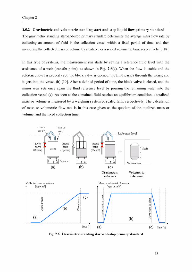
2.5.2 Gravimetric and volumetric standing start-and-stop liquid flow primary standard
The gravimetric standing start-and-stop primary standard determines the average mass flow rate by
collecting an amount of fluid in the collection vessel within a fixed period of time, and then
measuring the collected mass or volume by a balance or a scaled volumetric tank, respectively [7,18].
In this type of systems, the measurement run starts by setting a reference fluid level with the
assistance of a weir (transfer point), as shown in Fig. 2.6(a). When the flow is stable and the
reference level is properly set, the block valve is opened; the fluid passes through the weirs, and
it gets into the vessel (b) [19]. After a defined period of time, the block valve is closed, and the
minor weir sets once again the fluid reference level by pouring the remaining water into the
collection vessel (c). As soon as the contained fluid reaches an equilibrium condition, a totalized
mass or volume is measured by a weighing system or scaled tank, respectively. The calculation
of mass or volumetric flow rate is in this case given as the quotient of the totalized mass or
volume, and the fixed collection time.
Fig. 2.6 Gravimetric standing start-and-stop primary standard

Chapter 2
14
For this kind of facility (either gravimetric or volumetric), it is essential to assure that the amount
of fluid passing through the MUC is the same as for the mass or volume reference standard, so
the continuity law can be applied.
Therefore, in order to accomplish this main requirement, particular attention is paid in the design
of weirs, which can guarantee that the start and stop reference levels triggered by the stop valve
coincide before and after the calibration run (Fig. 2.6(a) and Fig. 2.6(c)).
2.5.3 Dynamic level gauging volumetric liquid flow primary standard
This dynamic level gauging volumetric primary standard, also known as a piston prover [7] is
described as a circular cylinder of a known and uniform internal diameter, which encompasses a
sealed piston (Fig. 2.7). The determination of flow rate is based on the measurement of the fluid
volume out of the cylinder, which is equal to the product of the piston displacement ( Pistonx ) and
the crossed section area ( PistonA ), and the time taken for the piston to travel from one reference
point to another ( Pistont ) [20, 21]. Alternatively, the volumetric flow calculation by a piston
prover can be also seen as the product of the piston velocity ( Pistonx ), and the crossed section area
of the cylinder.
In practical terms, the piston prover operation [22] is graphically depicted in Fig. 2.7(a). At the
initial stage of the measurement (a), the poppet valve of the piston is opened to allow the
circulation of fluid through the cylinder, until quasi-steady flow conditions are achieved. The
measurement of flow rate starts when the poppet valve is closed and the piston is driven forward.
During the first stage of the stroke, the piston undergoes acceleration due to the inertial force of
the downstream fluid illustrated in Fig. 2.7(b). This is considered to be a small region wherein
the flow is suddenly increased, so that, it is preferred to skip it from the measurement process.
Shortly thereafter, the piston acceleration reduces basically to zero [23] and its velocity is fairly
constant, the actuator reaches the start switch and the calibration time begins (Fig. 2.7(b)).
Within the region of measurement, the length scale (linear encoder) is responsible for tracking
the displacement of the piston, and the system keeps time-stamped record for each length step.
At the last stage of the measurement, the actuator approaches the stop switch, which sends the
order to stop the timer, and to open the poppet valve (c).

Chapter 2
15
Fig. 2.7 Dynamic level gauging primary standard (Piston prover) [19]
2.5.4 ISO dynamic gravimetric liquid flow primary standard
At present, some of the liquid flow primary standards operate under the ISO definition of a
dynamic gravimetric liquid flow calibrator [18]. The main reason that encourages some primary
flow laboratories for the implementation of this method is to avoid the tedious characterization of
a bypass valve (diverter valve) [17], which is not longer required since the mass flow rate is
determined by the time taken to match the magnitude of a reference mass with the magnitude
given by the balance readout. This procedure is quite different to the static principle, which
considers the totalized liquid mass and the time taken to collect it.

Chapter 2
16
In this type of facility, exemplified in Fig. 2.8 [24], the liquid circulates until the flow is stable,
and a reference mass named as ISOm is placed upon the balance platform (a). As soon as the
quasi-steady flow condition is achieved, the drain valve is closed, and the liquid starts being
collected in the vessel (b). At some point during the filling, the collected liquid reaches a pre-set
initial mass denoted as Tr1m , and triggers a timer to begin the flow measurement (b). The liquid
continues being poured into the vessel until the fluid matches a second pre-set mass Tr2m , which
generates a trigger signal to lift the reference mass from the balance platform but carrying on
with the filling process (c). Finally, after some time during the collection, the pre-set initial mass
Tr1m is reached once again, and it gives the order to stop the timer as well as the filling process (d).
Thereafter, the average mass flow rate is calculated as the quotient of the reference mass ISOm ,
and the period of time between the triggering points ISOt [25].
The illustration of this type of liquid flow primary standard (Fig. 2.8) is based on an electronic
load cell as a weighing system. On the other hand, mechanical calibrators based on a lever
mechanism are also available for the determination of the flow unit [26, 27], and work under the
same ISO measurement principle depicted in the mass-time and flow-time graphs below.
Fig. 2.8 ISO dynamic gravimetric primary standard

Chapter 2
17
In the last paragraph is written the term average is used because despite this primary standard
operates during the filling process, it still relies on a reference mass for the calculation of a single
mass flow rate measurement, and it disregards the fluctuations of flow rate during ISOt .
2.5.5 Dynamic weighing liquid flow primary standard with immersed inlet pipe
This primary standard developed by the company Rota Yokogawa [28] features four main
components in its design: a weighing system, a flow control valve, a collection vessel, and an
immersed inlet pipe (Fig. 2.9). Unlike the recalled liquid flow calibrators, this primary standard
deals with the minimization of the flow-induced force effect upon the weighing system response,
so that the mass flow rate can be determined as a instant quotient of the balance readout and
time.
The first step of this measurement process is related to the designation of the operational mass
flow rate, taking into account that before starting a calibration run, the flow must be set at a
quasi-steady condition. Once the set up conditions are achieved, the filling process can take
place.
The second step addresses an inherent design problem, which is the counter pressure exerted by
the collected liquid to the discharging flow at the pipe outlet (Fig. 2.9). If this problem were not
treated, the primary standard would simply undergo a continuous decrement of mass flow rate,
and therefore a flowmeter calibration would be impossible to be carried out.
The solution found in order to overcome this problem is the installation of a flow control valve [26],
which can overcome in real time the increasing counter pressure at the pipe outlet, and hence,
assuring a nearly constant pressure and mass flow rate along the filling process.
Another remarkable part in the design of this primary standard is its ability to mechanically
attenuate the normal impacting force caused by the water jet. The mechanical concept consists in
placing inside the vessel, a vertical inlet pipe, which supplies the water mass flow, and it does
not have any contact with the vessel structure (Fig. 2.9). At the pipe outlet, a deflecting plate is
attached with the objective to redirect the normal fluid force into a radial direction, so that, the
water stream will spread out to the side walls of the vessel. The advantage of this application is a
radial fluid force that has a lower effect on the weighing system vibration and balance output

Chapter 2
18
signal, in addition to a faster dissipation of the water jet kinetic energy when spreading the water
throughout the collected water [29]. The other fluid forces taking place in the process are the
product of the continuous increment of liquid mass (desired output quantity), and the local
acceleration of gravity.
Finally, the measurand mass flow rate is calculated in a differentiation form between the balance
readout and time m(t) . The hat symbol on the liquid mass variable is added to indicate that the
magnitude given by the weighing system is a close estimation of the real time-varying mass flow
rate. If none flow-induced forces were present at all in the process, the balance readout would be
equal to the time-varying liquid mass.
Fig. 2.9 Dynamic weighing liquid flow primary standard with immersed inlet pipe
2.5.6 Dynamic weighing liquid flow primary standard assisted by an in-line flowmeter
The U.S. National Institute of Standards and Technology (NIST) has proposed a dynamic
weighing concept for the calibration of liquid flowmeters, which uses the same provisions as for
a conventional static weighing system [30] (a collection vessel, a weighing system, and a bypass
valve), in addition to a flowmeter.
Such a dynamic flow measurement procedure can be described by the following sequence. First,
a calibrated flowmeter is installed upstream the reference weighing system, as illustrated in

Chapter 2
19
Fig. 2.10. Then, after the flow reaches a certain flow stability criterion, the bypass valve drives
the fluid stream into the collection vessel to start the filling process. During the collection, a data
acquisition system records the three main process variables: the output signal of the weighing
system, the flowmeter output signal, and time. The measurement run finishes as soon as the fluid
level matches a preset value defined by the user.
The criterion employed for the calculation of dynamic mass flow rate is divided into two parts:
the rough estimation of mass flow rate and the time-varying flow correction. The rough
estimation of mass flow rate is in this instance, the quotient of the difference between the two
fluid forces measured by the weighing system at a time tn and tn+1, and the local acceleration of
gravity. At this stage of the mass flow calculation, the influences of the water jet impact force as
well as the dynamic response of the weighing system have not yet been treated [31]. Therefore,
the calculated measurand is significantly affected in terms of its precision and accuracy.
Fig. 2.10 Dynamic weighing liquid flow primary standard assisted by an in-line flowmeter
The second part of the process model deals with the precision and accuracy issues mentioned in
the last paragraph, by analyzing separately the error attributed to the dynamic response of the
weighing system and the error originated by the water jet impact force. In order to overcome the
influence of the weighing system dynamics upon the flow measurement, such a primary standard
uses a flowmeter as an alternative form to correct the imprecision of the mass flow rate

Chapter 2
20
estimation. In other words, during a measurement run, the reference flowmeter delivers a value,
which is assumed to follow the time-varying mass flow rate [32]. On the other hand, the
unwanted force magnitude of the water jet impact force (which affects the measurement
accuracy) is estimated by an experimental function relating the water jet impact height, the
weighing system readout, mass flow rate (given by the flowmeter), and time.
2.6 The proposed dynamic weighing liquid flow primary standardThe characteristics of this new liquid flow calibration approach will be described in full detail in
Chapter 3 and Chapter 4. However, at this point it is appropriate to mention some unique
features of the proposed primary standard as well some similarities with its above mentioned
counterparts. For instance:
Unlike the static primary standards and the ISO-based dynamic standard, the calibration time
by the proposed primary standard will be reduced, because the flow unit can be reproduced
several time during a single collection (Section 1.2),
The fast actuation and thorough characterization of a diverter valve is not longer required,
since the measurand is a function of the system dynamics and flow-induced force, and not a
function of a totalized amount of mass and time,
For the static primary standards as well as the ISO-based dynamic standard, the time-varying
mass flow rate is considered as an uncertainty contributor. For the proposed dynamic
weighing liquid flow primary standard, the time-varying mass flow rate is an inherent
characteristic of the measurand,
The effect of fluid evaporation in the proposed primary standard will be relatively low, due to
the fact that the measurement is carried out in a shorter time, in comparison to the static
primary standards,
The proposed dynamic weighing liquid flow primary can be implemented into a conventional
static-weighing liquid flow calibration system, and it does not imply any changes in its
mechanical design.

Chapter 2
21
In order to summarize all the recalled information, Table 2.3 offers an overview of the
measurement approaches for liquid flow, and a way to compare them (in terms of their
advantages and limitations) with the proposed dynamic weighing liquid flow primary standard.
Stat
icw
eigh
ing
+di
vert
er
Stat
icw
eigh
ing
Lev
elga
ugin
g+
dive
rter
Lev
elga
ugin
g
ISO
dyna
mic
wei
ghin
g
Dyn
amic
leve
lga
ugin
g
Dyn
amic
wei
ghin
g
Measurement type Mass Volume Mass
Average flow rate Yes Yes Yes Yes Yes Yes Yes
Time-varying massflow rate
No No No No No Yes Yes
Time of calibration Long Long Long Long Medium Short Short
Fluid and mechanicalinfluences
Diverter error Yes No Yes No No No No
Flow-inducedforcedisturbance
No No No No Medium Low High
Connecting pipe Medium Medium Medium Medium Medium Medium Medium
Fluid evaporation Medium Medium Medium Medium Medium No Low
Flow instability Medium High Medium High Medium Low Medium
Air buoyancy effect Low Low Low Low Low No Low
Temperature variation Medium Medium Medium Medium Medium High Low
Mass Volume
Table 2.3 Characteristics of different liquid flow primary standards

Chapter 3
22
3. Input signal, modeling of the dynamic weighing liquid flow
standard, and the connecting volume effect
As a starting point of this research, it must be stated that the input signal of the measurement
process is a fluid force quantity. However, in order to make present the force quantity in this
dynamic process, it is necessary to produce fluid motion. Therefore, the mass flow rate wm (t) is
in this instance the core variable, or command input of the system [1]. For the sake of early
clarification, it is important to explain that mass flow rate is also the desired output signal of the
measurement process. However, due to the undergoing dynamic conditions in the liquid flow
standard, the system is unable to directly yield the measurand but an estimate value of wm (t) (the
subindex w denotes water as a fluid in use). The term of estimate measurand is used to remark
that in practice, despite the treatment of fluid forces and the system instrumentation, part of the
magnitude of these variables will be unavoidably present in the measurand. Such fluid forces
present in the liquid flow standard are described in the following sections of this chapter, with
the purpose to understand their relevance in the measurement process, and ultimately, its impact
upon the measurand.
Fig. 3.1 describes in a block diagram the dynamic weighing liquid flow standard, wherein its
working principle is explained by three series-connected subsystems. The command input is in
this case the mass flow rate wm (t) . Then, the command input enters the first subsystem called
input elements. Such a block of input elements represents the summation of different mass
flow-induced fluid forces TF (t) that will interact with the next subsystem, the weighing system
(or balance). This second subsystem deals with the mechanical dynamic response of balance, and
the effect of such a behavior upon the fluid force measurement. The third subsystem known as
process model has the task to dynamically estimate the mass flow rate magnitude w nm (t ) based
on an inverse-problem approach [2]. In this case, the inverse-problem approach takes into
account the process parameters from the two previous subsystems (defined by theory and
experimental observations), in order to derive a model that can identify and attenuate the
unwanted process variables embedded in the system response Bal nF (t ) , and thus obtaining an

Chapter 3
23
accurate estimate of the measurand. The detail explanation of this last subsystem will be given in
the next Chapter 4.
Fig. 3.1 General block diagram representation of the dynamic weighing liquid flow primary
standard and its three main subsystems
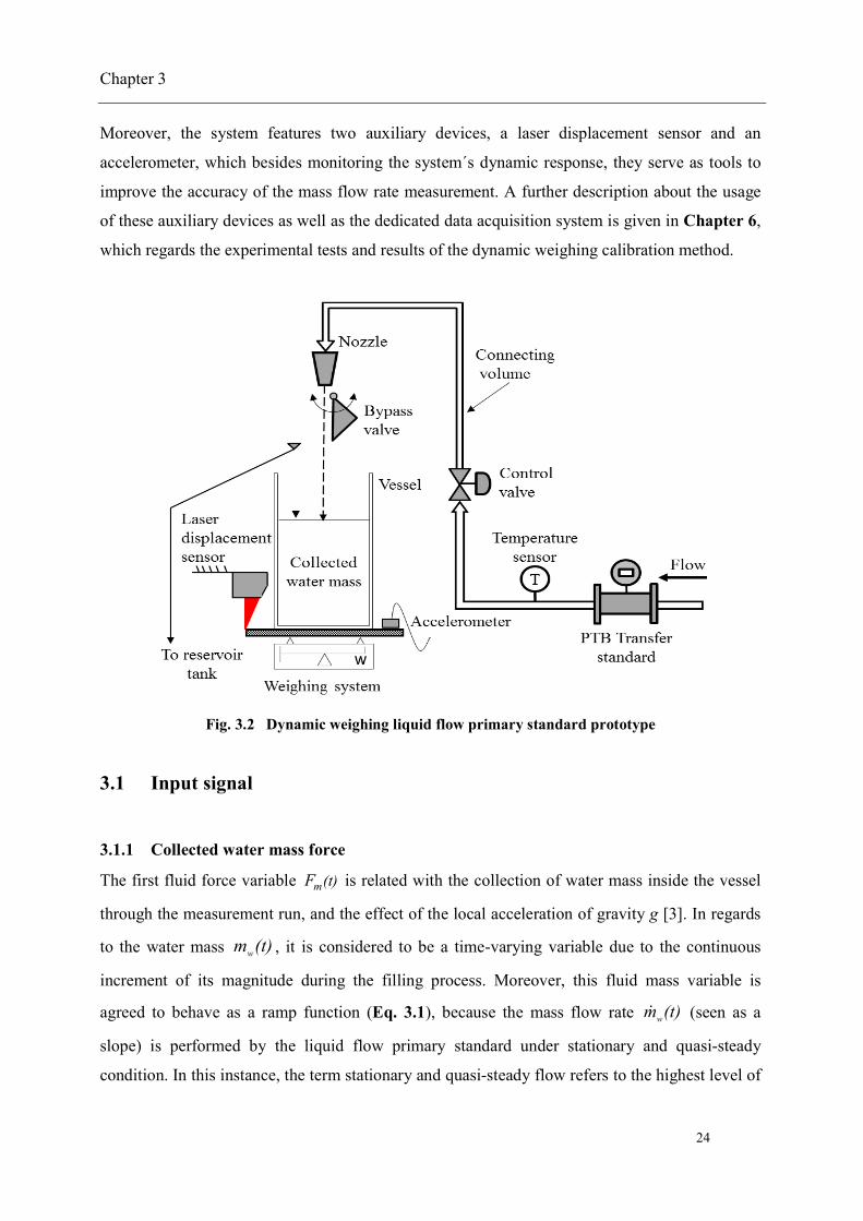
Fig. 3.2 shows the dynamic weighing liquid flow standard prototype that will be used in this
investigation, with the aim to analyze the key variables involved in this measurement process
and to realize the level of accuracy that can be achieved by using the proposed calibration
method. Such a prototype comprises an air temperature, relative humidity, and absolute pressure
sensors that serve to calculate the air density, and subsequently to correct the mass reading from
air buoyancy effects. Additionally, a nozzle and a bypass valve (with no fast actuation) are used
to discharge the water mass and drive the fluid to either, a 10-L collection vessel or back to a
reservoir tank. In terms of fluid mass transfer, the prototype features a 25-mm pipeline, which
connects a flowmeter with direct traceability to the PTB primary flow standard to the weighing
system. The goal of the flowmeter (transfer standard) is to provide a reference of how the mass
flow rate is slightly fluctuating, within its claimed measurement uncertainty, and thus comparing
its results with the given by the prototype system for validation purposes (full description in
Chapter 6). In this case, the weighing system employed is a 30-kg electromagnetic force
compensation balance (section 3.2), which holds the collection vessel, and it features a
resolution of 0,1g, with a characterized linearity of ±0,4g, and a repeatability ±0,1g.
In relation to the process conditions, such a prototype uses the PTB primary standard’s pumping
system, which ensures a stationary and quasi-steady mass flow rate as well as fluid temperature.
In addition to these control provisions, an electro-pneumatic control valve is installed upstream
the collection vessel, in order to finely adjust the flow within a range from 3 kg/min to 8 kg/min.
Chapter 3
24
Moreover, the system features two auxiliary devices, a laser displacement sensor and an
accelerometer, which besides monitoring the system´s dynamic response, they serve as tools to
improve the accuracy of the mass flow rate measurement. A further description about the usage
of these auxiliary devices as well as the dedicated data acquisition system is given in Chapter 6,
which regards the experimental tests and results of the dynamic weighing calibration method.
Fig. 3.2 Dynamic weighing liquid flow primary standard prototype
3.1 Input signal
3.1.1 Collected water mass force
The first fluid force variable m(t)F is related with the collection of water mass inside the vessel
through the measurement run, and the effect of the local acceleration of gravity g [3]. In regards
to the water mass wm (t) , it is considered to be a time-varying variable due to the continuous
increment of its magnitude during the filling process. Moreover, this fluid mass variable is
agreed to behave as a ramp function (Eq. 3.1), because the mass flow rate wm (t) (seen as a
slope) is performed by the liquid flow primary standard under stationary and quasi-steady
condition. In this instance, the term stationary and quasi-steady flow refers to the highest level of
Chapter 3
25
stability that a primary standard can achieve. Therefore, in practical terms and for the purpose of
mathematical simplification, the mass flow rate can be assumed to be a constant variable
wm (t) const in the measurement process.
m0
t
w
w 0
F (t) = m (t) g dt
m g t - t
(3.1)
In Eq. 3.1, the lower and upper limits of the integral correspond to the initial and current time of
the filling process, respectively.
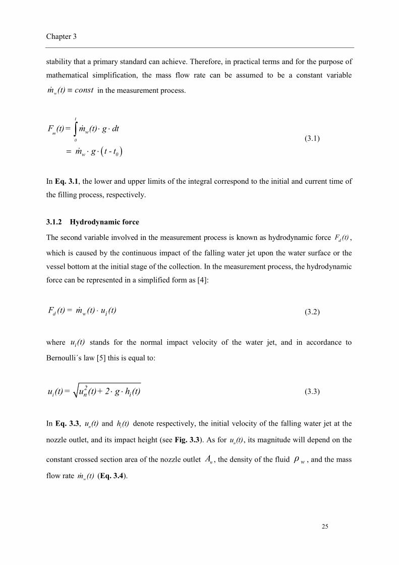
3.1.2 Hydrodynamic force
The second variable involved in the measurement process is known as hydrodynamic force dF (t) ,
which is caused by the continuous impact of the falling water jet upon the water surface or the
vessel bottom at the initial stage of the collection. In the measurement process, the hydrodynamic
force can be represented in a simplified form as [4]:
d w iF (t) = m (t) u (t) (3.2)
where iu (t) stands for the normal impact velocity of the water jet, and in accordance to
Bernoulli´s law [5] this is equal to:
i2n iu (t) = u (t)+ 2 g h (t) (3.3)
In Eq. 3.3, nu (t) and ih (t) denote respectively, the initial velocity of the falling water jet at the
nozzle outlet, and its impact height (see Fig. 3.3). As for nu (t), its magnitude will depend on the
constant crossed section area of the nozzle outlet nA , the density of the fluid wρ , and the mass
flow rate wm (t) (Eq. 3.4).

Chapter 3
26
wn
nw
m (t)u (t) =ρ A
(3.4)
The time-varying water jet impact height ih (t) can be depicted in a simplified form (Eq. 3.5) as
the difference between initial impact height ih (0) , and the continuously increasing height of the
water surface wh (t) . Thus,
i i wh (t) = h (0) - h (t) (3.5)
On the other hand, wh (t) is described by Eq. 3.6 as a related function of the current collected
water mass, the cross section area of the vessel vA , and the fluid density wρ . Hence,
0
w
ww v
t
m (t) dth (t)
ρ A
(3.6)
Therefore:
0
w
i iw v
t
m (t) dt
h (t) = h (0) -ρ A
(3.7)
Finally, after substituting Eq. 3.3, Eq. 3.4 and Eq. 3.7 into Eq. 3.2, it is found that the
hydrodynamic force is a dependent function of the mass flow rate, the fluid density, the local
acceleration of gravity as well as the dimensions and geometry of the nozzle outlet, the collection
vessel, and the constant initial water impact height (Eq. 3.8).
20( )
1 / 2
d
t
ww
w iw n w v
m (t) dtm (t) + 2 g h (0) -ρ A ρ A
tF (t)= m
(3.8)

Chapter 3
27
3.1.3 Buoyancy force
So far, the forces recalled are related to the same direction given by the gravitational force.
Nevertheless, there is still one process variable called Buoyancy force bF (t) , which also acts
upon the collected water volume but in upward direction as shown in Fig. 3.3. This force is
caused by the lifting effect (or floating effect) the air has upon the water mass, it is agreed to be
equal to the product of the increasing displaced volume by the water wV (t) , the local acceleration
of gravity g, and the air density Aρ . Then, according to Eq. 3.9, the buoyancy force [6] is
expressed as:
b w A=F (t) V (t) ρ g (3.9)
Alternatively, Eq. 3.9 can be expressed in terms of the liquid density and the mass flow rate in
order to yield:
0
tA
wb wF (t) = g m (t) dt
(3.10)
3.1.4 Total fluid force and its block diagram representation
As seen in Fig. 3.3, the liquid flow primary standard cannot longer be treated as a static system
where the collected mass is totalized; but instead, as a dynamic system driven by the summed
fluid forces of the increasing collected mass force, the hydrodynamic force caused by the water
jet impact, and the upward-oriented force of buoyancy (Eq. 3.10). Hence, the total fluid force
TF (t) acting upon the system is:
T m d b= + -F (t) F (t) F (t) F (t) (3.11)
The second and third terms of Eq. 3.11 correspond to the hydrodynamic and buoyancy force,
which are considered in this measurement process as unwanted variables. In other words, these
are the variables that have to be minimized in their magnitude by the dynamic weighing liquid
flow standard, in order to estimate with a reasonable accuracy the real mass flow rate wm (t) .

Chapter 3
28
The following Fig. 3.3 summarizes in a free body diagram and a block diagram, the graphical
representation of all considered forces and parameters involved in the measurement process.
Note that the block diagram representation of fluid forces resembles a feedforward loop, wherein
all input elements are primarily dependent of the command input, mass flow rate.
Fig. 3.3 Block diagram of the total fluid force representing the input signal of the
1-Degree-of-freedom weighing system [7]
3.2 The weighing system and its numerical representationIn general, it is understood that a balance is designed only to reproduce the unit of mass. In
principle this statement is correct, based on the fact that the weighing system manufacturers
provide an internal scale factor to convert the gravitational force exerted by a weighing object
into mass [8]. However, during the dynamic process of fluid mass collection, the utilization of
such a scale factor is not longer applicable, since the weighing system is unable to distinguish

Chapter 3
29
between the acting force attributed to the collected water mass (desired magnitude), and the
buoyancy, fluid motion and reacting system response forces [9]. Therefore, after this brief
explanation, it is understood that a weighing system is indeed a force measuring device, which
has to be re-characterized, in order to deliver a magnitude in Newtons.
For this research work, an Electromagnetic Force Compensation balance (EFC) is in use, and in
which its operational principle consists in inducing an electromagnetic force that can compensate
and equal the acting force exerted upon its weighing platform [10]. As illustrated in Fig. 3.4, the
EFC balance features an electric circuit comprising an inductive positioning sensor as well as an
oscillator and resistors R to provide a certain constant voltage V [11]. When the filling process
takes place, the fluid force causes the parallel levers to deflect or to move from its equilibrium
position. As this happens, the high-resolution inductive positioning sensor registers the current
z-axis beam location, and hence it generates a potential difference v .
Fig. 3.4 Working principle of an Electromagnetic Force Compensation (EFC) cell used as a
weighing system [11]

Chapter 3
30
Then, the potential difference magnitude is increased by a power amplifier, which delivers an
amount of current I to the coil (inserted into a permanent magnet), in order to immediately return
the beam into its zero position by changing the force of the electromagnetic field. Thereafter, an
A/D digital voltmeter acquires the voltage output signal vout , which is then filtered out by an
internal signal processing algorithm, scaled as a mass unit, and displayed.
Now, the main task in this section is to have a numerical representation of the recalled system,
which will allow a better understanding of why and how the balance responds in a certain way to
the given fluid-mechanical process conditions, and to identify the magnitude of some sources of
measurement noise. On the other hand, this model-based approach can be only valid if the
theoretical basis of the process (input, system, process model, and measurand as illustrated in
Fig. 3.1) shows a satisfactory level of agreement with the real measurement process, as
demonstrated in Chapter 5 and Chapter 6.
The proposed numerical model of the weighing system is based on Newton´s third law [12], and
it is restricted to a 1-Degree-of-Freedom (1-DoF), which is the normal axis of weighing (z axis).
Such a law states that the acting fluid forces involved in the process (Eq. 3.11), will generate an
equal but opposite response to the mechanical forces Mech(t)F exerted by the weighing system´s
elastic elements and its mass (Eq. 3.12). In other words, Eq. 3.12 says that the system struggles
at all times for an equilibrium position, due to the continuous alternation of upward and
downward forces in the process.
T Mech (t)F (t)= F (3.12)
In this instance, the balance will be represented as a system with a time-varying increasing mass,
and by two analogous elements, a damper and a spring, which simulate in a general basis the
sensing element of the balance (cell).
3.2.1 Spring force
As mentioned, one of the elastic elements employed to simulate the balance is defined by a
spring, in which its reacting force denoted by BalF (t) is equal to the product of the characterized
Chapter 3
31
balance stiffness coefficient Balk , and the displacement z undergone by the balance along the
measurement run (Eq. 3.13). This element can be also seen as the component dealing with the
storage of potential energy in the balance [13].
Bal Bal=F (t) k z (3.13)
3.2.2 Inertial force and system total mass
The second element of the system deals with its mass, and it is agreed to be equal to the
summation of: the collection vessel mass ( vm ), the weighing platform mass ( pm ), the initial
amount of water mass ( wm (0) ), and the time-varying collected water mass ( wm (t) ). As a
remark, the mass element constitutes the main mechanism of kinetic energy storage in the
balance [14], and as described by Eq. 3.14, it will turn out to be larger in magnitude as the filling
process goes on (Fig. 3.5).
T p w wvm (t) = m + m + m (0)+ m (t) (3.14)
where Tm (t) constitutes the total mass held by the balance elastic elements.
When a dynamic weighing liquid flow measurement is taking place, the continuous alternation of
acting fluid forces and reacting mechanical forces causes the system´s total mass Tm (t) to
accelerate in an oscillatory form z . Therefore, the result of this dynamic condition is an inertial
force InertialF (t) exerted upon the system, and it is described by Eq. 3.15 [15].
TInertial =F (t) m (t) z (3.15)
Here, it is important to underline, that such an inertial force is present in great part due to the
hydrodynamic force, which causes the balance to move. If the hydrodynamic force were not
present, the acceleration component in Eq. 3.15 will be zero, so that no inertial force would take
part in the process. In other words, the system would be considered as static. Furthermore, in the

Chapter 3
32
measurement process, the inertial force is subjected to decrease as the hydrodynamic force
diminishes.
3.2.3 Damping force
The third element of the weighing system model is related with the inherent characteristic of a
system to dampen (or to reduce) the oscillatory force amplitude. Or in other words, it is the
element responsible for the gradual dissipation of energy from the system [13]. In this case, the
damping force cF (t) can be determined as a product of the system z-axis velocity during a
measurement run, and the corresponding damping coefficient of the system Balc (t) (Eq. 3.16).
Subsequently, the system´s damping coefficient shown in Eq. 3.17 is agreed to be a function
dependent of the critical damping fraction (Eq. 3.18), the current system´s natural angular
frequency n (t) (Eq. 3.19), and its total mass Tm (t) [13].
Balc =F (t) c (t) z (3.16)
Bal T n= 2c (t) m (t) (t) (3.17)
1 22
d
n
1 -(t)
(3.18)
Baln
T
km (t)
(t) = (3.19)
As Eq. 3.18 and Eq. 3.19 suggest, the system damping coefficient can be alternatively expressed
in terms of the characterized spring coefficient Balk (t) , its mass Tm (t) , and the damped angular
frequency of the balance d , which is obtained (or characterized) as a function of the system
total mass Tm (t) via experimentation, then d T( m (t)) (see Chapter 5). Hence,

Chapter 3
33
BalBal T
T
1 22
d T
Bal
T
( m (t))= 2 1k
m (t)
km (t)
c (t) m (t)-
(3.20)
And after some algebraic simplifications in Eq. 3.20, the damping coefficient takes the following
form:
2 2Bal
1 2
Bal T d T T= 2 k m (t) ( m (t)) m (t)c (t) - (3.21)
3.2.4 1-Degree-of-Freedom motion equation of the weighing system
Now, at this point, the number of reacting mechanical forces of the weighing system Mech(t)F
(right side of Eq. 3.12) can be represented as the summation of:
Intertial c BalMechF (t) F (t)+ F (t)+ F (t) (3.22)
Then, Eq. 3.22 can be substituted into the into the Newton’s third law equation (Eq. 3.12), in
order to yield the system´s 1-Degree of Freedom motion equation shown in Eq. 3.23.
m d b Intertial c Bal+ -F (t) F (t) F (t) F (t) + F (t)+ F (t)= (3.23)
Likewise, the recalled system´s 1-Degree of Freedom (1-DoF) motion equation can be written in
an extended form (Eq. 3.24), with the aim to see how the motion characteristics of the balance
( z , z , and z ), the acting fluid forces, its elastic properties, its mass, and its damped angular
frequency are related into a single mathematical expression.
Tm d b Bal Bal+ -F (t) F (t) F (t) m (t) z + c (t) z + k z= (3.24)
or
2 2T Bal T d T T Balm d b
1 2+ - 2 k m (t) ( m (t)) m (t) kF (t) F (t) F (t) m (t) z + z + z-=
(3.25)

Chapter 3
34
The sketch shown in Fig. 3.5 illustrates the meaning of Eq. 3.25, stating that the balance can be
treated as a dynamic fluid-mechanical system. This analogous system comprises a collection
vessel of mass vm , enclosing a time-varying water column of mass wm (t) , in addition to a
possible amount of collected water before the measurement run wm (0) , and it is being supported
by a platform of mass pm . Such a platform is mounted on two parallel elastic elements of
stiffness coefficient Balk , and damping coefficient Balc (t) , respectively. The upper end of the
water column is agreed to be limited by a free surface at a constant atmospheric pressure, and the
effect of the local acceleration of gravity g. Additionally, the fluid and mechanical forces in this
measurement process are limited to take place along the weighing axis, therefore, the system is
subjected to have 1-DoF. In relation to its source of motion, this is assumed to come from the
command input, mass flow [16].
Fig. 3.5 Free body diagram describing the water mass and elastic elements of the system as well as
the fluid (acting) and mechanical (reacting) forces involved in the process
Alternatively, the weighing system can be also represented in Fig. 3.6 as a block diagram, with
the purpose to graphically describe the motion equation shown in Eq. 3.25. According to the
block diagram, the input signal is the total fluid force TF (t) , and it acts upon the weighing
system. In practice, there are some additional fluid forces acting upon the weighing system, such
as the vortex axial force inside the collection vessel as well as the water wave oscillatory forces

Chapter 3
35
(denoted by qF (t) ). These forces, which despite not being treated in the current analysis, they
have to be mentioned and depicted in Fig. 3.6, as a reminder that they must be investigated and
included in a future model. From the numerical analysis perspective (Chapter 5), the effect of
qF (t) upon the measurand will be overlooked, because none descriptive equation has been
derived, and added into the input signal subsystem. On the other hand, the results of
experimental tests (Chapter 6) will be limited to state that the error in calculating the measurand
is in part, due to the lack of information to quantify qF (t) . Hence, qF (t) will be assumed in the
experimental analysis as a process noise variable.
As a result of such a fluid impact force, the current system with mass Tm (t) , brakes its static
condition, and accelerates with a certain magnitude z . Then, the acceleration is time-integrated
in order to describe the system´s motion in terms of velocity z and displacement z . In this
instance, the system velocity is related with the damping coefficient of the balance sensing
element, in order to yield the so called reacting damping force cF (t) . Whereas, the product of the
system displacement, and its stiffness coefficient will be equal to the reacting balance force
response BalF (t) . The behavior of these reacting forces is seen in the block diagram as a feedback
response.

Chapter 3
36
Fig. 3.6 Block diagram representation of the balance 1-DoF motion equation (Eq. 3.25)
The outcome (or actuating signal) of this acting fluid and reacting mechanical force interaction is
denoted by the system as an inertial force IntertialF (t) , which as previously mentioned is considered
to be a source of measurement noise. The term measurement noise is used in text to underline
that such an unwanted variable is a product of the measuring device (balance) dynamic response,
and not a physical process condition.
By looking at the block diagram (Fig. 3.6), it can be also observed, that in the following times t
of the measurement process, the system acceleration z will undergo a decrement. This is
because the system mass Tm (t) gets significantly larger in comparison to the magnitude of the
inertial force IntertialF (t) . Moreover, the weighing system will inherently decrease its oscillatory
velocity and displacement, due to the balance deceleration as well as the gradual dissipation of
system energy, seen as a damping force.

Chapter 3
37
In this case, BalF (t) is representing the balance force response (output signal) because it is the
variable that summarizes in its magnitude: the acting fluid forces (input), the damping force
effect of balance sensing element, and the unwanted inertial force the system is subjected during
a dynamic process.
3.2.5 Technical considerations in regards to the modeling of the weighing system
The numerical model considered in this chapter is an analogous representation of the weighing
system, wherein its dynamic response is simulated by coupling these basic mechanical elements,
known as: damper, spring, and masses. One must be aware that during the characterization of the
weighing system, the obtained elastic properties ( Balk and Balc (t) ) and the mass magnitude used
for the numerical model, might slightly differ from the real system. This is due to the fact, that
even high-accurate weighing systems are not absolutely linear, but quasi-linear in their
response [13]. Furthermore, the numerical model is described as a 1 DoF system, in which its
motion is restricted to the normal axis of the balance z (weighing axis). However, in the reality,
the weighing system responds in a multi-axis direction (angular and translational motion), so that
a set of partial differential motion equations (including the feedback positioning control loop of
the balance) would get closer to the real system response. The multi-axis system modeling is a
concept that should be kept in mind, in order to achieve a more thorough analysis of the system
and its measurement accuracy. Nonetheless, as demonstrated in Chapter 5 and Chapter 6, the
numerical and experimental results of a 1-DoF approach turned out to be accurate enough,
meaning that the most relevant system parameters and their magnitudes are taking place at the
weighing axis.
The following remarks describe some system´s aspects that must be taken into account, in order
to avoid some misinterpretation of data when the numerical model and the real process are
compared.
The characterization of the spring coefficient Balk cannot be perfect, because the real system
may present slight non-linear force-displacement characteristics and even some hysteresis [17]
in its response. The consequence of this mechanical condition in the numerical model is a
balance force response, that might differ at some degree from the real response,

Chapter 3
38
In mechanical terms, the magnitude of the characterized system mass Tm (t) is not absolute,
because in reality, there are some additional small balance components (i.e. bolts, nuts,
levers, etc), which cannot be taken apart and weighed, and therefore are disregarded. As a
consequence, the effect of overlooking this mass will generate a slight difference in the
inertial force magnitude, in comparison with the real system when looking at its related
variable, the acceleration z ,
The characterized damping coefficient Balc (t) used in the numerical model is not exact but
approximately equal to the real system magnitude, because the natural angular frequency is a
dependent function of two other characterized system elements, Balk and Tm (t) (Eq. 3.19).
Furthermore, another reason that makes slightly different the numerical model from its
counterpart is, that the damping force is not merely produced by Balk and Tm (t) , but also by
the some small friction between balance components [13].
3.2.6 General representation of the weighing system internal filter and the discrete time
representation of its output signal
Most of commercial weighing systems used in the industry feature an internal filter, which is
responsible for minimizing the unwanted amplitude of the balance oscillatory force response, or
the inertial force as it has been discussed in the previous section. Such a type of filter can be
described in a general basis as a first-order low pass filter [18], which its aim is to allow passing
any oscillatory force response that is below to an established cutoff frequency (pass band). And
conversely, the low pass filter will eventually attenuate the amplitude of those oscillatory forces,
which are larger than the cutoff frequency (stop band).
Fig. 3.7 summarizes the low pass filter concept by presenting it in a Bode plot, in which the pass
band comprises any spectrum within a frequency ( d d 2πf ω ) lower than the cutoff frequency,
LPFf . On the other hand, as soon as the system oscillatory force equals the cutoff frequency, this
will start undergoing an attenuation in the order of -3 dB. Furthermore, if the system frequency
response is larger than the cutoff frequency, the amplitude will be reduced at a rate of 20 dB per
decade [19].

Chapter 3
39
In the practice, the internal filter of an industrial weighing system is more complex than a first-
order low pass filter. Nevertheless, due to the lack of information from the balance
manufacturers in regards to their established filter algorithms, it is in this case feasible to proceed
with a basis algorithm, which can yield a general but valid representation of what a pass/stop
frequency internal filter does.
Fig. 3.7 Bode plot representing the internal low pass filter used in the numerical model
According to Eq. 3.26, the first-order low pass filter can be simply expressed as the ratio of the
filtered output signal BalLPF dF (f ) to the input signal BalF (t) , which is equal to the level of
attenuation that the balance output signal will undergo after passing the filter. This magnitude is
known as gain factor LPF dG (f ) .
LPFBal
LPFBal
d
dd
G fF (f )
= ( )F (f ) (3.26)
Commonly, the gain factor of the low pass filter is expressed in complex terms (Left side of
Eq. 3.27), because its operation is based on a frequency domain [18]. However, it is possible to
obtain its magnitude and phase shift LPF t if the complex number is represented in a polar
form as shown in Eq. 3.27. Thus,

Chapter 3
40
1
1tand dLPF LPF LPF
LPF LPFd
LPF
2T T
T
ω ( m (t)) ω ( m (t))1G G t 1+ tω ωω (m ( ))1 i
ω
(3.27)
Eq. 3.27 indicates that in practical terms, it is possible to apply the first-order low pass filter
because the cutoff frequency LPFω information is mostly provided by the balance manufacturers,
and the oscillatory frequency of the system d T( m (t)) can be experimentally obtained by
characterizing the oscillatory mechanical response of the balance.
Fig. 3.8 illustrates in a block diagram, the implementation of low pass filter (Eq. 3.26 and
Eq. 3.27), depicting that the continuous-time response of the balance BalF (t) stands for the input
signal of the internal filter. On the other hand, the block diagram describes the current frequency
of the oscillatory weighing system d T( m (t)) , and the cutoff frequency LPFω as the responsible
variables for tuning the gain of the filter. Finally, BalLPFF (t) and LPF t denote respectively, the
balance response after attenuating its oscillatory magnitude and phase shift.
Fig. 3.8 First-order low pass filter in a 1-Degree-of-Freedom weighing system model
At this stage of the process, the balance response signal has been presented in terms of a
numerical model, and its output signal is agreed to be attenuated in a continuous-time form by a
low pass filter. However, for an appropriate comparison and analysis of the weighing system, it

Chapter 3
41
is still required to represent the balance output signal response in a discrete-time form, as it is
delivered by the physical system.
Such a discrete-time conversion shown in Eq. 3.28 is carried out by first defining the
continuous-time output signal, which is BalLPFF (t) . The second part of the equation comprises a
series of Dirac impulses, that acquire data only at constant time intervals along the measurement.
The impulse function for this application is described as the difference between a given time t
within the measurement, and the product of the data sampling number N and the system’s data
sampling time st . In other words, sδ(t - N t ) [18].
Bal BalLPFn sN=0
F (t )= F (t) δ(t - N t )
(3.28)
Fig. 3.9 describes the continuous-discrete time conversion in Eq. 3.28 as a block diagram, and it
illustrates the expansion of its cumulative sum in a cascade form.
Fig. 3.9 Continuous/discrete time conversion of the balance output response

Chapter 3
42
3.3 The connecting volume effect in liquid flow measurementsFor the sake of explanation, the definition of mass and volumetric flow in a closed conduit
system was presented in Chapter 2 in terms of a simplified form of the continuity equation
(Eq. 2.1). However, in practice, if such a simplified equation were intended to be used in a liquid
flow primary standard, the expected result would be a mass flow rate calculation with reduced
measurement accuracy, as it neglects the storage effect from the connecting volume (pipeline
between the flowmeter under calibration and the weighing system). In other words, this effect
indicates that in a real system, the eventual temperature changes of the fluid and the pipeline
material will cause the fluid mass inside the connecting volume (CV) to change during the
measuring time, and as a consequence, the mass flow circulating through the installed flowmeter
will differ in some degree from the mass flow being discharged into the collection vessel and
measured by the liquid flow primary standard (Fig. 3.10).
In this instance, the general continuity equation shown in Eq. 3.29 is the basis equation
employed in flow calibration facilities to quantify the connecting volume effect in the
measurement [20]. The following equations and text below describe the background of this
equation. As written in Eq. 3.29, the continuity equation establishes that the summation of the
rate of change of mass inside a selected connecting volume CVV (first term), plus the mass flow
rate passing through an arbitrary area of the connecting volume CVA (second term) has to be
equal to zero, in order to comply with the law of mass conservation [20].
w_CV w_CV
CV CVV A
d ρ dV + ρ u( t ) dA= 0dt
(3.29)
Here, w_CVρ and u( t ) denote respectively the water density in the connecting volume (CV), and
the mean velocity of the fluid at an arbitrary region across the CV.
Now, for the purpose of applying the general continuity equation, Eq. 3.29 has to be derived in
terms of the boundary conditions of the liquid flow primary standard. First, since there is no
mass flow passing through the walls of the pipeline, it is inferred that the product u( t ) dA of the
integral for this portion of surface is equal to zero. On the other hand, the mass is indeed flowing

Chapter 3
43
in a normal direction to the cross section area of the flowmeterMeterA (inlet section) as well as the
cross section area of the nozzle outletnA (outlet section). Therefore, in accordance to the given
statements, Eq. 3.29 can be written for this specific case as [21]:
w_CV w_Meter w_nMeter
nMeterCV
IN OUT
nV A A
+ +d ρ dV - ρ u ( t ) dA ρ u ( t ) dA = 0dt
(3.30)
In Eq. 3.30, w_Meterρ and w_nρ stand for the water density at the flowmeter and the nozzle outlet
location. Furthermore, the termsMeteru ( t ) and nu ( t ) represent the mean normal velocity of the
fluid at the flowmeter and nozzle outlet location. Moreover, the second and third term of
Eq. 3.30 correspond respectively to the inlet and outlet mass flow of the control volume. Note
that the minus sign at the inlet surface term is given, because the flow direction is opposite to the
pressure force direction exerted by the water enclosed in the connecting volume [22].
Fig. 3.10 The connecting volume of a liquid flow primary standard

Chapter 3
44
Moreover, in accordance to the law of mass conservation, it can be stated that the mass outflow
of the control volume (third term of Eq. 3.30) is equal to the mass flow rate delivered to the
dynamic weighing liquid flow standard ˆnwm ( t ) , as illustrated in Fig. 3.10. Likewise, the same
statement applies for the mass flow rate passing through the inlet section of the CV (second term
of Eq. 3.30), which in practical terms turns out to be equal to the mass flow rate measured by the
flowmeter Meter nm ( t ) . Thus,
ˆw_CV Meter
CV
n w nV
( t ) ( t )d
ρ dV m +mdt
- = 0 (3.31)
In a more thorough description, Eq. 3.32 points out the two physical effects that cause the fluid
mass to change in the CV (first term of Eq. 3.31). One is originated by the pipeline volume
change due to the thermal expansion or contraction of its material in a certain time, and the
second effect is regarded to the fluid density variations inside the CV with respect to time.
w_CV CV
w_CV
CV
w_CVCVCVw_CV
V
V
d ρ Vd ρ dV =dtdt
d ρd= ρ Vdt dt
(3.32)
Then, in order to find out the practical-oriented solution to this analysis, the rate of mass change
depicted in Eq. 3.31 has to be represented as the limit of the nominal change of water mass
within a time interval Δt that approaches to zero. Hence,
0 0lim lim
w_CV w_CVt t
CV
CV w_CVCV
V
dρ dV ρ V
dt t t
V ρ=
(3.33)
where the time interval is defined as:
Δ n n-1 st = t - t t (3.34)

Chapter 3
45
Therefore, due to a small temperature changes in the CV, and the thermal expansion properties
of the fluid and pipeline material, the nominal change of fluid density and CV volume are
assumed to be [23]:
Δw_CV w_CV w_CVw=ρ - ρ β (3.35)
ΔCV CV CV CV=V V 3 α (3.36)
As for the equations above, wβ denotes the volumetric thermal expansion coefficient of water
( -6207 10 / K ), and CVα is the linear expansion coefficient for the connecting pipe ( -617,3 10 / K ) [24].
Meanwhile, the variables Δ w_CV and Δ CV described in Eq. 3.35 and Eq. 3.36, correspond to
the undergone temperature difference of water (Eq. 3.37) and pipeline material (Eq. 3.38)
between the time step n-1t and nt . Hence,
Δ n n-1w_CV w_CV w_CVt t (3.37)
Δ n n-1CV CV CVt t (3.38)
Thus, after substituting Eq. 3.34, Eq. 3.35 and Eq. 3.36 into Eq. 3.33, the rate of change of mass
in the CV (connecting volume effect) can be determined by the following expression [23]:
Δ Δ
Δ Δ
CV CV CV CV w_CV w w_CVw_CV w_CVV CV
CV CV CV w w_CVw_CV s
d ρ dV ρ 3 V α V ρ β tdt
ρ V 3 α β t
(3.39)
Finally, Eq. 3.39 can be substituted into Eq. 3.31, in order to yield a practical form of the
continuity equation (Eq. 3.40), which helps to correct the measurement error caused by the
storage effect of the connecting volume, and thus it allows comparing both measurement
approaches.

Chapter 3
46
Δ Δˆ CV CV CV w w_CVw_CVMeterw n n
s
ρ V 3 α βm ( t )= m ( t ) -
t
(3.40)
3.3.1 Accuracy considerations in relation to the connecting volume effect in dynamic
weighing liquid flow measurements
The significance of the discussed connecting volume effect upon the flow measurement accuracy
can depend not only on the fluid and pipeline material temperature, but also on the type of
primary standard in use. The following calculation examples shown in this section are made with
the purpose to illustrate the impact of the connecting volume effect in the measurand, when this
parameter is neglected either in a static weighing or in a dynamic weighing mass flow
measurement.
The first calculation is based on a measurement run performed by the liquid flow primary
standard, assuming this operates in a static-weighing mode at an average mass flow rate wm of
8 kg/min, with a collection time of 60s in a 10-L vessel. In this instance, the fluid and connecting
volume temperature variations during the collection time are respectively 50 mK and 200 mK,
based on data observations from a liquid flow primary standard. Additionally, the water density
is agreed to be 998,2 kg/m³ at 20°C [25], and with a nominal connecting volume of 0,7 L. Thus,
in accordance to Eq. 3.39, the magnitude of the connecting volume effect in a static-weighing
mode (for this example) is:
CV
-6 -6
w_CVV
Static
-8
kg 1 1998,2 0,0007m 3 17,3 10 0,2K - 207 10 0,05Km K Kρ dV
1min60s 60 skg= 2,096 10
min
³³
(3.41)
Or in terms of its relative uncertainty:
CV
w_CVV
StaticCV Static
w-7
ρ dV
U = 100%m
= 2,62×10 %
(3.42)
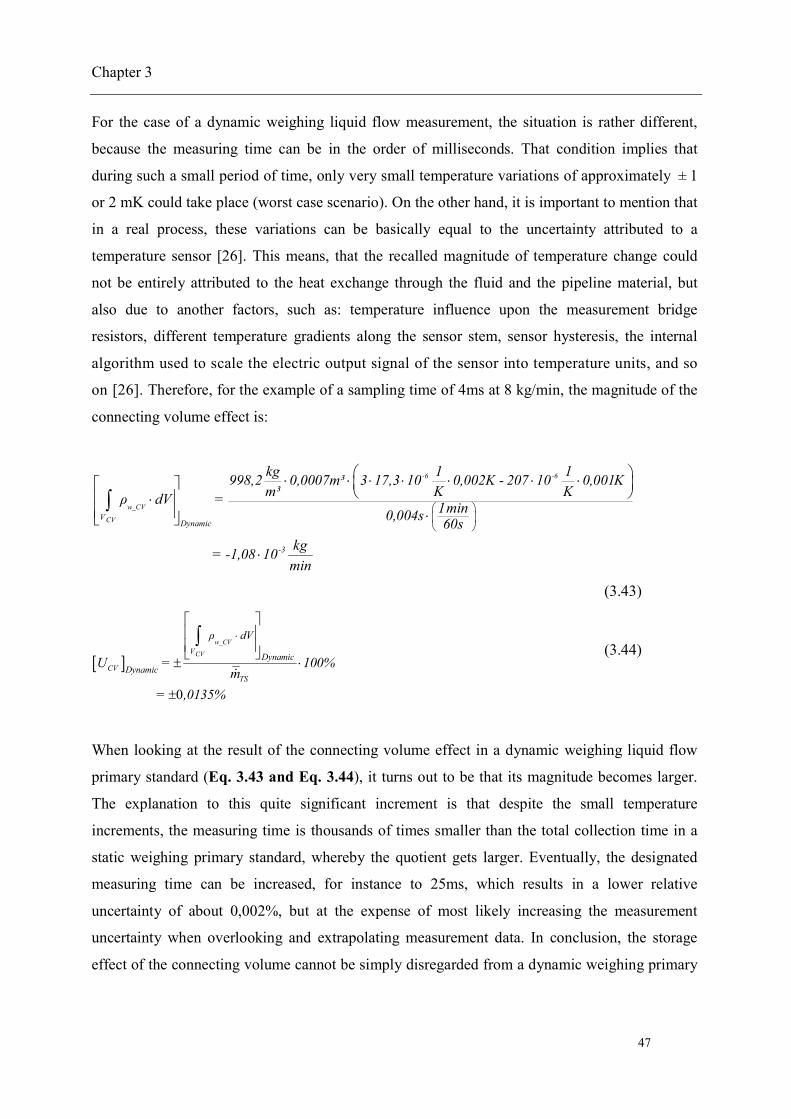
Chapter 3
47
For the case of a dynamic weighing liquid flow measurement, the situation is rather different,
because the measuring time can be in the order of milliseconds. That condition implies that
during such a small period of time, only very small temperature variations of approximately ± 1
or 2 mK could take place (worst case scenario). On the other hand, it is important to mention that
in a real process, these variations can be basically equal to the uncertainty attributed to a
temperature sensor [26]. This means, that the recalled magnitude of temperature change could
not be entirely attributed to the heat exchange through the fluid and the pipeline material, but
also due to another factors, such as: temperature influence upon the measurement bridge
resistors, different temperature gradients along the sensor stem, sensor hysteresis, the internal
algorithm used to scale the electric output signal of the sensor into temperature units, and so
on [26]. Therefore, for the example of a sampling time of 4ms at 8 kg/min, the magnitude of the
connecting volume effect is:
-6 -6
w_CV
CVVDynamic
-3
kg 1 1998,2 0,0007m³ 3 17,3 10 0,002K - 207 10 0,001Km³ K Kρ dV = 1min0,004s 60s
kg= -1,08 10min
(3.43)
0
w_CV
CVV
CVTS
DynamicDynamic
ρ dV
U = 100%m
= ,0135%
(3.44)
When looking at the result of the connecting volume effect in a dynamic weighing liquid flow
primary standard (Eq. 3.43 and Eq. 3.44), it turns out to be that its magnitude becomes larger.
The explanation to this quite significant increment is that despite the small temperature
increments, the measuring time is thousands of times smaller than the total collection time in a
static weighing primary standard, whereby the quotient gets larger. Eventually, the designated
measuring time can be increased, for instance to 25ms, which results in a lower relative
uncertainty of about 0,002%, but at the expense of most likely increasing the measurement
uncertainty when overlooking and extrapolating measurement data. In conclusion, the storage
effect of the connecting volume cannot be simply disregarded from a dynamic weighing primary

Chapter 3
48
standard. As suggested by these examples and in the following Chapter 5 and Chapter 6, this
effect can be considered as the third main uncertainty contributor in the measurement process
after the mass flow calculation model, and the process and measurement noise (Table 3.1).
According to reference [27] the connecting volume effect stands as the fifth uncertainty
contributor for static weighing calibration systems.
Table 3.1 Main uncertainty contributors of the static [27] and dynamic weighing liquid flow
primary standards

Chapter 4
49
4. Filtering techniques for the determination and accuracy of mass
flow rate (Process model)
In this chapter, a series of filters are presented with the aim of processing the acquired data from
the weighing system output signal Bal nF (t ) , and thus, delivering an estimate of the desired
measurand, mass flow rate.
The block diagram sketched in Fig. 4.1 stands for the recalled three main subsystems of the
dynamic weighing liquid flow primary standard. In Chapter 3, a description of the command
input as well the first two subsystems (Fluid force and weighing system) were presented. Now,
Chapter 4 will address with the third subsystem known as Process model, which has to be
expressed in a discrete-time form nt , due to the time constant of the balance output signal, and
data acquisition system involved in the real measurement process.
As seen in Fig. 4.1, the process model subsystem is divided into two subsystems called
respectively: Hydrodynamic force filter and Measurement noise filter. The Hydrodynamic force
filter has the task to analytically quantify and eliminate (or drastically reduce) the magnitude of
the disturbing state variables from the measurement process; so the measurand ˆnHFm (t ) can be
dynamically estimated with a higher accuracy [1]. As mentioned in Chapter 3, such disturbing
process variables are described as: the hydrodynamic force ( )d nF t driven by the impacting
water jet, and in a minor degree, the upward air buoyancy force ( )b nF t that causes an apparent
loss of collected mass force [2]. The latter occurs either under dynamic or static measurement
conditions.
The second subsystem known as measurement noise filter comprises a signal filter algorithm,
which deals with the identification and attenuation of the measurement noise [3], and it is
originated in great part by the reacting inertial force ( )Inertial nF t of the weighing system. The
task of this filter is to make the estimate measurements ˆnwm (t ) more precise [4], and to re-
enhance their accuracy.

Chapter 4
50
Fig. 4.1 General block diagram representation of the process model, its two subsystems, and the
treatment of the measurement data to estimate the mass flow rate
As shown in Fig. 4.1, e denotes the estimated error, nwm (t ) is the true measurand value, f(m)
stands for the probability distribution of m [5], and ˆnBalm (t ) , which is the estimate value of
mass flow rate given by the direct response of the balance (Eq. 4.1). As a remark, it is important
to note that ˆnBalm (t ) is indeed an estimate measurand value, but it has not been treated by the
influence of the hydrodynamic and buoyancy forces, in addition to the measurement noise
induced by the dynamic response of the weighing system.
0
0
ˆ Bal BalBal
n
nn
F (t ) F (t )g t t
m t -( )
(4.1)

Chapter 4
51
4.1 Derivation of a filter for the attenuation of the hydrodynamic force effect
upon the balance output response and determination of mass flow rateOne form to derive an algorithm that can filter out the presence of the discrete-time
hydrodynamic and buoyancy force from balance output signal, consists in analyzing the
1-degree-of-Freedom motion equation derived in Chapter 3 (Eq. 4.2), because it is the equation
that relates the recalled unwanted fluid state variables, with the response of the balance used in
the process.
n n n n n nIntertial c Bal m d b+ -F (t ) + F (t ) + F (t ) F (t ) F (t ) F (t ) (4.2)
As mentioned in Chapter 3, it is agreed that Bal nF (t ) denotes the balance response because is
indeed the variable that summarizes in its magnitude: the acting fluid forces, the damping force
effect of the balance sensing element, and the inertial force the system is subjected during the
dynamic process (Section 3.2.4). Hence, the equation of motion can be expressed as Bal nF (t ) ,
equal to the summation of all involved acting-reacting forces (Eq. 4.3)
n n n n n nBal m d b Intertial cF (t ) F (t )+ F (t ) - F (t )- F (t ) - F (t ) (4.3)
In the real measurement process, the balance is unable to measure each of the fluid force
variables independently, but their summation represented by the variable called T nF (t ) , in
addition to the mechanical reacting forces of inertia and damping, as shown in Eq. 4.4.
n n n nBal T Intertial cF (t ) F (t ) - F (t ) - F (t ) (4.4)
Now, for the sake of obtaining a practical equation for the determination of mass flow rate, it is
necessary to simplify Eq. 4.4 based on the physical fact, that the balance force response Bal nF (t ) ,
and the acting fluid forces are estimated to be equal (Eq. 4.5) [6]. The explanation for this
assumption is the following.
�������� ≜ ����� (4.5)

Chapter 4
52
Firstly, consider the Force-time graph shown in Fig. 4.2(a), wherein T nF (t ) is split into its three
components: collecting mass, hydrodynamic, and buoyancy force. On other hand, take a look to
Fig. 4.2(b), in which the path of a ramp-like response of T nF (t ) and Bal nF (t ) are basically
overlapping all along the filling process. In other words, the average slope magnitude is agreed
to be the same in both cases. However, the relatively small difference still remaining between
these two state variables T nF (t ) and Bal nF (t ) is due to the inertial force Intertial nF (t ) , damping
force ncF (t ) , in addition to the balance time response, the effect of the continuous-discrete time
conversion, and low pass filter upon the balance output signal. These signal-conditioned
unwanted state variables will be treated in the following section, regarding the measurement
noise filter and its application. Summarizing, Eq. 4.6 gathers the above statements in an
expression, describing that the balance output response can be equal to the summation of
estimated fluid force variables, denoted by a hat symbol “^”.
Fig. 4.2 Graphical representation of (a) acting fluid forces and (b) balance force response during
the filling process
Bal n m n d n b nF (t )= F (t ) F (t ) F (t ) ˆ ˆ ˆ (4.6)
After writing Eq. 4.6 as a function of mass flow rate in terms of the discrete time form nt , the
equation takes the following form:

Chapter 4
53
ˆ ˆ ˆˆ
ˆ ˆ1HF
ABal n HF n n HF n n HF n
w
An n
w
n
n
i
i
t
( ) t
+F (t )= m (t ) g t m (t ) u (t ) m (t ) g
m t g u (t )
-
(4.7)
where the subindex HF stands for the mass flow rate estimate after applying the hydrodynamic
force filter, g is the local acceleration of gravity (9,8125 m/s²), and ˆi nu (t ) is the water jet impact
velocity.
Then, after substituting the hydrodynamic force equation (Eq. 3.8) in a discrete-time form into
Eq. 4.7, such an equation becomes:
ˆ ˆˆ 1
ˆ ˆ
HF HFHF
1/ 2
n n nAnBal n n
w
2
iw n w v
n n ni
m (t ) m (t ) tF (t ) m (t ) g +2 g h (0)-ρ A ρ A
u (t ) h (t )
t
(4.8)
As a remark, it is important to underline that in Eq. 4.8, the local acceleration of gravity g is
considered as a constant, due to the fact that the changing center of gravity of the water mass
during the filling process, and the effect it has upon the g value is relatively small [7]. Now, in
order to carry on with the equation to estimate the measurand ˆHF nm (t ) , it is necessary to express
Eq. 4.8 in a form that the square root of the impact velocity can be cancelled out, and thus
making the factorization easier. Hence,
2
2
ˆ
ˆ ˆˆ
ABal n HF n n
w
1/ 2
HF n HF n nHF n
2
iw n w v
F (t ) - m (t ) g 1 - t
m (t ) m (t ) tm (t ) + 2 g h (0) -ρ A ρ A
(4.9)

Chapter 4
54
And after some algebraic steps in Eq. 4.9, it turns out to be that the hydrodynamic force filter
equation is a polynomial equation of fourth order, and it is described in the following canonical
form:
2
ˆ ˆ ˆ
ˆ
HF HF HF4 3 2A
n n nw
ABal n n HF n Bal n
w
22 2n
i n2 2w vw n
2 g t1 m (t ) m (t ) + 2 g h (0) g 1- t m (t )ρ Aρ A
...+ 2 F (t ) g 1- t m (t ) F (t )=0
- ...
-
(4.10)
As Eq. 4.10 indicates, the determination of the measurand ˆHF nm (t ) cannot be obtained by simply
substituting the variables into the equation, as that occurs in a second-order equation, wherein its two
roots (not necessarily distinct) are obtained by simply using the so called Quadratic formula [8]. One
practical way to accurately solve Eq. 4.10 consists in implementing a numerical method that can
calculate the eigenvalues (or roots) of such a polynomial equation. In this instance, Eq. 4.11
shows the characteristic time-varying matrix nE [9] of the fourth order equation, wherein its
coefficients are contained.
( ) / ( ) ( ) / ( ) ( ) / ( ) ( ) / ( )1 0 0 00 1 0 00 0 1 0
n n n n n n n n
n
b t a t c t a t d t a t e t a t
E (4.11)
where the order of these coefficients in relation to Eq. 4.10 as well as its variable is written as:
n n n n n4 3 2
n n n n np( (t )) a(t ) (t )+b(t ) (t )+c(t ) (t )+d(t ) (t )+e(t )= 0 (4.12)
In order to find out the eigenvalues of Eq. 4.10 for each time step nt , such an equation has to be
represented in an equivalent form, in which the determinant of its characteristic matrix nE minus
the dot product of the scalar values n(t ) and the identity matrix I is equal to zero, as shown in
Eq. 4.13. Likewise, this polynomial equation can be written in a factorial form, in order to
describe more clearly the eigenvalues nE .

Chapter 4
55
1 2 3 4
det( )( ) ( ) ( ) ( ) 0n n n n n n n n
nn np( (t )) (t )(t ) - (t ) (t ) - (t ) (t ) - (t ) (t ) - (t )
E I
(4.13)
In this instance, Eq. 4.13 is solved by a robust numerical method called QR algorithm [10 and
11], which is available in some technical computing software, such as MatLab®, and it allows a
fast and an effective iterative method to calculate the eigenvalues of the characteristic matrix nE .
Furthermore, it is important to note that in Eq. 4.12 and Eq. 4.13, the scalar n(t ) is
intentionally used to represent the main variable of the polynomial equation p( ) , instead of the
measurand ˆHF nm (t ) shown in Eq. 4.10. The reason is that after solving the determinant, the four
eigenvalues found 1 2 3, ,n n n(t ) (t ) (t ) and 4 n(t ) can be either equal or distinct among each
other (Eq. 4.14). In this case, only the real part of the complex number eigenvalue is taken into
account, and the selected eigenvalue is the one that gets closer to the average estimate mass flow
rate ˆnBalm (t ) yield by Eq. 4.1.
1 2 3 4ˆ
HF n n n n nm (t )= (t ) (t ) (t ) (t ) (4.14)
where the symbols “ ” and “ ” stand respectively for the logical operators “and” and “or”.
As for the experimental determination of mass flow rate ˆHF nm (t ) , this follows in principle the
same methodology used for the numerical approach. Nevertheless, in the real process, additional
considerations have to be taken into account, because the water and air temperature ( w and A )
and consequently their densities, can change during the measurement run. Hence, the water and
air density variables are agreed to be temperature-depended variables denoted as w wρ ( ) and
A Aρ ( ) .
Another consideration to make during the experimentation is that the estimate impact height
component i nh (t ) described in Eq. 4.8 can yield to some calculation errors, due to the fact that
the cross section area of the collection vessel vA can significantly vary from its nominal value at

Chapter 4
56
different locations, especially at the vessel bottom. Therefore, in order to attain a better estimate
value of the impact height, a characterization will be carried out to get an equation that can relate
the changes of the water surface level wh , with the imminent displacement of the balance
platform z when the mass increases. In other words, the impact height will be experimentally
defined as a function of the balance platform displacement denoted as ih (z) .
It is worth to mention that an impact height equation via a characterized cross section area of the
vessel vA is also possible. However, it can be a quite challenging and time-consuming task in
terms of (i.e. cylindrical vessel) [12]: mounting a length standard inside the vessel, moving the
length standard not only in a translational but also in a rotational form, so the vessel diameter can
be characterized at different lengths and locations. In addition to the above mentioned issues, the
roundness errors can be also rather significant, for the fact that most vessels are designed and
manufactured as containers. Nevertheless, if the vessel were a high-accurate rounded-shape
cylinder, the characterization of vA would result in a better approach for calculating i nh (t ) , from
the point of view of reducing the number of process variables as well as the number of
measurement uncertainty contributors.
The details of the impact height characterization procedure via balance platform displacement
are described in Chapter 6, regarding the experimental setup of the prototype used as a dynamic
weighing liquid flow primary standard.
Hence, after considering the above statements, the experimental equation for the estimation of
the water mass flow rate can be written as follows:
2
( )
( )( )
( )
( )
ˆ ˆ ˆ
ˆ
A
ww
A
w
AHF n HF n
w
ABal n n HF n Bal n
w
24 2 2 2
i n2 2w n
1 m (t )+ 2 g h (z) g 1- t m (t )+...ρ A
...+ 2 F (t ) g 1- t m (t ) F (t )=0
(4.15)
As a remark, the eigenvalue method used to iteratively solve the numerical approach is also
employed to obtain the experimental estimate collected mass and flow rate from Eq. 4.15.

Chapter 4
57
4.2 Proposed filter algorithms for an improved mass flow rate calculation
based on the identification and reduction of measurement noiseSo far, the hydrodynamic force filter (first process model subsystem) enables to represent some
physical phenomena that are implicit in the process, as well as depicting a mathematical model
that can help to separate, or at least to attenuate the unwanted process variables from the
measurand. Now, the second process model subsystem, known as Measurement noise filter is
dealing with one particular issue: The weighing system do not provide the exact desired quantity
w nm (t ) , because it introduces its own system dynamic response into the output signal HF nm (t ) ,
which adds in a major or a minor degree measurement noise nv(t ) (Eq. 4.16).
HF n w n nm (t ) =m t v t ˆ (4.16)
For the treatment of the measurement noise in the liquid flow primary standard, three different
filter algorithms are proposed, with the aim to realize, which one delivers the most precise and
accurate estimate value (Fig. 4.3). These filters are:
1) Central moving average filter [13], which aims to smooth out the trend of the measurand by
creating a plot line of connected data subset averages, defined by a certain number of
measurement data before and after the current time step nt ,
2) Least-Mean-Square adaptive filter, which adapts to the input signal by iteratively tuning its
parameters (i.e. curve-fitting), in order to deliver an estimate value with a minimized signal
error [14 and 15], and
3) Linear Kalman filter algorithm that combines all available measurement data, plus prior
knowledge of the weighing system, in order to produce an estimate measurand, wherein its
error is statistically minimized, and it does not require to store and reprocess large amounts
of previous measurement data to deliver its output [16].

Chapter 4
58
Fig. 4.3 The measurement noise filter and the three selected filters for the analysis
4.2.1 Central moving average filter
The central moving average is a type of filter that estimates the value of the measurand by
averaging several values from a number of data subsets, and thus repeats the same procedure for
the whole measuring time of the process.
The moving average is the first filter considered in this work, due to its simplicity for its
implementation, but also because of its ability to drastically decrease the amplitude of
measurement noise from the input signal HF nm (t ) , while keeping a sharp step response to
changes in the measurand [17]. As an important remark, the central moving average filter in
use is indeed a data smoothing algorithm. This means, an algorithm that can prevent a large
erroneous shifting of the estimate values by not only considering the measurement data
before the reference time tn (as it is the case of an ordinary moving average) but also the data
after tn [18]. As illustrated in Fig. 4.4, this algorithm can be also represented as a
combination of two filters. In this instance, one of the filters averages all the a priori data to
time tn to produce an estimate ˆ )+MA nm (t . This can be recalled as a forward filter. Meanwhile, the
second filter (backward filter) averages all the a posteriori data to time tn, and gets the second

Chapter 4
59
estimate ˆ )-MA nm (t . Then, by putting together these two filters, a more accurate estimate ˆ )MA nm (t
of the measurand can be achieved (Eq. 4.17), when analyzing two different trends of mass flow
rate between time tn [19].
nn
MA
MAMA MA
MA
MA
MAMA
HF HF
HF
m tm t
n+ N 2n
n i ii=n N 2 i=n+1
n+ N 2
ii=n N 2
-
-
1 1 1m t = m t m t2 N 2 N 2
1= m tN
ˆˆ
ˆ ˆ ˆ
ˆ
MAMA
(4.17)
According to Eq. 4.17, NMA denotes the number of data samples to average by the filter, and n
stands for the measurement sample to be smoothed out. Furthermore, one must be aware about
the appropriate designation of NMA, due to the fact that an excessive number of samples can
eventually produce a stiff filter output response, leading to a possible misinterpretation of the
measurand [19].
Fig. 4.4 Block diagram representing the central moving average filter algorithm [14]

Chapter 4
60
4.2.2 Least-Mean-Square adaptive filter
As the name suggests, this type of filter adapts to the performance of the input signal delivered
by the previous hydrodynamic force filter HF nm (t ) , with the aim to learn how to distinguish
between the measurement noise caused by the oscillatory motion of the balance, and the true
measurand. Then, such information is used to proceed with the removal (or high attenuation) of
the noise from its input signal, and thus, yielding an estimate of the measurand [15]. The general
concept about how this type of filter operates is graphically depicted in Fig. 4.5. Firstly, the
scheme in Fig. 4.5 refers to an input signal, wherein the true measurand value is corrupted with a
time-varying noise amplitude [20].
Secondly, making reference to Fig. 4.5, the filter incorporates in its structure a decorrelation
delay, followed by the basis Least-Mean-Square (LMS) algorithm of the adaptive filter. The
decorrelation delay is in this instance a useful statistical tool, which helps to identify the
measurand from the noisy input signal by comparing a version of the input signal HF nm (t ) with a
second version that has been delayed D intervals HF n-Dm (t ) . The decorrelation delay D is not a
number that can be given arbitrarily. On the contrary, it must be chosen so that the signal value
HF nm (t ) will not correlate either with HF n-Dm (t ) or with respect to nv t . In other words, none
similarities or repeating patterns must appear between them [21].
The basic working principle of the LMS adaptive filter algorithm exemplified in Fig. 4.5 consists
in applying an iterative approximation technique, where its outcome AF nm (t ) is given by the
summation of convoluted filter coefficients h(k) , and the decorrelated input data (Eq. 4.18).
HF
M -1
AF n n D kk=0
m t = h k m t - - ˆ ˆ (4.18)
where M denotes the number of filter coefficients, and AF nm (t ) is the estimate measurand yield
by the adaptive filter (output signal).

Chapter 4
61
The filter coefficients recalled in Eq. 4.18 have the task to approach the measurand value by
attenuating the input signal amplitude (this means, narrowing the spread of the measurement
noise), and in this manner, making the estimates more accurate along the measuring time. As a
remark, the level of accuracy and convergence of the adaptive filter depends in many cases of the
number of filter coefficients used in the algorithm [22].
In regards to the iterative part of the LMS adaptive filter, this is based on the ongoing renewal of
its coefficients h(k) , so the measurand can be better estimated after each step [23]. As depicted
in Fig. 4.5, the numerical process of updating the filter coefficients consists firstly in using the
values of the previous step filter coefficients as current values called ch (k) . Thereafter, such
current filter coefficient values are sum up with the product of the feedback error signal value
( )AF ne t , the filter step size ΔAF , and the decorrelated delay input signal value m HF n-D-km t , in
order to yield a set of updated filter coefficients, uph k (Eq. 4.19).
Δ HFup c AF AF n n-k-Dh k = h k + e t m t (4.19)

Chapter 4
62
Fig. 4.5 Block diagram of a delayed input Least-Mean-Square adaptive filter for noise removal
[20]
As observed in Eq. 4.20, Fig. 4.5, and Fig. 4.6, the feedback estimate error signal ( )AF ne t
reveals a particular feature of this filter, which unlike the adaptive filters for system
identification (see reference [24]), it seeks for the minimization of error by comparing the
difference between the estimate value ˆ ( )AF nm t , and the measurement input signal HF nm t [21].
In other words, ( )AF ne t can be referred as the estimate version of the measurement noise nv(t )ˆ ,
due to the fact that ˆ ( )AF nm t is also an estimate value of the true measurand value w nm t .
HFAF n n AF n
n
e t =m t - m t
v t
ˆ ˆˆ
ˆ (4.20)

Chapter 4
63
Fig. 4.6 Graphical explanation of the estimate error signal feedback [21]
The determination of filter step size ΔAF (Eq. 4.21) is another crucial task for the successful
implementation of the algorithm into the measurement process. Such a variable is responsible for
determining the amount of correction to be applied as the filter adapts from one iteration to the
next. In order to choose the appropriate step size, it is necessary to take into account the
following considerations [25 and 26]:
1) If the step size is too small, the time of convergence (based also on the number of filter
coefficients) can be too long, so that the estimate value might never reach an accurate enough
value,
2) If the step size is too large, that might cause the adaptive filter to diverge, and becoming
unstable.
Therefore, in order to ensure satisfactory convergence and stability in the filter, the step size ΔAF
must be within a recommended range [21]:
ΔAFAF
10 < <10 M P (4.21)

Chapter 4
64
where M is the number of filter coefficients, and AFP is the average power of the input signal
data set, and it is described as:
AF
HF
N2
AF nAF n=0
1P =N +1
m t (4.22)
Here, AFN represents the number of input signal data.
As a remark, it is recommended to start with small step sizes, so that the estimate values of the
filter can be more reliable in terms of its accuracy level, but at the expense of the taking some
additional time to adapt the filter into the measurand [23].
The delayed input signal LMS adaptive filter algorithm is not the only method employed by
adaptive filtering theory to remove noise. For instance, the Normalized Least-Mean-Square
adaptive filter (NLMS) can converge more quickly than the LMS due to its time-varying step
size that minimizes the instantaneous estimate error [23 and 27]. Moreover, the Recursive Least-
Square (RLS) [28] exhibits an even faster convergence speed than the LMS or NLMS, because
its time-varying estimate error uses a statistical factor, the Kalman filter will be described, with
the aim to analyze the effectiveness of such recursive filtering techniques in this particular
process [29]. Furthermore, despite the recalled enhanced performance of the NLMS and RLS in
relation to LMS, the LMS has three significant characteristics that makes it quite feasible for its
implementation. One is the fact that the LMS algorithm does not require high computational
resource as the RLS demands [30]. The second characteristic and advantage (in some cases) is
that the RLS the input signal is considered deterministic, while in the LMS it is considered
stochastic. This means, if the designated model of the RLS does not approach the true value, the
filter output might experience a poor tracking performance. The third relevant characteristic of
the LMS over the NLMS is that despite the fast convergence attributed to NLMS time-varying
estimate error, this sometimes presents problems to adjust its output signal with the
measurand [21, 23 and 25].

Chapter 4
65
4.2.3 Linear Kalman filter
The Kalman filter [31] is a computational algorithm that combines all available measurement
data HF nm (t ) , with the knowledge of the system, the statistical description of measurement
noise, and the initial conditions of the measurand, in order to estimate the mass flow rate variable
K nm (t ) . Another characteristic of the this filter is that, unlike other data processing algorithms,
the Kalman filter does not require all previous data to be kept in storage, and to reprocess them
every time step a new measurement is taken. This recursive approach [14] is also seen as a
remarkable advantage, especially when the large amount of processing data can significantly
increase the numerical complexity of a filter algorithm, or in the worst case, it makes the filter
unstable.
For the aim to estimate the magnitude of the measurand from the measurement data HF nm (t ) , it is
necessary first, to have a model depicting the general behavior of the mass flow rate Km , and the
measurement noise ( )K nv t , as shown in Eq. 4.23.
nHF n K Km (t ) = m + v (t ) ˆ (4.23)
In this instance, it is possible to agree that the measurand of the Kalman filter Km can be equal to
the average mass flow rate from hydrodynamic force filter, because this measurement process is
carried out at a quasi-steady flow condition. Furthermore, the given average or expected value
(Eq. 4.24) among the noisy measurement signal does not imply the true magnitude of the
measurand. Nonetheless, the average value has a much higher probability of getting closer to the
true measurand value [32 and 33], in comparison to the spread measurement data enclosed in a
broadband.
1
1 ˆ ( )N
HF nn
K Nm = m t
(4.24)
In regards to the measurement noise K nv (t ) , it can be described in practical terms as a variable
with N number of data, that approaches to a normal probability distribution Kp(v ) , with a zero

Chapter 4
66
mean value, and a variance 2K shown in Eq. 4.25 [34]. The variance is an important aspect in
this data processing algorithm, because it tells how dispersed the measurements are from the
expected value [35].
����� ~ � �0, �� (4.25)
22
11
1 ( )N
K K nnN
= v t 0
(4.26)
In practice, the true measurement noise variance cannot be exactly (or directly) determined,
however it can be fairly estimated by calculating the variance 2HF (Eq. 4.27) of the filter input
data ˆ ( )HF nm t . The reason for stating an experimental estimation of the measurement noise
variance (and not an equality) is based on the fact that, 2K is a direct function of the
measurement noise data (Eq. 4.26), and 2HF is a function of the measurement data and its
average value, which stands within or near the narrowband probability distribution of the true
measurand values buried in the measurement data (Eq. 4.28).
22
1
1 ˆ ( )1
N
HF HF n Kn
= m t mN
(4.27)
� ≜ �� (4.28)
Filter algorithm
As illustrated in Fig. 4.7, the Kalman filter resembles a feedback loop structure, in which the
filter estimates the measurand at some time step nt , and on the other hand it obtains a feedback
signal in the form of a noisy measurement. For its implementation, the Kalman filter algorithm is
divided into two sets of matricial equations that make possible its recursive feature [14]. The first
set known as Time update equations is in charge for projecting forward (in time) the current
estimate -nx (Eq. 4.29) and the predicted estimate error covariance -
nP (Eq. 4.30), so an a priori
measurand estimate can be obtained for the next time step. On the other hand, the second set
known as Measurement update equations (Eq. 4.31, Eq. 4.32 and Eq. 4.33) is responsible for
correcting the predicted measurand estimate. Eq. 4.31 is in this case not only the main equation

Chapter 4
67
of the measurement update equations but also for the Kalman filter algorithm, because it handles
the three mechanisms of recursive signal filtering [29 and 36]. These are:
The measurement residual -n n-y H x , which reflects the difference between the current
measurement vector ny , and the predicted measurement estimate -nx ,
The Kalman gain matrix nK (Eq. 4.32) is defined as a time-varying optimal weighting value
[16 and 32] based on the predicted error covariance (Eq. 4.30) and the measurement noise
covariance R , which helps to improve the a posteriori measurand estimate as well as
minimizing the a posteriori error covariance [36] (Eq. 4.33), and
The corrected state estimate value nx equal to the summation of the predicted 1nt step
estimate -nx and its corresponding estimate correction -
n n n- K y H x .
Time update equations (predictor):-n n-1=x A xˆ ˆ (4.29)
- Tn n-1=P A P A (4.30)
Here, A is the so called transition matrix, which relates the state variables at the previous time
step 1nt to the current time step nt [37]. On the other hand, -nx and n-1x are the vectors denoting
the predicted state variable at the time step nt and the current state variable estimate at 1nt
respectively.
Measurement update equations (corrector):
= - -n n n n n+ -x x K y H xˆ ˆ ˆ (4.31)
-1- T - Tn n nK = P H HP H + R (4.32)
= - -n n nP I K H P (4.33)
Where H stands for the measurement matrix that relates the state variables to the measurement
ny . Note that the upper character “T” denotes a transposed matrix.
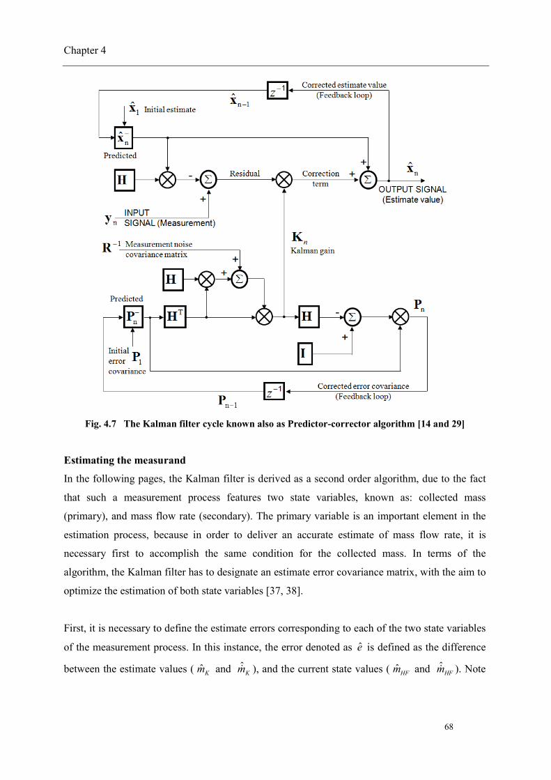
Chapter 4
68
Fig. 4.7 The Kalman filter cycle known also as Predictor-corrector algorithm [14 and 29]
Estimating the measurand
In the following pages, the Kalman filter is derived as a second order algorithm, due to the fact
that such a measurement process features two state variables, known as: collected mass
(primary), and mass flow rate (secondary). The primary variable is an important element in the
estimation process, because in order to deliver an accurate estimate of mass flow rate, it is
necessary first to accomplish the same condition for the collected mass. In terms of the
algorithm, the Kalman filter has to designate an estimate error covariance matrix, with the aim to
optimize the estimation of both state variables [37, 38].
First, it is necessary to define the estimate errors corresponding to each of the two state variables
of the measurement process. In this instance, the error denoted as e is defined as the difference
between the estimate values ( ˆ Km and ˆKm ), and the current state values ( ˆ HFm and ˆ
HFm ). Note

Chapter 4
69
that the term estimate error is used instead error, to underline the fact that there is no absolute
certainty in the true measurand value. Therefore,
ˆ ˆ ˆ HFm Ke m m (4.34)
ˆ ˆˆ f K HFe m m (4.35)
As the Kalman filter algorithm implies matricial operations, the estimate error is represented as:
ˆˆ
ˆ m
f
ee
e (4.36)
Now, in order to use the knowledge of the state variable estimate errors for the accurate
estimation of the measurand, the Kalman filter uses the covariance matrix as a statistical measure
to realize the degree in which these two state variables change or vary together. From the
covariance analysis, three important statistical assumptions of state variable association can be
made [39]:
1) If the covariance turns out to be positive, then it is inferred that both state variables vary
together in the same direction relative to their expected values,
2) The covariance is negative, if one of the state variables tends to be above its expected value,
meanwhile the second state variable is below its expected value, and
3) If the covariance is zero, then the variables are said to be statistically independent.
Hence, the covariance of the two state variables is represented in a matricial form by Eq. 4.37,
wherein the diagonal of the matrix represents the variance of collected mass and mass flow rate.
2
2
ˆ ˆ
ˆ ˆ ˆˆ ˆ ˆ
T
m m f
f m f
=
e e ee e e
P e e
(4.37)

Chapter 4
70
As for the initial estimate error covariance matrix, this can be obtained by substituting the
collected mass 1 1ˆ ( )HFm t t , mass flow rate 1
ˆ ( )HFm t at the time step 1 0t , in addition to
reference values Km and Km ,into the estimate errors shown in Eq. 4.34 and Eq. 4.35. On the
other hand, at the initial stage of the filtering process, the covariance terms of the matrix are set
to 0. The latter is due to the lack of information to set an accurate correlation level at this
particular time, as well as giving a more conservative assumption of little or no correlation
between the state variables [40]. This is preferred to designating a relatively high covariance, that
in return could significantly delay the filter convergence. In any case, the Kalman filter algorithm
will predict and correct the variance and covariance terms of the matrix within the following
iterations.
1
1
2
1 2
ˆ ( ) 0ˆ0 ( )
m
f
e t=
e t
P (4.38)
The initial estimate of the primary state (water mass) could be agreed to be equal to zero,
assuming that the collection vessel is empty. However, in order to keep the mathematical
consistency in terms of the second variable derivative, it is preferred to assignate a small value,
such as 1Km t . For the second state variable, it is possible to designate an arbitrary value for the
initial mass flow rate. Nevertheless, the usage of the average mass flow rate value given by
hydrodynamic force filter (Eq. 4.24) turns out to be a good initialization.
11ˆ Kx t = m t (4.39)
1ˆ( ) Kx t = m (4.40)
Then, according to Eq. 4.29, the predicted (a priori) state estimate can be described as:
=
= =S SK K K
K K
-n n-1
n-1 n-1 n-1
n-1 n-1
m (t )1 t m (t )+m (t ) tm (t )0 1 m (t )
x A x
ˆ ˆˆˆ ˆ
ˆ ˆ(4.41)

Chapter 4
71
In the current implementation of the Kalman filter, the measurement noise covariance R
(Eq. 4.42) is possible to be estimated, because the user is able to analyze the variance (Eq. 4.43,
Eq. 4.44 and Eq. 4.27) from data sets once the measurements are completed (off-line) [36 and
40]. Alternatively, such a standard deviation can be expanded in terms of its measurement
confidence interval [41], with the aim to increase the certainty in the estimate values.
2m2f
σ=
σ
R (4.42)
2
2
11
1 ˆ ( )N
m HF n n K nnN
m t t m t
(4.43)
2 2f HF (4.44)
Now with all the necessary information gathered, it is possible to derive the predicted covariance
equation shown in Eq. 4.30 as well as the corrected measurement equations (Eq. 4.31, Eq. 4.32,
and Eq. 4.33). Fig. 4.8 illustrates in a scalar form, the estimation process of mass flow rate via
Kalman filter. Hence:
Therefore, the a priori state error covariance matrix is:
11 12
21 22
22 21 12 11 22 12
22 21 22
- Tn n-1
2n-1 s n-1 n-1 s n-1 n-1 s n-1
n-1 s n-1 n-1
- -n n
- -n n
= =
p t + p + p t + p p t + p=
p t + p p
p p
p p
P AP A
(4.45)
The Kalman gain factor that is defined as:
11 11
21 11
-1- T - Tn n n
-1- - 2n n m n
-1- - 2 nn n f
+
+
p p σ k=
kp p σ
K = P H H P H + R
11
21
(4.46)

Chapter 4
72
The posteriori state error covariance matrix:
= -
11 11 11 12
21 21 11 22 21 12
-n n n
- -n n n n
- - - -n n n n n n
1 - k p 1 - k p=
p - k p p - k p
P I K H P
(4.47)
And the a posteriori state estimate is then:
=
m
m
m
11
21
11
21
- -n n n n n
nK n-1 K n-1HF n
K n-1 K n-1n
K n-1 n HF n K n-1
K n-1 n HF n K n-1
+ -
km (t ) m (t )(t ) 1 0
m (t ) m (t )k
m (t )+ k (t ) - m (t )=
m (t )+ k (t ) - m (t )
x x K y H x
ˆ ˆ ˆ
ˆ ˆˆˆ ˆ
ˆˆ ˆˆ ˆ ˆ
(4.48)
Fig. 4.8 Block diagram describing the estimation of mass flow rate via Kalman filter
(scalar form representation)

Chapter 4
73
4.3 SummaryIn this chapter, an inverse-problem approach with two algorithms has been presented, in order to
estimate the time-varying mass flow rate. The first algorithm is in charge of filtering out the
negative influence of the hydrodynamic and the buoyancy force variables have upon the
measurand. In order to do this, the filter uses the balance signal response as input signal, in
addition to an analytical model to estimate the magnitude of such unwanted forces, based on the
physical properties of the fluid, the geometry and dimensions of the system, and time. The
second algorithm is a filter, which attenuates the measurement noise still embedded in the signal
coming from the first filter. In this research work, the measurement noise is assumed to be
greatly caused (but not entirely) by the fluid force-induced oscillatory motion of the weighing
system. In this case, three data processing algorithms (central moving average filter, least-mean-
Square adaptive filter, and linear Kalman filter) have been proposed for the treatment of
corrupted signal. The central moving average filter that smoothes out the trend of the measurand
by using a series of data subsets averages, which are defined by a number of measurement data
before and after the current time step nt . The Least-Mean-Square adaptive filter adapts to the
input signal by iteratively tuning its parameters (filter coefficients), in order to deliver an
estimate measurand value with a minimized feedback error signal. The linear Kalman filter
combines the knowledge of the weighing system output signal (i.e. variance) and its recursive
method to produce a mass flow rate estimate value. In the following Chapter 5, the performance
of the proposed measurement noise filters will be numerically assessed in terms of their
stabilization time, accuracy, precision, and their ability of reproducing consistent results at
different stationary and quasi-steady mass flow rates.

Chapter 5
74
5. Numerical determination of mass flow rate and the response of
the dynamic weighing liquid flow standard
The dynamic simulation of the weighing system is the basis for understanding or exemplifying,
which fluid and mechanical phenomena are taking place, finding out the sources of measurement
noise, the unwanted variables involved, and realizing which variables are the most relevant in the
measuring process. Furthermore, a comparison between the numerical and the real process
measurements is carried out, with the aim to validate the theoretical background of the
measurement process model as well as the mass flow rate calculation via dynamic-weighing.
The numerical analysis shown in this document firstly evaluates the system´s input signal, and its
frequency response. The next step comprises the simulation of the continuous time system
response (Chapter 3), followed by the oscillatory signal attenuation of the low pass filter, and
the discrete time representation of the output signal. The latter is compared with the balance
readout, in order to see the level of agreement. Afterwards, the effectiveness of the
hydrodynamic force filter is numerically evaluated, so then its contribution to the measurement
accuracy can be quantified.
The second part concerning to data processing techniques, addresses the performance of three
proposed measurement noise filters. The assessment is focused on their capabilities to enhance
the measurement accuracy and precision as well. Finally, the numerical analysis evaluates the
role that the data sampling frequency as well as the low-pass-filter cutoff frequency, play upon
the measurand estimates; and it suggests a possible way to re-enhance the accuracy. Fig. 5.1
summarizes in a block diagram all the recalled steps for the estimation of the mass flow rate via
dynamic weighing. As a reminder (Chapter 3), qF (t) denotes the fluid forces caused by the
vortex axial force inside the collection vessel and the oscillatory force of the water waves. In this
numerical analysis, qF (t) is not taken into account, because none equation has been derived to
describe their behavior. Nevertheless, it is reminder that such forces have to be considered in
subsequent investigations, so that a more thorough system model can be achieved.

Chapter 5
75
Fig. 5.1 Block diagram describing the steps made for the simulation of the mass flow rate estimate
via dynamic weighing
5.1 Fluid forces acting upon the weighing system (input signal)As recalled, the input signal of the measurement process does not comprise a single physical
variable, but a summation of three predominant forces, which in part, dictate the dynamic
behavior of the system. In this instance, the simulations of time-varying fluid force magnitudes
are exemplified at the lowest and highest flow rates attained by the dynamic weighing liquid
flow primary standard prototype (Fig. 5.2), which is described in full detail in Chapter 6.
Additionally, the vessel is assumed to be empty, whereby the initial collected water mass is zero.
In regards to the hydrodynamic force dF (t) shown in Fig. 5.2, this exhibits a proportional
increment in its magnitude in relation to the operational mass flow rate, and an inverse response
to the level rise of the collected water.
As for the collected water mass force mF (t) , it can be described as a ramp-function like variable,
wherein its magnitude is the product of its slope (the current mass flow rate), the time t of the
measurement, and its initial value agreed to be zero. As a remark, the level of filling in these
simulations is carried out at 80% of the vessel nominal capacity (8 L).

Chapter 5
76
Fig. 5.2 Fluid forces acting upon the weighing system (Input signals)

Chapter 5
77
It is worth to highlight that, the time-varying mass flow rate data used to carry out all simulations
are extracted from the experimental data given by a flowmeter used as a reference standard. This
is intentionally done, with the aim to approximate the real conditions undergone by the physical
system (Chapter 6).
Concerning to the buoyancy force bF (t) , this acts as a function of the water mass and in an
upward direction, therefore its response is seen in Fig. 5.2 as a positive slope. Furthermore, in a
dynamic weighing condition, the buoyancy force is by no means influenced by the inertial mass
force, but only by the air density, water density, the local acceleration of gravity, and the
increasing collected water mass. For the sake of simplification, the density of air and water is
assumed to be constant at a reference temperature of 20°C.
The summation of these forces yields what is called, the total fluid force TF (t) . In Fig. 5.2, such
a variable is intentionally compared with the collected mass force, in order to show their
difference in terms of magnitude. As expected, the magnitude difference (or slope shift) between
TF (t) and mF (t) becomes more significant as the mass flow rate increases.
The two lower graphs at 3 kg/min and 8 kg/min in Fig. 5.2 also illustrate the magnitude ratio
between the hydrodynamic force - buoyancy force ( d bF (t) - F (t) ), and the collected mass force,
mF (t) . Such a ratio helps to visualize the considerable systematic error involved, when simply
considering the balance output response as an estimate mass to calculate the current flow rate.
Additionally, Fig. 5.2 shows that the influence of dF (t) and bF (t) are quite strong during the first
1/3 of the filling process, and especially at the highest flow rate. Thereafter, such a ratio curve
exhibits an exponential decay of the hydrodynamic and buoyancy force influence upon the
measurement process, which can be as low as 0,1% at 3 kg/min.
5.2 Frequency response of the weighing systemThe aim of this task is to apply a Fast Fourier Transform (FFT) in order to find out the balance
frequency response upon its weighing axis (z axis), and how this behaves along the measuring
time. This kind of information is important to be known because in practice, the weighing system
features a low pass filter, which uses such frequency information, in order to define the
attenuation level of the output signal. As understood, the low pass filter is an algorithm, which

Chapter 5
78
balance manufacturers commonly use, with the purpose to diminish the amplitude of the system
oscillatory force from the output signal. The latter is an unwanted signal considered as
measurement noise. In the simulation work, the characterized balance oscillatory frequency will
be used by the low pass filter of the numerical model (Chapter 3), as an attempt to reproduce the
real attenuated output signal displayed by the balance readout.
The balance frequency characterization consists of applying a non-contact laser displacement
sensor (LDS) [1] to measure the oscillatory displacement of the balance platform at two different
planes, as depicted in Fig. 5.3. The reason for measuring at two different planes (XZ and YZ) is
in order to characterize the eigenfrequencies generated by the translational and angular motion of
the balance platform during the measurement process, and thus, to identify which one
corresponds to the z axis oscillatory motion [2]. Note that, if this eigenfrequency characterization
were carried out at one plane, the result might possibly lead to an overlooking of an
eigenfrequency, including the one belonging to the z axis, which could be only detected at one
particular plane. In addition to the non-contact laser displacement sensor, an accelerometer is
also mounted upon the balance platform and oriented along the z axis, with the goal to
corroborate the results from the first method (LDS), regarding the weighing axis frequency
identification.
Fig. 5.3 Setup of the weighing system frequency characterization test
After carrying out the experimental tests, the results revealed three frequency spectra that are
present in a bandwidth of 24 Hz, wherein the lower and upper limits are respectively, 9 Hz and
33 Hz. The explanation to the frequency response decay and magnitude observed in Fig. 5.4

Chapter 5
79
(regardless the motion axis) is predominantly based upon the stiffness coefficient of the
weighing system, and the continuous increment of the system mass caused by the collected
water.
Fig. 5.4 Three frequency spectra taking place during the filling process at 3, 5 and 8 kg/min and
their power spectral density at an estimated collected mass of 4 kg
As depicted in Fig. 5.4, such a frequency response is agreed to behave nearly in the same
manner, even if the weighing system operates at a low, medium, or large mass flow rate.
Chapter 5
80
Moreover, after comparing the results obtained by the non-contact displacement sensor and the
uniaxial accelerometer (Fig. 5.4), it points out that the eigenfrequency of the weighing axis (z
axis) is ranging between 33 Hz and 29 Hz, because of the near overlapping between the two
different measurement approaches. As a remark, the z axis eigenfrequency was detected at both
planes (XZ and YZ), and with a relatively higher amplitude of its spectrum, in comparison to the
other two eigenfrequencies (Fig. 5.4).
Note that the term estimated collected water mass in Fig. 5.4 is used, because the system
frequency characterization was carried out dynamically [3]. This means, that the
eigenfrequencies were tracked during the collection process, and the mass had to be calculated as
an estimate by using Eq. 5.1 (see Chapter 4) and Eq. 5.2.
2
( )
( )( )
( )
( )
ˆ ˆ ˆ
ˆ
A
ww
A
w
AHF n HF n
w
ABal n n HF n Bal n
w
24 2 2 2
i n2 2w n
1 m (t )+ 2 g h (z) g 1- t m (t )+...ρ A
...+ 2 F (t ) g 1- t m (t ) F (t )=0
(5.1)
ˆˆ HF HFn n nm (t ) m (t ) t (5.2)
Another important conclusion made after analyzing the system´s mechanical frequency response
is the presence of the oscillatory transverse forces upon the x axis and y axis (Fig. 5.3 and
Fig. 5.4), produced by the radial spread of the submerged water jet [4]. This would indicate that
the system is subjected to move in more than one degree of freedom (rotational and/or
translational), and that not only the system´s mass but also the system´s moment of inertia
around the x and y axes, play a role in the dynamic response of the balance.
An additional assumption extracted from the results in Fig. 5.4 is the fact that at least two
oscillatory transverse forces are superimposed in the balance output signal [5]. Eventually, their
magnitudes are in principle much smaller, because as illustrated in Fig. 5.3 and Fig. 5.4, the
main driven force is acting upon the normal axis (z axis). On the other hand, from the point of
view of the balance sensing element, this will be able to measure exclusively (theoretically) the
force oriented upon the weighing axis (z axis). However, due to its inherent transverse sensitivity [6],
a small residual force (even negligible in some cases) from the flow-induced radial forces

Chapter 5
81
will be measured and displayed. The impact of the transverse sensitivity upon the balance
readout is mainly a function of the particular mechanical design of a weighing sensing element
(cell), the mechanical coupling between balance weighing platform and its cell, the magnitude of
the radial fluid forces, the balance positioning control system [7], the internal low pass filter and
the data sampling rate of the output signal. This characteristic of the system can be named as a
mechanical crosstalk effect, due to the fact that an unwanted signal(s), in the case of radial
forces, can be superimposed in the balance readout.
In this research work, one of the main goals was to find out the main phenomena (mechanical
and fluid aspects) that greatly affect the system, and an accurate estimation of mass flow rate.
For this reason, the system is analyzed with respect to the axis, wherein the main acting fluid
force and balance dynamic response is taking place, the z axis. Nevertheless, the mechanical
cross talk effect is intentionally mentioned in this chapter, as a hint for a future investigation
related to a more thorough understanding and accuracy enhancement of a dynamic weighing
liquid flow primary standard (Multi-axis weighing system model). Eventually, this further
investigation will have to include the identification task of the other two eigenfrequencies
(Fig. 5.4), with their corresponding system´s degrees of freedom.
5.3 Continuous time and discrete time response of the balanceFig. 5.5 shows the balance simulated response during the filling process. As shown in the upper
graph of Fig. 5.5, the balance output response is depicted in its continuous time form. According
to the numerical calculations, the output signal follows the path of the total fluid force, in
addition to an oscillatory signal caused by the balance reacting dynamic response. The graphs
depict a nominal undesired oscillatory signal of 33 Hz (at the initial stage of the process), and
with a maximum amplitude of ±0,5 N at 8 kg/min, and ±0,2 N at 3 kg/min.
According to the weighing system signal conditioning, the continuous time balance response
must undergo a decrement in its oscillatory amplitude. Hence, a low pass filter uses the
frequency response upon the z axis to define the attenuation level of the signal [8]. In this
instance, the eigenfrequency ranging from 33 Hz to 29 Hz is out of the low pass filter pass band,
which features a cutoff frequency of 10 Hz [8].

Chapter 5
82
Fig. 5.5 Simulation of the continuous and discrete time dynamic response of the balance at8 kg/min (upper graph) and 3 kg/min (lower graph)

Chapter 5
83
Moreover, the numerical outcome given by the low pass filter depicts a continuous time signal
that has been attenuated from -11 db to -9 db, due to the eigenfrequency decrement along the
filling process, and with a signal phase shift between 73° and 71°, as shown in Fig. 5.6. Herein,
the simulated original signal has continuously changed, not only in terms of its oscillatory
amplitude, but also in relation to its frequency and phase [9].
Fig. 5.6 Low pass filter gain and phase shift of the weighing system model
The last step before displaying the measured reacting force is to convert it into a discrete time
form. In this case, the designated data sampling frequency of the balance is 30 Hz [8] observed
in Fig. 5.5, the original continuous time balance output signal has experienced a serious aliasing
effect [10] after passing through the low pass filter, and the discrete time conversion.
Nevertheless, the signal is still valuable because it continues following the path (or slope change)
of the total fluid forceT
F (t) . As mentioned in Chapter 4, the total fluid force is one of the key
variables used in the process model (Hydrodynamic force filter) to calculate the mass flow rate
estimates.
Finally, the simulated output response of the weighing system is compared with its experimental
counterpart, the balance readout. For instance, Fig. 5.7 shows the start point of the measurement
process at 8 kg/min, wherein the experimental data depict an initial signal overshoot, greatly

Chapter 5
84
caused by the first shock of the water jet upon the vessel [11]. This overshoot response depicted
in Fig. 5.7 was not replicated by the simulation, nevertheless, the initial step and the subsequent
ramp response agree with the experimental part. Furthermore, the simulated signal in both mass
flow rates (8 kg/min and 3 kg/min) yields a discrete-time oscillatory response, which is fairly
similar in magnitude, with the one measured experimentally.
As mentioned, the numerical model uses the mass flow data provided by the PTB traceable
transfer standard (flowmeter), with the aim to replicate as close as possible the quasi-steady and
quasi-uniform mass flow rate.
Fig. 5.7 Numerical and experimental comparison of the balance weighing axis eigenfrequency andits discrete-time output signal response at 8 kg/min (upper graph) and 3 kg/min (lower graph)

Chapter 5
85
5.4 Hydrodynamic force filterIn this instance, the hydrodynamic force filter is applied at three different mass flow rates, with
the goal to see its effectiveness in approximating to the average value of the true measurand, or
in other words, improving the measurement accuracy.
At 8 kg/min, two different calculation approaches are compared. One is the mass flow rate
obtained by directly using the force measurements given by balance readout, time, and the local
acceleration of gravity (Eq. 4.1). The result from this estimation method delivers a series of
measurements that are quite spread along its average value (±0,2 kg/min at 5s, or a maximum
relative error of ±2,43% with respect to its average value), but they gradually decrease until
±0,25% at 55s. As illustrated in Fig. 5.8, the difference between the average value obtained by
this approach and the average reference mass flow rate is 0,24%.
The second approach depicted in Fig. 5.8 is the outcome given by the Hydrodynamic force filter,
already described in Chapter 4. In regards to its performance, the data spread is similar to the
first approach (Balance readout), due to the fact that such a filter treats only the accuracy of the
whole measurement data, but not their precision. That is exactly the task of the measurement
noise filter, in which their numerical results are presented in the next section. According to the
attained results, the average value of hydrodynamic force filter output signal is able to get really
closer to the true measurand. The percent relative error found at this flow rate was 0,01%.
A similar output signal response takes place at the mid flow (5 kg/min), wherein the scattered
data at the initial stage of the measurement (10s) exhibit a percent relative error of 1,35%. As
demonstrated from the highest and mid flow rate, the degree of data scattering is proportional to
the operational mass flow rate. On the other hand, when comparing the outcome given by the
two measurement approaches, it is clear that the hydrodynamic force filter enhances the accuracy
of the mass flow rate estimate values about 5 times in relation to its counterpart.
The results at the lowest flow rate can be seen as an affirmation of the two filters response,
wherein the dispersion of data is lower (i.e. 0,67% relative error at 20s) as the mass flow rate
decreases. For a detailed explanation of this process condition, see Section 5.1 (specifically
Fig. 5.2), regarding to the fluid forces acting upon the weighing system.

Chapter 5
86
Fig. 5.8 Response of hydrodynamic force filter and its effect upon the measurement accuracy
enhancement at 8, 5 and 3 kg/min

Chapter 5
87
5.5 Proposed measurement noise filters
5.5.1 Central moving average filter
Fig. 5.9 shows the measurand tracking performance of the central moving average filter at the
highest mass flow rate (8 kg/min). In this figure, the results show that 23 of 28 estimating values
are moving along the average mass flow rate value (8,227 kg/min), and overlapping several
times the true time-varying mass flow rate. As a remark, the number of samples used to calculate
each of the estimate points was 490 samples.
A particular behavior observed from this filter output is that the estimate values are barely
following the path of the true mass flow rate, especially at the second half of the collection time.
However, this apparent limitation is compensated by the fact that the error band of the estimate
values with respect to the true measurand is in the order of ±0,025%.
At 5 kg/min, the central moving average filter converges after 12.5s, wherein 25 of 30 estimate
values are within an error band of ±0,02%, with relation to the true time-varying mass flow rate.
In this instance, the central moving average filter is able to only coincide with the average of the
measurand, but also to carry out a better tracking of the transient flow response.
With regard to the lowest mass flow rate, the central moving average took about 1/10 of the
measurement time to stabilize, and thus getting 54 of 58 estimate values within an error band of
±0,03%. Furthermore, it is worth to observe in Fig. 5.9, that despite the non-exact estimation of
the central moving average, it follows the ascending and descending path of the time-varying
mass flow rate.
One common characteristic found out after analyzing the response of the central moving average
(at three different mass flow rates) is: the overshoot response appearing at the initial stage of the
filter estimation process, which seems to have a strong correlation with the large measurement
variance (Hydrodynamic force filter output signal), originated by the dynamic mechanical
response of the weighing system. Moreover, the settling time of 12.5s was consistently repeated
at the three different flow rates, suggesting that this behavior might be independent of the
measurement data, but related to the filter algorithm and its parameters.

Chapter 5
88
Fig. 5.9 Performance of the central moving average filter at 8, 5 and 3 kg/min

Chapter 5
89
5.5.2 Least-Mean-Square adaptive filter
At the highest flow (8 kg/min), the adaptive filter presents an initial response delay of 2,5s
(Fig. 5.10), caused by the decorrelation of its input signal (Chapter 4, Section 4.2.2), and the
number of filter coefficients (500) used to minimize the measurement noise. On the other hand,
the adaptive filter uses as an initial estimate, the average mass flow rate magnitude yield by the
hydrodynamic force filter, which according to Fig. 5.10 turns out to have an accuracy of
approximatelyt 0,01%.
During the estimation process, the filter takes approximately 1/3 of the total measuring time
(20s) to smoothly reach an estimate within ±0,05%. As shown in Fig. 5.10, the non-overshoot
convergence response of the filter denotes a stable and reliable estimation process, which is
associated with the number of filter coefficients in use, and the designated stability fraction of
the signal error (Chapter 4, Section 4.2.2). Finally, the outcome given by the adaptive filter at
8 kg/min yields a set of 8750 estimate values.
As for the measurements carried out at 5 kg/min, the adaptive filter takes also 1/3 of the nominal
measuring time to converge, within ±0,04%, in relation to the average mass flow rate
(5.1815 kg/min). After the second half of the filling process, some of the estimate values are
overlapping and keeping a good tracking of the true measurand; especially between the time 50s
and 80s. According to the obtained results, the number of estimates after the filter stabilizes is
approximately 13750.
Concerning to the lowest flow, Fig. 5.10 points out that the adaptive filter required about 1/4 of
the total measuring time to stabilize with a non-overshoot response. After the first half of the
process time, the adaptive filter was able to obtain about 25000 estimates that mostly follow the
average mass flow rate of 3,279 kg/min, within a band of ±0,03%.
The adaptive filter as well as the moving average (Fig. 5.9 and Fig. 5.10) seems to be affected by
the influence of the relatively large measurement noise taking place at the first 1/3 of the process
time. One main reason of such a common behavior is that both algorithms utilize a weighted
sum, in order to determine their estimate values. In other words, the estimates at the initial part of
the process are subjected to deliver more inaccurate values, because of the large measurement
variance, and the low magnitude of its statistical weight (reliability).

Chapter 5
90
Fig. 5.10 Performance of the Least-Mean-Square adaptive filter at 8, 5 and 3 kg/min

Chapter 5
91
5.5.3 Linear Kalman filter
At 8 kg/min, the Kalman filter rapidly approaches to the true time-varying mass flow rate. The
largest difference found between both measurement data was 0,1% during the first second of the
estimation process (Fig. 5.11). A particular characteristic observed in the Kalman filter response
is that besides following the quasi-steady mass flow rate, its scattered data serve as a band that
covers the measurand all along the measuring time. The same type of response occurs for the two
following flow rates at 5 kg/min and 3 kg/min. From this numerical test, the Kalman filter was
able to perform an approximate of 11250 accurate estimates after 10s.
In relation to the mid flow, the estimate values as well as the true value were very relative more
uniform through the measuring time than the outcome data at 8 kg/min and 3 kg/min. In this
instance, the estimate data are spread in a range of ±0,02% after 30s. Moreover, as shown in this
graph and the one at 3 kg/min, the Kalman filter demonstrates its ability to rapidly minimize the
variance in its estimate error, as well as attenuating the large amplitude measurement noise
during the initialization phase.
At 3 kg/min, the reference measurements exhibit a clear decrement of 0,03% with respect to its
initial value. However, this process condition does not represent a major problem to the Kalman
filter algorithm, as it is capable to follow the same flow trend with a maximum relative
difference of only 0,02% at 50s.
The average mass flow rate (hydrodynamic force filter output signal) was used not only by the
adaptive filter algorithm, but also by the Kalman filter to set its initial estimate. Hence, as a
result, the estimate values can converge the reference data with less number of iterations. As
recalled, the last statement is applicable, because the process is intended to be performed at a
steady flow condition. Furthermore, when comparing the performance of the three proposed
filter, it is concluded that the Kalman filter delivers the largest number of estimate data with the
lowest relative error.

Chapter 5
92
Fig. 5.11 Performance of the Linear Kalman filter at 8, 5 and 3 kg/min
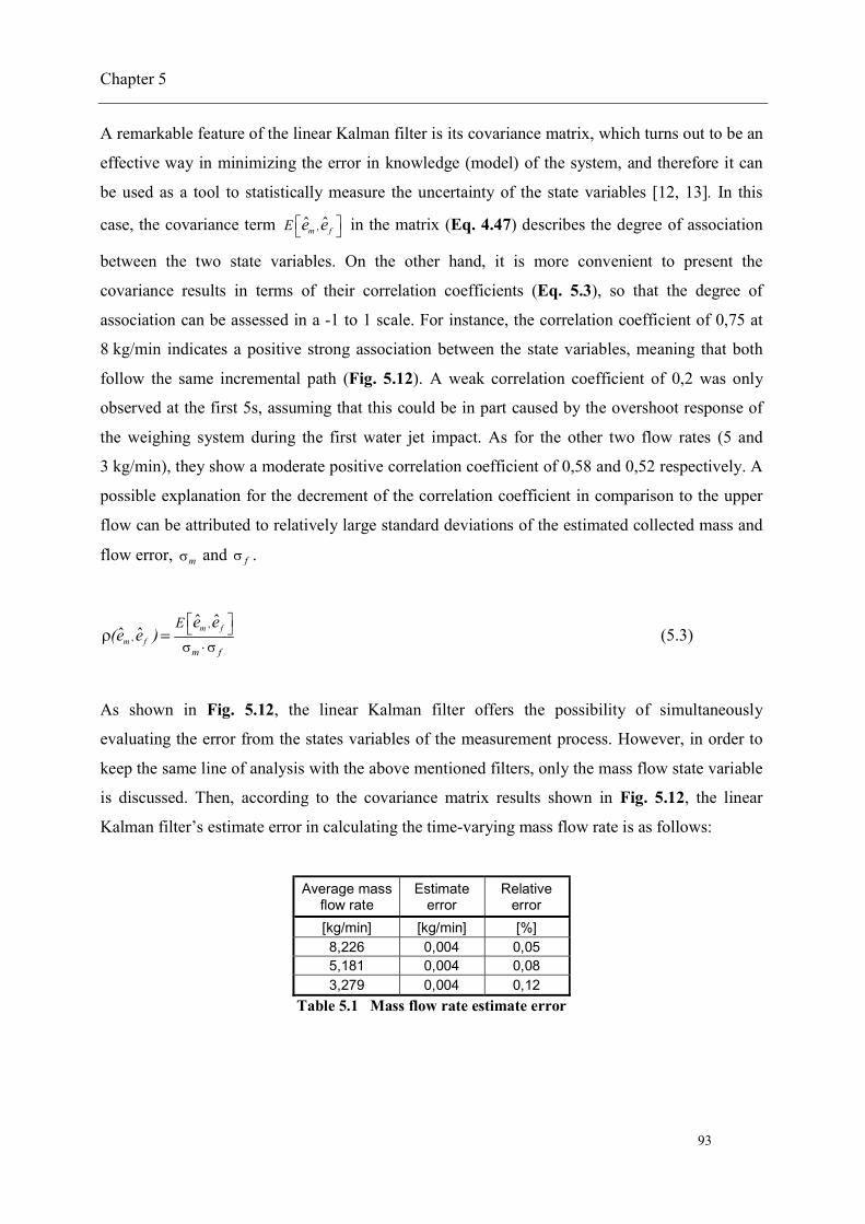
Chapter 5
93
A remarkable feature of the linear Kalman filter is its covariance matrix, which turns out to be an
effective way in minimizing the error in knowledge (model) of the system, and therefore it can
be used as a tool to statistically measure the uncertainty of the state variables [12, 13]. In this
case, the covariance term ,ˆ ˆm fE e e in the matrix (Eq. 4.47) describes the degree of association
between the two state variables. On the other hand, it is more convenient to present the
covariance results in terms of their correlation coefficients (Eq. 5.3), so that the degree of
association can be assessed in a -1 to 1 scale. For instance, the correlation coefficient of 0,75 at
8 kg/min indicates a positive strong association between the state variables, meaning that both
follow the same incremental path (Fig. 5.12). A weak correlation coefficient of 0,2 was only
observed at the first 5s, assuming that this could be in part caused by the overshoot response of
the weighing system during the first water jet impact. As for the other two flow rates (5 and
3 kg/min), they show a moderate positive correlation coefficient of 0,58 and 0,52 respectively. A
possible explanation for the decrement of the correlation coefficient in comparison to the upper
flow can be attributed to relatively large standard deviations of the estimated collected mass and
flow error, m and f .
,,
ˆ ˆˆ ˆ m f
m fm f
E e e(e e )
(5.3)
As shown in Fig. 5.12, the linear Kalman filter offers the possibility of simultaneously
evaluating the error from the states variables of the measurement process. However, in order to
keep the same line of analysis with the above mentioned filters, only the mass flow state variable
is discussed. Then, according to the covariance matrix results shown in Fig. 5.12, the linear
Kalman filter’s estimate error in calculating the time-varying mass flow rate is as follows:
Average massflow rate
Estimateerror
Relativeerror
[kg/min] [kg/min] [%]8,226 0,004 0,055,181 0,004 0,083,279 0,004 0,12
Table 5.1 Mass flow rate estimate error

Chapter 5
94
Fig. 5.12 Linear Kalman filter estimate error variance and correlation coefficient at
8, 5 and 3 kg/min

Chapter 5
95
5.5.4 Summary
Central moving average
The highly corrupted measurement noise present in one or more samples enclosed in a data
set increases the measurement variance, and as a consequence, considerably affects the
accuracy of the central moving average calculation,
The central moving average filter shows an initial overshoot, which is later overcome by a
smoother and more accurate estimation response,
The moving average estimation process yields a limited number of estimate values in relation
to its counterparts, the LMS adaptive and the linear Kalman filter. However, such a number
can be sufficient or even larger, if compared with the number of data samples (usually from 5
to 10 measurement points) required in a regular calibration task [14].
LMS Adaptive filter
As noted in the series of simulations, the adaptive filter features neither an overshoot nor an
unstable system response. This is achieved at the expense of a considerable time taken in
order to converge the reference values,
The LMS adaptive filter as well as the moving average filter seem to be affected by the
influence of the relatively large measurement noise taking place at the first 1/4 of the process
time. One main reason of such a common behavior is that both algorithms utilize a weighted
average (with their corresponding filter coefficients) in order to determine their estimate
values. In other words, the estimates at the initial part of the process are subjected to deliver
more inaccurate values because of the large measurement variance, and hence a lower
statistical weight (reliability) [15].

Chapter 5
96
Linear Kalman filter
As shown in the simulation results, the Kalman filter benefits from its recursive property
with no need of storing past measurements for the purpose of computing its present estimate
(but only its previous step). This feature makes possible the rapid minimization of the
variance in its estimation error, a less stiff response to sudden changes of the measurand, and
ultimately, more time-varying accurate estimates,
The usage of the average mass flow rate magnitude (coming from the Hydrodynamic force
filter) as a basis for the measurand estimation is a key parameter the Kalman filter employs to
obtain a reliable estimate response in less iterative cycles. The last statement is applicable
because the process is intended to be performed at a quasi-steady and stationary flow
condition.
5.6 The influence of the data sampling frequency and the low pass filter
cutoff frequency upon the mass flow rate estimate values and its
measurement accuracy enhancementWhen dynamic weighing mass flow measurements are performed experimentally, the outcome is
at some degree limited by the manufacturer design specifications. In this instance, it is referred to
the maximum data sampling frequency the balance readout can deliver, and the internal filter
algorithm (low pass filter) used to attenuate the undesired oscillatory response of the balance.
The following section analyzes numerically the effects of the data sampling frequency as well as
the low pass filter upon the measurand, by changing their parameters. The main goal of
comparing these results is to have some understanding about the factors that negatively
contribute in the determination of the measurand, and what can be done in practice, in order to
bring more accurate and precise mass flow rate measurements.
In principle, any of the recalled measurement noise filters could be used to evaluate the
measurand response under the different measurement parameters previously mentioned.
However, it is more appropriate to select in this case the Kalman filter, because according to the
numerical and experimental (Chapter 6) results, it is the one that stabilizes faster, it is accurate
in its response, and in general, it is capable to follow more effectively the time-varying mass
flow rate.

Chapter 5
97
The numerical analysis is divided into three aspects:
The measurand response is evaluated at two different mass flow rates, at three different data
sampling frequencies, and at a low pass filter cutoff frequency of 10 Hz, which is equal to the
value set up in the balance (Fig. 5.13),
The measurand response is assessed at two different data sampling frequencies, and at three
different low pass filter cutoff frequencies (Fig. 5.14 and Fig. 5.15), and
To analyze the characteristics of a mass flow rate measurement at two different data sam-
pling frequencies, with the absence of a low pass filter (Fig. 5.16).
In Fig. 5.13, the results of the mass flow rate estimate values are presented at 8 kg/min and
3 kg/min, with a data sampling frequency of 10 Hz, and a low pass filter cutoff frequency of
10 Hz (see upper graphs). In this example, both flow rates present a measurand response, which
lasted about 1/3 of the process time to converge the true mass flow rate value. The maximum
relative errors between the estimated values, and the true values at the first stage of the process
were in the order of 0,085% at 8 kg/min, and 0,092% at 3 kg/min. Remember, that the term true
value is valid (at least numerically), because it is a known input quantity introduced in the model.
This is a clear example of how not only the fluctuating flow but also a limited data sampling
frequency can affect the ability of a filter to estimate the measurand. This is especially a concern
in the regions where the amplitude measurement noise is relatively high.
The two mid graphs at 8 kg/min and 3 kg/min in Fig. 5.13 show the estimate values at a low pass
filter cutoff frequency of 10 Hz, and an increased data sampling frequency of 30 Hz. The 30 Hz
magnitude of the data sampling frequency is intentionally assessed in order to try to reproduce
the response of the system at its current set up. The graphs clearly describe a prompt
convergence of the estimate values, despite the larger data spread at the beginning of the process.
This initial behavior can be associated with the influence of the large measurement noise.
The two simulations carried out at a data sampling frequency of 90 Hz show a particular
behavior in terms of the fast stabilization time and the spread of the estimated data, which turn
out to be very homogeneous along the time (0,01%).

Chapter 5
98
Fig. 5.13 Simulation of the balance output signal response (8 kg/min and 3 kg/min) at a data
sampling frequency of 10 Hz, 30 Hz and 90 Hz, and a fix low pass filter cutoff frequency of 10 Hz

Chapter 5
99
As seen in Fig. 5.13, the response of the estimation process describes a quite similar behavior
regardless of the mass flow rate. Therefore, the analysis can be dedicated to one mass flow rate.
Fig. 5.14 summarizes the performance of the estimation task at three different low pass filter
cutoff frequencies (5 Hz, 10 Hz and 20 Hz) at 30 Hz in relation to its data sampling frequency.
The measurements performed at three different cutoff frequencies present a common response in
terms of estimation path. On the other hand, Fig. 5.14 also indicates that the level of coverage
from the estimate values (seen as data spread) is proportional to the cutoff frequency. This can be
expected, because the low pass filter yields higher attenuation levels at small cutoff frequencies,
as happens, for instance, at 5 Hz.
Fig. 5.15 describes the simulated response of the Kalman filter to estimate the mass flow rate
when the balance sampling frequency is significantly higher (90 Hz), and at three different cutoff
frequencies. The outcome indicates that the influence of the measurement noise is minimal in all
cases because the larger number of data samples allows the filter to reduce, in less iterations, the
measurement variance. The upper graph (at 5 Hz) in Fig. 5.15 underlines an important fact that
besides attenuating the unwanted balance oscillatory force, the low pass filter takes part of the
measurand data. The overriding of measurand data is clearly seen when comparing the different
cutoff frequencies of the system. The wider the low pass filter´s pass band, the more accurate the
estimation.

Chapter 5
100
Fig. 5.14 Simulation of the balance output signal response at three different low pass filter cutoff
frequencies (5 Hz, 10 Hz and 20 Hz) and a data sampling frequency of 30Hz
Fig. 5.15 Simulation of the balance output signal response at three different low pass filter cutoff
frequencies (5 Hz, 10 Hz and 20 Hz) and a data sampling frequency of 90Hz

Chapter 5
101
Fig. 5.16 exemplifies the filter response when the low pass filter is excluded from the output
signal conditioning process. In this example, the estimated values at a balance sampling
frequency of 30 Hz are satisfactory, despite the apparent influence of the measurement noise at
the beginning of the measurement. On the other hand, the performance of the filter is outstanding
when the system is able to sample data at 90 Hz. In this case, the estimate values converge in a
few seconds after the start point of the collection process. Additionally, the filter keeps tracking
the fluctuated mass flow rate, within a band of 0,05% with respect to the average magnitude.
The conclusion given by this analysis is that the accuracy and precision of the estimate values
can be re-enhanced, if the balance output signal could skip the low pass filter, and the sampling
frequency would be higher [16]. However, the criteria for an appropriate increment of the data
sampling frequency will be closely related, for instance, with the level of stationary fluctuating
flow at the primary standard and the balance time constant. Furthermore, as an important remark,
these specific output signal characteristics can be currently provided only by customized balances.
Fig. 5.16 Simulation of the balance output signal response at a data sampling rate of 30 Hz and
90 Hz without low pass filter

Chapter 6
102
6. Experimental results
The content of this chapter addresses the theoretical, mechanical, and data acquisition set up of a
prototype used as a dynamic weighing liquid flow standard. Furthermore, it presents a series of
measurements performed at different mass flow rates, with the aim to experimentally determine
the accuracy level of the process model algorithm described in Chapter 4.
For these series of tests, the reference system in use is a flowmeter with direct traceability to the
PTB national standard for low liquid flow measurements [1]. This means, a measurement
approach, in which a primary flow standard can provide a low-uncertainty characterization to the
flowmeter output signal, and at the same time, a flowmeter that is capable of tracking the
stationary and quasi-steady mass flow rate fluctuation in small time intervals, but within the
uncertainty claimed after its calibration. The description of the transfer standard is also given in
this chapter.
6.1 Transfer standard used for the liquid flow comparisonThe transfer standard used for these experimental tests is a turbine flowmeter owned by the PTB
calibration laboratory, which complies with all metrological requirements of reproducibility,
repeatability, linearity, precision, and covers the measuring range demanded by the tests.
Regarding its working principle, the turbine flowmeter is a metering device, which converts the
mechanical angular velocity of the rotor (generated by the mass flow) into an electrical frequency
signal [2]. In other words, if the mass flow passing through the meter increases, the rotor angular
velocity as well as the electrical frequency measured by an external pickoff will raise in the same
manner (Fig. 6.1). Concerning its mechanical construction, the turbine rotor has to be held inside
the stream, whereby supports are added to position the rotor bearing in the pipe as shown in
Fig. 6.1. Additionally, such supports serve as a flow straightener that removes the swirls and/or
disturbing flows caused by upstream pipe fittings and valves. Another good feature of the turbine
meter is the high-sensitivity of the mechanical sensing element (rotor) to sudden changes of mass
flow rate during a measurement run [3 and 4], despite some small response delay attributed to a
retarding torque from the rotor [5].

Chapter 6
103
Fig. 6.1 Turbine flowmeter used as a transfer standard
The transfer standard is a 25-mm turbine flowmeter that has been previously calibrated by the
PTB primary standard of liquid flow, within 2 kg/min to 10 kg/min. The results of this
characterization are given in terms of a ratio called K factor, which represents the number of
pulses read by the pickoff during the transfer of 1 L of water through the flowmeter (Eq. 6.1).
The K factor of the transfer standard was defined to be equal to 12821 pulses/L, and on the other
hand, the region of linearity of this flowmeter was found between 3 kg/min and 8 kg/min. This is
the flow range that will be used during the measurement comparison, due to its relatively lower
measurement uncertainty levels and repeatable results.
MeterMeter
PTB
fK =
V (6.1)
Here Meterf denotes the turbine rotor frequency in Hz, and PTBV represents the volumetric flow rate
determined by the PTB primary flow standard during the characterization process. Meanwhile,
during the dynamic flow measurement tests, the turbine flowmeter will be able to calculate the
mass flow rate by using Eq. 6.2, which is a dependent function of the obtained turbine calibration
factor MeterK , nMeterf t , and the fluid density Meterwρ at its location.
31
Meter nw Metern
Meter
Meter
ρ f tm t =1000 LK
m
(6.2)

Chapter 6
104
As for the measurement uncertainty attributed to the transfer standard, this can be determined by
the combined measurement uncertainty of the small PTB liquid flow primary standard
(PTB
U 0,05% ) [1], in addition to the uncertainty of the transfer standard due to its repeatability
(Meter_Rep
U 0,06% ). Both values are referring to a 95% confidence level.
22
Meter PTB Meter_RepU = ± U + U
= ±0,078%(6.3)
On the other hand, the measurement uncertainty of the Dynamic Weighing Liquid Flow Standard
prototype (DWLFS) is estimated by the combined uncertainty of the storage effect of the
connecting volume CVU (Chapter 3), and the uncertainty related to the time-varying estimate
error given by the process model algorithm neU t .
22n nDWLFS CV eU t = ± U + U t (6.4)
6.2 Data acquisition systemThe data acquisition system and signal synchronization for the dynamic weighing liquid flow
standard prototype (DAQ) is realized by a software written in Labview®, and a programmable
automation controller known as NI CompactRIO® [6]. Such equipment comprises a dedicated
400-MHz microprocessor that serves to acquire synchronous real-time measurement data.
Furthermore, the integrated high-performance FPGA (Field-Programmable Gate Array) allows
the user to generate a reconfigurable hardware circuitry between the customized I/O modules
(Table 6.1) connected to the measuring devices and the microprocessor. Moreover, a RS-232
serial port is employed to interface the high-precision balance to the CompactRIO®. The
interfacing of the prototype measuring devices as well as the DAQ system is depicted by Fig. 6.2.
The I/O data transfer between the modules and the NI CompactRIO microprocessor is carried out
by means of using a high-speed PCI bus for real-time analysis and data logging. Thereafter, the
acquired data are sent to a networked host computer for visualization through via Ethernet. As for
the acquired data, these are stored in an external hard disc plugged to a CompactRIO® full speed
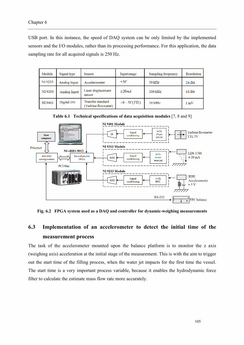
Chapter 6
105
USB port. In this instance, the speed of DAQ system can be only limited by the implemented
sensors and the I/O modules, rather than its processing performance. For this application, the data
sampling rate for all acquired signals is 250 Hz.
Table 6.1 Technical specifications of data acquisition modules [7, 8 and 9]
Fig. 6.2 FPGA system used as a DAQ and controller for dynamic-weighing measurements
6.3 Implementation of an accelerometer to detect the initial time of the
measurement processThe task of the accelerometer mounted upon the balance platform is to monitor the z axis
(weighing axis) acceleration at the initial stage of the measurement. This is with the aim to trigger
out the start time of the filling process, when the water jet impacts for the first time the vessel.
The start time is a very important process variable, because it enables the hydrodynamic force
filter to calculate the estimate mass flow rate more accurately.
Chapter 6
106
This technique is based on the physical fact that the incoming water jet will generate an impact
on the balance platform, and eventually, the weighing system will have to react mechanically to
such an impulse force in terms of a sudden acceleration [10].
If the weighing system output response were used instead, as the basis to trigger out the start time
of the measurement process, then the estimate measurand values would take longer to stabilize.
The explanation to this phenomenon lie on an smaller time constant and higher data sampling
frequency of the accelerometer, in relation to its counterpart, the weighing system.
As a matter of definition, the difference in time between the EFC balance response and the
acceleration response to the first water jet impact will be denoted as time offset. In Section 6.5, an
experimental test exemplifies the magnitude of such a time offset effect.
The employed Brüel & Kjaer 4508 DeltaTron® accelerometer is a compact (1cm3), hermetic, and
a light-weight (4,8 g) piezoelectric transducer. One of the remarkable features of this
accelerometer is its low noise pre-amplifier [11] incorporated in the transducer, as well as the
low-impedance cable used to prevent erroneous measurements due to voltage drops. The
transducer is connected to a 4-Channel NI 9233 module [7], which is dedicated to serve as a
power supply, A/D converter, amplifier, and digital filter for the accelerometer output signal.
Concerning its mounting, the accelerometer and its cable have to be properly fastened to the
weighing platform in order to avoid measurement errors caused by the wiggle of the sensor and
the triboelectric noise induced by the cable movement [12 & 13]. According to the PTB
acceleration laboratory, the measurement uncertainty of this accelerometer is in the order of
±0,2% at a confidence level of 95%.

Chapter 6
107
6.4 Usage of a non-contact laser displacement sensor to characterize the
water jet impact heightThe Micro-Epsilon NCDT 1710 Laser Displacement Sensor (LDS) is a measurement device
responsible of determining the water jet impact height ih z , which is a key process variable for
the experimental estimation of mass flow rate via hydrodynamic force filter.
As shown in Fig. 6.3, the LDS is mounted over the weighing system platform to monitor its
oscillatory displacement with a resolution of 0,5 µm, at a data sampling frequency of 250 Hz, and
a measurement uncertainty of 2µm (95% confidence level). This device working under the
triangulation measurement principle [14 and 15] is an appropriate sensor for this application,
because it does not exert any undesired additional force upon the balance platform.
The characterization of the impact height ih z was determined by filling the collection vessel at
10 different levels, measuring the corresponding distance between the nozzle outlet and the water
surface, and recording the displacement of the calibrated balance at each level by using the LDS.
Afterwards, these two variables are plotted to yield a characterization curve depicted by Fig. 6.3.
Thus, the current water jet impact height is a function of the balance displacement (z), wherein its
trend can be approximated by a quadratic curve-fitting equation, Eq. 6.5. The range of the water
jet impact height is between 520 mm (distance from nozzle outlet to vessel bottom) and 250 mm
(distance from nozzle outlet to the water surface at 10 L of the vessel capacity). As a remark, the
non-linear representation of Eq. 6.5 is due to the side wall shape of the vessel at the bottom.
2ih (z)= -1339 z - 863,09 z+515,82 (6.5)

Chapter 6
108
Fig. 6.3 Water jet impact height characterization as a function of the EFC balance platform
displacement measured by the LDS
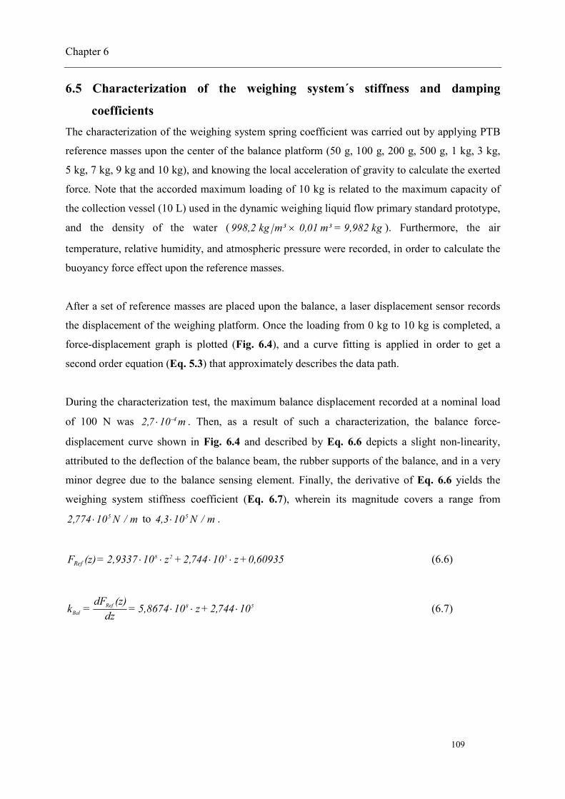
Chapter 6
109
6.5 Characterization of the weighing system´s stiffness and damping
coefficientsThe characterization of the weighing system spring coefficient was carried out by applying PTB
reference masses upon the center of the balance platform (50 g, 100 g, 200 g, 500 g, 1 kg, 3 kg,
5 kg, 7 kg, 9 kg and 10 kg), and knowing the local acceleration of gravity to calculate the exerted
force. Note that the accorded maximum loading of 10 kg is related to the maximum capacity of
the collection vessel (10 L) used in the dynamic weighing liquid flow primary standard prototype,
and the density of the water ( 998,2 kg m³ 0,01 m³ = 9,982 kg ). Furthermore, the air
temperature, relative humidity, and atmospheric pressure were recorded, in order to calculate the
buoyancy force effect upon the reference masses.
After a set of reference masses are placed upon the balance, a laser displacement sensor records
the displacement of the weighing platform. Once the loading from 0 kg to 10 kg is completed, a
force-displacement graph is plotted (Fig. 6.4), and a curve fitting is applied in order to get a
second order equation (Eq. 5.3) that approximately describes the data path.
During the characterization test, the maximum balance displacement recorded at a nominal load
of 100 N was -42,7 10 m . Then, as a result of such a characterization, the balance force-
displacement curve shown in Fig. 6.4 and described by Eq. 6.6 depicts a slight non-linearity,
attributed to the deflection of the balance beam, the rubber supports of the balance, and in a very
minor degree due to the balance sensing element. Finally, the derivative of Eq. 6.6 yields the
weighing system stiffness coefficient (Eq. 6.7), wherein its magnitude covers a range from52,774 10 N / m to 54,3 10 N / m .
8 2 5RefF (z)= 2,9337 10 z +2,744 10 z +0,60935 (6.6)
Ref 8 5Bal
dF (z)k = = 5,8674 10 z+ 2,744 10dz (6.7)

Chapter 6
110
Fig. 6.4 Characterization of the weighing system stiffness coefficient
The determination of the weighing system damping coefficient was calculated in accordance to
Eq. 6.8 (previously described in Chapter 3), wherein such a system parameter is a function of
the stiffness coefficient Balk , the total mass supported by the balance Tm (t) (Eq. 6.9), and the
characterized damped angular frequency of the balance along its weighing axis d T( m (t))
depicted in Fig. 5.4, Chapter 5. Thus, according to Fig. 6.5 the damping coefficient is within
0,12 N.s/m and 0,26 N.s/m.
2 2ˆ ˆ ˆBal
1 2
Bal T d T T= 2 k m (t) ( m (t)) m (t)c (t) - (6.8)
ˆ ˆT v p w HFm (t)= m +m +m (0)+m (t) (6.9)

Chapter 6
111
Fig. 6.5 Characterization of the weighing system damping coefficient (Eq. 6.8)
6.6 ResultsA very important stage during this research was to validate the process model used to determine
mass flow rate via dynamic-weighing. This task consisted in getting the results delivered by the
transfer standard (turbine flowmeter), and thereafter comparing such reference measurements
with the proposed approach. The set of experimental tests described in the following parragraphs
below, correspond to two stages carried out in order to obtain the measurand mass flow rate
(see Fig. 6.6).
1. Mass flow rate determination by means of an algorithm (Hydrodynamic force filter), which
takes as an input the acquired signal from the balance force response and time, and it is
responsible of quantifying and minimizing the effects from the hydrodynamic and buoyancy
force from the measurement,
2. A subsequent filter algorithm called Measurement noise filter, uses the outcome from the
Hydrodynamic force filter as an input signal, and deals with the attenuation of the
measurement noise caused by the dynamic response of the weighing system. In this analysis,
there are three different measurement noise filters proposed for this task (Moving average,
Least-mean-Square adaptive, and a Kalman filter), with the aim to compare their ability to get
rid of such a signal disturbance, and thus, delivering a more accurate estimate measurand.

Chapter 6
112
Fig. 6.6 Process model subsystem
6.6.1 Hydrodynamic force filter
In the measurement process, the hydrodynamic and buoyancy force have to be taken into account
in order to avoid a significant systematic error in the determination of mass flow rate via dynamic
weighing. With regard to the buoyancy force, this can be estimated by knowing the temperature-
dependent density from the air and water. On other hand, the hydrodynamic force induces a
larger undesired force magnitude to the measurement process caused by the time-varying force of
the water jet impacting the collection vessel. Fig. 6.7 describes an experimental test to prove the
influence of this variable, and to estimate its force magnitude. The experiment consisted of
starting the water collection process, and then bypassing the water jet from the collection vessel.
The result is a difference in force magnitude between the fluid in motion (collected mass force +
hydrodynamic force – buoyancy force), and the fluid at rest (collected mass force – buoyancy
force), which concludes in an estimated hydrodynamic force [16].
Fig. 6.7 exemplifies such an estimate at a nominal mass flow rate of 8 kg/min. In this instance,
the value of the hydrodynamic force at the initial stage of the filling process is 0,51 N, that
decreases to 0,4 N (or 20 %) at the final stage of the collection, because of the reduction of the
water jet impact height.

Chapter 6
113
Fig. 6.7 Experimental estimation of the hydrodynamic force at 8 kg/min

Chapter 6
114
6.6.2 Analytical and experimental estimation of the hydrodynamic force
The same type of experiment depicted in Fig. 6.7 was performed at 3 kg/min, 5 kg/min and
8 kg/min but additionally, the hydrodynamic force was quantified by Eq. 6.10 (Chapter 4,
Eq. 4.15) and Eq. 6.11, with the aim to compare the agreement between the experimental and
analytical approach. The results shown in Fig. 6.8, reveal that most of experimental measuring
points at five different levels of collection, overlap with the values obtained by analytical means.
The largest deviations between these two approaches to estimate the variable were: 1,7% at
3 kg/min, 1,4% at 5 kg/min, and 1,5% at 8 kg/min.
2
( )
( )( )
( )
( )
ˆ ˆ ˆ
ˆ
A
ww
A
w
AHF n HF n
w
ABal n n HF n Bal n
w
24 2 2 2
i n2 2w n
1 m (t )+ 2 g h (z) g 1- t m (t )+...ρ A
...+ 2 F (t ) g 1- t m (t ) F (t )=0
(6.10)
2ˆˆ ˆˆ ( ) ( )
1 / 2
HF nd n HF n
ww ni
m (t )F (t )=m t +2 g h (z)A
(6.11)
wherein the estimate water jet impact height ih (z) can be calculated by Eq. 6.5.
It is important to remark that the data scattering yield by the analytical form is highly spread
during the first seconds of the process due to the balance reacting shock response. Nonetheless,
such data spread (originated by the oscillatory response of the balance) does significantly
decrease as the collected water level rises.

Chapter 6
115
Fig. 6.8 Analytical and experimental estimation of the hydrodynamic force at 8, 5 and 3 kg/min
6.6.3 Estimation of the collected mass force
The estimation of the collected mass force is a key step for determining how good the
measurement process model will approach to the real water mass collection, and subsequently the
mass flow rate. The experimental results illustrated in Fig. 6.9 show the balance force response at
8 kg/min. This signal, as previously demonstrated in Fig. 6.8, contains the undesired magnitude
of the hydrodynamic and buoyancy force. Therefore, the task of the hydrodynamic force filter is
to significantly reduce these dynamic process variables, thus yielding an estimate of the collected
water mass. The removal of these dynamic forces is clearly seen in Fig. 6.9 when comparing the
slope of the balance force response and the given by the hydrodynamic force filter algorithm. As
expected, the slopes are different because the attenuated dynamic variables vary in time. As
observed in Fig. 6.9, the slope percent change of the hydrodynamic force filter output signal with
respect to Balance output response (Non-treated process signal) at three different mass flow rates,
were in the order of: 0,35 % at 8 kg/min, 0,28% at 5 kg/min, and 0,20% at 3 kg/min. The results
here infer that the balance force response trends to converge the estimate collected mass force,
Chapter 6
116
either at the lowest flow rates or at high levels of the collection process, associated with the
shortened water jet impact height. Moreover, this outcome suggests a worthwhile design criterion
of reducing as much as possible the distance from the discharging nozzle to the collection vessel
bottom, with the goal to physically decrease the hydrodynamic force magnitude from the
measurement process.
It is appropriate to highlight the term slope in this analysis, because in this measurement process
the slope implies a mass flow rate calculation. Fig. 6.10 clearly highlights the difference when
the balance force response and hydrodynamic force filter output as quotients of time (mass flow
rate). Note that the local acceleration of gravity 9,8125 m/s² [17] has been employed in order to
present the data as an estimate of kg/min. The estimate mass flow rate obtained by the direct
quotient of the balance output and time reveals a relative error of about 0,2 % in relation to the
average reference value given by the transfer standard (Fig. 6.10).
On the other hand, a smaller relative error of 0,07% is attained by using the estimate collected
water mass (Hydrodynamic force filter) to calculate the flow unit. After analyzing the tests at 3,
5, and 8 kg/min, it was concluded that the filter enable the measurements to improve by a factor
between 2 and 3.
Fig. 6.9 Hydrodynamic force filter used to estimate the collected water mass at 8 kg/min

Chapter 6
117
Fig. 6.10 Comparison of the average mass flow rate measurements via hydrodynamic force filter
and balance output signal
As a remark, the scattered data seen in Fig. 6.10 (caused largely by the time-discrete oscillatory
response of the balance) will be treated by the following filter algorithm (see Fig. 6.6), which
tackles the attenuation of the measurement noise.
6.6.4 Time offset correction
The experimental results shown in Fig. 6.10 were possible because the data was corrected from
the time offset originated by the balance response (Section 6.4.2). Such a correction enables the
measurement process to recognize at which point the collection process indeed started, so then an
initial time (or time zero) can be set for the calculations of mass flow rate. As previously
discussed in Section 6.4.2, this technique works under the principle of sudden acceleration of the
weighing system caused by the first impact of the water jet impacts upon the collection vessel.
An example of this method is illustrated in Fig. 6.11, wherein an accelerometer mounted upon
the weighing axis (perpendicular axis to the balance platform) measures the right moment of the
impact at 2,616s instead of at 2,661s given by the balance readout. This means, 45 ms faster than
the first step of the balance output response. The observed time delay between the two systems is
will depend upon the accelerometer time constant, the internal filter of the balance, and the higher

Chapter 6
118
sampling frequency of the accelerometer DAQ module (250 Hz), in relation to a 25-Hz data
sampling frequency from the EFC balance.
In order to exemplify the relevance of this parameter, consider the first step response of the
balance output signal as a reference mark for the process initial time. In this circumstance, the
calculation of the estimated mass flow rate depicted in Fig. 6.12 (with no time-offset correction),
would nearly require half of its measurement time (29 s) in order to converge with the average
reference value. The latter value agrees within an error band of 0,3% at 8 kg/min. On the other
hand, the other two mass flow rates at 5 kg/min and 3 kg/min, depict an stabilization time at
approximately 40% and 28% of their total measurement time, respectively. These numbers
demonstrate that the time offset significantly affects the high mass flow rates, due to the relative
short time of collection to compensate the weighing system time delay. As for the time-offset
corrected signal, this would require about 2s to get stable (Fig. 6.12). Therefore, almost the entire
set of data can be worth for analyzing.
Fig. 6.11 Determination of the filling process initial time based on the sudden acceleration of
weighing system when the water jet impacts for the first time

Chapter 6
119
Fig. 6.12 Time-offset effect upon the hydrodynamic force filter´s mass flow rate estimate values
Fig. 6.13 summarizes the three mass flow rates performed in this experiment with sets of three
measurement points each. The aim of gathering this information is to observe how relevant is the
minimization of the hydrodynamic force as well as the buoyancy force for the accuracy
enhancement of the measurand. Below, there are some remarks extracted from these data.
At 8 kg/min, the mass flow rate values given by the balance readout are out of the ± 0,09%
uncertainty level of the transfer standard. Furthermore, the relative error yield by the
hydrodynamic force filter is nearly in the limit of the uncertainty value of the transfer standard.
However, when comparing the two calculation approaches: the Balance response ˆ ( )Bal nm t
(Eq. 4.1) and the hydrodynamic force filter ˆ ( )HF nm t , it is clear that the hydrodynamic force filter
has improved the measurement accuracy by a factor of 2.
The measurements taken from both measuring methods at 5 kg/min show closeness to the
reference value, within ±0,06% and ±0,025% for the balance readout and hydrodynamic force
filter, respectively. At 3 kg/min, both measurement approaches were also within the claimed
uncertainty level of ±0,1%,. However, the percent relative error between 0,02% and 0,05%
turned out to be a bit larger than expected, when compared with the previous higher flow rate at
5 kg/min (narrow range between 0,02% to 0,025%).

Chapter 6
120
Fig. 6.13 Measurement comparison of estimate mass flow rates by means of using a hydrodynamic
force filter and by direct balance output response

Chapter 6
121
The fluctuating mass flow rate can be another contributing factor in the average relative error
shown in Fig. 6.13, and particularly at 3 and 5 kg/min. This assumption can be explained by
when comparing the possible correlation existing between the average percent relative error
(Fig. 6.14), and the approximated level of fluid flow fluctuation measured by the transfer
standard (Fig. 6.14). Here, the highest data dispersion is found in both cases at the lowest and
highest flow rate (3 kg/min and 8 kg/min), and the smallest at the mid flow rate, 5 kg/min.
Fig. 6.14 Quasi-steady mass flow rate data measured by the transfer standard
The term average relative error is highlighted with the intention of illustrating how the estimate
fluctuating mass flow rate depicted in Fig. 6.14 can impact the measurand value of the transfer
standard or a flowmeter. This situation is present in a major or a minor degree, even if the
measurement process is intended to be carried out at a constant mass flow rate (an ideal condition
that cannot be achieved so far by any liquid flow calibration facility). These observations are
important to be kept in mind, especially in a static weighing system, which is unable to monitor
this non-steady parameter, and its implications in terms of the measurement accuracy of the
flowmeter under calibration.

Chapter 6
122
6.6.5 Summary
Fig. 6.15 presents the results of the different approaches used to estimate the time-varying mass
flow rate in the form of a histogram. Such approaches are listed below, in accordance to the block
diagram of the process model subsystem shown in Fig. 6.6.
1. Balance force response (Eq. 4.1),
2. Hydrodynamic force filter,
3. Three proposed measurement noise filters:
a) Central moving average,
b) Least-Mean-Square (LMS) adaptive filter, and
c) Linear Kalman filter,
4. Flowmeter used as a transfer standard (measurand reference)
For instance, in Fig. 6.15 the balance force response and the hydrodynamic force filter
approaches feature equally wide data distribution, which is due to the fact that both signals have
not been treated at this point by the influence of the measurement noise. As recalled, the
measurement noise is referred as the noisy signal embedded in the balance output response, and it
is considered to be mostly caused (but not entirely) by the dynamics of the weighing system, in
response to the existing measurement process fluid-mechanical conditions. On the other hand, the
difference seen between these two approaches is indeed in terms of their mean value, which in
case of the hydrodynamic force filter turns out to be closer to the reference mean value, because
its data have been corrected from the water jet impact force and the air buoyancy effects upon the
measurand. At the first glance, Fig. 6.15 could suggest that the percent relative difference
between the hydrodynamic force filter and the transfer standard mean values is proportional to
the operational mass flow rate. However, when looking more carefully at the percent relative
difference of the hydrodynamic force filter data at 5 kg/min (0,018%), it turns out to be smaller
than at 3 kg/min (0,03%), and therefore, it implies that such a statement cannot be simply taken
for granted.
One of the possible explanations about why this relative difference magnitude is not fully (or
necessarily) proportional to the mass flow rate can be related with the level of flow steadiness
and its stationary condition. For example, the measurements carried out at 3 kg/min and 8 kg/min
feature a multi-peak histogram, meaning that such mass flow rate data were not only quasi-steady

Chapter 6
123
in the process, but also slightly shifting (decreasing) from its nominal mean value (Fig. 6.14). In
this case, the given conditions imply that the largest peak in the data distribution corresponds to
the flow rate that lasted longer during the measuring run, and whereby its mean value will trend
to lie in that direction (out of the range midpoint as seen in Fig. 6.15). On the other, when looking
at the measurement data at 5 kg/min, one can be inferred that a more steady and stationary flow is
taking place, because the transfer standard reference data depict a more homogeneous
distribution.
As for the LMS adaptive filter performance, it is observed that besides attenuating the induced
measurement noise (compared to the hydrodynamic force filter), it turns out its mean value nearly
coincides with the mean value of the central moving average filter, as shown in Fig. 6.15. One
reason for this common behavior is that for this specific data processing task, both filter
algorithms obtained a similar weighted average magnitude (with their corresponding coefficients)
for the three selected mass flow rates.
Concerning the central moving average, it is demonstrated in Fig. 6.15 that despite its limited
number of estimate values, (in relation to its counterparts, LMS adaptive and Linear Kalman
filters), it is able to deliver precise and accurate results. The latter statement applies even if the
mean value of the central moving average was not overlapping the reference data at 8 kg/min
(with a relative difference of 0,09%). This is because, in practice, the true mass flow mean value
can lie within the claimed uncertainty of ±0,1%, in relation to the transfer standard mean value.
On the other hand, as already recalled in Chapter 5, the number of estimate values (17 at
8 kg/min, 22 at 5 kg/min, and 47 at 3 kg/min) given by the central moving average should not be
a limitation, because 5 to 10 measurements per mass flow rate can be statistically sufficient to
calibrate a flowmeter.

Chapter 6
124
Fig. 6.15 Histograms summarizing the different mass flow rate estimation processes
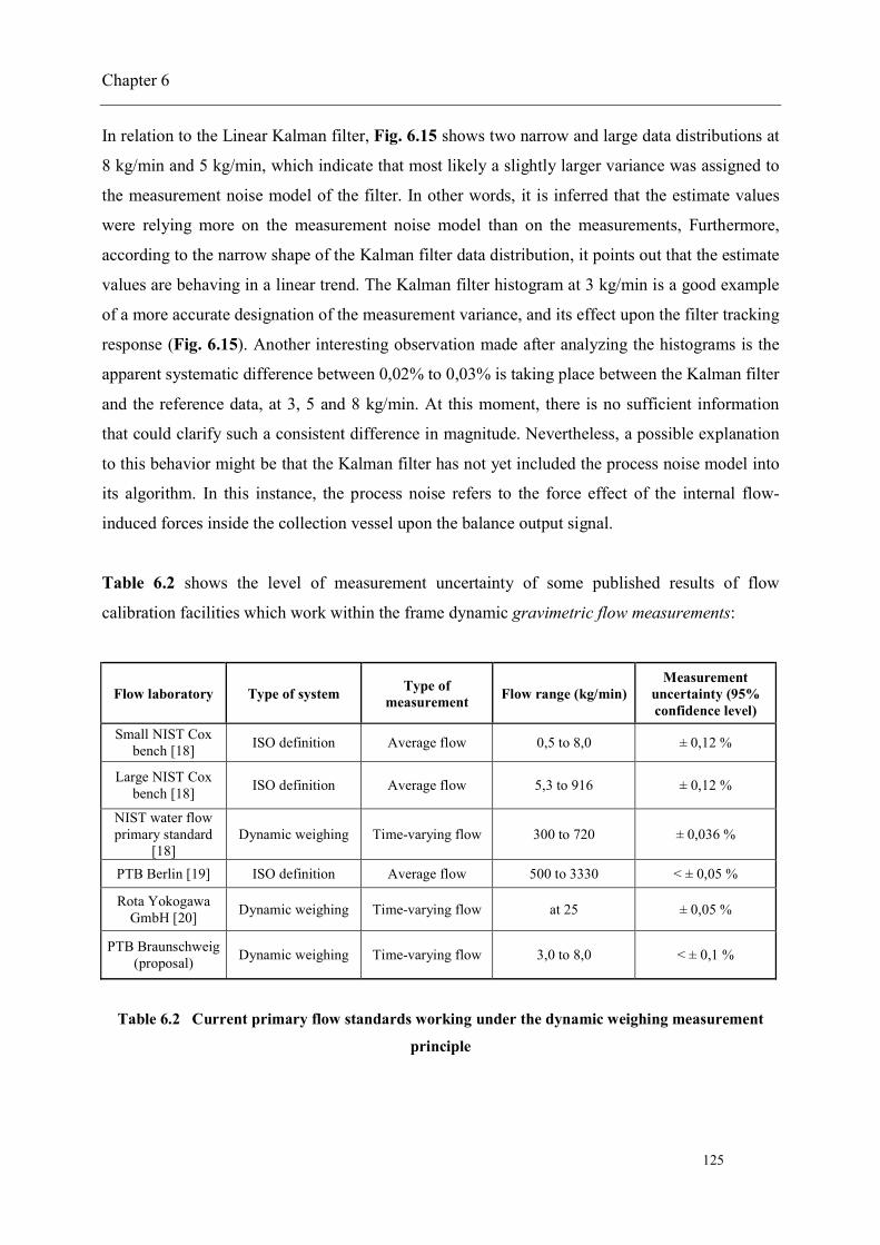
Chapter 6
125
In relation to the Linear Kalman filter, Fig. 6.15 shows two narrow and large data distributions at
8 kg/min and 5 kg/min, which indicate that most likely a slightly larger variance was assigned to
the measurement noise model of the filter. In other words, it is inferred that the estimate values
were relying more on the measurement noise model than on the measurements, Furthermore,
according to the narrow shape of the Kalman filter data distribution, it points out that the estimate
values are behaving in a linear trend. The Kalman filter histogram at 3 kg/min is a good example
of a more accurate designation of the measurement variance, and its effect upon the filter tracking
response (Fig. 6.15). Another interesting observation made after analyzing the histograms is the
apparent systematic difference between 0,02% to 0,03% is taking place between the Kalman filter
and the reference data, at 3, 5 and 8 kg/min. At this moment, there is no sufficient information
that could clarify such a consistent difference in magnitude. Nevertheless, a possible explanation
to this behavior might be that the Kalman filter has not yet included the process noise model into
its algorithm. In this instance, the process noise refers to the force effect of the internal flow-
induced forces inside the collection vessel upon the balance output signal.
Table 6.2 shows the level of measurement uncertainty of some published results of flow
calibration facilities which work within the frame dynamic gravimetric flow measurements:
Flow laboratory Type of system Type ofmeasurement Flow range (kg/min)
Measurementuncertainty (95%confidence level)
Small NIST Coxbench [18] ISO definition Average flow 0,5 to 8,0 ± 0,12 %
Large NIST Coxbench [18] ISO definition Average flow 5,3 to 916 ± 0,12 %
NIST water flowprimary standard
[18]Dynamic weighing Time-varying flow 300 to 720 ± 0,036 %
PTB Berlin [19] ISO definition Average flow 500 to 3330 < ± 0,05 %
Rota YokogawaGmbH [20] Dynamic weighing Time-varying flow at 25 ± 0,05 %
PTB Braunschweig(proposal) Dynamic weighing Time-varying flow 3,0 to 8,0 < ± 0,1 %
Table 6.2 Current primary flow standards working under the dynamic weighing measurement
principle

Chapter 7
126
7. Conclusions and outlook
In this research work, a new method for the calibration of liquid flowmeters was presented, for its
future application in liquid flow calibration laboratories. The characteristics, advantages and
limitations of this new method have been described in terms of its principle of functionality as
well as the next steps to be taken, in order to improve its current performance. This chapter
summarizes all the conclusions and remarks of this ongoing long-term investigation.
First, it was necessary and feasible to simulate the measurement process (Chapter 3), with the
aim to understand the system’s dynamic response, the main sources of noise in the process, their
source, the role and significance of different process variables, and to verify the consistency of
the experimental results. In this instance, the simulation applies to a 1 Degree-of-Freedom model,
which despite analyzing the normal weighing axis (z axis), it highlights the most striking fluid-
mechanical forces in the process: the water jet impact force, the collected mass force, the
buoyancy force acting upon the system normal axis, and the normal reacting force of the
weighing system
This calibration method can significantly reduce the calibration time, because it only requires a
single measuring run (one collection per calibration point), and at the same time is capable of
generating a large amount of measurement data for the characterization of a flowmeter. For ex-
ample, the factor of calibration time reduction could be agreed to be five, if one considers that
each calibration point (i.e. static weighing method) requires at least five measurements. This
number is based on some calibration procedures [1], which consider that amount of data as statis-
tically sufficient for a measurement uncertainty analysis (Section 1.2). Another advantage of this
calibration method is the possibility to implement it in a static weighing liquid flow primary
standard, without the necessity to modify the mechanical design of such a facility. This means
that the user can perform a flowmeter calibration, either in a static or in a dynamic weighing
mode by using a single facility. Moreover, in a dynamic weighing liquid flow primary standard,
the thorough characterization and fast actuation of a diverter valve (Chapter 2) is not longer a
system requisite, since the proposed calibration principle only requires the diverter valve to act as
an ordinary bypass valve, to directs the fluid into the vessel, and bypasses it back to a supply tank
when the collection is completed.

Chapter 7
127
In the hydrodynamic force filter, the effect and quantification of the water jet turbulence as well
as the viscous shear stress caused by the water jet-air interaction [2] were not included in the
current analysis, due to the complexity in deriving an analytical model. However, as
demonstrated in experimental tests, the simplified water jet impact force model (based on the
Bernoulli equation, geometry and dimensions of the system) proves to be good enough in
estimating the average impacting force of the water jet (Chapter 6). In this case, the average
impact force can be calculated, due to the fact that the turbulent flow is quasi-steady [3]. In
summary, even if such a force cannot be exactly quantified, it greatly helps in diminishing the
unwanted hydrodynamic force effect from the process. This is clearly seen in Chapter 5 and
Chapter 6, wherein such a filter is compared with a mass flow rate calculation that overlooks the
water jet impact force.
As for the three proposed measurement noise filters, the following observations were made. The
central moving filter yields a limited number of estimates in relation to the LMS adaptive and the
Kalman filter. Nevertheless, such a number can turn out to be sufficient and accurate enough, if
compared with the number of data samples required in a regular calibration procedure. In regards
to the LMS adaptive filter, it estimates the time-varying mass flow rate in a similar way the cen-
tral moving average does, except that the adaptive filter can reproduce more estimates than the
central moving average. On the other hand, in terms of their initial response, the LMS adaptive
filter and the central moving average require some time to converge the reference values, and to
overcome the high-amplitude overshoot response seen at the first 1/3 of the collection time. The
third proposed algorithm, the linear Kalman filter requires less computational power than the
LMS adaptive filter. Furthermore, as observed at the results in Chapter 5 and Chapter 6, the
Kalman filter seems to deal better with the high-amplitude measurement noise at the beginning of
the process, as well as tracking and estimating more effectively the fluctuating mass flow rate.
The usage of the average mass flow rate magnitude (obtained from the hydrodynamic force filter
data) turned out to be an appropriate estimation parameter for the Kalman filter and the LMS
adaptive filter because, as already mentioned, the process was carried out at quasi-steady flow
conditions. And, as demonstrated in numerical and experimental results, the Kalman filter deliv-
ers the largest number of estimates with the lowest percent of relative error. Therefore, it was
chosen as the measurement noise filter.

Chapter 7
128
As for the experimental tests, accuracy levels of less than ±0,1% are attainable by applying the
dynamic weighing liquid flow calibration approach. However, it is worth recalling that this
number is given in accordance to estimate mass flow rate values that stood within the claimed
accuracy of the PTB transfer standard (used in the comparison test). Another interesting
characteristic found in some experimental data was the similar time-varying mass flow rate
measured by the two different approaches (the process model and the transfer standard), which
suggests that in reality the flow might indeed follow such a particular path (Chapter 6).
Nonetheless, in order to confirm this observation, it is necessary to compare the proposed
calibration method with another high-accurate flow primary standard such as a piston prover
(Chapter 2) or a Laser Doppler Anemometer system (LDA) [4].
According to numerical tests, the accuracy and precision of the measurements could be signifi-
cantly enhanced if the data sampling frequency of the weighing system was increased, and the
low pass filter avoided. This also raises the conclusion that a customized balance for this particu-
lar application would be the ideal case, by allowing the user to acquire the balance analog output
signal without aliasing effects, understanding and treating more effectively the unwanted process
and measurement noisy signals from the acquired data, and thus, obtaining a more accurate mass
flow rate estimate. Furthermore, the concept of a customized balance would also help in the sense
of getting a closer numerical representation of the physical weighing system, in terms of studying
in depth the impact of the system dynamics upon the measurand determination (i.e. knowing the
algorithm of the balance positioning control loop).
According to the mechanical frequency analysis presented in Chapter 6, it is demonstrated that
the system is subjected to move not only along its weighing axis, but also to at least two
additional translational and/or rotational axes. From the previous observations made and in the
literature [5 and 6], it indicates that this behavior is caused by the acting radial fluid forces of a
generated vortex inside the collection vessel, and the reacting orthogonal forces of the balance
(due to the slight transverse sensitivity of its cell). To better understand this system condition and
its influence on the balance output signal (mechanical crosstalk effect), it is necessary to analyze,
in future, the system as a 2 or 3 Degrees-of-Freedom case. The process requires that the model
should include the time-varying acting moment (torque) generated by the normal and radial fluid
forces [7] and their location, and the reacting time-varying moment of inertia of the system
during its operation. In order to apply this concept, it is necessary to know (or to estimate) the

Chapter 7
129
magnitude of these acting forces. Therefore, it will be required to quantify their magnitudes by
using an experimental approach, such as the Particle Image Velocimetry (PIV) [8], and/or a
numerical analysis via Computational Fluid Dynamics (CFD) [5]. In terms of its application, this
process condition can be added into the Kalman filter; so that the algorithm will be able to take
into account some of the process noise generated by the fluid dynamics as well as the recalled
system measurement noise. This will benefit the calibration procedure in re-enhancing its current
accuracy and precision.
As a next step in this research work, the mechanisms for effective system´s energy dissipation [9]
have to be investigated. A liquid flow primary standard has to be designed in such a way that its
dimensional and geometrical characteristics (i.e. the vessel diameter and its height, the system´s
mass, the discharging nozzle cross section area, and its location), allow it to diminish the level of
disturbance caused by the stored kinetic energy in the system (The higher the rate of energy
dissipation, the lower the influence of the process and measurement noise upon the measurand).
In practical terms, this rate of energy dissipation can be correlated with the system´s inertial force
or its oscillatory acceleration.
The influence of the water surface waves in the collection vessel and the water jet mass have not
being treated in this research work. However, for the case of the water surface waves, this
phenomenon cannot be disregarded for a future analysis because, as visually observed, this is an
inherent process characteristic, which might influence (in some measure) the balance response [10].
On the other hand, it is more appropriate to first investigate the influence of the internal vortex
because this process variable, in addition to the water jet impact is responsible (cause) for
generating the surface waves (effect). Moreover, in accordance to the experiments carried out, the
influence of the water jet mass (interpreted as a water mass column) was not observed, as Shinder
et al. mention in its analysis [11]. However, this is not discarded, and it will be reconsidered in
future experiments, in order to ensure whether that variable takes place in the measurement
process or not.

Nomenclature
130
Nomenclature
A: Transition matrix
A: Arbitrary cross section area in a pipeline
CVA : Arbitrary area of the connecting volume wherein the mass flow passes through
MeterA : Cross section area of the flowmeter
nA : Cross section area o the nozzle outlet
PistonA : Inner cross section area of a piston prover
vA : Cross section area of the collection vessel
Balc (t) : Damping coefficient of a mechanical system
nE : Characteristic time-varying matrix
( )AF ne t : Feedback error signal estimate (Adaptive filter)
bF (t) : Time-varying buoyancy force
BalF (t) : Balance reacting force due to its stiffness coefficient
BalLPFF (t) : Time-varying oscillatory force response of the balance driven by the low pass
filter
cF (t) : Weighing system damping force
dF (t) : Time-varying hydrodynamic force caused by the water jet impact
InertialF (t) : Time-varying inertial force exerted by the weighing system
m(t)F : Fluid force due to time-varying collected mass and local acceleration of gravity
qF (t) : Additional fluid forced acting upon the weighing system (i.e. Vortex axial and
water wave oscillatory forces)
TF (t) : Time-varying total fluid force
Mech (t)F : Summation of weighing system mechanical forces
fd: Balance frequency response
LPFf : Low-pass filter cutoff frequency
Nomenclature
131
nMeterf t : Turbine flowmeter rotor frequency
LPF dG (f ) : Low pass filter gain factor
g: Local acceleration of gravityH : Measurement matrix
h(k) : Current k-number filter coefficient (Least-Mean Square adaptive filter)
ih (t) : Water jet impact height
ih (0) Initial water jet impact height
i nh (t ) : Discrete time-varying estimate of the water jet impact height
ih (z) : Water jet impact height estimate as a function of the balance displacement
uph k : Update k-number filter coefficient (Least-Mean Square adaptive filter)
wh (t) : Increasing height of the water surface
I: Identity matrix
nK : Kalman gain matrix
MeterK : Turbine flowmeter calibration factor
Balk : Balance stiffness coefficient
M: Number of filter coefficients
m(t) : Continuous time-varying estimate mass flow rate
ˆnBalm (t ) : Average discrete time-varying mass flow rate
ˆnHFm (t ) : Hydrodynamic force filter estimate of time-varying mass flow rate
ISOm . Reference mass used by an ISO dynamic gravimetric liquid flow primary standard
Km : Mean mass flow rate (Kalman filter)
K nm (t ) : Discrete time mass flow rate estimate (Kalman filter)
ˆ )MA nm (t : Discrete time-varying mass flow rate estimate via moving average filter
ˆ )+MA nm (t : A priori discrete time-varying mass flow rate estimate via moving average filter

Nomenclature
132
ˆ )-MA nm (t : A posteriori discrete time-varying mass flow rate estimate via moving average
filter
Meter nm ( t ) : Mass flow rate measured by the flowmeter
pm: Weighing platform mass
Totalm : Total fluid mass
Tm (t) : Continuous time-varying total mass held by the balance elastic elements
Tr1m : Reference-mass triggering point (Start) according to ISO dynamic gravimetric
liquid flow primary standard
Tr2m : Reference-mass triggering point (Stop) acc. to ISO dynamic gravimetric liquid
flow primary standard
vm : Collection vessel mass
wm : Mass flow rate
wm (t) : Continuous time-varying collected water mass
w nm (t ) : Discrete time-varying estimate mass flow rate
INwm : Mass flow rate of a fluid entering a finite volume
OUTwm : Mass flow rate of a fluid entering a finite volume
AFN : Number of input signal data
NMA: Number of data samples used by the moving average filter-nP : Predicted estimate error covariance matrix
AFP : Average power of the input signal data set (Adaptive filter)
p( ) : Eigenvalue polynomial equationR : Measurement noise covariance
ISOt : Collection time according to ISO dynamic gravimetric liquid flow primary
standard
tn: Discrete time
Pistont : Piston stroke time
Totalt : Total collection time

Nomenclature
133
neU t : Measurement uncertainty related to time-varying process model algorithm
CVU : Measurement uncertainty attributed to the connecting volume
u : Average fluid velocity at an arbitrary point
u( t ) : Mean velocity of the fluid at an arbitrary region across the connecting volume
Meteru ( t ) : Mean normal velocity at the flowmeter location
iu (t) : Normal impact velocity of the water jet
nu ( t ) : Mean normal velocity at the nozzle location
CVV : Connecting volume between weighing system and meter under calibration
PTBV : Volumetric flow rate determined by the PTB primary flow standard
TotalV : Total fluid volume
wV (t) : Time-varying collected water volume
nv(t ) : Discrete time-varying measurement noise estimate
nv(t )ˆ : Discrete time estimate measurement noise
( )K nv t : Discrete time measurement noise (Kalman filter)-nx : Current mass flow rate estimate vector
nx : Corrected state estimate value
Pistonx : Piston displacement
Pistonx : Piston velocity
ny : Current measurement vector
z: Balance normal displacementz : Weighing system velocity
z : Weighing system acceleration
Aρ : Air density
wρ : Water density
w_CVρ : Water density in the connecting volume
w_Meterρ : Water density at the flowmeter location

Nomenclature
134
w_nρ : Water density at the nozzle outlet
A Air temperature
w : Water temperature
d : Damped angular frequency of the balance
LPFω : Low-pass filter cutoff angular frequency
n (t) : Time-varying system´s natural angular frequency
LPF t : Low pass filter phase shift2K : Mass flow rate variance (Kalman filter)
wβ : Volumetric thermal expansion coefficient of water
CVα : Linear expansion coefficient of the connecting pipe
n(t ) : Discrete time-varying eigenvalues
Δ AF : Adaptive filter step size : Critical damping fraction
Acronyms
ISO: Internation Standardisation Organisation
PTB: Physikalisch-Technische Bundesanstalt
NIST: National Institute of Standards and Technology
MUC: Meter Under Calibration
CV: Connecting Volume
LPF: Low Pass Filter
EFC: Electromagnetic Force Compensation
LMS: Least-Mean Square algorithm
MA: Moving Average filter
NLMS: Normal Least-Mean Square filter
HF: Hydrodynamic Filter
DWLFS: Dynamic Weighing Liquid Flow Standard

References
135
References
Chapter 1[1] M. Rinker, G. Wendt, Legal Metrology in the Field of Fluid Measurement Technology,
PTB-Mitteilungen 119 (2009), No. 1, Special Issue “Metering Energy and Fluid Flows”,
Braunschweig, Germany, 2009, pp. 28-30
Chapter 2[1] O. Madsen, Summary of finite control volume analysis in fluid mechanics, Engineering
mechanics II, Faculty of civil and environmental engineering, Massachusetts Institute of
Technology (MIT), USA, April, 2006
[2] The Instrumentation, Systems and Automation society (ISA), The automation, systems
and instrumentation dictionary, Fourth edition, ISA, NC, USA, November, 2005
[3] M. Reader-Harris, J. McNaught, Impulse lines for differential pressure flowmeters: Best
practice guide, National Engineering Laboratory (NEL), Glasgow, UK, September, 2005
[4] J. Bentley, Principles of measurement systems, Fourth edition, Pearson education limited,
England, 2005
[5] D. Spitzer, Flow measurement: practical guides for measurement and control, Second
edition, The Instrumentation, Systems and Automation Society, ISA, USA, 2001
[6] R. Arias, Measurement uncertainty of an orifice plate flowmeter (In Spanish), National
center of metrology (CENAM), Querétaro, México, April, 2001
[7] R. Baker, Flow measurement handbook: Industrial designs, operating principles,
performance, and applications, Cambridge University press, USA, 2000
[8] R. Miller, Flow measurement handbook, Third edition, McGraw Hill professional, New
York, NY, USA, March, 1996
[9] S. Phillips, W. Estler, T. Doiron, K. Eberhardt, M. Levenson, A careful consideration of
the calibration concept, Journal of research of the National Institute of Standards and
Technology, NIST, Vol. 106, No. 2, Gaithersburg, MD, USA, April, 2001

References
136
[10] Bureau International des Poids et Mesures (BIPM), Concept of traceability and standards,
BIPM, Cedex, France, 2004, http://www.bipm.org/en/convention/wmd/2004/
[11] P. Espina, A question of accuracy: What does it mean to be traceable?, NIST,
Gaithersburg, MD, USA, 2000
[12] Bureau International des Poids et Mesures (BIPM), International vocabulary of
metrology: Basic and General concepts and associated terms (VIM), BIPM, Cedex,
France, 2008
[13] G. Wendt, R. Engel, J. Riedel, Ensuring the Traceability of Volume and Flow
Measurements of Liquids, PTB-Mitteilungen 119 (2009), No. 1,, Special Issue “Metering
Energy and Fluid Flows”, Braunschweig, Germany, pp. 23-27
[14] W. Pöschel, R. Engel, The concept of a new primary standard for liquid flow
measurement at PTB Braunschweig, The 9th International conference of flow
measurement, FLOMEKO 1998, Lund, Sweden, June 15th-17th, 1998
[15] A. Sleigh, C. Noakes, Fluid dynamics: The momentum and Bernoulli equations, CIVE
1400: Fluid Mechanics, Leeds University, UK, January, 2009
[16] R. Engel, B. Mickan, Aspects of traceability and comparisons in flow measurement, 7th
International Symposium on Fluid Flow Measurement (ISFFM), Alaska, USA, August
12th-14th, 2009
[17] W. Pöschel, R. Engel, D. Dopheide, H, Kecke, R. Praetor, N. Weist, E. Kurras, An unique
fluid diverter design for water flow calibration facilities, 10th International conference of
flow measurement, FLOMEKO 2000, Salvador, Brazil, June 5th-8th, 2000
[18] International Standard Organization, ISO 4185, Measurement of liquid flow in closed
conduits: Weighing method, First edition, Ref. No: ISO 4185-1980(E), Switzerland, 1980
[19] R. Paton, Calibration and standards in flow measurement, Reproduced from the
Handbook of measuring system design, John Wiley and Sons, Ltd, UK, 2005
[20] T. Yeh, J. Aguilera, J. Wright, NIST Hydrocarbon liquid flow calibration services,
Chemical science and technology laboratory, NIST special publication 250-1039, USA,
2005
[21] J. Kuttin, G. Bobovnik, I. Bajsic, Dynamic effects in a clearance-sealed piston prover for
gas flow measurements, Metrologia 48, UK, January 2011

References
137
[22] R. Arias, A. Loza, J. Lara, H. Luchsinger, Dynamic calibration of a bi-directional prover
for liquid flow measurements (In Spanish), National center of metrology (CENAM),
Internal publication, Querétaro, México, 2000
[23] M. van der Beek, Euroloop: Measurement concepts for efficient calibrations and primary
realization of accurate reference values in flow, FLOMEKO 2003, Groningen, The
Netherlands, 2003
[24] N. Mathies, Messunsicherheit einer gravimetrischen Kalt- und Warmwasser-
Normalmessanlage für große Volumenströme, Mensch und Buch Verlag, Berlin, 2005,
p. 85
[25] M. Shafer, F. Ruegg, Liquid-flowmeter calibration techniques, Transactions of ASME,
October, USA, 1958, p. 1369
[26] Küppers Elektromechanik GmbH, Durchflußmeßgeräte kalibrieren, Germany, 2010
[27] V. Ivashenko, K. Podkopaev, T. Taranenko, V. Skorobogatov, An automated standard
test system flow liquid flow rates, Translated from Izmeritel´naya Technika, No 4, Russia,
April, 1976, pp. 36-38
[28] R. Engel, Dynamic weighing – Improvements in gravimetric liquid flowmeter calibration,
The 5th International symposium on fluid flow measurement, Arlington, VA, USA, 2002
[29] X. Weilin, L. Huasheng, Y. Yongquan, W. Chigong, Turbulent flow and energy
dissipation in pluinge pool of a high arch dam, Journal of hydraulic research, Vol. 40,
No. 4, UK, December, 2002
[30] I. Shinder, I. Marfenko, NIST calibration services for water flowmeters, NIST special
publication 250, National Institute of Standards and Technology (NIST), Gaithersburg,
MD, August, 2006
[31] I. Shinder, M. Moldover, Accurately measuring unsteady water flows using a dynamic
standard, Measurement science conference, Annahein, CA, USA, March, 2009
[32] I. Shinder, M. Moldover, Dynamic gravitational standard for liquid flow: Model and
measurements, International symposium on fluid flow measurements, Alaska, USA,
August, 2009

References
138
Chapter 3[1] M. Kutz, Mechanical Engineers’ handbook, Instrumentation, systems, controls, and
MEMS, Third Edition, John Wiley & Sons, Inc., Hoboken, New Jersey, USA, 2006,
p. 387
[2] L. Brusquet, J. Oksman, Improving the accuracy of tracer flow measurement techniques
by using an inverse-problem approach, Measurement science and technology journal,
Vol. 10, UK, 1999, pp. 559-563
[3] I. Shames, Fluid Mechanics (Spanish),Third edition, McGraw Hill,USA,1995, p. 9
[4] M. Fogiel, The fluid mechanics and dynamics problem solver, Research and Education
Association (REA), New York, USA, 1984, p. 294
[5] Y.C. Fung, A first course in continuum mechanics, Prentice-Hall, Inc., Englewood Cliffs,
N.J., USA, 1969, p.13
[6] F. Jones, Techniques and topics in flow measurement, CRC Press, New York, USA, 2000,
p. 71
[7] R. Engel, Dynamic weighing – Improvements in gravimetric liquid flowmeter calibration,
The 5th International symposium on fluid flow measurement, Arlington, VA, USA, 2002
[8] A. Reichmuth, Measuring mass and force with a balance, Mettler Toledo, Vol.12,
Greifensee, Switzerland, June, 1999
[9] A. Reichmuth, Adverse influences and their prevention in weighing: Design and working
principles of laboratory balances, specifications of balances, and influences on balances
and weighing samples, Mettler Toledo, Vol. 13, Greifensee, Switzerland, May, 2001
[10] U. Berli, M. Bönzli, Electronic weighing principles, Mettler Toledo, Greifensee,
Switzerland, May, 1991
[11] E. Manske, T. Fröhlich, R. Füßl, Lehrmaterial zur Vorlesung Mess- und Sensortechnik,
Technische Universität Ilmenau, Fakultät für Maschinenbau, Institut für Prozessmess- und
Sensortechnik, Ilmenau, Germany, December, 2010
[12] J. Hartog, Mechanics, First edition, McGraw Hill, New York, USA, 1948, p.175
[13] C. Harris, A. Piersol, Shock and vibration handbook, Fifth Edition, McGraw Hill, New
York, USA, 2002, pp. 2.1-2.5 and 10.2

References
139
[14] D. Findeisen, System dynamics and mechanical vibrations, Springer-Verlag, Heidelberg,
Germany, 2000, p.30
[15] S. Timoshenko, H. Young, Engineering Mechanics, Third edition, McGraw Hill, New
York, USA, 1951, p. 303
[16] F. Axisa, J. Antunes, Modelling of mechanical systems: fluid structure interaction,
Volume 3, First edition, Elsevier Ltd., Oxford, Great Britain, 2007, p. 51
[17] BIPM, International vocabulary of metrology (VIM), France, 2008, p. 29
[18] P. Gaydecki, Foundation of digital design processing: Theory algorithms and hardware
design, IEEE, UK, 2004, p. 120
[19] Thomson Delmar Learning, Circuit analysis with devices: Theory and practice, Chapter
22, 2007, p. 19
[20] J. Wright, G. Mattingly, NIST Calibration services for gas flow meters, NIST Special
publication 250-49, NIST, MD, USA, August, 1998, p. 3
[21] D. Tritton, Physical fluid dynamics, Van Nostrand Reinhold (UK) Co, Ltd., Molly Millars
Lane, Wokingham, Berkshire, England, 1982, p. 45
[22] Y.C. Fung, A first course in continuum mechanics, Prentice-Hall, Inc., Englewood Cliffs,
N.J., USA, 1969, p.11
[23] T.T. Yeh, P. Espina, G. Mattingly, J. Aguilera, An uncertainty analysis of a NIST
hydrocarbon liquid flow calibration facility, Proceedings of ASME HT/FED 04, 2004
Heat transfer/ Fluids engineering summer conference, Charlotte, N.C., USA, July, 2004
[24] G. Elert, The physics hypertextbook: Thermal expansion, http://physics.info/expansion/,
USA, 2010
[25] M. Tanaka, R. Davis, A. Peuto, N. Bignell, Recommended table for the density of water
between 0 °C and 40 °C based on recent experimental reports, Metrologia, Vol. 38,
Issue 4, August, 2001
[26] EURAMET, Calibration of temperature block calibrators, EURAMET Technical
committee for thermometry, European Association of National metrology Institutes,
EURAMET/cg-13/v.01, July, 2007, p. 10

References
140
[27] R. Engel, H. Baade, Model-based flow diverter analysis for an improved uncertainty
determination in liquid flow calibration facilities, Measurement science and technology,
Volume:21, IOP Publishing, Ltd., UK, January, 2010
Chapter 4[1] W. Schmid, R. Arias, Estimation of measurement uncertainty (Spanish), National center
of metrology (CENAM), Querétaro, México, 2005, p.15
[2] R. Davis, A primer for mass metrology, NBS special publication 700-1, Industrial
measurement series, Gaithersburg, MD, USA, 1984, p. 8
[3] A. Coehlo, Signal processing and data filtering, University of Santa Catarina (UFSC),
Brazil, May, 2005, p.1
[4] A. Prasad, Introduction to error analysis, Dept. of Mechanical engineering, Univ. of
Delaware, USA, 2006, p.1
[5] H. Fryer, Concepts and methods of experimental statistics, Allyn and Bacon, Inc. Boston,
USA, 1966, p.4
[6] P. Sydenham, Static and dynamic characteristics of instrumentation, CRC Press,
University of South Australia, 2000, Section 3.2
[7] M. Gläser, M. Borys, Precision mass measurements, Reports on progress in physics,
No. 72, IOP Publishing, UK, 2009
[8] L. Yao, Linear and quadratic equation, Chapter 1, Math 10, University of North Carolina,
USA, 2005
[9] S. Goode, An introduction to differential equations and linear algebra, Prentice Hall,
New Jersey, USA, 1991, p. 283
[10] C. Moler, Numerical computing with MatLab®, Chapter 10,The MathWorks, Inc, Natick,
MA, USA, p. 17
[11] D. Lay, Linear algebra and its applications, Second edition, Addison-Wesley,
Massachusetts, USA, 2000, p. 311

References
141
[12] J. Aguilera, T. Yeh, J. Wright, Inside diameter measurements for the cylinder of a 20 L
piston prover, 6th International symposium on fluid flow measurement (ISFFM),
Querétaro, México, May 16th-18th, 2006
[13] NIST Statistical engineering division, Engineering statistics handbook, NIST, Maryland,
USA, June, 2010, Section 6.4
[14] A. Gelb, Applied optimal estimation, The Analytic Science Corporation (TASC), MIT
Press, Cambridge, MA, USA, 1974, pp. 23, 102-119, 156
[15] V. Stewart, Echo cancelling, Chapter 4, The Queen´s University of Belfast, Ireland, 2000,
p.59
[16] P. Maybeck, Stochastic models, estimation, and control, Volume 1, Academic Press, Inc.,
New York, USA, 1979, pp. 5-15
[17] S. Smith, The scientist and engineering guide to digital signal processing, chapter 15,
California technical publications, California, USA, 2000, p. 278
[18] Y. Chou, Statistical analysis for business and economics, Elsevier science Ltd.,
Amsterdam, The Netherlands, 1989, Section. 17.9
[19] D. Hyde, DPlot Graph software for scientist and engineers: Moving average, HydeSoft
Computing, Inc., Vicksburg, MS, USA, 2009
[20] M. Van Exter, Noise and signal processing, Chapter 2, University Leiden, The
Netherlands, August, 2003, p. 9
[21] P. Gaydecki, Foundation of digital design processing: Theory algorithms and hardware
design, IEEE, UK, 2004, pp. 120, 385-397
[22] C. Feldbauer, F. Pernkopf, Adaptive filters: A tutorial for the course in computational
intelligence, Institut für Grundlage der Informationverarbeitung, Technische Universität
Graz, Austria, June, 2010
[23] The MathWorks®, Inc., Filter design Toolbox 4: User´s Guide, chapter 5, MatLab®,
Natick, MA, September, 2010, pp. 5.20-5.24
[24] A. Poularikas, Z. Ramadan, Adaptive filtering primer with MatLab®, Taylor and Francis
Group, London, England, 2006, p. 2

References
142
[25] The MathWorks®, Inc., Filter design Toolbox 4: Getting started guide, Chapter 5,
MatLab®, Natick, MA, September, 2010, p. 5.4
[26] K. Rekha, B. Nagabushan, K. Nataraj, FPGA implementation of NLMS algorithm for
identification of Unknown systems, International journal of engineering science and
technology, Vol. 2 (11) 2010, Chennai, India, 2010, p. 6397
[27] National Instruments, Least Mean Square (LMS) algorithms (Adaptive filter toolkit),
Austin, TX, USA, June, 2008
[28] C. Toker, Recursive Least Squares (RLS) adaptive filters, Chapter 9, Department of
electrical and electronics engineering, Hacettepe University, Turkey, December, 2007
[29] M. Junnti, Communication signal processing: Recursive Least Squares (RLS) algorithm,
department of electrical and information engineering, University of Oulu, Finland,
February, 2008
[30] National Instruments, Recursive Least Squares (RLS) algorithms (Adaptive filter toolkit),
Austin, TX, USA, June, 2008
[31] R. Kalman, A new approach to linear filtering and prediction problems, transactions of
the ASME, Journal of basic engineering, 82 (series D), USA, 1960. pp. 35-45
[32] J. Mandel, The statistical analysis of experimental data, Dover publications, Inc., New
York, USA, 1984, p. 35
[33] J. Taylor, An introduction to error analysis: the study of uncertainty in physical
measurements, Second edition, University science books, Sausalito, CA, USA, 1997,
pp. 137-141
[34] V. Becerra, Advanced system identification: the Kalman filter, School of systems
engineering, university of Reading, reading, UK, 2008
[35] E. Crow, F. Davis, M. Maxfield, Statistics manual, US Naval ordnance test station, China
lake, CA, USA, 1955, p. 14
[36] G. Welch, G. Bishop, An introduction to the Kalman filter, Department of computer
science, University of North Carolina, at Chapel Hill, NC, USA, July, 2006
[37] G. Welch, The Kalman filter learning tool: Dynamic and measurement models,
Department of computational science, University of North, USA, February, 2003
References
143
[38] D. Simon, Kalman filtering, Department of electrical and computing engineering,
Cleveland State University, Ohio, USA, June, 2001
[39] B. Danforth, Variance-Covariance matrix, Department of computer science, University of
North Carolina, at Chapel Hill, NC, USA, June, 2009
[40] K. Van Laerhoven, The Kalman filter, School of computing and communications,
Lancaster University, UK, August, 2004
[41] A. Blumani, Elementary statistics: A step by step approach, Fifth edition, McGraw Hill,
USA, 2004, p. 329
Chapter 5[1] E. Manske, T. Fröhlich, R. Füßl, Lehrmaterial zur Vorlesung Mess- und Sensortechnik,
Technische Universität Ilmenau, Fakultät für Maschinenbau, Institut für Prozessmess- und
Sensortechnik, Ilmenau, Germany, December, 2010
[2] J. Aguilera, R. Engel, G. Wendt, Dynamic-weighing liquid flow measurements – A
description of the measurement process, 1st International congress on mechanical
metrology, Rio de Janeiro, Brazil, October, 2008
[3] A. Crawshaw, A. Robinson, The calibration of force transducers ‘On-the-fly’, National
Physical Laboratoty, NPL Report CMAM 86, UK, September, 2002
[4] J. Falcao, A. Nascimento, C. Mathias, Dynamic pressure in plunge pool floors: Effect of
air entrainment, Department of civil engineering, Technical university of Lisbon,
Portugal, 2001
[5] A. Oota, T. Usuda, H. Nozato, T. Ishigami, T. Kikuchi, Estimation of uncertainty of
transverse sensitivity and vibration distribution of primary accelerometer calibration,
XIX IMEKO world congress, Fundamental and applied metrology, September 6th-11th,
Lisbon, Portugal, 2009
[6] R. Füßl, G. Jäger, The influence of the force feed-in system on high-accuracy low force
measurement, XIX IMEKO world congress, Fundamental and applied metrology,
September 6th-11th, Lisbon, Portugal, 2009
References
144
[7] I. Choi, D. Choi, S. Kim, Double force compensation method to enhance the performance
of a null balance force sensor, Japanese journal of applied physics, Vol. 41 (2002), pp.
3987-3993, part 1, N0 6A, June, 2002
[8] Mettler Toledo®, Proven weighing platforms WMH designed for automation, Mettler
Toledo, Greifensee, Switzerland, May, 2006
[9] T. Pavlic, Sources of Phase shift, Operational amplifiers and first-order circuits, ECE
209: Circuits and electronics laboratory, Department of electrical and computing
engineering, The Ohio state university, USA, 2009
[10] R. Lyons, Understanding digital signal processing, Chapter 2, 3rd edition, Prentice Hall,
USA, November, 2010
[11] L. Bendig, M. Raudensky, J. Horsky, Descaling with high pressure nozzles, ILASS-
Europe 2001, Zürich, Switzerland, September 2nd-6th, 2001
[12] A. Gelb, Applied optimal estimation, The Analytic Science Corporation (TASC), MIT
Press, Cambridge, MA, USA, 1974, pp. 23, 102-119, 156
[13] B. Hall, Mismatch uncertainty: Representation for complex calculations, Measurement
standards laboratory of New Zealand, 29th ANAMET Meeting, New Zealand, March,
2008
[14] OIML, Dynamic measuring systems for liquids other than water, Part 1: Metrological
and technical requirements, OIML R 117-1, A.6, Edition 2007 (E), Paris, France, 2007
[15] J. Taylor, An introduction to error analysis: the study of uncertainty in physical
measurements, Second edition, University science books, Sausalito, CA, USA, 1997,
p. 123
[16] P. Ribeiro, Time-varying waveform distortion in power systems, Chapter 15, First edition,
Wiley and Sons, USA, September, 2009

References
145
Chapter 6[1] K. Holzer, Untersuchung des Einflusses der Geschwindigkeitsverteilung der Strömung auf
das Messverhalten von Wasserzählern, Diplomarbeit Fachhochschule
Braunschweig/Wolfenbüttel, Institut für Konstruktion und angewandten Maschinenbau,
September, 2008, p. 6
[2] D. Spitzer, Flow measurement: practical guides for measurement and control, Second
edition, The Instrumentation, Systems and Automation Society, ISA, USA, 2001, p. 473
[3] D. Wirklund, M. Peluso, Flowmeter dynamic response characteristics part 1: Quantifying
dynamic response, International Symposium on Fluid Flow Measurement (ISFFM),
Arlington, VA, USA, 2002
[4] J. Riedel, H. Többen, Untersuchungen zur Wiederholunsicherheit von
Turbinenraddurchflussmessgeräten für Flüssigkeiten, Technisches Messen 74, Germany,
2007
[5] R. Baker, Flow measurement handbook: industrial designs, operating principles,
performance, and applications, Cambridge University press, USA, 2000
[6] National Instruments, NI CompactRIO control and acquisition system, NI, Austin, TX,
USA, 2010
[7] National Instruments, NI 9233: 4-Channel, ±5 V, 24-Bit IEPE Analog Input Module,
operating instructions and specifications, NI, Austin, TX, USA, 2008
[8] National Instruments, NI 9203: 8-Channel, ±20 mA, 16-Bit Analog Input Module,
operating instructions and specifications, NI, Austin, TX, USA, 2008
[9] National Instruments, NI 9401: 8-Channel, TTL Digital Input/Output Module, operating
instructions and specifications, NI, Austin, TX, USA, 2008
[10] Y. Fujii, Optical method for accurate force measurement, Society for Experimental
Mechanics (SEM), CT, USA, 2004
[11] Brüel and Kjaer, Product data: Miniature DeltaTron® accelerometers, Types 4507 and
4508, B&K, Naerum, Denmark, 2006
[12] Brüel and Kjaer, Primer on measuring vibration, B&K, Naerum, Denmark, September,
1982, p. 19

References
146
[13] Dytran Instruments, Inc., Accelerometer mounting considerations, Dytran Instruments,
Inc., Chatsworth, CA, USA
[14] E. Manske, T. Fröhlich, R. Füßl, Lehrmaterial zur Vorlesung Mess- und Sensortechnik,
technische Universität Ilmenau, Fakultät für Maschinenbau, Institut für Prozessmess- und
Sensortechnik, Ilmenau, Germany, December, 2010
[15] R. Dorsch, G. Häusler, J. Hermann, Laser triangulation: fundamental uncertainty in
distance measurement, Applied optics, Vol. 33, No. 7, USA, March, 1994
[16] J. Aguilera, R. Engel, G. Wendt, Dynamic-weighing liquid flow calibration system –
realization of a model-based concept, FLOMEKO 2007, Johannesburg, South Africa,
September, 2007
[17] Physikalisch-Technische Bundesanstalt, Gravity Information System software (SIS), Mass
division, Mechanics and acoustics department, PTB, Braunschweig, Germany, 2007,
http://www.ptb.de/en/org/1/11/115/_index.htm
[18] National Institute of Standards and Technology, Fluid metrology calibration services,
Physical Measurement Laboratory (PML), NIST, Gaithersburg, Maryland, USA,
http://www.nist.gov/pml/div685/grp02/calibrations.cfm
[19] N. Mathies, Messunsicherheit einer gravimetrischen Kalt- und Warmwasser-
Normalmessanlage für große Volumenströme, Mensch und Buch Verlag, Berlin, 2005,
p. 87
[20] R. Engel, Dynamic weighing – Improvements in gravimetric liquid flowmeter calibration,
The 5th International symposium on fluid flow measurement, Arlington, VA, USA, 2002

References
147
Chapter 7[1] OIML, Dynamic measuring systems for liquids other than water, Part 1: Metrological
and technical requirements, OIML R 117-1, A.6, Edition 2007 (E), Paris, France, 2007
[2] G. Storr, M. Behnia, Experiments with large diameter gravity driven impacting liquid jets,
Experiments in fluids, Vol. 27, Springer-verlag, Germany, 1999, pp. 60-69
[3] T. Craft, Simulation of turbulent flows, TPFE MSc CFD-1, School of mechanical
aerospace and civil engineering, The university of Manchester, U.K., November, 2010
[4] Dantec dynamics, Pipeflow profile measurements for NIST, Publication note: LDA6,
Dantec dynamics, Skovlunde, Denmark, 2000
[5] X. Weilin, L. Huasheing, Y. Yongquan, Turbulent flow and energy dissipation in plunge
pool o f high arch dam, Journal of hydraulic research, Vol. 40, No. 4, U.K., 2002
[6] R. Füßl, G. Jäger, The influence of the force feed-in system on high-accuracy low force
measurement, XIX IMEKO world congress, Fundamental and applied metrology,
September 6th-11th, Lisbon, Portugal, 2009
[7] V. Mik, Normal impingement of a circular liquid jet onto a flat plate, Proceedings of the
international conference: Problems in fluid mechanics and hydrology, Vol. 1, Academy of
science of the Czech republic, Prague, Czech republic, June 23-26 1999, p. 118
[8] B. Thomas, Q. Yuan, S. Sivaramakhrishnan, T. Shi, S. Vanka, M. Assar, Comparison of
four methods to evaluate fluid velocities in a continuous slab casting mold, ISIJ
International, Vol. 41, No. 10, USA, 2001, pp. 1262-1271
[9] F. Axisa, J. Antunes, Modelling of mechanical systems: Fluid structure interaction,
Volume 3, First edition, Elsevier, UK, 2007, p. 51
[10] H. Nakamura, F. Kaminaga, K. Matsumura, Self-induced sloshing of free surface caused
by a free jet, 7th International conference on nuclear engineering, ICONE-7268, JSME,
Tokyo, Japan, 1999
[11] I. Shinder, M. Moldover, Dynamic gravitational standard for liquid flow: Model and
measurements, International symposium on fluid flow measurements, Alaska, USA,
August, 2009
Recommended