Discussion Paper No. 483
A THEORY OF OPTIMUM TARIFFUNDER REVENUE CONSTRAINT
Tatsuo Hatta
and
Yoshitomo Ogawa
July 1999
The Institute of Social and Economic Research
Osaka University
6-1 Mihogaoka, Ibaraki, Osaka 567-0047, Japan

A A A A ttttheory of heory of heory of heory of ooooptimum ptimum ptimum ptimum ttttariff under ariff under ariff under ariff under rrrrevenue evenue evenue evenue cccconstraintonstraintonstraintonstraint
Tatsuo Hatta
Institute of Social and Economic Research
Osaka University
Yoshitomo Ogawa
Graduate School of Economics
Osaka University
AbstractAbstractAbstractAbstract
This paper analyzes the revenue-constrained optimum tariff problem. When a
fixed level of tax revenue has to be collected only from tariffs, an efficient resource
allocation can not be achieved by any tariff structure. Thus we need to find the
optimum tariff structure as the second best resource allocation. We will consider a
small open economy with a non-tradable good, and with full technological
substitutability between each good. Then, the optimal tariff structure is
characterized by following: (i) the optimum tariff rate is lower for the importable
that is the closer substitute of the untariffed goods, and (ii) the stronger is the cross-
substitutability between importables, the closer is the optimal tariff to uniformity.
We also show that the Inverse Elasticity Rule no longer holds in this model.
Key words: Revenue-constrained optimum tariff, Optimal tax rules, Non-
tradable, Corlett and Hague Rule, Cross Substitutability Rule, Inverse Elasticity
Rule
JEL classification: F1, H21

1
1.1.1.1. IntroductionIntroductionIntroductionIntroduction
The World Bank has often recommended reduction of highest tariff rates to
developing countries.1 However, tariff is the main revenue source of many
developing countries, and hence reduction of highest tariffs forces these countries
to increase lower tariffs. The World Bank has in effect recommended these
countries to make the tariff structure closer to uniformity.
On the other hand, the literature of revenue-constrained optimum tariff
problem, such as Dahl, Devarajan, and van Wijnbergen (1994), Panagariya (1994)
and Mitra (1994), has pointed out that the optimum tax rules must be applied to
tariff rates in developing countries where tariff is the main source of the
government revenue. In particular, this literature has emphasized the
importance of the Inverse Elasticity Rule as a conceptual guidance for tariff
reform.
In the models employed in this literature, which have only tradable goods, a
change in a tariff rate does not affect the prices of the untariffed goods.2 This is
because the only uatariffed goods in these models are exportables, whose prices
are exogenously given from the assumption of a small country. In an economy
with non-tradable goods, however, a change in a tariff rate affects the prices of the
untariffed goods, i.e., the non-tradables. The present paper shows which rules
are robust and which rules are not in such an economy.
The purpose of the present paper is four fold. The first is to derive optimal
tariff rules in a model with full technological substitutability. In order to
1 See Rajaram (1994) for a review of the World Bank’s tariff recommendation.2 The non-tradable goods here include (i) intrinsically non-tradable goods due to the
preference of each country, (ii) goods with prohibitive transportation cost, and (iii) goods with

2
analyze the economy where prices of the non-tradables are flexible, we need to
consider a model with full technological substitutability. The second is to show
that the Inverse Elasticity Rule does not hold in an economy with a non-tradable
good. The third is to establish that the Corlett and Hague Rule continues to hold
in an economy with a non-tradable good. Thus the tariff rate has to be higher for
the imports that is more complementary with the compound of the non-tariffed
goods. The fourth is to demonstrate that the so called Cross Substitutability
Rule also continues to hold even when a non-tradable good is introduced. Thus
substitutability between the imports tends to make the tariffs more uniform in
the non-tradable good economy as well as in the economy with a non-traded good.
When a fixed level of tax revenue has to be collected only from tariffs, i.e.,
when a lump-sum tax is not available, an efficient resource allocation can not be
achieved by any tariff structure.3 Thus we need to find the tariff structure that
attains the second best resource allocation. We will call this the revenue-
constrained optimal tariff problem in a small country.
This problem arises under the institutional framework that a fixed level of
revenue has to be collected only by tariffs. This problem is entirely different
prohibitive tariff rates or restrictions.3 The reason is as follow: An efficient resource allocation would require that the domestic
prices of all the tradables be proportional to their world prices. Given import tariffs, the
domestic prices of importables are higher than the world prices. Thus the first best policy
would require that the domestic prices of exportables be higher than the world prices, implying
that subsidies must be given to all the exportables. Besides, the ad volorem rates of subsidies
on exportables and tariffs on importables must be exactly equal. But then the tariff revenue
would be zero. See Appendix 1 for this.
This would conflict with the original constraint of raising fixed revenue. Hence, to raise a
given tariff revenue, price distortions are inevitable. Problem is what is the optimal distorted
structure of tariff is.

3
from the more familiar optimal tariff problem in a large country, studied by Graaff
(1949-50) and Johnson (1953-54) among others, where a lump-sum tax is
available. In a large country, the optimal tariffs have to be non-uniform even if a
lump-sum tax is available.
The revenue-constrained optimal tariff problem in a small country is an
extension of the optimal taxation problem pioneered by Ramsey (1927) and
Daimond and Mirrlees (1971).4 The exportable in the optimal tariff model plays
the role of the leisure in the optimal commodity tax model as the untaxed good.5
Dasgupta and Stiglitz (1974) started the field of optimal tariff in a small economy.
Devarajan et al(1986),Heady and Mitra (1987) numerically analyzed optimal
tariff rates for a few developing countries. More recently, this problem has been
studied by Devarajan et al (1994), Panagariya (1994), Chambers(1994), Mitra
(1994) and Hatta (1994).
The most prominent among the optimal tariff rule is the Inverse Elasticity
Rule. For example, Dusgupta and Stiglitz (1974), Devarajan et al (1994), and
Panagariya (1994) discussed this rule. The Inverse Elasticity holds, however,
only under the stringent condition that the imports (i.e., tariffed goods) are
independent of each other in consumption and production, and its practical value
is limited. The present paper shows that in an economy where a non-tradable
good exists, the Inverse Elasticity Rule no longer holds even under the condition
4 In R-D-M model labor supply is endogenous, and the distortion is generated in between
goods and leisure. Commodity taxes and wage subsidy at a uniform rate get rid of this
distortion, and tax revenue, however, is zero. At this point, the optimal commodity tax
problem is generated. In the optimal tariff model, we will make labor supply constant, and
hence can disregard this distortion.5 See Hatta (1994) for a simple comparison of the two theories.

4
that import goods are independent of each other.6
The main message of the present paper is that the Corlett and Hague Rule
and the Cross-Substitutability Rule are more relevant than the Inverse Elasticity
Rule as the conceptual guidance for the revenue-constrained optimal tariff design
in the realistic situation where non-tradables are abundant.
Section 2 presents the model that has only tradable goods. Section 3 will
analyzes the optimal tariff problem with a non-tradable. Section 4 proves the
main theorem.
6 Chambers (1994) showed the sufficient condition of uniform tariff structure. Its
implication is similar to that of Sadka (1977) in the optimal commodity tax problem. Mitra
(1994) derived the Samuelson rule in the optimal tariff problem.

5
2. The T-Economy
2.1. The model
We consider an economy that satisfies the following assumptions.
Assumption 1. The economy is small and open. It has perfectly competitive
markets for goods and factors.
Assumption 2. The economy produces three goods, one exportable good and two
importable goods. The only inputs of the economy are endowed factors. We will
denote the exportable good by 0 and the importable goods by 1 and 2.
Assumption 3. There is only one consumer. Initially he possesses all of the
factors, whose endowments are fixed. All of his income is obtained from factor
markets.
Assumption 4. The consumer consumes all of the three final goods. He has a
well-behaved utility function )(xu , where ),,( 210 xxx =′x is the demand vector
of the final goods, and chooses the commodity bundle that maximizes his utility
level under given prices and income.7
The budget constraint of the consumer is given by
7 Since the level of the public good provision is fixed throughout the analysis, it does not enter
the utility function as an explicit argument. A function is well behaved if it is (i) increasing

6
m=′xq (1)
where ),,( 210 qqq =′q is the domestic-price vector and m is the consumer‘s
income.
His compensated demand function for the i -th good is given by
),( uxx ii q= , )2,1,0( =i (2)
where u is utility level.
Assumption 5. A producer maximizes his profit, taking prices as given.
The aggregate of the net revenue of the all firms, and hence of all industries
is equal to the income of the consumer. Thus the aggregate budget equation of
the producers is given by
m=′yq , (3)
where ),,( 210 yyy =′y is the output vector.
The supply function of the economy gives the commodity bundle that
maximizes the total revenue yq ′ , of the production sector, under the given
in each argument, (ii) strictly quasi-concave, and (iii) twice continuously differentiable.

7
technology and prices. Its i -th element is given by8
)(qii yy = )2,1,0( =i . (4)
Assumption 6. Tariffs are imposed on the two importables.
The relationship among the world prices, the domestic prices, and import tariffs is
given by
tpq += , (5)
where ),,( 210 ppp =′p is the world price vector, and ),,0( 21 tt =′t is the
specific tariff vector.
Assumption 7. The only revenue source of the government is import tariffs. In
particular, the government can not levy commodity taxes and income taxes. The
government spends all of the tariff revenue on the purchase of the public good
which is imported from a foreign country.9
Thus, the budget equation of the government can be written as
8 Since the domestic factors are fully employed by production sector and its supply level is
fixed, it does not enter the supply function as an explicit argument.9 Note that the world price of the public good that the government imports is fixed, though we

8
r=−′ )( yxt (6)
where r is the government spending in the public good and yx − represents the
net import vector of the private goods.
Assumption 8. The international balance of payment is in equilibrium, i.e.,
0)( =+−′ ryxp . (7)
The left hand side represents the sum of the international value of the net import
of private goods and that of the public good.
Assumption 9. The exportable good is chosen as the numerair good: 10 =q .
Equation (7) is the market equilibrium condition. Equations (1), (3) and (6)
are the budget equations of the economic agents. However, equations (1) and (3)
can be combined into
yqxq ′=′ . (8)
This equation is the budget constraint of the private sector, and implies that the
consumers’ expenditure equals the producers’ revenue. Since equations (7) and
(8) immediately yield (6), we will represent this economy by equations (2), (4), (5),
do not denote it explicitly.

9
(7) and (8) in the following.
Definition 1. The economy satisfying Assumptions 1 through 9 is called the T-
Economy. When equation (2), (4), (5), (7) and (8) are all satisfied, we say that the
T-Economy is in the full equilibrium.
Define the excess demand functions
)(),(),( qqq iii yuxuz −≡ )2,1,0( =i (9)
and
)(),(),( qyqxqz −≡ uu , (10)
where )),(),,(),,((),( 210 uzuzuzu qqqqz =′ . By substituting these functions
for and yx − in (7) and (8), we have
0),( =′ u qzq , (11)
0),( =+′ ru qzp . (12)
In term of this notation, the T-Economy is in full equilibrium if and only if it
satisfies equations (5), (11) and (12). Two equations (11) and (12) contain three
variables, 1q , 2q , u , since r is fixed by assumption. When one of the three
variables are exogenously given, the two equations determine the remaining

10
variables. For example, if u is given, the model determines the remaining
variables ),( 21 qq . Therefore, from equation (5) we can find the tariff vector t
that maximizes the utility level u . We now define the following.
Definition 2. The tariff combination ),( 21 tt that maximizes the utility level u
in the model of (5), (11) and (12) for a fixed level of r is called the optimum tariff
of the T-Economy.
2.2. The optimal tariff in the T-Economy
We will derive the optimal tariff in the T-Economy. Let us make a few
definitions. Let jiij qzz ∂∂= . Define the import elasticity of the i -th good
with respect to the price jq by iijjij zzq=η and ad valorem tariff rate of the i -
th good by iii qt=τ . Then we have following:
Theorem 1. In the T-Economy, the optimal tariff rate is expressed as
,)(
,)(
2112102
2112201
θηηητ
θηηητ
++=
++=(13)
for some scalar 0>θ .
Proof. We must first choose q that maximizes the utility level in the model of

11
(11) and (12) for the fixed level of r 10:
.0),(
,0),(
max,
=+′
=′
ru
u
uu
s.t
qzp
qzq
q
(14)
The Lagrangian of this maximization problem is
)),(()),(( ruuuL +′−′−= qzpqzq δλ
where λ and δ are Lagrangian multipliers. Its first-order conditions with
respect to iq are
0=′−− iiz zpδλ , )2,1( =i ,
where ),,()( 210 iiiii zzzq =∂∂= zz . By using the Homogeneity condition:
0=′ izq of the compensated demand function, this equation can be rewritten as
0=′+− iiz ztδλ )2,1( =i . (15)
To derive equation (13) from equation (15), see Auerbach (1985, p.92).11 As to
10 See Hatta (1993) for this formation of maximization problem.11 Alternatively (13) is derived as a special case of (25), for which a full proof is given in

12
0>θ , see Daimond-Mirrlees (1971, p.262). Q.E.D.
The term 2112 ηη + is called the cross-elasticity between the importables.
We will say that the i -th good is more substitutable for the k -th good than the
j -th good is, if jkik ηη > , and importable goods are independent of each other, if
0)()( 1221 =∂∂=∂∂ qzqz , i.e., 02112 ==ηη . We are in a position to state and
prove the following Proposition.
Proposition 1. The following holds in the T-Economy:
(a) The optimal tariff rate is lower for the importable good that is the closer
substitute of the exportable good.
(b) The stronger is the cross substitutability between importables, the closer is
the optimal tariff to uniformity when all of the cross elasticities involving the
expert good are kept constant.
(c) The optimal tariff rate is inversely proportional to the own elasticity of
excess demand if the importables are independent of each other.
Proof. From equation (13), we immediately obtain
θηηττ )( 102021 −=− , (16)
Appendix 2 of the present paper.
13
211210
211220
2
1
ηηηηηη
ττ
++++
= .12 (17)
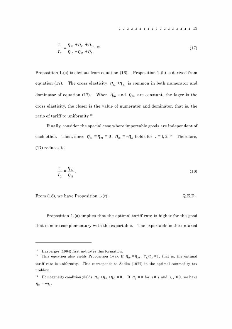
Proposition 1-(a) is obvious from equation (16). Proposition 1-(b) is derived from
equation (17). The cross elasticity 2112 ηη + is common in both numerator and
dominator of equation (17). When 10η and 20η are constant, the lager is the
cross elasticity, the closer is the value of numerator and dominator, that is, the
ratio of tariff to uniformity.13
Finally, consider the special case where importable goods are independent of
each other. Then, since 02112 ==ηη , iii ηη −=0 holds for 2,1 =i .14 Therefore,
(17) reduces to
11
22
2
1
ηη
ττ
= . (18)
From (18), we have Proposition 1-(c). Q.E.D.
Proposition 1-(a) implies that the optimal tariff rate is higher for the good
that is more complementary with the exportable. The exportable is the untaxed
12 Harberger (1964) first indicates this formation.13 This equation also yields Proposition 1-(a). If 2010 ηη = , 121 =ττ , that is, the optimal
tariff rate is uniformity. This corresponds to Sadka (1977) in the optimal commodity tax
problem.
14 Homogeneity condition yields 0210 =++ iii ηηη . If 0=ijη for ji ≠ and 0, ≠ji , we have
iii ηη −=0 .

14
good, and hence it is over-consumed. Taxation on the good that is more
complementary with the exportable partially offsets the over-consumption of the
exportable. Namely, Proposition 1-(a) shows that the ranking of tariff rates
depends upon the relative degree of complementarity between the taxed goods
(importable goods) and the untaxed good (exportable good). Since this was first
shown by Corllet and Hague (1953) in the context of commodity taxation, we will
call this the Corllet and Hague rule.
Proposition 1-(b) is called the Cross Substitutability Rule. The stronger is
cross substitutability between the taxed goods (i.e. the importable goods) creates
the stronger is the distortion.
Proposition 1-(c) is called the Inverse Elasticity Rule. This rule has been
them widely used in empirical estimates in the literature of optimal tariffs under
revenue constraints.
15
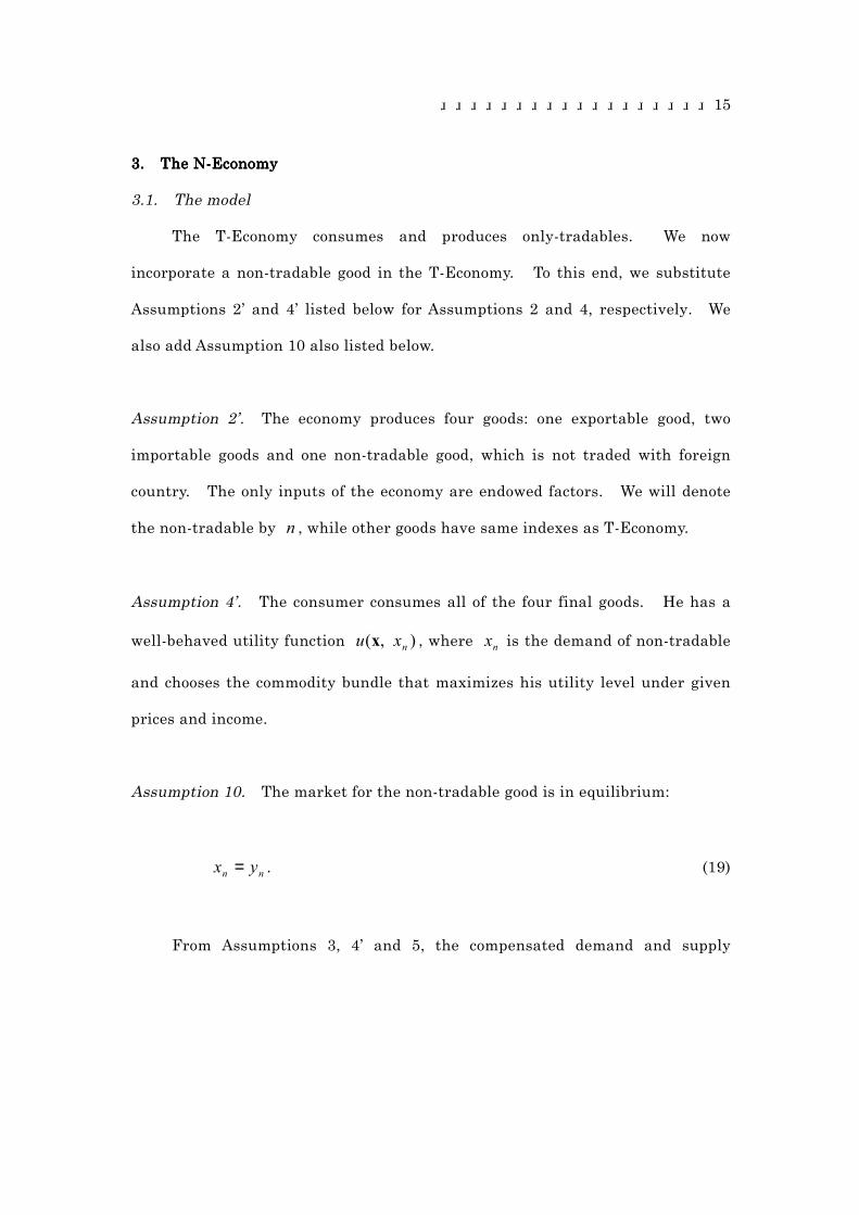
3.3.3.3. The N-EconomyThe N-EconomyThe N-EconomyThe N-Economy
3.1. The model
The T-Economy consumes and produces only-tradables. We now
incorporate a non-tradable good in the T-Economy. To this end, we substitute
Assumptions 2’ and 4’ listed below for Assumptions 2 and 4, respectively. We
also add Assumption 10 also listed below.
Assumption 2’. The economy produces four goods: one exportable good, two
importable goods and one non-tradable good, which is not traded with foreign
country. The only inputs of the economy are endowed factors. We will denote
the non-tradable by n , while other goods have same indexes as T-Economy.
Assumption 4’. The consumer consumes all of the four final goods. He has a
well-behaved utility function ),( nxu x , where nx is the demand of non-tradable
and chooses the commodity bundle that maximizes his utility level under given
prices and income.
Assumption 10. The market for the non-tradable good is in equilibrium:
nn yx = . (19)
From Assumptions 3, 4’ and 5, the compensated demand and supply

16
functions for the i -th good are given by15:
),,( uqxx nii q= ),2,1,0( ni = , (2’)
),( nii qyy q= ),2,1,0( ni = , (4’)
where nq is the price of the non-tradable. Since Assumptions 6 and 8 are
satisfied,
tpq += , and (5)
0)( =+−′ ryxp (7)
continues to hold. Assumptions 2’, 3, 4’ and 5 yield the budget constraint of the
private sector:
nnnn yqxq +′=+′ yqxq . (8’)
The N-Economy consists of (2’), (4’), (5), (7), (8’) and (19).
Equations (8’) and (19) yield the equation (8). Equation (8) in this economy
implies that the revenue from the sale of the tradable goods equal the consumer’s
spending on tradable goods. Thus the set of (8’) and (19) is equivalent to the set
15 Note that the utility function ),( nxu x is different from )(xu in T-Economy. However,
we will use the same notation to simplify the analysis. This is also applied to the
compensated demand, supply and excess demand function defined below. The vector of each
variable in this economy expresses the tradable good.

17
of (8) and (19). We will therefore represent this economy by equations (2’), (4’),
(5), (7) (8) and (19).
Definition 3. The economy satisfying Assumptions 1, 2’, 3, 4’, 5-9 and 10 is called
the N-Economy. When equation (2’), (4’), (5), (7), (8) and (19) are all satisfied, we
say that the N-Economy is in the full equilibrium.
The excess demand function in this economy is rewritten as
),(),,(),,( ninini qyuqxuqz qqq −≡ , ),2,1,0( ni = . (9’)
By substituting these functions for ii yx − and yx − in (7), (8) and (19), we have
0),,( =uqz nn q , (20)
0),,( =′ uqn qzq , (21)
0),,( =+′ ruqn qzp . (22)
Note that ),,( 210 zzz =′z is a vector of tradables, and do not contain nz . In
term of this notation, the N-Economy is in full equilibrium if and only if it
satisfies equations (5), (20), (21) and (22).
Equations (20), (21) and (22) contain four variables 1q , 2q , nq and u since
r is fixed by assumption. When one of the four variables are exogenously given,
the three equations determine the remaining variables. For example, if u is

18
given, the model determines the remaining variables ),,( 21 nqqq . Therefore,
from equation (5) we can find the tariff vector t that maximizes the utility level
u .
3.2. Optimal tariff in the N-Economy(I) : the general formula
We now define the following.
Definition 4. The tariff combination )( 21 tt , that maximizes the utility level u
in the model of (5), (20), (21) and (22) for a fixed level of r is called the optimum
tariff of the N-Economy.
The optimal tariffs in the N-Economy will be different from those in the T-
Economy because of the following differences between the models.
First, the N-Economy has two untaxed goods, i.e., the exportable and the
non-tradable, while the T-Economy has only one, i.e., the exportable good.
Second, a change in a tariff rate does not affect the price of the untaxed good
in the T-Economy, while it affects the price of an untaxed good, i.e., the non-
tradable, in tariffs in the N-Economy.
In view of the second difference, the optimal tax formula has to contain the
term representing the impact of a tariff change upon the price of the non-tradable.
To this end, we have to express nq as a function of 1q and 2q . Equation (20)
determines the price nq of the non-tradable good when q and u are exogenously
given. If equation (20) satisfies the conditions of the Implicit Function Theorem,
it can be solved for nq . The resulting function may be written as

19
),( uqq nn q= . (23)
Define the elasticity of the price of non-tradable with respect to the price of i -the
importable by
i
n
n
ini q
q
q
∂∂
=ˆ , (24)
and, the elasticity of the importable good i with respect to the price of non-
tradable by
i
innin z
zq=η .
Then the optimal tariff in the N-Economy can be stated in terms of this notation.
Theorem 2. In the N-Economy, the optimal tariff rate is expressed as
( )( )
( )( ) ,ˆ
,ˆ
11211221102
22121221201
∗
∗
−++++=
−++++=
θηηηηηητ
θηηηηηητ
nnnn
nnnn
q
q(25)
for some scalar 0>∗θ .
Proof. See Appendix 2 Q.E.D.

20
One difference between (13) and (25) is that (25) contains the terms niinjn q̂)( ηη −
representing the effect a change in a tariff rate upon the price of the untaxed good
through the change in the price of the non-tradable.
Taking the difference between the optimal tariff rates of the two goods in
(25), we have
{ }[ ] *212111022021 )ˆˆ)(()()( θηηηηηηττ nnnnnn qq +−++−+=− . (26)
3.3. Optimal tariff in the N-Economy (II) : independence between the
importables and the non-tradable
Let us first consider the special case where price changes of the importables
do not affect the prices of the non-tradables. Then
0ˆˆ 21 == nn qq , (27)
and hence
( )θηηηηττ )()( 11022021 nn +−+=− (28)
holds.
The expression n220 ηη + in the RHS of (28) represents the percentage
increase in the excess demand for the second importable when the prices of both of
the untariffed goods (i.e., 0 and n ) is simultaneous increased by one percent.
Thus it indicates the closeness of substitutability between the second importable

21
and the compound good consisting of the two untariffed goods. We can give a
similar interpretation to n110 ηη + . Equation (28) implies, therefore, that when
(27) holds in the N-Economy, the ranking of tariffs for the importables depends
upon their relative closeness of substitutability with the compound of the two
untariffed goods in this economy.16 This is a natural extension of Proposition 1-
(a), which shows that in the T-Economy, the ranking of tariffs for the importables
depends upon their relative closeness of substitutability with the untaxed good.
Equation (28) motivates the following definition.
Definition 5. The first importable good is the closer direct-substitute of the
untaxed goods than the second importable is, if
nn 220110 ηηηη +>+ ,
For equation (28) to hold, however, (27) is unnecessarily strong. It holds if
0ˆˆ 21 =+ nn qq (29)
16 Consider an economy where an additional exportable good is added to the T-Economy
without adding the non-tradable. If we denote the second exportable in this economy by n ,
then it can be readily shown that the counterpart of the optimal tariff formula of (13)
becomes
( )( ) ,
,
11221102
21221201
θηηηητ
θηηηητ
n
n
+++=
+++=
for some scalar 0>θ . The only change from (13) is that the terms n1η and n2η are added.

22
is satisfied. Totally differentiating (20) in nq and iq , while keeping other
variables constant, we obtain
nn
ni
i
n
z
z
q
q−=
∂∂
. (30)
Thus we have
02211 =+ nn zqzq (31)
if and only if (29) holds.
Definition 6. It is said that the composite of the importable goods is independent
of the non-tradable good if (31) holds.
It is needless to say that if (31) holds, a proportional increase in the prices of
the importable goods does not affect the net demand for the non-tradable good.
In terms of this definition, the following proposition holds:
Proposition 2. If the composite of the importable goods is independent of the
non-tradable, the following holds in the N-Economy:
(a) The optimal tariff rate is lower for the importable good that is the closer
From these, (28) holds also in this economy, as the counterpart of (15).

23
direct-substitute of the untaxed goods.
(b) The stronger is the cross-substitutability between importables, the closer is
the optimal tariff to uniformity when other elasticities are kept constant.
(c) The optimal tariff rate is inversely proportional to the own elasticity of
excess demand if the importables are independent of each other.
Proof. Proposition 2-(a) follows directly from (26) and (29). From (25) we have
( )( ) 1122112110
2212112220
2
1
ˆ
ˆ
nnnn
nnnn
q
q
ηηηηηηηηηηηη
ττ
−++++−++++
= , (32)
which proves (b). Next, consider the special case where importable goods are
independent of each other. Then, since 02112 ==ηη , 00 +++ iiini ηηη holds for
2,1 =i . Substituting this and (29) into (32), we have
( )( ) 22111
22122
2
1
ˆ
ˆ
nnn
nnn
q
q
ηηηηηη
ττ
−+−+
= ,
which proves (c). Q.E.D.
It is readily seen that if the independence between the composite of the
importable and the non-tradable is not assumed, Proposition 2-(a) and (c) no
longer hold.
3.4. Optimal tariff in the N-Economy (III) : the main proposition

24
Equation (26) may be rewritten as
( ) ( ) ( )( )[ ] *212112102021 ˆˆ θηηηηηηττ nnnnnn qq +−+−+−=− (33)
〔the original effect〕〔direct effect〕 〔indirect effect〕
Comparing (16) and (33), we find that the introduction of non-tradable brings
about two new terms: the direct effect, )( 12 nn ηη − and indirect effect,
)ˆˆ)(( 2121 nnnn qq +−ηη . These terms represent the difference in substitutability
between importable goods and non-tradable goods. The problem is that the sign
of the sum of the two new terms is not apparently clear, since the two terms can
have opposite signs. Indeed, we have
the direct effect )(0 12 nn ηη −< and
the indirect effect ))(ˆˆ(0 2121 nnnn qq ηη −+> ,
if niq̂ are positive and nn 12 ηη > . Does the indirect effect upset the direct effect?
The answer can be derived from the following.
Theorem 3. In the N-Economy, the optimal tariff rate is expressed as
,)ˆˆˆ(
,)ˆˆˆ(
1221012112102
1221022112201
∗
∗
+++++=
+++++=
θηηηηηητ
θηηηηηητ
nnnnnn
nnnnnn
qqq
qqq(34)

25
for some scalar 0>∗θ .
Proof. First apply Euler‘s Theorem to (20) to find
210 ˆˆˆ1 nnn qqq ++= .
From (this) we have
.ˆ)(
)ˆ1(ˆ
ˆˆˆ
2212
2221
122102
nnnn
nnnn
nnnnnn
q
qqq
ηηη
ηη
ηηη
−+=
−+=
++
Applying this to (25) yields the theorem. Q.E.D.
From the proof (34) it is clear that (25) and (34) are equivalent.
By taking the difference between 1τ and 2τ in (34), we have
[ ] ∗+−+=− θηηηηττ )ˆ()ˆ( 0110022021 nnnn qq (35)
A comparison between (35) and (33) shows that
)()ˆˆ)(()( 120212112 nnnnnnnnn qqq ηηηηηη −=+−+− .

26
From this, it follows that if 0ˆ 0 >nq , the sum of the direct and indirect effect has
the same as the direct effect, and hence the indirect effect does not quite upset the
sign of the direct effect.
Note that 0ˆ 0 >nq holds if the non-tradable is substitutable for the
exportable good, as is clear from (24) and (30).
Equation (35) motivates the following definition
Definition 7. The first importable good is the closer substitute of the untaxed
goods than the second importable is if
02200110 ˆˆ nnnn qq ηηηη +>+ . (36)
Hence optimal tariff rates can be ranked in terms of Definition 7.
We are in a position to state and prove the following Proposition.
Proposition 3. The following holds in the N-Economy:
(a) The optimal tariff rate is lower for the importable that is the closer
substitute of the untaxed goods.
(b) The stronger is the cross-substitutability between importables, the closer is
the optimal tariff to uniformity when other cross elasticities are kept constant.
(b’) The stronger is the cross-substitutability between the importable and the
non-tradable, the closer is the optimal tariff to uniformity, when other cross
elasticities are kept constant, provided that untaxed goods are independent of
each other

27
(c) The optimal tariff rate is inversely proportional to the own elasticity of
excess demand if and only if the importables are independent of each other, i.e.,
02112 ==ηη , and the importables are equally substitutable for the non-tradable,
i.e., nn 21 ηη = .
Proof. Equation (35) and Definition 7 immediately yield (a). From equation
(34), we also obtain
211201211210
211202211220
2
1
ˆˆ
ˆˆ
nnnnnn
nnnnnn
qqq
qqq
ηηηηηηηηηηηη
ττ
++++++++++
= .
Since the expressions in parentheses are common is both the numerator and the
denominator, the larger this term, the closer is the optimal tariff rates to
uniformity. This proves (b) and (b’).
If we assume that the importables are independent of each other, then
02112 ==ηη hold, and hence we have 00 =++ iniii ηηη . By substituting these
equations into (25), we have
11211
22122
2
1
ˆ)(
ˆ)(
nnn
nnn
q
q
ηηηηηη
ττ
−+−+
= . (37)
Equation (37) proves (c). Q.E.D.
Proposition 3-(a) is in line with the spirit of the Corlett and Hague Theorem. The
ranking of the optimal tariff rates of the two importable is again determined by

28
the ranking of substitutability between the two importables and the untaxed
goods(i.e., the exportable and the non-tradable). Proposition 3-(b) and (b’) show
that strong cross substitutability between the importables and between
theuntariffed goods tends to make the import tariffs to become closer to
uniformity. Proposition 3-(c) shows that if nn 12 ηη ≠ , the Inverse Elasticity Rule
does not hold.17
17 See Hatta (1986) and (1994).

29
5. Concluding remark5. Concluding remark5. Concluding remark5. Concluding remark
The optimal tariff problem in small open economy has been studied for
models with one untaxed good. The present paper introduced the second
untaxed good whose domestic price changes endogenously. It was observed that
the celebrated Inverse Elasticity Rule is no longer valid in this situation. Often
this rule is used as practical guide to obtain a rough estimate of the optimal tariff
rates. In the economy with endogeneous price change, however, the rule fails to
give such a guide.
On the other hand, it was observed that the Cross Substitutability Rule and
the Corlett and Hague Rule are quite robust in the new situation. These rules
seem to give qualitative and quantitative insights into the optimal tariff rates in
practical situation.

30
AcknowledgmentsAcknowledgmentsAcknowledgmentsAcknowledgments
We would like to thank Professors Kenzo Abe, Takashi Fukushima,
Yoshiyasu Ono, Koji Shimomura, Katsuhiko Suzuki and Makoto Tawada for their
invaluable comments on several earlier drafts of this paper.

31
Appendix 1Appendix 1Appendix 1Appendix 1: uniform and p: uniform and p: uniform and p: uniform and proportionalroportionalroportionalroportional tariffs tariffs tariffs tariffs
In this appendix, we will prove that no tariff structure for a given
government revenue can achieve an efficient resource allocation.
A tariff stricture is called uniform, if all importable goods share an identical
ad valorem tariff rate, i.e., if 00 =t , and if
β=i
i
q
t, )2,1( =i , (A1-1)
holds for some scalar β .
Under uniform tariff structure, domestic prices of the exportable goods are
equal to world prices, while those of the importable goods are proportionally
higher than the world prices. Thus a uniform tariff structure generates
distortions, and the resource allocation is not efficient. However, a uniform tariff
can raise a given tariff revenue. Its resource allocation is, however, not efficient,
because it is not proportional.
On the other hand, a tariff structure is called proportional if all tradable
goods i.e., including exportables share an identical ad valorem tariff rate, i.e., if
β=i
i
q
t, )2,1,0( =i , (A1-2)
holds for some scalar β . Under a proportional tariff structure, domestic prices
of both exportables and importables are proportional to their world prices.

32
Subsidies are given to the export of the exportable goods at the same rate as
import tariffs. Thus the domestic prices of the exportables are higher than the
world prices. The proportional tariff attains an efficient resource allocation.
A proportional tariff structure, however, yields zero revenue. Under the
proportional tariff, from (A1-2) and (5), we have
pq ψ= (A1-3)
where βψ += 11 . Substituting (A1-3) into (7) yields
0=′zp . (A1-4)
From (A1-4), we obtain 0=r .
This implies that the revenue collected by import tariffs is all spent on export
subsidies. Namely, collecting a given tariff revenue necessarily generates a
distortion. It is the revenue-constrained optimal tariff structure that minimizes
this distortion.
33
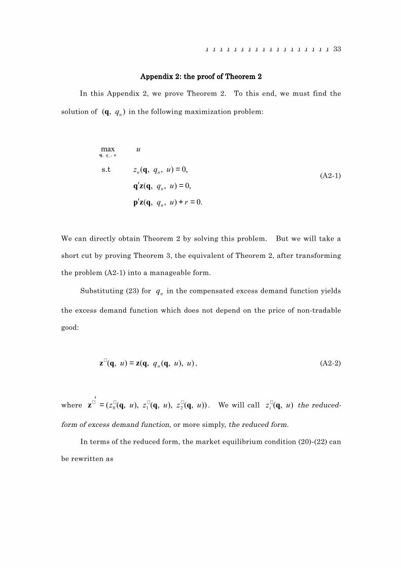
Appendix 2Appendix 2Appendix 2Appendix 2: the proof of Theorem 2: the proof of Theorem 2: the proof of Theorem 2: the proof of Theorem 2
In this Appendix 2, we prove Theorem 2. To this end, we must find the
solution of ),( nq q in the following maximization problem:
.0),,(
,0),,(
,0),,(
max,
=+′
=′
=
ruq
uq
uqz
u
n
n
nn
uqn
s.t
,
qzp
qzq
q
q
(A2-1)
We can directly obtain Theorem 2 by solving this problem. But we will take a
short cut by proving Theorem 3, the equivalent of Theorem 2, after transforming
the problem (A2-1) into a manageable form.
Substituting (23) for nq in the compensated excess demand function yields
the excess demand function which does not depend on the price of non-tradable
good:
)),,(,(),( uuqu n qqzqz =∗ , (A2-2)
where )),(),,(),,(( 210 uzuzuz qqqz ∗∗∗∗ =′. We will call ),( uzi q∗ the reduced-
form of excess demand function, or more simply, the reduced form.
In terms of the reduced form, the market equilibrium condition (20)-(22) can
be rewritten as

34
0),( =′ ∗ u qzq , (A2-3)
0),( =+′ ∗ ru qzp . (A2-4)
These two equations contain three variables, 1q , 2q and u . The market
equilibrium conditions (A2-3) and (A2-4) in terms of the reduced form are
equivalent to those in terms of (20), (21) and (22).
Thus (A2-1) is transformed into
.0),(
,0),(
max,
=+′
=′
∗
∗
ru
uu
u s.t
qzp
qzq
q
(A2-5)
This is formally identical to (14), and hence we immediately obtain the following
optimal tariff rates exactly in the same manner as in Theorem 1.
Lemma 1. In the N-Economy, the optimal tariff rate is expressed as
,)(
,)(
2112102
2112201
∗∗∗∗
∗∗∗∗
++=
++=
θηηητ
θηηητ(A2-6)
where ))(( 21222112121∗∗∗∗∗∗∗ −−= zzzqqzzαθ and ∗
ijη is the elasticity of the i -th
reduced with respect to the price jq .

35
Let us now decompose ∗ijη into terms involving ijη and inη . By partially
differentiating (A2-2) with respect to jq , we have
j
n
n
i
j
i
j
i
q
q
q
z
q
z
q
z
∂∂
⋅∂∂
+∂∂
=∂∂ ∗
. (A2-7)
The first term in the RHS represents the effect of the price change of j -th good
upon the excess demand of i -th good. We will call this the direct effect. The
second term represents the effect of the price change of j -th good upon i -th good
through the price change of the non-tradable. We will call this the indirect effect.
Thus, the LHS of (A2-7) represents total effect including direct and indirect effect.
By rewriting (A2-7), we obtain
njinijij q̂ηηη +=∗ . (A2-8)
The term ijη and njin q̂η correspond to the direct and indirect effect, respectively.
Substituting equation (A2-8) into (A2-6), we have equation (34), and hence
(25). This result and the following Lemma prove Theorem 2.
Lemma 2. 0>∗θ . 18
18 We are grateful to Professor Suzuki of Kwansei Gakuin University for suggesting this
proof.

36
Proof. The term ∗θ has the same sign as government revenue r , if
=
∗∗
∗∗
2221
1211*
zz
zzZ is negative semi-definite. See Daimond and Mirrlees (1971,
p.262). From equation (A2-7),
−−
−−=∗
nn
nn
nn
nn
nn
nn
nn
nn
z
zzz
z
zzz
z
zzz
z
zzz
Z22
2212
21
2112
1111
.
From the property of matrix, we find
nnn
n
nnnn
nn
zzzz
zz
zzzZ
1
11111111
1=−=∗ , and
nnnn
n
n
nn
nn
nn
nn
nn
nn
nn
nn
nn
zzzzzzzzz
zz
zzz
z
zzz
z
zzz
z
zzz
Z
21
22221
11211
2222
1221
2112
1111
2
1=−−
−−=∗ .
If ),,( uqz ni q is concave with respect to ),( nq q , 01 <∗Z and 02 >∗Z . Thus,
since ∗Z is the negative semi-definite, ∗θ is positive. Q.E.D.
Incidentally, inequality (36) can be equivalently written as
∗∗ > 2010 ηη .

37
From (A2-8), In Definition 7, therefore, (36) can be replaced by the above
inequality.

38
ReferencesReferencesReferencesReferences
Auerbach, A. J. (1985) “The Theory of Excess burden and Optimal Taxation,” in A.
J. Auerbach and M. Feldstein, eds., Handbook of Public Economics,
Amsterdam: North-Holland.
Corlett, W. C. and D. C. Hague (1953) “Complementarity and the Excess Burden
Taxation,” Review of Economic Studies, Vol. 21, pp. 21-30.
Dahl, H. S. Devarajan and S. van Wijnbergen (1986) “Revenue-Neutral Tariff
Reform: Theory and an Application to Cameroon,” Country Policy
Department Discussion Paper, No. 1986-25, World Bank,May, processed
, and (1994) “Revenue-Neutral Tariff Reform:
Theory and an Application to Cameroon,” Economic Studies Quarterly,
Vol.45, No. 3, pp. 213-226
Dasgupta, P. and J. Stiglitz (1974) “Benefit-Cost Analysis and Trade Policies,”
Journal of Political Economy, Vol. 82, pp. 1-33.
Diamond, P. A. and P. A. Mirrlees (1971) “Optimal Taxation and Public Production
I and II,” American Economic Review, Vol. 61, pp. 8-27 and pp.261-278.
Graaff, J. (1949-50) “On Optimum Tariff Structures.” Review of Economic Studies
17, no.42, pp.47-59.
Lopez, R. and A. Pnagariya (1992) “On The Theory of Piecemeal Tariff Reform:
The Case of Pure Imported intermediate Input,” American Economic
Review, Vol. 82, pp. 615-625.
Harberger, A. C.(1964) “Taxation, Resource Allocation and Welfare,” in The Role
Direct and Indirect Taxes in the Federal Reserve System, Princeton
University Press for the National Bureau of Economic Research and the
Brookings Institution.
39
Hatta, T. (1986) “Welfare Effect of Changing Commodity Tax Rates toward
Uniformity,” Journal of Public Economics, Vol. 29, pp. 99-112.
(1993) “Four Basic Rules of Optimal Commodity Taxation,” in Ali M
El-Agraaed,ed, Public and International Economics, St. Martins Press, pp.
125-147.
(1994) “Why Not Set Tariffs Uniformly Rather Than Optimally,”
Economic Studies Quarterly, Vol. 45, No. 3, pp. 196-212.
Heady, C. J. and P. K. Mitra (1987) “Distributional and Resource Raising
Arguments for Tariffs,” Journal of Development Economics, Vol. 20, pp.
77-101.
Johnson, H.G. (1953-54) “Optimum Tariffs and Retaliation.” Review of Economic
Studies 21, no.55, pp.152-153.
Mitra, P. K. (1994) “Protective and Revenue Raising Trade Taxes: Theory and an
Application to India,” Economic Studies Quarterly, Vol. 45, No. 3, pp.
265-287.
Pnagariya, A. (1992) “Input Tariffs, Duty Drawbacks and Tariff Reform,” Journal
of International Economics, Vol. 32, pp. 132-147.
(1994) “Why and Why-Not of Uniform Tariffs,” Economic Studies
Quarterly, Vol. 45, No. 3, pp. 227-245.
Rajaram, A. (1994) “Tariff and Tax Reforms-Do World Bank Recommendations
Integrate Revenue and Protection Objectives?” Economic Studies
Quarterly, Vol. 45, No. 4, pp. 321-338.
Ramsey, E. (1927) “A Contribution to the Theory of Taxation,” Economic Journal,
Vol. 37, pp.47-61.
Sadka, E. (1977) “A Theorem on Uniform Taxation,” Journal of Public Economics,

40
Vol. 7, pp. 387-391.
Recommended