DG-IV Document - October 2015 1 | P a g e
Fig. 1: DG‐IV Categories (illustrative)
OVERVIEW & SUMMARY In recent years, distributed generation (DG) resources have rapidly grown in number and are playing an increasingly important role alongside traditional generation resources. From a national perspective, renewable energy growth is trending upward, although cost competitiveness and customer adoption rates of renewable resources vary by geographic region. TVA has recognized this transitional market shift towards greater renewable energy and DG adoption and has developed a methodology to determine a Distributed Generation ‐ Integrated Value, or DG‐IV. Desired Outcome TVA’s desired outcome is to develop a comprehensive methodology that assesses both the representative benefits and costs associated with various forms of DG. The methodology components are intended to be grounded in solid, quantifiable, and defensible analytics, and serve as a robust basis for DG valuation. Although the numerical values associated with each methodology component will need to be updated to adjust to changing market conditions, the components themselves should remain relevant over time.
As is demonstrated in Table 5 on page 23, the methodology adopted in this report includes cost and benefit components that accrue to the utility. The combination of these components, represented in green in Table 5, equate to the solar‐specific avoided cost to TVA. As described below, additional benefits or costs may be applied as part of the later program design phase or as future placeholder topics. The primary focus of this effort was to select the DG‐IV methodology components, but also develop a firm analytical basis for calculating each component (green components). Within each of these categories the individual components may deliver a net benefit or cost. This versatile approach establishes a robust foundation that can be built upon to adapt to changing conditions. In the end, the DG‐IV methodology establishes a representative set of building blocks used to evaluate and quantify various DG resources.
Initial Focus: Small‐Scale Solar Due to the increasing popularity and growing awareness of solar photovoltaic (PV) energy, solar PV was selected as the most representative DG resource type to evaluate. Concepts utilized in existing “Value of Solar” processes were leveraged to identify value stream components that are directly applicable and representative of the Tennessee Valley region. A maximum solar PV system size of 50 kW was selected for use with this DG‐IV methodology to align with TVA’s current solar PV deployment activities at the residential and small commercial scales.

DG-IV Document - October 2015 2 | P a g e
Transparency
• Accessibility to the information
• Data, assumptions, calculations • Clear and well‐defined
• Information provided in a timely manner with sufficient time for engagement
Fairness
• Views all stakeholders on an equal footing
• Compromise in process
• Inventory and consider all variables
Adaptability
• Broadly applicable to multiple forms of distributed resources
• Continuous learning process
• Evolving in a positive way over time
Versatility
• Continues to work in a changing technology and business environment
• Ensures implementation to a widespread, robust set of markets
• Provides potential for differentiation so it works for a wide array of customers, locations, and environments
We will develop a quality, actionable process that accomplishes:
Fig. 2: DG‐IV Process Principles
DG‐IV Group Participation & Meetings To develop the DG‐IV methodology, TVA assembled a diverse cross‐section of regional participants from the Tennessee Valley region. Local power companies (LPCs) served by TVA, the Tennessee Valley Public Power Association (TVPPA), various environmentally‐focused non‐governmental entities, solar industry representatives, academia, state governments, and national research institutions were represented. To provide objective and independent third‐party facilitation and subject matter expertise, TVA contracted the Solar Electric Power Association (SEPA). Additionally, the Electric Power Research Institute (EPRI) took the lead role in analyzing distribution system impacts and losses. This analysis directly aligns with EPRI’s innovative ‘Integrated Grid’ Initiative (www.epri.com/integratedgrid). EPRI’s technical rigor not only provides insight into the DG‐IV process, but helps provide understanding within the broader context of DG integration. Involvement of external participants in the DG‐IV process officially began on April 23, 2014. As part of the initial meeting, guiding principles were developed based on group collaboration and agreement on the overall intent and process (shown in Figure 2). These principles encompass the four core values of transparency, fairness, adaptability, and versatility. These principles are shown at the beginning of every meeting to ensure conversation is grounded upon a unified platform of collaborative consensus building. Subsequent meetings are detailed in Table 1 (located on following page).

DG-IV Document - October 2015 3 | P a g e
Table 1: DG‐IV Group Meetings
Item Date Meeting Objectives & Goals Meeting # 1 April 23, 2014 DG‐IV group kick‐off meeting
Webinar # 1 May 15, 2014 EPRI Distribution impact overview and discussion
Meeting # 2 June 5‐6, 2014 Initial deep dive: DG‐IV components and calculations
Meeting # 3 July 9, 2014 Follow‐up: DG‐IV components and calculations
Meeting # 4 Aug 27‐28, 2014 Initial calculation methodology, inputs, and draft results
Webinar # 2 Oct 31, 2014 Draft report review summary and EPRI distribution update
Meeting # 5 Dec 3, 2014 Finalize DG‐IV Methodology
Meeting #6 July 2, 2015 Share Final Draft DG‐IV Report
Future Application & Considerations The DG‐IV methodology will serve as an effective input, along with other factors, to inform future TVA renewable energy decisions. Additionally, TVA’s 2015 IRP study is expected to provide valuable insight regarding the future direction and associated volumes of various generation resource options. More specifically, the IRP will help inform TVA how solar PV resources compete with other generation sources across multiple future strategies and scenarios. Although the DG‐IV methodology and the 2015 IRP will help provide important overall guidance, these inputs will not dictate specific renewable implementation details, such as annual capacity targets or renewable pricing structures. Ultimately, final program offering decisions consider various interrelated factors beyond the considerations of both the DG‐IV and IRP processes. Other practical considerations should also be weighed when attempting to broadly apply the results of this study in assigning a “value” to DG resources. These considerations include the uncertain nature of legislative and regulatory environments, the lack of a regulatory basis or industry consensus on selecting appropriate DG valuation components, and the many unknowns or unintended consequences that can arise when DG assets are added to a distribution system that did not originally envision two‐way power flow. The issuance of this report is an important first step towards realizing a DG‐IV methodology for the Tennessee Valley region, but caution should be taken in its application until more data is acquired and analyzed and greater regulatory and cost certainty becomes available. During the development of the methodology for assigning a value to distributed resources, TVA and individuals on the stakeholder group identified a number of policy issues that are outside of the context of this work. While the components of the value have been explored and initial results determined, we have not attempted to account for system or marketing decisions that TVA and the LPC’s would engage in that could increase the price offered for solar. For example, we might put an incentive on the value for location or for providing ancillary services; or TVA might decide that stimulating the market is the right thing to do and add an incentive to make it easier for the market to transact. Reducing the uncertainty around the price signal for distributed solar depends on the policies that TVA decides it should include as part of the pricing scheme, but this policy framework builds on the value methodology rather than changes it. Some of the policy issues that will be considered as part of the implementation include how to set a framework for identifying and assessing broader environmental
DG-IV Document - October 2015 4 | P a g e
impact/benefit, recognizing the ancillary services value, identifying economic development benefits, and quantifying system security enhancements and disaster recovery capabilities.
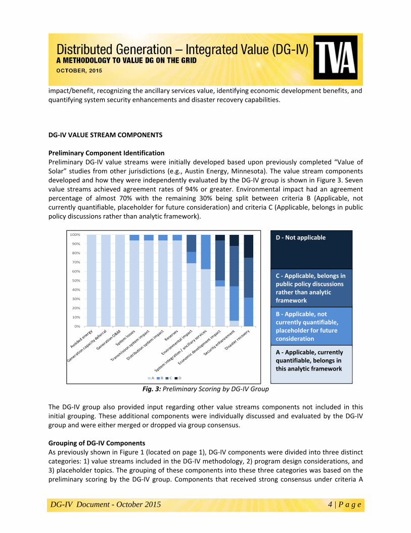
DG‐IV VALUE STREAM COMPONENTS Preliminary Component Identification Preliminary DG‐IV value streams were initially developed based upon previously completed “Value of Solar” studies from other jurisdictions (e.g., Austin Energy, Minnesota). The value stream components developed and how they were independently evaluated by the DG‐IV group is shown in Figure 3. Seven value streams achieved agreement rates of 94% or greater. Environmental impact had an agreement percentage of almost 70% with the remaining 30% being split between criteria B (Applicable, not currently quantifiable, placeholder for future consideration) and criteria C (Applicable, belongs in public policy discussions rather than analytic framework).
Fig. 3: Preliminary Scoring by DG‐IV Group
The DG‐IV group also provided input regarding other value streams components not included in this initial grouping. These additional components were individually discussed and evaluated by the DG‐IV group and were either merged or dropped via group consensus. Grouping of DG‐IV Components As previously shown in Figure 1 (located on page 1), DG‐IV components were divided into three distinct categories: 1) value streams included in the DG‐IV methodology, 2) program design considerations, and 3) placeholder topics. The grouping of these components into these three categories was based on the preliminary scoring by the DG‐IV group. Components that received strong consensus under criteria A
0%
10%
20%
30%
40%
50%
60%
70%
80%
90%
100%
A B C D
B ‐ Applicable, not currently quantifiable, placeholder for future consideration
C ‐ Applicable, belongs in public policy discussions rather than analytic framework
D ‐ Not applicable
A ‐ Applicable, currently quantifiable, belongs in this analytic framework

DG-IV Document - October 2015 5 | P a g e
(Applicable, currently quantifiable, belongs in this analytic framework) were put into the first category (DG‐IV methodology). Other components were divided into the other two categories. Table 3 identifies the specific components that are included within each of these categories and provides a brief description of each component. The primary purpose of the DG‐IV process is to solidify the first category (methodology), since the core focus of this work is to develop a versatile and repeatable DG valuation method. The other categories are relevant as they provide a basis for potential consideration either within program design or as future DG‐IV methodology components.

DG-IV Document - October 2015 6 | P a g e
Table 3: Categorization of DG‐IV Components
Categories Components Description
Included in DG‐IV
Methodology
Generation Deferral (Capital & Fixed Operations & Maintenance)
The marginal system capacity and fixed operations and maintenance value of deferred generation additions (including reserves) due to DG
Avoided Energy (Fuel, Variable Operations &
Maintenance, Start‐up)
The marginal system energy, fuel, variable operations and maintenance, and start‐up value of generation displaced by DG
Environmental (Compliance & Market)
Compliance ‐ addresses regulatory compliance components that are incorporated as part of TVA’s system portfolio analysis (e.g., CO2, coal ash, cooling water) Market ‐ the individual market value a DG resource adds to the valuation methodology in addition to regulatory compliance value (e.g., renewable energy credits)
Transmission System Impact
Net change in transmission system infrastructure due to presence of DG (i.e., transmission required, deferred, or eliminated)
Distribution System Impact
Net change in distribution system infrastructure due to presence of DG (i.e., distribution required, deferred, or eliminated)
Losses (Trans. & Distr.)
Net change in transmission and distribution system losses due to presence of DG
Program Design
Considerations
Local Power Company(LPC) Costs & Benefits
Associated costs of implementing renewable energy programs (e.g., administrative, operational, engineering), and potential LPC‐specific distribution system benefits
Economic Development Regional job and economic growth caused by DG growth
Customer Satisfaction Enhanced customer value due to preference, optionality, or flexibility
Local Differentiation Site‐specific benefits and optimization (e.g., geographic location, placement & optimization of distribution grid, load demand reduction)
Placeholder Topics
System Integration/ Ancillary Services
The symbiotic value of smart grid resources and high levels of DG penetration, and cost of integration of non‐dispatchable resources ‐ further study and data required
Additional Environmental Considerations
Additional environmental factors that are not specifically addressed as part of the environmental compliance or market values
Security Enhancement Increased system resiliency to reduce power outages and rolling blackouts due to presence of DG
Disaster Recovery The ability and pace of DG assets to assist with system restoration after significant damages caused by natural disasters
Technology Innovation Impact value associated with technology‐driven investment in DG

DG-IV Document - October 2015 7 | P a g e
DG‐IV CALCULATIONS Comparing Solar PV to Traditional Generation Resources It is important to consider applicable differences between solar PV and traditional energy resources. These differences include both benefits and challenges that not only require identification, but also analytical interpretation into quantifiable values. Some of the primary benefits associated with solar energy compared to conventional power plants include: scalability and locational versatility, elimination of fuel costs, and emissions‐free generation. Scalability and locational versatility are addressed at some level with regards to transmission and distribution impacts and losses. Capacity sizing and locational‐specific siting of solar PV facilities to more effectively accommodate the needs of the distribution system may also be addressed via renewable program design or other utility implementation strategies. Elimination of fuel costs is addressed via avoided energy calculations, which includes consideration of fuel price hedging capability and the associated avoidance of volatility risk of natural gas prices. Lastly, emissions‐free generation provides various environmental benefits, but has its own environmental impacts. These benefits are realized over the life of the solar PV system, which typically exceeds 25 years.1 The merit of considering a 25 year life was discussed by the group, however this would exceed TVA’s typical contractual terms for generation. TVA’s contract terms for power purchase agreements are typically for 20 years or less because this provides a reasonable balance between TVA’s power supply planning and financial planning risk tolerance and 3rd party market attractiveness. Some of the primary challenges associated with solar energy include: intermittent generation, inability to dispatch, and an inability to control when generation is produced (a.k.a. “must take” energy). Intermittent generation, or energy that is not continuously available, is primarily an operational concern that depends on real‐time generation profiles. To address these concerns from a system‐wide portfolio perspective, solar energy profiles are compared against historic TVA load profiles to determine how much of the capacity can be deemed as being “net‐dependable capacity”, or NDC. The NDC value indicates how much capacity is counted towards offsetting TVA’s peak demand requirements, which currently occur in the summer months. As part of the 2015 Integrated Resource Plan (IRP) process, the summer NDC value was determined to be 50% for fixed‐axis solar PV (see the Technical Appendix for more details). The NDC value is relevant to the portfolio analysis process, since TVA is currently a summer peaking utility. If TVA’s system transitioned to primarily winter peaking, the value would likely be at or near zero since our system peak in the winter is during the 7:00 am hour Eastern Time. The inability to dispatch solar energy also changes operational expectations, specifically with regard to how and where other generation resources are dispatched. This concern is somewhat addressed via the NDC correction, but future work is needed to best understand possible operational impacts.
1 Solar panels typically have a 25-year warranty. National Renewable Energy Laboratory. Solar Ready Buildings Planning Guide. December 2009. Found at: http://www.nrel.gov/docs/fy10osti/46078.pdf

DG-IV Document - October 2015 8 | P a g e
Solar PV along with other “must take” energy sources, such as wind, provides less system operations flexibility when compared to traditional dispatchable resources. Solar PV generation is a function of solar irradiance which is considered a variable fuel source. Therefore, to meet the needs of continuous energy loads on the utility grid, traditional sources such as natural gas must be dispatched to fill in any “gaps” in solar energy generation profiles. During clear sky conditions, solar generation profiles are fairly manageable, however during irregular cloud pattern conditions, dynamic solar capacity ramping events can occur repeatedly. This generation volatility and reliability risk is greater for large utility‐scale solar PV projects but still exists for distributed solar generation. However, this risk is somewhat mitigated under the scope of this methodology, which targets small‐scale solar deployment that is more evenly distributed across the distribution network. Traditional resources are still needed to back‐up variable generation conditions associated with solar PV generation when the sun is not shining or during nighttime hours. The cost of this “backup generation” is included in the methodology and is addressed through a combined analysis of generation deferral and avoided energy that recognizes both the solar energy profile and the contribution of solar resources at the time of the system peak. While some think this backup generation should cost more than we have computed in this methodology, others believe it is not necessary. DG‐IV Calculation Method After selecting the components to be included in the DG‐IV methodology, calculation approaches and associated boundary conditions were identified to derive individual component values. Generation Deferral (Capital & Fixed O&M) Capital deferral relates to the deferral of new generation capacity, typically from a natural gas combustion turbine or combined cycle asset. This deferral results in both capital and fixed operations and maintenance (O&M) savings. Capital and fixed O&M costs can vary substantially based on the type of asset deferred and the timing of the deferral. As part of TVA’s resource planning process, capacity expansion and production cost models are utilized as strategic tools in making future generation assets decisions. The overarching goal of both of these models is to minimize the net present value of TVA’s total system cost. A visual reference of how these models interact is shown in Figure 4.
Fig. 4: Resource Planning Modeling Process

DG-IV Document - October 2015 9 | P a g e
Fig. 5: Generation Deferral (annual average)
Fig. 6: Avoided Energy (annual average)
Total plan costs are first examined according to TVA’s existing base case scenario. Then, 2,000 MW 2 of solar PV (AC‐rated) was added to TVA’s generation resources in the first year of the evaluation period (2015) at no cost. This capacity value was selected to represent a significant amount of solar PV adoption that would have a material impact on the modeling results (the capacity expansion plan). The differential in cost between the base case and solar PV scenario provides an indication of the value of solar PV on the TVA system. This system‐wide analysis method, which is applied over a 20‐year term (2015‐2034), is an effective means of determining a value that is specific to TVA’s capacity and generation additions forecast. The system analysis approach is not only effective in determining generation deferral, but also avoided energy and a system environmental value. Regarding solar PV capacity, 1,000 MW (net dependable capacity value) are applied toward meeting TVA’s resource adequacy requirements, including its 15% reserve margin target. The ten‐year average capital and fixed O&M costs that would be avoided by 1,000 MW AC of solar are shown in Figure 5. The increases over the second ten year period are a result of customer energy growth which create the need for additional summer capacity. Solar additions help offset expected spending on assets that provide system capacity. In this particular analysis reference case, the calculated levelized value for the generation deferral value is 1.53 cents/kWh. Avoided Energy (Fuel, Variable O&M, Start‐up) Avoided energy values are derived from the system‐wide analysis approach mentioned previously. Similar to capacity deferral, when new generation is deferred there are associated savings from the following components: fuel, variable operations and maintenance, and start‐up costs for the total generation fleet. The model is currently limited to an hourly time step so there may be intra‐hour impacts not captured at in this analysis. Unlike firm
2 Number used for modeling purposes; not indicative of program targets.

DG-IV Document - October 2015 10 | P a g e
Fig. 7: Environmental Sections
(illustrative)
capacity requirements associated with capacity deferral (discussed above), 100% of the solar PV energy profile is applied towards the avoided energy value. As seen in Figure 6, fuel costs account for most of the total avoided energy value. As commodity fuel costs increase over time, the avoided energy value related to fuel also increases. Fuel, variable O&M (VOM), and start‐up costs3 can vary substantially based on the type of asset deferred and the timing of the deferral. For example, because more coal generation is avoided in the first ten years, VOM savings are higher than the second ten year period when more natural gas generation is avoided. For this particular analysis reference case, the calculated levelized value for the avoided energy value is 4.58 cents/kWh. As part of this analysis, fuel volatility and associated fuel price risk were also explored. TVA’s internal analysis, which simulates generation costs via different scenarios, found that solar PV additions can yield slightly greater avoided costs during high summer load conditions with high marginal fuel prices. Conversely, solar PV additions can also result in slightly less avoided costs in situations with low loads and low marginal fuel prices. TVA determined that these upside and downside conditions tend to offset each other as part of a balanced base case planning scenario and generally apply to any fixed‐price generation or hedge. A DG‐IV participant conducted a separate analysis by examining the change in fuel savings from solar (which has zero fuel cost) under periods of natural gas price run‐ups and decreases compared to the base price forecast. The effect using New York Mercantile Exchange (NYMEX) contract options as well as simulations of generation cost found that when using a two‐tailed probability distribution, the volatility value was either entirely dependent on forecasts of NYMEX market options or cancelled out over time. As a result, no material fuel volatility value was included in the methodology at this time. Environmental Of all the categories discussed, the environmental category garnered the most discussion. After much deliberation and discussion by the DG‐IV group, the group decided to divide the environmental component into three distinct sections (Figure 7):
1) Environmental Compliance Value ‐ addresses regulatory compliance components that are incorporated as part of TVA’s system portfolio analysis 2) Environmental Market Value ‐ the individual market value a DG resource adds to the valuation methodology in addition to regulatory compliance value (e.g., renewable energy credits) 3) Additional Environmental Considerations – Additional environmental factors that are not specifically addressed as part of the environmental compliance or market values
3 Start-up costs capture the number of times units are cycled

DG-IV Document - October 2015 11 | P a g e
The DG‐IV group reached unanimous consensus on the inclusion of the first two topics within the DG‐IV methodology (shown in green). Consensus was not reached by the group on the third topic (shown in orange). However, group participants did decide that it was important to document the various opinions associated with the third topic. As potential regulations and future markets evolve, individual items captured within the ‘additional environmental considerations’ topic could become avoided costs to the utility, and thus transition into either the environmental compliance or market value as deemed appropriate. Environmental Compliance Value The environmental compliance value is consistent with the system‐wide analysis method utilized in calculating generation deferral and avoided energy. TVA’s production cost model is leveraged to calculate the impacts of known environmental regulations whose compliance costs can be discretely itemized. Some compliance‐related costs are already inherently captured in the model based on both historical and forward‐looking asset decisions. These compliance values address topics such as coal ash management, cooling water, mercury, air pollution, and water discharges and are embedded calculations which are difficult to disaggregate and independently value. Environmental regulatory programs limit or restrict outputs from fossil generation that depend in large part on the actual use of fossil assets. Carbon dioxide emissions provide a good surrogate for fossil system generation. For these reasons, the environmental compliance value is based upon the carbon intensity of the generation assets deferred. TVA assumes a CO2 compliance cost curve in terms of dollars per ton of CO2 equivalent beginning in 20224. The actual value is based on the carbon intensity of the avoided fuel combustion, which depends on the type of fuel and efficiency of the generating unit.
For example, coal deferrals result in a greater environmental compliance value than gas deferrals due to higher carbon content of coal than natural gas per electricity generated. As future environmental legislation or regulations develop, the environmental compliance value will also adjust to reflect these changes. The calculated levelized value for the environmental compliance value is 0.22 cents/kWh. Environmental Market Value The environmental market value refers to the individual value a DG resource adds to the valuation methodology, which is not expressly captured as part of the system portfolio analysis. Renewable energy is unique due to the fact that a market mechanism exists to help stimulate its ongoing development. To address this additional market value, renewable energy credits (REC) and carbon markets were considered to identify an appropriate market opportunity value. A REC is defined as a tradable, non‐tangible energy commodity that represent evidence that 1 megawatt‐hour (MWh) of electricity was generated from an eligible renewable energy resource. Carbon accounting associated with the indirect CO2 emissions is inextricably linked within the solar REC (SREC) and cannot be separated. Unlike solar PV, landfill gas assets have an additional carbon offset value, in addition to the REC itself, and these commodities can be treated separately and therefore
4 Based on assumption developed collaboratively in TVA’s IRP process and used here for consistency

DG-IV Document - October 2015 12 | P a g e
monetized independently. To determine an environmental market value for solar PV, only one voluntary market can be utilized to assign a market opportunity value. Voluntary carbon markets currently exist but have limited market maturity. REC markets are more established and vary based upon the applicable market (compliance or voluntary) and resource type (e.g., solar REC or wind REC). Since a large majority of TVA’s service territory is free of Renewable Portfolio Standards (RPS) compliance obligations (North Carolina being the exception), the voluntary REC market was selected as a representative proxy. SREC prices can vary dramatically within various compliance markets and in comparison to other renewable resource types. In voluntary markets, REC prices vary, but with much less price differentiation between resource types. Based on current and near‐term REC quotes5, national voluntary SREC markets are trading between $3‐$5/MWh per REC, while National voluntary RECs (any resource type) are closer to $1/MWh. The primary differences between these two markets are trading volume and liquidity. Currently, national voluntary SREC markets are trading at fairly low volume levels. According to REC market analysts6, trading of only 140 MW AC solar PV (~7% of the value explored in this methodology) could create imbalances to the national voluntary SREC market. Additionally, trading would need to occur as several discrete transactions between 1 to 10 MW AC in scale. In contrast, the National voluntary “any REC” markets can handle well in excess of the solar PV capacity explored in this methodology. For these reasons, TVA has applied a $1/MWh REC value for this component with a 1.9% escalation that is consistent with TVA’s IRP process. This value is carried from the first year in this analysis through the year before carbon compliance is applied (2015‐2021). After 2021 it is assumed that the REC would need to be retired to meet compliance obligations. The calculated levelized value for the environmental market value is 0.11 cents/kWh. This valuation is based upon current, voluntary REC market data, and similar to other DG‐IV methodology values, will require periodic updating. Additional Environmental Considerations These considerations encompass additional environmental factors that are not specifically addressed as part of the environmental compliance or market values. Within this topic, three distinct items were discussed: carbon impacts, common air pollutant impacts and water impacts. Carbon Impacts Carbon impacts in addition to TVA’s CO2 cost proxy cost curve were discussed by the DG‐IV group with a diverse set of opinions on whether monetization of additional carbon impacts should be included or not. The federal social cost of carbon (SCC) was introduced by some of the participants as an estimate of the monetized damages associated with an incremental increase in carbon emissions in a given year. It is intended to include (but is not limited to) changes in net agricultural productivity, human health, property damages from increased flood risk, and the value of ecosystem services due to climate change. Although SCC was the primary area of consideration under ‘Carbon Impacts’, various opinions on this topic existed among participants.
5 Based on independent TVA conversations with various REC brokers or traders 6 Based on independent TVA conversations with various REC brokers or traders

DG-IV Document - October 2015 13 | P a g e
In 2009, the Obama Administration’s Council of Economic Advisers and the Office of Management and Budget initiated an Interagency Working Group on the SCC. The Interagency Working Group determined a range of SCC values based on three pre‐existing, integrated assessment models. Those in favor of the SCC pointed to a significant body of research, the bulk of which suggests that the federal SCC is conservative and likely underestimates the economic impact of climate change7,8. The determined carbon cost, over the analysis term period of 20 years, is approximately 2.42 cents per kWh. This value was calculated according to TVA’s annual carbon intensity (provided by TVA) and the value associated with the generation avoided by 2,000 MW of solar PV at a 3 percent average discount rate. The SCC was scaled at a 2 percent increase per year over the modeling horizon (2015‐2033).9 Those opposed to inclusion of SCC within the DG‐IV methodology were primarily concerned with the uncertainty of the SCC values, application of SCC within the DG‐IV process, the analytical rigor of the SCC modeling process, and inappropriate application of the SCC to a specific sector (electric power) and localized vs. global allocation. The primary document referenced to justify these concerns, was the Executive Summary of ‘Understanding the Social Cost of Carbon: A Technical Assessment’ produced by EPRI in October 201410. Common Pollutant Impacts TVA complies with regulations governing the emissions of EPA’s criteria pollutants, which is incorporated as part of the system portfolio analysis described in the ‘Environmental Compliance Value’. However, some participants in the DG‐IV group believe that additional health effects and monetary damages associated with public exposure to common air pollutants should also be considered. These considerations are primarily driven by asserted adverse effects on human health, but also include some other values such as reduced yields of agricultural crops and timber and damages due to lost recreational services. Those in favor of valuing ‘Common Pollutant Impacts’ within the DG‐IV process utilized an Air Pollution
Emission Experiments and Policy (AP2)11 model to conduct preliminary analysis. Using that model, and
7 Interagency Working Group on Social Cost of Carbon (2010) and (2013); Greenstone, Kopits and Wolverton (2011). Pindyck, R. S. (2013); Climate Change Policy: What do the models tell us? (No. w19244). National Bureau of Economic Research; Nordhaus, William D. 2011 “Estimates of the Social Cost of Carbon: Background and Results from the RICE-2011 Model.” National Bureau of Economic Research Working Paper 17540. 8 Southern Environmental Law Center, Southern Alliance for Clean Energy and TenneSEIA (2014). The Cost of Carbon to the Tennessee Valley. 9 Ed Regan, P.E., Strategic Utility Management LLC (2014). Social Cost of Carbon Methodology. Original methodology submitted to the Tennessee Valley Authority Distributed Generation-Integrated Value Stakeholder Group. 10 Electric Power Research Institute (2014). Understanding the Social Cost of Carbon: A Technical Assessment, Executive Summary. EPRI, Palo Alto, CA. Report number 3002004699. 11 Muller, N. Z., & Mendelsohn, R. (2007). Measuring the damages of air pollution in the United States. Journal of Environmental Economics and Management,54(1), 1-14.

DG-IV Document - October 2015 14 | P a g e
given TVA’s current profile, results of an analysis12 conducted by a third party retained by the stakeholder group13 estimated the societal cost associated with common pollutants of SO2, VOCs, NOx, PM2.5, PM10 and NH3 to be $35.76/MWh. A group of DG‐IV participants opposed the inclusion of this additional value relating to common air pollutants, cited that TVA is in compliance with regulations governing the emissions of EPA’s criteria pollutants, which is incorporated as part of the system portfolio analysis described in the ‘Environmental Compliance Value’. In addition, TVA has spent over $5.6 billion from 1977‐2013 to reduce these emissions. Water Impacts Water impacts associated with water consumption due to electrical energy generation were additionally explored. Multiple approaches to investigate water impacts were discussed, such as competing economic uses, reliable drinking supply and ecosystem stability. A group of DG‐IV participants proposed to assess the value that distributed solar provides as a buffer from the marginal or system impacts of decreased thermoelectric generation in times of drought or heat waves. Using the method proposed by the these participants, from 2003 to 2012, thermal derates at TVA Fossil and Nuclear plants cost an average of $0.06/MWh due to the cost of replacement power. 12
Other DG‐IV participants cited TVA’s policy on integrated river management. TVA’s policy on operating an integrated river management system optimizes flow requirements to enhance flood risk reduction, navigation and power generation and, consistent with these purposes, recreation, protecting water quality and aquatic resources, and providing water for municipal and industrial use.
Determination on Additional Environmental Considerations Regarding the inclusion of these additional environmental considerations within the DG‐IV methodology, the individual in the DG‐IV group did not agree on the inclusion of SCC within the DG‐IV methodology, which reflects a broader lack of consensus on a national level. The SCC will be addressed only after industry regulation or strong national consensus provides a consistent basis for its consideration and inclusion. If the SCC becomes part of national regulation, the DG‐IV methodology would incorporate it into the ‘Environmental Compliance Value’ discussed previously. Similarly, no consensus was reached on including common air pollutants and it was not included in the methodology at this time. Finally, as TVA operates as an integrated system, any additional value associated with water impacts is already included in its system optimization.
12 The analysis using the AP2 model was led by Caroline Burkhard Golin, of The Greenlink Group and Georgia Institute of Technology. It builds off other studies which utilized AP2, such as: “Evaluating the Risks of Alternative Energy Policies: A Case Study of Industrial Energy Efficiency” (Brown, Baer, Cox and Kim (2014); Energy Efficiency Journal). 13 Caroline Golin, The Greenlink Group (2014), Additional Explanation of Methodologies Underlying Additional Environmental Considerations Section, submitted by the Southern Environmental Law Center

DG-IV Document - October 2015 15 | P a g e
TVA believes that considering broad perspectives on issues such as environmental impact added significantly to the DG‐IV process. While consensus could not be reached, all participants found value in the conversations and unanimously supported the inclusion of all points of view within this document. TVA encourages all interested parties to see Appendix A for a list of additional references that were provided by the DG‐IV group around these issues.
Transmission System Impact & Losses The primary component for solar PV’s transmission system impact is transmission spending deferral by reducing localized peaks. As discussed below, this component is not trivial to calculate, as it varies by location. Transmission system loss improvements result from solar PV being located closer to the load than centralized utility generators. Loss improvements also vary by location, but computer simulation tools make it possible to calculate an average loss improvement for all locations on the TVA grid. Load growth and forecast transmission spending requirements were studied, along with peak timing, to determine if a transmission deferral associated with solar PV deployment was appropriate. Timing of the transmission spend is critical to the value calculation. TVA explored three different transmission impact case studies that framed the positive, neutral, and negative impacts to the TVA transmission system. In this initial analysis, several factors were found to be key contributors in impacting potential transmission investment: location (matching sites with solar PV and transmission benefit), winter vs. summer peaking location, forecast load growth, and the generation geographic footprint. A transmission impact value can be derived from considering peak coincidence factors, load growth, NDC, solar PV energy profiles, and avoided capacity costs. The positive transmission impact scenario was selected based on the assumption that solar PV projects being approved by TVA would be done so in a manner that was increasingly favorable towards enhancing the existing grid infrastructure. Another transmission impact calculation method was proposed by a DG‐IV participant and was analyzed by TVA. This proposal focuses on TVA’s point‐to‐point transmission service rate along with peak factors for each month. This transmission service rate is comparable to savings resulting from reducing monthly peak demand by installing solar PV generation. This proposed approach produced very similar values as the initial calculation, but utilized a more simplified calculation method and was therefore adopted by the DG‐IV group. The calculated levelized value for the transmission impact value is 0.43 cents/kWh. As part of the transmission loss analysis, all of TVA’s transmission buses (arrays of switches used to route power in a substation) were investigated on an individual basis. Load flow modeling analysis was applied to roughly 1,300 transmission substation buses to investigate the effects of solar PV on various
Fig. 8: Average Transmission Loss Savings

DG-IV Document - October 2015 16 | P a g e
Fig. 9: EPRI’s Integrated Grid Initiative
load pockets across the TVA transmission system. To remain consistent with the 2,000 MW of AC solar PV analyzed in other parts of the DG‐IV methodology, equal distribution of the solar PV was applied across the substation buses resulting in roughly 1‐2 MW AC of solar PV per substation bus. This became the basis for the selection of a 1 MW AC PV system for both the transmission impact and loss analysis.
Transmission losses can be analyzed in several different forms. Some of the primary methods are to utilize actual observed losses, apply an average loss value, or develop a marginal loss value based on modeling. Marginal losses are the difference between losses with and without PV resources and typically account for peak and off‐peak conditions. Although transmission loss impacts can be positive or negative and are location specific, an average marginal loss savings value per unit of solar PV capacity was utilized. Lower generation levels are typically absorbed by nearby loads. Higher generation levels can exceed the area loads and require the transmission system to carry the excess generation to loads further away. Therefore, the value of average marginal loss savings tends to diminish as solar PV aggregation is increased for a given location (Figure 8, page 15). As mentioned previously, the 1 MW AC solar PV case was utilized to develop an average transmission loss value of 2.6%. Distribution System Impact & Losses One of TVA’s primary roles is to serve as a generation and transmission utility serving the 59 directly served industrial customers and 155 local power companies, who in turn serve the 9 million people
across the Tennessee Valley region. The public power model we enjoy in the Valley supports both region‐wide planning and cost efficiency in generation and transmission, coupled with the local control and decision making in distribution. As such, acquiring access to the individual feeders of all 155 local power companies would be a very challenging endeavor. Within the scope of this initiative, TVA analyzed selected feeders across the region to gain further understanding and to help validate the approach. Similar to the ‘Environmental Component’, much deliberation and discussion was held by the DG‐IV group on this topic. Two system attributes were
analyzed ‐ distribution impact and distribution net marginal losses. The distribution impact component analyzes the effect of DG on distribution system capacity, voltage, and protection while the distribution net marginal losses component analyzes increases or decreases in energy due to the DG. The distribution analysis leverages work from EPRI’s “Integrated Grid” Initiative14 (Figure 9), which includes an impact evaluation of DG on local distribution systems. EPRI’s method is unique in
14 Electric Power Research Institute (2015).The Integrated Grid: A Benefit-Cost Framework,” EPRI, Palo Alto, CA. Report number 3002004878.

DG-IV Document - October 2015 17 | P a g e
comparison to other industry distribution impact studies. EPRI accounts for the detailed characteristics of each feeder and individual DG technology, unique operational response of the feeder to DG, and the specific placement of DG within the distribution system. This is done through a streamlined approach15 without the need for a costly, time intensive feeder‐by‐feeder analysis. The analysis method is in‐line with current distribution system planning practices. Furthermore, EPRI is working with distribution planning software companies to incorporate the approach in future software packages that will make the analytic capabilities widely available across the utility industry. The concept of feeder hosting capacity16 forms the core of the distribution analysis process, focusing on accommodating PV while maintaining established standards of reliability and power quality. Hosting capacity is defined as the amount of DG a feeder can support under its existing topology, configuration, and physical characteristics. When the hosting capacity is reached, any further additions will result in a deterioration of service until remedial actions are taken. The amount of DG that can be accommodated is unique to every feeder and can be correlated to a combination of feeder performance characteristics (e.g., voltage, protection, power quality, construction/design, and loading) as well as the location of the DG resource on the feeder. To provide the complete analytical perspective of additional DG on a feeder, the hosting capacity is increased through a series of mitigation options (distribution system upgrades) while at the same time accounting for the costs and benefits the DG resource provides to the distribution system. To complete this ground up approach, a benefit‐cost analysis then converts all of the associated costs and benefits into a representative monetary value range. DG also has the potential to reduce distribution losses because the generation is provided closer to the point of energy consumption by customers. For this effort, a marginal loss approach is being used. Marginal losses are the difference between losses with and without PV resources and typically account for peak and off‐peak conditions. The extent to which DG can reduce distribution losses depends on the location of the resource and the time for which the energy is provided to the grid. Since the electrical resistance of a distribution conductor is directly proportional to the distance or length of the line, the resistive losses can be reduced by siting generation sources closer to the customer load. The distance from the customer load may vary depending on the coincidence of generation and local load levels. Feeder losses are analyzed by performing an annual hourly simulation to capture the energy performance of the feeders under varying DG penetration levels and deployment scenarios. The results from the analysis include detailed loss results at increasing penetration levels for the selected feeders.
15 Electric Power Research Institute (2014). A new method for characterizing distribution system hosting capacity for DER: A streamlined approach for PV,” EPRI , Palo Alto, CA. Report number 3002003278. 16 Electric Power Research Institute (EPRI) (2013). Distributed photovoltaic feeder analysis: Preliminary findings from hosting capacity analysis of 18 distribution feeders,” EPRI , Palo Alto, CA. Report number 3002001245.; Electric Power Research Institute (2012). Stochastic Analysis to Determine Feeder Hosting Capacity for Distributed Solar PV,” EPRI, Palo Alto, CA. Report number 1026640.

DG-IV Document - October 2015 18 | P a g e
To illustrate and validate the overall methodology, previous research17 on a set of typical Tennessee Valley distribution feeders was leveraged. From a starting point of sixteen feeders of varying length, voltage class, and design, five were chosen for the detailed hosting capacity analysis. Upon completion two of the five feeders were chosen to compute example results. In each of these steps, best efforts were made to select feeders that would test the methodology and reveal a range of costs and benefits for the distribution grid. A penetration level of 500 kW was chosen for performing the analytics on each of the two feeders. This is the approximate penetration level that 2,000 MW AC of solar PV would represent when scaled down from a TVA system‐wide perspective to a selected distribution feeder. This approach was selected to remain consistent with the 2,000 MW of AC solar PV analyzed in other parts of the DG‐IV methodology. Table 4, on the following page, provides an overview of the distribution analysis in this effort.
17 Electric Power Research Institute (EPRI) (2013). Distributed photovoltaic feeder analysis: Preliminary findings from hosting capacity analysis of 18 distribution feeders,” EPRI , Palo Alto, CA. Report number 3002001245.

DG-IV Document - October 2015 19 | P a g e
Table 4: EPRI Distribution Component Analysis
Analysis Topic
Focus Area
Description Key Finding (based on 2 feeder study)
Distribution Impacts
Distribution Capacity
Net feeder demand reduction and relief on capacity of existing distribution infrastructure (potentially deferring capacity upgrades and equipment life)
Minimal capacity deferral was seen due to lightly loaded feeder with abundant available capacity for growth
Voltage
Analysis of overvoltage deviation and voltage regulation issues due to PV along with mitigation options and associated costs
One of the two feeders required mitigation due to voltage issues. Several options were determined to mitigate the issue and the associated costs were compared.
Protection
Analysis of protection coordination issues due to changes in fault current along with mitigation options and associated costs
Neither feeder required mitigation due to protection issues at or below 1MW of PV generation
Distribution Net
Marginal Losses
Losses Reduction in distribution line and transformer losses due to the PV being located closer to the load
Loss reduction varied based upon the feeder characteristics, ranging from 1.7% to 3.8% at 0.5 MW of PV penetration
Energy Consumption
Effect of customer‐based PV on delivery voltages that may increase local energy consumption due to higher delivery voltages.
Increased consumption ranged from 0.9%to 1.4% at 0.5 MW of PV penetration. This value is subtracted from the losses calculation.
Economic Analysis
Net Financial Impacts
Cost/Benefit analysis
The analysis results from the two example distribution feeders are as follows:
1. Distribution Impacts ‐ For the two example feeders, minimal system benefits were observed. Based on this preliminary analysis, the calculated distribution impact value ranged from 0 cents/kWh to a cost of 0.185 cents/kWh at 0.5 MW of PV penetration. This was primarily due to the fact that with current loading and planned growth, both feeders will not be capacity constrained for the foreseeable future and one feeder required mitigation to address voltage issues due to the PV. This finding may be feeder specific, the result of LPC planning practices, or both. Rather than assign the average value of ‐0.09 cents/kWh for distribution impact, participants in DG‐IV group agreed to assign an initial value of 0 cents/kWh, pending further data analysis.
2. Distribution Net Marginal Losses ‐ Distribution losses were reduced by the local PV generation.
However, local energy consumption actually increased due to higher local voltages from the PV

DG-IV Document - October 2015 20 | P a g e
generation. The increased energy consumption is a consequence of distributed PV systems being
local generators, a resultant increase in local voltage, and higher energy consumption due to this
boosted voltage. The increased energy consumption was approximately one percent increase at 0.5
MW of PV penetration. This increase in energy consumption resulted in a decrease in the net
marginal distribution loss reduction for the two feeders studied. The example DG‐IV methodology
value used for Distribution Net Marginal Losses is 1.6%, calculated at a 0.5 MW AC PV penetration
level. This represents an average value of the two feeders analyzed (0.8% to 2.4%).
The distribution component captured as part of the DG‐IV methodology encompasses a generalized distribution impact value for the LPC community and demonstrates how the value is derived on two example feeders. Future research will inform this analysis and the DG‐IV methodology as it is expanded to an entire LPC distribution system. As knowledge in this area develops, there may be a need for individual LPCs to either add to or subtract from this generalized value. This type of value modification, and potentially others, is best addressed outside of the DG‐IV methodology. For this reason, an “LPC Costs and Benefits” component has been included under the program design considerations category. This approach enables TVA to establish an initial valuation method for distribution impacts and losses, while at the same time allowing the flexibility for LPCs to make representative adjustments based on their individual distribution grid systems. DG‐IV Example Values Table 5 (located on page 23) presents example values derived from the calculation methods described. A few points of clarification are necessary to ensure that the DG‐IV example value presented is clearly understood. 1. The example value is intended to be representative not definitive. The primary purpose of the DG‐
IV process is to determine a methodology that provides a firm foundation for DG valuation, while at the same time enabling flexibility and adaptability to respond to future change. Therefore, the example value presented should be viewed as a representative sampling, not as a definitive number that is indefinitely representative of a solar PV value. Rather, the methodology itself is to be viewed as a robust analytical foundation and basis for further investigation.
2. Some values required further analysis. As can be seen in Table 5, the distribution components have been footnoted. These footnotes express that the current data set applied is not adequately robust to pinpoint a representative value. The numerical values expressed are preliminary and require further optimization and analysis.
3. The example value only reflects the DG‐IV methodology components. As stated previously and
expressed visually in Figure 1, the methodology components expressed are intended to represent
solid, quantifiable, and defensible analytics. Additional benefits or costs may be applied as part of a
program design considerations or as future placeholder topics. Ultimately, this categorization
approach provides a robust methodology that is able to adapt to changing conditions.

DG-IV Document - October 2015 21 | P a g e
4. The example value is presented as both an average and first year value. (Figure 10) The average
value represents the flat, or levelized value, as expressed over a twenty year period with the same
net present value as the annual values. The annual cost indicates how the value would change
annually and provides a representative first year value.
Fig. 10: Average vs. Annual Cost
Using a levelized or fixed number presumes a value proposition over 20‐years that is consistent with the current perspective and key inputs. The value of distributed solar to TVA is subject to considerable uncertainty and will likely change over time. Any actual “fixing” of a value would shift risk to TVA.
5. Transmission and distribution losses impact most – but not all – components of the DG‐IV. Regarding the utilization of a loss value in the DG‐IV methodology, both transmission and distribution losses can be treated as independent components or as combined multipliers applied to the other methodology components. TVA has selected the latter approach as a representative means to capture the value of losses across both the bulk and distribution grid network. The only value not multiplied by loss savings is the environmental market value. This is done to reflect the fact that this value is completely independent of typical system capacity and energy analysis and functions as a standalone environmental component.

DG-IV Document - October 2015 22 | P a g e
6. The example value is less than the current retail rate (Figure 11). Based on the methodology outlined, and using the component values discussed in this report, the calculated DG value for solar PV small systems, which represents the solar‐specific avoided cost to TVA, is below the current average retail rate in the TVA service territory, and is less than the solar rate currently being offered by TVA (an incentive paid above the retail rate). However, the example value does not reflect any program design considerations that could act as potential incentives for solar deployment in addition to the DG‐IV “price signal”. The DG‐IV price signal is a reasonable value on a system‐wide basis; the difference between the solar rate and the DG‐IV price signal represents an opportunity to explore additional incentives that are locational and/or driven by LPC benefit/cost considerations. However, the chart is not intended to imply that incentives will definitely be added to the system value to ensure the composite is equal to the existing solar rate. Now that value stream components of solar have been identified, and a methodology for quantifying value streams is established, appropriate incentives can be explored. These issues will be investigated in subsequent program design efforts.
Retail Rate Prev. Solar Rate DG‐IV Method(Value)
OtherConsiderations
Fig. 11 Retail Rate vs Value (illustrative)

DG-IV Document - October 2015 23 | P a g e
DG‐IV Methodology
Components
20‐Year
Average
Example
Values
(¢/kWh) a
Boundary Conditions & Additional Comments
Generation Deferral (G)
Capital 1.3
Fixed O&M 0.2
TOTAL 1.5
Avoided Energy (E)
Fuel 4.4
Variable O&M 0.1
Start‐Up 0.1
TOTAL 4.6
Environmental
Compliance (ENVC) 0.2 Compliance – CO2 proxy cost curve beginning in 2022
Market (ENVM) 0.1Market – Voluntary REC value ($1/MWh) applied from 2015‐2021
at an 1.9% escalation rate
Transmission Impact (T)b 0.4 Point‐to‐Point Transmission Service Rate = $1.73 per kw‐month
Solar NDC = 50%
Escalation rate = 2% per year
Distribution Impact (D)c 0 Total Solar Penetration = 0.5 MW AC on feeder
Solar Penetration Rate = All loaded in 1st year
Losses
Transmission Losses (TL) 2.6% Transmission – Average marginal loss savings at 1 MW AC
Distribution Losses (DL) 1.6% Distribution – Average net marginal loss savings at 0.5 MW AC
DG‐IV Calculation (G + E + ENVC + T + D) * (1 + TL + DL) + ENVM
DG‐IV Example Value 7.2
20 Year Average Valued ‐ approximate value that is subject to
change (from base condition input ranges at a defined point in
time)
5.71st Year Valuee ‐ approximate value that is subject to change (from
base condition input ranges at a defined point in time)
Carbon Impactsf 0‐2.4Based on the social cost of carbon and the projected carbon
intensity of the TVA generation fleet.
Common Pollutant
Impactsf0‐3.5
Estimated societal cost associated with common pollutants of
SO2, VOCs, NOx, PM2.5, PM10 and NH3
Water Impactsf 0‐0.01
The value that distributed solar provides as a buffer from the
marginal or system impacts of decreased thermoelectric
generation in times of drought or heat waves. Based on the
replacement cost of power related to thermal derates (fossil and
nuclear).
Total Solar Penetration = 2000 MW AC solar; Solar Penetration
Rate = All loaded into model in 1st year; Solar NDC = 50%
NOTE: Values for Generation Deferral and Avoided Energy are
derived from base condition input ranges at a defined point in
time. These values will change across various planning horizons
and can range between +/‐ 15% or more of the values listed
Values Provided are for Illustrative Purposes Only
Values Provided are for Illustrative Purposes Only
dSee Figure 10 for further explanation of average vs. 1st
year value e Based on a 3% escalation rate f These values, proposed by stakeholders, did not gain group consensus. They are shown here for information only and are not included in the example calculation.
a All values are levelized over 2015‐2034 at an 8% discount rate b This value may be revised to include integration costs (if applicable) c Additional explanation provided in 'Distribution Impact & Losses' section of this document
Table 5: DG‐IV Calculation and Example
Values

DG-IV Document - October 2015 24 | P a g e
TVA finds considerable value in undertaking the development of this methodology, and especially appreciates the input, review, and insights of individuals on the DG‐IV working group. They spent significant time to help us develop a robust approach grounded in solid, quantifiable, and defensible analytics that can serve as a robust basis for DG valuation. We value their involvement and expertise on behalf of all our stakeholders. We look forward to continued meaningful engagement with our stakeholders.

DG-IV Document - October 2015 25 | P a g e
ABBREVIATIONS/ACRONYMS AC Alternating Current AP2 Air Pollution Emission Experiments and Policy model CF Capacity Factor CO2 Carbon Dioxide CPR Clean Power Research DC Direct Current DG Distributed Generation DG‐IV Distributed Generation ‐ Integrated Value EPA Environmental Protection Agency EPRI Electric Power Research Institute GPP Green Power Providers IRP Integrated Resource Plan kW Kilowatts kWh Kilowatt‐hour LPCs Local Power Companies MW Megawatts MWh Megawatt hour NDC Net Dependable Capacity NH3 Ammonia NOx Nitrous Oxide NYMEX New York Mercantile Exchange O&M Operations & Maintenance PM 2.5 Particulate Matter (2.5 micrometers in diameter) PM 10 Particulate Matter (10 micrometers in diameter) PV Photovoltaic REC Renewable Energy Credit (or Certificate) RPS Renewable Portfolio Standards SEPA Solar Electric Power Association SCC Social Cost of Carbon SO2 Sulfur Dioxide SREC Solar Renewable Energy Credit TVA Tennessee Valley Authority TVPPA Tennessee Valley Public Power Association VOC Volatile Organic Compounds VOM Variable Operations & Maintenance

DG-IV Document - October 2015 26 | P a g e
Appendix A References
1. American Public Power Association. Solar Photovoltaic Power: Assessing the Benefits & Costs. http://publicpower.org/files/PDFs/74%20Solar‐Photovotalic%20Power.pdf.
2. Caroline Burkhard Golin, of The Greenlink Group and Georgia Institute of Technology. AP2
Model Analysis /built off other studies which utilized AP2, such as: “Evaluating the Risks of Alternative Energy Policies: A Case Study of Industrial Energy Efficiency” (Brown, Baer, Cox and Kim (2014); Energy Efficiency Journal).
3. Caroline Golin, The Greenlink Group (2014). Additional Explanation of Methodologies
Underlying Additional Environmental Considerations Section. Submitted by the Southern
Environmental Law Center to the Tennessee Valley Authority Distributed Generation –
Integrated Value Stakeholder Group. Available at
https://www.southernenvironment.org/uploads/words_docs/Additional_Explanation_of_Meth
odologies_Underlying_Environmental_Considerations_(1).PDF.
4. Caroline Golin, The Greenlink Group (2014). Recommendations for Environmental Value
Component for TVA DG‐IV Methodology. Submitted by the Southern Environmental Law Center
to the Tennessee Valley Authority Distributed Generation – Integrated Value Stakeholder Group.
Available at
www.southernenvironment.org/uploads/words_docs/TVA_DGIV_Environmental_Value_Compo
nent_SELC.PDF.
5. Electric Power Research Institute (2014). A new method for characterizing distribution system
hosting capacity for DER: A streamlined approach for PV,” EPRI , Palo Alto, CA. Report number 3002003278. (Abstract only)
6. Electric Power Research Institute (EPRI) (2013). Distributed photovoltaic feeder analysis: Preliminary findings from hosting capacity analysis of 18 distribution feeders,” EPRI , Palo Alto, CA. Report number 3002001245. (Abstract only)
7. Electric Power Research Institute (2015). Distribution feeder hosting capacity: What matters most in planning for DER ?” EPRI , Palo Alto, CA. Report number 3002004777.
8. Electric Power Research Institute (2012). Stochastic Analysis to Determine Feeder Hosting
Capacity for Distributed Solar PV,” EPRI, Palo Alto, CA. Report number 1026640.
9. Electric Power Research Institute (2015).The Integrated Grid: A Benefit‐Cost Framework,” EPRI, Palo Alto, CA. Report number 3002004878.

DG-IV Document - October 2015 27 | P a g e
10. Electric Power Research Institute (2014). Understanding the Social Cost of Carbon: A Technical
Assessment, Executive Summary. EPRI, Palo Alto, CA. Report number 3002004699. 11. Interagency Working Group on Social Cost of Carbon, United States Government (February,
2010). Technical Support Document: Social Cost of Carbon for Regulatory Impact Analysis Under Executive Order 12866. http://www.epa.gov/oms/climate/regulations/scc‐tsd.pdf .
12. Muller, N. Z., & Mendelsohn, R. Measuring the damages of air pollution in the United States
(2007). Journal of Environmental Economics and Management, 54(1), 1‐14. http://www.sciencedirect.com/science/article/pii/S0095069607000095.
13. National Renewable Energy Laboratory (May, 2014). A Survey of State‐Level Cost and Benefit
Estimates of Renewable Portfolio Standards. Technical Report NREL/TP‐6A20‐61042. http://www.nrel.gov/docs/fy14osti/61042.pdf.
14. National Renewable Energy Laboratory (September, 2014). Methods for Analyzing the Benefits
and Costs of Distributed Photovoltaic Generation to the U.S. Electric Utility System. Technical Report NREL/TP‐6A20‐62447. http://www.nrel.gov/docs/fy14osti/62447.pdf .
15. National Renewable Energy Laboratory (November, 2013). Regulatory Considerations
Associated with the Expanded Adoption of Distributed Solar. Technical Report NREL/TP‐6A20‐60613. http://www.nrel.gov/docs/fy14osti/60613.pdf.
16. National Rural Electric Cooperative Association. Issue Paper Concerning Value of Solar Tariffs.
http://www.nreca.coop/.
17. Ed Regan, P.E., Strategic Utility Management LLC (2014). Social Cost of Carbon Methodology. Original methodology submitted to the Tennessee Valley Authority Distributed Generation‐Integrated Value Stakeholder Group.
18. Solar Energy Industries Association (2014). Cutting Carbon Emissions Under §111(d): The case
for expanding solar energy in America. http://www.seia.org/research‐resources/cutting‐carbon‐emissions‐under‐111d‐case‐expanding‐solar‐energy‐america.
19. Southern Environmental Law Center, Southern Alliance for Clean Energy & TenneSEIA (2014).
The Cost of Carbon to the Tennessee Valley. Submitted to the Tennessee Valley Authority
Distributed Generation – Integrated Value Stakeholder Group. Available at
www.southernenvironment.org/uploads/words_docs/TVA_DGIV_The_Cost_of_Carbon_to_Ten
nessee_Valley_SELC_SACE_TenneSEIA.PDF .

DG-IV Document - October 2015 28 | P a g e
TechnicalAppendix:SolarModelingAssumptions(extracted from the 2015 IRP Report - Appendix B)
Solar resources are energy‐limited and therefore dispatched in TVA’s resource planning model using an
hourly energy production profile to ensure that solar generation is not utilized by the model when the
sun is not available. Solar resources also are similar to the capacity‐limited wind resources where the
availability of the unit at the time of the TVA system peak is less than the full nameplate capacity. We
applied a 68 percent capacity credit for the utility tracking unit and a 50 percent capacity credit for the
fixed axis options.
Wind and solar resources have unique operating characteristics that are different from thermal and
other more traditional resources. To properly account for the contribution from these intermittent
resources, the energy contribution is represented using hourly energy profiles that are imported into the
model, and the seasonal capacity of these resources is represented by a computed Net Dependable
Capacity (NDC) value. The annual capacity factor of the hourly energy profiles are also computed to
ensure the total amount of energy is comparable to industry benchmark sources.
Solar resources are weather and location dependent. Modeling of solar options in resource planning
studies requires determination of solar shapes, capacity factors and NDC values. Solar data was provided
by members of a stakeholder group who commissioned Clean Power Research (CPR) to provide TVA
with the solar energy profiles for 26 sites across the Tennessee Valley shown in the map below. CPR
provided SolarAnywhere® data for 15 plus years of consistent, validated, time‐series irradiance
measurements that provided the historical basis for the NDC, capacity factors and hourly energy
patterns.

DG-IV Document - October 2015 29 | P a g e
Figure B‐1: Sites across Tennessee Valley with historical solar irradiance data supplied by CPR
Solar Capacity Factors
Using the data supplied through CPR, TVA determined that annual capacity factors are 20 percent for
the fixed axis and 23 percent for the single‐axis tracking option. The monthly capacity factors vary as
shown in the following chart.
10%
15%
20%
25%
30%
35%
Jan
Fe
b
Mar
Apr
May Jun
Jul
Aug
Sep Oct
No
v
De
c
Ca
pa
city
Fa
cto
r
Month
Fixed Axis Solar Utility Tracking Solar

DG-IV Document - October 2015 30 | P a g e
Figure B‐2: Solar Fixed Axis and Utility Tracking Capacity Factors by Month
Solar NDC values
Planners must determine how much solar generation is likely at the system peak hour so that
appropriate credit can be given to this resources when computing the capacity/load balance to
determine if the required reserve margin has been met in a given year. That capacity credit value is
called the Net Dependable Capacity (NDC).
The NDC is applied to the nameplate capacity and is used by the expansion planning model to meet the
15 percent reserve margin requirement. It is calculated in a six‐step process and repeated for annual,
summer and winter periods:
1. For each year of the sample period, select the summer season (June‐Sept).
TVA focuses this process on the summer because the system peak occurs in that season.
2. Identify the top 20 load days of the summer.
Using the top 20 days in the summer produces a distribution of solar PV generation in the sample year.
3. Find the peak hour for each of those top 20 days. 4. Determine the solar generation for each of those 20 peak hours and convert to capacity factors.
These generation values are converted to capacity factors by dividing the hourly generation by the nameplate capacity of the resource.
5. Choose the 25th percentile of this capacity factor distribution.
TVA selects the 25th percentile value to ensure that solar generation at the time of the system peak will exceed this value 75 percent of the time.
6. Then these 25th percentile annual capacity factor values are averaged across all the years of the
sample to produce the NDC used for planning purposes.
The figure below shows the range of NDC values for solar fixed‐axis systems computed using data
covering the period 1998‐2013:

DG-IV Document - October 2015 31 | P a g e
Figure B‐3: NDC by hour of the top 20 peak load days of Summer 1998‐2013
In the summer, TVA normally has a peak load at 5:00 p.m. EST, but can also see a peak load between the
hours of 2:00 p.m. and 6:00 p.m. EST. The 25th percentile of solar generation of those hours would occur
at 5:00 p.m. or 6:00 p.m. EST as the sun is setting. Therefore, the summer NDC was set at 50 percent for
fixed axis, including utility scale, small and large‐commercial. The utility tracking option has a 68 percent
NDC.
All solar options have a 0 percent NDC during the winter, since TVA’s winter peaks normally occur at
7:00 a.m. EST when solar is not available.
The figures below show the alignment of the solar production shape used in both the IRP and the DG‐IV
methodology with the system load shape. The first set of charts shows the alignment for a summer peak
day and a winter peak day; the second set of charts displays the alignment of the peak load of each day
with the solar production in that hour of peak load for a typical summer (July) and winter (January) peak
month.
78%70% 69%
63%
50%
28%
0%
20%
40%
60%
80%
100%
1:00 PM 2:00 PM 3:00 PM 4:00 PM 5:00 PM 6:00 PM
Solar Fixed AxisNet Dependable Capacity (NDC) by Hour of Top 20 Peak Load Days of Summer 1998 ‐ 2013

DG-IV Document - October 2015 32 | P a g e
Example Solar Production Curve Compared to System Peak Days
Example Solar Production Curve Compared to System Peak Month
Recommended